Embed Size (px)
Citation preview
A Comprehensive Approach to the Analysis of Cooling Tower Performance DONALD R . BAKE R – HOWAR D A . SH RYOCK
thermal science
IntroductionThe generally accepted concept of cooling tower performance was developed by Merkel [1, 2]1 in 1925. A number of assumptions and approximations were used to simplify the development of the final equation. Accuracy is sacrificed as a result, but modifications may be made in the application to minimize the extent of the resulting errors.
The development of the final equation has been covered in many texts and references. The procedure, therefore, is well known, but it is probably not so well understood. One reason for this is that the authors have taken short cuts and omitted steps to arrive at the final equation. A detailed explanation of the procedure is given in Appendix A.
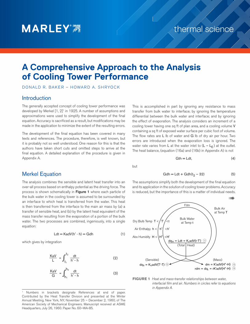
Merkel EquationThe analysis combines the sensible and latent heat transfer into an over-all process based on enthalpy potential as the driving force. The process is shown schematically in Figure 1 where each particle of the bulk water in the cooling tower is assumed to be surrounded by an interface to which heat is transferred from the water. This heat is then transferred from the interface to the main air mass by (a) a transfer of sensible heat, and (b) by the latent heat equivalent of the mass transfer resulting from the evaporation of a portion of the bulk water. The two processes are combined, ingeniously, into a single equation:
Ldt = KadV(h' - h) = Gdh (1)
which gives by integration
This is accomplished in part by ignoring any resistance to mass transfer from bulk water to interface; by ignoring the temperature differential between the bulk water and interface; and by ignoring the effect of evaporation. The analysis considers an increment of a cooling tower having one sq ft of plan area, and a cooling volume V containing a sq ft of exposed water surface per cubic foot of volume. The flow rates are L lb of water and G Ib of dry air per hour. Two errors are introduced when the evaporation loss is ignored. The water rate varies from L at the water inlet to (L – LE ) at the outlet. The heat balance, (equation (16a) and (16b) in Appendix A) is not
Gth = Ldt, (4)
but
Gdh = Ldt + Gdh(t2 – 32) (5)
The assumptions simplify both the development of the final equation and its application in the solution of cooling tower problems. Accuracy is reduced, but the importance of this is a matter of individual needs.
1 Numbers in brackets designate References at end of paper. Contributed by the Heat Transfer Division and presented at the Winter Annual Meeting, New York, NY, November 25 – December 2, 1960, of The American Society of Mechanical Engineers. Manuscript received at ASME Headquarters, July 26, 1960. Paper No. 60–WA-85.
KaVL ∫= dt
h' - h
t2
t1
(2)
KaVG ∫= dt
h' - h
h2
h1
(3)
Film
(Total Heat)
(Sensible) (Mass)
Dry Bulb Temp T < T' <t
Air Enthalpy h < h" <h'
Abs Humidity H < H" <H'
Bulk Waterat Temp t
Bulk Airat Temp T
dqW = Ldt = KLadV(t-T')
rdm = dqL = rK'adV(H"-H)dm = K'adV(H"-H)dqS = KGadV(T'-T)
11
12 13
14
FIGURE 1 Heat and mass-transfer relationships between water, interfacial film and air. Numbers in circles refer to equations in Appendix A.
➠
Application of Basic EquationEquation (2) or (3), conforms to the transfer-unit concept in which a transfer-unit represents the size or extent of the equipment that allows the transfer to come to equilibrium. The integrated value corresponding to a given set of conditions is called the Number of Transfer Units (NTH), which is a measure of the degree-of-difficulty of the problem.
The equation is not self-sufficient so does not lend itself to direct mathematical solution. The usual procedure is to integrate it in connection with the heat balance expressed by equation (4). The basic equation reflects mass and energy balances at any point within a cooling tower, but without regard to the relative motion of the two streams. It is solved by some means of mechanical integration that considers the relative motion involved in counterflow or crossflow cooling, as the case may be.
The counterflow-cooling diagram is represented graphically in Figure 2. Water entering the top of the cooling tower at t, is surrounded by an interfacial film that is assumed to be saturated with water vapor at the bulk water temperature This corresponds to point A on the saturation curve. As the water is cooled to t2, the film enthalpy follows the saturation curve to point B. Air entering the base of the cooling tower at wet-bulb temperature TWB has an enthalpy corresponding to C' on the saturation curve The driving force at the base of the cooling tower is represented by the vertical distance BC. Heat removed from the water is added to the air so its enthalpy increases along the straight line CD, having a slope equaling the L/G ratio and terminating at a point vertically below point A. The counterflow integration is explained in detail in Appendix B.
Air and water conditions are constant across any horizontal section of a counterflow cooling tower. Both conditions vary horizontally and vertically in a crossflow cooling tower as shown in Figure 3. Hot water enters across the OX axis and is cooled as it falls downward. The solid lines show constant water temperatures. Air entering from the left across the OY axis is heated as it moves to the right, and the dotted lines represent constant enthalpies.
Because of the horizontal and vertical variation, the cross section must be divided into unit-volumes having a width dx and a height dy, so that dV in equation (1) is replaced with dxdy and it becomes
Ldtdx = Gdhdy = Kadxdy(h' -h) (6)
Cross-sectional shape is taken into account by considering dx/dy = w/z so that dL/dG = L/G. The ratio of the overall flow rates thus apply to the incremental volumes and the integration considers an equal number of horizontal and vertical increments.
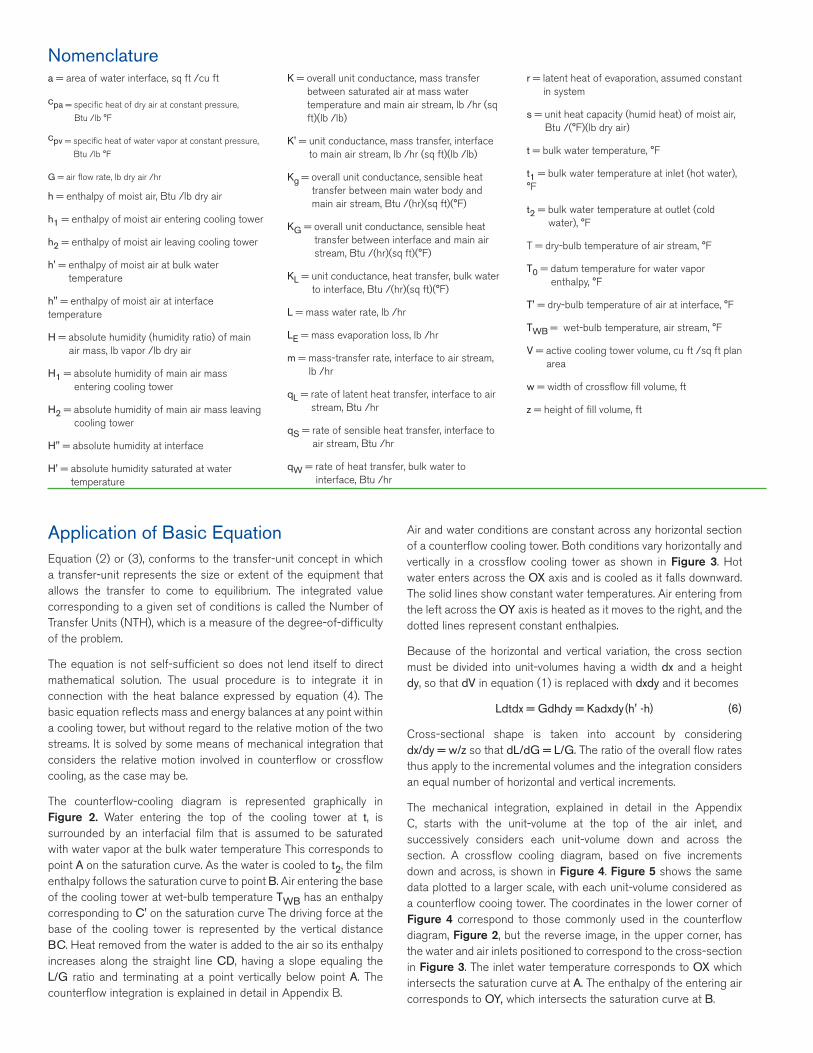
The mechanical integration, explained in detail in the Appendix C, starts with the unit-volume at the top of the air inlet, and successively considers each unit-volume down and across the section. A crossflow cooling diagram, based on five increments down and across, is shown in Figure 4. Figure 5 shows the same data plotted to a larger scale, with each unit-volume considered as a counterflow cooing tower. The coordinates in the lower corner of Figure 4 correspond to those commonly used in the counterflow diagram, Figure 2, but the reverse image, in the upper corner, has the water and air inlets positioned to correspond to the cross-section in Figure 3. The inlet water temperature corresponds to OX which intersects the saturation curve at A. The enthalpy of the entering air corresponds to OY, which intersects the saturation curve at B.
a = area of water interface, sq ft /cu ft
cpa = specific heat of dry air at constant pressure,
Btu /lb °F
cpv = specific heat of water vapor at constant pressure,
Btu /lb °F
G = air flow rate, lb dry air /hr
h = enthalpy of moist air, Btu /lb dry air
h1 = enthalpy of moist air entering cooling tower
h2 = enthalpy of moist air leaving cooling tower
h' = enthalpy of moist air at bulk water temperature
h" = enthalpy of moist air at interface temperature
H = absolute humidity (humidity ratio) of main air mass, lb vapor /lb dry air
H1 = absolute humidity of main air mass entering cooling tower
H2 = absolute humidity of main air mass leaving cooling tower
H" = absolute humidity at interface
H' = absolute humidity saturated at water temperature
K = overall unit conductance, mass transfer between saturated air at mass water temperature and main air stream, lb /hr (sq ft)(lb /lb)
K' = unit conductance, mass transfer, interface to main air stream, lb /hr (sq ft)(lb /lb)
Kg = overall unit conductance, sensible heat transfer between main water body and main air stream, Btu /(hr)(sq ft)(°F)
KG = overall unit conductance, sensible heat transfer between interface and main air stream, Btu /(hr)(sq ft)(°F)
KL = unit conductance, heat transfer, bulk water to interface, Btu /(hr)(sq ft)(°F)
L = mass water rate, lb /hr
LE = mass evaporation loss, lb /hr
m = mass-transfer rate, interface to air stream, lb /hr
qL = rate of latent heat transfer, interface to air stream, Btu /hr
qS = rate of sensible heat transfer, interface to air stream, Btu /hr
qW = rate of heat transfer, bulk water to interface, Btu /hr
r = latent heat of evaporation, assumed constant in system
s = unit heat capacity (humid heat) of moist air, Btu /(°F)(lb dry air)
t = bulk water temperature, °F
t1 = bulk water temperature at inlet (hot water), °F
t2 = bulk water temperature at outlet (cold water), °F
T = dry-bulb temperature of air stream, °F
T0 = datum temperature for water vapor enthalpy, °F
T' = dry-bulb temperature of air at interface, °F
TWB = wet-bulb temperature, air stream, °F
V = active cooling tower volume, cu ft /sq ft plan area
w = width of crossflow fill volume, ft
z = height of fill volume, ft
Nomenclature

Logical reasoning will show that water falling through any vertical section will always be moving toward colder air. For a cooling tower of infinite height, the water will be approaching air at the entering wet-bulb temperature as a limit. The water temperature, therefore, approaches B as a limit at infinite height, and follows one of the curves of the family radiating from B. The family of curves has OY as one limit at the air inlet and the saturation curve AB as the other limit for a vertical section at infinite width.
Air moving through any horizontal section is always moving toward hotter water. For a cooling tower of infinite width, air will be approaching water at the hot-water temperature as a limit. The air moving through any horizontal section, therefore, approaches A as a limit, following one of the curves of the family radiating from A. This family of curves varies from OX as one limit at the water inlet to AB for a cooling tower of infinite height.
The counterflow cooling tower diagram considers the area between the saturation curve and the air-operating line CD in Figure 2. The crossflow diagram considers the saturation curve and the area of overlap of the two families of curves radiating from A and B.
Cooling Tower CoefficientsThe theoretical calculations reduce a set of performance conditions to a numerical value that serves as a measure of the degree-of-difficulty. The NTU corresponding to a set of hypothetical conditions is called the required coefficient and is an evaluation of the problem. The same calculations applied to a set of test conditions is called the available coefficient of the cooling tower involved.
Required Coefficient. Cooling towers are specified in terms of hot water, cold water, and wet-bulb temperature and the water rate that will be cooled at these temperatures. The same temperature conditions are considered as variables in the basic equations, but the remaining variable is L/G ratio instead of water rate. The L/G ratio is convertible into water rate when the air rate is known. ➠
FIGURE 2 Counterflow cooling diagram
FIGURE 3 Water temperature and air enthalpy variation through a crossflow cooling tower
FIGURE 4 Crossflow cooling diagram
60 80
Temperature °F
Ent
halp
y, B
tu p
er lb
dry
air
100 120
140
A
D
h1
t1t2
h2
TWB
h
B
CC'
L /G
120
100
80
60
40
20
O
Z
Y
W XWater Inlet
Air h
Water L
Air
Inle
t
40 41 42 43 44
30 31 32 33 34
20 21 22 23 24
10 11 12 13 14
00 01 02 03 04 0n
n0 n1 n2 n3 n4 nn
1n
2n
3n
4n
70
70
80
90
100
110
120
80
30 40 50 60 70 80 90 100 110 120
120
110
100
90
80
70
60
50
40
3090 100 110 120
Temperature °F
Tem
pera
ture
°F
Enthalpy, Btu per lb dry air
Ent
halp
y, B
tu p
er lb
dry
air
A
A
B
B
Y
Y
X
XO
O
A given set of temperature conditions may be achieved by a wide range of L/G ratios. This is shown diagrammatically for the counterflow cooling tower in Figure 6. The imaginary situation corresponding to an infinite air rate results in L/G = 0 which is represented by the horizontal operating line CD0. This results in the maximum driving force and the minimum required coefficient. As the air rate decreases progressively, the L/G ratio increases and the slope of the operating line increases. This decreases the driving
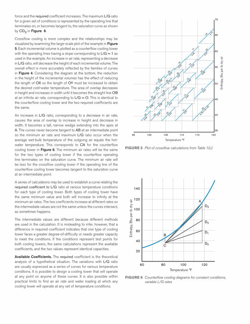
force and the required coefficient increases. The maximum L/G ratio for a given set of conditions is represented by the operating line that terminates on, or becomes tangent to, the saturation curve as shown by CD3 in Figure 6.
Crossflow cooling is more complex and the relationships may be visualized by examining the large-scale plot of the example in Figure 5. Each incremental volume is plotted as a counterflow cooling tower with the operating lines having a slope corresponding to L/G = 1 as used in the example. An increase in air rate, representing a decrease in L/G ratio, will decrease the height of each incremental volume. The overall effect is more accurately reflected by the families of curves in Figure 4. Considering the diagram at the bottom, the reduction in the height of the incremental volumes has the effect of reducing the length of OX so the length of OY must be increased to obtain the desired cold-water temperature. The area of overlap decreases in height and increases in width until it becomes the straight line OB at an infinite air rate, corresponding to L/G = O. This is identical to the counterflow cooling tower and the two required coefficients are the same.
An increase in L/G ratio, corresponding to a decrease in air rate, causes the area of overlap to increase in height and decrease in width. It becomes a tall, narrow wedge extending into the apex at A. The curves never become tangent to AB at an intermediate point so the minimum air rate and maximum L/G ratio occur when the average wet-bulb temperature of the outgoing air equals the hot-water temperature. This corresponds to CA for the counterflow cooling tower in Figure 6. The minimum air rates will be the same for the two types of cooling tower if the counterflow operating line terminates on the saturation curve. The minimum air rate will be less for the crossflow cooling tower if the operating line of the counterflow cooling tower becomes tangent to the saturation curve at an intermediate point.
A series of calculations may be used to establish a curve relating the required coefficient to L/G ratio at various temperature conditions for each type of cooling tower. Both types of cooling tower have the same minimum value and both will increase to infinity at the minimum air rates. The two coefficients increase at different rates so the intermediate values are not the same unless the curves intersect, as sometimes happens.
The intermediate values are different because different methods are used in the calculation. It is misleading to infer, however, that a difference in required coefficient indicates that one type of cooling tower faces a greater degree-of-difficulty or needs greater capacity to meet the conditions. If the conditions represent test points for both cooling towers, the same calculations represent the available coefficients, and the two values represent identical capacities.
Available Coefficients. The required coefficient is the theoretical analysis of a hypothetical situation. The variations with L/G ratio are usually expressed as a series of curves for various temperature conditions. It is possible to design a cooling tower that will operate at any point on anyone of these curves. It is also possible within practical limits to find an air rate and water loading at which any cooling tower will operate at any set of temperature conditions.
35
40
45
50
55
60
65
95 100 105 110 115 120
70
14
24
3433
32
31
30
44
43
42
4140
13
12
1110
25
22
2120
0403
0201
00
4.77
4.05
4.33
4.62
4.94
5.27
3.50
3.67
3.65
4.04
4.24
3.15
3.27
3.38
3.50
3.04
2.68
2.14
2.80
2.88
2.94
5.21
5.69
6.22
6.79
= ∆t x
∆h
Ent
halp
y, B
tu p
er lb
dry
air
Temperature °F
FIGURE 5 Plot of crossflow calculations from Table 1(c)
FIGURE 6 Counterflow cooling diagrams for constant conditions, variable L/G rates
60 80
Temperature °F
Ent
halp
y, B
tu p
er lb
dry
air
100 120
140
120
100
80
60
40
20
AD3
D2
D1
D0
B
C
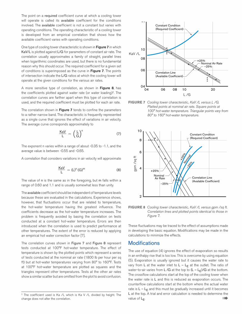
FIGURE 7 Cooling tower characteristic, KaV /L versus L /G. Platted points at nominal air rate. Square points at 100° hot-water temperature. Triangular points vary from 80° to 160° hot-water temperature.
FIGURE 8 Cooling tower characteristic, KaV /L versus gpm /sq ft. Correlation lines and plotted points identical to those in Figure 7.
The point on a required coefficient curve at which a cooling tower will operate is called its available coefficient for the conditions involved. The available coefficient is not a constant but varies with operating conditions. The operating characteristic of a cooling tower is developed from an empirical correlation that shows how the available coefficient varies with operating conditions.
One type of cooling tower characteristic is shown in Figure 7 in which KaV/L is plotted against L/G for parameters of constant air rate. The correlation usually approximates a family of straight, parallel lines when logarithmic coordinates are used, but there is no fundamental reason why this should occur. The required coefficient for a given set of conditions is superimposed as the curve in Figure 7. The points of intersection indicate the L/G ratios at which the cooling tower will operate at the given conditions for the various air rates.
A more sensitive type of correlation, as shown in Figure 8, has the coefficients plotted against water rate (or water loading)2. The correlation curves are farther apart when this type of correlation is used, and the required coefficient must be plotted for each air rate.
The correlation shown in Figure 7 tends to confine the parameters to a rather narrow band. The characteristic is frequently represented as a single curve that ignores the effect of variations in air velocity. The average curve corresponds approximately to
The exponent n varies within a range of about -0.35 to -1.1, and the average value is between -0.55 and -0.65.
A correlation that considers variations in air velocity will approximate
The value of n is the same as in the foregoing, but m falls within a range of 0.60 and 1.1 and is usually somewhat less than unity.
The available coefficient should be independent of temperature levels because these are evaluated in the calculations. Experience shows, however, that fluctuations occur that are related to temperature, the hot-water temperature having the greatest influence. The coefficients decrease as the hot-water temperature increases. The problem is frequently avoided by basing the correlation on tests conducted at a constant hot-water temperature. Errors are then introduced when the correlation is used to predict performance at other temperatures. The extent of the error is reduced by applying an empirical hot water correction factor [7].
The correlation curves shown in Figure 7 and Figure 8 represent tests conducted at 100°F hot-water temperature. The effect of temperature is shown by the plotted points which represent a series of tests conducted at the nominal air rate (1800 Ib per hour per sq ft) but at hot-water temperatures varying from 80° to 160°F. Tests at 100°F hot-water temperature are plotted as squares and the triangles represent other temperatures. Tests at the other air rates show a similar scatter but are omitted from the plot to avoid confusion.
2 The coefficient used is Ka /L which is Ka V /L divided by height. The change does not alter the correlation.
KaVL
LG
(7)∼ ( )n
KaVL
(8)∼ (L)n (G)m
0404
06
08
10
20
06 08
Constant Condition(Required Coefficient)
+25%Nominal Air Rate
–25%
Correlation Line(Available Coefficient)
10 20L /G
KaV /L
042
4
6
8
10
06 08 10 20
gpm
/sq
ft
KaV /L
Constant Condition(Required Coefficient)
Correlation Line(Available Coefficient)
+25%
+25%
–25%
Nom
inal
Nominal Air Rate
–25%
These fluctuations may be traced to the effect of assumptions made in developing the basic equation. Modifications may be made in the calculations to minimize the effects.
Modifications The use of equation (4) ignores the effect of evaporation so results in an enthalpy rise that is too low. This is overcome by using equation (5). Evaporation is usually ignored but it causes the water rate to vary from L at the water inlet to L – LE at the outlet. The ratio of water-to-air varies from L /G at the top to (L – LE)/G at the bottom. The crossflow calculations start at the top of the cooling tower when the water rate is L and this is reduced as evaporation occurs. The counterflow calculations start at the bottom where the actual water rate is L – LE and this must be gradually increased until it becomes L at the top. A trial and error calculation is needed to determine the value of LE. ➠
Heat Balance Corrections. The effect of these two corrections is shown in Table 1 for counterflow calculations. Example I relates NTU to range when calculated in the usual manner without modification. Example II shows the effect of calculating the enthalpy rise with equation (5), but considers a constant L /G ratio. Example III uses equation (5) and also varies the water rate so that (L – LE)/G = 1.1633 at the bottom and this gradually increases to the design condition of L /G = 1.20 at the water inlet.
The use of equation (5) in Example II results in a 4.4% increase in NTU at a 4O° range. Example III is more accurate because it also varies the water rate, and this increases the NTU by only 1.34% at the 40° range. These changes tend to counteract the effect of temperature level on the coefficients.
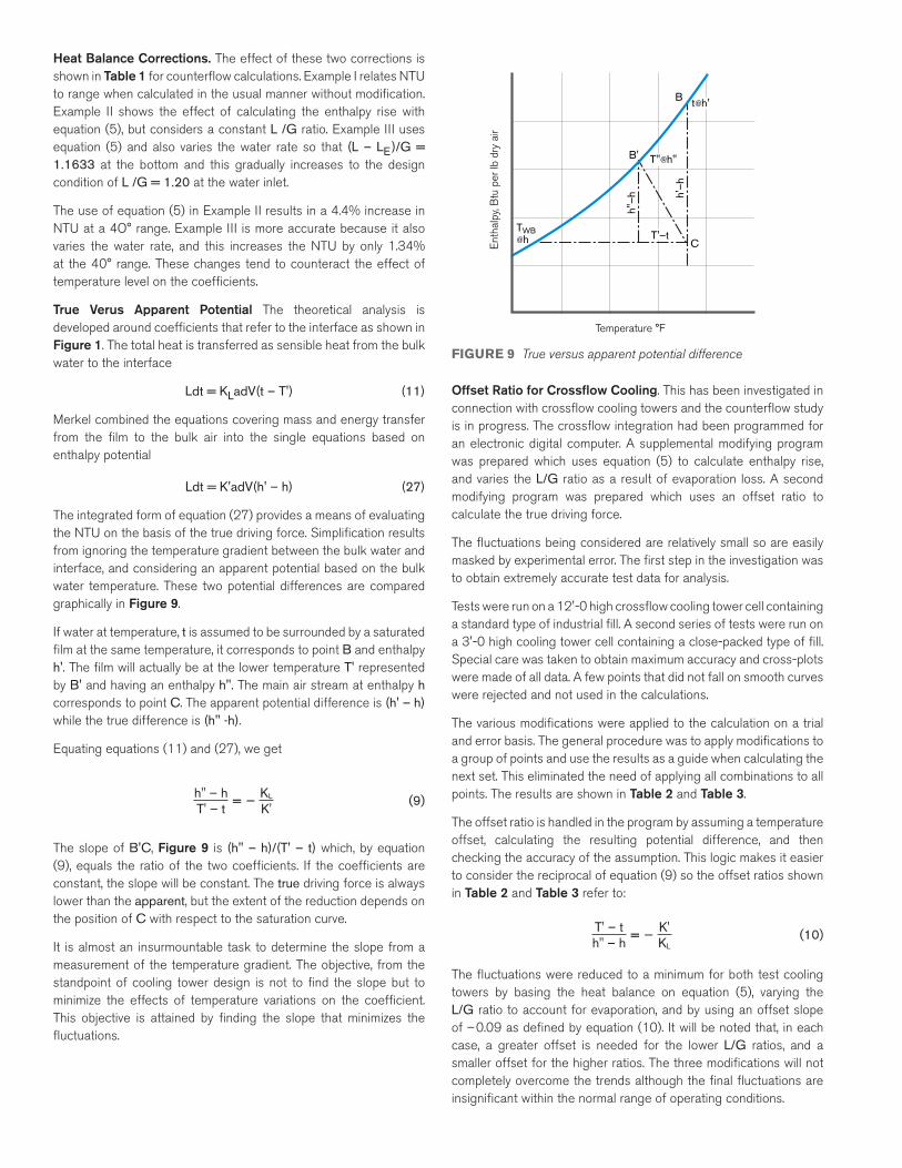
True Verus Apparent Potential The theoretical analysis is developed around coefficients that refer to the interface as shown in Figure 1. The total heat is transferred as sensible heat from the bulk water to the interface
Ldt = KLadV(t – T') (11)
Merkel combined the equations covering mass and energy transfer from the film to the bulk air into the single equations based on enthalpy potential
Ldt = K'adV(h' – h) (27)
The integrated form of equation (27) provides a means of evaluating the NTU on the basis of the true driving force. Simplification results from ignoring the temperature gradient between the bulk water and interface, and considering an apparent potential based on the bulk water temperature. These two potential differences are compared graphically in Figure 9.
If water at temperature, t is assumed to be surrounded by a saturated film at the same temperature, it corresponds to point B and enthalpy h'. The film will actually be at the lower temperature T' represented by B' and having an enthalpy h". The main air stream at enthalpy h corresponds to point C. The apparent potential difference is (h' – h) while the true difference is (h" -h).
Equating equations (11) and (27), we get
The slope of B'C, Figure 9 is (h" – h)/(T' – t) which, by equation (9), equals the ratio of the two coefficients. If the coefficients are constant, the slope will be constant. The true driving force is always lower than the apparent, but the extent of the reduction depends on the position of C with respect to the saturation curve.
It is almost an insurmountable task to determine the slope from a measurement of the temperature gradient. The objective, from the standpoint of cooling tower design is not to find the slope but to minimize the effects of temperature variations on the coefficient. This objective is attained by finding the slope that minimizes the fluctuations.
h" – hT' – t
KL
K'(9)= –
Ent
halp
y, B
tu p
er lb
dry
air
Temperature °F
B'
B
C
t@h'
T"@h"
@h T'–t
h'–h
h"–h
TWB
FIGURE 9 True versus apparent potential difference
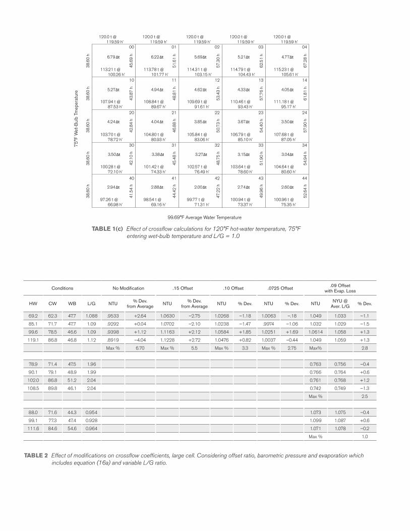
Offset Ratio for Crossflow Cooling. This has been investigated in connection with crossflow cooling towers and the counterflow study is in progress. The crossflow integration had been programmed for an electronic digital computer. A supplemental modifying program was prepared which uses equation (5) to calculate enthalpy rise, and varies the L/G ratio as a result of evaporation loss. A second modifying program was prepared which uses an offset ratio to calculate the true driving force.
The fluctuations being considered are relatively small so are easily masked by experimental error. The first step in the investigation was to obtain extremely accurate test data for analysis.
Tests were run on a 12'-0 high crossflow cooling tower cell containing a standard type of industrial fill. A second series of tests were run on a 3'-0 high cooling tower cell containing a close-packed type of fill. Special care was taken to obtain maximum accuracy and cross-plots were made of all data. A few points that did not fall on smooth curves were rejected and not used in the calculations.
The various modifications were applied to the calculation on a trial and error basis. The general procedure was to apply modifications to a group of points and use the results as a guide when calculating the next set. This eliminated the need of applying all combinations to all points. The results are shown in Table 2 and Table 3.
The offset ratio is handled in the program by assuming a temperature offset, calculating the resulting potential difference, and then checking the accuracy of the assumption. This logic makes it easier to consider the reciprocal of equation (9) so the offset ratios shown in Table 2 and Table 3 refer to:
The fluctuations were reduced to a minimum for both test cooling towers by basing the heat balance on equation (5), varying the L/G ratio to account for evaporation, and by using an offset slope of –0.09 as defined by equation (10). It will be noted that, in each case, a greater offset is needed for the lower L/G ratios, and a smaller offset for the higher ratios. The three modifications will not completely overcome the trends although the final fluctuations are insignificant within the normal range of operating conditions.
T' – th" – h
K'KL
(10)= –

RangeExample I
No Modification NTU
Example II Equation (16a), Constant L/G
NTU
Example II Equation (16a), Variable L/G
NTU L/G
1 0.1048 0.1051 0.1046 1.1633
2 0.2106 0.2115 0.2105 1.1641
3 0.3171 0.3192 0.3170 1.1649
4 0.4246 0.4279 0.4245 1.1658
5 0.5317 0.5372 0.5317 1.1666
10 1.0531 1.0762 1.0564 1.1710
15 1.5294 1.5770 1.5387 1.1759
20 1.9350 2.0080 1.9523 1.1802
25 2.2631 2.9577 2.2886 1.1850
30 2.5203 2.6315 2.5533 1.1899
35 2.7244 2.8422 2.7581 1.1949
40 2.8775 3.0037 2.9159 1.2000
TABLE 1(a) Effect of modifications on counterflow coefficients. Using equation (16a) for heat balance and varying L/G ration
TABLE 1(b) Example of counterflow calculation of NTU for 80°F cold-water temperature, 70°F entering wet-bulb temperature and L/G 1.20.
1 2 3 4 5
Water Temperature
t
Enthalpy at t h'
Enthalpy of air
h
Enthalphy difference
(h' – h)
I
(h' – h)
80 43.69 34.09 9.60 .1043
81 44.78 35.29 9.49 .1055
82 45.90 36.49 9.41 .1067
83 47.04 37.69 9.35 .1070
84 48.20 38.83 9.33 .1072
85 49.43 40.09 9.34 .1071
90 55.93 46.09 9.84 .1016
95 63.32 52.09 10.23 .0977
100 71.73 58.09 13.64 .0734
105 81.34 64.09 17.25 .0580
6 7 8 9
I
(h' – h)
dt
(h' – h)
dt
(h' – h)
Range °F
.1049 .1049 .1049 1
.1059 .1059 .2108 2
.1067 .1067 .3175 3
.1071 .1071 .4246 4
.1072 .1072 .5318 5
.1043 .5215 1.0533 10
.0996 .4980 1.5513 15
.0856 .4280 1.9793 20
.0657 .3285 2.3078 25
∫mean
The first calculations were based on the properties of air at the standard barometric pressure of 29.92" Hg which is common practice. The tests were conducted at a slightly lower atmospheric pressure· so the psychrometric subroutines were altered to reflect conditions at the existing pressure. The last two columns in Table 3 show that nothing was gained by this change.
Conclusions The difficulties encountered in predicting cooling tower performance are directly related to the precision that is required. There is no general agreement on what constitutes an acceptable degree of accuracy. The users are reluctant to allow a tolerance of 1⁄2° in approach when acceptance tests are involved. Cooling tower capacity is more accurately expressed in terms of water rate for a given set of conditions. This capacity is approximately proportional to variations in approach when other conditions are constant, so 1⁄2° corresponds to a difference of 10 per cent in capacity for a 5° approach. This provides an indication of what constitutes a reasonable maximum limit of acceptable tolerance.
The existence of the need for a means of predicting performance may be taken as an indication that the usual procedures are not giving satisfactory results. The problem may be due to inexperience or to inadequate test, procedures that do not provide reliable test results, or to errors introduced by the method of calculation. All of these items are involved and an improvement in one will provide a means of improving the others.
The needs of the user and manufacturer are not the same, and the difficulties encountered will vary with the type of problem involved. These include comparing test results to guarantee, using test results to predict performance at other conditions, comparing capacities when bids are analyzed and developing the rating table for a new cooling tower.
This paper deals with the errors in the mathematical analysis and describes the means of minimizing them. Each improvement makes the analysis more difficult. No attempt has been made to evaluate this or to consider the effect of each source of error on the overall accuracy.
➠
Conditions No Modification .15 Offset .10 Offset .0725 Offset .09 Offset with Evap. Loss
HW CW WB L/G NTU % Dev. from Average NTU % Dev.
from Average NTU % Dev. NTU % Dev. NTU NYU @ Aver. L/G % Dev.
69.2 62.3 47.7 1.088 .9533 +2.64 1.0630 –2.75 1.0268 –1.18 1.0063 –.18 1.049 1.033 –1.1
85.1 71.7 47.7 1.09 .9292 +0.04 1.0702 –2.10 1.0238 –1.47 .9974 –1.06 1.032 1.029 –1.5
99.6 78.5 46.6 1.09 .9398 +1.12 1.1163 +2.12 1.0584 +1.85 1.0251 +1.69 1.0614 1.058 +1.3
119.1 86.8 46.8 1.12 .8919 –4.04 1.1228 +2.72 1.0476 +0.82 1.0037 –0.44 1.049 1.059 +1.3
Max % 6.70 Max % 5.5 Max % 3.3 Max % 2.75 Max% 2.8
78.9 71.4 47.5 1.96 0.763 0.756 –0.4
90.1 79.1 48.9 1.99 0.766 0.764 +0.6
102.0 86.8 51.2 2.04 0.761 0.768 +1.2
108.5 89.8 46.1 2.04 0.742 0.749 –1.3
Max % 2.5
88.0 71.6 44.3 0.954 1.073 1.075 –0.4
99.1 77.3 47.4 0.928 1.099 1.087 +0.6
111.6 84.6 54.6 0.964 1.071 1.078 –0.2
Max % 1.0
120.0 t @ 119.59 h’
120.0 t @ 119.59 h’
120.0 t @ 119.59 h’
120.0 t @ 119.59 h’
120.0 t @ 119.59 h’
113.21 t @ 100.26 h’
113.78 t @ 101.77 h’
114.31 t @ 103.15 h’
114.79 t @ 104.43 h’
115.23 t @ 105.61 h’
107.94 t @ 87.53 h’
108.84 t @ 89.67 h’
109.69 t @ 91.61 h’
110.46 t @ 93.43 h’
111.18 t @ 95.17 h’
103.70 t @ 78.72 h’
104.80 t @ 80.93 h’
105.84 t @ 83.06 h’
106.79 t @ 85.10 h’
107.68 t @ 87.05 h’
100.28 t @ 72.10 h’
101.42 t @ 74.33 h’
102.57 t @ 76.49 h’
103.64 t @ 78.60 h’
104.64 t @ 80.60 h’
97.26 t @ 66.98 h’
98.54 t @ 69.16 h’
99.77 t @ 71.31 h’
100.94 t @ 73.37 h’
100.96 t @ 75.35 h’
6.79∆t 6.22∆t 5.69∆t 5.21∆t 4.77∆t
5.27∆t 4.94∆t 4.62∆t 4.33∆t 4.05∆t
4.24∆t 4.04∆t 3.85∆t 3.67∆t 3.50∆t
3.50∆t 3.38∆t 3.27∆t 3.15∆t 3.04∆t
2.94∆t 2.88∆t 2.00∆t 2.74∆t 2.60∆t
38
.60
h
45
.69
h
51
.61
h
57
.30
h
62
.51
h
67
.28
h
38
.60
h
43
.87
h
48
.81
h
53
.43
h
57
.76
h
61
.81
h
38
.60
h
42
.84
h
46
.88
h
50
.73
h
54
.40
h
57
.90
h
38
.60
h
42
.10
h
45
.48
h
48
.75
h
51
.90
h
54
.94
h
38
.60
h
41
.54
h
44
.42
h
47
.22
h
49
.96
h
52
.64
h
00 01 02 03 04
10 11 12 13 14
20 21 22 23 24
30 31 32 33 34
40 41 42 43 44
75
°F W
et-B
ulb
Tmep
erat
ure
99.69°F Average Water Temperature
TABLE 1(c) Effect of crossflow calculations for 120°F hot-water temperature, 75°F entering wet-bulb temperature and L/G = 1.0
TABLE 2 Effect of modifications on crossflow coefficients, large cell. Considering offset ratio, barometric pressure and evaporation which includes equation (16a) and variable L/G ratio.

Conditions .07 Offset .07 Offset with Evap.
.15 Offset with Evap.
.10 Offset with Evap.
.09 Offset with Evap.
.09 Offset with Evap.
@ 29.14" Hg
HW CW WB L/G NTU % Dev. NTU % Dev. NTU % Dev. NTU % Dev. NTU % Dev. NTU % Dev.
70.4 66.9 55.2 1.74 .6053 +3.10 .6143 +2.64 .6533 –4.14 .6293 +.016 .6243 +.99 .6241 +.68
100.7 87.5 55.7 1.70 .5851 –.34
119.5 97.8 96.0 1.765 .6258 –.54 .6146
150.3 111.1 62.1 1.76 .5709 –2.76 .5826 –2.64 .7097 +4.41 .6326 +.54 .6157 –.41 .6156 –.68
Max % 5.86 5.28 8.28 1.08 1.57 1.36
79.7 69.8 57.2 .654 1.0697 +.86 1.1062 –.87 1.0968 –.24 1.0965 –.35
120.4 86.1 58.1 .656 1.1138 –.20 1.0908 –.21
150.5 93.1 58.9 .659 1.0515 –.86 1.1279 +1.07 1.1044 +.45 1.142 +.35
Max % 1.72 1.94 .69 .70
We are faced with the unfortunate fact that it is difficult to attain an accuracy that is within our maximum limits of acceptability although this does not represent a high degree of precision. Care is needed to obtain test data having an accuracy of 1⁄2° or 10% in capacity. The method of analysis may have inherent errors that exceed these limits. The general failure to obtain satisfactory results may be due, to a large extent, to the failure to exert sufficient effort to solve a problem that is inherently difficult. It may be that a justifiable effort will not yield an answer of acceptable accuracy.
The object of this paper is to describe methods that will give a satisfactory answer, without regard to the effort needed. A method that does not provide an acceptable degree of accuracy is all but worthless, regardless of how easy it may be. The limits of acceptability and the effort to be expended will be up to the individual, and each will obviously seek the easiest means of attaining the desired end.
APPENDIX A
Development of Basic EquationsHeat is removed from the water by a transfer of sensible heat due to a difference in temperature levels, and by the latent heat equivalent of the mass transfer resulting from the evaporation of a portion of the circulating water. Merkel combined these into a single process based on enthalpy potential differences as the driving force.
The analysis [3] considers an increment of a cooling tower having one sq ft of plan area, and a cooling volume V, containing a sq ft of exposed water surface per cubic foot of volume. Flowing through the cooling tower are L Ib of water and G lb of dry air per hour.
Transfer Rate Equations. The air at any point has a dry bulb temperature T, an absolute humidity (lb water vapor per lb dry air) H, and a corresponding enthalpy h. The water, having a bulk temperature t, Figure 1 is surrounded by an interfacial film having a temperature T'. The temperature gradients are such that T < T' < t.
The specific heat of water is assumed to be unity and a constant, so the symbol will be omitted from the equations for simplicity. The rate of heat transfer from the bulk water to the interface is:
dqW = Ldt = KLasV(t – T') (11)
TABLE 3 Effect of modifications on crossflow coefficients, small cell. Considering offset ratio, barometric pressure and evaporation which includes equation (16a) and variable L/G ratio.
A portion of this heat is transferred as sensible heat from the interface of the main air stream. This rate is:
dqS = KGadV(T' – T) (12)
The interfacial air film is assumed to be saturated with water vapor at temperature T', having a corresponding absolute humidity H". The procedure is to ignore any resistance to mass transfer from the water to the interface, but to consider the mass transfer of vapor from the film to the air, as
dm = K'adV(H' – H) (13)
Considering the latent heat of evaporation as a constant, r, the mass rate in equation (13) is converted to heat rate by multiplying by r
rdm = dqS = rK'adV(H' – H) (14)
Mass and Energy Balances. Under steady state, the rate of mass leaving the water by evaporation equals the rate of humidity increase of the air, so
dm = GdH (15)
The heat lost by the water equals the heat gained by the air. The usual practice is to ignore the slight reduction in L due to evaporation, in which case
GdH = Ldt (16a)3
3 A more rigorous analysis considers evaporation loss, so L Ib enters but (L – LE) Ib of water leaves the cooling tower, and the heat balance is
G(h2 -h1) = L(t1 – 32) – (L – LE)(t2 – 32) (a)
G(h2 – h1) = L(t1 – t2) + LE(t2 – 32) (b)
since
LE = G(H2 – H1)
G(h2 – h1) = L(t1 – t2) + G(H2 – H1) (t2 – 32) (c)
Expressed as a differential equation,
Gdh = Ldt + GdH(t2 – 32) (16b)
The last term in equation (16b) represents the heat required to raise the liquid water evaporated from the base (32°F) to the cold-water temperature. An enthalpy rise calculated by equation (16a) is low by an amount corresponding to this heat of the liquid.
➠
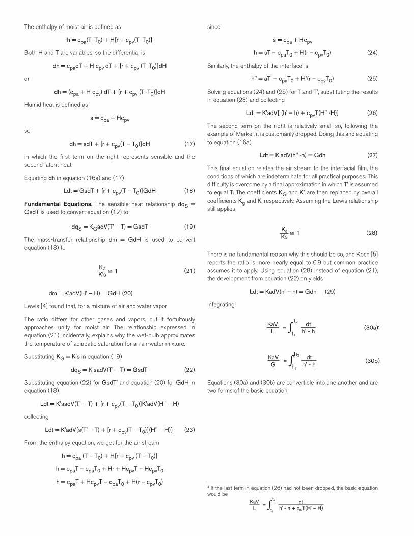
The enthalpy of moist air is defined as
h = cpa(T -T0) + H[r + cpv(T -T0)]
Both H and T are variables, so the differential is
dh = cpadT + H cpv dT + [r + cpv (T -T0)]dH
or
dh = (cpa + H cpv) dT + [r + cpv (T -T0)]dH
Humid heat is defined as
s = cpa + Hcpv
so
dh = sdT + [r + cpv(T – T0)]dH (17)
in which the first term on the right represents sensible and the second latent heat.
Equating dh in equation (16a) and (17)
Ldt = GsdT + [r + cpv(T – T0)]GdH (18)
Fundamental Equations. The sensible heat relationship dqS = GsdT is used to convert equation (12) to
dqS = KGadV(T' – T) = GsdT (19)
The mass-transfer relationship dm = GdH is used to convert equation (13) to
dm = K'adV(H' – H) = GdH (20)
Lewis [4] found that, for a mixture of air and water vapor
The ratio differs for other gases and vapors, but it fortuitously approaches unity for moist air. The relationship expressed in equation (21) incidentally, explains why the wet-bulb approximates the temperature of adiabatic saturation for an air-water mixture.
Substituting KG = K's in equation (19)
dqS = K'sadV(T' – T) = GsdT (22)
Substituting equation (22) for GsdT' and equation (20) for GdH in equation (18)
Ldt = K'sadV(T' – T) + [r + cpv(T – T0)]K'adV(H" – H)
collecting
Ldt = K'adV{s(T' – T) + [r + cpv(T – T0)](H" – H)} (23)
From the enthalpy equation, we get for the air stream
h = cpa (T – T0) + H[r + cpv (T – T0)]
h = cpaT – cpaT0 + Hr + HcpvT – HcpvT0
h = cpaT + HcpvT – cpaT0 + H(r – cpvT0)
KG
K's(21) ≅ 1
since
s = cpa + Hcpv
h = sT – cpaT0 + H(r – cpvT0) (24)
Similarly, the enthalpy of the interface is
h" = aT' – cpaT0 + H'(r – cpvT0) (25)
Solving equations (24) and (25) for T and T', substituting the results in equation (23) and collecting
Ldt = K'adV[ (h' – h) + cpvT(H" -H)] (26)
The second term on the right is relatively small so, following the example of Merkel, it is customarily dropped. Doing this and equating to equation (16a)
Ldt = K'adV(h" -h) = Gdh (27)
This final equation relates the air stream to the interfacial film, the conditions of which are indeterminate for all practical purposes. This difficulty is overcome by a final approximation in which T' is assumed to equal T. The coefficients KG and K' are then replaced by overall coefficients Kg and K, respectively. Assuming the Lewis relationship still applies
There is no fundamental reason why this should be so, and Koch [5] reports the ratio is more nearly equal to 0.9 but common practice assumes it to apply. Using equation (28) instead of equation (21), the development from equation (22) on yields
Ldt = KadV(h' – h) = Gdh (29)
Integrating
Equations (30a) and (30b) are convertible into one another and are two forms of the basic equation.
Kg
Ks(28) ≅ 1
KaVL ∫= dt
h' - h
t2
t1
(30a)4
KaVG ∫= dt
h' - h
h2
h1
(30b)
4 If the last term in equation (26) had not been dropped, the basic equation would be
KaVL ∫= dt
h' - h + cpvT(H' – H)
t2
t1
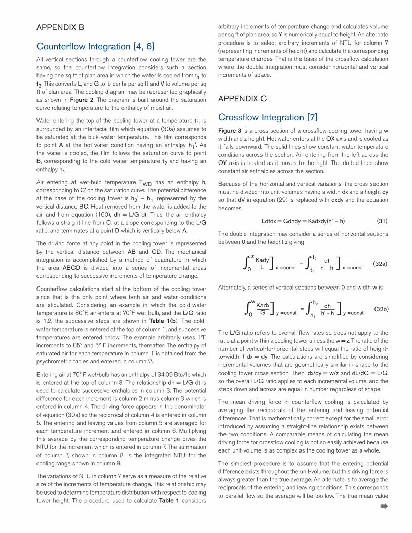
APPENDIX B Counterflow Integration [4, 6] All vertical sections through a counterflow cooling tower are the same, so the counterflow integration considers such a section having one sq ft of plan area in which the water is cooled from t1 to t2. This converts L, and G to lb per hr per sq ft and V to volume per sq ft of plan area. The cooling diagram may be represented graphically as shown in Figure 2. The diagram is built around the saturation curve relating temperature to the enthalpy of moist air.
Water entering the top of the cooling tower at a temperature t1, is surrounded by an interfacial film which equation (30a) assumes to be saturated at the bulk water temperature. This film corresponds to point A at the hot-water condition having an enthalpy h1'. As the water is cooled, the film follows the saturation curve to point B, corresponding to the cold-water temperature t2 and having an enthalpy h1'.
Air entering at wet-bulb temperature TWB has an enthalpy h, corresponding to C' on the saturation curve. The potential difference at the base of the cooling tower is h2' – h1, represented by the vertical distance BC. Heat removed from the water is added to the air, and from equation (160), dh = L/G dt. Thus, the air enthalpy follows a straight line from C, at a slope corresponding to the L/G ratio, and terminates at a point D which is vertically below A.
The driving force at any point in the cooling tower is represented by the vertical distance between AB and CD. The mechanical integration is accomplished by a method of quadrature in which the area ABCD is divided into a series of incremental areas corresponding to successive increments of temperature change.
Counterflow calculations start at the bottom of the cooling tower since that is the only point where both air and water conditions are stipulated. Considering an example in which the cold-water temperature is 80°F, air enters at 70°F wet-bulb, and the L/G ratio is 1.2, the successive steps are shown in Table 1(b). The cold-water temperature is entered at the top of column 1, and successive temperatures are entered below. The example arbitrarily uses 1°F increments to 85° and 5° F increments, thereafter. The enthalpy of saturated air for each temperature in column 1 is obtained from the psychrometric tables and entered in column 2.
Entering air at 70° F wet-bulb has an enthalpy of 34.09 Btu/lb which is entered at the top of column 3. The relationship dh = L/G dt is used to calculate successive enthalpies in column 3. The potential difference for each increment is column 2 minus column 3 which is entered in column 4. The driving force appears in the denominator of equation (30a) so the reciprocal of column 4 is entered in column 5. The entering and leaving values from column 5 are averaged for each temperature increment and entered in column 6. Multiplying this average by the corresponding temperature change gives the NTU for the increment which is entered in column 7. The summation of column 7, shown in column 8, is the integrated NTU for the cooling range shown in column 9.
The variations of NTU in column 7 serve as a measure of the relative size of the increments of temperature change. This relationship may be used to determine temperature distribution with respect to cooling tower height. The procedure used to calculate Table 1 considers
arbitrary increments of temperature change and calculates volume per sq ft of plan area, so Y is numerically equal to height. An alternate procedure is to select arbitrary increments of NTU for column 7 (representing increments of height) and calculate the corresponding temperature changes. That is the basis of the crossflow calculation where the double integration must consider horizontal and vertical increments of space.
APPENDIX C Crossflow Integration [7] Figure 3 is a cross section of a crossflow cooling tower having w width and z height. Hot water enters at the OX axis and is cooled as it falls downward. The solid lines show constant water temperature conditions across the section. Air entering from the left across the OY axis is heated as it moves to the right. The dotted lines show constant air enthalpies across the section.
Because of the horizontal and vertical variations, the cross section must he divided into unit-volumes having a width dx and a height dy so that dV in equation (29) is replaced with dxdy and the equation becomes
Ldtdx = Gdhdy = Kadxdy(h' – h) (31)
The double integration may consider a series of horizontal sections between 0 and the height z giving
Alternately, a series of vertical sections between 0 and width w is
The L/G ratio refers to over-all flow rates so does not apply to the ratio at a point within a cooling tower unless the w = z. The ratio of the number of vertical-to-horizontal steps will equal the ratio of height-to-width if dx = dy. The calculations are simplified by considering incremental volumes that are geometrically similar in shape to the cooling tower cross section. Then, dx/dy = w/z and dL/dG = L/G, so the overall L/G ratio applies to each incremental volume, and the steps down and across are equal in number regardless of shape.
The mean driving force in counterflow cooling is calculated by averaging the reciprocals of the entering and leaving potential differences. That is mathematically correct except for the small error introduced by assuming a straight-line relationship exists between the two conditions. A comparable means of calculating the mean driving force for crossflow cooling is not so easily achieved because each unit-volume is as complex as the cooling tower as a whole.
The simplest procedure is to assume that the entering potential difference exists throughout the unit-volume, but this driving force is always greater than the true average. An alternate is to average the reciprocals of the entering and leaving conditions. This corresponds to parallel flow so the average will be too low. The true mean value
KadyL∫ ∫] ]=
z
x =const x =const0dt
h' - h
t2
t1
(32a)
KadxG∫ ∫] ]=
w
y =const y =const0dh
h' - h
h2
h1
(32b)
➠

is between these two methods. Averaging the potential differences instead of their reciprocals gives a value smaller than the former, but greater than the latter and more closely approximates the true value. That is the recommended method which is used in the following example.
Table 1(c) shows the results of the crossflow calculations when water enters from the top at a uniform temperature of 120°F and air enters from the left at a uniform wet-bulb temperature of 75°F. The over-all L/G ratio is 1.0 and each incremental volume represents 0.1 Transfer-Units.
The crossflow calculations must start at the top of the air inlet since this is the only unit-volume for which both entering air and water conditions are known. The calculations for this first unit-volume are:
1 Inlet conditions Water at 120°F 119.59 h1' Air at 75°F 38.60 h1
80.99 (h1' – h1) in
2 Mean driving force will be less. Assume 67.99 (h' – h)avg corresponding to dt = 6.79°F for 0.1 NTU. Since L/G = 1, dt = dh 3 Outlet conditions
120.0° – 6.79° = 113.21°F 100.26 h2' 38.6 + 6.76 = 45.39 h2
54.87 (h2' – h2) out
4 Checking, 80.99 + 54.87 x 0.1 = 6.79 dt 2
This calculation gives the temperature of the water entering the next lower unit-volume and the enthalpy of the air entering the unit-volume to the right. The calculations proceed down and across as shown in Table 1(c). Averaging 2 steps down and across corresponds to 0.2 NTU, averaging 3 down and across corresponds to 0.3 NTU, and so on.
These relationships are shown in the crossflow diagram in Figure 4, and Figure 5 shows the same data from Table 1(c) plotted to a larger scale. The crossflow diagram is also built around the saturation curve AB and consists of two families of curves representing equations (32a) and (32b). The coordinates in the lower corner of Figure 4 correspond to those used in the counterflow diagram, Figure 2, but the reverse image, in the upper corner, has the water and air inlets positioned to correspond to the cross section in Figure 3. Equation (32a) is the partial integral through successive vertical sections that relates water temperature to height. The inlet water temperature corresponds to OX which intersects the saturation curve at A. The enthalpy of the entering air corresponds to OY which intersects the saturation curve at B.
The water is cooled as it falls through any vertical section, its temperature following one of the family of curves representing equation (32a) that radiate from B. Inspection of the data in Table 1(c) will show the falling water is always moving toward cooler air that approaches the entering wet-bulb temperature as a limit. The curves tend to coincide with OY as one limit at the air inlet and with the saturation curve AB as the other limit for a cooling tower of infinite height.
The air enthalpy increases as it moves across any horizontal section, the enthalpy following one of the family of curves representing equation (32b) that radiate from A. As shown in Table 1(c), the air is always moving toward warmer water that tends to approach the entering water temperature as a limit. These curves tend to coincide with OX as one limit at the water inlet, and with the saturation curve AB as the other limit for a cooling tower of infinite width.
The water in all parts of a cooling tower tends to approach the entering wet-bulb temperature as a limit at point B. The wet-bulb temperature of the air in all parts of the cooling tower tends to approach the hot-water temperature at point A. The single operating line CD of the counterflow diagram in Figure 2 is replaced in the crossflow diagram by a zone represented by the area intersected by the two families of curves.
References 1 F. Merkel, “Verdunstungskuehlung,” VDI Forschungsarbeiten No. 275, Berlin, 1925
2 H. B. Nottage, “Merkel’s Cooling Diagram as a Performance Correlation for Air-Water Evaporative Cooling Systems,” ASHVE Transactions, vol. 47, 1941, p. 429.
3 ASHE Data Book, Basic vol. 6th edition, 1949, p. 361.
4 W. H. Walker, W. K. Lewis, W. H. Adams, and E. R. Gilliland, “Principles of Chemical Engineering,” 3rd edition, McGraw-Hill Book Company, Inc., New York, N. Y., 1937.
5 J. Koch: “Unterschung and Berechnung von Kuehlwerkcn,” VDI Forsehungsheft No. 404, Berlin, 1940.
6 J. Lichtenstein. “Performance and Selection of Mechanical-Draft Cooling Towers,” TRANS. ASME, vol. 65, 1943. p. 779.
7 D. R. Baker and L. T. Mart. “Cooling Tower Characteristics as Determined by the Unit-Volume Coefficient,” Refrigerating Engineering, 1952.
8 H. S. Mickley, “Design of Forced Draft Air Conditioning Equipment.” Chemical Engineering Program, vol. 45. 1949, p. 739.
DISCUSSION
J. Lichtenstein5 This paper reviews the theory and resulting equations currently employed in the calculation and analysis of cooling towers. It points out that the theory neglects certain physical factors, particularly the quantity of water evaporated during the cooling process and the resistance to heat flow from the water to the surrounding saturated air film.
Taking these two factors into account results in equations and methods which become cumbersome and which mask the simple relationships previously established.
It is, of course, legitimate for a theory which attempts to describe a physical phenomena to suppress those factors whose effect on the overall results is small enough as to be within the degree of accuracy of the available testing procedures. Absolute exactitude is sacrificed for the sake of the clarity with which the effects of the essential factors on the phenomena are described.
May I ask the authors, therefore, whether the corrections introduced in their paper would really show up in the results obtained in testing a cooling tower? Their sample calculations do not seem to indicate that if I remember correctly, the best accuracy obtainable between heat balances on the air and water side in the testing of cooling towers is between 5 and 6%.
Since the main effort of the authors is to obtain a “better correlation between theoretical prediction and actual performance of cooling towers, I wonder whether other factors not considered in this paper may not play a more important role. The cooling tower theory, as the authors point out, is based on the performance of a unit cooling tower with air and water quantities well defined. Its application to an actual cooling tower assumes that all unit cooling towers are working alike and in parallel. This of course is not the case. It depends on the design how closely the real cooling tower approaches the idealized cooling tower of equal units. In the actual tower each unit cooling tower works with a different inlet and exit water temperature and with a different (L/G) ratio.
If overall average water inlet and exit temperature obtained in a test are used, then the theory descries the performance of some average unit cooling tower whose location and L/G ratio are unknown.
I wonder whether the introduction of a factor to correct for this situation might not be more effective in aligning theory and practice. In other words, a factor which would measure the degree of approach to the idealized cooling tower on which the theory is based.
The difficulty of obtaining consistent results in the testing of cooling towers is, or course, well known. One of the main factors that governs test results, the atmospheric wet-bulb entering the cooling tower pulsates during the test, is affected by changing wind conditions, and even is affected by the character of the environment in which the cooling tower is installed. A reasonable tolerance in the guarantee for a type of equipment as cooling towers represent, is therefore, unavoidable.
5 Burns & Roe, Inc., New York, NY
R. W. Norris6 The authors are to be congratulated on an excellent technical review of Merkel's original work. Also, they have pointed out where deviations exist from the basic equation which affect cooling tower performance. It is generally agreed that consideration must be given to account for the liquid evaporation loss, as per equation (16b). This becomes more important at the higher L/G ratios whereby the Ib vapor/lb dry air is greatly increased. Also, as noted in the article, increasingly hotter inlet water temperatures result in a lowering of the KaV/L values for a given fill design, once again becoming more pronounced at the higher L/G ratios. These two factors are perhaps the most important deviations from Merkel's equation, especially for a counterflow type cooling tower.
It is hoped that the authors in the future will extend their work into developing and publishing theoretical and actual performance graphs for crossflow cooling towers. Information available on counterflow cooling towers enables the user to more easily evaluate soundness of bids, predict performance at other than design conditions, and compare test results with guarantees. Lichtenstein developed a series of KaV/L versus L/G curves in 1943 for counterflow type cooling towers. More recent work has improved upon these curves, whereby they are sufficiently accurate for setting forth the theoretical requirements to be met by a particular cooling tower design. It is then necessary for the manufacturer to establish experimentally KaV/L versus L/G values for a particular fill spacing, number of grid decks, cooling duty, and so on. Due to the sparse information available it is somewhat difficult for a user to readily approximate cooling tower dimensions and fan horsepower requirements for crossflow towers for a given cooling duty.
Over the past three years we have noted, as an industrial user, a decided and much needed improvement in the number of cooling towers meeting their performance guarantee. At one time, practically every cooling tower we tested failed to meet the guarantee. It is not uncommon now for us to obtain cooling towers producing cold water inlet temperatures slightly exceeding design although we occasionally still find some cooling towers deficient. It appears to us that the methods now available to manufacturers for predicting cooling tower performance are sufficiently accurate from the critical users’ standpoint, and at the same time do not cause a cooling tower manufacturer to bid an oversize cooling tower that penalizes his competitive position. We feel that the next step should be correlation of crossflow data in a form that can readily be used by the industrial cooling tower purchaser.
6 Engineering Department, E. I. du Pont de Nemours & Co., Inc., Wilmington, DE

Authors' Closure We are especially pleased by the fact that the two discussions are presented by personal friends with whom we have been acquainted for many years. The questions raised are quite important because they reflect views that are widely held within the industry.
Figure 7 and Figure 8 of the text show two methods of plotting test points to establish a cooling tower characteristic. These plotted points represent a series of extremely accurate tests run in the laboratory. The test conditions were varied to cover the range needed to construct a rating table. The problem is to correlate these test results, and the basic point of contention is concerned with the method of doing this. It seems to be the custom for everyone but us to draw a single curve through the band of scattered points. The fluctuations we show have been reported by others, and no one denies that they occur. The fluctuations are measurable and predictable, and we have considered them in our correlation for 15 years. The process is not cumbersome or time-consuming, but the inconvenience should not govern the choice of a procedure. The question must be resolved by running tests to determine the accuracy of each method and choosing the one that gives acceptable results.
We are asked in the discussions if the modifications suggested will really show up in a test, if they represent a degree of precision that exceeds the accuracy of a test, and if other factors may not be of greater importance. All of these questions are also related to accuracy, and the questions must be answered by conducting tests. Anyone who does this will be immediately confronted with the difficulties involved. It is not easy to establish a correlation because all of the errors are reflected as an erratic scattering of the plotted points. The sources of error must be traced, and the accuracy of the methods used to trace the errors must be evaluated. We have done this, and our paper describes the methods we have developed to overcome the difficulties.
We are concerned with the procedure that must be used to answer all of these questions. It provides the means of determining the accuracy of a test. This enables us to evaluate the various factors involved, and that is necessary before we can decide which factors are more important.
We recognize the fact that the required degree of accuracy will vary with individual needs. It is not our intention to establish these limits or to advocate a high degree of precision. Our prime objective is to point out the need of defining the desired limits of accuracy, and then conducting tests to determine what accuracy is attained.
Mr. Norris expresses the desire for more published coefficients that may be used to predict performance, and others have made the same request. The problems involved in this connection were partially answered when Dr. Lichtenstein asked for factors to relate the performance of the small test cell with the performance of the full-size cooling tower in the field.
It is generally assumed that a given type of fill has a fixed characteristic that applies to all cooling towers containing that fill. The characteristic of a cooling tower is determined by the entire assembly, and it varies with changes in the cooling tower containing the fill.
We are aware of the demand for coefficients, but feel there is a greater need for more accurate means of developing them for the cooling tower in question. The use of published coefficients provides a sense of false security that may lead to gross errors. It should be pointed out, in this connection, that it is quite difficult for a user to check the accuracy of these coefficients by field tests.
The request for coefficients has been encouraged by statements we frequently hear to the effect that information is available that will enable anyone to predict cooling tower performance. This is another example of a generalized statement that ignores the need of specifying the desired limits of accuracy. We have found it extremely difficult to get anyone to make a commitment on what is to be considered an acceptable degree of accuracy. This reluctance may be due, in part, to the fact that it is extremely difficult to determine what accuracy is being obtained.
A review of the discussion will show that the questions are all concerned with selecting an acceptable means of analyzing cooling tower performance. An acceptable method must have an acceptable degree of accuracy. The questions must be resolved, not by discussion, but by testing to determine the accuracy of the various methods. Each individual will then be able to choose a method having an acceptable degree of accuracy. We feel that the divergent views exist because this has not been done.


thermal science
TB-R61P13 | ISSUED 10/2016
COPYRIGHT © 2016 SPX CORPORATION
In the interest of technological progress, all products are subject to design
and/or material change without notice.
SPX COOLING TECHNOLOGIES, INC.
7401 WEST 129 STREET
OVERLAND PARK, KS 66213 USA
913 664 7400 | [email protected]
spxcooling.com