A Complete Probabilistic Framework for Learning …bhanja/Sanjukta Bhanja/pdfs/thesis...A Complete Probabilistic Framework for Learning Input Models for Power and Crosstalk Estimation

A CompleteProbabilisticFramework for LearningInputModelsfor PowerandCrosstalkEstimation

in VLSI Circuits

by

Nirmal MunuswamyRamalingam

A thesissubmittedin partialfulfillmentof therequirementsfor thedegreeof

Masterof Sciencein ElectricalEngineeringDepartmentof ElectricalEngineering

Collegeof EngineeringUniversityof SouthFlorida

Major Professor:SanjuktaBhanja,Ph.D.Yun-LeeiChiou,Ph.D.

SrinivasKatkoori, Ph.D.

Dateof Approval:October6, 2004

Keywords:PowerEstimation,LearningBayesianNetwork, Sampling,Crosstalk

c�

Copyright 2004,Nirmal MunuswamyRamalingam

DEDICATION

To my dad,mom,sisterandmy beautifulnieceShruti.

ACKNOWLEDGEMENTS

I like to first thankmy advisorDr. SanjuktaBhanja,whoseguiding light I followed throughout

theproject. Shehelpedme in variouswaysasI hit thewall many a timesthroughthecourseof this

work. I would also like to thankDr. SrinivasKatkoori andDr. Yun-LeeiChiou for servingin my

committee.My colleagues,themembersof theVLSI DesignAutomationandTestLab,namelyThara,

Karthik (Bheem),Shiva,Sathish(Ponraj),Vivek(awk), alsohelpedmewith many insightful ideas,not

to forget their company which I enjoyedwhile working in thelab.

Also, I would like to thankBodka,Venky, Sathishfor helpingmewith codingproblems.I would

also like to thank Melodie and Henry for making my work experinceat the Division of Research

Compliancea pleasantone.But it wastheunconditionallove from my parentsandmy sisterthatkept

megoing.

TABLE OF CONTENTS

LIST OFTABLES ii

LIST OFFIGURES iii

ABSTRACT iv

CHAPTER1 INTRODUCTION 11.1 PowerEstimation 21.2 Input Model 41.3 CrosstalkEstimation 81.4 Contribution of theThesis 10

CHAPTER2 RELATED WORK 122.1 VectorCompaction 122.2 CrosstalkEstimation 15

CHAPTER3 LEARNING BAYESIAN NETWORKS 173.1 BayesianNetworks 173.2 Learning 213.3 Algorithm for LearningBayesianNetwork GivenNodeOrdering 23

3.3.1 Step1:Drafting 243.3.2 Step2:Thickening 263.3.3 Step3: Thinning 283.3.4 FindingMinimum Cut-Sets 293.3.5 Complexity Analysis 30

CHAPTER4 SAMPLING 314.1 CausalNetworks 324.2 Inference 36

4.2.1 Moral Graph 364.2.2 Triangulation 374.2.3 JunctionTree 384.2.4 Propagationin JunctionTrees 404.2.5 ProbabilisticLogic Sampling 42

CHAPTER5 EXPERIMENTAL RESULTS 44

CHAPTER6 CONCLUSION 52

REFERENCES 54

i

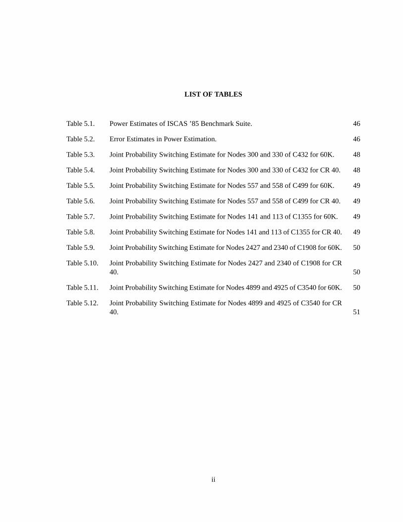
LIST OF TABLES

Table5.1. PowerEstimatesof ISCAS’85 BenchmarkSuite. 46

Table5.2. Error Estimatesin PowerEstimation. 46

Table5.3. JointProbabilitySwitchingEstimatefor Nodes300and330of C432for 60K. 48

Table5.4. JointProbabilitySwitchingEstimatefor Nodes300and330of C432for CR 40. 48


Table5.6. JointProbabilitySwitchingEstimatefor Nodes557and558of C499for CR 40. 49


Table5.8. JointProbabilitySwitchingEstimatefor Nodes141and113of C1355for CR40. 49





ii

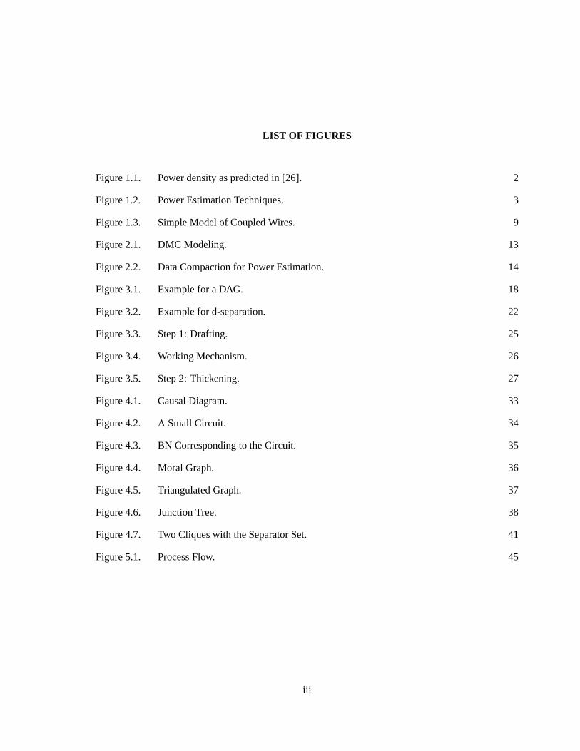
LIST OF FIGURES

Figure1.1. Powerdensityaspredictedin [26]. 2

Figure1.2. PowerEstimationTechniques. 3

Figure1.3. SimpleModelof CoupledWires. 9

Figure2.1. DMC Modeling. 13

Figure2.2. DataCompactionfor PowerEstimation. 14

Figure3.1. Examplefor aDAG. 18

Figure3.2. Examplefor d-separation. 22

Figure3.3. Step1: Drafting. 25

Figure3.4. WorkingMechanism. 26

Figure3.5. Step2: Thickening. 27

Figure4.1. CausalDiagram. 33

Figure4.2. A SmallCircuit. 34

Figure4.3. BN Correspondingto theCircuit. 35

Figure4.4. Moral Graph. 36

Figure4.5. TriangulatedGraph. 37

Figure4.6. JunctionTree. 38

Figure4.7. Two Cliqueswith theSeparatorSet. 41

Figure5.1. ProcessFlow. 45

iii

A COMPLETE PROBABILISTIC FRAMEW ORK FOR LEARNING INPUT MODELS FORPOWER AND CROSSTALK ESTIMATION IN VLSI CIRCUITS

Nirmal Munuswamy Ramalingam

ABSTRACT

Power disspiationis a growing concernin VLSI circuits. In this work we modelthedatadepen-

denceof power dissipationby learninganinput modelwhich we usefor estimationof bothswitching

activity andcrosstalkfor every nodein the circuit. We useBayesiannetworks to effectively model

thespatio-temporaldependencein theinputsandwe usetheprobabilisticgraphicalmodelto learnthe

structureof thedependency in the inputs. The learnedstructureis representative of the input model.

Sincewe learn a causalmodel, we can usea larger numberof independencieswhich guaranteesa

minimal structure.TheBayesiannetwork is convertedinto a moralgraph,which is thentriangulated.

Thejunctiontreeis formedwith its nodesrepresentingthecliques.Thenweuselogic samplingon the

junction treeandthesamplerequiredis really low. Experimentalresultswith ISCAS’85 benchmark

circuits show that we have acheived a very high compactionratio with averageerror lessthan2%.

As HSPICEwasusedthe resultsarethe mostaccuratein termsof delayconsideration.The results

canfurtherbeusedto predictthecrosstalkbetweentwo neighboringnodes.This predictionhelpsin

designingthecircuit to avoid theseproblems.

iv

CHAPTER 1

INTR ODUCTION

Moore’s Law which statesthatthenumberof transistorsperintegratedcircuit would doubleevery

coupleof yearshasbeenoneof the driving forcesfor the developmentteamsto breakdown these

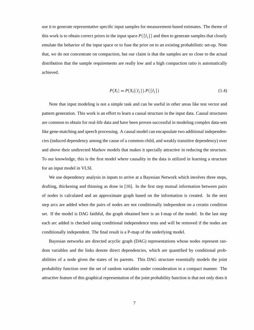
barriers. But the power consumedhasnot reducedandis not predictedto reduceeven in the nano-

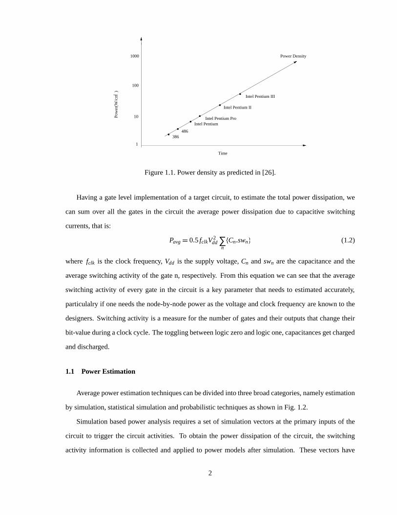
domain.Power densityor power dissipatedperunit areais increasingdueto thepackingof millions

of transistorsin a singlewafer (shown in Fig. 1.1.). Now, becauseof the increasein power density,

costincreasedfor highercooling andincreasedbatteryweight, not to forget the reductionin system

reliability. Designershadto make low power devicesto overcometheseproblems,andtheimpetuson

low-power design,saw an increasedattentionto power estimation. The total power consumedby a

circuit is calledtheaveragepower is givenby theformula,

Pavg � Pdynamic � Pshort � Pleakage (1.1)

CMOScircuitsconsistof a pull-up andpull-down network, whichhave a finite input fall/risetime

larger thanzero. During this short time interval, whenboth the pull-up andpull-down network are

conducting,acurrenticc flowsfrom supplyto ground,calledtheshort-circuitcurrent,resultingin short

circuit power.

Staticleakagepowerdissipiationcanbeattributedto reversebiasdiodeleakage,sub-thresholdleak-

age,gateoxide tunneling,leakagedueto hot carrierinjection,Gate-InducedDrain Leakage(GIDL),

andchannelpunchthrough.Note that this type of power dissipationdependson the logic statesof a

circuit thanits switchingactivites.

Themostimportantis thedynamiccomponentwhichconstitutesabout80%of theaveragepower.

Thecurrentid thatflowsdueto thecharginganddischargingof theparisiticcapacitanceduringswitch-

ing causesthepowerdissipationPdynamic.

1

Intel Pentium II

Intel Pentium ProIntel Pentium

486

Pow

er(W

/cm

386

Time

1

10

1000

100

2

)

Power Density

Intel Pentium III

Figure1.1.Powerdensityaspredictedin [26].

Having a gatelevel implementationof a target circuit, to estimatethe total power dissipation,we

can sum over all the gatesin the circuit the averagepower dissipationdue to capacitive switching

currents,thatis:

Pavg � 0 � 5 fclkV2dd ∑

n

�Cn � swn � (1.2)

where fclk is the clock frequency, Vdd is the supplyvoltage,Cn andswn arethe capacitanceandthe

averageswitchingactivity of thegaten, respectively. Fromthis equationwe canseethat theaverage

switchingactivity of every gatein the circuit is a key parameterthat needsto estimatedaccurately,

particulalryif oneneedsthenode-by-nodepower asthevoltageandclock frequency areknown to the

designers.Switchingactivity is a measurefor thenumberof gatesandtheir outputsthatchangetheir

bit-valueduringaclockcycle. Thetogglingbetweenlogic zeroandlogic one,capacitancesgetcharged

anddischarged.

1.1 Power Estimation

Averagepowerestimationtechniquescanbedividedinto threebroadcategories,namelyestimation

by simulation,statisticalsimulationandprobabilistictechniquesasshown in Fig. 1.2.

Simulationbasedpower analysisrequiresa setof simulationvectorsat theprimary inputsof the

circuit to trigger the circuit activities. To obtain the power dissipationof the circuit, the switching

activity information is collectedandappliedto power modelsafter simulation. Thesevectorshave

2

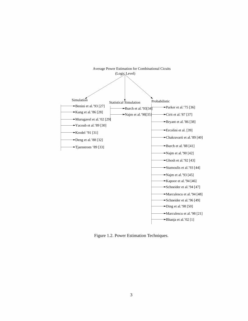
(Logic Level) Average Power Estimation for Combinational Cicuits

SimulationStatistical Simulation Probabilistic

Benini et al.’93 [27]

Kang et al.’86 [28]

Murugavel et al.’02 [29]

Yacoub et al.’89 [30]

Krodel ’91 [31]

Deng et al.’88 [32]

Tjarnstrom ’89 [33]

Burch et al.’93[34]

Najm et al.’98[35]

Parker et al.’75 [36]

Cirit et al.’87 [37]

Bryant et al.’86 [38]

Ercolini et al. [39]

Chakravarti et al.’89 [40]

Burch et al.’88 [41]

Najm et al.’90 [42]

Ghosh et al.’92 [43]

Stamoulis et al.’93 [44]

Najm et al.’93 [45]

Kapoor et al.’94 [46]

Schneider et al.’94 [47]

Marculescu et al.’94 [48]

Schneider et al.’96 [49]

Ding et al.’98 [50]

Marculescu et al.’98 [21]

Bhanja et al.’02 [1]

Figure1.2.PowerEstimationTechniques.

3

substantialimpacton thepower valuesbecausethepower dissipationreliesheavily on theswitching

activity. Eachvectorcausessomeenergy to bedissipatedandthetotal power is thesummationof the

energy of eachvectoranddividing over the total simulationtime. Usually thesetechniquesprovide

sufficient accuracy at theexpenseof largerunningtimesasthesemethodsusea very largesetof input

vectors.However themethodbecomesunrealisticto rely on whendoneon largecircuits.

Statisticalmethodsareusedin combinationwith simulationtechinquesin statisticalsimulation[41],

[42] to determinethestoppingcriterion. Thoughthesetechniquesareefficient in termsof thetime re-

quired,onehasto becarefulin modelingstatisticalpatternsat the inputsandcareshouldbetaken to

notgettrappedin a localminima.

In probabilistictechniquestheinput statistics(e.g.,switchingactivity of theinputs,signalcorrela-

tions,etc.) arefirst gatheredintermsof probabilitiesandthenthey arepropagated.They arefastand

moreadaptable,but involve anassumptionaboutjoint correlations.They provide sufficient accuracy

with alow computationaloverhead,but factorssuchasslew rates,glitch generationandpropagationare

difficult to capture.Anotherchallengein themethodis theability to accountfor internaldependencies

dueto reconvergentfanoutof thetargetcircuit.

1.2 Input Model

It is crucial thatthevectorsusedin simulationrepresentthetypical conditionsat which thepower

estimateissought.If thesimulationvectorsdonotcontaintheproperinstructionmix thepoweranalysis

resultwill beskewed.Regardlessof how thesimulationvectorsaregenerated,if wesimulatethecircuit

with only severalvectors,thepowerdissipationresultobtainedis not truthful becausethevectorlength

is tooshort.Mostpartof thecircuit is probablynotexercisedenoughto obtainactualtogglingactivites.

On theotherhandwe cansimulatethecircuit for a very largenumberof vectorsto obtainanaccurate

measureof the power dissipation. But is it necessarywastingcomputerresourcesto simulatethat

many vectors?How muchextra accuracy canwe acheive by simulatinga million vectorsversusonly

a thousandvectors?How do we know thatwe have simulatedenoughvectorlength?Whatis thecost

involved?

As saidin [5] thevectorcompactionproblemreducesthegapbetweensimulativeandnonsimulative

approaches.Theinputstatisticsthatmustbecapturedandthelengthof theinputsequenceswhichmust

4

beappliedaresomeof the issuesthatmustbetaken into consideration.Generatinga minimal length

sequencethatstaisfiestheabove conditionsis nota trivial task.Sovectorcompactionis thetechnique

by which a smallersetof vectorsis derivedfrom a largersetby a seriesof stepssuchthat thesmaller

derivedsetpreservestheoriginal statisticalpropertiesof thelargerinitial set.

Comingbackto thequestiononthelengthof thevectors,simulationmethodsareaccuratebut suffer

costandmemoryoverhead,which limit the sizeof the input vectorset to hundredsor thousandsof

vectors.But this resultsin inaccuracy in thepowerestimationprocessbecausethepowerconsumption

in digital circuitsis inputpatterndependant,thatis dependingon theinputvectorsappliedto thetarget

circuit very differentpower estimatesmaybeobtained.To obtainanaccuratepower estimate,a setof

inputsthat resemblethecharacteristicsof the datafor typical applicationsis required.So to acheive

thisgoalthevectorsethasasizeof millions of vectors.Vectorsof thesizeof hundredsor thousands,if

selectedrandomlyfrom thelargevectorsetmaynotbeabletocapturethetypicalbehavior andthusmay

leadto anunderestimationor overestimationof thepower consumedby thecircuit. Soour methodof

vectorcompactionsolvestheproblemby compactingthemillions of vectorsinto acharacteristicinput

setof a muchsmallerlength,yet statisticallyequivalentto theoriginal larger vector, thusprovding a

power estimatevery closeto thepower estimatedby thelargersequence.

Switching model of a VLSI circuit is a comprehensive representaionof switching behavior of

all the signalsin the circuit. At eachsignalwe storethe stateat time t andthe stateat time t � 1.

The dependency amongall the switchingvariablecanbe capturedasa joint Probabilitydistribution

function. One might look into switching model as a way to establishthe role of dataas inputs to

thecircuits. In essence,theswitchingmodelcapturesthedata-driven uncertaintyin VLSI circuits in

a comprehensive probabilisticframework. Needlessto saythat,modelinginputsbecomean integral

partof theswitchingmodel,eventhougha handfulof prior work in power or switchinganalysis,has

modeledinputsefficiently. Evenanalysisthatarevectordriven(simulationandstatisticalsimulation)

havemostlybecomeassumedinputpriorsasrandominputs.In thiswork,wetakealook into modeling

inputsthrougha causalgraphicalprobabilisticapproachwhich modelsinput spacein a compactway.

This inputmodelthencanbefusedwith avectorlessprobabilisticmodelor beusedto generatesamples

for statisticalor simulative approachesby a randomwalk in theprobabilsiticnetwork.

5

Notethattheswitchingmodelis extremelyrelevantof bothstaticanddynamiccomponentof power

asshown in Eq.1.3. In Eq.1.3,Pdg representsthedynamiccomponentof powerat theoutputof agate

g. The impactof dataon dynamiccomponentof power is encasulatedin α, the singletonswitching

activity. Thestaticcomponentof powerPsg is dominatedby Pleak� i , leakagelossin a leakagemodei. It

hasto benotedthateachleakagemodeis determinedby thesteadystatesignalsthateachtransistorin

thegatewould bein. For example,in a two input(sayA andB) NAND gate,thegatewould have four

dominantleakagemode(i=4: A@0B@0 � A@0B@1� A@1B@0 and A@1B@1). β is theprobabilityof each

modei. Probabilisticallyboth α andβ aresingletonprobabilityof switchingandjoint probabilityof

multiplesignalsin agaterespectively andaredependentontheinputdataprofile. Theswitchingmodel

is affectedby variousfactorssuchas the topologyof the circuit, the input statistics,the correlation

betweennodes,the gatetype, and the gatedelays,thus making the estimationprocessa complex

procedure.

Pt � ∑g Ptg � Pdg � Psg

� 0 � 5α fV2ddCload wire � ∑i Pleak� iβi

(1.3)

In this work, we focuson modelingthe inputsandgeneratea probabilisticstructureamongthe

inputsthatcanbeusedto studythebehaviors of internalnodes.Eventhoughestimationof singleton

switchinghasbeendiscussedin greatdepthandmany of theproceduresareinput driven (simulative

andstatisticalsimulative), inputsarestudiedin a limited setof works[2, 3, 57].

Eq. 1.4 demonstratesthe effect of input model. Let Xi be an intermediatesignalwhich could be

singletonswitchingvariablerepresentingswitchingstates(0t 10t � 0t 11t � 1t 10t and1t 11t ), of asignal

or Xi could be compositesignals(A,B) in a transistorstackand canhave compositestatesnamely

A � 0t 10t � B � 0t 10t . In estimatingXi, asshown in Eq. 1.4,we have two components,namelythe

setP�Xi � � I j � � , � I j � denotingtheprimary inputsof thecircuits,wherej is the jth input andP

� � I j � � a

prior probabilityof thetheinput space.Thefirst componentcanbeanalysedby probabilisticmeasure

consideringajoint pdf of theentiresignalsthroughaprobabilisticframework asin [43, 21, 1] or canbe

measured‘[28, 20] for specificinputpatterns.ThesecondcomponentP� � I j � � however, is importantfor

bothstimulus-sensitive approachandstimulus-freeapproachwherewe needto modelthedependency

structureof theinputsandtheneitheruseit in thejoint pdf of thesignalsfor probabilisticmethodsor

6

useit to generaterepresentative specificinputsamplesfor measurement-basedestimates.Thethemeof

thiswork is to obtaincorrectpriorsin theinputspaceP� � I j � � andthento generatesamplesthatclosely

emulatethebehavior of theinput spaceor to fusetheprior on to anexisting probabilisticset-up.Note

that,we do not concentrateon compaction,but our claim is that thesamplesaresocloseto theactual

distribution that thesamplerequirementsarereally low anda high compactionratio is automatically

achieved.

P�Xi � � P

�Xi � � I j � � � P � � I j � � (1.4)

Note that input modelingis not a simpletaskandcanbeusefulin otherareaslike testvectorand

patterngeneration.Thiswork is aneffort to learnacausalstructurein theinputdata.Causalstructures

arecommonto obtainfor real-lifedataandhavebeenprovensuccessfulin modelingcomplex data-sets

likegene-matchingandspeechprocessing.A causalmodelcanencapsulatetwo additionalindependen-

cies(induceddependency amongthecauseof acommonchild, andweaklytransitivedependency) over

andabove their undirectedMarkov modelsthatmakesit speciallyattractive in reducingthestructure.

To our knowledge,this is thefirst modelwherecausalityin thedatais utilized in learninga structure

for aninput modelin VLSI.

We usedependency analysisin inputsto arrive at a BayesianNetwork which involvesthreesteps,

drafting, thickeningandthinning asdonein [16]. In the first stepmutualinformationbetweenpairs

of nodesis calculatedand an approximategraphbasedon the information is created. In the next

steparcsareaddedwhenthepairsof nodesarenot conditionallyindependenton a ceratincondition

set. If the modelis DAG faithful, thegraphobtainedhereis an I-mapof the model. In the last step

eacharcaddedis checked usingconditionalindependencetestsandwill beremoved if thenodesare

conditionallyindependent.Thefinal resultis aP-mapof theunderlyingmodel.

Bayesiannetworks aredirectedacyclic graph(DAG) representationswhosenodesrepresentran-

dom variablesand the links denotedirect dependencies,which are quantifiedby conditionalprob-

abilities of a nodegiven the statesof its parents. This DAG structureessentiallymodelsthe joint

probability function over thesetof randomvariablesunderconsiderationin a compactmanner. The

attractive featureof thisgraphicalrepresentationof thejoint probabilityfunctionis thatnotonly doesit

7

makeconditionaldependency relationshipsamongthenodesexplicit but alsoservesasacomputational

mechanismfor efficientprobabilisticwalk generatingsamples.

ProbabilisticLogic Samplingis doneinsidethecliquesof thejunctiontreeto obtainthenecessary

samples.The stepsinvolved in formation the juction tree is the creationof a moral graph,and the

processis calledcompilation,thenthemoralgraphis triangulated.Thecliquesetis identifiedandthe

junctiontreeof cliquesis formed.Givena Bayesiannetwork, a moralgraphis obtainedby ’marrying

parents’,thatis addingundirectededgesbetweentheparentsof acommonchild node.Beforethisstep,

all thedirectionsin theDAG areremoved. Themoralgraphis saidto betriangulatedif it is chordal.

TheundirectedgraphG is calledchordalor triangulatedif every onof its cyclesof lengthgreaterthan

or equalto 4 posessesa chord[9], that is we addadditionallinks to the moral graph,so that cycles

longerthan3 nodesarebroken into cyclesof threenodes.The juntion treeis definedasa treewith

nodesrepresentingcliques(collectionof completelyconnectednodes)andbetweentwo cliquesin the

treeT thereis auniquepath.ProbabilisticLogic Samplingis amethodproposedby Henrion[56] which

employs astochasticsimulationapproachto make probabilisticinferencesin largemultiply connected

networks. If we representa Bayesiannetwork by a sampleof m deterministicscenarioss=1,2,.....m

andLs�x� is the truth of event x in scenarios, thenuncertaintyaboutx canberepresentedby a logic

sample.

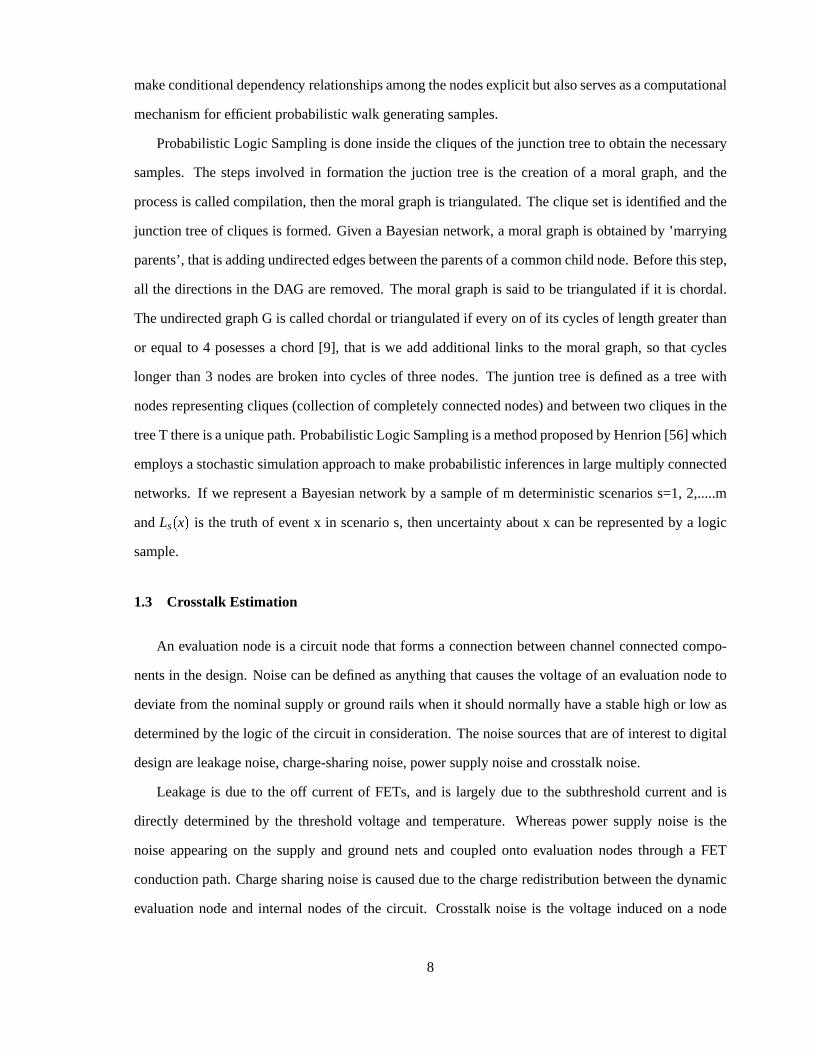
1.3 CrosstalkEstimation

An evaluationnodeis a circuit nodethat forms a connectionbetweenchannelconnectedcompo-

nentsin thedesign.Noisecanbedefinedasanything thatcausesthevoltageof anevaluationnodeto

deviatefrom thenominalsupplyor groundrails whenit shouldnormallyhave a stablehigh or low as

determinedby thelogic of thecircuit in consideration.Thenoisesourcesthatareof interestto digital

designareleakagenoise,charge-sharingnoise,power supplynoiseandcrosstalknoise.

Leakageis due to the off currentof FETs,andis largely due to the subthresholdcurrentandis

directly determinedby the thresholdvoltageand temperature.Whereaspower supply noiseis the

noiseappearingon the supply and groundnetsand coupledonto evaluationnodesthrougha FET

conductionpath.Chargesharingnoiseis causeddueto thechargeredistribution betweenthedynamic

evaluationnodeand internalnodesof the circuit. Crosstalknoiseis the voltageinducedon a node

8

R

R

C

C

i

m

Ci

L i

L

L

i

m

aggressor

victim

aggressor

victim

time

time

coupled noise

V

V

Figure1.3.SimpleModelof CoupledWires.

due to capacitive coupling to a switchingnodeof anothernet. It canalsobe saidas the capacitive

andinductive interferencecausedby thenodevoltagedevelopedon signallineswhenthenearbylines

changestate.It is a functionof theseparationbetweensignallines,thelineardistancethatsignallines

runparallelwith eachother. In today’s logic devicesthefasteredgerategreatlyincreasesthepossibility

of couplingor crosstalkbetweenthe signals.Crosstalkis oneof the issuesthat hamperdesignersto

acheivehigherspeeds,andsoit mustbereducedto levelswherenoextra time is requiredfor thesignal

to stabilize. The importanceto estimatecrosstalkcanbe further understoodaswe discussthe faults

thatit maybeinducedbetweentwo coupledinterconnects,namelytheaggressorandthevictim.

1. DelayFault

It occurswhensignalsof thetwo coupledinterconnectionsundergo oppositeswings.This fault

affectsthegatedelaywhich inturncanchangethecritical pathdelayandcauseglitches.

2. Logic Fault

Herea logic error occurswhen the voltageinducedin the victim interconnectby the aggres-

sor interconnectis greaterthana threshold.This causesthe circuit malfunctionwhenthe risk

toleranceboundis exceeded.

3. Noise-inducedRaceFailures

9

Theracefailuresareaconsequenceof thedelayfault. Thechangein thedelaycausesahold-time

violation,commonlynoticedin pipelinedcircuits.

In a simplifiedmodelasshown in Fig. 1.3.,couplingcanbeconsideredbetweenthetwo linesasa

capacitivevoltagedivider. HigherintegrationcauseslargermutualcapacitanceCm andsmallerintrinsic

capacitanceCi of a line, both worseningcrosstalk. The sameis valid for the inductive couplingas

the mutual inductanceLm grows significantly in denserstructures.Taking the output resistancesR

andthe input capacitancesof the receiving circuits into accountthemodelshows a crosstalkvoltage

propotionalto thecouplingwire length.

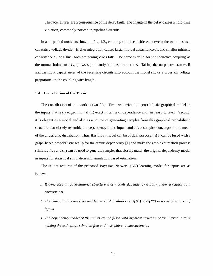
1.4 Contrib ution of the Thesis

The contribution of this work is two-fold. First, we arrive at a probabilisticgraphicalmodel in

the inputsthat is (i) edge-minimal(ii) exact in termsof dependenceand(iii) easyto learn. Second,

it is elegantasa modelandalsoasa sourceof generatingsamplesfrom this graphicalprobabilistic

structurethatcloselyresemblethedependency in theinputsanda few samplesconvergesto themean

of theunderlyingdistribution. Thus,this input-modelcanbeof dualpurpose:(i) It canbefusedwith a

graph-basedprobabilisticsetup for thecircuit dependency [1] andmake thewholeestimationprocess

stimulus-freeand(ii) canbeusedto generatesamplesthatcloselymatchtheoriginaldependency model

in inputsfor statisticalsimulationandsimulationbasedestimation.

The salient featuresof the proposedBayesianNetwork (BN) learningmodel for inputs are as

follows.

1. It generatesan edge-minimalstructure that modelsdependencyexactly under a causaldata

environment

2. Thecomputationsare easyand learningalgorithmsare O(N2 � to O(N4) in termsof numberof

inputs

3. Thedependencymodelof the inputscanbefusedwith grphical structure of the internal circuit

makingtheestimationstimulus-freeandinsensitiveto measurements

10

4. The dependencymodelcan be probabilistically efficiently sampledsuch that samplesclosely

emulatethedependenciesin theinputsfor statisticalsimulationandsimulationbasedestimation

process.

5. The performancethat is seenthe ISCAScircuits generatesa maximumerror of 1.8% with a

compressionratio up to 300.

11

CHAPTER 2

RELATED WORK

2.1 Vector Compaction

Thepioneeringwork in thisfield doneby Marculescuet. al, [2]-[7], have approachedtheproblem

first usingaStochasticSequencialMachineandlaterby usingMarkov Networks.

In [3] theapproachto tacklethis problemwasbasedon thestochasticsequentialmachines(SSMs)

theoryandemphasiswason thoseaspectsrelatedto Moore-typemachines.Finite Automataaremath-

ematicalmodelsfor varioussystemswith a finite numberof states.Thesemodelsacceptparticular

inputs,at discretetime intervals andemit outputsaccordingly. The automatais consideredto show

stochaticbehavior asthe currentstateof the machineandthe input given determineaccordinglythe

next stateandtheoutputof theautomaton.Heretheauthorssynthesizefirst a stochasticmachinethat

is probabilisticallyequivalentto theinitial sequence.Then,by applyingrandomlygeneratedinputsto

thestochasticmachine,a randomwalk throughthestatesof thetransitiongraphis doneanda shorter

sequnceis generated.The ideaproposedin this paperis that the automatonwhenin statexi andre-

ceiving input n, canmove into a new statex j with a positive probability p�xi � n� . Thebasictaskis of

synthesizinganSSMwhich is capableof generatingconstrainedinput sequencesanduseit in power

estimation.Themethodproposedfor power estimationof a target circuit for a given input vectorse-

quenceof lengthL0 is to derive a probabilisticmodelbasedon SSMsandgeneratea shortersequence

L, which is usedto calculatethepower of thetargetcircuit.

The methodusedin [3] hassomelimitations asthe authorsuseprobabilisticautomatatheoryto

synthesisestochasticmachines,wherethe compactiontechniquebecomesa multi-stepprocess.An

initial passthroughthesequenceis performedfirst to extractthestatisticsneededandthenthestochas-

tic machineis synthesisedto generatethenew compactedsequence.Thismethodbearsahugeloadon

computermemoryandtime especiallywhenvectorsequencesarevery large. Also, somedistributions

12

Intial SequenceL0 DMC Modelling Generate Compacted

Sequence L

Compacted Sequence L<L0

Power EstimationPower Estimation

Comparison

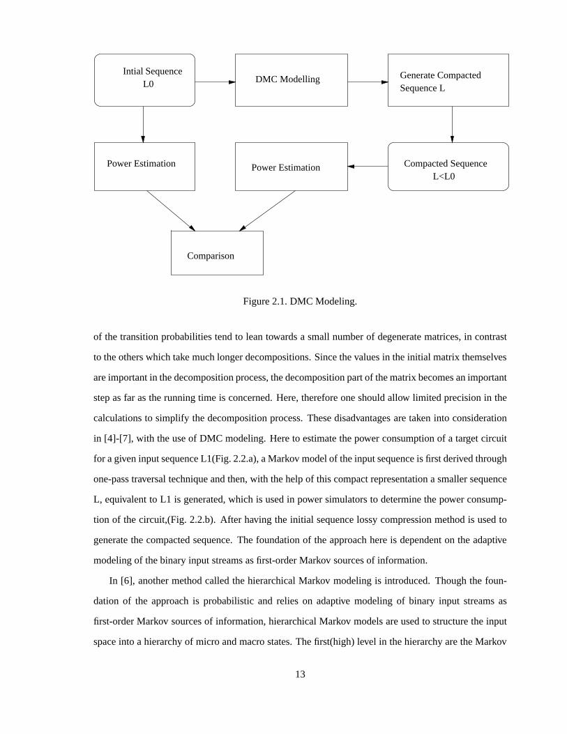
Figure2.1.DMC Modeling.

of the transitionprobabilitiestendto leantowardsa smallnumberof degeneratematrices,in contrast

to theotherswhich take muchlongerdecompositions.Sincethevaluesin theinitial matrix themselves

areimportantin thedecompositionprocess,thedecompositionpartof thematrixbecomesanimportant

stepasfar astherunningtime is concerned.Here,thereforeoneshouldallow limited precisionin the

calculationsto simplify thedecompositionprocess.Thesedisadvantagesaretaken into consideration

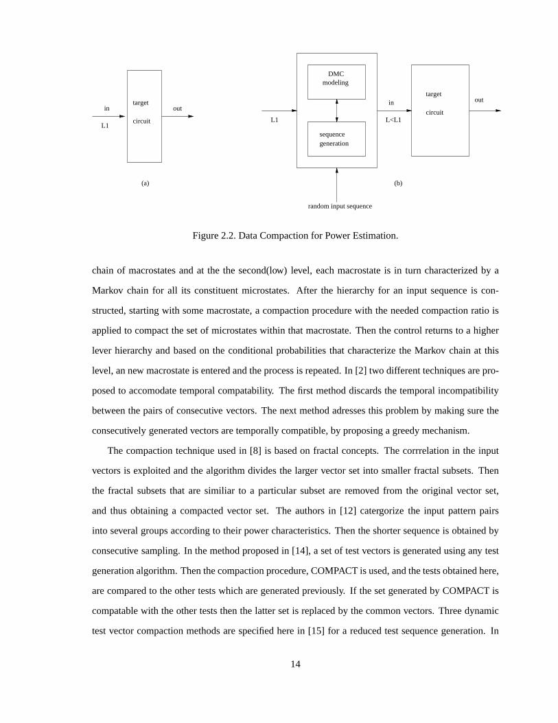
in [4]-[7], with theuseof DMC modeling.Hereto estimatethepower consumptionof a targetcircuit

for agiveninputsequenceL1(Fig.2.2.a),aMarkov modelof theinputsequenceis first derivedthrough

one-passtraversaltechniqueandthen,with thehelpof this compactrepresentationasmallersequence

L, equivalentto L1 is generated,which is usedin power simulatorsto determinethepower consump-

tion of thecircuit,(Fig.2.2.b). After having the initial sequencelossycompressionmethodis usedto

generatethecompactedsequence.The foundationof theapproachhereis dependenton theadaptive

modelingof thebinaryinput streamsasfirst-orderMarkov sourcesof information.

In [6], anothermethodcalledthehierarchicalMarkov modelingis introduced.Thoughthe foun-

dation of the approachis probabilisticand relies on adaptive modelingof binary input streamsas

first-orderMarkov sourcesof information,hierarchicalMarkov modelsareusedto structuretheinput

spaceinto a hierarchyof micro andmacrostates.Thefirst(high)level in thehierarchyaretheMarkov

13

in outtarget

circuitL1

DMCmodeling

sequencegeneration

intarget

circuit

out

random input sequence

L1 L<L1

(a) (b)

Figure2.2.DataCompactionfor PowerEstimation.

chainof macrostatesandat the the second(low) level, eachmacrostateis in turn characterizedby a

Markov chain for all its constituentmicrostates.After the hierarchyfor an input sequenceis con-

structed,startingwith somemacrostate,a compactionprocedurewith theneededcompactionratio is

appliedto compactthesetof microstateswithin thatmacrostate.Thenthecontrol returnsto a higher

lever hierarchyandbasedon the conditionalprobabilitiesthat characterizethe Markov chainat this

level, annew macrostateis enteredandtheprocessis repeated.In [2] two differenttechniquesarepro-

posedto accomodatetemporalcompatability. Thefirst methoddiscardsthe temporalincompatibility

betweenthepairsof consecutive vectors.Thenext methodadressesthis problemby makingsurethe

consecutively generatedvectorsaretemporallycompatible,by proposingagreedymechanism.

The compactiontechniqueusedin [8] is basedon fractal concepts.The corrrelationin the input

vectorsis exploited andthe algorithmdividesthe larger vectorsetinto smallerfractal subsets.Then

the fractal subsetsthat are similiar to a particularsubsetare removed from the original vector set,

and thus obtaininga compactedvector set. The authorsin [12] catergorize the input patternpairs

into severalgroupsaccordingto their power characteristics.Thentheshortersequenceis obtainedby

consecutive sampling.In themethodproposedin [14], a setof testvectorsis generatedusingany test

generationalgorithm.Thenthecompactionprocedure,COMPACT is used,andthetestsobtainedhere,

arecomparedto theothertestswhich aregeneratedpreviously. If thesetgeneratedby COMPACT is

compatablewith theotherteststhenthe lattersetis replacedby thecommonvectors.Threedynamic

testvectorcompactionmethodsarespecifiedherein [15] for a reducedtestsequencegeneration.In

14

all themethodsthesequencegeneratedfrom anAutomaticTestPatternGenerator(ATPG) for a single

fault, is assignedspecificvaluesfor unspecifiedprimary inputs. In the first methodcalled the Best

RandomFill, all theunspecifiedprimaryinputsaregivenfinite numberof randomnumbers,andeach

onesimulatedto determinewhich detectsthemostnumberof faults.Thenext methodcalledtheBest

RandomFill 2 hasslight modificationsof theprevious algorithm. Hereeachfault is given a weight,

theharderonegettingthehighest,andthefill which getsthehighestnumberof harder-to-find faults

is selected.This algorithmis mademoreeffective by not producingsimilar randomfills. The next

methodknown astheWeightedDeterministicFill, givesdeterministicvaluesto theunspecifiedinputs.

First the numberof stuck-at-0andstuck-at-1faultspropogatedis found. Thenthe gatewith highest

numberof faultspassedto it is foundandits inputsareassignedby backtrackingto primaryinputs.

2.2 CrosstalkEstimation

In [24] theauthorsaim to find thesetof interconnectionpairswhich will not posecrosstalkprob-

lemsduring normaloperationof the circuit. They statethat the effect of the environmentuponany

target circuit, morespecificallyon its layout that it is designedto work, andunderconditonswhich

areassumedto beknown to thedesignercanbemodeledby capturingtheinput patterndependencies.

Taking into accountthis typeof modelingcanresultin a muchsimplercircuit thanwhenit designed

discardingtheinputpatterncorrelations.In [25] thenecessityto consideron-chipsimultaneousswitch-

ing noise(SSN)is dealtwith, particularlywhendeterminingthepropagationdelayof a CMOSlogic

gatein ahighspeedsynchronousCMOSICs. Thepaperpresentsanalyticalexpressionswhichcharac-

terizeon-chipSSNandalsotheeffect of SSNon thepropagationdelayandoutputvoltageof a logic

gate.In [51] theauthorsextracttheelectricalparametersfor a basesetof adjacentwire configuration.

This stepis doneonly oncedependenton thethetechnology, thenthegeometryof thecompletechip

routing spacesis extracted.The adjacency lengthsbetweenthechosenvictim andits agressorscon-

sideringthewire widths andspacingsis calculated.Thenthe effective ouputresistancesinfluencing

thesignalslopesandtheamountof couplednoiseis determined.Finally theswitchingtimesof victim

andagressorlines from thechip’s timing reportis readandall timing-uncriticalwire adjacenciesare

disregarded. A comprehensive methodolgyfor understandingandanalyzingthe noiseimmunity of

digital integratedcircuitsis presentedin [52]. A noiseclassificationbasedonnoiselevel relative to the

15

supplyandgroundrails is introduced.A noisestability metricasa practicalformal basisfor ensuring

noiseimmunity is described.A staticnoiseanlaysisapproachis alsoexplained,which canbe used

asa techniquefor identifying all possibleon-chip functional failureswithout full patterndependent

dynamicalsimulation.TheHarmony is thenusedto combinestatictiming analysisandreducedorder

modellingwith transistor-level analysis.

16

CHAPTER 3

LEARNING BAYESIAN NETWORKS

3.1 BayesianNetworks

BayesianNetwork is agraphicalprobabilisticmodelbasedontheminimalgraphicalrepresentation

of theunderlyingjoint probability function. It canbedefinedasa directedacyclic graph(DAG) with

a probability table for eachnodeandthe nodesin the network representthe propositional(random)

variablesin thedomainandthearcsbetweenthenodesrepresentthedependency relationshipamong

thevariables.Beforedelvingdeepinto thedefinitionlet usdiscusssomebasicconcepts.

Definition: Let E andF beeventssuchthatP�F �� 0. Thentheconditionalprobabilityof E given

F, is givenby

P�E � F � � P

�E � F �P�F � (3.1)

Bayes’ Theorem : The Bayestheoremdevolepedby ThomasBayesin 1763forms the basisof

BayesianNetworks.

Definition: Giventwo eventsE anfF suchthatP�E �� 0 andP

�F �� 0, then

P�E � F � � P

�E � F � P � E �

P�F � (3.2)

Proof: we useEq.3.1to derive theBayestheorem.

P�E � F � � P � E � F �

P � F � andsimilarly we canwrite,

P�F � E � � P � F � E �

P � E � .

Multiplying theseequalitiesby thedenominator, we get,

P�E � F � P � F � � P

�F � E � P � E � asP

�E � F � � P

�F � E � , so

P�E � F � � P � E �F � P � E �

P � F � .

Somebasicdefinitionsrelatedto Bayesiannetworksareasgivennext:

17

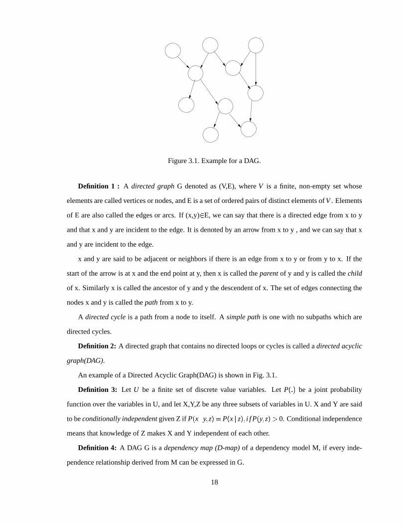
Figure3.1.Examplefor aDAG.

Definition 1 : A directedgraph G denotedas (V,E), whereV is a finite, non-emptyset whose

elementsarecalledverticesor nodes,andE is asetof orderedpairsof distinctelementsof V. Elements

of E arealsocalledtheedgesor arcs. If (x,y) � E, we cansaythat thereis a directededgefrom x to y

andthatx andy areincidentto theedge.It is denotedby anarrow from x to y , andwe cansaythatx

andy areincidentto theedge.

x andy aresaidto beadjacentor neighborsif thereis an edgefrom x to y or from y to x. If the

startof thearrow is at x andtheendpoint at y, thenx is calledtheparentof y andy is calledthechild

of x. Similarly x is calledtheancestorof y andy thedescendentof x. Thesetof edgesconnectingthe

nodesx andy is calledthepath from x to y.

A directedcycleis a pathfrom a nodeto itself. A simplepath is onewith no subpathswhich are

directedcycles.

Definition 2: A directedgraphthatcontainsnodirectedloopsor cyclesis calledadirectedacyclic

graph(DAG).

An exampleof aDirectedAcyclic Graph(DAG) is shown in Fig. 3.1.

Definition 3: Let U be a finite set of discretevalue variables. Let P� � � be a joint probability

functionover thevariablesin U, andlet X,Y,Z beany threesubsetsof variablesin U. X andY aresaid

to beconditionallyindependentgivenZ if P�x � y� z� � P

�x � z� � i f P

�y� z�� 0. Conditionalindependence

meansthatknowledgeof Z makesX andY independentof eachother.

Definition 4: A DAG G is a dependencymap(D-map)of a dependency modelM, if every inde-

pendencerelationshipderivedfrom M canbeexpressedin G.

18

Definition 5: A DAG G is an independencemap (I-map) of a dependency model M, if every

independencerelationshipderivedfrom G correspondsto avalid conditionalindependencerelationship

in M.

Definition 6: A DAG G is a minimal I-mapof a dependency modelM if it is an I-mapof M and

deletionof any of its edgesfrom G destroys theindependencerelationof M.

Definition 7: A DAG G is bothaD-mapandanI-mapof thedependency modelM, if it is aperfect

map(P-map)of M.

Definition 8: A DAG G is called a BayesianNetworkof a probability function P on a set of

variablesU, if G is aminimal I-mapof P.

Also a Bayesiannetwork is a directedacyclic graph(DAG) representationof theconditionalfac-

toringof a joint probabilitydistribution. Any probabilityfunctionP�x1 �� xn � canbewritten as1

P�x1 �� xN � � P

�xn � xn 1 � xn 2 �� x1 � P � xn 1 � xn 2 � xn 3 �� x1 � �� P � x1 � (3.3)

This expressionholdsfor any orderingof therandomvariables.Therepresentationandinfernceusing

this equationbecomesvery tediouswhenn becomesvery large. In mostapplications,a variableis

usuallynot dependenton all othervariables.Therearelots of conditionalindependenciesembedded

amongthe randomvariables. The above equationdoesnot considertheseindependecies,but these

dependenciescanbeusedto reordertherandomvariablesandto simplify theconditionalprobabilities.

P�x1 �� xN � � ΠvP

�xv �Pa

�Xv �� (3.4)

wherePa�Xv � arethe parentsof the variablexv, representingits direct causes.This factoringof the

joint probability functioncanbe representedasa directedacyclic graph(DAG), with nodes(V) rep-

resentingtherandomvariablesanddirectedlinks (E) from theparentsto thechildren,denotingdirect

dependencies.

Definition 9: A Bayesiannetwork G of adistribution Pdeterminesasetof independencerelations.

Theseindependencerelationsin turn mayentailothers,in thesensethatevery probabilitydistribution

having independencerelationswill alsohave further independencerelationsasexplainedin [18]. In1Probabilityof theeventXi � xi will bedenotedsimplyby P � xi or by P � Xi � xi .

19

otherwordsG of thedistribution P maynot representall theconditionalindependencerelationsof P.

But, whenG canactuallyrepresentall theconditionalindependencerelationsof P, thenP andG are

faithful to eachother. In [10], G is calledaperfectmapof PandP is calledtheDAG-Isomorphof G.

Definition : A dependency modelM is saidto becausalor a DAG isomorphif thereis a DAG D

thatis a perfectmapof M relative to d-separation,i.e.,

I�X � Z � Y � M !#"%$ X � Z � Y � D (3.5)

Theorem : A necessarycondition for a depndency model M to be a DAG isomorphis that

I�X � Z � Y � M satisfiesthefollowing independentaxioms.

Symmetry:

I�X � Z � Y � !#" I

�Y � Z � X � (3.6)

Composition/Decomposition:

I�X � Z � Y & W � !#" I

�X � Z � Y � & I

�X � Z � W � (3.7)

Intersection:

I�X � Z & W� Y � & I

�X � Z & Y � W � �'" I

�X � Z � Y & W � (3.8)

Weakunion:

I�X � Z � Y & W � �'" I

�X � Z & W� Y � (3.9)

Contraction:

I�X � Z & Y � W � & I

�X � Z � Y � �'" I

�X � Z � Y & W � (3.10)

WeakTransitivity:

I�X � Z � Y � & I

�X � Z & γ � Y � �'" I

�X � Z � γ � orI

�γ � Z � Y � (3.11)

Chordality :

I�α � γ & δ � β � & I

�γ � α & β � δ � �'" I

�α � γ � β � orI

�α � δ � β � (3.12)

20

Why BayesianNetworks?

1. BayesNetworksprovide anaturalrepresentationfor conditionalindependence.

2. Topologyandthe Conditionalprobability tablesprovide a compactrepresentationof the joint

distribution.

3. Bayesiannetworksaregenerallyeasyto construct.An equivalentrepresentationnamelyMarkov

networksaretediousto constructandmoreover they areundirectionalandinferencingbecomes

moretimeandmemoryconsuming.

4. Inferencein Bayesnetworks is easier, for examplepolytreeinferencingis anNP hardproblem

on generalgraphs.

5. Learningof Bayesiannetworksprovide acompactrepresentationof thedata.Having this repre-

sentationof thedata,inferencingis easierandfaster.

3.2 Learning

In a Bayesiannetwork, the graph,called the DirectedAcyclic Graph(DAG), is the structureof

the BayesianNetwork, andthe conditionalprobability distribution is calledthe parameter. Both the

parameterandthestructurecanbeseperatelylearnedfrom thedata.While learningtheparameter, we

assumethat we know the structureof the DAG, but in structurelearningwe startwith only a setof

randomvariableswith unknown relative frequency distribution. Learningstructurecanalsobe done

with missingdataitems,andhiddenvariablesandalsoin thecaseof continuousvariablesasdiscussed

in [11]. Therearetwo majormethodsto Bayesiannetwork learning,namelysearchandscoringmethod

anddependency analysismethods.In thisexperimentweareusingthedependency analysismethodto

learnthebayesiannetwork structurefrom data.Theinput to learntheBayesiannetwork is a database

table. Eachnodein the network is a representative of the fields in the database.Eachrecordin the

givendatabaseis a completeinstantiationof therandomvariables.We assumethat thedatabasetable

hasdiscretevaluesandthedatasetis completewith nomissingvalues.Also, thevolumeof thedataset

shouldbe large enoughsothat reliableCI testscouldbeperformed.In dependency analysismethod,

conditional independenceplay an importantrole, and by using the conceptof direction dependent

21

X Y

Z

A

B

C

Figure3.2.Examplefor d-separation.

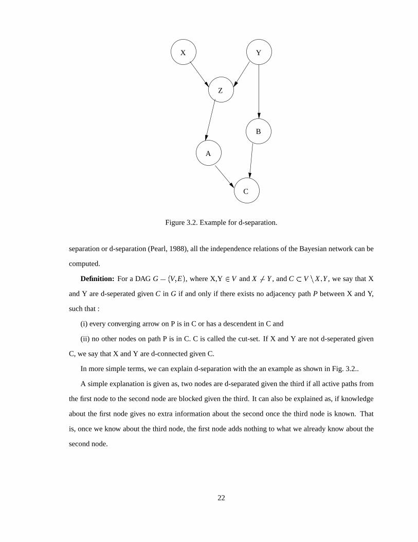
separationor d-separation(Pearl,1988),all theindependencerelationsof theBayesiannetwork canbe

computed.

Definition: For a DAG G � �V � E � , whereX,Y � V andX �� Y, andC ( V ) X � Y, we saythatX

andY ared-seperatedgivenC in G if andonly if thereexistsno adjacency pathP betweenX andY,

suchthat:

(i) every converging arrow on P is in C or hasadescendentin C and

(ii) no othernodeson pathP is in C. C is calledthecut-set.If X andY arenot d-seperatedgiven

C, we saythatX andY ared-connectedgivenC.

In moresimpleterms,wecanexplaind-separationwith theanexampleasshown in Fig. 3.2..

A simpleexplanationis givenas,two nodesared-separatedgiventhethird if all active pathsfrom

thefirst nodeto thesecondnodeareblockedgiventhethird. It canalsobeexplainedas,if knowledge

aboutthefirst nodegivesno extra informationaboutthesecondoncethe third nodeis known. That

is, oncewe know aboutthethird node,thefirst nodeaddsnothingto whatwe alreadyknow aboutthe

secondnode.

22

In the exampe,Fig. 3.2. Z is d-separatedfrom B, given Y asall pathsfrom X to Y areblocked

givenZ. Also Z is notd-separatedor it is d-connectedfrom B givenC asall pathsbetweenZ andB are

notblockedasthereexistsapaththroughY.

If two nodesaredependent,thenthe knowledgeof the valueof onenodewill give us somein-

formationof the value of the othernode. This informationgain can be measuredby usingmutual

information.Thereforetheknowledgeof mutualinformationcantell usaboutthedependency relation

betweentwo nodes.Themutualinformationof two nodesXi,Xj is expressedas:

I�Xi � Xj � � ∑

xi � xj

P�xi � x j � log

P�xi � x j �

P�xi � P � x j � (3.13)

andtheconditionalmutualinformationis definedas

I�Xi � Xj � C � � ∑

xi � xj � cP�xi � x j � c� log

P�xi � x j � c�

P�xi � c� P � x j � c� (3.14)

whereC is a setof nodes.WhenI�Xi � Xj � is smallerthana certainthresholdε, we saythatXi � Xj

aremarginally independent.WhenI�Xi � Xj � C � is smallerthanε, we saythatXi � Xj areconditionally

independentgivenC.

3.3 Algorithm for Learning BayesianNetwork Given NodeOrdering

The algorithm is the work of Cheng et.al [16] which constructsa Bayesiannetwork basedon

dependency analysisfrom a databasetable as input. A similar work is the Chow-Liu algorithmas

explainedin [10].

Therearethreesteps,thatthealgorithmperforms,namelydrafting,thickeningandthinning. In the

first stepa draft is createdbasedon themututalinformationof eachpair of nodes.In thesecondstep

known asthickening,arcsareaddedwhenthepair of nodesarenot conditionallyindependentbased

on a certainconditionset. We getan I-mapat theendof this stepwhich is of theunderlyingdepen-

dency modelgiven it is DAG faithful. In the laststepthearcsaddedin theprevioussteparechecked

usingconditionalindependencetestsandthe arc will be removed if any two nodesarecondtionally

independent.Soat theendof thethird stepwegetaperfectmapof themodelwhenit is DAG faithful.

23

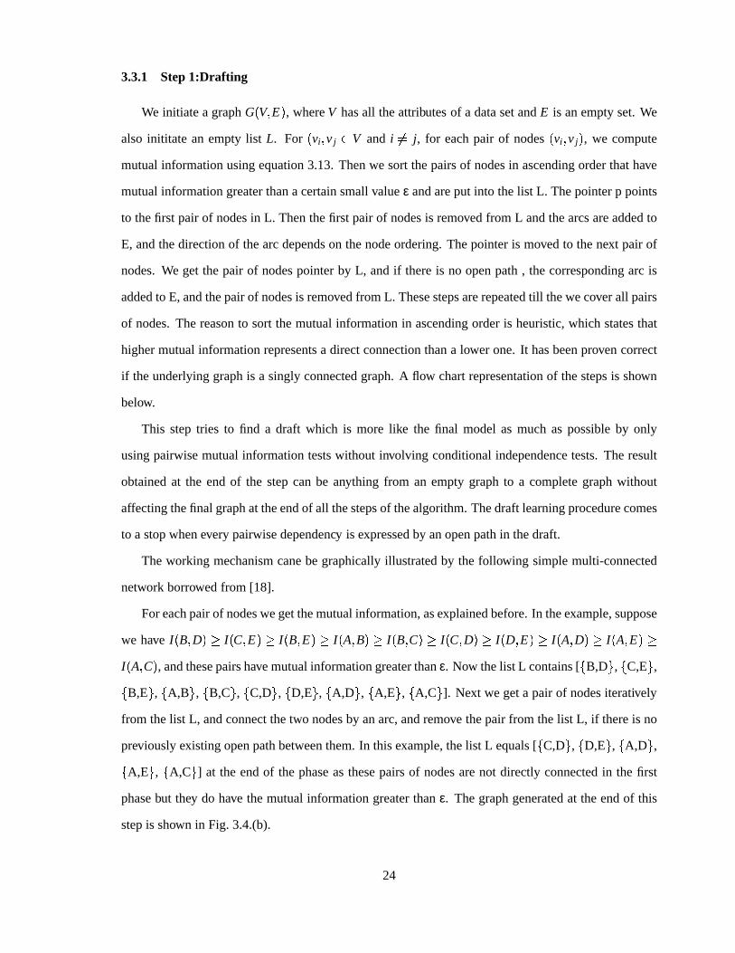
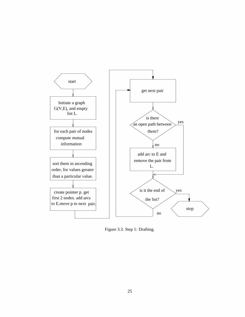
3.3.1 Step1:Drafting

We initiate a graphG�V � E � , whereV hasall theattributesof a datasetandE is anemptyset.We

also inititate an empty list L. For�vi � v j � V and i �� j, for eachpair of nodes

�vi � v j � , we compute

mutualinformationusingequation3.13. Thenwe sort thepairsof nodesin ascendingorderthathave

mutualinformationgreaterthanacertainsmallvalueε andareput into thelist L. Thepointerp points

to thefirst pair of nodesin L. Thenthefirst pair of nodesis removedfrom L andthearcsareaddedto

E, andthedirectionof thearcdependson thenodeordering.Thepointeris movedto thenext pair of

nodes.We get thepair of nodespointerby L, andif thereis no openpath, thecorrespondingarc is

addedto E, andthepairof nodesis removedfrom L. Thesestepsarerepeatedtill thewecoverall pairs

of nodes.Thereasonto sort themutualinformationin ascendingorderis heuristic,which statesthat

highermutualinformationrepresentsa directconnectionthana lower one. It hasbeenprovencorrect

if theunderlyinggraphis a singly connectedgraph.A flow chartrepresentationof thestepsis shown

below.

This steptries to find a draft which is more like the final model as much as possibleby only

usingpairwisemutualinformationtestswithout involving conditionalindependencetests.Theresult

obtainedat the endof the stepcanbe anything from an empty graphto a completegraphwithout

affectingthefinal graphat theendof all thestepsof thealgorithm.Thedraft learningprocedurecomes

to a stopwhenevery pairwisedependency is expressedby anopenpathin thedraft.

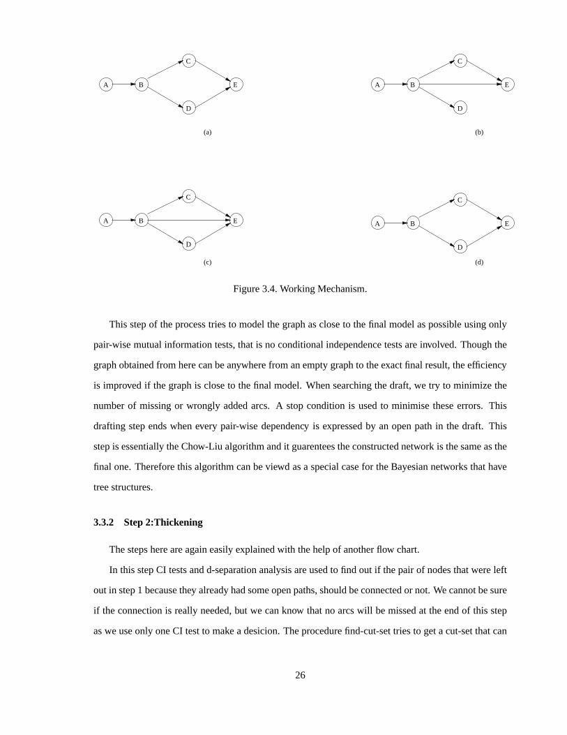
Theworking mechanismcanebegraphicallyillustratedby the following simplemulti-connected

network borrowedfrom [18].

For eachpairof nodeswegetthemutualinformation,asexplainedbefore.In theexample,suppose

we have I�B � D �+* I

�C � E �+* I

�B � E �,* I

�A � B�,* I

�B � C �,* I

�C � D �+* I

�D � E �,* I

�A � D �,* I

�A � E �,*

I�A � C � , andthesepairshavemutualinformationgreaterthanε. Now thelist L contains[ � B,D � , � C,E� ,

� B,E� , � A,B � , � B,C� , � C,D� , � D,E� , � A,D � , � A,E � , � A,C � ]. Next we geta pair of nodesiteratively

from thelist L, andconnectthetwo nodesby anarc,andremove thepair from thelist L, if thereis no

previously existingopenpathbetweenthem.In thisexample,thelist L equals[ � C,D� , � D,E� , � A,D � ,� A,E � , � A,C � ] at the endof the phaseasthesepairsof nodesarenot directly connectedin the first

phasebut they do have themutualinformationgreaterthanε. Thegraphgeneratedat theendof this

stepis shown in Fig. 3.4.(b).

24

is it the end of

start

yes

no

no

yes

for each pair of nodes

G(V,E), and empty

create pointer p. get first 2 nodes. add arcs

stopto E.move p to next pair.

order, for values greatersort them in ascending

than a particular value.

compute mutual information

Initiate a graph

list L.

get next pair

is there

an open path between

them?

L.remove the pair from

add arc to E and

the list?

Figure3.3.Step1: Drafting.

25

(a) (b)

(c) (d)

A B

C

D

E A B

C

D

E

A B

C

D

EA B

C

D

E

Figure3.4.WorkingMechanism.

This stepof theprocesstriesto modelthegraphascloseto thefinal modelaspossibleusingonly

pair-wisemutualinformationtests,that is no conditionalindependencetestsareinvolved. Thoughthe

graphobtainedfrom herecanbeanywherefrom anemptygraphto theexactfinal result,theefficiency

is improved if thegraphis closeto thefinal model. Whensearchingthedraft, we try to minimizethe

numberof missingor wrongly addedarcs. A stopcondition is usedto minimisetheseerrors. This

drafting stependswhenevery pair-wise dependency is expressedby an openpathin the draft. This

stepis essentiallytheChow-Liu algorithmandit guarenteestheconstructednetwork is thesameasthe

final one.Thereforethis algorithmcanbeviewd asa specialcasefor theBayesiannetworksthathave

treestructures.

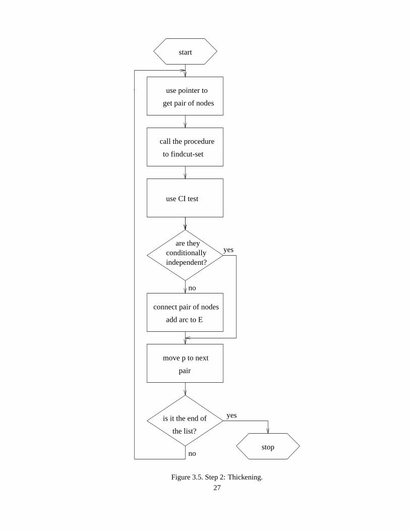
3.3.2 Step2:Thickening

Thestepshereareagaineasilyexplainedwith thehelpof anotherflow chart.

In thisstepCI testsandd-separationanalysisareusedto find out if thepair of nodesthatwereleft

out in step1 becausethey alreadyhadsomeopenpaths,shouldbeconnectedor not. Wecannotbesure

if theconnectionis really needed,but we canknow thatno arcswill bemissedat theendof this step

aswe useonly oneCI testto make adesicion.Theprocedurefind-cut-settriesto getacut-setthatcan

26

are they

connect pair of nodes

is it the end of

the list?

stop

yes

no

yes

no

use CI test

use pointer to

move p to next

get pair of nodes

add arc to E

pair

start

call the procedure

to findcut-set

conditionallyindependent?

Figure3.5.Step2: Thickening.

27

d-seperatethetwo nodes,andthis is donefor everypairof nodes.Thenit usesaCI testto seeif thetwo

nodesareindependentconditionalon thecut-set.Thearc is addedif thenodesarenot conditionally

independent.Somearcscanbe wrongly added,becausesomeneededarcsmay be missingandthey

hinderfindingapropercut-set.

Thegraphafter thesecondstepis shown in Fig. 3.4.(c). Arc (D,E) is addedbecauseD andE are

not independentgivenB, which is thesmallestcut-setbetweenD andE. Also, arc(A,C) is not added

becausetheconditionalindependencetestsshow thatA andC areindependentgivenB. Similarly, for

thesamereasonswedonotaddarcs(A,D), (C,D), (A,E). Fromthegrpahwecanalsoseethatafterthis

stpethegraphobtainedis anI-mapof theunderlyingmodel.

3.3.3 Step3: Thinning

For the two nodesunderconsideration,if thereareotherpaths,otherthanthearc, thenthearc is

temporarilyremovedfrom E, andtheprocedureis calledagainto find a cut-setthatcand-seperatethe

two nodes.Now giventhacut-settheCI testis doneto find outwhetherthetwo nodesareconditionally

independent.If so, thearc is permanentlyremoved or elseit is addedback. This stepis basicallyto

find thearcswhich maybebeenwrongly addedin theprevioussteps.Herewe alsomake sureall the

addesarcsareneededandthereareno extra ones,by usingonly oneCI test. Sincethecurrentgraph

hadbecomeanI-mapat theendof thepreviousstep,we canbesurethatthedescionto remove arcsis

correct. In this step,we try to find thatanarcconnectinga pair of nodesarealsoconnectedby other

paths.This is donebecauseit is possiblethat thedependency betweenpair of nodescouldnot bedue

to thedirectarc. Thenthealgorithmremovesthis arcandusestheprocedureto find thecut-set.Then

theconditionalindependencetestis usedto checkif thetwo nodesareindependentcondtionalon the

cut-set.If so,thearcis permanentlyremovedasthetwo nodesareindependent,or elsethearcis plced

backsincethey areconditonallydependent.This is repeatedtill all thearcsareexamined.

Thisstepis shown in Fig. 3.4.(d)for theexample,andit hasthefinal completegraph.Herewecan

seeedge(B,E) is removedpermanentlybecauseB andE areIndependentgivenC,D. Soat theendof

this third stepthecorrectBayesiannetwork is obtained.

28

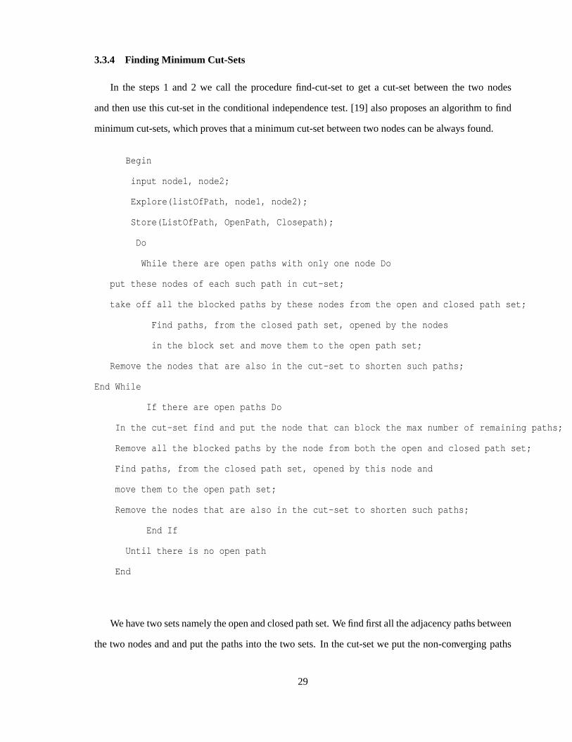
3.3.4 Finding Minimum Cut-Sets

In the steps1 and 2 we call the procedurefind-cut-setto get a cut-setbetweenthe two nodes

andthenusethis cut-setin theconditionalindependencetest.[19] alsoproposesanalgorithmto find

minimumcut-sets,whichprovesthataminimumcut-setbetweentwo nodescanbealwaysfound.

Begin

input node1, node2;

Explore(listOfPath, node1, node2);

Store(ListOfPath, OpenPath, Closepath);

Do

While there are open paths with only one node Do

put these nodes of each such path in cut-set;

take off all the blocked paths by these nodes from the open and closed path set;

Find paths, from the closed path set, opened by the nodes

in the block set and move them to the open path set;

Remove the nodes that are also in the cut-set to shorten such paths;

End While

If there are open paths Do

In the cut-set find and put the node that can block the max number of remaining paths;

Remove all the blocked paths by the node from both the open and closed path set;

Find paths, from the closed path set, opened by this node and

move them to the open path set;

Remove the nodes that are also in the cut-set to shorten such paths;

End If

Until there is no open path

End

Wehavetwo setsnamelytheopenandclosedpathset.Wefind first all theadjacency pathsbetween

thetwo nodesandandput thepathsinto thetwo sets.In thecut-setwe put thenon-converging paths

29

thatareconnectedto boththenodes.This is donebecausethesehave to bein every valid cut-set.This

is repeatedto find a nodethat canblock the maximumnumberof paths. Put this in the cut-setand

repeattill all theopenpathsareblocked.

3.3.5 Complexity Analysis

In general,most of the running time of learningalorithmsis consumedby dataretrieval from

databases.SupposeadatasethasN attributes,themaximumnumberof possiblevaluesof any attribute

is r, andan attribute hasa maximumof k parents.The computationof mutual informationrequires

at themostO�r2 � basicoperationsandcomputaionof conditionalmutualinformationrequiresat the

mostO�rk 2 � basicoperations,sincethe conditionsethask nodesat the most. So, the conditional

mutualinformationtesthasacomplexity of O�rN � . Thefirst stephasacomplexity of O

�N logN � steps,

for sortingthemutualinformationof pairs. TheprocedurehasO�N � basicoperations.Soasa whole

with respectto theCI tests,Step1 needsO�N2 � mutualinformationcomputationsandStep2 needsat

mostO�N2 � numberof CI tests.Similarly Step3 requiresat mostO

�N2 � numberof CI tests,because

adescisionrequiresoneCI test.SoasawholethealgorithmrequiresO�N2 � CI testsin theworstcase.

30

CHAPTER 4

SAMPLING

Bayesiannetworks arethe bestsuitedto representjoint probability distributions,asthey include

theconditionalindependencerelationshipsamongthevariablesin thenetwork. An attractive feature

of Bayesiannetwork is that its amenabilityto recursive andincrementalcomputationof schemes.Let

H denoteanhypothesis,en � e1 � e2 � �-�-� en denoteasequenceof dataobservedin thepast,andedenotea

new fact. Theoriginal way to calculatethebelief in H, P�H � en � e� would beto addthenew datae to

thepastdataen andperformaoverall computationof theeffectonH of theentiredataseten 1 � en � e.

Thiscomputationis timeandmemoryintensivebecausethecomputationof P�H � en � e� becomesmore

andmorecomplex asthesizeof thesetincreases.Thiscalculationcanbesimplifiedby discardingthe

pastdataoncewehavecomputedP�H � en � . Now wecancalculatethevalueof thenew databy Eq.4.1

P�H � en � e� � P

�H � en � P

�e � en � H �

P�e � en � (4.1)

Also, we know from Eq.3.2

P�H � e� � P

�e � H � P � H �

P�e� (4.2)

ComparingEq. 4.1 andEq. 4.2 we canseethat theold belief P�H � en � assumestherole of prior

probability in thecomputationof the new impact. It canalsobe seenthat it completelysummarizes

the pastexperiencesand if we needupdating,we needto multiply only by that likelihood function

P�e � en � H � , whichaswecanseegiventhehypothesisandpastobservationsit measurestheprobability

of the new datae. Likelihood is the hypotheticalprobability that an event that hasalreadyoccured

would yield a specificoutcome. The conceptdiffers from that of a probability in that a probability

refersto theoccurenceof futureevents,while a likelihoodrefersto pasteventswith known outcomes.

This recursive formulation still would be cumbersomebut for the fact that the likelihood function

31

is often independentof the pastdataandinvolvesonly e andH. Using the condtionalindependence

conditionwe canwrite,

P�e � en � H � � P

�e � H � and P

�e � en �/. H � � P

�e �0. H � (4.3)

anddividing Eq.4.1by thecomplementaryequationfor . H, wecanwrite

O�H � en 1 � � O

�H � en � L � e � H � (4.4)

If we multipy thecurrentposterioroddsO�H � en � by the likehoodratio of e, uponthe arrival of

eachnew datae, asshown in Eq. 4.4, shows a simplerecursive procedurefor updatingthe posterior

odds.Oddsis theprobabilitythattheevenwill occurdividedby theprobabilitythattheeventwill not

occur. O�H � en � is theprior oddsrelative to thenext observation,while O

�H � is theposterioroddsthat

hasevolvedfrom thepreviousobservationnot includedin en. Takingthelogarithmof Eq.4.4,

logO�H � en � � logO

�H � en � � logL

�e � H � (4.5)

Thesimplicity of the log-likelihoodcalculationhadled to a variety of applications,especiallyin

intelligencegatheringtasks.For eachnew report,we canestimatethelikelihoodratioL, whichcanbe

easilyincorporatedin thealreadyaccumulatedoverall belief in H.

4.1 CausalNetworks

The importantrequirementof Bayesiannetwork is that it incorporatesd-separationpropertiesof

thedomainmodeledandit neednot reflectcause-effect relations.But thereis, however, agoodreason

to strive for causalnetworks. Causationis one of the basicprimitives of probability becauseit is

an indispensibletool for structuringandspecifyingprobabilisticknowledge. Sincethe semanticsof

causalrelationshipsarepreservedby thesyntaxof probabilisticmanipulationsnoauxillarydevicesare

neededto force conclusions.For exampleif I figuredout that thecauseof my slippingwasdueto a

wet pavement,I could no longerconsiderothereventsasthe wetnessof the pavementis confirmed.

The factsthat it rainedthat day or the sprinklerwas on or my friend also slippedandbroke a leg

shouldno longerbeconsideredoncethewetnessof thepavementis identifiedasthedirectcauseof the

32

D

A B

D

A B

D

A B

(a)

(b) (c)

Figure4.1.CausalDiagram.

accident.Theasymmetryconveyedby thecausaldirectionalitycanbeusedfor encodingmorecomplex

andintricatepatternsof relationships.It cannow beunderstoodthatoncea consequenceis observed

its causescanno longerremainindependentbecauseconfirmingonecauselowers the likelihoodof

theother. Causaldirectionalityconveys themessagethat two eventsdo not becomerelevent to each

othermerelyby virtue of predictinga commonconsequence,but they do becomerelevant whenthe

consequenceis actually observed. The oppositeis true for two consequencesof a commoncause,

typically thetwo becomeindependentuponlearningthecause,asdiscussedwhenlearningthestructure

from data.

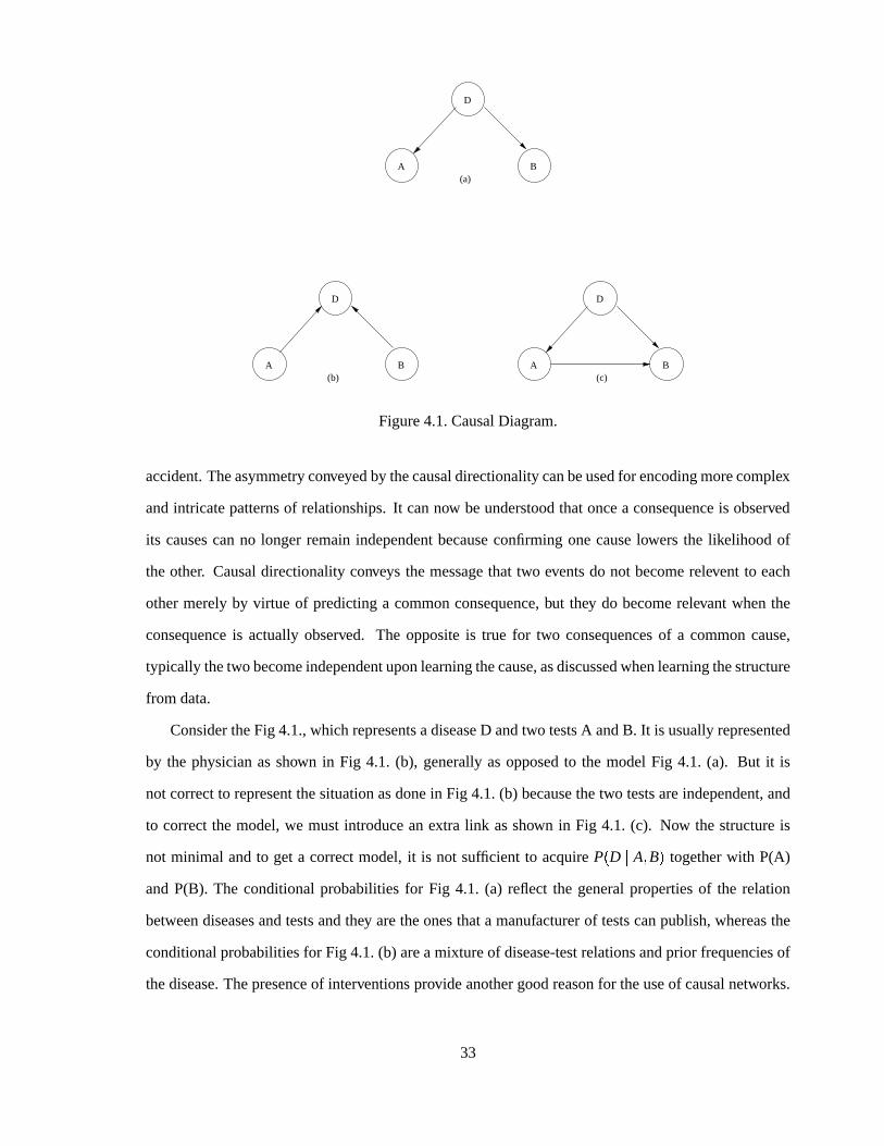
ConsidertheFig 4.1.,which representsadiseaseD andtwo testsA andB. It is usuallyrepresented

by the physicianasshown in Fig 4.1. (b), generallyasopposedto the modelFig 4.1. (a). But it is

not correctto representthesituationasdonein Fig 4.1.(b) becausethetwo testsareindependent,and

to correctthe model,we must introducean extra link asshown in Fig 4.1. (c). Now the structureis

not minimal andto get a correctmodel, it is not sufficient to acquireP�D � A � B� togetherwith P(A)

andP(B). The conditionalprobabilitiesfor Fig 4.1. (a) reflect the generalpropertiesof the relation

betweendiseasesandtestsandthey aretheonesthata manufacturerof testscanpublish,whereasthe

conditionalprobabilitiesfor Fig 4.1.(b) areamixtureof disease-testrelationsandprior frequenciesof

thedisease.Thepresenceof interventionsprovide anothergoodreasonfor theuseof causalnetworks.

33

7

96

5

4

83

2

1

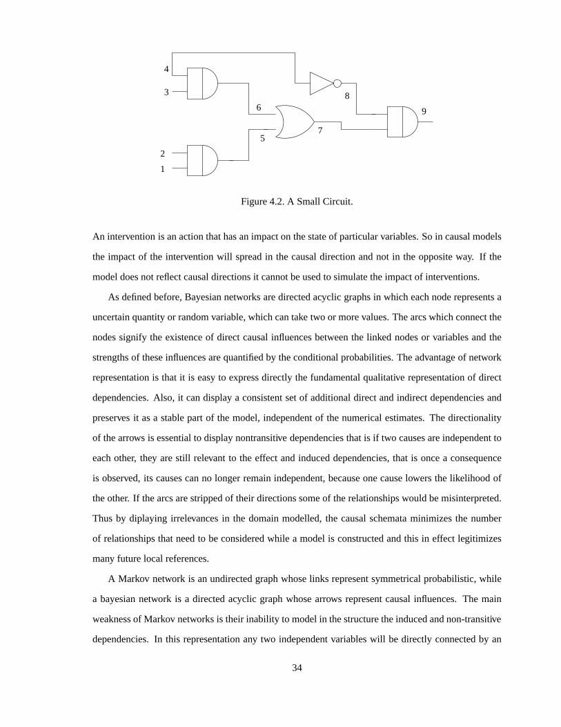
Figure4.2.A SmallCircuit.

An interventionis anactionthathasanimpacton thestateof particularvariables.Soin causalmodels

the impactof the interventionwill spreadin the causaldirectionandnot in the oppositeway. If the

modeldoesnot reflectcausaldirectionsit cannotbeusedto simulatetheimpactof interventions.

As definedbefore,Bayesiannetworksaredirectedacyclic graphsin which eachnoderepresentsa

uncertainquantityor randomvariable,whichcantake two or morevalues.Thearcswhichconnectthe

nodessignify the existenceof direct causalinfluencesbetweenthe linked nodesor variablesandthe

strengthsof theseinfluencesarequantifiedby theconditionalprobabilities.Theadvantageof network

representationis that it is easyto expressdirectly thefundamentalqualitative representationof direct

dependencies.Also, it candisplaya consistentsetof additionaldirectandindirectdependenciesand

preserves it asa stablepart of themodel,independentof thenumericalestimates.Thedirectionality

of thearrows is essentialto displaynontransitive dependenciesthatis if two causesareindependentto

eachother, they arestill relevant to the effect andinduceddependencies,that is oncea consequence

is observed, its causescanno longerremainindependent,becauseonecauselowersthe likelihoodof

theother. If thearcsarestrippedof their directionssomeof therelationshipswouldbemisinterpreted.

Thusby diplaying irrelevancesin the domainmodelled,the causalschemataminimizesthe number

of relationshipsthatneedto beconsideredwhile a modelis constructedandthis in effect legitimizes

many futurelocal references.

A Markov network is anundirectedgraphwhoselinks representsymmetricalprobabilistic,while

a bayesiannetwork is a directedacyclic graphwhosearrows representcausalinfluences.The main

weaknessof Markov networksis their inability to modelin thestructuretheinducedandnon-transitive

dependencies.In this representationany two independentvariableswill be directly connectedby an

34

X1

X

X X X

X

X

X

X7

6

9

8

432

5

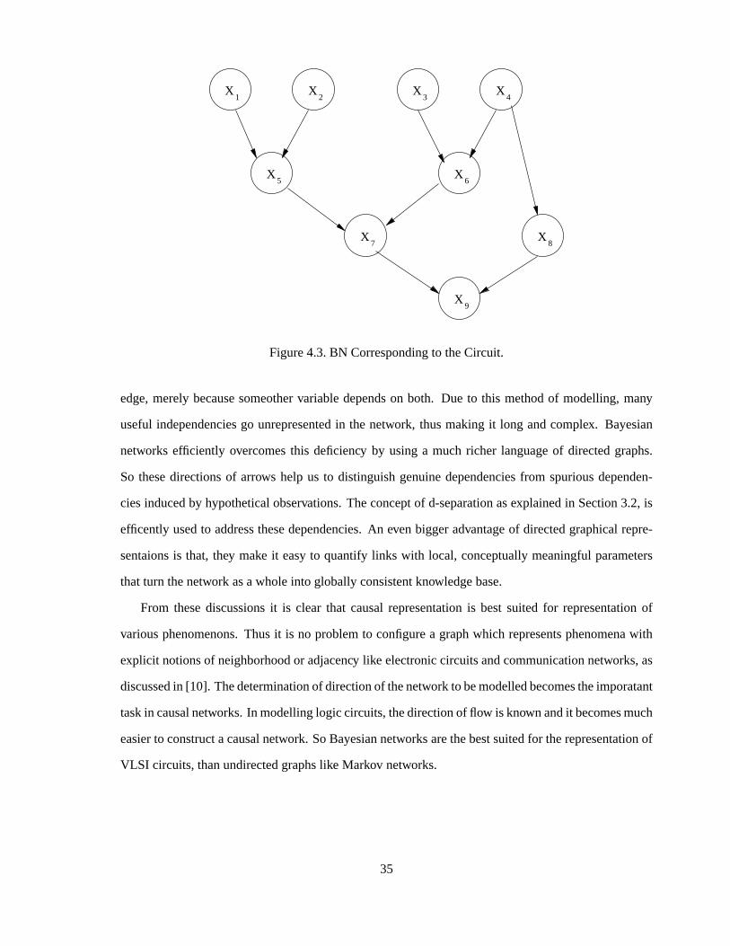
Figure4.3.BN Correspondingto theCircuit.

edge,merelybecausesomeothervariabledependson both. Due to this methodof modelling,many

useful independenciesgo unrepresentedin the network, thusmakingit long andcomplex. Bayesian

networks efficiently overcomesthis deficiency by usinga muchricher languageof directedgraphs.

So thesedirectionsof arrows help us to distinguishgenuinedependenciesfrom spuriousdependen-

ciesinducedby hypotheticalobservations.Theconceptof d-separationasexplainedin Section3.2, is

efficently usedto addressthesedependencies.An evenbiggeradvantageof directedgraphicalrepre-

sentaionsis that, they make it easyto quantify links with local, conceptuallymeaningfulparameters

thatturn thenetwork asawholeinto globally consistentknowledgebase.

From thesediscussionsit is clear that causalrepresentationis bestsuitedfor representationof

variousphenomenons.Thusit is no problemto configurea graphwhich representsphenomenawith

explicit notionsof neighborhoodor adjacency like electroniccircuitsandcommunicationnetworks,as

discussedin [10]. Thedeterminationof directionof thenetwork tobemodelledbecomestheimporatant

taskin causalnetworks. In modellinglogic circuits,thedirectionof flow is known andit becomesmuch

easierto constructacausalnetwork. SoBayesiannetworksarethebestsuitedfor therepresentationof

VLSI circuits,thanundirectedgraphslike Markov networks.

35

X1

X

X X X

X

X

X

X7

6

9

8

432

5

Figure4.4.Moral Graph.

4.2 Inference

The Bayesiannetwork not only modelscausalitybut alsomakesinferencemucheasier. The in-

ferencedonehereis split into many steps. First convert the network into a junction treeof cliques

andthenuseprobabilisticlogic samplingto acheive our purpose.Thestepsinvolve theformationof a

moralgraph,andtheprocessis calledcompilation,thenthemoralgraphis triangulated.Thecliqueset

is identifiedandthejunctiontreeof cliquesis formed.

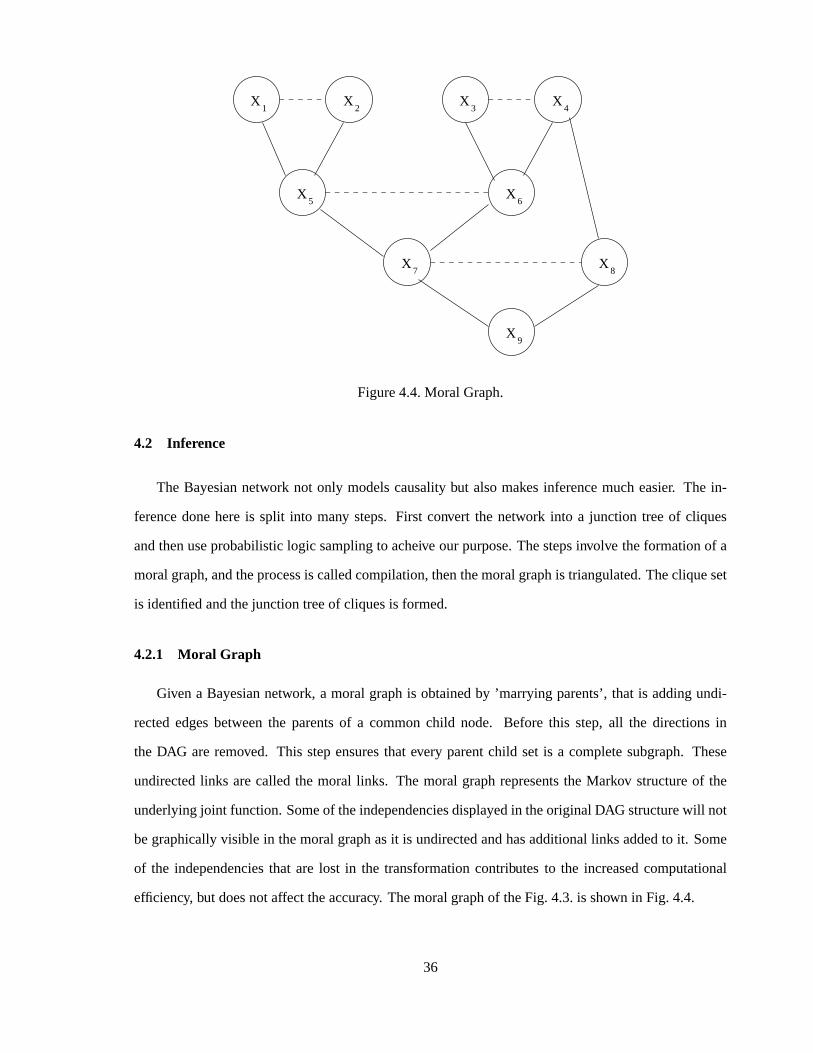
4.2.1 Moral Graph

Given a Bayesiannetwork, a moral graphis obtainedby ’marrying parents’,that is addingundi-

rectededgesbetweenthe parentsof a commonchild node. Before this step,all the directionsin

the DAG areremoved. This stepensuresthat every parentchild set is a completesubgraph.These

undirectedlinks arecalledthe moral links. The moral graphrepresentsthe Markov structureof the

underlyingjoint function.Someof theindependenciesdisplayedin theoriginalDAG structurewill not

begraphicallyvisible in themoralgraphasit is undirectedandhasadditionallinks addedto it. Some

of the independenciesthat are lost in the transformationcontributesto the increasedcomputational

efficiency, but doesnotaffect theaccuracy. Themoralgraphof theFig. 4.3.is shown in Fig. 4.4.

36

X1

X

X

X

X

X7

9

8

2

5

X X43

X6

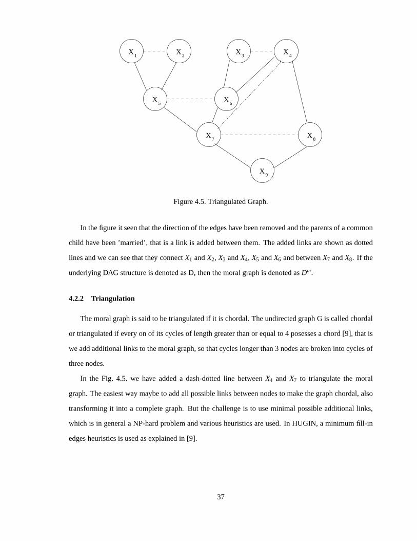
Figure4.5.TriangulatedGraph.

In thefigureit seenthatthedirectionof theedgeshavebeenremovedandtheparentsof acommon

child have been’married’, that is a link is addedbetweenthem. Theaddedlinks areshown asdotted

linesandwe canseethatthey connectX1 andX2, X3 andX4, X5 andX6 andbetweenX7 andX8. If the

underlyingDAG structureis denotedasD, thenthemoralgraphis denotedasDm.

4.2.2 Triangulation

Themoralgraphis saidto betriangulatedif it is chordal.TheundirectedgraphG is calledchordal

or triangulatedif every on of its cyclesof lengthgreaterthanor equalto 4 posessesa chord[9], thatis

weaddadditionallinks to themoralgraph,sothatcycleslongerthan3 nodesarebrokeninto cyclesof

threenodes.

In the Fig. 4.5. we have addeda dash-dottedline betweenX4 and X7 to triangulatethe moral

graph.Theeasiestwaymaybeto addall possiblelinks betweennodesto make thegraphchordal,also

transformingit into a completegraph. But the challengeis to useminimal possibleadditionallinks,

which is in generala NP-hardproblemandvariousheuristicsareused.In HUGIN, a minimumfill-in

edgesheuristicsis usedasexplainedin [9].

37

4 6 C = {X , X , X }

71 C = {X , X , X }

6 C = {X , X , X }

7C = {X , X , X }

7

C = {X , X , X } 7

C = {X , X , X } 7

5 3 4 6

2 7 4 8 3 5 4 1 2 5

6 7 8 9

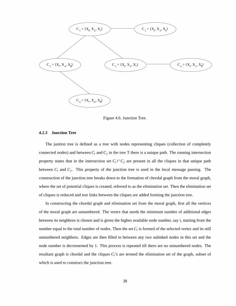
Figure4.6.JunctionTree.

4.2.3 Junction Tree

The juntion tree is definedas a tree with nodesrepresentingcliques(collection of completely

connectednodes)andbetweenCi andCj in thetreeT thereis a uniquepath.Therunningintersection

propertystatesthat in the intersectionsetCi � Cj are presentin all the cliquesin that uniquepath

betweenCi andCj . This propertyof the junction tree is usedin the local messagepassing. The

constructionof thejunctiontreebreaksdown to theformationof chordalgraphfrom themoralgraph,

wherethesetof potentialcliquesis created,referredto astheeliminationset.Thentheeliminationset

of cliquesis reducedandtreelinks betweenthecliquesareaddedforming thejunctiontree.

In constructingthe chordalgraphandeliminationset from the moral graph,first all the vertices

of themoralgraphareunnumbered.Thevertex thatneedstheminimumnumberof additionaledges

betweenits neighborsis chosenandis giventhehighesavailablenodenumber, sayi, startingfrom the

numberequalto thetotalnumberof nodes.ThenthesetCi is formedof theselectedvertex andits still

unnumberedneighbors.Edgesarethenfilled in betweenany two unlinked nodesin this setandthe

nodenumberis decrementedby 1. This processis repeatedtill thereareno unnumberednodes.The

resultantgraphis chordalandthe cliquesCi ’s aretermedthe eliminationsetof the graph,subsetof

which is usedto constructthejunctiontree.

38

In ourexamplemoralgraph,nodeX9 is first selectedsincenofill-in edgeis neededbecauseall the

neighbors(rememberthemoralgraphis undirected)arealreadylinked. This nodeX9 is assignedthe

number9 - the total numberof nodesin thegraph. ThesetC9 is thenformedby nodes� X9 � X8 � X7 � .ThenodesX8 andX7 arenot yet numbered.For thesecondcycle, thenodesX8 � X7 � X6 � andX4 cannot

beselectedasthey eachwould requireonefill-in edgesamongstits neighbors,whereastheneighbors

of X3 doesnot requireany fill-in edges.HenceX3 is numbered8 in our exampleandC8 is formedby

� X3 � X4 � X6 � . For thethird cycle, we thenselectX2, numberingit as7 andformingC7 �1� X2 � X1 � X5 � .In thefourthcycle,nodeX1 is assigned6 andC6 �2� X1 � is formed.WethenselectX5, assignanumber

5, andformC5 �3� X5 � X6 � X7 � . NodeX8 is assignednumber4, andC4 �3� X8 � X7 � X4 � is formed.In this

step,afill-in edgebetweenX4 andX7 is added.Wethenassignthenumber3 to X7, thenumber2 to X6,

andthenumber1 to X4.

Theresultanteliminationset � Ci � (whichis thesupersetof theclique-set)obtainedfromtherunning

exampleare

� C9 �� C1 � � �4� X9 � X8 � X7 �5�6� X3 � X4 � X6 �5�6� X2 � X1 � X5 �5�6� X1 �5�6� X5 � X6 � X7 �5�� X8 � X7 � X4 �5�6� X7 � X6 � X4 �5�6� X6 �5�6� X4 �4�

For eachcliqueCi of theCliquesetorderedto have runningintersectionproperty, wehave to adda

link to cliqueCj where j is anyone of theset � 1 � 2 ��7� i � 1 � suchthatCi � � C1 & C2 & �� & Ci 1 ��8 Cj

Figure4.6. shows the junction tree for the exampleconsidered.It canbe observed that the cliques

in our exampleareC1 �9� X4 � X6 � X7 � , C2 �9� X7 � X4 � X8 � , C3 �9� X5 � X6 � X7 � , C4 �9� X1 � X2 � X5 � , C5 �� X3 � X4 � X6 � , andC6 �%� X7 � X8 � X9 � . This cliquesareobtainedby reducingtheeliminationset.For our

examplein Figure4.6.,for thecliqueC6, wehaveto find thesetthatcontainsthefollowing intersection

set

C6 � � C1 & C2 & �� & C6 � � �4� X7 � X8 � X9 � � � X4 � X6 � X7 � X8 � X5 � X1 � X2 � X3 �4�� X7 � X8 �

It is obvious that � X7 � X8 � 8 C2, hencewe adda link betweenC6 andC2. Theseparatorsetis the

non-nullsetof nodescommonbetweenevery cliquewith anedgebetweenthem.Theseseparatorsets

areusedfor evidencepropagation.If thereweretwo cliquesthatarenotconnectedby anedgeandstill

39

have commonvariablesthenthesevariablesmustbe presentin all thecliquesin betweentheunique

pathbetweenthe two cliquesto guaranteecorrectprobability valuesfor the randomvariablesof the

entirenetwork while probabilitiesareupdatedby local propagation.As it canbeseenthatC3 andC6

bothcontainX7 andX7 is alsopresentin all thecliquesin thepathfrom C3 to C6 namelyin C1 andC2.

This helpsto preserve probabilitiesof the randomvariablesof the entirenetwork while updatingan

evidenceby local messagepassing.

4.2.4 Propagationin Junction Trees

After the junction treeof cliquesis formed, the next stepis to form the distribution function of

cliques.It hasbeenprovedin [9] thatthedependency propertiesof a DAG, which carryover to moral

graphs,arealsopreserved in the triangulatedmoral graph. Also, the joint probability function that

factorizeson the moral graphwill alsodo so on the triangulatedon sinceeachclique in the moral

graphis eithera clique in this graphor a subsetof a clique. Let � xc � be thesetof nodesin cliquec

in the junction tree. The joint probability functionover thesevariablesis denotedby p�xc � . Let � xs �

bethesetof nodesin a separatorsets betweentwo cliquesin the junction tree. Thejoint probability

functionover thesevariablesis denotedby p�xs � . Let CSdenotethesetof all cliquesandSSdenote

thesetof separatorsbetweentheadjacentcliquesin the junction tree. The joint probability function

factorizesover thejunctiontreein thefollowing form [9]:

p�x1 �� xN � � ∏

c: CSp�xc ��; ∏

s: SSp�xs � (4.6)

A separatorsets is containedin two neighboringcliques,c1 andc2. If we associateeachof the

producttermsover the separatorsin the denominatorwith one its two neighboringcliques,say c1,

then we canwrite the joint probability function in a pureproductform as follows. Let φc1

�xc1 � �

p�xc1 ��; p

�xs � andφc2

�xc2 � � p

�xc2 � , thenthejoint probabilityfunctionasexpressedas:

P�x1 �� xN � � ∏

c: CSφc�xc � (4.7)

40

A A, φ φ B,

Bφ S,

S

Figure4.7.Two Cliqueswith theSeparatorSet.

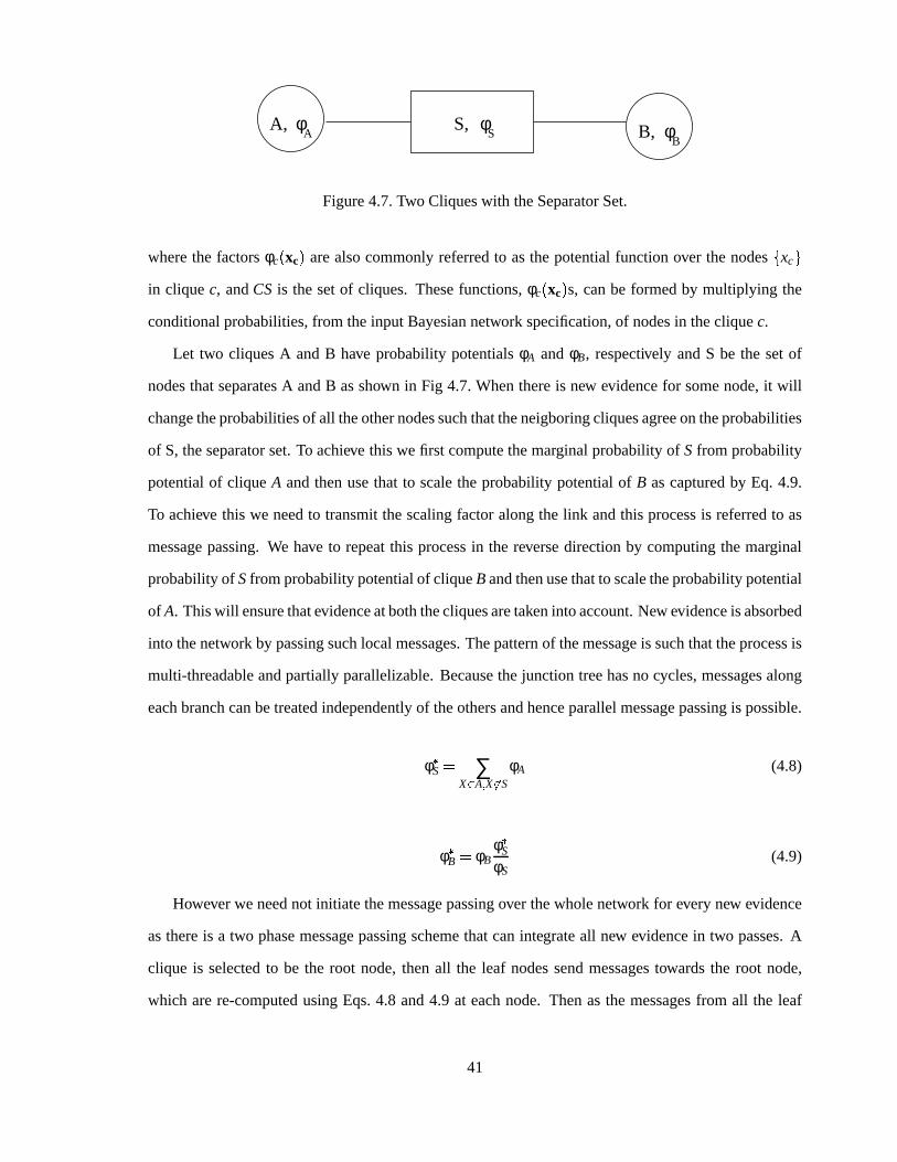
wherethe factorsφc�xc � arealsocommonlyreferredto asthepotentialfunctionover thenodes� xc �

in cliquec, andCS is thesetof cliques. Thesefunctions,φc�xc � s, canbe formedby multiplying the

conditionalprobabilities,from theinput Bayesiannetwork specification,of nodesin thecliquec.

Let two cliquesA andB have probability potentialsφA andφB, respectively andS be the setof

nodesthatseparatesA andB asshown in Fig 4.7.Whenthereis new evidencefor somenode,it will

changetheprobabilitiesof all theothernodessuchthattheneigboringcliquesagreeontheprobabilities

of S, theseparatorset.To achieve this we first computethemarginal probabilityof S from probability

potentialof clique A andthenusethat to scalethe probability potentialof B ascapturedby Eq. 4.9.

To achieve this we needto transmitthescalingfactoralongthe link andthis processis referredto as

messagepassing.We have to repeatthis processin the reversedirectionby computingthemarginal

probabilityof Sfrom probabilitypotentialof cliqueB andthenusethatto scaletheprobabilitypotential

of A. Thiswill ensurethatevidenceatboththecliquesaretakenintoaccount.New evidenceisabsorbed

into thenetwork by passingsuchlocalmessages.Thepatternof themessageis suchthattheprocessis

multi-threadableandpartially parallelizable.Becausethejunction treehasno cycles,messagesalong

eachbranchcanbetreatedindependentlyof theothersandhenceparallelmessagepassingis possible.

φ <S � ∑X : A � X =: S

φA (4.8)

φ <B � φBφ <SφS

(4.9)

Howeverwe neednot initiate themessagepassingover thewholenetwork for every new evidence

asthereis a two phasemessagepassingschemethatcanintegrateall new evidencein two passes.A

clique is selectedto be the root node,thenall the leaf nodessendmessagestowardsthe root node,

which arere-computedusingEqs.4.8 and4.9 at eachnode. Thenasthe messagesfrom all the leaf

41

nodesarereceived,they arepassedbackfrom therootcliquetowardstheleaves.Notethatthisensures

that alongany onelink, we have messagesalongboth directions,thus,ensuringall nodeshave been

updatedbasedon informationfrom all thenew evidence.

4.2.5 Probabilistic Logic Sampling

ProbabilisticLogic Samplingis a methodproposedby Henrion[56] which employs a stochastic

simulationapproachto make probabilistic inferencesin large multiply connectednetworks. If we

representa Bayesiannetwork by a sampleof m deterministicscenarioss=1,2,.....mandLs�x� is the

truthof eventx in scenarios, thenuncertaintyaboutx canberepresentedby a logic sample,thatis the

thevectorof truthvaluesfor thesampleof scenarios:

Lx >@? L1�x� � L2

�x� � �-�-� Lm

�x�BA � (4.10)

If we have the prior probability px, we canusea randomnumbergeneratorto producea logic

samplefor x. This methodof samplingproceedsasexplainedbelow, given a Bayesiannetwork with

priorsspecifiedfor all sourcevariablesandconditionaldistributionsfor all others:

1. Usea randomnumbergeneratorto producea samplevaluefor eachroot nodein the network

and a sampleimplication rule for eachparameterof eachconditionaldistribution, using the

correspondingprobabilities.

2. Proceeddown throughthe network following the directionof the arrows from the root nodes

using simple logical operationsto obtain the truth of eachvariable from its parentsand the

implicationrules.

3. Repeatsteps2 and3 m timesto obtaina logic samplefor eachvariable.

4. Estimateprior marginal probability of any event by computingthe numberof times in which

they aretrue.

5. Estimateposteriorprobability on any of the alreadycomputedvariableas the fraction of the

numberof timestheeventoccursout of thepossiblescenariosin which thegiven conditionis

true.

42

We stopwith step3 aswe needonly the logic sampleandwe do not computetheposteriorprob-

abilites. We usethis logic samplingmethodinsideeachcliqueof the junction tree. To startwith, the

first clique is consideredandthesamplingis doneinsideto arrive at thesamplesfor thenodesinside

theclique. Oncevaluesarefixedfor thesenodes,they arepropagatedto thenext cliquewith thehelp

of theseparatorset.As thenodesof theseparatorsetarein boththecliques,oneor moreof thenodes

areinstantiated.With thesevaluestherestof thenodesaresampledwith logic samplingandthisgoes

on till theendof thejunctiontree.

43

CHAPTER 5

EXPERIMENT AL RESULTS

This model proves to be an efficient techniquefor power estimationby providing a minimum

numberof samples.As saidbeforethemethodbridgesthegapbetweensimulative andprobabilistic

techniques.This is acheivedby aneffecientmodelof Bayesiannetwork, by learningthestructurefrom

theinput data.Thelearnedstructureof theBayesiannetwork representsthegraphicalstructureof the

inputdata.Thelearnedstructurecannow beusedto generateany numberof vectors.Thegenerationof

thevectorsetis doneefficiently by exploiting thesamplingtechniquesappliedon Bayesiannetworks.

Samplingis doneto derive vectorsin any neededcompactionratio. Thereducedvectorsetis thenfed

into HSPICEto getanaccurateestimateof theaveragepower. Thepower estimateis thencompared

with the valuegot from simulatingthe large vectorset. If a is the original lengthof the vectorand

b is thecompactedlength,thena; b is calledthecompactionratio (CR). We have acheived very high

compactionratiosof upto300whichhave never beenacheivedbefore.

We have fixed the larger vector set to be 60,000highly-correlatedinput patternsgeneratedby

simulatingthe variousbenchmarkcircuits. The vectorswere thentaken from randomoutputnodes

of thesecircuits. This is doneto inducea high correlationbetweenthe vectorsso that they areas

closeaspossibleto the real world data. Also differentbenchmarkcircuits wereusedfor generating

thesevectors,for exampleto obtainvectorsfor C499thecircuit C3540wassimulated.Thecorrelation

betweenthevectorscanbeseenin theconstructedBayesiannetwork.

Theoverall processflow is asshown in Fig. 5.1.. As shown, we first generatethethelargevector

set.Thenthepowerconsumedby eachbenchmarkcircuit is calculatedusingthelargevectorsetasthe

input stimuli. This valueis usedasthebasisfor comparisonwith thepower estimategeneratedfrom

thecompactedvectorset.

Thenthesecondstepis tousethisvectorsetto learntheBayesiannetwork. WeusePowerConstruc-

tor [16] to acheive our purpose.Thepower constructoris anefficient tool which providesanaccurate

44

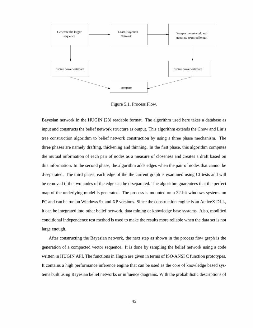
Generate the larger sequence

Learn Bayesian Network

Sample the network andgenerate required length

hspice power estimatehspice power estimate

compare

Figure5.1.ProcessFlow.

Bayesiannetwork in the HUGIN [23] readableformat. The algorithmusedheretakesa databaseas

inputandconstructsthebeliefnetwork structureasoutput.ThisalgorithmextendstheChow andLiu’s

treeconstructionalgorithmto belief network constructionby using a threephasemechanism.The

threephasesarenamelydrafting,thickeningandthinning. In thefirst phase,this algorithmcomputes

the mutualinformationof eachpair of nodesasa measureof closenessandcreatesa draft basedon

this information.In thesecondphase,thealgorithmaddsedgeswhenthepair of nodesthatcannotbe

d-separated.The third phase,eachedgeof the thecurrentgraphis examinedusingCI testsandwill

beremovedif thetwo nodesof theedgecanbed-separated.Thealgorithmguarenteesthattheperfect

mapof theunderlyingmodelis generated.Theprocessis mountedon a 32-bit windows systemson

PCandcanberunonWindows 9x andXP versions.Sincetheconstructionengineis anActiveX DLL,

it canbeintegratedinto otherbelief network, datamining or knowledgebasesystems.Also, modified

conditionalindependencetestmethodis usedto make theresultsmorereliablewhenthedatasetis not

largeenough.

After constructingtheBayesiannetwork, the next stepasshown in theprocessflow graphis the

generationof a compactedvectorsequence.It is doneby samplingthe belief network usinga code

written in HUGIN API. Thefunctionsin Huginaregivenin termsof ISO/ANSIC functionprototypes.

It containsa high performanceinferenceenginethatcanbeusedasthecoreof knowledgebasedsys-

temsbuilt usingBayesianbeliefnetworksor influencediagrams.With theprobabilisticdescriptionsof

45

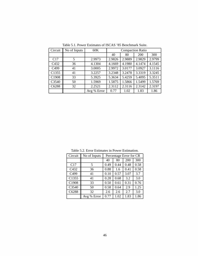
Table5.1.PowerEstimatesof ISCAS’85 BenchmarkSuite.

Circuit No of Inputs 60K CompactionRatio40 80 200 300

C17 5 2.9973 2.9826 2.9889 2.9829 2.9799C432 36 4.1304 4.1669 4.1980 4.1474 4.1545C499 41 3.0005 2.9972 3.0177 3.0927 3.1116C1355 41 3.2257 3.2348 3.2478 3.3319 3.3245C1908 33 5.3925 5.3634 5.4259 5.4095 5.3511C3540 50 1.5969 1.5875 1.5866 1.5499 1.5769C6288 32 2.2521 2.3112 2.3116 2.3142 2.3197

Avg % Error 0.77 1.02 1.83 1.86

Table5.2.ErrorEstimatesin PowerEstimation.

Circuit No of Inputs PercentageError for CR40 80 200 300

C17 5 0.49 0.44 0.48 0.58C432 36 0.88 1.6 0.41 0.58C499 41 0.10 0.57 3.07 3.7C1355 41 0.28 0.68 3.2 3.0C1908 33 0.50 0.61 0.31 0.76C3540 50 0.58 0.64 2.9 1.25C6288 32 2.6 2.6 2.7 3.0

Avg % Error 0.77 1.02 1.83 1.86

46

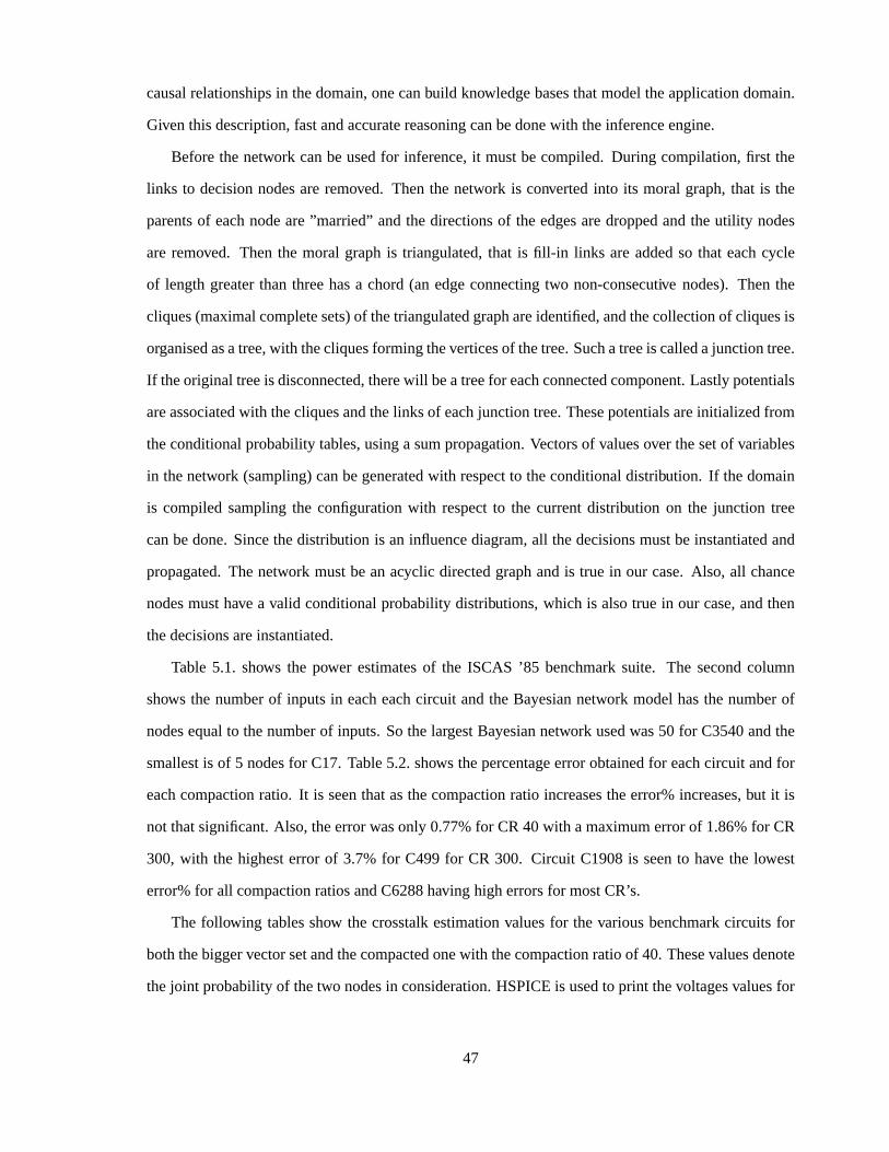
causalrelationshipsin thedomain,onecanbuild knowledgebasesthatmodeltheapplicationdomain.

Giventhisdescription,fastandaccuratereasoningcanbedonewith theinferenceengine.

Beforethenetwork canbeusedfor inference,it mustbecompiled. During compilation,first the

links to decisionnodesareremoved. Thenthe network is convertedinto its moral graph,that is the

parentsof eachnodeare”married” andthedirectionsof theedgesaredroppedandtheutility nodes

areremoved. Thenthe moral graphis triangulated,that is fill-in links areaddedso that eachcycle

of lengthgreaterthanthreehasa chord(an edgeconnectingtwo non-consecutive nodes). Thenthe

cliques(maximalcompletesets)of thetriangulatedgraphareidentified,andthecollectionof cliquesis

organisedasatree,with thecliquesformingtheverticesof thetree.Suchatreeis calledajunctiontree.

If theoriginal treeis disconnected,therewill beatreefor eachconnectedcomponent.Lastlypotentials

areassociatedwith thecliquesandthelinks of eachjunctiontree.Thesepotentialsareinitialized from

theconditionalprobabilitytables,usinga sumpropagation.Vectorsof valuesover thesetof variables

in thenetwork (sampling)canbegeneratedwith respectto theconditionaldistribution. If thedomain

is compiledsamplingthe configurationwith respectto the currentdistribution on the junction tree

canbedone.Sincethedistribution is an influencediagram,all thedecisionsmustbeinstantiatedand

propagated.Thenetwork mustbean acyclic directedgraphandis true in our case.Also, all chance

nodesmusthave a valid conditionalprobabilitydistributions,which is alsotrue in our case,andthen

thedecisionsareinstantiated.

Table 5.1. shows the power estimatesof the ISCAS ’85 benchmarksuite. The secondcolumn

shows the numberof inputsin eacheachcircuit andtheBayesiannetwork modelhasthenumberof

nodesequalto thenumberof inputs.SothelargestBayesiannetwork usedwas50 for C3540andthe

smallestis of 5 nodesfor C17. Table5.2.shows thepercentageerrorobtainedfor eachcircuit andfor

eachcompactionratio. It is seenthatasthecompactionratio increasestheerror%increases,but it is

not thatsignificant.Also, theerrorwasonly 0.77%for CR 40 with amaximumerrorof 1.86%for CR

300, with the highesterror of 3.7%for C499for CR 300. Circuit C1908is seento have the lowest

error%for all compactionratiosandC6288having higherrorsfor mostCR’s.

The following tablesshow the crosstalkestimationvaluesfor the variousbenchmarkcircuits for

boththebiggervectorsetandthecompactedonewith thecompactionratioof 40. Thesevaluesdenote

thejoint probabilityof thetwo nodesin consideration.HSPICEis usedto print thevoltagesvaluesfor

47

Table5.3.JointProbabilitySwitchingEstimatefor Nodes300and330of C432for 60K.

Node300 Node330State 00 01 10 1100 0.06 0.19 0.19 0.5401 0 0 0 010 0 0 0 011 0 0 0 0

Table5.4.JointProbabilitySwitchingEstimatefor Nodes300and330of C432for CR 40.

Node300 Node330State 00 01 10 1100 0.053 0.19 0.19 0.5601 0 0 0 010 0 0 0 011 0 0 0 0

theparticularinput vectorsof thetwo nodes,which arethenchangedto their switchingvalues.From

thesevoltagevaluesthejoint probability is calculatedby finding thenumberof occurences.Themain

ideaof thispartof theresultis to estimatetheworst-casecrosstalk,but thetablealsogivesanestimate

of theprobabilityof leakageoccuringin thenodes.We have limited to only a few nodesdueto high

runningtime takenby HSPICE,otherwiseany numberor all of thenodescanbeestimated.

The tables5.3. and5.4. wereplotted for the nodes300 and330 which are the inputs to a gate

selectedat random.The table5.4.shows that the compactedvectorsetgave the similar crosstalkes-

timation resultsas the original vectorsetusedin 5.3., proving that the smallervectorset is equally

efficient in modellingcrosstalk.Thesimultaneousswitchingnoiseof onenodeswitchingfrom 0 to 1

andtheotherswitching1 to 0 at thesametimeyieldsthemaximumcrosstalk.Herewecanseethatthe

particularsetof input usedhaszeroor very low worstcaseswitchingnoise.Also we canseethat the

leakageis prettyhigh,andsothedesignersshouldpaymoreattentionto reducingtheleakage.

Thetwo tables5.5.and5.6.arefor thecircuit C499,consideringthenodes557and558.Wecansee

heretoo that thecompactedvectorsetyieldedsimilar valueswith respectto theresultfrom thelarger

vectorset. For this setof inputs the couplingnoiseis assignificantasthe leakage.The worst-case

crosstalkprobabilityis .07for node557switchingfrom 0 to 1 andnode558switchingfrom 1 to 0 and

.07for 557switchingfrom 1 to 0 and558switchingfrom 0 to 1.

48


Node557 Node558State 00 01 10 1100 0.054 0.058 0.059 0.05701 0.066 0.06 0.07 0.06610 0.06 0.071 0.063 0.06511 0.065 0.062 0.068 0.07


Node557 Node558State 00 01 10 1100 0.056 0.057 0.059 0.05701 0.064 0.06 0.07 0.06410 0.06 0.07 0.063 0.06711 0.066 0.06 0.068 0.07


Node141 Node113State 00 01 10 1100 0.25 0 0 001 0 0.24 0 010 0 0 0.25 011 0 0 0 0.24


Node141 Node113State 00 01 10 1100 0.25 0 0 001 0 0.24 0 010 0 0 0.25 011 0 0 0 0.24

49


Node2427 Node2340State 00 01 10 1100 0.19 0.02 0.02 001 0.05 0.17 0 0.0210 0.05 0 0.16 0.0211 0.01 0.04 0.04 0.14


Node2427 Node2340State 00 01 10 1100 0.19 0.02 0.02 001 0.06 0.2 0 0.0210 0.06 0 0.16 0.0211 0.01 0.04 0.04 0.15

The tables5.7. and5.8. representsthe joint probablitydistribution of nodes141 and113 which

arethe two inputsof a NAND gate. Theparticularinput setshows that thereis a high probabilityof

leakagewhenboththenodesareswitchingfrom 0 to 0 andfrom 1 to 1.

Thetables5.9.and5.10.capturesthenodes2427and2340which areinputsof a NOR gate.Here

we canseea high probabilityof leakagethancrosstalknoiseasbothnodesswitchingfrom 0 to 0 and

1 to 1 have ahigh joint probability.

The nodesconsideredare4899and4925in the tables5.11.and5.12.. Herewe canseethat the

switchingfrom 1 to 1 in boththenodeshasthehighestprobability, showing highprobabilityof leakage.


Node4899 Node4925State 00 01 10 1100 0 0 0 0.0901 0 0 0 0.2110 0 0 0 0.2111 0 0 0 0.48

50


Node4899 Node4925State 00 01 10 1100 0 0 0 0.0901 0 0 0 0.2110 0 0 0 0.2111 0 0 0 0.48

51

CHAPTER 6

CONCLUSION

Herewe areableto modela framework for learninginput modelsandusethemto estimatepower

andcrosstalk.Thoughlot of researchwork hasbeendonein bothsimulativenadprobabilisticmethods,

they remainas two seperateentities. This work serves as a bridge effectively connectingthe two

methods.Thetechniqueproposedis uniqueandeffectively modelsthespatialcorrelationandfirstorder

temporalcorrelationbetweentheinputs.Also usingBayesiannetworkswearealsoableto includethe

causalitybetweenthenodeswhichcannotbemodelledusingundirectedgrpahslikeMarkov networks.

Amongthemajoradvantagesof thismethodaretheexcellentscalabilityto largecircuitsandtheability

to modelinput dependenciesusingtheconceptof tree-dependentBayesianNetworks.

1. We presenta unified graphbasedprobabilisticframework for power estimationthat takes into

accounthighorderspatialandfirst ordertemporaldependenciesthatarepresentin theinputs.

2. Modeling temporalcorrelationat the input nodesis automaticin way we setup the statesof

the randomvariablesof the BN. For spatialcorrelationamongthe input nodes,we learn an

approximatetree-dependentdistributionsin theprimaryinputsbasedon theinput statistics.

3. Theeasewith whichtheBayesiannetwork is built consideringthetimetakenmakestheapproach

highly favorableover building Markov networks,asconstructingthe latter is bothmemoryand

time intensive.

4. We alsotried othersamplingmethodsusingMatlabfrom BayesNet Toolboxfor matlab(BNT),

anopensourcesoftwareby Kevin Murphy [54] andalsotheopensourceProbabilisticNetwork

Library(PNL) from Intel [55], which is a C++ versionof theBayesNet toolbox for matlabby

Kevin Murphy. But neitherof themsuitedourpurposeandsoHugin [23] wasused.

52

5. Samplingthe Bayesiannetwork can also be doneusing Geniewith any one of the approxi-

mateinferencemethods.Theresultsobtainedweresimilar andit canbeusedto samplea large

Bayesiannetwork.

6. Experimentalresultsshow thatthemethodproposedby thisthesisis highly efficientandeffective

in variouswaysnamelythevery lesstime takento constructtheinput modelandalsosampling

it, not to forgetthevery low errorpercentageandhigh compactionratios.

Our future directionwould be integartingthis methodwith a vectorlessapproach.We intendto

usethis unified framework also with sequentialcircuits. Also, the presentwork modelsonly first

ordertemporalcorrelation.DynamicBayesiannetworksmustbeusedto acheive higerordertemporal

correlation.

53

REFERENCES

[1] S. Bhanja,N. Ranganathan,”Switching Activity Estimationof VLSI circuits using BayesianNetworks”, IEEE Trans.on VLSISystems, 2003.

[2] C. Tsui,R. Marculescu,D. Marculescu,M. Pedram,”Improving theefficiency of power simula-torsby inputvectorcompaction”,33rd DesignAutomationConference, pp.165-168,June1996.

[3] D. Marculescu,R. Marculescu,M. Pedram,”StochasticSequentialMachinesSynthesiswith Ap-plication to ConstrainedSequenceGenereation”, Proc. ACM/IEEEDesignAutomationConfer-ence, pp.696-701,June1996.

[4] D. Marculescu,R. Marculescu,M. Pedram,”StochasticSequentialMachinesSynthesiswith Ap-plication to ConstrainedSequenceGenereation”, ACM Trans.on DesignAutomationof Elec-tronic Systems, Vol.5,No.2,Jan2000.

[5] R. Marculescu,D. Marculescu,M. Pedram,”VectorCompactionusingDynamicMarkov Mod-els”, TechnicalReportCENG96-14,Univ. of SouthernCalifornia, Feb. 1996

[6] R. Marculescu,D. Marculescu,M. Pedram,”HierarchicalSequenceCompactionfor PowerEsti-mation”, Proc.ACM/IEEEDesignAutomationConference, Jun.1997.

[7] R. Marculescu,D. Marculescu,M. Pedram,”Adaptive Models for Input DataCompactionforPower Simulators”,Proc. ACM Asia and South-Pacific DesignAutomationConference, Japan,Jan.1997.

[8] R. Radjassamy, J.D. Carothers”VectorCompactionfor Efficient Simulation-BasedPower Esti-mation”, IEEE Symposiumon IC/Package DesignIntegration, pp.138-142,Feb1998.

[9] R.G.Cowell, A. P. David, S.L. Lauritzen,D. J.Spiegelhalter, “ProbabilisticNetworksandExpertSystems”,Springer-Verlag New York, Inc., 1999.

[10] J.Pearl,“ProbabilisticReasoningin IntelligentSystems:Network of PlausibleInference”, Mor-ganKaufmannPublishers,Inc., 1988.

[11] R. E. Neapolitan,”LearningBayesianNetworks”, PrenticeHall Seriesin Artificial Intelligence,2004.

[12] C. Hsu, W. Shen,“Vector Compactionfor Power Estimationwith Groupingand ConsecutiveSamplingTechniques”,IEEE International Symposiumon Circiuts and Systems, pp. 472-475vol.2, May 2002.

[13] A. Ghosh,S. Devadas,K. Keutzer, andJ. White, “Estimationof AverageSwitchingActivity inCombinationalandSequentialCircuits”, 29thDesignAutomationConference, pp.253-259,June1992.

54

[14] B. Ayari, B. Kaminska,“A New DynamicTestVectorCompactionfor AutomaticTestPatternGeneration”,IEEE Transactionson Computer-AidedDesignof IntegratedCircuitsandSystems,pp.353-358,March1994.

[15] T.J.Lambert,K. Saluja,”Methodsfor DynamicTestVectorCompactionin SequentialTestGen-eration”,Ninth InternationalConferenceon VLSIdesign, pp.166-169,Jan.1996.

[16] J. Cheng,D. Bell, W. Liu, ” LearningBayesianNetworks from Data: An Efficient ApproachBasedon InformationTheory”, Technical Report,Departmentof ComputerScience, Universityof Alberta, 1998.

[17] J.Cheng,D. Bell. W. Liu, ”LearningBelief Networksfrom Data:An InformationTheoryBasedApproach”,Proceedingsof theSixthACM InternationalConferenceon InformationandKnowl-edge Management, 1997.

[18] P. Spirtes,C. Glymour, R. Scheines,”Causation,PredictionandSearch”,2ndEdition,MIT Press,2000.

[19] S.Acid, L. M. Campos,”An algorithmfor findingminimumd-seperatingsetsin beliefnetworks”,Proceedingsof thetwelfthConferenceof Uncertaintyin Artificial Intelligence, 1996.

[20] R. Burch, F. N. Najm, andT. Trick, “A Monte Carlo Approachfor Power Estimation”, IEEETransactionson VLSISystems, vol.1-1,pp.63-71,March1993.

[21] R. Marculescu,D. Marculescu,M. Pedram,“Probabilistic Modeling of DependenciesDuringSwitchingActivity Analysis”, IEEE Transactionon Computer-AidedDesignof IntegratedCir-cuitsandSystems, vol. 17-2,pp.73-83,February1998.

[22] D.Heckerman,D. Geiger, andD. Chickering,“Learningbayesiannetworks: Thecombinationofknowledgeandstatisticaldata,” Tech. Rep.MSR-TR-94-09,MicrosoftResearch, 1994.

[23] URL http://www.hugin.com/

[24] C.Ababei,R.Marculescu,V. Sundarajan,“ProbabilisticAspectsof CrosstalkProblemsin CMOSICs”, Proc. IEEE CustomIntegratedCircuitsConf., May 2000.

[25] K. T. Tang,E. G. Friedman,“Estimationof On-ChipSimultaneousSwitchingNoiseon SignalDelayin SynchronousCMOSICs”, to befound...

[26] V. Tiwari, D. Singh, S. Rajagopal,G. Mehta, R. Patel, F. Baez, “ReducingPower in High-performanceMicroprocessors”,Proc. ACM/IEEEDesignAutomationConference, pp. 732-737,1998.

[27] L. Benini,M. Favalli, P. Olivo, B. Ricco,“A Novel Approachto Cost-effective Estimateof PowerDissipationin CMOSICs”, EuropeanDesignAutomationConference, pp.354-360,1993.

[28] S. M. Kang,“AccurateSimulationof Power Dissipationin VLSI Circuits”, Proc. IEEE Journalof SolidStateCircuits, vol. SC-21,no.5, pp.889-891,1986.

[29] A. Murugavel, N. Ranganathan,R. Chandramouli,andS. Chavali, ”AveragePower in DigitalCMOSCircuitsUsingLeastSquareEstimation”,Proc.of Intl. Conf. onVLSIDesign, Jan2001.

55

[30] G.Y. Yacoub,andW. H. Ku, “An accuratesimulationtechniquefor shortcircuitpowerdissipationbasedon currentcomponentisolation,” IEEEInternationalSymposiumon CircuitsandSystems,pp.1157–1161,1989.

[31] T. H. Krodel, “PowerPlay fastdynamicpower estimationbasedon logic simulation,” IEEE In-ternationalConferenceon ComputerDesign, pp.96–100,October1991.

[32] A. C. Deng,Y. C. Shiau,andK. H. Loh, “TimeDomainCurrentWaveformSimulationof CMOSCircuits”, IEEEInternationalConferenceonComputerAidedDesign, SantaClara,CA, pp.208–211,Nov. 7-10,1988.

[33] R.Tjarnstrom,“Powerdissipationestimateby switchlevel simulation,” IEEEInternationalSym-posiumon CircuitsandSystems, pp.881–884,May 1989.

[34] R. Burch, F. N. Najm, andT. Trick, “A Monte Carlo Approachfor Power Estimation”, IEEETransactionson VLSISystems, vol. 1, no.1, pp.63–71,March1993.

[35] F. N. Najm,andM. G. Xakellis, ”Statisticalestimationof theswitchingactivity in VLSI circuits,”VLSIDesign, vol. 7, no.3, pp.243-254,1998.

[36] K. Parker, andE. J. McCluskey, “ProbabilisticTreatmentof GeneralCombinationalNetworks”,IEEE Trans.onComputers, vol. C, no.24,pp.668–670,June1975.

[37] M. A. Cirit, “EstimatingDynamicPower Consumptionof CMOSCircuits”, IEEE InternationalConferenceon Computer-AidedDesign, pp.534–537,1987.

[38] R. E. Bryant,“Symbolic BooleanManipulationwith OrderedBinary-DecisionDiagrams”,ACMComputingSurveys, vol. 24,no.3, pp.293–318,Sept.1992.

[39] S.Ercolani,M. Favalli, M. Damiani,P. Olivo, andB. Ricco,“TestabilityMeasuresin Pseudoran-domTesting”,IEEE Transactionson CAD, vol. 11,pp.794–800,June1992.

[40] S. Chakravarti, “ On theComplexity of usingBDDs for theSynthesisandAnalysisof BooleanCircuits”, Proceedingsof 27thAnnualConferenceon Communication,Control andComputing,pp.730–739,1989.

[41] R. Burch, F. N. Najm, P. Yang, and D. Hocevar,”Pattern IndependentCurrentEstimationforReliability Analysisof CMOSCircuits”,Proceedingsof the25thDesignAutomationConference,pp.294–299,June,1988.

[42] F. N. Najm,R. Burch,P. Yang,andI. N. Hajj, “ ProbabilisticSimulationfor Reliability Analysisof CMOS Circuits”, IEEE Transactionon Computer-Aided Designof Integrated Circuits andSystems, vol. 9, no.4, pp.439–450,April 1990.

[43] A. Ghosh,S. Devadas,K. Keutzer, andJ. White, “Estimationof AverageSwitchingActivity inCombinationalandSequentialCircuits”,Proceedingsof the29thDesignAutomationConference,pp.253–259,June1992.

[44] G. I. Stamoulis,and I.N. Hajj, “ Improved Techniquesfor ProbabilisticSimulationincludingSignalCorrelationEffects”,Proceedingsof the30thACM/IEEEDesignAutomationConference,pp.379–383,June,1993.

56

[45] F. N. Najm,“TransitionDensity:A New Measureof Activity in Digital Circuits”, IEEETransac-tion on Computer-AidedDesignof IntegratedCircuitsandSystems, vol. 12,no.2, pp.310–323,February1993.

[46] B. Kapoor, “Improving theAccuracy of Circuit Activity Measurement”,Proc.ACM/IEEEDesignAutomationConference, pp.734–739,June1994.

[47] P. Schneider, andU. Schlichtmann,“Decompositionof BooleanFunctionsfor Low PowerBasedon a New Power EstimationTechnique”,Proc. 1994 Int’l Workshopon Low Power Design,pp.123–128,April 1994.

[48] R. Marculescu,D. Marculescu,andM. Pedram,“Switching Activity AnalysisConsideringSpa-tiotemporalCorrelations”,Proc.1994Intl. ConferenceonComputerAidedDesign, pp.294–299,November1994.

[49] P. H. Schneider, U. Schlichtmann,andB. Wurth, “Fastpowerestimationof largecircuits“, IEEEDesign& Testof Computers, vol. 13,no.1, pp.70–78,Spring1996.

[50] C.-S.Ding, C.-Y. Tsui,andM. Pedram,“Gate-Level PowerEstimationUsingTaggedProbabilis-tic Simulation”,IEEETransactiononComputer-AidedDesignof IntegratedCircuitsandSystems,vol. 17,no.11,pp.1099–1107,November1998.

[51] T. Stohr, M. Alt, A. Hetzel,L. Koehl,“Analysis,ReductionandAvoidanceof Crosstalkon VLSIChips”, InternationalSymposiumon PhysicalDesign, 1998.

[52] K. L. Shepard,V. Narayanan,R. Rose,“Harmony:Static Noise Analysis of DeepSubmicronDigital ICs”, IEEE Transactionson Computer-AidedDesignof IntegratedCircuitsandSystems,vol. 18,No. 08,Aug. 1999.

[53] Finn V. Jensen,“BayesianNetworks and DescisionGraphs”,Springer-Verlag New York, Inc.,2001.

[54] K. Murphy, “BayesNetToolboxfor Matlab”, ComputingScienceandStastistics, vol. 33 2001.

[55] URL http://www.intel.com/research/mrl/pnl

[56] M. Henrion, “Propagation of uncertainty by probabilistic logic sampling in Bayes’ net-works,”Uncertaintyin Artificial Intelligence, 1988.

[57] A. Macii, E. Macii, M. Poncino,R. Scarsi”StreamSynthesisfor Efficient Power SimulationBasedonSpectralTransforms”, Proceedingsof theInternationalSymposiumof LowPowerElec-tronicsandDesign, pp.30-35,1998.

57

Documents

A Complete Probabilistic Framework for Learning …bhanja/Sanjukta Bhanja/pdfs/thesis...A Complete Probabilistic Framework for Learning Input Models for Power and Crosstalk Estimation