Meccanica manuscript No.(will be inserted by the editor)

A complementarity-based rolling friction model for rigid co ntacts

Alessandro Tasora · Mihai Anitescu

Received: date / Accepted: date

Abstract In this work1 we introduce a complementarity-based rolling friction model to characterize dissipative phe-nomena at the interface between moving parts. Since theformulation is based on differential inclusions, the modelfits well in the context of nonsmooth dynamics, and it doesnot require short integration timesteps. The method encom-passes a rolling resistance limit for static cases, similarto what happens for sliding friction; this is a simple yetefficient approach to problems involving transitions fromrolling to resting, and vice-versa. We propose a convex re-laxation of the formulation in order to achieve algorithmicrobustness and stability moreover, we show the side effectsof the convexification. A natural application of the modelis the dynamics of granular materials, because of the highcomputational efficiency and the need for only a small setof parameters. In particular, when used as a micromechani-cal model for rolling resistance between granular particles,the model can provide an alternative way to capture the ef-fect of irregular shapes. Other applications can be relatedtoreal-time simulations of rolling parts in bearing and guide-ways, as shown in examples.

Keywords Variational inequalities· contacts· rollingfriction · multibody · complementarity

A. TasoraUniversita degli Studi di Parma, Dipartimento di Ingegneria Industri-ale, 43100 Parma, ItalyTel.: +39-0521-905895Fax: +39-0521-905705E-mail: tasora@ied.unipr.it

M. AnitescuMathematics and Computer Science Division, Argonne National Lab-oratory, 9700 South Cass Avenue, Argonne, IL 60439, USATel.: +1-630-252-4172Fax: +1-630-252-5986E-mail: anitescu@mcs.anl.gov

1 Also, Preprint ANL/MCS-P3020-0812, Argonne National Labo-ratory

1 Introduction

Rolling resistance has attracted the interest of researcherssince the early ages of applied mechanics [37,8,26]. Duringthe past two centuries many models have been proposed,depending on the required level of detail and on the typeof phenomena that cause the rolling resistance; usually thenumber of parameters increases with the complexity of themodel. At one end of the spectrum, for instance, there is caseof the rolling tire, which often requires sophisticated modelswith a large number of parameters [24]. In this work, on theother hand, we are interested in a model that has a smallnumber of parameters but is easily applicable to problemswith large number of parts, or with requirements of highcomputational efficiency in general. Superior performancestems from the adoption of a set-valued formulation thatfinds the solution in terms of a complementarity problem.

The advantages of a complementarity-based rolling fric-tion model are multiple: it encompasses both the movingand the static cases, it does not require regularization andstiff force fields, it is an intuitive extension of the clas-sic Coulomb-Amontons sliding friction model to the rollingcase, and it requires few parameters. A literature search re-veals only a few contributions on this topic; among these wecite the relevant work of [20].

A complementarity-based model can be particularly use-ful in simulations that require algorithmic robustness andef-ficiency, such as in real-time simulators, robotics, and virtualand augmented reality. To this end we present an applicationof the method to the efficient simulation of a linear guidewaywith recirculating ball bearings.

Another motivation, also discussed in this paper, is thesimulation of rolling resistance among a large number ofparts. This happens, for example, when studying granularmaterials, such as in the interaction between machines andsoils (tracked veicles on sand, tires on deformable ground,

2 Alessandro Tasora, Mihai Anitescu

etc.) In the context of granular material dynamics, rollingfriction between microscopic spherical particles has the sideeffect of approaching, on a macroscopic scale, the sameglobal behavior of the granular assembly if it were modeledwith many faceted irregular shapes: there exists a relationbetween the degree of irregularity of the surfaces and therolling friction coefficient [9].

In the literature, typical approaches to the simulation ofcontacts are based on the regularization of contact forces;such forces, which are discontinuous in nature, are approx-imated by smooth functions. Smoothness allows the prob-lem to be dealt as system of ordinary differential equations(ODEs), the drawback being that the resulting ODEs, whiletractable, are stiff, thereby requiring short timesteps andleading to high computational times [12]. The adoption ofimplicit integrators might alleviate, but not eliminate, theissue of stiffness. For instance, since the seminal work of[7], most implementations of the discrete element method(DEM) for the simulation of granular materials are basedon regularization of contact forces and stiff ODEs. For verylarge systems, regardless of the fact that one can exploitpowerful hardware, the computational time can be so highthat some problems become untractable.

For this reason in [32] we proposed an approach basedon differential variational inequalities (DVIs), as an alter-native to the classical regularization-based approaches.TheDVI approach, whose capabilities are not necessarily con-fined to granular problems, is a recent general way of deal-ing with nonsmooth mechanical problems; the approach en-compasses ODEs as subcases as well as complementarity-based methods. In DVIs one can describe forces by means ofset-valued functions (multifunctions) that capture the nons-mooth nature of models such as the Signorini contact lawor the Coulomb friction; no stiff regularizations of disconti-nuities are needed because discontinuities are presented di-rectly as complementarity constraints. Large timesteps areallowed, but at the cost of solving a variational inequalityproblem (a complementarity problem, in the simpliest case)for each timestep [25].

A generic variational inequality (VI) is a problem of thetype

u ∈K : 〈F(u),y−u〉 ≥ 0 ∀y ∈K (1)

given a closed and convexK ∈ Rn set, and given a continu-

ousF(u) :K→Rn. We callSOL(K,F) the solution of prob-

lem (1). Variational inequalities are powerful mathematicaltools that have recently been used also in game theory, con-tinuum mechanics and other scientific fields; a good refer-ence is [18].

Assuming that the state of the system is defined byx,one can define a DVI as the problem of finding the function

x on [0,T],

dxdt

= f (t,x,u) (2)

u ∈ SOL(K,F(t,x(t), ·)) , (3)

along with boundary conditionsΓ (x(0),x(T)) = 0. For theclass of mechanical problems that we are interested in, forexample, the state can bex = {qT ,vT}T , with positionsqand velocitiesv, and withu as the set of reaction forces,that must satisfy a VI. References about DVIs can be foundin [29,28]; details about their practical implementationsinterms of timestepping schemes can be found, for instance,in [30,2,16,25,31,11].

In the following we show that the introduction of set-valued rolling friction does not affect overly the complex-ity of the original DVI problem; the computational re-quirements are simply doubled with respect to the case ofjust sliding friction. Also, spinning friction (also knownasdrilling friction) can be added easily in a similar way.

2 Set-valued rolling friction

In this paper we use set-valued functions to model rollingcontact forces between rigid parts. Such model has math-ematical similarities with the model for sliding friction inthe Amontons-Coulomb theory; similar to the Amontons-Coulomb friction model, the proposed approach requires asmall number of parameters to describe the rolling resis-tance effect.

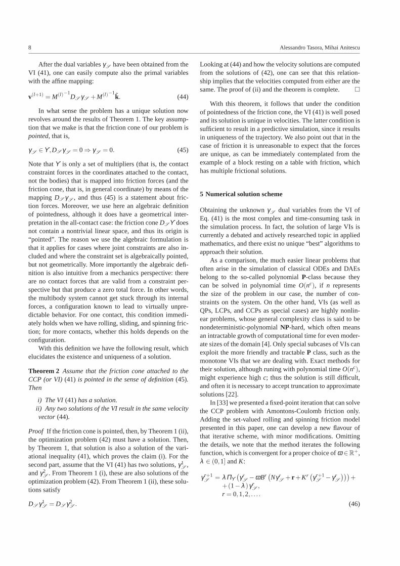
2.1 Rolling friction phenomena

ρ

Τ

Ν

Μ

Ν

ρ

R

ω ω

Fig. 1 Rolling friction. Two examples in the two-dimensional case.

Although the nonsmooth nature of the sliding frictionis evident in nature, because the friction force is abruptlyclamped to a maximum value as soon as the objects startsliding, the same sharpness is not evident in the experimen-tal observation of the rolling friction, because rolling frictioneffect increases smoothly as the rolling speeds increases.In

A complementarity-based rolling friction model for rigid contacts 3

fact, resistance to the rolling motion usually takes place be-cause in the contact area there may be inelastic deformationsof elasto-plastic materials [24]: the final outcome of this hys-teretic deformation is that the resultant of all pressures is al-ways placed a bit ahead of the position that it would take ifthe parts were not rolling.

Many classical textbooks about applied mechanics [37,8,26] describe a simplified model for this effect, consider-ing a rolling wheel of radiusR and expressing the displace-ment of the contact force by a singlefriction parameterρ,which has the dimension of length, or by a dimensionlesscoefficient of rolling friction fρ = ρ/R. The latter is alsomeant to allow an easy comparison with sliding friction:Given a normal forceN acting on a rolling disc, the hori-zontal force that is needed to keep it rolling at contant speedis T = fρN, (see Fig. 1), similar to the Coloumb sliding fric-tion case,T = fsN, with fs the coefficient of dry sliding fric-tion. Equivalently, the effect ofT on the disc can be replacedwith a tractive torqueM = TR, that is,M = fρNRor

M = ρN. (4)

This model is highly nonlinear because it states that thedisplacement, whose amount isρ regardless of the speed,has to change direction when the rolling speed changessign and must go to zero if there is no rolling speed. Thistristate model cannot be used practically within a general-purpose numerical simulation framework because scenariosoften occur where a sphere or a disc should come to restover a horizontal surface: since numerical roundoff consid-erations make impossible that the speed will be exactly null,the speed may actually oscillate around the null value, buteven small oscillations will change the sign of the rollingspeed and, consequently, also the displacement of the con-tact force will oscillate over the endpoints of the−ρ ,+ρinterval. The final result will be numerically unstable.

For this reason, we express the rolling friction model (4)as the following constraint with inequality

||M|| ≤ ρ ||N||, ||ωr ||(ρN−M) = 0, Mωr ≤ 0, (5)

whereωr is the rolling angular velocity, which must be op-posite to the rolling resistant momentM. The third conditionof Eq. (5) can also be written as〈M,ωr〉=−||M||||ωr ||.

Note that for whatever positive or negative rolling speed,this model corresponds to the classical rolling-friction model(4), but for the transition from steady state to moving stateitchanges the displacement in the[−ρ ,ρ ] limit. With this im-provement, the model can be seen as the counterpart of theAmontons-Coulomb friction model, because both can con-sider the static case.

2.2 Three dimensional rolling friction model

For extending the two-dimensional rolling friction modelto the generic case of contact between shapes in three-dimensional space, we introduce the following assumption

ASSUMPTION A1:The resisting torque is opposite tothe relative (rolling) angular velocity of the two bodies, ifany.

Although Assumption A1 is always verified for 2Dproblems, in some three-dimensional problems the resistingtorque can be misaligned with respect to the relative angu-lar velocity. See Appendix A for a derivation of the relativeangular velocity.

In cases with plane symmetry in the surroundings ofthe contact (for instance if the area of contact between tworolling bodies is an ellipse aligned to the rolling directionand the material properties are anisothropic), the speed ofdeformation of the material is symmetric with respect to theplane of rotation, thus resulting in a symmetric pressure dis-tribution at the area of contact, regardless of the type of vis-cous constitutive law of the material. In this case, Assump-tion A1 is always verified. This happens, for example, incase of spheres that are in contact, each with anisothropicmaterial, or in spheres that are rolling on flat surfaces.

Another special case that has much relevance in engi-neering applications is the contact between two surfaces thatcan be locally approximated as two cylinders with parallelaxes. This happens, for instance, in cam followers and inrollers over flat surfaces. In these cases, the torque is alignedto the rolling angular velocity.

In other situations, such as in the case of two genericellipsoids, the pressure distribution in the area of contact(that is elliptical and not necessarily with one of its mainaxes aligned to the direction of rolling) generates a normalreaction whose offset with respect to the plane of contactmight be not aligned to the direction of rolling, thus resultingin a resisting moment that is not exactly aligned to the vectorof the angular velocity.

Given theith contact, among two bodiesA andB, let ni

be the normal at the contact point, directed toward the exte-rior of theA body. Letui andwi be two vectors in the contactplane such thatni ,ui ,wi ∈ R

3 are mutually orthogonal vec-tors.

The signed gap functionΦ i represents the contact dis-tance. For each contact that is active (that isΦ i(·) = 0 be-cause bodies are touching), we introduce the contact forces,while inactive contacts (Φ i(·)> 0) do not enforce any reac-tion.

The normal contact force isFiN = γ i

nni , whereγ in ≥ 0 is

the multiplier that represents the modulus of the reaction.Friction force, if any, is represented by the multipliersγ i

u,

4 Alessandro Tasora, Mihai Anitescu

and γ iw which lead to the tangential component of the reac-

tion FiT = γ i

uui + γ iwwi .

Because of the inequalityγ in ≥ 0, the mathematical de-

scription of this unilateral model involves the Signorini com-plementarity problem [30]:

γ in ≥ 0 ⊥ Φ i(·)≥ 0. (6)

We introduce the rolling friction torque using the multi-pliers τ i

n, τ iu, andτ i

w, which correspond to a normal compo-nent of the torqueM i

N = τ inni and two tangential components

of the torqueM iT = τ i

uui + τ iwwi .

The normal component of the torqueM iN is responsible

for friction that reacts to spinning around the vertical axis,while the tangential componentM i

T = τ iuui + τ i

wwi is the ef-fect of the classical rolling friction. The model (5) is ex-tended to the three-dimensional case, the following inequal-ity holds for nonzero rolling velocity.∣∣∣∣M i

T

∣∣∣∣≤ ργ in

This corresponds to the inequalityρ i γ in ≥

√τ i

u2+ τ i

w2.

The rolling velocity vectorω iT is the part of the relative

angular velocity vectorω ir that lies on the contact plane, that

is, ω iT = ω i

r −ni⟨ω i

rni⟩; the condition that requiresω i

T tobe aligned and opposite toM i

T can be expressed as⟨M i

T ,ω iT

⟩=−

∣∣∣∣M iT

∣∣∣∣ ∣∣∣∣ω iT

∣∣∣∣ .

Therefore, the full rolling friction model for a contactwith rolling friction parameterρ i is mathematically equiva-lent to the following constraints:

ρ i γ in ≥

√τ i

u2+ τ i

w2

∣∣∣∣ω iT

∣∣∣∣(

ρ i γ in−

√τ i

u2+ τ i

w2)= 0,

⟨M i

T ,ω iT

⟩=−

∣∣∣∣M iT

∣∣∣∣ ∣∣∣∣ω iT

∣∣∣∣ .

(7)

Additionally, one can introduce the spinning friction,represented by a parameterσi , giving

σ i γ in ≥ τ i

n∣∣∣∣ω iN

∣∣∣∣(σ i γ in− τ i

n

)= 0,⟨

M iN,ω i

N

⟩=−

∣∣∣∣M iN

∣∣∣∣ ∣∣∣∣ω iN

∣∣∣∣ .(8)

Rolling contacts can be either sliding or not sliding.In the former case there could be also tangential forcescaused by dynamical friction; in the latter case there couldbe forces caused by sticking, the consequence of static fric-tion. Therefore we must introduce the Amontons-Coulombfriction model to take care of the tangential forces, eithersliding or static.

Within the classic theory of dry friction, the friction co-efficient µ i limits the ratio between the normal and the tan-gential force, and the tangential force must have a direction

that is opposite toviT , the tangential component of the rela-

tive velocityvir , if any, thus requiring

µ i γ in ≥

√γ iu

2+ γ iw

2

∣∣∣∣viT

∣∣∣∣(

µ i γ in−

√γ iu

2+ γ iw

2)= 0,

⟨Fi

T ,viT

⟩=−

∣∣∣∣FiT

∣∣∣∣ ∣∣∣∣viT

∣∣∣∣ .

(9)

3 The complete DVI model

The system state is defined by the vector of generalizedcoordinatesq ∈ R

mq and the vector of generalized speedsv ∈ R

mv. It might happen thatmq > mv because rotations ofrigid bodies in three-dimensional space are represented withunimodular quaternionsε ∈ H1 to avoid singularities in theparametrization ofSO(R,3); anyway it is straightforward todefine a (linear) mapq = Γ (q)v if q is needed.

We also introduce generalized force fieldsfe(q,v, t)and gyroscopic forcesfc(q,v) giving a total force fieldft(q,v, t) ∈ R

mv.The inertial properties of the system are represented by

the mass matrixM(q) ∈ Rmv×mv, assumed positive definite,

usually block-diagonal in the case of rigid bodies only.Bilateral constraints are introduced through a setB of

scalar constraint equations, assumed differentiable every-where:

Ψ i(q, t) = 0, i ∈ B. (10)

We introduce∇qΨ i =[∂Ψ i/∂q

]Tand∇Ψ iT =∇qΨ iT Γ (q),

to express the constraint (10) at the velocity level after dif-ferentiation:

dΨ i(q, t)dt

= ∇Ψ iT v+∂Ψ i

∂ t= 0, i ∈ B. (11)

Frictional unilateral contacts define a setA . For eachcontacti ∈ A , we introduce the tangent space generatorsDi

γu, Di

γw, Di

τu, Di

τw, Di

τn∈ R

mv; for details about their for-mulation, see Appendix B.

Another way to write (7), (8), and (9) is to use the max-imum dissipation principle, thus leading respectively to thefollowing constraints on the dynamic equilibrium

(τ i

u, τ iw

)= argminvT

(Di

τuτ i

u+Diτw

τ iw

)

s.t.(τ iu, τ i

w) ∈ Z ir

Z ir

∆=

{(τ i

u, τ iw)|

√τ i

u2+ τ i

w2≤ ρ i γ i

n

} (12)

(τ i

n

)= argminvT

(Di

τnτ i

n

)

s.t. τ in ∈ Z i

s

Z is

∆=

{τ i

n| |τ in| ≤ σ i γ i

n

} (13)

(γ iu, γ i

w

)= argminvT

(Di

γuγ iu+Di

γwγ iw

)

s.t.(γ iu, γ i

w) ∈ Z if

Z if

∆=

{(γ i

u, γ iw)|

√γ iu

2+ γ i

w2≤ µ i γ i

n

} (14)

A complementarity-based rolling friction model for rigid contacts 5

Here, Z ir , Z i

s , and, respectively,Z if , are the rolling,

spinning, and respectively, friction cone sections. Alterna-tively, for the case where the tangential rolling torques isnotzero, we derive the Fritz John optimality conditions for thenonlinear program (12),

s=∇τu,τwvT (Dτuτ iu+Dτw τ i

w

)+

−λω ∇τu,τw

(ργ i

n−

√τ i

u2+ τ i

w2)= 0 (15)

ρ i γ in−

√τ i

u2+ τ i

w2≥ 0, ⊥ λω ≥ 0. (16)

When the tangential rolling torques are zero, the functionsdefiningZ i

r , are not differentiable so the above derivationdoes not hold. However, for purposes of exposing our for-mulation we will assume the opposite the case, and in laterdevelopments (40) we remove this assumptions by usingcone polar formalisms.

The same derivation can be performed for (12) and (13);hence the complete model, including inertial effects, forcefields, bilateral constraints, unilateral contacts with friction,rolling friction, and spinning friction, is the following dif-ferential variational inequality

q = Γ (q)v

M(q)dvdt

= ∑i∈A

(γ inDi

γn+ γ i

uDiγu+ γ i

wDiγw+

+τ inDi

τn+ τ i

uDiτu+ τ i

wDiτw

)+

+ ∑i∈B

γ iB∇Ψ i + ft(t,q,v)

i ∈ B : Ψ i(q, t) = 0i ∈ A : γ i

n ≥ 0 ⊥ Φ i(q)≥ 0∇τu,τwvT

(Dτu τ i

u+Dτw τ iw

)+

−λ iω ∇τu,τw

(ρ i γ i

n−

√τ i

u2+ τ i

w2)= 0

ρ i γ in−

√τ i

u2+ τ i

w2≥ 0, ⊥ λ i

ω ≥ 0∇γu,γwvT

(Dγu γ i

u+Dγw γ iw

)+

−λ iv∇γu,γw

(µ i γ i

n−

√γ iu

2+ γ iw

2)= 0

µ i γ in−

√γ iu

2+ γ i

w2≥ 0, ⊥ λ i

v ≥ 0∇τnvT

(Dτnτ i

n

)+

−λ iτ ∇τn

(σ i γ i

n−|τ in|)= 0

µ i γ in−|τ i

n| ≥ 0, ⊥ λ iτ ≥ 0

(17)

The former DVI can be discretized in time. Using a timesteph, posingγ = hγ , and adopting the exponential mapΛ(·) described in [33] to allow direct integration on the Lie

group, we have the following problem.

q(l+1) = Λ(q(l),v(l+1),h)

Mv(l+1) = ∑i∈A

(γ inDi

γn+ γ i

uDiγu+ γ i

wDiγw+

+τ inDi

τn+ τ i

uDiτu+ τ i

wDiτw

)+

+ ∑i∈B

γ iB∇Ψ i +hft(t,q,v)+Mv(l)

i ∈ B :1h

Ψ i(q(l))+∇Ψ iT v(l+1)+∂Ψ i

∂ t= 0

i ∈ A : γ in ≥ 0 ⊥ 1

hΦ i(q(l))+∇Φ iT v(l+1) ≥ 0∇τu,τwvT

(Dτuτ i

u+Dτwτ iw

)+

−λ iω ∇τu,τw

(ρ iγ i

n−

√τ i

u2+ τ i

w2)= 0

ρ iγ in−

√τ i

u2+ τ i

w2 ≥ 0, ⊥ λ i

ω ≥ 0∇γu,γwvT

(Dγuγ i

u+Dγwγ iw

)+

−λ iv∇γu,γw

(µ iγ i

n−

√γ iu

2+ γ iw

2)= 0

µ iγ in−

√γ iu

2+ γ iw

2 ≥ 0, ⊥ λ iv ≥ 0

∇τnvT(Dτnτ i

n

)+

−λ iτ ∇τn

(σ iγ i

n−|τ in|)= 0

µ iγ in−|τ i

n| ≥ 0, ⊥ λ iτ ≥ 0

(18)

This is a mixed nonlinear complementarity problem,whose solution is not guaranteed to exist. Indeed, most exis-tence results require monotonicity of the mapping definingthe complementarity problem. In turn, this implies convexityof the solution set of the nonlinear complementarity prob-lem [10]. Unfortunately, not even the weaker condition ofthe convexity of the solution set can be guaranteed. Indeed,it has been already shown that, for the subcase of a linearcomplementarity problem (LCP) corresponding to a simplepyramidal frictional model, the solution set may be noncon-vex [1]. This situation can occur only if the mapping of theLCP is nonmonotone, which in the linear case implies thatits matrix is not positive semi-definite.

4 Casting to a convex solvable problem

In the following we show that, under mild conditions, theoriginal problem can be relaxed as a monotone cone com-plementarity problem (CCP) that guarantees existence ofthe solution and convexity of the solution set. The prob-lem is equivalent to a convex optimization problem, a feasi-ble quadratic programming problem (QP) with conical con-straints. We note that while one cannot guarantee uniquenessof the solution of the CCP (indeed, lack of uniqueness ofthe forces is known to appear even in frictionless cases thatare linear and convex problems), one can guarantee undersome mild assumptions uniqueness of the velocity solution[3]. The latter condition is sufficient for a predictive time-stepping scheme to exist.

6 Alessandro Tasora, Mihai Anitescu

Assume that for each contacti ∈A we define the vectorof wrench reactions

γ iA =

{γ in,γ i

u,γ iw,τ i

n,τ iu,τ i

w

}T

and the corresponding twist of local linear and angularvelocities in the contact point, plus the stabilization term1hΦ(q), that is,

uiA =

{∇Φ i,Tv+ 1

hΦ i ,Di,Tγu v,Di,T

γv v,Di,Tτn v,Di,T

τu v,Di,Tτw v

}T.

In the rest of this section we omit thei indexes for compact-ness.

We differentiate the Fritz John optimality conditions(15) obtaining, for the rolling friction part,

vTDτu = λω τu1√

τ2u + τ2

w

(19)

vTDτw = λω τw1√

τ2u + τ2

w

. (20)

Then,

λω =√(DT

τuv)2+(DT

τwv)2. (21)

Note that for the sliding friction one gets similar results,vTDγu = λvγu1/

√γ2u + γ2

w and vTDγw = λvγw1/√

γ2u + γ2

w,

with λv =√(DT

γuv)2+(DT

γwv)2; whereas for the spinning

friction vTDτn = λτ τn/|τn|, with λτ = DTτn

v|τn|/τn.Now, the inner product for the complementarity in the

optimality condition requires that

λω

(ργn−

√τ2

u + τ2w

)= 0

λω

√τ2

u + τ2w = λω ργn. (22)

Similarly one can derive, for sliding and spinning,

λv

√γ2u + γ2

w = λvµγn (23)

λτ |τn|= λτ σγn. (24)

If we assume the orthogonality ofγA anduA , we have

〈γA ,uA 〉=γn(∇ΦTv+ 1hΦ)+ γuDT

γuv+ γwDT

γwv+

+ τnDTτn

v+ τuDTτu

v+ τwDTτw

v = 0. (25)

By adding a relaxation termAr for the normal velocity,the orthogonality condition for unilateral contact in the dis-cretized DVI (18) becomes

γn ≥ 0 ⊥ 1hΦ +∇ΦTv+Ar ≥ 0.

Since complementarity implies nullity of inner product, wethen have

γn(

1hΦ +∇ΦTv

)=−γnAr ≥ 0. (26)

By exploiting (26), (19), (20), and so forth, recalling thatx2/|x|= |x|, with simple algebraic manipulation, we rewrite(25) as

〈γA ,uA 〉=− γnAr +γ2uλv√

γ2u + γ2

w

+γ2wλv√

γ2u + γ2

w

+

+τ2

uλω√τ2

u + τ2w

+τ2

wλω√τ2

u + τ2w

+τ2

nλτ|τn|

= 0

γnAr =λv

√γ2u + γ2

w+λω

√τ2

u + τ2w+λτ |τn|. (27)

By substituting (22), (23), and (24) in (27), and by simplify-ing γn, we have that the relaxation term that allows orthogo-nality of γ ’s andu’s is, for theith contacti ∈ A ,

Air =µ i

√(Di

γuv)2+(Di

γwv)2+

+ρ i√

(Diτu

v)2+(Diτw

v)2+σ i |Diτn

v|. (28)

The introduction of theAir term has the drawback of

modifying the contact constraint; from a practical point ofview there is the side effect that the gap between objects in-crease with the sliding speed instead of remaining equal tozero; this effect has been discussed in [33] for the simplecase of sliding friction. Now, introducing also rolling andspinning friction, one can see from Eq. (28) that rotational

motion increases the gap (the√(Di

τuv)2+(Di

τwv)2 term is

also the norm ofω iT ), and that the increase is always di-

rected outward. This is the price for having convexified theoriginal problem. In many situations this can be acceptable,indeed one can demonstrate that at steady state, i.e. when∇Φ iTv = 0 in (26), the separation gapΦ i decreases withlow speeds, lowµ , ρ, σ , and small timesteps.

We note that if we plan to use rolling friction to simulategranular material, the above mentioned side effect of therelaxation leads to a dilatancy effect that really happens inphysical world.

Aiming at a generic compact notation, we now introducebi

A∈ R

6 = {1hΦ i ,0,0,0,0,0}T , and we build the following

aggregate vectorsbA ∈ R6nA , γA ∈ R

6nA , uA ∈ R6nA :

bA ={

b1,TA

,b2,TA

, . . . ,bnA ,TA

}T,

γA ={

γ1,TA

,γ2,TA

, . . . ,γnA ,TA

}T,

uA ={

u1T

A,u2T

A, . . . ,unA ,T

A

}T.

(29)

For each contact we can define a matrix with six columns,

Di =[∇Φ i |Di

γu|Di

γw|Di

τn|Di

τu|Di

τw

], (30)

and a six-dimensional cone that defines the set of admissiblereactions in the sliding, rolling, spinning friction contact:

Zi =

γ ∈ R

6

∣∣∣∣∣∣

µ iγn ≥√

γ2u + γ2

w,

ρ iγn ≥√

τ2u + τ2

w,

σ iγn ≥ |τn|

. (31)

A complementarity-based rolling friction model for rigid contacts 7

Similarly, for bilateral constraints, we havebB ∈ RnB ,

andγB ∈ RnB :

bB ={

1hΨ 1+ ∂Ψ1

∂ t , 1hΨ 2+ ∂Ψ2

∂ t , . . . , 1hΨnB + ∂ΨnB

∂ t

}T

γB ={

γ1B,γ2

B, . . . ,γnB

B

}T

uB ={

u1B,u2

B, . . . ,unB

B

}T.

(32)

The complete aggregate vectors and matrices of the en-tire system are

γS ={

γTA ,γT

B

}T, uS =

{uT

A ,uTB

}T, bS =

{bT

A ,bTB

}T,

(33)

DS =[Di1|Di2| . . . |DinA |∇Ψ1|∇Ψ2| . . . |∇Ψ nB

]. (34)

Moreover we define the product of all the sliding androlling friction cones and the possible values of reactionsinbilateral constraints as

ϒ =(×i∈A Z

i)× (×i∈BR) (35)

and its polar (note thatR◦ = {0}):

ϒ ◦ =(×i∈A Z

i◦)× (×i∈B{0}) . (36)

Now we proceed with a simplification by introducing

k(l)= M(l)v(l)+hft(t(l),q(l),v(l)). (37)

From the relaxed version of (18) one can see thatuS =

NγS + r , where

N = DTS M(l)−1

DS (38)

r = DTS M(l)−1

k +bS . (39)

The entire system is described by the following CCP:

(NγS + r) ∈ −ϒ ◦ ⊥ γS ∈ϒ . (40)

The CCP (40) is also equivalent to a variational inequal-ity as expressed in the VI of Eq (1), namely

γS ∈ϒ : 〈NγS + r ,y− γS 〉 ≥ 0 ∀y ∈ϒ . (41)

Several theoretical results for (41) can be obtained bynoting that it is related to the following optimization prob-lem.

minγS ∈ϒ

12

γTS NγS + rTγS (42)

Theorem 1 Consider the variational inequality(41) andthe optimization problem(42). Then the following state-ments hold:

i) If (42) has a solution, then that solution satisfies thevariational inequality(41). Conversely, any solution of(41) is a solution of(42).

ii) Either (42)has a solution, or there existsγS such thatDS γS = 0.

iii) If (42) has two solutionsγ1S

andγ2S

, then they mustsatisfy DS γ1

S= DS γ2

S.

Proof If (42) has a solution, then since the constraintsϒare convex, they must satisfy the Kuhn-Tucker conditions,which are simply the statement of (41). Conversely, becauseof the convexity of the coneϒ and of the objective function,any Kuhn-Tucker solution is a global solution, which provesPart (i).

For Part (ii), if the objective function of (42) is boundedbelow over the convex setϒ , it follows that the problem (42)must have a solution. Assume that this is not the case, that is,that there exists a sequenceγn

S∈ϒ , n= 0,1,2, . . . such that

12γnT

SNγn

S+ rTγn

S→−∞. Because of the continuity of the

objective function, such a sequence must satisfy∣∣∣∣γn

S

∣∣∣∣→∞(otherwise the objective function would stay bounded). Inparticular, this implies that

12

γnTS Nγn

S + rTγnS ≤ 0;∀n≥ n0 (43)

for some integern0. Define the scaled vectorγnS =

γnS

||γnS ||

∈

ϒ . Since the scaled vector sequence is in the unit ball, whichis compact, it must have a limit point, which we denote byγ∗S . We assume, without loss of generality, that the entire

sequence converges to this point. Dividing (43) by∣∣∣∣γn

S

∣∣∣∣2and taking the limit, we have that the second term goes to 0,and we obtain

12

γ∗TS Nγ∗S .≤ 0

Using the expression forN, (38), and the fact that the massmatrix is positive definite, this implies thatDS γ∗S = 0,which in turn proves Part (ii) of the theorem.

For Part (iii), assume that there are two solutions of theoptimization problem (42),γ1

Sand γ2

S. Then, by the fact

that the objective function is convex and that the constraintsare convex, for anyt ∈ [0,1], we have thatγ1

S+ t(γ2

S− γ1)

is also a solution of (42). That is, the objective function value

(γ1

S + t(γ2S − γ1)

)TN(γ1

S + t(γ2S − γ1)

)+

+rT (γ1S + t(γ2

S − γ1))

is constant int. This function is a quadratic, and this canoccur only if the coefficient int2 is 0, that is,

(γ2

S − γ1)TN(γ2

S − γ1)= 0.

Again using the expression forN, (38), and the fact that themass matrix is positive definite, this implies thatDS (γ1

S −

γ1S ) = 0, which in turn proves Part (iii) of the theorem. The

proof of the theorem is complete. �

8 Alessandro Tasora, Mihai Anitescu

After the dual variablesγS have been obtained from theVI (41), one can easily compute also the primal variableswith the affine mapping:

v(l+1) = M(l)−1DS γS +M(l)−1

k. (44)

In what sense the problem has a unique solution nowrevolves around the results of Theorem 1. The key assump-tion that we make is that the friction cone of our problem ispointed, that is,

γS ∈ϒ ,DS γS = 0⇒ γS = 0. (45)

Note thatϒ is only a set of multipliers (that is, the contactconstraint forces in the coordinates attached to the contact,not the bodies) that is mapped into friction forces (and thefriction cone, that is, in general coordinate) by means of themappingDS γS , and thus (45) is a statement about fric-tion forces. Moreover, we use here an algebraic definitionof pointedness, although it does have a geometrical inter-pretation in the all-contact case: the friction coneDSϒ doesnot contain a nontrivial linear space, and thus its origin is“pointed”. The reason we use the algebraic formulation isthat it applies for cases where joint constraints are also in-cluded and where the constraint set is algebraically pointed,but not geometrically. More importantly the algebraic defi-nition is also intuitive from a mechanics perspective: thereare no contact forces that are valid from a constraint per-spective but that produce a zero total force. In other words,the multibody system cannot get stuck through its internalforces, a configuration known to lead to virtually unpre-dictable behavior. For one contact, this condition immedi-ately holds when we have rolling, sliding, and spinning fric-tion; for more contacts, whether this holds depends on theconfiguration.

With this definition we have the following result, whichelucidates the existence and uniqueness of a solution.

Theorem 2 Assume that the friction cone attached to theCCP (or VI) (41) is pointed in the sense of definition(45).Then

i) The VI (41)has a solution.ii) Any two solutions of the VI result in the same velocityvector(44).

Proof If the friction cone is pointed, then, by Theorem 1 (ii),the optimization problem (42) must have a solution. Then,by Theorem 1, that solution is also a solution of the vari-ational inequality (41), which proves the claim (i). For thesecond part, assume that the VI (41) has two solutions,γ1

S,

andγ2S

. From Theorem 1 (i), these are also solutions of theoptimization problem (42). From Theorem 1 (ii), these solu-tions satisfy

DS γ1S = DS γ2

S .

Looking at (44) and how the velocity solutions are computedfrom the solutions of (42), one can see that this relation-ship implies that the velocities computed from either are thesame. The proof of (ii) and the theorem is complete. �

With this theorem, it follows that under the conditionof pointedness of the friction cone, the VI (41) is well posedand its solution is unique in velocities. The latter condition issufficient to result in a predictive simulation, since it resultsin uniqueness of the trajectory. We also point out that in thecase of friction it is unreasonable to expect that the forcesare unique, as can be immediately contemplated from theexample of a block resting on a table with friction, whichhas multiple frictional solutions.

5 Numerical solution scheme

Obtaining the unknownγS dual variables from the VI ofEq. (41) is the most complex and time-consuming task inthe simulation process. In fact, the solution of large VIs iscurrently a debated and actively researched topic in appliedmathematics, and there exist no unique “best” algorithms toapproach their solution.

As a comparison, the much easier linear problems thatoften arise in the simulation of classical ODEs and DAEsbelong to the so-called polynomialP-class because theycan be solved in polynomial timeO(nc), if n representsthe size of the problem in our case, the number of con-straints on the system. On the other hand, VIs (as well asQPs, LCPs, and CCPs as special cases) are highly nonlin-ear problems, whose general complexity class is said to benondeterministic-polynomialNP-hard, which often meansan intractable growth of computational time for even moder-ate sizes of the domain [4]. Only special subcases of VIs canexploit the more friendly and tractableP class, such as themonotone VIs that we are dealing with. Exact methods fortheir solution, although runing with polynomial timeO(nc),might experience highc; thus the solution is still difficult,and often it is necessary to accept truncation to approximatesolutions [22].

In [33] we presented a fixed-point iteration that can solvethe CCP problem with Amontons-Coulomb friction only.Adding the set-valued rolling and spinning friction modelpresented in this paper, one can develop a new flavour ofthat iterative scheme, with minor modifications. Omittingthe details, we note that the method iterates the followingfunction, which is convergent for a proper choice ofω ∈R

+,λ ∈ (0,1] andK:

γ r+1S

= λΠϒ(γ r

S−ωBr

(Nγ r

S+ r +Kr

(γ r+1

S− γ r

S

)))+

+(1−λ )γ rS,

r = 0,1,2, . . . .

(46)

A complementarity-based rolling friction model for rigid contacts 9

TheΠϒ operator is a projection ontoϒ , so thatΠϒ (γ) =argminζ∈ϒ ||γ − ζ ||. Given the separable cone structure ofΠϒ as defined in Eq. (35), the computation ofΠϒ (γ) canbe split intonA projectionsΠ i

Z(γ i) and intonB identities

(no projections are required for the bilateral constraints).The originalΠ i

Z(γ i) projection discussed in [33] operates

only on the three values of the reactions that must obeythe Amontons-Coulomb friction. In the advanced case, how-ever, that includes also rolling friction and spinning fric-tion one must map the six-dimensional wrench onto the six-dimensional coneZ defined in Eq. (31), soΠ i

Z(γ i) : R6 →

R6. See Appendix C for details about this projection.

Given the requirement of solving a VI for each timestep,the DVI approach appears to be less competitive than theclassic DEM concept of regularizing nonsmooth phenomenavia smooth but stiff force fields, because DEMs lead to un-coupled equations of motion of ODE type with basic linearO(nb) complexity for each timestep. However, our DVI set-ting permits large timesteps because it does not suffer fromthe stability issues implied by stiff forces in DEMs, so theincreased workload for each timestep is paid back by fewertimesteps being required [32].

We remark that a parallel version of this rolling and spin-ning friction model can be easily implemented on parallelhardware of GPU type, as described in [34], and on hybridhigh-performance computers [21].

6 Examples

6.1 Comparison against analytical solution

A simple validation against the analytical solution for arolling disk is presented here. We consider a rolling diskwith radiusR = 1 m, massM = 10 kg, moment of iner-tia J = 4 kgm2, initial positionx|t=0 = 0 m initial horizon-tal speed on x axisvx|t=0 = 1 m/s, initial angular veloc-ity ω|t=0 = −1 rad/s. We use a rolling friction parameterρ = 0.02 m and a sliding/static friction coefficientµ = 0.9.The gravity acceleration isgy =−9.8 m/s2

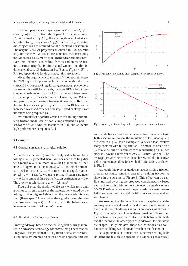
Figure 2 plots the motion of the disk which rolls untilit comes to a rest because of the deceleration caused by therolling friction. Figure 3 shows that the deceleration is con-stant (linear speed) in analytical theory, which uses the con-stant resistant torqueTr = M ·gy ·ρ ; a similar behavior canbe seen in the results of the DVI model.

6.2 Simulation of a linear guideway

Linear guideways based on recirculating ball bearings repre-sent an advanced technology for constraining linear motion.They avoid the problem of sliding friction between the trans-lating parts by interposing rows of rolling spheres that can

0 1 2 3 4 5 60

0.5

1

1.5

2

2.5

3

t [s]

x [m

]

DVIanalytic

Fig. 2 Motion of the rolling disk: comparison with classic theory.

0 1 2 3 4 5 6

0

0.2

0.4

0.6

0.8

1

t [s]

v x [m/s

]

DVIanalytic

Fig. 3 Velocity of the rolling disk: comparison with classic theory.

recirculate back in enclosed channels, like tracks in a tank.In this section we present the simulation of the linear systemdepicted in Fig. 4, as an example of a device that involvesmany contacts with rolling friction. The model is based on a35 mm wide rail, with four rows of recirculating balls, eachsteel ball having a diameter of 2Rb = 6.4 mm. Nine balls, onaverage, provide the contact in each row, and the four rowsdefine four contact directions with 45◦ orientation, as shownin Fig. 5.

Although this type of guideway avoids sliding friction,a small resistance remains, caused by rolling friction, asshown in the scheme of Figure 6. This effect can be eas-ily simulated by using the proposed complemetarity-basedapproach to rolling friction: we modeled the guideway in a3D CAD software, we saved the parts using a custom trans-lation software, we imported the file in our software, and wesimulated it.

We assumed that the contact between the spheres and theraceways is always aligned to the 45◦ direction, so we intro-duced eight stretched boxes as collision shapes, as shown inFig. 7; in this way the collision algorithm of our software canautomatically compute the contact points between the ballsand the raceways. In other types of guideways, the racewaysare shaped like gothic arcs: these can be modeled as well,but such nodeling would not add much to the discussion.

No significant side contact occurs between rolling balls(in some models plastic spacers exclude this posssibility),

10 Alessandro Tasora, Mihai Anitescu

Recirculating balls

Upper contact balls

Lower contact balls

Sliding block

and scraper

Support flange

Seals

Rail

Fig. 4 The simulated linear guideway, with the scheme of the recircu-lating balls.

N

N' N''

Fig. 5 Section of the linear guideway, showing the contact betweenballs and grooves.

ρ

ω

v

R R

n

n+1Rn n+2

O

Fig. 6 Schematic representation of the forces acting on the rollingballs.

and we did not consider static preload, although it could besimulated as well.

Since the system has many more contact constraintsthan needed, the indeterminacy is solved by introducing aTikhonov regularization: from a numerical point of view thismeans adding a nonzero diagonalC to theN matrix of Eq.38, that is,NTyk = N+C. From a mechanical point of view,the Tikhonov regularization means that we introduce com-

Rail collision shapes

Block collision shapes

Balls

Contacts

Fig. 7 Collision primitives used in the simulation.

−0.04 −0.02 0.00 0.02 0.04

vx [m/s]

−10

−5

0

5

10

Fx [N]

ρ=0.004

ρ=0.005

ρ=0.006

ρ=0.004, seals

ρ=0.005, seals

ρ=0.006, seals

Fig. 8 Resisting forceFx for different values of rolling friction pa-rameterρ , with and without the effect of seal friction (case of loadFy = 490N)

pliance in contacts; in detail, we generateC from the in-verses of the stiffness values in contact points, as computedby the Hertz-Mindlin theory.

The manufacturer of the guideway provides the follow-ing formula for estimating the resistance to horizontal slid-ing at low speeds:Fx =−sign(vx)(ζFy+S), whereFy is thenormal load,ζ is typically about 0.005, andS is the forcecaused by the sliding friction of seals and scrapers, in ourcaseS= 5.3N. Such friction is introduced in our modelby using a convex box-constraint of the type−S≤ γS ≤ S,whose effect on the DVI is similar to the already discussed,and more complex, contact constraints. The effect of theζFy

term comes from the simulation of the many rolling con-tacts, each with a rolling friction parameterρ = ζRb. Resultsfrom the simulations show precise agreement with the aboveformula, as shown in Fig. 8. For zero speed, the model isable to describe also the sticking effect that, although mod-est, can be measured on this class of devices.

6.3 Application to the simulation of granular materials

The mechanics of granular matter has became a fertile re-search topic only recently, because of the vast computationalresources that are required. One of the fields that would ben-

A complementarity-based rolling friction model for rigid contacts 11

efit from advances in this area is pharmaceutical engineer-ing, where multibody dynamics could be used to study pro-cesses that involve powders: milling, blending, granulation,compression, and coating [17]

In the popular discrete element method (DEM), the bulkmaterial is discretized in many particles with unilateral fric-tional contacts [7]. Various micromechanical contact modelsare available in the DEM field in order to define the interac-tion between the particles; in most cases, the nonsmooth na-ture of contact means that those models always produce stiffcontact forces, and hence, that short integration timestepsare needed.

The need of rolling friction in granular simulationsis motivated by experimental evidence; for example [23]shows that rolling resistance can have marked influence onthe mechanics of particle assemblies at microscales; in somecases, its effect can be more relevant than interparticle slid-ing friction [36]. Rolling friction has been shown to affectonly marginally the elastic properties of granular assem-blies, but other collective phenomena such as shear resis-tance and dilatancy are significantly affected [5].

In some cases the simple inhibition of particle rotationsin DEM algorithms can improve the solution with respectto the case of free frictionless rotation [6]. During the pastfew years, more sophisticated models of rolling friction havebeen proposed for interparticle contacts, for example in [14].Given the difficulty of tuning the parameters of complexmodels, approaches based on few parameters such as theapproach of [15] are welcome.

To some extent, the macroscopic effect of rolling frictionin granular media is simular to the effect of dealing withnonspherical particles [19].

The collective behavior of particles with irregular andfaceted shapes is different from the behavior of sphericalparticles, even if granular assemblies share the same granu-lometry and friction; in general, oddly shaped particles tendto generate less deformable assemblies when compared withspherical particles of equal size [35]. Of course, a straight-forward approach could take into account the simulation ofall the detailed shapes, but this would lead to high simulationtimes, both because there will be multiple contacts betweenpairs of particles and because the collision detection phasewould require more RAM and CPU time to process thosecontacts.

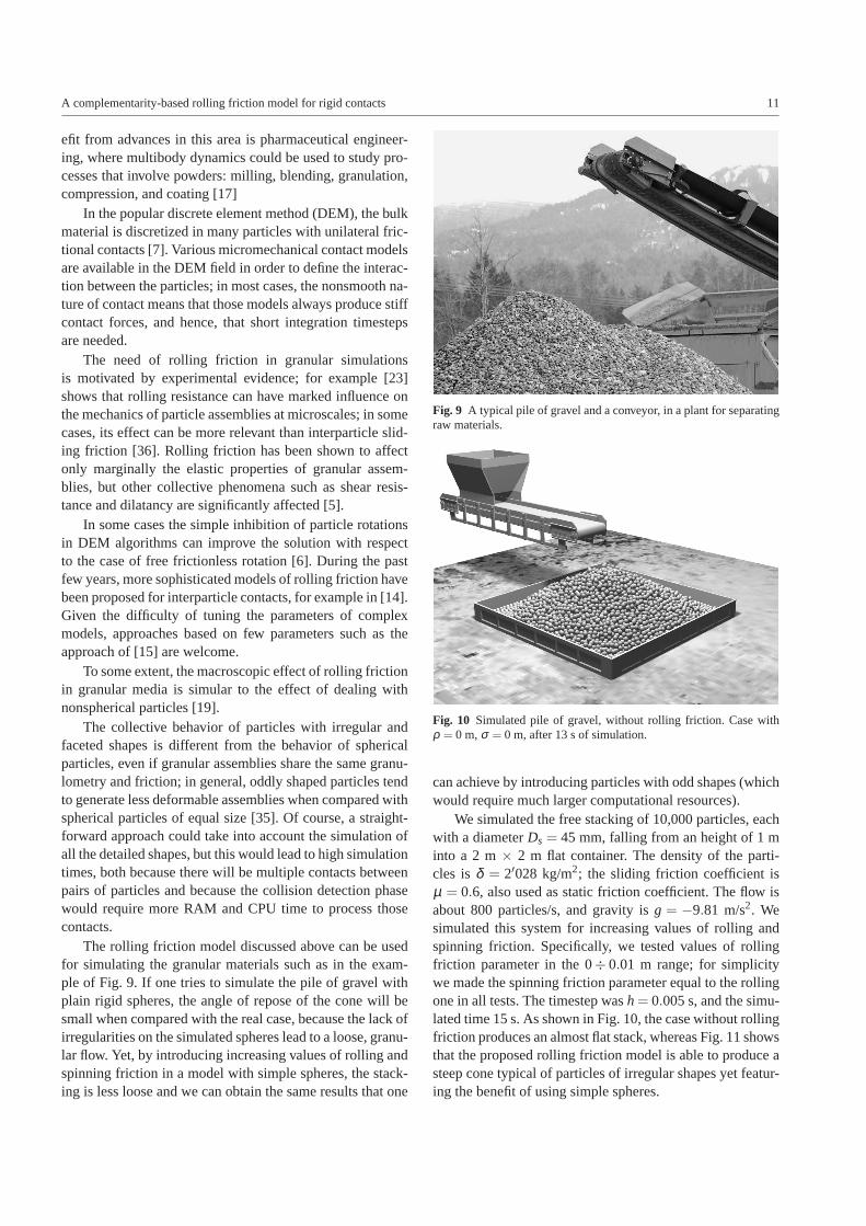
The rolling friction model discussed above can be usedfor simulating the granular materials such as in the exam-ple of Fig. 9. If one tries to simulate the pile of gravel withplain rigid spheres, the angle of repose of the cone will besmall when compared with the real case, because the lack ofirregularities on the simulated spheres lead to a loose, granu-lar flow. Yet, by introducing increasing values of rolling andspinning friction in a model with simple spheres, the stack-ing is less loose and we can obtain the same results that one

Fig. 9 A typical pile of gravel and a conveyor, in a plant for separatingraw materials.

Fig. 10 Simulated pile of gravel, without rolling friction. Case withρ = 0 m,σ = 0 m, after 13 s of simulation.

can achieve by introducing particles with odd shapes (whichwould require much larger computational resources).

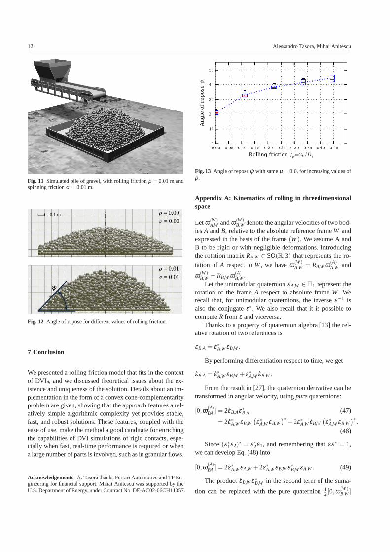
We simulated the free stacking of 10,000 particles, eachwith a diameterDs = 45 mm, falling from an height of 1 minto a 2 m× 2 m flat container. The density of the parti-cles isδ = 2′028 kg/m2; the sliding friction coefficient isµ = 0.6, also used as static friction coefficient. The flow isabout 800 particles/s, and gravity isg = −9.81 m/s2. Wesimulated this system for increasing values of rolling andspinning friction. Specifically, we tested values of rollingfriction parameter in the 0÷ 0.01 m range; for simplicitywe made the spinning friction parameter equal to the rollingone in all tests. The timestep wash= 0.005 s, and the simu-lated time 15 s. As shown in Fig. 10, the case without rollingfriction produces an almost flat stack, whereas Fig. 11 showsthat the proposed rolling friction model is able to produce asteep cone typical of particles of irregular shapes yet featur-ing the benefit of using simple spheres.

12 Alessandro Tasora, Mihai Anitescu

Fig. 11 Simulated pile of gravel, with rolling frictionρ = 0.01 m andspinning frictionσ = 0.01 m.

ψψψψ

ρ = 0.00 σ = 0.00

ρ = 0.01 σ = 0.01

= 0.1 m

Fig. 12 Angle of repose for different values of rolling friction.

7 Conclusion

We presented a rolling friction model that fits in the contextof DVIs, and we discussed theoretical issues about the ex-istence and uniqueness of the solution. Details about an im-plementation in the form of a convex cone-complementarityproblem are given, showing that the approach features a rel-atively simple algorithmic complexity yet provides stable,fast, and robust solutions. These features, coupled with theease of use, make the method a good canditate for enrichingthe capabilities of DVI simulations of rigid contacts, espe-cially when fast, real-time performance is required or whena large number of parts is involved, such as in granular flows.

Acknowledgements A. Tasora thanks Ferrari Automotive and TP En-gineering for financial support. Mihai Anitescu was supported by theU.S. Department of Energy, under Contract No. DE-AC02-06CH11357.

0.00 0.05 0.10 0.15 0.20 0.25 0.30 0.35 0.40 0.45

Rolling friction fρ=2ρ/Ds

0

10

20

30

40

50

Angle of repose

ψ

Fig. 13 Angle of reposeψ with sameµ = 0.6, for increasing values ofρ.

Appendix A: Kinematics of rolling in threedimensionalspace

Let ω(W)A,W andω(W)

B,W denote the angular velocities of two bod-iesA andB, relative to the absolute reference frameW andexpressed in the basis of the frame(W). We assume A andB to be rigid or with negligible deformations. Introducingthe rotation matrixRA,W ∈ SO(R,3) that represents the ro-

tation of A respect toW, we haveω(W)A,W = RA,Wω(A)

A,W and

ω(W)B,W = RB,Wω(A)

B,W.Let the unimodular quaternionεA,W ∈ H1 represent the

rotation of the frameA respect to absolute frameW. Werecall that, for unimodular quaternions, the inverseε−1 isalso the conjugateε∗. We also recall that it is possible tocomputeR from ε and viceversa.

Thanks to a property of quaternion algebra [13] the rel-ative rotation of two references is

εB,A = ε∗A,WεB,W.

By performing differentiation respect to time, we get

εB,A = ε∗A,WεB,W + ε∗A,WεB,W.

From the result in [27], the quaternion derivative can betransformed in angular velocity, usingpurequaternions:

[0,ω(A)BA ] = 2εB,Aε∗B,A (47)

= 2ε∗A,WεB,W(ε∗A,WεB,W

)∗+2ε∗A,WεB,W

(ε∗A,WεB,W

)∗.

(48)

Since(ε∗1ε2)∗ = ε∗2ε1, and remembering thatεε∗ = 1,

we can develop Eq. (48) into

[0,ω(A)BA ] = 2ε∗A,WεA,W +2ε∗A,WεB,Wε∗B,WεA,W. (49)

The productεB,Wε∗B,W in the second term of the suma-

tion can be replaced with the pure quaternion12[0,ω

(W)B,W]

A complementarity-based rolling friction model for rigid contacts 13

using Eq. (47). Also, the first term can be premultipliedby ε∗A,WεA,W = 1, becoming 2ε∗A,WεA,Wε∗A,WεA,W; here theproduct between the second and third quaternion can be re-

placed with the pure quaternion12[0,ω(W)A,W]∗, again using Eq.

(47). Thus we have

[0,ω(A)BA ] = ε∗A,W[0,ω(W)

A,W]∗εA,W + ε∗A,W[0,ω(W)B,W]εA,W. (50)

A rotation in 3D space of the vector part of a purequaternion can be obtained with unitary quaternions, that is,[0,v(W)] = εA,W[0,v(A)]ε∗A,W.

Hence, recalling that[0,ω(W)A,W]∗ = −[0,ω(W)

A,W] by theproperty of conjugate quaternions, we can rewrite Eq. (50)and obtain the expected result for relative angular velocityω r :

[0,ω(A)BA ] =−[0,ω(A)

A,W]+ [0,ω(A)B,W]

ω(A)BA = ω(A)

B,W −ω(A)A,W. (51)

Appendix B: Formulation of D vectors

We assume that the vector of generalized velocitiesv con-tains the speeds of the centers of mass of the bodiesx(W), ex-pressed in absolute coordinates(W) and the angular veloc-ities ω(i) expressed in the local coordinates of theith body,

asv =[x(W)

1 ,ω(1)1 , x(W)

2 ,ω(2)2 , . . . ,

]T.

Given a contact between a pair of two rigid bodiesAand B, we define the positions of the two contact pointswith respect to the centers of mass, expressed in the coor-

dinate systems of the two bodies, ass(A)A ands(B)B . The ab-solute rotations of the coordinate systems of the bodies are

R(W)A ,R(W)

B ∈ SO(R,3) and the absolute rotation of the con-

tact plane isR(W)P ∈ SO(R,3) = [n,u,w]. Thus, the vectors

Dγn, Dγu, Dγw can be computed asDγ =[Dγn,Dγu,Dγw

]∈

R3×mv,

DTγ =

[0, . . . R(W)T

P , −R(W)T

P R(W)A s(A)A , . . . ,

0, . . . −RTP, R(W)T

P R(W)B s(B)B , . . . , 0

], (52)

wheres is the skew symmetric matrix such thatsx = s∧x.Similarly, recalling the result in Eq.(51), one can com-

pute the vectorsDτn, Dτu, Dτw as Dτ = [Dτn,Dτu,Dτw] ∈

R3×mv:

DTτ =

[0, . . . 0, R(W)T

P R(W)A , . . . ,

0, . . . 0, −R(W)T

P R(W)B , . . . ,0

]. (53)

We remark that, because of the extreme sparsity of (52)and (53), only the following four 3×6 matrices need to be

stored per each contact

DTγ ,A =

[R(W)T

P , −R(W)T

P R(W)A s(A)A

](54)

DTγ ,B =

[−R(W)T

P , R(W)T

P R(W)B s(B)B

](55)

DTτ ,A =

[0, R(W)T

P R(W)A

](56)

DTτ ,B =

[0, −R(W)T

P R(W)B

](57)

Here we consideredB as the reference body: otherwise,if A were the reference for contact coordinates, signs shouldbe swapped in all terms in Eqs. (52-57).

Appendix C: Computing projections on intersections ofcones

We describe the procedure to compute the euclidean projec-tion of a pointx on an intersection of circular cones that haveone common component (in the case studied here, that com-ponent is the normal force). We assume that a generic pointx is structured as follows:

x= (x0, l1, l2, . . . lm), x0 ∈ R, l i ∈ Rni , (58)

and that themcircular cones are second-order cones definedby

x∈ Ki ⇔ µix0 ≥

√||l i ||

2,

whereµi > 0, i = 1,2, . . . ,m. We are interested in computingthe projection of a vector x on∩Ki , that is,

x= ∏∩Ki

(x)⇔ ||x− x||2 = miny∈∩Ki

||x−y||2 .

For example, in the case treated in this work, we are inter-ested in simultaneous modeling of sliding, rolling, and spin-ning friction in three dimensional configurations. That is,wehave three cones,m= 3 andx is a six-dimensional vector,x = (γn,γu,γw,τu,τw,τn). The mapping (58) is the follow-ing: x0 = γn, l1 = (γu,γw), l2 = (τu,τw), l3 = τn. The frictioncoefficients areµ1=µ , µ2 = ρ , µ3 = σ .

The crucial observation that simplifies the computationof the projection is that the componentl i of the projection ˜xmust be collinear withl i . Indeed, if this is not the case, thenrotating l i over l i will preserve feasibility but will necessar-ily reduce||x− x||, a contradiction. Therefore, there existstisuch thatl i = ti l i . The optimization that defines the projec-tion then becomes

miny0,t1,t2,...,tm

(y0−x0)2+

m

∑i=1

(ti

µiy0

||l i ||−1

)2

||l i ||2 ,

0≤ ti ≤ 1, i = 1,2, . . . ,m.

14 Alessandro Tasora, Mihai Anitescu

We have normalized the component ofy in terms ofy0 toallow for the range ofti to be the same. For a giveny0, theoptimal ti , which we denote byti(y0), is easy to compute.Indeed we obtain the following

ti(y0) =

{||l i ||µiy0

||l i ||µiy0

≤ 1

1 ||l i ||µiy0

> 1⇒

⇒ ti(y0)µiy0

||l i ||−1=

{0 ||l i ||

µiy0≤ 1

µiy0||l i ||

−1 ||l i ||µiy0

> 1

Substitutingti for the optimal valuesti(y0) in the optimiza-tion problem, we obtain that the problem is equivalent to

miny0

ψ(y0) :=(y0−x0)2+

m

∑i=1

I[y0<

||li ||µi

](y0)

(µiy0

||l i ||−1

)2

||l i ||2 .

Here I is the indicator function of a set. It is immediatelyapparent that this function is piecewise quadratic andthat itis convex. Indeed, convexity follows from the fact that eachterm function is convex, the first term as a quadratic, and theother terms as their graphs are the union of a parabola witha flat line.

To find its optimum, we can do the following.

1. Define and order the breakpoints 0, and||l i ||µi

, with i =1,2, . . . ,m. Succesive breakpoints define a piece.

2. On each piece find the minimum of the quadratic func-tion.

3. Compute the overall minimum, which is the lowest valueof all such minima.

Oncex0 = y0 is determined,ti(y0) is computed, and the othercomponents of the projection are computed asl i = ti(x0)

µi x0||l i ||

.For a large number of breakpoints we can exploit con-

vexity of ψ, by noting that we can evaluate the function atthe breakpoints, and find the minimum value. Then, by con-vexity, the overall minimum must occur in a segment thatneighbors the breakpoint with the minimum value. Hence,one minimizes the quadratic only in those intervals.

To summarize:

1. Define and order the breakpoints 0, and||l i ||µi

, with i =1,2, . . . ,m. Succesive breakpoints define a piece. We as-sume without loss of generality that the labels have beenpermuted so that the natural order has the breakpoints

in increasing order, that is,i < j ⇒ ||l i ||µi

<||l j ||

µ j. If two

breakpoints have the same value, we delete their index.2. Enumerate the objective functionψ at the breakpoints,

and find thei for which ψ( ||l i ||µi)≤ ψ(

||l j ||µ j

), ∀ j. If thereis one suchi, the overall minimum is on a neighboringsegment; if there are two, it is on the segment in between(there cannot be three different indices, since the func-tion is not piecewise constant).

3. Minimize the piecewise quadratic on either the one ortwo segments identified, and report the result.

For a small number of breakpoints (i.e., the number ofconesm is small), it is not likely that this reduced methodwould practically be much faster than comprehensive enu-meration.

References

1. M. Anitescu and G. D. Hart. A fixed-point iteration approachformultibody dynamics with contact and friction.Mathematical Pro-gramming, Series B, 101(1)(ANL/MCS-P985-0802):3–32, 2004.

2. M. Anitescu, F. A. Potra, and D. Stewart. Time-stepping for three-dimensional rigid-body dynamics.Computer Methods in AppliedMechanics and Engineering, 177:183–197, 1999.

3. M. Anitescu and A. Tasora. An iterative approach for cone com-plementarity problems for nonsmooth dynamics.ComputationalOptimization and Applications, 47(2):207–235, 2010.

4. S. Arora and B. Barak.Computational complexity: a modern ap-proach. Cambridge University Press, 2009.

5. J. Bardet. Observations on the effects of particle rotations on thefailure of idealized granular materials.Mechanics of Materials,18(2):159 – 182, 1994. Special Issue on Microstructure and StrainLocalization in Geomaterials.

6. F. Calvetti and R. Nova. Micromechanical approach to slope sta-bility analysis. InDegradations and instabilities in geomaterials.Springer, 2004.

7. P. A. Cundall and O. D. L. Strack. A discrete numerical model forgranular assemblies.Geotechnique, 29(1):47–65, 1979.

8. C. A. de Coulomb.Thorie des machines simples en ayant gard aufrottement de leurs parties et la roideur des cordages. Bachelier,Paris, 1821.

9. N. Estrada, m. Azema, F. Radja, and A. Taboada. Identificationof rolling resistance as a shape parameter in sheared granular me-dia. Physical Review E - Statistical, Nonlinear and Soft MatterPhysics, 84(1-1):011306, 2011.

10. F. Facchinei and J. Pang.Finite-dimensional variational inequal-ities and complementarity problems, volume 1. Springer Verlag,2003.

11. P. Flores, R. Leine, and C. Glocker. Application of the nonsmoothdynamics approach to model and analysis of the contact-impactevents in cam-follower systems.Nonlinear Dynamics, 69:2117–2133, 2012. 10.1007/s11071-012-0413-3.

12. E. Hairer, S. P. Nørsett, and G. Wanner.Solving Ordinary Differ-ential Equations. Springer, 2010.

13. E. J. Haug.Computer-Aided Kinematics and Dynamics of Me-chanical Systems. Prenctice-Hall, Englewood Cliffs, New Jersey,1989.

14. K. Iwashita and M. Oda. Rolling resistance at contacts in simula-tion of shear band development by dem.Journal of EngineeringMechanics, 124(3):285–292, 1998.

15. M. Jiang, H.-S. Yu, and D. Harris. A novel discrete model forgranular material incorporating rolling resistance.Computers andGeotechnics, 32(5):340–357, 2005.

16. F. Jourdan, P. Alart, and M. Jean. A Gauss Seidel like algorithm tosolve frictional contract problems.Computer Methods In AppliedMechanics And Engineering, 155:31–47, 1998.

17. W. R. Ketterhagen, M. T. am Ende, and B. C. Hancock. Processmodeling in the pharmaceutical industry using the discrete ele-ment method. Journal of Pharmaceutical Sciences, 2(98):442–470, 2009.

18. D. Kinderleher and G. Stampacchia.An Introduction to Varia-tional Inequalities and Their Application. Academic Press, NewYork, 1980.

A complementarity-based rolling friction model for rigid contacts 15

19. H. Kruggel-Emden, S. Rickelt, S. Wirtz, and V. Scherer. A studyon the validity of the multi-sphere discrete element method.Pow-der Technology, 188(2):153–165, 2008.

20. R. I. Leine and C. Glocker. A set-valued force law for spatialcoulomb-contensou friction.European Journal of Mechanics -A/Solids, 22(2):193 – 216, 2003.

21. D. Negrut, A. Tasora, H. Mazhar, T. Heyn, and P. Hahn. Leverag-ing parallel computing in multibody dynamics.Multibody SystemDynamics, 27:95–117, 2012. 10.1007/s11044-011-9262-y.

22. J. Nocedal and S. J. Wright.Numerical Optimization, volume 39.Springer, 1999.

23. M. Oda, J. Konishi, and S. Nemat-Nasser. Experimental microme-chanical evaluation of strength of granular materials: Effects ofparticle rolling.Mechanics of Materials, 1(4):269–283, 1982.

24. H. B. Pacejka.Tire and Vehicle Dynamics. SAE International, 2ndedition edition, 2005.

25. F. Pfeiffer and C. Glocker.Multibody Dynamics with UnilateralContacts. John Wiley, New York City, 1996.

26. W. J. M. Rankine.Manual of applied mechanics. Charless Griffin,London, 1868.

27. A. A. Shabana.Dynamics of Multibody Systems. Cambridge Uni-versity Press, third edition, 2005.

28. D. Stewart and J.-S. Pang. Differential variational inequalities.Mathematical Programming, 113(2):345–424, 2008.

29. D. E. Stewart. Reformulations of measure differential inclusionsand their closed graph property.Journal of Differential Equations,175:108–129, 2001.

30. D. E. Stewart and J. C. Trinkle. An implicit time-stepping schemefor rigid-body dynamics with inelastic collisions and Coulombfriction. International Journal for Numerical Methods in Engi-neering, 39:2673–2691, 1996.

31. C. Studer and C. Glocker. Solving normal cone inclusion prob-lems in contact mechanics by iterative methods.Journal of SystemDesign and Dynamics, 1(3):458–467, 2007.

32. A. Tasora and M. Anitescu. A convex complementarity approachfor simulating large granular flows.Journal of Computational andNonlinear Dynamics, 5(3):1–10, 2010.

33. A. Tasora and M. Anitescu. A matrix-free cone complementarityapproach for solving large-scale, nonsmooth, rigid body dynam-ics. Computer Methods in Applied Mechanics and Engineering,200(5-8):439–453, 2011.

34. A. Tasora, D. Negrut, and M. Anitescu. Large-scale parallelmulti-body dynamics with frictional contact on the graphical processingunit. Journal of Multi-body Dynamics, 222(4):315–326, 2008.

35. K. Terzaghi, R. B. Peck, and G. Mesri.Soil Mechanics in Engi-neering Practice. Wiley-Interscience, 1996.

36. A. Tordesillas and D. Walsh. Incorporating rolling resistance andcontact anisotropy in micromechanical models of granular media.Powder Technology, 124(1-2):106–111, 2002.

37. J. L. Weisbach.A Manual of the Mechanics of Engineering and ofthe Construction of Machines, volume 3. D. Van Nostrand, NewYork, 1870.

The submitted manuscript has been created by the UChicago Argonne, LLC, Op-erator of Argonne National Laboratory (“Argonne”). Argonne, a U.S. Departmentof Energy Office of Science Laboratory is operated under Contract No. DE-AC02-06CH11357. The U.S. Government retains for itself, and others acting on its behalf,a paid-up, nonexclusive, irrevocable worldwide license in said article to reproduce,prepare derivative works, distribute copies to the public, and perform publiclyanddisplay publicly, by or on behalf of the Government.