A COMPARISON OF VEHICLE SPEED AT DAY AND NIGHT AT RURALceprofs.civil.tamu.edu/ghawkins/Thesis_Final/QUAIUM-THESIS.pdf · A Comparison of Vehicle Speed at Day and Night at Rural

A COMPARISON OF VEHICLE SPEED AT DAY AND NIGHT AT RURAL

HORIZONTAL CURVES

A Thesis

by

RIDWAN B. A. QUAIUM

Submitted to the Office of Graduate Studies of Texas A&M University

in partial fulfillment of the requirements for the degree of

MASTER OF SCIENCE

May 2010

Major Subject: Civil Engineering

A COMPARISON OF VEHICLE SPEED AT DAY AND NIGHT AT RURAL

HORIZONTAL CURVES

A Thesis

by

RIDWAN B. A. QUAIUM

Submitted to the Office of Graduate Studies of Texas A&M University

in partial fulfillment of the requirements for the degree of

MASTER OF SCIENCE

Approved by:

Chair of Committee, Gene Hawkins Committee Members, Paul Carlson Tim Lomax Yunlong Zhang Head of Department, John Niedzwecki

May 2010

Major Subject: Civil Engineering

iii

ABSTRACT

A Comparison of Vehicle Speed at Day and Night at Rural Horizontal Curves.

(May 2010)

Ridwan B. A. Quaium, B.S., Virginia Polytechnic Institute and State University

Chair of Advisory Committee: Dr. Gene Hawkins

This thesis documents the linear mixed model developed for vehicle speed along

two-lane two-way rural horizontal curves in the outside lane. Speed data at each curve

was collected at four points along the curve including the midpoint of the curve for a

minimum of 48 hours during weekdays. Vehicle speed was analyzed separately for day

and night conditions. The horizontal curves were categorized into different groups using

different methods using side friction demand, radius and pavement edgeline marking

retroreflectivity.

In the speed prediction model, radius, superelevation at the midpoint of the

curve, deflection angle, posted speed limit and pavement edgeline marking

retroreflectivity were used to predict the vehicle speed at the midpoint of the horizontal

curve. The regression analysis indicates that all of these variables are statistically

significant in predicting the vehicle speed at the midpoint of horizontal curves with a 95

percent confidence interval. The linear model determined that the vehicle speed has a

positive relation with the radius of the curve, superelevation and posted speed limit but

has a negative relation with the deflection angle and pavement edgeline marking

retroreflectivity.

iv

Curves were categorized based on side friction demand or radius and

retroreflectivity of pavement edgeline marking. ANOVA was used to compare the day

and night time speed. The comparisons reveal that vehicle speed at the horizontal curves

decreases as the side friction demand value of the curves increases. Another finding of

this research was that even though the posted speed limit is incorporated into the

calculation of side friction demand, it may be necessary to analyze the impact of posted

speed limit on vehicle speed for both daytime and nighttime. Previous literature

determined that drivers may drive at an unsafe speed during nighttime at high levels of

retroreflectivity. The results of this study could not confirm this statement as data from

this study suggests that for curves with pavement edgeline marking retroreflectivity

greater than 90 mcd/m2/lx, the effects of retroreflectivity on speed was determined to be

minimal. This is based on the finding that the daytime and nighttime speeda were

basically the same as the daytime and nighttime speed difference was both statistically

and practically insignificant.

v

DEDICATION

This thesis is dedicated to my parents and my younger brother. Without their

support and encouragement, I would have never been able to come this far in my

academic career.

vi

ACKNOWLEDGEMENTS

The author would like to thank Dr. Gene Hawkins and Mr. Jeff Miles for their

support and guidance throughout this thesis. They have helped the author develop skills

as a researcher. In addition, they have helped the author to improve communication

skills.

Finally, the author would like to thank the members of his thesis committee, Dr.

Gene Hawkins, Dr. Paul Carlson, Dr. Tim Lomax and Dr. Yunlong Zhang, for always

taking time out of their schedules to discuss the progress and creation of this research.

Dr. Hawkins, Dr. Carlson and Mr. Miles had numerous meetings with the author, in

which they provided their input on how to conduct and improve the methodology of the

data analysis. In addition, they helped the author with identifying various literatures

related to this research topic.

vii

TABLE OF CONTENTS

Page

ABSTRACT ....................................................................................................................... iii

DEDICATION .................................................................................................................... v

ACKNOWLEDGEMENTS ............................................................................................... vi

TABLE OF CONTENTS .................................................................................................. vii

LIST OF FIGURES ............................................................................................................ ix

LIST OF TABLES .............................................................................................................. x

1. INTRODUCTION ........................................................................................................... 1

Problem Statement .......................................................................................................... 2 Research Objectives ........................................................................................................ 3 Scope ............................................................................................................................... 5

2. LITERATURE REVIEW ................................................................................................ 7

Variables that Influence Vehicle Speed .......................................................................... 7 Nighttime Driving ......................................................................................................... 14 Retroreflectivity ............................................................................................................ 16 Free Flowing Vehicles .................................................................................................. 18 Texas Curve Advisory Speed Software ........................................................................ 20 Vehicle Speed Data Collection Methods ...................................................................... 23 Linear Mixed Models .................................................................................................... 24 Summary ....................................................................................................................... 25

3. BACKGROUND INFORMATION ON DATA ........................................................... 28

4. DATA ANALYSIS ....................................................................................................... 31

Reduce the Dataset ........................................................................................................ 31 Review the Dataset ........................................................................................................ 34 Categorize the Horizontal Curves Using Side Friction Demand and Retroreflectivity ............................................................................................................ 37 Categorize the Horizontal Curves Using Radius and Pavement Edgeline Marking Retroreflectivity ............................................................................................................ 47

viii

Page

Develop a Linear Mixed Model .................................................................................... 50 Compare Daytime and Nighttime Speed ....................................................................... 54

5. RESULTS ...................................................................................................................... 56

Linear Mixed Model...................................................................................................... 56 Comparison of Daytime and Nighttime Speed Using Side Friction Demand and Retroreflectivity ............................................................................................................ 63 Comparison of Daytime and Nighttime Speed Using Radius and Retroreflectivity ..... 90 Results of Comparisons of Daytime and Nighttime Speed Using Side Friction Demand and Retroreflectivity and Radius and Retroreflectivity .................................. 93 Summary of Findings .................................................................................................... 93

6. SUMMARY, CONCLUSIONS, LIMITATIONS AND RECOMMENDATIONS ..... 96

Summary ....................................................................................................................... 97 Conclusions ................................................................................................................... 98 Limitations .................................................................................................................... 99 Recommendations ....................................................................................................... 100

REFERENCES ................................................................................................................ 101

APPENDIX A FREE FLOW VEHICLES ...................................................................... 106

APPENDIX B REGRESSION ........................................................................................ 109

APPENDIX C COMPARISON OF DAYTIME AND NIGHTTIME SPEED ............... 116

VITA ............................................................................................................................... 127

ix

LIST OF FIGURES

Page

Figure 1 Location of the Traffic Classifier ....................................................................... 29

Figure 2 Illustration of a Z Configuration ........................................................................ 30

Figure 3 Headway 1 ....................................................................................................... 106

Figure 4 Headway 1, 2 ................................................................................................... 106

Figure 5 Headway 1, 2, 3 ............................................................................................... 107

Figure 6 Headway 1, 2, 3, 4 ........................................................................................... 107

Figure 7 Headway 1, 2, 3, 4, 5 ....................................................................................... 108

Figure 8 Headway 1, 2, 3, 4, 5 ,6 ................................................................................... 108

Figure 9 Scatter Plot of Speed vs. Square Root of Radius ............................................. 109

Figure 10 Scatter Plot of Speed vs. Square Root of Superelevation .............................. 110

Figure 11 Scatter Plot of Speed vs. Posted Speed Limit ................................................ 110

Figure 12 Scatter Plot of Speed vs. Deflection Angle .................................................... 111

Figure 13 Scatter Plot of Speed vs. Retroreflectivity with Nighttime Speed Data ........ 111

Figure 14 Residual Plot .................................................................................................. 113

Figure 15 Histogram ....................................................................................................... 114

x

LIST OF TABLES

Page

Table 1 Input Data for TCAS Software ............................................................................ 36

Table 2 Curve Categorization Matrix Using Side Friction Demand and

Retroreflectivity .................................................................................................. 39

Table 3 Curve Categorization Matrix Using Radius and Retroreflectivity ...................... 48

Table 4 Vehicle Sample Size ........................................................................................... 56

Table 5 Average Daytime and Nighttime Speed for Each Curve .................................... 64

Table 6 Method 1 Descriptive Statistics .......................................................................... 65




Table 10 Speed Limit for Curves in Group A and B in Method 4 ................................... 77

Table 11 Method 5 Descriptive Statistics ........................................................................ 79

Table 12 Speed Limit for Curves in Group A and B in Method 5 ................................... 83


Table 14 Speed Limit for Curves in Method 6 ................................................................. 88



xi

Page

Table 17 Model Summary .............................................................................................. 112

Table 18 ANOVA .......................................................................................................... 112

Table 19 Coefficients for Linear Mixed Model ............................................................. 112

Table 20 Variables Entered/Removed ............................................................................ 115

Table 21 Stepwise Model Summary .............................................................................. 115

Table 22 Method 1 Multiple Comparisons .................................................................... 116








1

1. INTRODUCTION

Accidents on horizontal curves have been a safety challenge for many years.

Studies have shown that the accident rate for curves is at least 1.5 to 4 times higher

compared to the tangent sections of the roadway (1). Crashes occur on two lane rural

highways every year due to changes in road geometry and also due to driver’s

inattention and speeding. Thus, transportation engineers are trying to address this

concern to make the roads safer.

A study by the Federal Highway Administration (FHWA) states that driver’s err

more on roads that have inconsistent design (2). An inconsistent design consists of

geometric features that require high driver workload that my result in drivers driving in

an unsafe manner. In the past not as much attention was given towards safety when

designing roadways. “A consistent roadway geometry allows a driver to accurately

predict the correct path while using little visual information processing capacity, thus

allowing attention or capacity to be dedicated to obstacle avoidance and navigation (2).”

At horizontal curves, 76 percent of the fatal crashes involve single vehicles

leaving the roadway and driving into trees, utility poles, rocks, or other fixed objects and

overturning. Another 11 percent are head on crashes (3). As stated in the first paragraph,

this may happen because of tight horizontal curves, lack of pavement markings and

signing, or drivers not slowing down at the curve or trying to over correct after running

onto the shoulder.

________ This thesis follows the style of Transportation Research Record.

2

The probability of a fatality while driving is 4 times higher during the night than

during the day (4). Three factors that make nighttime driving more challenging are: lack

of visibility, fatigue and alcohol (5).The presence of sunlight enhances visibility during

daytime. At night, especially on rural roads where there is usually no street lighting, a

driver has to depend solely on their vehicle headlights, thus reducing their visibility.

Glare from opposing vehicles can reduce the vision of a driver even further. Visibility is

an important aspect of driving, which is why there are specific sight distance

requirements in the A Policy on Geometric Design of Highways and Streets by the

American Association of State Highway and Transportation Officials (AASHTO) (6).

To enhance driver visibility of the roadway and to promote safe driving at night,

retroreflective pavement markings are used. According to FHWA, “Retroreflectivity is

the scientific term that describes the ability of a surface to return light back to its source.

Retroreflective signs and pavement markings reflect light from vehicle headlights back

toward the vehicle and the driver's eyes, making signs and pavement markings visible to

the driver” (7). This research will focus on creating a model to predict vehicle speed at

the midpoint of horizontal curves and comparing vehicle speed at day and night on rural

horizontal curves with different curve geometry characteristics and edgeline pavement

marking retroreflectivity levels.

PROBLEM STATEMENT

Roadway characteristics such as radius of curve, superelevation, grade and

deflection have been identified as variables that have an effect on the vehicle speed at

3

horizontal curves. At nighttime vehicle speed also depends on how clearly the driver is

able to view the road. To improve roadway visibility, retroreflective pavement markings

are generally used. In some cases raised retroreflective pavement markers (RRPM),

chevron signs and other types of techniques are used to guide the driver through the

roadway. Much research has been conducted to identify the minimum pavement marking

retroreflectivity level that is required for nighttime driving (8, 9, 10, 11). The current

challenge is not only to identify the minimum required retroreflectivity level but also to

identify the maximum required retroreflectivity level to ensure safe driving. This is

because a low pavement marking retroreflectivity level (i.e. retroreflectivity level less

than 100 mcd/m2/lx) may not be safe for drivers, as drivers may not be able to see the

road properly; hence they tend to drive much slower than the speed they would have

chosen during the daytime. On the other hand, a high retroreflectivity level may also not

be as safe because then drivers may feel too comfortable driving, leading them to speed

and over run their headlights (8). At horizontal curves this may be a safety concern. To

find out whether this is true, vehicle speed during the day and during the night should be

compared at horizontal curves with different curve geometry and retroreflectivity levels.

RESEARCH OBJECTIVES

Even though only 40 percent of vehicle miles traveled occur in rural areas, about

75 percent of all fatal crashes occur on rural roads and 70 percent of them happen on

two-lane two-way undivided roads (3, 12). On these two-lane two-way undivided rural

roads, most of the accidents occur on horizontal curves with radii less than 1968 ft (1).

4

In terms of distance traveled, driving at night is more risky than during the day. This

statement is consistent for all age groups (4). Fatigue and alcohol are the two main

factors behind nighttime crashes (4, 12). Another factor for nighttime crashes is visibility

(13). To compensate for the visibility issue, drivers need to slow down which often time

they fail to do. This failure to slow adjust the speed by drivers during nighttime

sometimes leads to crashes. At night, the visibility of the roadway at rural horizontal

curves depends on the characteristics of the curve as well as the retroreflectivity levels of

the pavement markings. The current concern is that a low retroreflectivity level may

result in drivers choosing a speed significantly less than the speed they would travel at

daytime and a high retroreflectivity level may result in drivers driving at a speed at night

significantly faster than their daytime speed.

In this research, the goal is to develop a vehicle speed prediction model and to

statistically compare vehicle day and nighttime speed at the midpoint of horizontal

curves on two-lane two-way rural highways with different curve geometry and

retroreflectivity levels. The specific objectives of this research are as follows:

• Determine the side friction demand of the horizontal curves using the Texas

Curve Advisory Speed (TCAS) Software.

• Group the horizontal curves according to the side friction demand and

retroreflectivity level and according to the radius and retroreflectivity level.

• Develop a linear mixed model for vehicle speed at the midpoint of horizontal

curves at day and night.

5

• Determine if a statistically significant difference exists between the daytime and

nighttime vehicle speed within each group using an ANOVA.

• Determine if a statistically significant difference exists in the daytime and

nighttime vehicle speed among each group for the six methods using an

ANOVA.

• Compare the day and nighttime speed difference using side friction demand and

retroreflectivity level and using radius and retroreflectivity level.

SCOPE

Data for this research was collected at 18 horizontal curves on two-lane two-way

rural highways in Tennessee. Vehicular speed data at each curve was collected for a

minimum of 48 hours. In addition to speed data, roadway characteristic data and curve

characteristic data were also collected at each of the curves such as speed limit, radius,

curve length, deflection, lane width, shoulder width, retroreflectivity level, grade and

superelevation.

This research focuses on developing a linear mixed model that will predict

vehicle speed at the midpoint of two-lane two-way rural highways using side friction and

retroreflectivity as the independent variables. This research does not intend to test the

significance of other independent variables in predicting vehicle speed at horizontal

curves.

In addition, the author compares day and night speed of different groups of

horizontal curves. These curves are grouped based upon the side friction demand and

6

retroreflectivity level. The grouping is done in different methods to determine if

grouping the curves differently impacts the difference of day and nighttime speed.

7

2. LITERATURE REVIEW

A variety of research studies were reviewed to help the author better identify the

issues related with vehicle speed at horizontal curves and the available methods and

factors that should be considered when analyzing speeds in horizontal curves. The

literature review was not limited to, but did include an emphasis on vehicle speed

models associated with horizontal curves, nighttime driving, retroreflectivity, free

flowing vehicles, Texas Curve Advisory Speed Software, vehicle speed data collection

methods and linear mixed model.

VARIABLES THAT INFLUENCE VEHICLE SPEED

AASHTO has developed a vehicle speed model based on variables that they have

determined to impact speed (6). This model is used by highway designers while

designing curves and also many researchers use this model when they develop their

vehicle speed model. The AASHTO model is as follows:

)(15

2

feVR+

= (1)

In the above model,

R = radius (feet)

V = speed (mph)

e = superelevation (percent)

f = side friction factor

8

Researchers at Texas Transportation Institute (TTI) in their Development of

Guidelines for Establishing Effective Curve Advisory Speed study developed vehicle

speed models for rural horizontal curves (14). They started developing their model from

the traditional vehicle speed model, which is given below.

⎟⎠⎞

⎜⎝⎛ +=

100efgRv Dc (2)

In the above equation, vc is vehicle speed (ft/s), g is gravitational acceleration

(32.2 ft/s2), R is the radius (ft), fD is the side friction demand factor and e is the

superelevation rate (percent).

After calibrating the above model, the variables that these researchers were able

to identify that appeared to influence vehicle speed in rural horizontal curves were:

tangent speed, vehicle type, curve deflection angle, tangent length, curve length,

available stopping sight distance, grade and vertical curvature. The final speed model

developed for rural horizontal curves was based on the parabolic relationship between

tangent speed, radius and superelevation is:

ttt

c VRb

eVbVbbRV ≤⎟⎟

⎠

⎞⎜⎜⎝

⎛+

++−=

5.0

2

2210

3.321)100/(0.15

(3)

In the above equation, Vt is the tangent speed, R is the radius, e is the

superelevation and bo, b1 and b2 are coefficients. For passenger cars the values of the

9

coefficients that best estimate the 85th percentile curve speed are: 0.256, 0.00245 and

0.0146 respectively for bo, b1 and b2.

Medina and Tarko developed vehicle speed model at curves, tangents and

transition sections for rural two-lane roads (15). Curves with radius less than 1700 feet

were used in this research. The speed model that was developed is:

VC = 51.973 + 0.003SD − 2.639RES − 2.296DC+ 7.748SE − 0.624SE2 (4)

Only variables with a 95percent confidence level were used to develop

this model. The variables that were used are: sight distance (SD), residential

development indicator variable (RES), where 1 mean there are 10 or more driveways

and 0 otherwise, degree of curvature (DC) and superelevation rate (SE). This report also

suggests that for flatter curves, the vehicle speeds are more dependent on the cross

sectional elements and other road elements (i.e. grade, total gravel shoulder width,

traveled way width, total untreated shoulder width etc.) than the curve design elements

such as radius, curve length and deflection angle.

Anderson et. al. researched to construct speed prediction models on two-lane

rural highways at both horizontal and vertical curves (16). The horizontal curves were

divided into four groups in terms of their grades, which are upgrades (0 to 4 percent),

steep upgrades (greater than 4 percent), downgrades (-4 to 0 percent) and steep down

grades (less than -4 percent). Regression models were developed to predict the 85th

percentile speed at the horizontal curves. Data suggests that, for radii up to 400 meter

(1312 feet), the speed increases notably but for radii greater than 400 meter (1312 feet)

10

the speed increase is not that apparent. In the final model the inverse of the radius, 1/R,

was used to predict the speed in the horizontal curve.

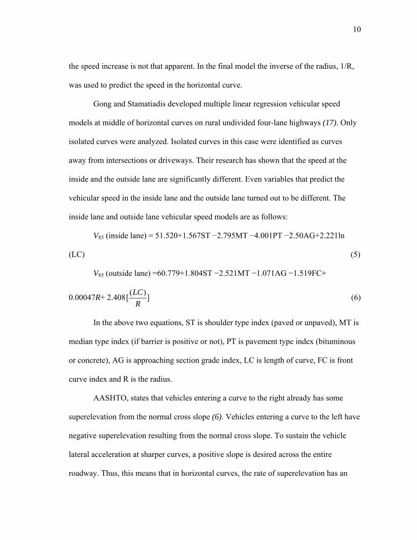
Gong and Stamatiadis developed multiple linear regression vehicular speed

models at middle of horizontal curves on rural undivided four-lane highways (17). Only

isolated curves were analyzed. Isolated curves in this case were identified as curves

away from intersections or driveways. Their research has shown that the speed at the

inside and the outside lane are significantly different. Even variables that predict the

vehicular speed in the inside lane and the outside lane turned out to be different. The

inside lane and outside lane vehicular speed models are as follows:

V85 (inside lane) = 51.520+1.567ST −2.795MT −4.001PT −2.50AG+2.221ln

(LC) (5)

V85 (outside lane) =60.779+1.804ST −2.521MT −1.071AG −1.519FC+

0.00047R+ 2.408 ])([R

LC (6)

In the above two equations, ST is shoulder type index (paved or unpaved), MT is

median type index (if barrier is positive or not), PT is pavement type index (bituminous

or concrete), AG is approaching section grade index, LC is length of curve, FC is front

curve index and R is the radius.

AASHTO, states that vehicles entering a curve to the right already has some

superelevation from the normal cross slope (6). Vehicles entering a curve to the left have

negative superelevation resulting from the normal cross slope. To sustain the vehicle

lateral acceleration at sharper curves, a positive slope is desired across the entire

roadway. Thus, this means that in horizontal curves, the rate of superelevation has an

11

impact on vehicle speed and vehicle lateral placement. Exhibit 3-15, in AASHTO

provides minimum radius for five different types of superelevation, which are 4, 6, 8, 10

and 12 percent. The two things that this exhibit suggests are that the design speed

decreases as the radius of the curve decreases and the design speed increases as the

superelevation of the curve increases. AASHTO also mentions that vehicle speeds are

affected when grades are above 5 percent (6).

A research study conducted by FHWA researchers investigated operating speed

for horizontal curves, vertical curves and tangent sections. For passenger cars in

horizontal curves the independent variable in the regression equation was 1/radius of the

curve. When the radius of a curve is 800 meter (2625 feet) or more vehicle speeds were

very similar to speeds on the tangent sections and in this situation the grade controls the

speed of the vehicle rather than the radius (2). Operating speeds decreases sharply when

the radius is 250 meter (820 feet) or less. Thus, this study also showed horizontal curve

speed was dependent on radius.

Research was done in northern Iraq to construct linear regression models at rural

horizontal curves (18). Speed data was collected at 48 curves under free flow conditions.

Speed data was collected under daylight, off-peak and dry weather conditions. The range

of radius used was from 164 feet (50 meter) to 1640 feet (500 meter), lane width from

9.8 feet (3.0 meter) to 12.1 feet (3.7 meter), shoulder width from 4.9 feet (1.5 meter) to

9.8 feet (3.0 meter), superelevation from 2-6 percent and grades from -9.3 percent to 9.3

percent. In the speed versus radius curve it was observed that speed of a vehicle along

the curve increases as the radius increases. To analyze the combined effect of curve

12

radius and grades on the curve speed, the grades were separated into four groups. Results

suggest that for radius smaller than 656 feet (200 meter), the vehicle speed is more

influenced by the radius but when the radius is more than 656 feet (200 meter), the speed

of vehicle at the curve is more influenced by the grade. The linear regression speed

model that was developed is:

V85 Curve = 17.749 + 0.5 V85 Approach + 0.05203R – 0.161 Δ + 1.416e (7)

The variables used in the above equation are, 85th percentile approach speed

(V85), radius (R) in meters; deflection angle (Δ) in degrees and superelevation (e) in

percentage. The vehicle speed in the above equation is given in kilometer per hour.

Dietz et al. reviewed eleven vehicle speed prediction models for rural horizontal

curves developed by Engineers from different countries in their Road Geometry, Driving

Behaviour and Road Safety study (19). Most of these models only used radius in their

prediction model. In addition with the radius, Biedermann (1984) and Lippold (1997)

used road width in their model while Krammes et al. (1993) included curve length and

the degree of curvature with the radius. It was observed that for radii greater than 476

feet (145 meter) the variability in the eleven speed models is less than the variability for

radii less than 476 feet (145 meter).

Kupke (1977) found that vehicle speed decreases in small curves with increasing

degree of curvature. This research mentions that due to advancements in vehicle engines,

the influence of grade is unimportant in determining vehicle speed. In previous times,

grades in excess of 2 percent had an impact but nowadays grades above 6 percent

influence vehicle speed. The impact of curvature change rate (CCR) on vehicle speed at

13

curves has mixed results. Biedermann (1984) was able to find a small influence of CCR

on speed while models developed by Koppel/Bock (1979) and Lippold (1995)

demonstrated that as the curve change rate increases, the velocity decreases.

A study in Australia finds that speeding is one of the leading factors for vehicle

accidents (20). This study also reports that the usage of advisory speed limit before

curves and police enforcement has been found to be successful in reducing the number

and severity of accidents. In addition, it states that vehicles travel slower on narrower

roads but on the other hand, crash rate increases as the lane width decreases. Here, the

method that was sought to decrease the vehicle speed was to perceptually narrow the

width of the roadway. This can be done by widening the center line and the edgeline or

by widening the center line and moving the edgeline closer to the centerline. Findings

from this research states that on narrower roads the driver mental work loads increases.

This is because on narrower roads the driver’s steering effort increases. The study states,

“Steering deviations were larger, and lateral deviations were smaller” (20). This resulted

in the vehicle to reduce their speed.

Another study was conducted in Australia to investigate vehicle speed at

horizontal curves (21). The regression analysis concluded that vehicle speed is

influenced significantly by the desired speed related to the road section and curve. Based

on the regression analysis a family of speed prediction relations was then developed. The

prediction model used radius as the sole variable to predict the vehicle speed.

The ‘Meta-Analysis’ conducted by Driel et. al. focused on the effect of edgeline,

shoulder width and road environment on vehicle speed and lateral placement. Data for

14

this study was collected in the Netherlands and in America. It was found that for both the

countries edgeline with shoulders and with or without centerline has an impact on the

vehicle speed (22). An increase in speed is found when an edgeline is added to a road

without centerline. The researchers in this study also proposed that ambient lighting

conditions (day/night), traffic volume or presence or absence of opposing traffic or

traffic on the same lane does not pose any impact on the vehicle lateral speed but due to

limited data this cannot be verified.

NIGHTTIME DRIVING

Driving on a road during the daytime and nighttime can be very different. The

absence of the sunlight makes driving very different at night than during the day. Three

things that make driving at nighttime dangerous are visibility, fatigue and alcohol (4). In

addition, 90 percent of a driver’s reaction depends on vision which is limited at

nighttime, making it harder to drive at nighttime compared to daytime (23). Some of the

reference points that people use during the day to guide them through the road are no

longer visible at night. A person’s peripheral vision, color recognition and depth of

vision at night are reduced, making it hard to focus on an object (9, 22). Ward and

Wilde, in their research states that, “Visual acuity, stimulus identification and distance

estimation, area of eye scanning and viewing distance, as well as colour and contrast

sensitivity are degraded in darkness” (24). On rural roads, where there are usually no

street lights, a driver solely depends on his/her vehicle headlights. Thus, it is very

important to check if the headlights are working properly and clean. Vision of a person

15

declines with age this makes it harder for older drivers to drive in the dark (4). The

visibility of a driver at night is also degraded from glares from oncoming vehicles (5, 9,

13, 23, 24).

Fatality rates based on speed at nighttime were about three to four times higher at

night than during the day (5, 23). A study done in New Zealand states that the chance of

getting involved in a crash in terms of distance traveled is higher at night than day (5).

This study also found that, besides visibility, fatigue and alcohol, another factor that is

related to crashes at night is that drivers do not adjust their speed to compensate for the

limited visibility at night. Drivers often overdrive their headlights at night, which means

that they drive so fast that they cannot stop within the area that is illuminated by their

headlights.

Bonneson et al. in their study showed that average nighttime speed tends to be

slower for both passenger car and truck drivers compared to average daytime speed (14).

For passenger cars the nighttime speed was 2mph slower than daytime passenger car

speeds and for trucks the nighttime speed was 1mph slower than the daytime truck

speed.

In many states, speed limit is based on the 85th percentile speed measured at

optimal conditions for free flowing vehicles during the day. Thus, it can be seen that

usually speed limit is based on daytime traffic only. Nighttime is considered as a

hazardous condition. Thus, vehicles should be driving 5-10 miles below the posted speed

limit at night (9). This is why Texas lowered their nighttime posted speed limit by 5 mph

on rural highways and farm-to-market or ranch-to-market road if the day time posted

16

speed limit was 60 mph or above (25). This allowed drivers to have more reaction time if

they needed to slow down for some reason.

RETROREFLECTIVITY

As stated earlier, retroreflectivity is the ability of a surface to reflect light back to

its source. Wider pavement markings are helpful during the daytime. At nighttime both

the width of the pavement marking as well as the amount of retroreflectivity of the

pavement marking are important. A driver will probably drive differently at night on an

8 inch wide pavement marking with low retroreflectivity compared to a 4 inch wide

pavement marking with high retroreflectivity. The Manual on Uniform Traffic Control

Devices (MUTCD), “Markings that must be visible at night shall be retroreflective

unless ambient illumination assures that the markings are adequately visible” (26). Since

rural highways are usually not illuminated, retroreflective pavement markings are used.

Retroreflectivity is measured in units of mcd/m2/lx. The MUTCD states that a

pavement marking that must be visible at night has to be retroreflective but it does not

specify the level of reflectivity. Various research studies have been conducted to

determine the minimum retroreflectivity level that is needed for drivers to view the road

at night with ease. The minimum retroreflectivity level for pavement markings that were

determined by the American Traffic Safety Services Association (ATSSA) in 2004 was

100 mcd/m2/lx for speed limit less than or equal to 50 mph and 125 mcd/m2/lx for speed

limit greater than or equal to 55 mph (10). The minimum retroreflectivity levels

specified by FHWA for different speeds are given in the following table. FHWA

17

requires the level to be 100 mcd/m2/lx for high speed, 85 mcd/m2/lx for moderate speed

and 70 mcd/m2/lx for low speed roadways (10).

Research was conducted to investigate the retroreflectivity level that drivers

preferred for nighttime driving (11). This research found that, 98 percent of the drivers

felt that a level of 94 mcd/m2/lx was adequate or more than adequate. The subjects of

this research were mostly young and research was done in ideal field conditions (11).

Thus, it is highly probable that for older drivers and non ideal conditions such as rain or

snow, the retroreflectivity level would need to be higher.

A research was designed by Aktan et. al. to determine the minimum

retroreflectivity of pavement markings for roadways with and without RRPMs (9). For

fully marked roadways (with centerline, lane lines and edgelines) without RRPMs,

different retroreflectivity levels have been recommended for different speeds. For speeds

equal to and less than 50 mph, a retroreflectivity level of 40 mcd/m2/lx, for speeds

between 55-65 mph a level of 60 mcd/m2/lx and for speeds equal to and greater than 70

mph a retroreflectivity level of 90 mcd/m2/lx has been recommended. It has also been

suggested that drivers older than 62 years may require greater retroreflectivity level than

the minimum levels determined.

Driving is influenced on a lot of factors such as roadway geometry, light

condition, weather, traffic conditions and driver’s personal characteristics. During the

day several visual clues exists that helps the driver guide their way on the road but at

night driver’s have to heavily rely on the pavement markings, markers and traffic signs.

A research was performed in a rural section of Pennsylvania were a group of drivers of

18

different age and gender were asked to drive along horizontal curves with different radii

and different retroreflectivity of the pavement markings. One of the treatments had no

pavement marking at all and the others had edgelines and centerlines with different

levels of retroreflectivity and some of the edgelines were raised retroreflective pavement

markings. After driving through the curve the drivers had to rate the curve on how well

they were able to drive through it. Results indicate that driver’s rated the curve with any

treatment better than the curve without any treatment at all. One of the findings was that

the retroreflectivity of sharp curves has more impact on drivers than on flatter curves

(10).

A low retroreflectivity level may increase the number of crashes as drivers are

not able to visualize the roadway clearly. However, a too high retroreflectivity level may

not be safe too as drivers may feel too comfortable during nighttime and drive at an

unsafe speed (8). This study on Permanent Raised Pavement Markings (PRPM)

concludes that PRPMs are less effective on two lane rural highways with low volume

traffic because drivers tend to increase their speed. In addition, this study found that

sharp curves with a degree of curvature great than 3.5 may cause an increase in

nighttime crash rate on rural, two-lane roadways.

FREE FLOWING VEHICLES

Platoon vehicles can be defined as those vehicles whose speed are influenced by

the vehicles in front of them while free flowing vehicles are those vehicles where the

19

drivers can choose their own travel speed or are vehicles that are free from interactions

in the traffic stream (27).

A study was done by Brewer and Pesti on different vehicle headway. Speed and

headway data were collected at three different points on a construction zone on I-20 in

Texas. The construction work required closing one of the two lanes. The first point was

located 1 mile upstream of the construction zone where the speed limit was 70 mph. The

second point was at the lane closure taper and the third point was at approximately at the

middle of the work zone. This single lane section was 8 mile long, with no passing zones

and the vehicle speed limit was 60 mph. After collecting the headway and speed data for

three days, researchers have found that for location 1, the headway for free flowing

vehicles was four seconds, while for location 2 and 3 the headway for free flowing

vehicles are 10 seconds and 14 seconds respectively.

In the above study it can be observed that for special conditions such as in work

zone conditions vehicles tend to keep a larger headway to stay uninfluenced from the

vehicle ahead of them while at normal conditions vehicles can pick their own speed even

at smaller headways. The above study mentions that, “A common rule of thumb is to set

a time headway threshold and consider only those vehicles that have headways greater

than or equal to the preset threshold” (28).

Research was also conducted at Montana State University to determine the free

flowing vehicles on rural highways. Data were collected on rural two-lane and four–lane

highways. To determine the free flow or car following interactions, the relationship

between speed and time headway were established. After the time headway exceeded a

20

certain threshold, the number of vehicles following diminished. These vehicles were

considered as free flowing vehicles. Data from this research concludes that free flowing

vehicles on two lane rural highways are defined as vehicles having headway of six

seconds or greater (27).

When developing vehicle speed model, researchers tend to include only free flow

vehicles. The threshold that researchers use to define free flow vehicles varies from four

to six seconds. Gong and Stamatiadis used five seconds as the threshold for free flow

vehicles (17). Medina and Tarko also used five seconds to classify between free flow

and platoon vehicles (15).

TEXAS CURVE ADVISORY SPEED SOFTWARE

TTI researchers, Bonneson et al., developed software called, Texas Curve

Advisory Speed Software (TCAS) to automate the procedure and guidelines to

determine the advisory speed for horizontal curves (29). In addition to determining the

advisory speed, this software provided the side friction demand for the curves which

were then used to set the severity levels. Based on the severity levels, guidelines were

provided on what type of warning signs and other delineation treatments should be used

for that particular curve.

Using vehicle speed models for horizontal curves, Bonneson et al. developed this

software. The first model that was developed was as follows:

21

[ ]t

p

xtkttpc V

bR

eIbIbVbVbbRV ≤

⎟⎟⎟

⎠

⎞

⎜⎜⎜

⎝

⎛

+

++++−=

5.0

2

432

210

0322.01100)47.1(001.0)47.1(0.15

(8)

With,

)5.0(10.3

cp ICos

RR−

+=

In the above equation,

Vc = curve speed, mph

Vt = tangent speed, mph

Rp = travel radius path, feet

b3 = calibration coefficient for trucks

Itk = indicator variable for trucks (=1.0 if model is used to predict truck speed, 0.0

otherwise)

b4 = calibration coefficient for other factors

Ix = indicator variable (=1.0 if factor is present, 0.0 otherwise)

e = superelevation rate, percent, and

Ic = curve deflection angle, degrees (14)

After performing regression analysis, calibration coefficients were developed

yielding the following model to predict the 85th percentile vehicle speed at curves for the

TCAS software (14):

22

85,

5.0285,85,

85, 00109.011000150.0000073.000106.0196.0(0.15

tp

tkttpc V

R

eIVVRV ≤

⎟⎟⎟

⎠

⎞

⎜⎜⎜

⎝

⎛

+

+−+−=

(9)

Here,

Vc,85 = 85th percentile curve speed, mph and

Vt,85 = 85th percentile tangent speed, mph

The side friction demand increase also known as the frictional differential was

used to determine the severity level because the increase in side friction that a driver

accepts is proportional to the energy required to slow the vehicle to the curve speed.

Frictional differential is the difference between the side friction factor incurred by the

vehicle and the upper limit of comfortable friction. Using the calibration coefficients

from the above equation, the frictional differential equation that was developed for the

TCAS software is:

onDemandSideFrictiIVVf vct =−=Δ )(000073.0 285,

285, (10)


∆f=friction differential and

Iv=indicator variable (=1.0 if Vt,85>Vc,85; 0.0 otherwise)

This software was implemented as a excel spreadsheet. The advisory speed could

be determined by two different processes. One is by, “Known Curve Geometry” and the

other is the “Survey of Curve”. “Known Curve Geometry” is used when geometric data

information about the roadway is known from the actual design of the roadway while

23

“Survey of Curve” is used when geometric data information is obtained by surveying the

roadway. The top one-third cells in this software contain the ‘input data’ cells. The

calculation cells are located in the bottom two-thirds of the worksheet. The radius is

calculated from the deflection angle and the curve length while the ball bank reading is

used to calculate the superelevation. The bottom third of the spreadsheet provides the

traffic control device guidance based on the advisory speed that is calculated. The third

row in this section provides the curve severity category which is based on the side

friction demand increase thresholds. This software divides the severity of a curve into

five levels.

VEHICLE SPEED DATA COLLECTION METHODS

Sun, Park, Tekell and Ludington evaluated edgeline pavement markings on

narrow roads in Louisiana using vehicle speed and lateral placement data. Road Tubes

also known as airswitch devices were used to collect the vehicle speed and lateral

placement data. The researchers stated that this method was more reliable, less intrusive

and easier to set up while compared to other vehicle speed and lateral placement data

collection methods (30). Using three sensors with eight tubes, the data that were

collected for this study are: (a) number of right tires touching the 1-feet section of

roadway next to the pavement edge, (b) number of right tires touching the roadway

section between 1 and 2 feet from the edgeline, (c) number of vehicles crossing the

centerline, (d) hourly traffic volume by direction, and (e) operation speed.

24

Traffic engineers have also used Global Positioning Systems (GPS) as an

alternative method to collect traffic data (31). The purpose of this study was to collect a

vehicle speed profile, vehicle acceleration and deceleration, vehicle queue length and

vehicle’s positions at highway work zones in Indiana. GPS was used on a test vehicle to

collect these data at a work zone. The vehicle speed and position data is recognized by

satellite signals and recorded this device. At each data point it records the vehicles

position, speed time and the distance between the current and last time points. As the test

vehicle is traveling with other traffic on the road, the GPS not only gives a speed profile

of the test vehicle but also of the traffic flow (31).

LINEAR MIXED MODELS

While making a model one has to characterize the dependence of a response

variable on one or more covariates. These variables can be fixed or random. A statistical

model that contains both fixed and random variable is known as mixed-effects model

(32). When the parameters in a mixed-effects model are chosen to be linear, the model

then is known as linear mixed model. Statistical software packages such as CRAN-R and

SPSS are capable of modeling linear mixed models. Generalized linear models do not

address correlated errors. “The Linear Mixed Models procedure expands the general

linear model so that the error terms and random effects are permitted to exhibit

correlated and non-constant variability. The linear mixed model, therefore, provides the

flexibility to model not only the mean of a response variable, but its covariance structure

25

as well” (33). In the CRAN-R manual, Fox, in his Linear Mixed Model chapter gives the

Laird-Ware form of the linear mixed model, which is:

yij = β1x1ij + … + βpxpij + bi1z1ij + … + biqzqij + εij (11)

Here,

• yij: the response variable.

• β1……. βp: the fixed – effect coefficients.

• x1ij…….xpij: the fixed – effect regressors.

• bi1…….. bip: the random – effect coefficients.

• z1ij………zqij: the random – effect regressors.

• εij: the error for observation j in group i.

SUMMARY

While developing vehicle speed models for the midpoint of horizontal curves,

researchers have used many different variables. Some of the most common used

variables are tangent speed, approach speed, radius, deflection angle, curve length and

lane width. One observation that all researchers made was that vehicle speed increases

with the increase in the curve radius. Another important observation is that for sharper

curves vehicle speed is influenced more by the curve characteristics while for flatter

curves the vehicle speed is impacted more by the cross sectional characteristics of the

roadway such as lane width and shoulder width. Another important aspect of developing

a vehicle speed model is to use free flowing vehicles. Researchers use between 4-6

seconds to distinguish between free flowing and platoon vehicles.

26

Nighttime driving is very different from daytime driving due to the absence of

the sun at night. Visibility of the roadway is significantly reduced at nighttime especially

if there is no street lighting. The fatality rate per mileage driven at night is higher

compared to day. Visibility, fatigue and alcohol are three reasons for the high fatality

rate at night. Visibility is an important factor while driving at night but unfortunately

many drivers do not adjust their speed accordingly due to the limitations caused by

visibility at night. Due to the high crash rate during nighttime, the state of Texas has a

lower speed limit at night for high speed roadways. Thus, vehicle speed at day time and

nighttime does vary.

Retroreflective materials are easier to see at night as they bounce of light to the

light source. This is why MUTCD requires all pavement markings that are to be used at

night to be retroreflective. Even though, MUTCD requires pavement markings to be

retroreflective it does not provide any minimum level of retroreflectivity that should be

used. Different studies have shown that the minimum retroreflectivity level that is

needed for drivers to feel comfortable is around 100 mcd/m2/lx. As too low

retroreflectivity is not safe because drivers are not able to view the road properly, too

high of a retroreflectivity may not be safe too as drivers may feel too comfortable

leading them to speed and even over run their headlights.

By inputting the data for radius, curve length, superelevation, deflection angle

and tangent speed the TCAS software is able to determine the advisory speed and also

the severity level of the curve. Multiple linear regression speed model was used to

27

develop this model. Other researchers also use multiple linear regression models to

develop vehicle speed models.

Vehicle speed at day and night is different at tangent sections and also curve

sections of roadways. As retroreflectivity of the pavement markings determines how

clearly a driver is able to view the road, retroreflectivity is an important factor in driving

at night because the driver may choose their speed depending on how clearly they can

view the road. Thus, it is important to see how speed changes at day and night for curves

with different geometric characteristics and retroreflectivity levels.

28

3. BACKGROUND INFORMATION ON DATA

Vehicle speed and vehicle lateral placement data on 18 two-lane two-way

horizontal curves near Nashville, Tennessee were collected in the outside lane by the

Texas Transportation Institute (TTI) during summer of 2007. This dataset was used for

the analysis. The dataset is described below:

• Data were collected along 18 rural two-lane, two-way horizontal curves which

differ from each other in terms of its geometric characteristics such as shoulder

width, lane width, edgeline retroreflectivity, superelevation, grade, radius of the

curve, curve length, deflection angle, speed limit and advisory speed.

• Data were collected at each curve for at least a 48 hour period during weekdays.

• To measure the vehicle speed and lateral placement, speed traps were placed at four

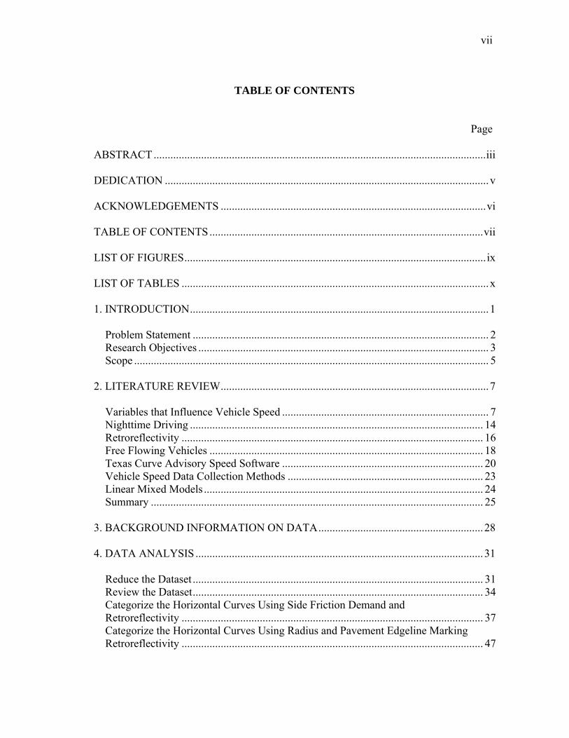
locations in the outside lane of each curve as illustrated in Figure 1 and described

below:

Upstream Location (U) – This point was located far enough upstream so that the

vehicle speeds were be affected by the curve or even the warning signs. It was

approximately 1000 feet upstream of the curve warning sign.

Advance Curve Warning Sign Location (W) – This was the location of the

advance curve warning sign or the location where the sign would have been

located if there was no sign present.

Point-of-Curve Location (PC) – This point was located at the point-of-curvature

(PC) of the horizontal curve.

29

Midpoint-of-Curve Location (MC) – This point was located at the midpoint of

the horizontal curve (MC).

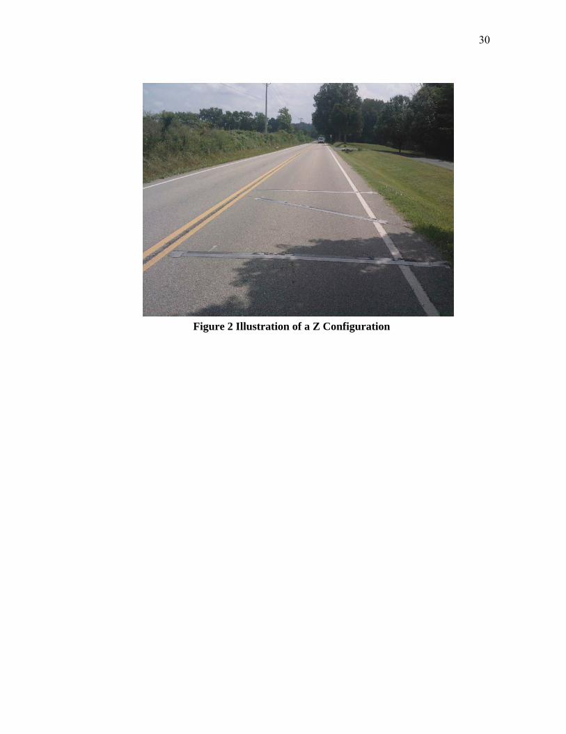
Figure 1 Location of the Traffic Classifier

• Each vehicle was tracked through all four points so the author could relate the

speed at the MC to any other points if needed during the analysis.

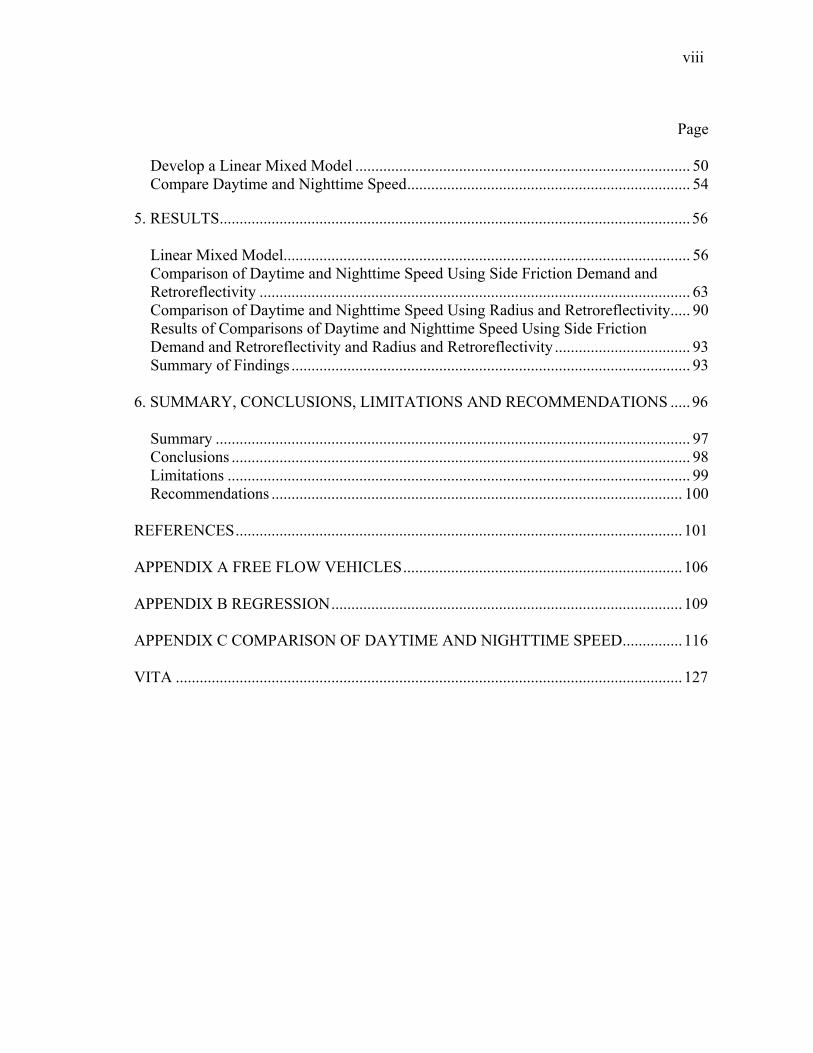
• JAMAR traffic classifiers in conjunction with piezoelectric road sensors were

placed in a Z configuration as shown in Figure 1 to collect the vehicle speed and

lateral placement data. Figure 2 on the next page illustrates the Z configuration that

was placed on one of the locations.

30

Figure 2 Illustration of a Z Configuration

31

4. DATA ANALYSIS

In this section, the author focuses on the procedure used to reduce the dataset

prior to the analysis. The author describes the variables that were used as an input in the

TCAS software to determine the side friction demand of the horizontal curves and how

the curves were categorized. The author also outlines his statistical methodology used to

create the linear mixed model and the statistical methodology used to compare the

daytime and nighttime speed data.

REDUCE THE DATASET

The steps that were taken to reduce the dataset area as follows:

Step 1

The first step in reducing this dataset was to exclude erroneous and missing data.

Step 2

The second step in this reduction process was to eliminate extraneous data. As

stated above, the original dataset has vehicle speed information at four points along the

curve. However, for this study only the speed at the midpoint of the curve or speed at

MC was used because it is assumed that this is the point where drivers reach their

minimum speed along the curve. In addition, when developing vehicle speed models on

horizontal curves, generally the models are based on operating speeds at the midpoint of

the curves (14, 15, 16, 17, 18, 21). Thus, the speeds at PC, W and U were excluded from

the dataset.

32

The curve geometry data has information on shoulder width, lane width, edgeline

retroreflectivity, superelevation, grade, radius of the curve, deflection angle, speed limit

lane width and advisory speed for each of the curves. From this dataset, data for only the

radius of the curve, deflection angle, curve length, speed limit and retroreflectivity level

were kept for the analysis. A description of these variables is given in the Review the

Dataset section on page 32.

Step 3

The third step in reducing this dataset was to exclude vehicles that traveled

through the curve half an hour before and after the sunset and sunrise. In addition, in this

step, rain data was eliminated too.

Step 4

Only isolated free flowing vehicles were included in the analysis. Isolated and

free flow vehicle is defined as those vehicles whose speed will not be influenced by the

vehicle in front of the vehicle of interest. Speed profile was plotted for different

headways starting from 1 second and increasing the increment by 1 second. This was

done for the curves with high volumes because it is easier to observe the noise in the

data with high volume traffic compared to low volume traffic. This speed profile is a

graph of vehicle n against vehicle n+1 at the midpoint of the graph. Here n is the vehicle

of interest. If the data from the graph shows that, the slope of the regression line is equal

to y = x or close to that then the vehicles are defined as platoon vehicles but if the graph

demonstrates that the data is scattered, this will suggest that the vehicles are isolated. In

33

other words, if the slope is one then it will mean that the vehicle of interest is

maintaining the speed of the vehicle that is in front of it. However, if the slope is not

close to the y = x line then the vehicles are choosing their own speed. The first headway

that shows a graph with scattered data was considered as the minimum headway required

for isolated vehicles. Vehicles that have headway less than this minimum headway were

excluded from the analysis. After plotting the speed of vehicles at some of the curves

that were used in this analysis, it was determined that free flowing vehicles had an

approximate headway of 6 seconds.

Curve 15 was one of the high volume curves. Appendix A has the speed profile

plots for curve 15 for headways 1 through 6. These plots include a linear trend line with

an R squared value of the trend line. An R squared value close to 1 will determine that

the vehicles are in platoon. Smaller R squared values will determine that the vehicles are

in free flowing condition. The linear trend line has been plotted by fixing the intercept to

0 so that it mimics a y = x graph. From these plots it was observed that free flowing

vehicles in this curve occur for headways 5 second and larger.

To be conservative, the author defined free flowing vehicles as having headway

of 7 seconds or more for this analysis. In this step vehicle that has headways less than 7

seconds were excluded.

Step 5

Here the plan was to remove vehicles that that have the presence of opposing

traffic while going through the curve. This is why the time that a vehicle was present at

the opposite direction was measured but due to the uneven time drifts in the sensors it

34

was difficult to determine the exact time an opposing vehicle was present. Thus,

unfortunately for this analysis, vehicle with and without the influence of opposing traffic

were included in the analysis.

Step 6

The data were collected in such a way so that the number of axles of each vehicle

passing through the curve could be calculated. This step consisted of determining the

percentage of each type of vehicle and determining whether speeds differ among

different types of vehicles (car vs. truck). However, when tracking the vehicles along the

curve at the four locations (U, W, PC and MC) the data revealed that a same vehicle

would have different number of axles at different locations. Due to this technical

difficulty, the idea of determining the types of vehicles was abandoned.

REVIEW THE DATASET

In this section, the procedures that were used to collect the data for the variables

that were used as input data in the TCAS software for the analysis is reviewed.

Furthermore, how these variables were used in the analysis is discussed as well.

Vehicle Speed at Points MC

A speed trap was placed using JAMAR traffic classifiers in conjunction with

piezoelectric road sensors to measure the speed at MC. The traffic classifier provides the

time stamps when a vehicle crosses over the sensors. With these time stamp data and

simple geometry the vehicle speed and lateral placement was calculated. Even though

35

this is not one of the methods that has been identified in the Identify Methods to Collect

Vehicle Speed and Vehicle Lateral Placement Data section, this data is reliable, as many

of the researchers at TTI use this method to collect vehicle speed and lateral placement

data.

Prior to performing the analysis, erroneous data, and rain data were excluded

from the dataset.

Edgeline Retroreflectivity at MC

Retroreflectivity level was measured with a handheld pavement marking retro

reflectometer. The average of four readings of retroreflectivity level was used to

determine the retroreflectivity level at MC.

Superelevation at MC

Superelevation was measured using a ball-bank reading indicator. This was used

as input data for the TCAS software.

Radius of the Curve

Radii of the horizontal curves were measured by a radiusmeter. This value was

checked by measuring the radius on an aerial map.

Deflection Angle

Deflection angle was measured in the direction of travel by calculating the

difference in the approach tangent heading and the exiting tangent heading. This was

used as an input for the TCAS software.

36

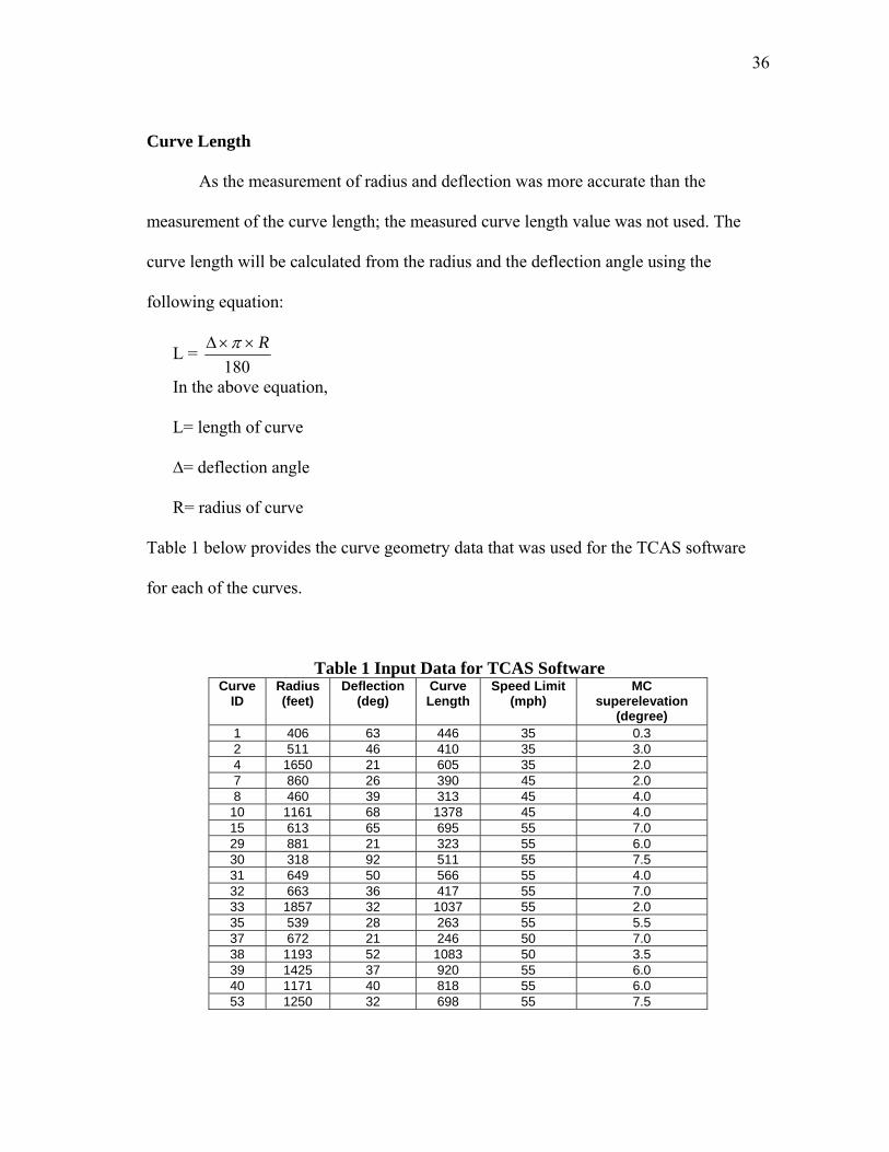
Curve Length

As the measurement of radius and deflection was more accurate than the

measurement of the curve length; the measured curve length value was not used. The

curve length will be calculated from the radius and the deflection angle using the

following equation:

L = 180

R××Δ π


L= length of curve

∆= deflection angle

R= radius of curve

Table 1 below provides the curve geometry data that was used for the TCAS software

for each of the curves.

Table 1 Input Data for TCAS Software Curve

ID Radius (feet)

Deflection (deg)

Curve Length

Speed Limit (mph)

MC superelevation

(degree) 1 406 63 446 35 0.3 2 511 46 410 35 3.0 4 1650 21 605 35 2.0 7 860 26 390 45 2.0 8 460 39 313 45 4.0

10 1161 68 1378 45 4.0 15 613 65 695 55 7.0 29 881 21 323 55 6.0 30 318 92 511 55 7.5 31 649 50 566 55 4.0 32 663 36 417 55 7.0 33 1857 32 1037 55 2.0 35 539 28 263 55 5.5 37 672 21 246 50 7.0 38 1193 52 1083 50 3.5 39 1425 37 920 55 6.0 40 1171 40 818 55 6.0 53 1250 32 698 55 7.5

37

CATEGORIZE THE HORIZONTAL CURVES USING SIDE FRICTION

DEMAND AND RETROREFLECTIVITY

One of the objectives of this study was to compare the daytime and nighttime

speed of vehicles at the midpoint of the curve. To perform this analysis, the curves were

categorized using different methods. In each method, the curves were categorized

according to its respective side friction demand and retroreflectivity level. Side friction

demand was used because, “The increase in side friction demand that a driver accepts is

proportional to the energy required to slow the vehicle to the curve speed” (14). As

stated earlier, the TCAS software was used to determine the side friction demand. From

the overview of the TCAS software in the Literature Review section, it was observed

that one other advantage of using side friction demand is that the side friction demand

equation includes the radius, curve deflection angle and superelevation of the curve.

Thus, there will be no need to categorize the curves separately in terms of the radius,

curve deflection angle and superelevation.

As stated in the Literature Review section, in addition, to providing the side

friction demand value, the TCAS software also categorizes the curves into five groups

according to the side friction demand value. The author did not use the same threshold

values used in the TCAS software to categorize the curves but used those thresholds as

guidelines when he categorized the curves for this analysis.

The first reason was because for this analysis, the curves were not grouped based

only on the side friction demand value but also according to the retroreflectivity value.

Dividing the curves into five groups based just on side friction demand would increase

38

the total number of groups being analyzed. As this analysis has only 18 curves, making

too many groups could become an issue as some groups may not have any curves while

others may have too few curves to analyze and to come up with a conclusion. The

second reason was that the threshold values used in the TCAS software is used as a

guideline to determine the type of warning treatment needed for a curve. However, that

is not the scope of this study. Thus, it is not necessary to use the threshold values used in

the TCAS software.

Retroreflectivity level was used as the other factor in categorizing the curves as

one of the objectives was to determine at what retroreflectivity levels the daytime speed

and nighttime speeds significantly differ.

The author decided to categorize side friction demand and retroreflectivity into 2-

3 separate groups. However, it was determined that some curves could fall into more

than one group if the threshold between each group is changed. This led the author to

categorize the curves in six different methods. Categorizing the curves into six different

methods would determine the sensitivity of the curves. In other words, by changing the

threshold points between the groups, the author replaced curves from one group to

another group to examine how this replacement of curves changed the daytime and

nighttime speed within a group and how the speeds are changing among different

groups. The matrix in Table 2 Curve Categorization Matrix demonstrates in what group

the curves belong to for the six methods. In addition, the matrix also provides the side

friction demand obtained from the TCAS software and, the retroreflectivity level for

39

each curve. Definitions of the groups and explanations on how the curves were grouped

for the six methods are given below:

Table 2 Curve Categorization Matrix Using Side Friction Demand and

Retroreflectivity

Curve ID

Side Friction Demand Increase

Marking Retroreflectivity

(mcd/m2/lx)

Method

1 2 3 4 5 6 1 0.07 157 C C B C E 2 0.04 286 B B A B B C 4 0.00 384 A A A B B C 7 0.03 90 B B A A A A 8 0.07 117 C C B C C D 10 0.00 285 A A A B B C 15 0.07 175 C C B C E 29 0.02 201 B B A B B 30 0.12 222 C 31 0.08 117 C C B C C D 32 0.06 160 C C B C E 33 0.00 153 A A A A B 35 0.08 129 C C B C C D 37 0.02 203 B B A B B 38 0.01 479 B B A B B C 39 0.00 101 A A A A A A 40 0.00 119 A A A A A A 53 0.00 300 A A A B B C

Method 1

In this method the curves was categorized into groups based on its side friction

demand value only; the effects of retroreflectivity level was not analyzed in this method.

As can be seen from the above table, in this method there are three groups, which are as

follows:

40

• Group A: Curves with side friction demand value of 0 • Group B: Curves with side friction demand greater than 0 and less than

0.05 • Group C: Curves with side friction demand greater than 0.05

From the Literature Review section of Development of Guidelines for

Establishing Effective Curve Advisory Speeds, it was found that curve warning signs are

not needed when the friction differential is 0.00. This means that a vehicle may not need

a slower speed than the tangent section speed as they go through a curve when the

frictional differential is 0.00. Thus, it is assumed that visibility of the roadway will not

be an issue at these curves especially at night. As a result, the day and night time speed

may not be significantly different in this group. To test this assumption, Group A was

created.

The author chose 0.05 as the side friction threshold value between Group B and

Group C because after observing the side friction values of the 18 curves the author

identified that there was one curve with side friction value of 0.04 and one curve with

side friction value of 0.06 but there was no curve with a value of 0.05. Hence, 0.05 was

used as the threshold between Group B and Group C as no curve has a side friction value

of 0.05

If Group C is observed, then one will find that there are seven curves in this

group. Out of these seven curves, six of them have side friction values between 0.06 and

0.08 while the other one, Curve 30, has a side friction demand value of 0.12. This is the

largest side friction value in this dataset. The difference between this largest side friction

demand value and the second largest side friction demand value is (0.12 – 0.08) = 0.04.

41

Since there are no side friction demand values between 0.12 and 0.08; having Curve 30

in Group C may provide inconclusive results. To eliminate this problem, Curve 30 could

have been put into another group which would have curves having side friction demand

value greater than 0.10. However, in that case that group would contain only Curve 30

and it maybe biased to obtain any conclusions from a group that has only one curve.

Hence, Group D was not created.

To eliminate the issue of having inconclusive results in Group C because of the

big difference between the side friction demand value of the largest side demand value

and the second largest side friction demand value, in Method 2, these same groups was

retained except that Curve 30 was eliminated from the analysis. In fact, Curve 30 was

not used in any of the other methods.

Method 2

As mentioned above, this method is exactly the same as Method 1, except that

curve 30, which has a side friction level of 0.12, was excluded here.

Method 3

This method was used as the primary step for categorizing the curves for the

latter three methods. In this method the curves were also categorized based only on the

side friction demand values. The difference between the previous two methods and this

method is that here the curves were categorized in two groups rather than three groups.

Here, Group A and Group B of Method 1 and 2 were combined into one group, which is

named as Group A and Group C of Method 1 and 2 is renamed as Group B.

42

The reason for combining Group A and Group B of the previous two methods

into one group in this method is that, in the next methods the curves were categorized

based on both the side friction demand value and retroreflectivity level. Creating three

separate groups for side friction demand and retroreflectivity level would create a 3 × 3

matrix, which means that there would be nine different combinations of side friction

demand and retroreflectivity. However, categorizing the curves into nine different

combinations of side friction demand and retroreflectivity level may lead to inconclusive

results because there may not be enough data in each group to analyze as altogether there

are only 17 curves available to analyze. Hence, to reduce the size of the matrix, in the

latter three methods, side friction demand was divided into two groups.

One can question why to make two groups, Group A and B were combined

instead of combining Group B and C of Methods 1 and 2. The reason for combining

Group A and Group B of the previous two methods is that, there are curves with side

friction demand value of 0.00 and 0.01 and 0.00 is the threshold between Group A and

Group B. On the other hand as stated previously, there are no curves with side friction

demand value of 0.05, which is why 0.05 was chosen as the threshold between Group B

and Group C. As a result, one can see that it is easier to combine Group A and B rather

than to combine Group B and C.

In the next three methods after categorizing the curves in terms of side friction

demand value using the technique used in this method, the curves were categorized

further using retroreflectivity level.

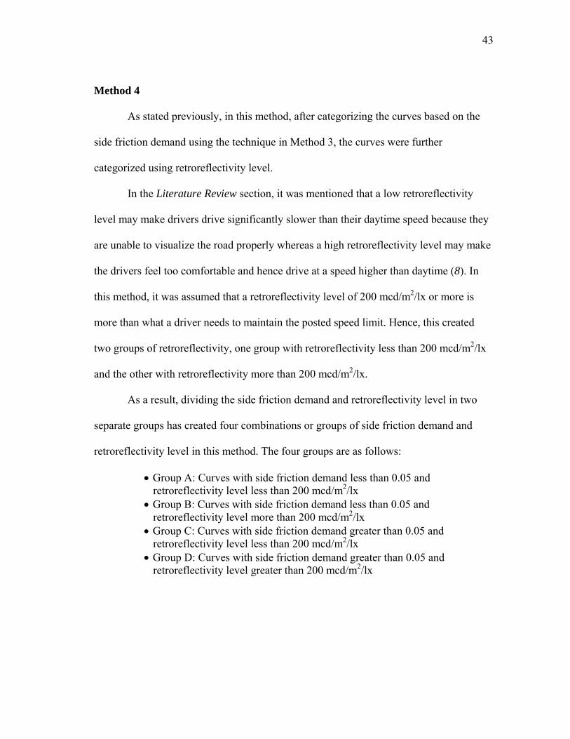
43

Method 4

As stated previously, in this method, after categorizing the curves based on the

side friction demand using the technique in Method 3, the curves were further

categorized using retroreflectivity level.

In the Literature Review section, it was mentioned that a low retroreflectivity

level may make drivers drive significantly slower than their daytime speed because they

are unable to visualize the road properly whereas a high retroreflectivity level may make

the drivers feel too comfortable and hence drive at a speed higher than daytime (8). In

this method, it was assumed that a retroreflectivity level of 200 mcd/m2/lx or more is

more than what a driver needs to maintain the posted speed limit. Hence, this created

two groups of retroreflectivity, one group with retroreflectivity less than 200 mcd/m2/lx

and the other with retroreflectivity more than 200 mcd/m2/lx.

As a result, dividing the side friction demand and retroreflectivity level in two

separate groups has created four combinations or groups of side friction demand and

retroreflectivity level in this method. The four groups are as follows:

• Group A: Curves with side friction demand less than 0.05 and retroreflectivity level less than 200 mcd/m2/lx

• Group B: Curves with side friction demand less than 0.05 and retroreflectivity level more than 200 mcd/m2/lx

• Group C: Curves with side friction demand greater than 0.05 and retroreflectivity level less than 200 mcd/m2/lx

• Group D: Curves with side friction demand greater than 0.05 and retroreflectivity level greater than 200 mcd/m2/lx

44

After categorizing the curves in its respective group the author determined that

there were no curves that met the requirements of Group D. Hence, there is going to be

only three groups for this method.

Method 5

This method was a modification of Method 4. Similar to method 4, after

categorizing the curves based on the side friction demand using the technique in Method

3, the curves here were further categorized using retroreflectivity level.

In the previous method, 200 mcd/m2/lx was used as the threshold to create the

two groups of retroreflectivity level. Here too, there were two groups of retroreflectivity

but the threshold was defined differently than in the previous method. The issue in the

previous method was that, the author realized that there are some curves such as curves

29 and 37 that have retroreflectivity value close to 200 mcd/m2/lx (201 mcd/m2/lx and

203 mcd/m2/lx respectively). Previously, it was mentioned that the retroreflectivity

values that are used here are an average of four retroreflectivity values that were

measured close to the MC location. The retroreflectivity value of curves 29 and 37 may

become less than 200 mcd/m2/lx if another reading was taken. In that case these two

curves would have been placed in Group A instead of Group B.

To resolve this issue, curves that were within ± 50 mcd/m2/lx of 200 mcd/m2/lx

were excluded from the analysis in this method. The author could have chosen a smaller

margin (i.e. ± 20 mcd/m2/lx), which would have excluded fewer curves from the

analysis. However, just to be conservative, the author chose ± 50 mcd/m2/lx as the

margin because after all the retroreflective values used in the analysis are an average

45

value and another reading may well change that average quite a bit if the next reading

location was in a spot were the retroreflectivity might have worn out significantly

compared to the other locations due to reasons such as weather, vehicle tire etc.

Hence, in this method one group has curves with retroreflectivity value less than

150 mcd/m2/lx and the other group has curves with retroreflectivity more than 250

mcd/m2/lx. Thus, due to a 2 × 2 matrix, this method too has four groups, which are as

follows:


• Group B: Curves with side friction demand less than 0.05 and retroreflectivity level more than 250 mcd/m2/lx

• Group C: Curves with side friction demand greater than 0.05 and retroreflectivity level less than 150 mcd/m2/lx

• Group D: Curves with side friction demand greater than 0.05 and retroreflectivity level greater than 250 mcd/m2/lx

It was determined that there was no curve that met the requirement of Group D.

Thus, similar to Method 4, in this method too there will be three groups.

Method 6

This method is very similar to Method 5. In the previous method, curves that

were within ± 50 mcd/m2/lx of 200 mcd/m2/lx were excluded from the analysis. In this

method, the curves that were excluded in Method 5 were included in the analysis by

creating a separate group for those curves. Thus, here, there are two groups for side

friction demand and three groups for retroreflectivity level which has created six

combinations or six groups of side friction demand and retroreflectivity level by creating

a 2 × 3 matrix. The six groups developed for this method are as follows:

46


• Group B: Curves with side friction demand less than 0.05 and retroreflectivity level greater than 150 mcd/m2/lx and less than 250 mcd/m2/lx

• Group C: Curves with side friction demand less than 0.05 and retroreflectivity level greater than 250 mcd/m2/lx

• Group D: Curves with side friction demand greater than 0.05 and retroreflectivity level less than 150 mcd/m2/lx

• Group E: Curves with side friction demand greater than 0.05 and retroreflectivity level greater than 150 mcd/m2/lx and less than 250 mcd/m2/lx

• Group F: Curves with side friction demand greater than 0.05 and retroreflectivity level greater than 250 mcd/m2/lx

Group F of this method and Group D of the previous method are the same. It was

mentioned in the previous method that no curves met the requirements of Group D

which is why Group D was omitted from the analysis. Here too, Group F was excluded

from the analysis. Thus, there are give groups of curves in this method.

By including the curves that were excluded from the analysis in Method 5, in this

method, the author intends to determine whether this new group of curves have speeds

similar to curves with retroreflectivity less than 150 mcd/m2/lx or similar to curves with

retroreflectivity more than 250 mcd/m2/lx or whether this new group of curves has speed

which are significantly different from curves less than 150 mcd/m2/lx and more than 250

mcd/m2/lx.

47

CATEGORIZE THE HORIZONTAL CURVES USING RADIUS AND

PAVEMENT EDGELINE MARKING RETROREFLECTIVITY

As mentioned in the previous section, one of the objectives of this study was to

compare the daytime and nighttime speed of vehicles at the midpoint of the curve. In the

previous section, the curves were categorized into different groups using the side friction

demand and the pavement edgeline marking retroreflectivity. All the researchers who

developed vehicle speed model in the past has used radius as an independent variable to

predict the vehicle speed at curves. This demonstrates that radius has the biggest impact

on vehicle speed.

As using side friction demand to categorize curves is not commonly used, in this

section the author grouped the curves based on the radius to determine whether the result

of the day and nighttime speed difference found using radius to classify curves into

different groups is the same as grouping the curves according to the side friction demand

value. If classifying the curves based on the radius yields similar day and nighttime

speed difference as classifying the curves based on the side friction demand then it

would mean that it is justified to group curves based on the side friction demand too.

Similar to the previous section the author would also use retroreflectivity as the other

factor to classify the curves.

To determine whether classifying the curves based on radius yields similar or

different result as classifying the side friction demand, the author repeated Method 4 and

Method 5 of the previous section but instead of using side friction demand and pavement

edgeline marking retroreflectivity, the author used radius and pavement edgeline

48

marking retroreflectivity. The matrix in Table 3 demonstrates in what group the curves

belong to for the two methods and provides the radius and pavement edgeline marking

retroreflectivity for each curve. Definitions of the groups and explanations on how the

curves were grouped for the two methods are given below:

Table 3 Curve Categorization Matrix Using Radius and Retroreflectivity Curve

ID Radius (feet)

Marking Retroreflectivity

(mcd/m2/lx)

Method

1 2

1 406 157 A 2 511 286 B B 4 1650 384 D D 7 860 90 C C 8 460 117 A A 10 1161 285 D D 15 613 175 A 29 881 201 D 30 318 222 B 31 649 117 A A 32 663 160 A 33 1857 153 C 35 539 129 A A 37 672 203 B 38 1193 479 D D 39 1425 101 C C 40 1171 119 C C 53 1250 300 D D

Method 7

This method was very similar to Method 4 of the previous section. As mentioned

earlier, instead of grouping the curves on the basis of side friction demand and

retroreflectivity level, the curves were divided based on radius and retroreflectivity. A

study sponsored by FHWA states that vehicle speed decreases sharply for radius less

than 250 meter (820 feet) (2). On the basis of this, two curve groups were created, one

49

group with curves less than 820 feet and the other group with curves less than 820 feet.

Using the logic presented in Method 4 and to keep consistency with Method 4 of the

previous section, the retroreflectivity level threshold was kept at 200 mcd/m2/lx. Hence,

the four groups in this method are:

• Group A: Curves with radius less than 820 feet and retroreflectivity level less than 200 mcd/m2/lx

• Group B: Curves with radius less than 820 feet and retroreflectivity level more than 200 mcd/m2/lx

• Group C: Curves with radius greater than 820 feet and retroreflectivity level less than 200 mcd/m2/lx

• Group D: Curves with radius greater than 820 feet and retroreflectivity level greater than 200 mcd/m2/lx

Method 8

This method was very similar to Method 5 of the previous section. Once again,

instead of using side friction demand the author used radius of the curve. Method 4 and

Method 5 of the previous section used the same side friction demand threshold value. To

keep consistency with the technique of Method 4 and Method 5 of the previous section,

the radius threshold value for this method was kept the same as Method 7 above, which

was 820 feet. In Method 5 of the previous section, curves with edgeline marking

retroreflectivity level between 150 mcd/m2/lx and 250 were excluded from the analysis.

The same thing was done here too. The four groups in this method are:

• Group A: Curves with radius less than 820 feet and retroreflectivity level less than 150 mcd/m2/lx

• Group B: Curves with radius less than 820 feet and retroreflectivity level more than 250 mcd/m2/lx

• Group C: Curves with radius greater than 820 feet and retroreflectivity level less than 150 mcd/m2/lx

50

• Group D: Curves with radius greater than 820 feet and retroreflectivity level greater than 250 mcd/m2/lx

DEVELOP A LINEAR MIXED MODEL

After categorizing the data, the first step in analyzing the data consisted of

developing a linear mixed model. Statistical models were developed in the past to find

out how certain independent variables influences a dependent variable. Several models

can be developed in this regard such as a linear model, non-linear model, mixed effects

model, generalized linear model, linear mixed model etc. Depending on the type of

research and the type of data, researchers use different models. For this analysis, a linear

mixed model was developed. The reasons for this are (1) a linear mixed model can

contain both fixed and random variables (2) it is an expansion of the generalized linear

model where the error terms and random effects can produce correlated and non-

constant variability. To simplify the statistical procedure, a linear model was chosen

over a non-linear model.

A stepwise linear regression was also conducted to develop the linear mixed

model. The advantage of creating such kind of model is that, it identifies the significant

variables and creates a model with the significant variables only. Hence, one does not

have to create multiple models with different combinations of the independent variables

to determine which variables are significant in predicting the dependent variable. The

statistical software package, SPSS was used to develop the linear mixed model as it has

the capability to conduct a stepwise linear regression. In the ‘Analyze’ menu of SPSS,

51

the ‘Stepwise’ option in ‘Linear Regression’ was used to conduct the stepwise regression

analysis.

To develop the model, the author used the independent variables (curve length,

superelevation, posted speed limit, deflection angle) that were used to calculate the

increase in side friction demand also known as the frictional differential in the TCAS

software. One reason for using those variables was because the frictional differential in

the TCAS software was calculated from a vehicle speed model and the vehicle speed

model included variables that influence vehicle speed at the midpoint of a curve.

Another reason was because the vehicle speed model that was developed for the TCAS

software is actually a modification of the traditional vehicle speed model given in

Equation 1 in the Literature Review section. Furthermore, from the Literature Review

section it can also be observed that most researcher used those variables when they

developed their vehicle speed model.

In addition to the variables that were used in the vehicle speed model in the

TCAS software, the author used another variable in the vehicle speed model which was

retroreflectivity level of the pavement edgeline markings. Retroreflectivity level was

used as another variable in the model because one of the objectives of this research was

to determine the impacts of retroreflectivity level on vehicle speed at the midpoint of

horizontal curve. As pavement markings are made retroreflective to improve nighttime

driving, retroreflectivity was used for the nighttime speed data only by creating an

interaction term between the retroreflectivity level and the light condition (26). To do

that, a column was created in the data sheet labeled as ‘Day/Night Code’, where 0 was

52

used to code for day data and 1 was used to code for night data. After that another

column was created labeled as ‘Retroreflectivity × Day/Night Code’. As the column

heading suggests, in this column the retroreflectivity column was multiplied by the

day/night code. As a result, in this column, all the day data became 0 and all the night

data revealed the retroreflectivity value of the pavement edgeline marking.

As mentioned, the variables that were included in the vehicle speed model were

radius of the curve, deflection angle, superelevation, posed speed limit and

retroreflectivity of the pavement edgeline marking with nighttime speed data. To

calculate, the side friction demand, the TCAS software used curve length and deflection

angle but the author chose to use radius and deflection angle. This is because although,

for the TCAS software, curve length was used, Dr. Bonneson actually used radius in the

vehicle speed model. Instead of using radius as an input for the TCAS software, he used

curve length and deflection angle as inputs and then calculated the radius from the curve

length and deflection angle. Moreover, the traditional vehicle speed model uses radius

and also most researcher uses radius instead of curve length. Instead of using radius and

superelevation, the author used the square root of the radius and the square root of the

superelevation to predict the vehicle speed because this is how the radius and

superelevation were used in the traditional vehicle speed model and also in the vehicle

speed model developed by Dr. Bonneson for the TCAS software.

Depending on the output two or three vehicle speed models was to be created.

The first model (Model 1) would have all the five independent variables and the second

model (Model 2) included only the variables that were significant in determining the

53

vehicle speed at the midpoint of the curve identified by a stepwise regression analysis. If

the stepwise regression analysis excludes the retroreflectivity of edgeline markings

factor from the model, then the author would develop another model (Model 3) using the

variables that were identified as significant in the stepwise analysis and the

retroreflectivity of pavement edgeline marking factor. This is because observing the

effects of retroreflectivity of edgeline markings on nighttime vehicle speed was one of

the main objectives of this study. Hence, the author wants that to be a part of the model.

If the stepwise method does not exclude the retroreflectivity variable then only two

models would be created.

Statistical analysis of the model was conducted to determine the fit of the

prediction model. A significance level or p-value of 0.05 was used to determine if the

variables are able to predict the vehicle speed or not. The p-value in SPSS could be

found in the ‘Sig.’ column of the ‘Coefficients’ table in the analysis section. If the p-

value of a certain variable is greater than 0.05, it would indicate that the certain variable

is not able to predict the vehicle speed at the midpoint of the curve with a 95 percent

confidence level.

Previous researchers used a minimum of 100 vehicles while developing vehicle

speed models (14, 16, 18). For this research, a minimum of 100 vehicles will be used for

daytime and nighttime when developing the model.

54

COMPARE DAYTIME AND NIGHTTIME SPEED

The last objective of this research is to compare the average daytime and

nighttime speed of vehicles at the midpoint of the curves for the groups that were created

in each of the methods in the Categorize the Horizontal Curves section. Two hypotheses

were tested in this study. They are as follows:

Hypothesis 1

The null hypothesis (H0) states that, within a group there is a statistical

significant speed difference between the daytime and nighttime at the midpoint of the

curve, the alternative hypothesis (HA) states that within a group there is no statistical

significant speed difference between the daytime and nighttime speed at the midpoint of

the curve.

Hypothesis 2

The null hypothesis (H0) states that, there for the same light condition, (i.e. day)

there is a statistical significant speed difference between two consecutive groups. The

alternate hypothesis (HA) states for the same light condition, that there is no statistical

significant speed difference between two consecutive groups.

T-test and Analysis of Variance (ANOVA) are commonly used methods to

compare mean speeds. T-test is usually used to compare means of two groups while

ANOVA is used to compare speeds of more than two groups (34). A multiple T-test can

be used to compare means of more than two groups. However, the number of tests to be

55

performed increases geometrically as a function of the number of groups being

compared. As a result, it becomes cumbersome, time consuming and it increases the

chance of committing at least one Type I error. ANOVA has the capability of

performing fewer hypothesis tests to compare the means of more than two groups.

In this research, a One-Way ANOVA was used instead of T-test. SPSS was used

for this comparison. A multiple comparison Tukey test was also conducted. This test

puts all the groups in the first column and then compares each group to every other

group to determine if they are significantly different at the specified level of

significance. In addition, it lists the mean difference between each group. Thus, this test

enables the author to not only compare the mean day and night speed for each group but

it lets the author to observe the differences or similarities that exist in speed among the

different groups. The goal will be to have atleast 100 vehicles at daytime and nighttime

for each group when comparing the speed at the midpoint of the curve.

56

5. RESULTS

The results have been divided into two sections. The first section contains the

linear mixed model while the second section documents the comparison of the daytime

and nighttime speeds.

LINEAR MIXED MODEL

The number of vehicles that was used for the day and night to create the linear

mixed model are shown in Table 4.

Table 4 Vehicle Sample Size Light Condition Vehicles

Day 21795 Night 2061

The minimum requirement was to use 100 vehicles during the day and 100

vehicles during the night when creating the model. Hence, the sample size used in this

analysis met the sample size requirement.

Before developing the linear models the author first observed the scatter plots of

the dependent variable (vehicle speed) against the independent variables separately

which are given in Figure 9 through Figure 13 of Appendix B. This was done to

determine if the independent variables had a linear relationship with vehicle speed or

whether the relationship is quadratic or cubic or other higher order relationships. Figure

9 through Figure 13 suggest that all the independent variables have a linear relationship

57

with vehicle speed at the midpoint of horizontal curves. Hence, this justifies developing

a linear mixed model instead of a non-linear model.

Two linear mixed models were created. A third model was not needed as the

stepwise analysis included the retroreflectivity level with nighttime data. In Appendix B,

Model 1 is the model that included all the variables and Model 2 is the model that was

created with the stepwise regression analysis. The results of Model 1 indicated that all

the five variables were significant in determining the vehicle speed at the midpoint of the

curve. As a result, Model 2 is identical to Model 1, because it did not need to exclude

any of the independent variables. The results of Model 1 and Model 2 are discussed

below.

Model 1

The regression result of Model 1 is located in Table 17, Table 18 and Table 19.

The variables used in this model were the square root of radius, square root of

superelevation, deflection angle, posted speed limit and an interaction term between

pavement edgeline marking retroreflectivity level and the light condition which was,

‘Retroreflectivity × Day/Night Code’, where 0 was used for daytime data and 1 was used

for nighttime data. The interaction term between retroreflectivity and the light condition

was done to ensure that retroreflectivity was used to predict the nighttime vehicle speed

only. As retroreflectivity does not impact daytime speed it was unnecessary to use

retroreflectivity as a variable to predict the daytime speed.

58

Before observing the regression analysis result, the author first observed the

residual plot given in Figure 14. This figure suggests that there is no certain pattern in

the data; the data is distributed equally above and below the y axis. The author also

tested the normality of the data by observing the histogram in Figure 15. This figure also

suggests that there is normality in the data. Table 17 provides the r-square and the

adjusted r-square of the regression analysis, which was 0.412 for both of them. The

author believes that this value is moderate and also believes that one should not judge

the model solely based on this value because there are other indicators that provides the

effectiveness of this model such as the p-value for the model and the p-value for the

independent variables.

Table 18 provides the p-value for the linear mixed model while Table 19

provides the p-value for the independent variables that were used in the linear mixed

model. In Table 18 a p-value 0.05 or less would imply that all or some of the variables

are able to predict the vehicle speed at the midpoint of the curve with a 95 percent

confidence level. The last column in Table 18 indicates that the p-value for this model

was 0.00, which meant that all or some of the independent variables were able to predict

the vehicle speed at the midpoint of two-lane two-way rural horizontal curves with 95

percent confidence.

To identify which independent variables were significant in predicting the

vehicle speed, the p-values in column 6 labeled as ‘Sig’ in Table 19 was observed.

Values from this table suggest that all five variables used in the prediction model were

significant in predicting the model. This table also provides the coefficient of the

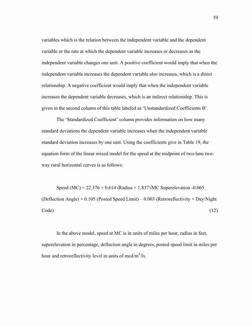
59

variables which is the relation between the independent variable and the dependent

variable or the rate at which the dependent variable increases or decreases as the

independent variable changes one unit. A positive coefficient would imply that when the

independent variable increases the dependent variable also increases, which is a direct

relationship. A negative coefficient would imply that when the independent variable

increases the dependent variable decreases, which is an indirect relationship. This is

given in the second column of this table labeled as ‘Unstandardized Coefficients B’.

The ‘Standardized Coefficient’ column provides information on how many

standard deviations the dependent variable increases when the independent variable

standard deviation increases by one unit. Using the coefficients give in Table 19, the

equation form of the linear mixed model for the speed at the midpoint of two-lane two-

way rural horizontal curves is as follows:

Speed (MC) = 22.376 + 0.614√Radius + 1.837√MC Superelevation -0.065

(Deflection Angle) + 0.105 (Posted Speed Limit) – 0.003 (Retroreflectivity × Day/Night

Code) (12)

In the above model, speed at MC is in units of miles per hour, radius in feet,

superelevation in percentage, deflection angle in degrees, posted speed limit in miles per

hour and retroreflectivity level in units of mcd/m2/lx.

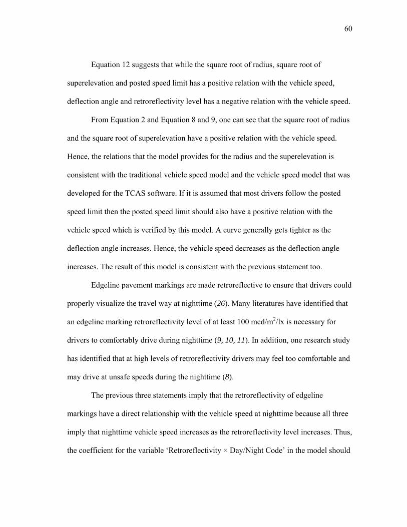
60

Equation 12 suggests that while the square root of radius, square root of

superelevation and posted speed limit has a positive relation with the vehicle speed,

deflection angle and retroreflectivity level has a negative relation with the vehicle speed.

From Equation 2 and Equation 8 and 9, one can see that the square root of radius

and the square root of superelevation have a positive relation with the vehicle speed.

Hence, the relations that the model provides for the radius and the superelevation is

consistent with the traditional vehicle speed model and the vehicle speed model that was

developed for the TCAS software. If it is assumed that most drivers follow the posted

speed limit then the posted speed limit should also have a positive relation with the

vehicle speed which is verified by this model. A curve generally gets tighter as the

deflection angle increases. Hence, the vehicle speed decreases as the deflection angle

increases. The result of this model is consistent with the previous statement too.

Edgeline pavement markings are made retroreflective to ensure that drivers could

properly visualize the travel way at nighttime (26). Many literatures have identified that

an edgeline marking retroreflectivity level of at least 100 mcd/m2/lx is necessary for

drivers to comfortably drive during nighttime (9, 10, 11). In addition, one research study

has identified that at high levels of retroreflectivity drivers may feel too comfortable and

may drive at unsafe speeds during the nighttime (8).

The previous three statements imply that the retroreflectivity of edgeline

markings have a direct relationship with the vehicle speed at nighttime because all three

imply that nighttime vehicle speed increases as the retroreflectivity level increases. Thus,

the coefficient for the variable ‘Retroreflectivity × Day/Night Code’ in the model should

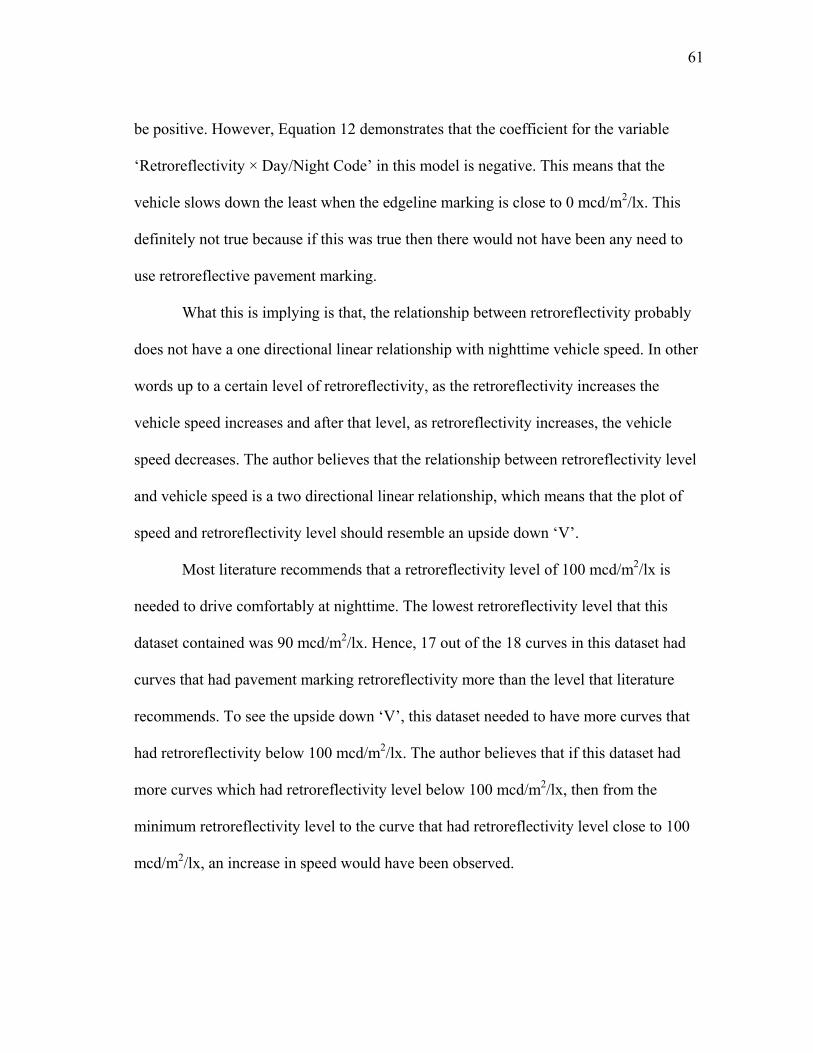
61

be positive. However, Equation 12 demonstrates that the coefficient for the variable

‘Retroreflectivity × Day/Night Code’ in this model is negative. This means that the

vehicle slows down the least when the edgeline marking is close to 0 mcd/m2/lx. This

definitely not true because if this was true then there would not have been any need to

use retroreflective pavement marking.

What this is implying is that, the relationship between retroreflectivity probably

does not have a one directional linear relationship with nighttime vehicle speed. In other

words up to a certain level of retroreflectivity, as the retroreflectivity increases the

vehicle speed increases and after that level, as retroreflectivity increases, the vehicle

speed decreases. The author believes that the relationship between retroreflectivity level

and vehicle speed is a two directional linear relationship, which means that the plot of

speed and retroreflectivity level should resemble an upside down ‘V’.

Most literature recommends that a retroreflectivity level of 100 mcd/m2/lx is

needed to drive comfortably at nighttime. The lowest retroreflectivity level that this

dataset contained was 90 mcd/m2/lx. Hence, 17 out of the 18 curves in this dataset had

curves that had pavement marking retroreflectivity more than the level that literature

recommends. To see the upside down ‘V’, this dataset needed to have more curves that

had retroreflectivity below 100 mcd/m2/lx. The author believes that if this dataset had

more curves which had retroreflectivity level below 100 mcd/m2/lx, then from the

minimum retroreflectivity level to the curve that had retroreflectivity level close to 100

mcd/m2/lx, an increase in speed would have been observed.

62

By observing the coefficients for the independent variables in the above

equation, one might think that the superelevation has greater impact on speed compared

to the other variables that has been used in the model because it has the largest

coefficient value among the five variables. However, that is not the case.

In the above equation, the radius of the curve actually has the biggest impact on

speed even though it has a smaller coefficient value than the superelevation. This is

because the numerical value of a radius is much larger than the numerical value of a

superelevation. For example, in this dataset the curve with the smallest radius had a

radius of 318 ft. Hence, according to this model, for this radius the vehicle speed would

increase by 17.8 mph (0.614√318). On the other hand, the curve with the largest

superelevation in the dataset had a superelevation of 13.2 percent. According to the

model created here, this superelevation would increase the vehicle speed by 6.5 mph

(1.837√13.2). Thus, even though superelevation has a higher coefficient than the radius,

the smallest radius in the dataset impacts the vehicle speed more than the largest

superelevation because of the magnitude of a radius is much larger than superelevation.

The curve with the highest posted speed limit in this dataset had a speed limit of

55 mph. This speed limit would increase the vehicle speed by 5.8 mph (0.105 × 55). The

highest deflection angle in this dataset was 92, which would decrease the speed by 6

mph (0.065 × 92). The largest retroreflectivity level was 479 which would decrease the

speed by only 1.4 mph (0.003 × 479). Hence, one can see that according to the model

that was developed in Equation 12, radius has the largest impact on vehicle speed. This

63

is definitely why all the vehicle speed models that were developed in the past had radius

as one of the independent variables.

Model 2 (Stepwise Regression Analysis)

Column 2 and column 3 of Table 20 located in Appendix B demonstrates which

variables were entered and which variables were excluded in each step to develop the

model. Model 1 suggested that all the variables were significant in predicting the vehicle

speed. As a result the stepwise regression did not remove any of the independent

variables. In each step, it just added another variable. The R-square column in Table 21

of Appendix B indicates that the R-square of the models in each step improved. This

means that the inclusion of each variable improved the R-square of the model and thus,

the final model should include all of these five variables which are radius,

superelevation, posted speed limit, deflection angle and retroreflectivity of pavement

edgeline marking with nighttime speed data. The author did not examine the residual

plot or the histogram plot for this model as this model as mentioned before was identical

to Model 1. The author is also not going to provide the equation for this model as it is

identical to Model 1 too.

COMPARISON OF DAYTIME AND NIGHTTIME SPEED USING SIDE

FRICTION DEMAND AND RETROREFLECTIVITY

The following paragraphs discussed the ANOVA test that compared the daytime

and nighttime speed at the midpoint of the curve for the six different methods. Prior to

64

that, the author provides the average daytime and nighttime speed for each curve in the

Table 5 below.

Table 5 Average Daytime and Nighttime Speed for Each Curve Curve

ID Average Daytime

Speed (mph) Average Nighttime

Speed (mph) 1 37.5 37.4 2 41.3 41.5 4 46.8 47 7 47.7 47.2 8 43.9 43.5 10 50.3 50.3 15 42.9 39.7 29 46.4 46.4 30 38.1 38.2 31 44.3 44.3 32 49.6 49.5 33 56.1 56.3 35 51.1 51.2 37 49.6 49.8 38 50.1 50.1 39 57.8 57.9 40 55.2 55.5 53 55.8 55.7

Method 1

Before comparing the daytime and nighttime speed, the first step consisted of

verifying whether each group met the minimum sample size requirement. Table 6 on the

next page provides some of the basic statistics for each group in this method obtained

from SPSS.

65

Table 6 Method 1 Descriptive Statistics Group N Mean Std. Deviation Std. Error A_D 6108 52.71 6.81 .08 A_N 615 51.64 6.82 .27 B_D 4897 45.74 6.58 .09 B_N 351 46.35 7.32 .39 C_D 7526 42.93 6.33 .07 C_N 639 42.46 6.89 .27

In the group column, the first letter corresponds to the group and the second letter

denotes the light condition (D for day and N for night). In the Data Analysis section, it

was mentioned that a minimum of 100 vehicles was to be used for each group. From the

above table it can be observed that all of the groups for both daytime and nighttime had

more than 100 vehicles. Thus, each group met the minimum sample size requirement

that was set for this analysis.

The first null hypothesis (H0) stated that within a group there was statistical


curve while the first alternative hypothesis (HA) stated that within a group there was no

statistical significant speed difference between the daytime and nighttime speed at the

midpoint of the curve.

As Group C had curves with higher side friction demand value compared to the

other two groups, it was assumed that for this group, the daytime and nighttime speed

difference would be significant and this difference would be higher than the daytime and

nighttime speed difference of Group A and B. As Group A contained flatter curves or

curves with a side friction demand value of 0; the daytime and nighttime speed may not

66

be significantly different for Group A. Since Group B contained curves that had a side

friction demand value more than 0 but not as high as curves in Group C, it was hard to

make any assumption about the speed difference.

As mentioned in the Data Analysis section, Tukey test was conducted for each

method which is part of the One-way ANOVA test. Only the result of the Tukey test was

discussed because it is easier to compare the speeds for each group in the Tukey test

result. The Tukey test results table labeled as ‘Multiple Comparisons’, for this method is

given in Table 22 of Appendix C. In this table, column 3 provides the mean speed

difference between two groups and column 5 labeled as ‘Sig.’ contains the p-values,

which indicates whether the difference in column 3 is statistically significant or not. A p-

value of 0.05 or less corresponds to the two groups being statistically significantly

different at a 95 percent confidence level. To make the p-values easier to visualize when

it is 0.05 or less, SPSS puts an asterisk beside the mean difference value in column 3. A

positive value in column 3 suggests that the mean speed decreased from column 1 to

column 2.

The results of Table 22 suggest that for Group A the daytime and nighttime

speeds were significantly different statistically while for Group B and Group C the

daytime and nighttime speeds were not significantly different statistically. Thus, while

the null hypothesis was true for Group A, for Group B and C the alternative hypothesis

was true.

Unfortunately, the results of the analysis contradict the assumptions made by the

author. However, there is a reason for that. The assumptions that were made by the

67

author may have been correct if side friction demand was the only dependent variable

and other variables such as retroreflectivity were kept constant. However, that was not

the case for this method. For example, even though Group A had flatter curves, it

contained curves with pavement markings with a wide range of retroreflectivity value.

Thus, at curves with low retroreflectivity levels, vehicles may have been slowing down

significantly at night compared to daytime. In addition to that the overall speed data in

Group A may have been dominated by curves with lower retroreflectivity levels rather

than curves with higher retroreflectivity levels. As a result, the daytime speed was

significantly higher than the nighttime speed.

After observing the daytime and nighttime speed differences of Group B and C,

the author concluded that the daytime and nighttime speed for these groups are the same

because the difference between the speed for the two light conditions for these two

groups are less than 1 mph, which the author considers to be negligible.

The second null hypothesis (H0) stated that, for the same light condition, there

was a statistical significant speed difference between two consecutive groups. The

alternate hypothesis (HA) stated that for the same light condition, there was no statistical

significant speed difference between two consecutive groups.

In the Data Analysis section it was mentioned that in this method side friction

demand value increases from Group A to Group C or curves become sharper from

Group A to Group C. Hence, the vehicle mean speed should decrease from Group A to

Group C. The average speed values in ‘Mean’ column of Table 6 are consistent with this

68

assumption. Group A has the highest mean speed while Group C has the lowest mean

speed.

The null hypothesis which stated that there was a statistical significant speed

difference between two groups of the same light condition was true for all the three

groups. For the daytime groups, Group A_D had significantly higher speed than Group

B_D and Group B_D had significantly higher speeds than Group C_D. For the nighttime

groups, Group A_N had significantly higher speed than Group B_N and Group B_N had

significantly higher speeds than Group C_N. This verified that vehicle speed does

decrease as the side friction of the curve increases. In addition, it proved that the

categorizing of the curves in terms of side friction demand had been done properly. If

the curves were not categorized properly then this significant difference in speed would

not have been observed.

The author could not conclude anything from the difference between the daytime

and nighttime speeds for the three groups that were analyzed but this method verified

that as the side friction demand increases, the vehicle speed decreases at the midpoint of

the curve on two-lane two-way rural horizontal curves.

Method 2

The Data Analysis section stated that this method was exactly the same as the

previous method except that Curve 30, which was in Group C in Method 1, was removed

from the analysis here. Thus, the results for Group A and Group B of this method and

Method 1 are identical as they have been kept unchanged. Table 7 below which provides

69

the descriptive statistics for this method demonstrates that all of the groups met the

minimum sample size requirement.


Only the results of Group C were analyzed here. To avoid redundancy the results

of Group A and Group B were not analyzed since Group A and Group B of this method

are the same Group A and Group B of Method 1.

The first hypothesis focused on the daytime and nighttime speed difference. In

the previous method, it was assumed that for Group C, the speed difference between the

daytime and nighttime vehicles would be significant because it contained curves with

higher side friction demand compared to the other two groups. Group C of this method

was exactly the same as Group C of method 1 except that curve 30 which had the highest

side friction demand (0.12) among all the curves being analyzed was excluded from the

analysis. Since even after having the curve with the highest side friction demand value

the daytime and nighttime speed difference of Group C in the previous method was not

statistically significant, the author predicted that, in this group too the difference would

not be significant.

70

Tukey test result in Table 23 of Appendix C is consistent with this assumption

that the speed differences between the daytime and nighttime vehicles were not

significant in Group C. This meant that the alternative hypothesis was true that there was

no significant difference in daytime and nighttime speed. Infact, since the difference was

less than one mile per hour, the author believes that the daytime and nighttime speeds

were the same.

The second hypothesis focused on the speed difference between two consecutive

groups. As Group C has sharper curves than Group B, it was assumed that the vehicle

speed in Group C was significantly lower than the vehicle speed in Group B for both

daytime and nighttime vehicles. The Tukey test results of this method given in Table 23

Appendix C demonstrate that Group B_D had significantly higher speed than Group

C_D and Group B_N has significantly higher speed than Group C_N. Hence, this proved

the null hypothesis that there was a significant speed difference between the vehicle

speeds of two groups with the same light condition.

Similar to Method 1, the results of this method suggested that as the side friction

demand increases, vehicle speed decreases at the midpoint of the curve on two-lane two-

way rural horizontal curves.

Method 3

In the previous two methods, side friction was divided into three groups. In this

method, side friction was categorized in to two groups. Here, Group A was the

combination of Group and Group B of Method 2 and Group B was the Group C of

Method 2. To avoid repetition, Group C was not discussed here anymore. Data from

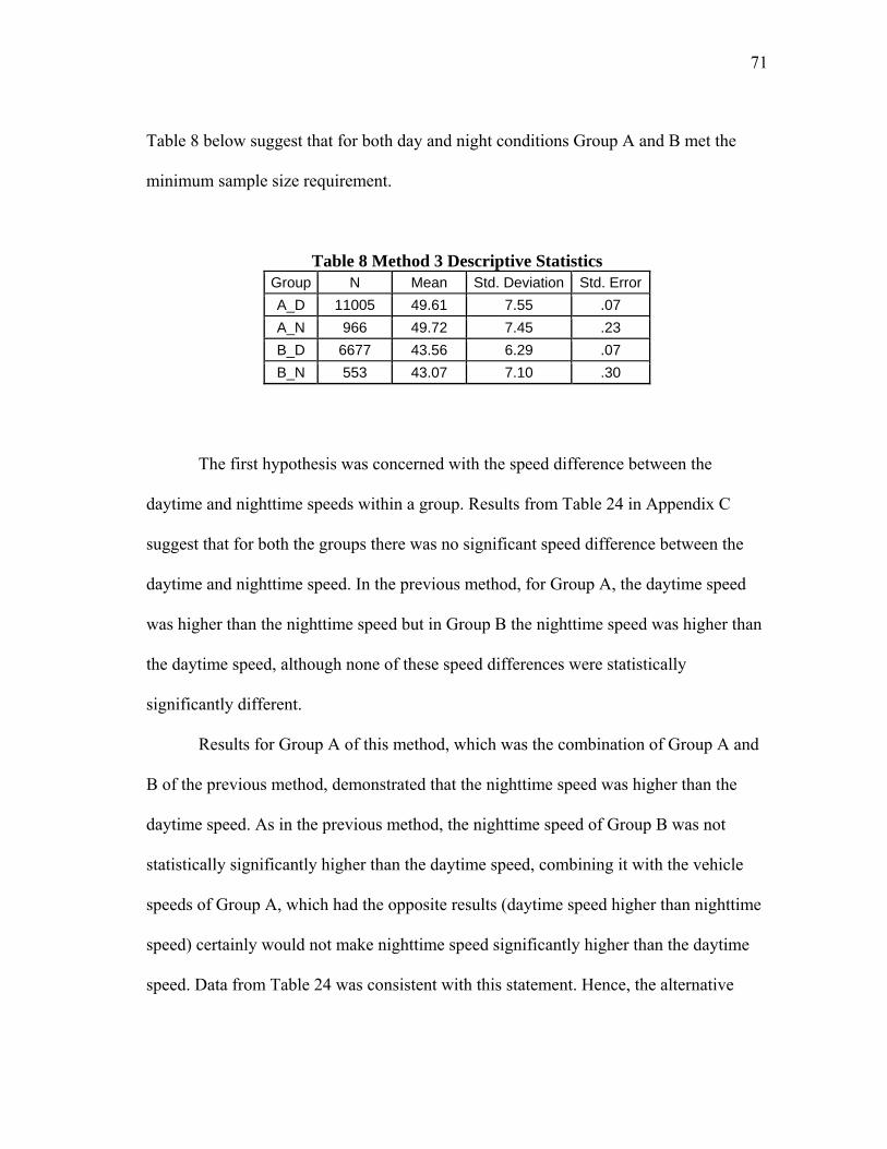
71

Table 8 below suggest that for both day and night conditions Group A and B met the

minimum sample size requirement.

Table 8 Method 3 Descriptive Statistics Group N Mean Std. Deviation Std. Error A_D 11005 49.61 7.55 .07 A_N 966 49.72 7.45 .23 B_D 6677 43.56 6.29 .07 B_N 553 43.07 7.10 .30

The first hypothesis was concerned with the speed difference between the

daytime and nighttime speeds within a group. Results from Table 24 in Appendix C

suggest that for both the groups there was no significant speed difference between the

daytime and nighttime speed. In the previous method, for Group A, the daytime speed

was higher than the nighttime speed but in Group B the nighttime speed was higher than

the daytime speed, although none of these speed differences were statistically

significantly different.

Results for Group A of this method, which was the combination of Group A and

B of the previous method, demonstrated that the nighttime speed was higher than the

daytime speed. As in the previous method, the nighttime speed of Group B was not

statistically significantly higher than the daytime speed, combining it with the vehicle

speeds of Group A, which had the opposite results (daytime speed higher than nighttime

speed) certainly would not make nighttime speed significantly higher than the daytime

speed. Data from Table 24 was consistent with this statement. Hence, the alternative

72

hypothesis, which stated that there was no significant speed difference between the

daytime and nighttime vehicles, was true for both of these groups. The author concluded

that the daytime and nighttime speeds for these two groups were actually the same as the

speed difference was within 1 mph.

The second hypothesis was concerned with the speed difference between two

consecutive groups. From Table 24 it can be observed for the daytime groups, Group

A_D has a significantly higher speed than Group B_D and for the nighttime groups,

Group A_N has a significantly higher speed than Group B_N. This proved the null

hypothesis which stated that there was a significant difference in speed between

consecutive two groups with the same light condition. Once again, this proves that

vehicle speed decreases as the side friction of the curve increases and that the

categorizing of the curves in terms of side friction demand had been done properly. This

is why the significant difference in speed was observed. It was very important to

categorize the curves properly in this method because the technique used in this method

to categorize the curves in terms of side friction was used in the following three methods

too.

Similar to the previous two methods, from this method too the author was not

able to conclude anything from the difference between the daytime and nighttime speed

but was able to verify that vehicle speed decreases at the midpoint of the curve on two-

lane two-way rural horizontal curves.

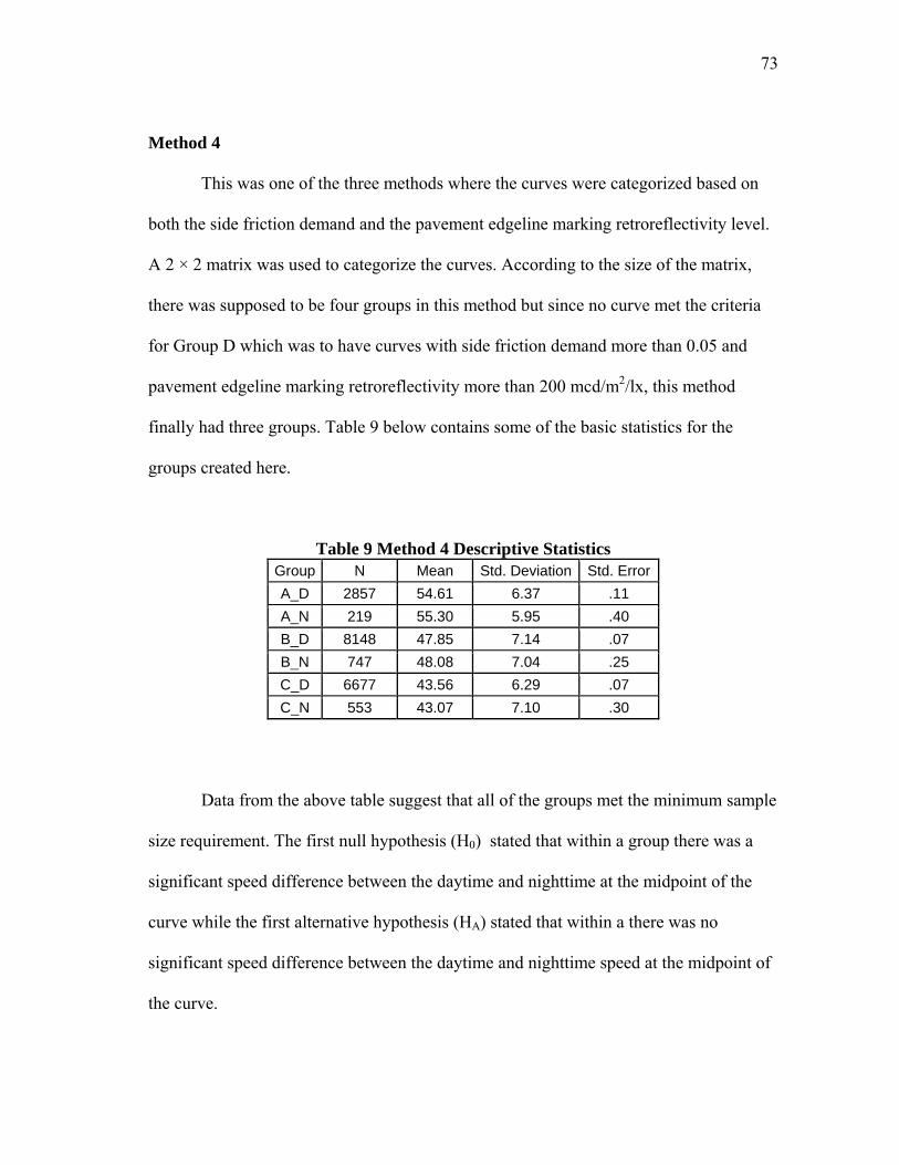
73

Method 4

This was one of the three methods where the curves were categorized based on

both the side friction demand and the pavement edgeline marking retroreflectivity level.

A 2 × 2 matrix was used to categorize the curves. According to the size of the matrix,

there was supposed to be four groups in this method but since no curve met the criteria

for Group D which was to have curves with side friction demand more than 0.05 and

pavement edgeline marking retroreflectivity more than 200 mcd/m2/lx, this method

finally had three groups. Table 9 below contains some of the basic statistics for the

groups created here.


Data from the above table suggest that all of the groups met the minimum sample

size requirement. The first null hypothesis (H0) stated that within a group there was a


curve while the first alternative hypothesis (HA) stated that within a there was no

significant speed difference between the daytime and nighttime speed at the midpoint of

the curve.

74

From Table 2, located in the Data Analysis section it can be assumed that Group

B would have the least difference between the daytime and nighttime speed as this group

had curves with lower side friction demand and higher retroreflectivity level and the

nighttime speed maybe higher than the daytime speed since it had curves with higher

range of retroreflectivity levels. In addition, Group C would have the largest difference

between the daytime and nighttime speed among the three groups because curves in this

group high side friction demand value and low retroreflectivity level which are assumed

to effect vehicle speed negatively.

To test the above hypotheses, Table 25 of Appendix C, which contains the speed

comparisons of these groups, was observed. The speed comparisons suggest that the

largest difference between daytime and nighttime speed occurred in Group A followed

by Group C and B respectively. Not only for Group B but also for Group A the

nighttime speed was higher than the daytime speed. Group B_N had curves with

retroreflectivity more than 200 mcd/m2/lx. Thus, from the results of Group B_D and

Group B_N the author could conclude that at curves with edgeline markings having

retroreflectivity level of 200 mcd/m2/lx or more, vehicle speed during the nighttime is

higher than the vehicle speed during the daytime.

However, as the difference in the daytime and nighttime speed was only 0.2 mph

which was neither a statistically significant difference nor a practically significant

difference, the author would not conclude this. A statistical significant difference would

occur when the p-value 0.05 or less but a practical significant difference would occur

when the speed difference is more than 1 mph. As the speed difference is neither

75

statistically significantly different nor practically different, the author states that the

daytime and nighttime speed for Group B was the same.

The author assumed that Group A had curve or curves that had retroreflectivity

level close to 200 mcd/m2/lx (i.e. 190 mcd/m2/lx) and at these curve or curves the

nighttime speed was higher than the daytime speed. In addition, these curves had more

data, which was why results of these curves were dominating the overall result. From

Table 2 the author determined that no curves in Group A had retroreflectivity close to

200 mcd/m2/lx. The curve with the highest retroreflectivity level in this group had a

retroreflectivity level of 150 mcd/m2/lx. Hence, the author believes there was something

else other than the retroreflectivity level which was made the nighttime speed higher

than the daytime speed in Group A.

One explanation of this is that since these curves were located in rural areas, the

percentage of drivers who were familiar with these curves was more at nighttime than

daytime. As they were used to driving on these curves, the low retroreflectivity level did

not impact their speed. This was why the nighttime speed was higher than the daytime

speed. The author also considered that the speed for the daytime and nighttime was the

same as the difference in speed between the two light conditions was within 1 mph.

For Group C, the nighttime speed was lower than the daytime speed but not

significantly. Furthermore, Group B had a lower difference between the vehicle speeds

for the two light conditions than Group C which was assumed by the author. All three

groups prove the alternative hypothesis that there was no significant difference in speed

between the daytime and nighttime vehicles within a group and since these differences in

76

speed for the two light conditions for all three groups are within 1 mph, the author

believes that each of the three groups had the same day and night speed.

ANOVA test results from Table 25 suggest that the results for the second

hypothesis test were consistent with the results of the second hypothesis test for the

previous methods. Hence, the null hypothesis that there was a significant difference in

speed in two consecutive groups for the same light condition was true for all three

groups. For the daytime groups, Group A_D had statistically significantly higher speed

than Group B_D and Group B_D had a statistically significantly higher speed than

Group C_D. For the nighttime groups, Group A_N had statistically significantly higher

speed than Group B_N and Group B_N had statistically significantly higher speed than

Group C_N.

During daytime, it was assumed that vehicle speed is impacted by side friction

demand only and not the retroreflectivity level. This was why in the mixed linear model

for the daytime vehicles; only side friction demand was used as the independent

variable. According to this assumption, there should not be any significant difference in

speed between Group A_D and Group B_D because curves in this group had the same

range of side friction demand (<0.05). This meant that besides side friction demand

something else might have impacted the vehicle speed. The author predicted that the

posted speed limit impacted the vehicle speed.

Even though the posted speed limit was one of the variables used in the

calculation of side friction demand by the TCAS software, the author believed that there

was a need to analyze the effect of posted speed limit separately because in the

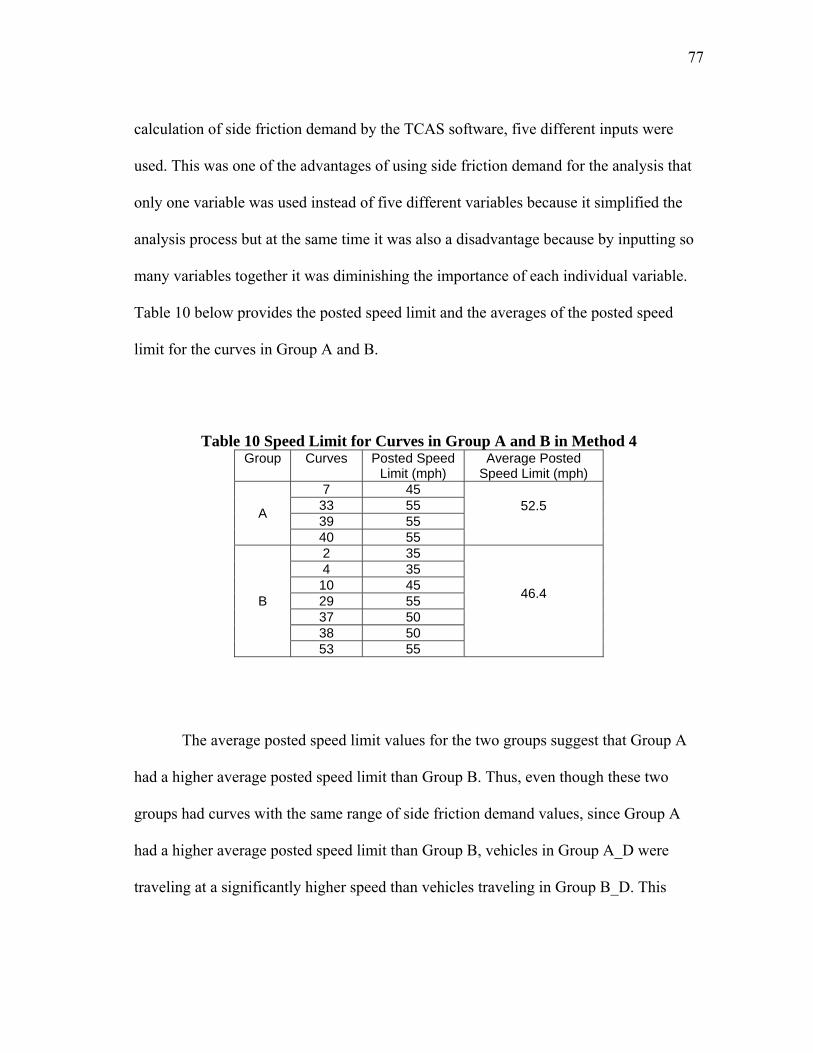
77

calculation of side friction demand by the TCAS software, five different inputs were

used. This was one of the advantages of using side friction demand for the analysis that

only one variable was used instead of five different variables because it simplified the

analysis process but at the same time it was also a disadvantage because by inputting so

many variables together it was diminishing the importance of each individual variable.

Table 10 below provides the posted speed limit and the averages of the posted speed

limit for the curves in Group A and B.

Table 10 Speed Limit for Curves in Group A and B in Method 4 Group Curves Posted Speed

Limit (mph) Average Posted

Speed Limit (mph)

A

7 45 52.5

33 55 39 55 40 55

B

2 35

46.4

4 35 10 45 29 55 37 50 38 50 53 55

The average posted speed limit values for the two groups suggest that Group A

had a higher average posted speed limit than Group B. Thus, even though these two

groups had curves with the same range of side friction demand values, since Group A

had a higher average posted speed limit than Group B, vehicles in Group A_D were

traveling at a significantly higher speed than vehicles traveling in Group B_D. This

78

suggested that it was important to analyze the impact of the posted speed limit separately

even though it has been used to calculate side friction demand.

For the nighttime groups, Group A_N had a significantly higher speed than

Group B_N even though the latter group had curves with higher retroreflectivity level.

This meant that for these groups the posted speed limit impacted the vehicle speed more

than the retroreflectivity level.

The reasoning for Group C having significantly lower vehicle speed than Group

B for both light conditions was that Group C had higher side friction demand than Group

B. In addition, Group C_N had curves with lower retroreflectivity level than Group B_N

and it was assumed that lower retroreflectivity level impacted speed negatively during

nighttime. The impact of retroreflectivity level on nighttime vehicles would have been

understood better if Group D_N could be compared to Group C_N because in that case

only retroreflectivity level would have been the variable. Unfortunately due to a lack of

curves in Group D_N the author could not conduct that comparison.

From this method, the author determined that at curves with edgeline markings

having retroreflectivity levels of 200 mcd/m2/lx or more, vehicles at nighttime may

travel at a higher speed than vehicles traveling during the day. In addition, it may be

necessary to analyze the impact of the posted speed limit separately on vehicle speed

even though it has already been incorporated into the calculation of side friction demand

Method 5

In this method the curves were grouped in terms of side friction demand, using

the same technique used in Method 3 and 4. In the previous method, the author

79

arbitrarily chose 200 mcd/m2/lx as the threshold to create the two retroreflectivity

groups. The author believes that the actual threshold point maybe different than that.

Thus, there maybe curves in the two groups that need to switch groups if the actual

threshold point was used. Since the actual threshold point is unknown, the author as

mentioned in the Data Analysis section, excluded curves having retroreflectivity

between 150 mcd/m2/lx and 250 mcd/m2/lx to better extinguish the difference between

the two retroreflectivity groups. After that the existing curves were grouped in two

groups, one containing curves less than 150 mcd/m2/lx and the other group containing

curves more than 250 mcd/m2/lx. Similar to Method 3, this created a 2 × 2 matrix, which

was supposed to yield four groups, but once again no curves met the criteria for Group D

(side friction demand >0.05 and retroreflectivity level >250 mcd/m2/lx), which is why at

the end there were three groups.


Values from Table 11 above imply that all the three groups had more than 100

vehicles for both types of light conditions. The first hypothesis focused on the

comparison of the daytime and nighttime vehicle speed within a group. To analyze the

80

results of this daytime and nighttime speed comparison, values in Table 26 of Appendix

C was observed.

The results of Method 4, determined that Group A and Group B had a higher

vehicle speed at nighttime compared to daytime but for Group C the daytime speed was

higher than the nighttime speed. The average retroreflectivity level of curves in Group B

of this method was higher than the average retroreflectivity level of curves in Group B of

the previous method. Since in Group B of the previous method, the nighttime speed was

found to be higher than the daytime speed, the same result is expected in Group B of this

method too. In addition, the author assumes that here the vehicle speed in Group B_N

might be actually significantly higher than the vehicle speed in Group B_D.

For Group A and C the author predicted the daytime speed to be higher than the

nighttime speed. Group B would have the least difference between the daytime and

nighttime speed as this group had curves with lower side friction demand and higher

retroreflectivity level. Furthermore, Group C would have the largest difference between

the daytime and nighttime speed among the three groups because curves in this group

had characteristics that are assumed to affect speed negatively which are high side

friction demand value and low retroreflectivity level.

The results of the Tukey test which compared the daytime and nighttime vehicle

speed for this method is given in Table 26 of Appendix C. The nighttime speeds for all

three groups were higher than the daytime speed but none of these differences were

statistically significant. For Group B, the author predicted that the nighttime speed may

be significantly greater than the daytime speed but in reality the nighttime was only 0.2

81

miles higher than the daytime speed. Thus, the author could not conclude with certainty

that at curves with edgeline markings having retroreflectivity level of 250 mcd/m2/lx or

more, vehicle speed during nighttime is higher than the daytime vehicle speed.

Group A of the previous method had Curves 7, 33, 39 and 40 while Group A of

this method had Curves 7, 39 and 40. Group A of this method, excluded Curve 33 from

the analysis to ensure sure that there was no curve with retroreflectivity level close to

200 mcd/m2/lx, which was assumed to be the retroreflectivity level above which drivers

at nighttime driver faster than the daytime. Thus, having curves with retroreflectivity

level close to 200 mcd/m2/lx was not the reason why Group A_N had a higher speed

than Group A_D because curves within 50 mcd/m2/lx of 200 mcd/m2/lx were excluded

in this method. The author believes that the reason why Group A in this method had a

higher nighttime speed than daytime speed was because of the same reason why Group

A had a higher nighttime speed than daytime speed in the previous method. Since the

difference in daytime and nighttime speed for Group A was more than 1 mph, the author

would not consider the daytime and nighttime speed to be the same though.

Group C of this method should not have the issue that was pointed out in Group

A of the previous method, which was having curves with retroreflectivity close to 200

mcd/m2/lx. This was because as mentioned in the previous paragraph, this method

excluded curves within 50 mcd/m2/lx of 200 mcd/m2/lx. The author believes the reason

why Group C_N had higher speed than Group C_D was because of the same reason why

Group A_N of this method and the previous method had a higher speed than Group A_D

of this method and the previous method. Due to a nonzero difference in speed between

82

daytime and nighttime, the author gave the explanation as to why it might have

happened but as this difference was less than 1 mph, the author considers the daytime

and nighttime speed to be the same.

For Group C, the nighttime speed was lower than the daytime speed. In addition,

Group B had a lower difference between the vehicle speeds for the two light conditions

than Group C which was assumed by the author. All three groups prove the alternative

hypothesis that there was no significant difference in speed between the daytime and

nighttime vehicles within a group.

To determine whether the null hypothesis or the alternative hypothesis was true

for the second hypothesis, the author observed the Tukey test results in Table 26 again.

As found in the previous methods, in this method too for both daytime and nighttime

each group had significantly higher speeds than the next group.

Similar to Method 4, in this method too both Group A and Group B had curves

with the same range of side friction demand value. The author believed that Group A_D

had a higher average posted speed limit than Group B_D, which is why vehicles in

Group A_D were traveling at a significantly higher speed than Group B_D. Table 12

provides the posted speed limit of the curves in this two groups and the average speed

limit for the two groups.

83

Table 12 Speed Limit for Curves in Group A and B in Method 5 Group Curves Posted Speed


Speed Limit (mph)

A 7 45

51.7 39 55 40 55

B

2 35

44 4 35 10 45 38 50 53 55

The above table demonstrates that group A had a significantly higher average

posted speed limit than Group B. The author believes that this is the reason why Group

A_D had a significantly higher speed than Group B_D.

Like in Method 4 in this method, even though, Group B_N had curves with

higher retroreflectivity than Group A_N, the vehicle speed of Group A_N was

significantly higher than Group B_N. The higher average posted speed limit of Group A

than Group B was the reason for this. Hence, for these groups the posted speed limit

impacted the vehicle speed more than the retroreflectivity level.

Having curves with higher side friction demand than Group B was the reason

why the daytime vehicles in Group C had significantly lower speed than the daytime

vehicles in Group B. Group C_N had significantly lower vehicle speed than Group B_N

because Group C had curves with higher side friction demand and lower pavement

edgeline marking retroreflectivity level compared to Group B. Once again, the effect of

retroreflectivity on vehicle speed would have been understood better if Group D existed.

This is because then Group D_N could have been compared to Group C_N where

84

retroreflectivity would have been the only variable. Unfortunately, due to a lack curves

in Group D, the author could not conduct the comparison.

The results of this method were identical to the results of the previous method.

The author determined that at curves with edgeline markings having retroreflectivity

level of 250 mcd/m2/lx or more, vehicle at nighttime may travel at a higher speed than

vehicles traveling at daytime. In addition, it might be necessary to analyze the impact of

the posted speed limit separately even though it has already been used to calculate side

friction demand.

Method 6

In this method both side friction demand and retroreflectivity were also used to

categorize the data. This method was identical to the previous method, except that in this

method, the curves that were excluded from the analysis in the previous method (curves

with retroreflectivity between 150 mcd/m2/lx and 250 mcd/m2/lx) were included in the

analysis by forming a different group for those curves. Hence, in this method there were

two groups for side friction demand and three groups for retroreflectivity level that

created a 2 × 3 matrix. Although, due to the size of the matrix there should have been six

groups, this method had five groups as there were no curves that met the criteria for one

of the groups. The purpose of including the curves that were excluded in Method 5 by

forming a different group was to identify whether drivers traveling in these curves at

nighttime travel at a speed similar to drivers traveling at nighttime at curves with

retroreflectivity less than 150 mcd/m2/lx or if they travel at a speed similar to drivers

traveling at nighttime at curves with retroreflectivity more than 250 mcd/m2/lx or

85

whether their speed is significantly different from drivers traveling at curves with

edgeline markings less than 150 mcd/m2/lx and more than 250 mcd/m2/lx . Table 13

below contains some of the basic statistics for the groups created here.

Table 13 Method 6 Descriptive Statistics Group N Mean Std. Deviation Std. Error A_D 2449 54.33 6.40 .12 A_N 176 55.54 5.82 .43 B_D 2600 49.56 6.72 .13 B_N 242 49.66 7.31 .47 C_D 5956 47.69 7.48 .09 C_N 548 47.87 7.01 .29 D_D 2523 45.08 5.59 .11 D_N 216 45.71 6.06 .41 E_D 4154 42.64 6.50 .10 E_N 337 41.37 7.21 .39

The above table demonstrates that each group met the minimum sample size

requirement of 100 vehicles. The Tukey test results for this method are located in Table

27 of Appendix C. First the author focused on the results of the first hypothesis which

was to examine the difference between the daytime and nighttime speed for each group.

Results of Group A, C and D were not discussed as they are the same as Group

A, B and C of the previous method. In Group B, the nighttime speed was greater than the

daytime speed but since the speed difference was not significant and was within 1 mph

the author considers the daytime and nighttime speed of Group B to be the same.

For Group E the daytime speed was significantly greater than the nighttime

speed. This result was contradictory to the results found in literature. Literature stated

86

that at higher retroreflectivity levels, vehicle drive at unsafe speeds during nighttime (8).

If retroreflectivity level between 150 mcd/m2/lx and 250 mcd/m2/lx is considered high

retroreflectivity level then the result of Group E contradicts the previous statement. In

that case the nighttime speed for Group E should have been higher than the daytime

speed or should have been at least the same as the daytime speed. However, the opposite

had happened.

From the result of this group, the author could conclude that despite the

retroreflectivity level, at curves with side friction level more than 0.05, drivers drive

significantly slower at night time compared to the daytime. The issue is that if this was

true then, in Group D too, the nighttime speed would have been significantly slower than

the daytime speed but that did not happen. The author finally concluded that, at curves

with side friction demand more than 0.05 and with pavement edgeline marking

retroreflectivity level between 150 mcd/m2/lx and 250 mcd/m2/lx, drivers drive

significantly slower at nighttime than during the daytime. This was because, due to the

high retroreflectivity level, drivers are better aware of the sharpness of the curve then

they would have at lower levels of retroreflectivity level. This led them to slow down. At

curves with side friction demand more than 0.05 and edgeline marking retroreflectivity

level less than 150 mcd/m2/lx drivers do not slow down because the author believes that

they are not able to judge the sharpness of the curve and may even underestimate the

sharpness of the curve.

In the Linear Mixed Model section, the author planned to determine the

retroreflectivity level where the relationship between retroreflectivity and vehicle speed

87

changes. From the result of this group, the author determines that for curves with side

friction demand more than 0.05, retroreflectivity level of 150 mcd/m2/lx is where the

relationship between retroreflectivity level and vehicle speed at night changes.

However, to determine whether this relationship between retroreflectivity and

nighttime vehicle speed stays the same (as retroreflectivity level is more than 250

mcd/m2/lx, nighttime vehicle speed decreases), the author need to examine Group F,

which was supposed to have curves with side friction demand greater than 0.05 and

edgeline marking retroreflectivity more than 250 mcd/m2/lx. Due to a lack of curves in

Group F, the author could not be certain whether for curves with side friction demand

greater than 0.05 and edgeline marking retroreflectivity level greater than 250

mcd/m2/lx, daytime vehicle speed is significantly greater than the nighttime vehicle

speed or whether for retroreflectivity level greater than 250 mcd/m2/lx, the relationship

switches again and the nighttime speed becomes greater than the daytime speed.

From the first hypothesis, the author determines that regardless of the

retroreflectivity level, for curves with side friction demand less than 0.05, the daytime

and nighttime speeds are similar. For curves with side friction demand greater than 0.05

and pavement edgeline marking retroreflectivity level between 150 mcd/m2/lx and 250

mcd/m2/lx, the daytime speed was significantly higher than the nighttime speed.

The purpose of the second hypothesis was to compare the speed differences

between consecutive groups for the same light condition. One-way ANOVA test results

provided for this method in Table 27 suggested that each group had a significantly

88

higher speed for both daytime and nighttime than the next group’s daytime and

nighttime speed, proving the null hypothesis.

For the daytime groups the only statistical significant difference in speed should

have been between Group C_D and Group D_D because these two consecutive groups

had curves with different ranges of side friction demand. Groups A_D, B_D and C_D

should have the same or similar speeds because these groups had curves with the same

range of side friction demand while Group D_D and Group E_D should have the same

or similar speeds because these two groups contained curves with the same range of side

friction demand. The author predicted that the difference in the average posted speed

limit between each consecutive group caused the significant difference in speed. The

average posted limit for each group is presented below in Table 14.

Table 14 Speed Limit for Curves in Method 6 Group Curves Posted Speed


Speed Limit (mph)

A 7 45

51.7 39 55 40 55

B 29 55

53.3 33 55 37 50

C

2 35

44.0 4 35 10 45 38 50 53 55

D 8 45

51.7 31 55 35 55

E 1 35

48.3 15 55 32 55

89

Tukey test results demonstrated that Group A had significantly higher daytime

speed than Group B. However, from the above table it can be observed that Group B had

a higher average posted speed limit than Group A. This led the author to observe the

average speeds of the curves in Group A and B given in Table 5. From Table 5 the

author determined that even though Curve 29 which was in Group B, had a posted speed

limit of 55 mph, the average daytime vehicle speed was only 46.4 mph. The author

determined that the presence of a t-leg intersection upstream of the midpoint of the curve

caused the average vehicle speed to be considerably lower than the posted speed limit at

Curve 29. For this reason, Group A had a higher average daytime speed than Group B

despite having a lower average posted speed limit than Group B.

For having a higher posted average posted speed limit, Group B had a higher

average daytime speed than Group C and Group D had a higher average daytime speed

than Group E. As mentioned previously, Group C_D had a higher daytime speed than

Group D_D because vehicles in Group D_D were traveling on sharper curves compared

to Group C_D.

For the nighttime groups too, the author believes that the speed difference

between the consecutive groups had been caused mainly due to the posted speed limit

and the side friction demand. The effect of retroreflectivity is very hard to determine.

Among groups A, B and C and groups D and E, the effect of retroreflectivity could have

been determined only if both the side friction demand and the posted speed limit were

kept constant.

90

Out of the six methods, the author believes that the finding from this method

was the most important. From the results of this method the author determined that at

curves with side friction demand more than 0.05 and with pavement edgeline marking

retroreflectivity between 150 mcd/m2/lx and 250 mcd/m2/lx drivers drive slower at

nighttime than during the daytime because the enhanced retroreflectivity actually helps

driver become more aware of the curvature of the road, which leads them to slow down.

At curves with side friction demand greater than 0.05 and with pavement edgeline

marking retroreflectivity up to 150 mcd/m2/lx drivers underestimate the curvature and

the road conditions and hence do not feel the need to slow down. Finally, the author

believes that for curves with side friction demand greater than 0.05, a pavement edgeline

marking retroreflectivity level of 150 mcd/m2/lx is where the relationship between

retroreflectivity and vehicle speed changes direction.

COMPARISON OF DAYTIME AND NIGHTTIME SPEED USING RADIUS

AND RETROREFLECTIVITY

The following paragraphs discussed the ANOVA test that compared the daytime

and nighttime speed at the midpoint of the curve for the two methods.

Method 7

The basic statistics for this method are provided in the table below and the

ANOVA test results for this method is provided in Table 28 of Appendix C.

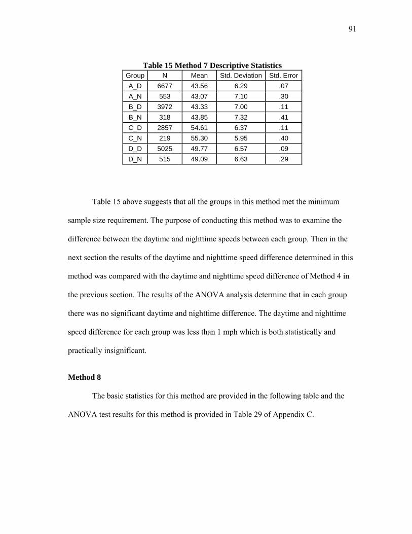
91

Table 15 Method 7 Descriptive Statistics Group N Mean Std. Deviation Std. Error A_D 6677 43.56 6.29 .07 A_N 553 43.07 7.10 .30 B_D 3972 43.33 7.00 .11 B_N 318 43.85 7.32 .41 C_D 2857 54.61 6.37 .11 C_N 219 55.30 5.95 .40 D_D 5025 49.77 6.57 .09 D_N 515 49.09 6.63 .29

Table 15 above suggests that all the groups in this method met the minimum

sample size requirement. The purpose of conducting this method was to examine the

difference between the daytime and nighttime speeds between each group. Then in the

next section the results of the daytime and nighttime speed difference determined in this

method was compared with the daytime and nighttime speed difference of Method 4 in

the previous section. The results of the ANOVA analysis determine that in each group

there was no significant daytime and nighttime difference. The daytime and nighttime

speed difference for each group was less than 1 mph which is both statistically and

practically insignificant.

Method 8

The basic statistics for this method are provided in the following table and the

ANOVA test results for this method is provided in Table 29 of Appendix C.

92

Table 16 Method 8 Descriptive Statistics Group N Mean Std. Deviation Std. Error A_D 2523 45.08 5.59 .11 A_N 216 45.71 6.06 .41 B_D 1802 41.24 5.18 .12 B_N 116 41.57 5.27 .48 C_D 2449 54.33 6.40 .12 C_N 176 55.54 5.82 .43 D_D 4154 50.48 6.54 .10 D_N 432 49.56 6.44 .31

Table 16 above indicates that all groups met the minimum sample size

requirement. Once again, the purpose of conducting this method was to compare the

daytime and nighttime speed difference determined in this section to the daytime and

nighttime speed difference of Method 5 of in the previous section. The ANOVA test

results for this method suggests that for each group there was no significant speed

difference between the daytime and nighttime speed. The maximum daytime and

nighttime speed difference occurred in group C which was only 1.2 mph. For the other

groups it was less than 1 mph. Hence, for each group the author states that the daytime

and nighttime speeds are the same as the difference is both statistically and practically

insignificant.

93

RESULTS OF COMPARISONS OF DAYTIME AND NIGHTTIME SPEED

USING SIDE FRICTION DEMAND AND RETROREFLECTIVITY AND

RADIUS AND RETROREFLECTIVITY

Method 4 and Method 5 of Comparison of Daytime and Nighttime Speed Using

Side Friction Demand and Retroreflectivity section were very similar to Method 7 and

Method 8 of Comparison of Daytime and Nighttime Speed Using Radius and

Retroreflectivity section. The only difference is that the first two methods used side

friction demand and retroreflectivity level to categorize the curves and the latter two

methods used radius and retroreflectivity to categorize the curves. Method 4 used the

same retroreflectivity threshold value as Method 7 while Method 5 used the same

retroreflectivity threshold value as Method 8. The daytime and nighttime speed

comparisons for each group in all these methods indicate that regardless of whether the

curves are grouped based on side friction demand and retroreflectivity or radius and

retroreflectivity, there is basically no speed difference in daytime and nighttime speed.

From this, the author concludes that categorizing the curves in terms of side friction

demand is justified as it yields the same result as categorizing the curves in terms of

radius.

SUMMARY OF FINDINGS

The findings regarding the linear mixed model are:

• From the linear mixed model, it was found that radius, superelevation,

posted speed limit, deflection angle and pavement edgeline marking

94

retroreflectivity level at nighttime are significant in predicting vehicle

speed at the midpoint of horizontal curves on two-lane two-way rural

highways. As a result, the stepwise regression analysis did not exclude

any of the above five variables.

• The linear mixed model suggests that vehicle speed increases as the

radius, superelevation and posted speed increases but the vehicle speed

decreases as the deflection angle increases.

• Out of the five independent variables in the model, the radius had the

biggest impact on the vehicle speed.

• For nighttime vehicle speed, the model determined that nighttime vehicle

speed decreases as retroreflectivity increases. Although the author

believes that the relationship between nighttime vehicle speed and

retroreflectivity level is not totally indirect. Up to a certain level of

retroreflectivity, the relationship is direct, after that it becomes indirect.

Due to a lack of sites with curve having retroreflectivity level less than

100 mcd/m2/lx, the relationship between speed and retroreflectivity could

not be evaluated for levels that represent minimum preferable

retroreflectivity of edgelines.

The findings for the speed comparisons are as follows:

• Vehicle speed decreases as the side friction demand value of curves

increases.

95

• Even though, posted speed limit is incorporated into the calculation of

side friction demand, it may be necessary to analyze the impact of posted

speed limit separately on vehicle speed.

• For curves with side friction demand in excess of 0.05 and pavement

edgeline marking retroreflectivity level between 150 mcd/m2/lx and 250

mcd/m2/lx, vehicles at nighttime travel at a speed significantly less than

the vehicles traveling during the daytime.

• When radius was used to categorize the curves no significant difference

in daytime and nighttime speed was observed.

• The results of the daytime and nighttime speed difference by categorizing

the curves in terms of side friction demand and retroreflectivity and

categorizing the curves in terms of radius and retroreflectivity yielded the

same result that there was no significant speed difference in daytime and

nighttime speed difference in each group.

96

6. SUMMARY, CONCLUSIONS, LIMITATIONS AND RECOMMENDATIONS

The accident rates at curves are 1.5 to 4 times higher than on tangent sections of

a roadway (1). Imperfect roadway geometry, driver’s inattention, and driving over the

speed limit are the main reasons for crashes on two lane rural highways. In addition to

the financial cost, crashes may also lead to loss of human life. A majority of the crashes

that occur on horizontal curves consist of single vehicle running off the roadway and

hitting an object such as a tree, utility pole, rock, or other fixed objects. Some of the

crashes involved vehicles driving into the opposing lane of travel resulting in head-on

crashes (3). Driver inattention, tight horizontal curves and lack of warning signs are

additional reasons for crashes on horizontal curves.

The nighttime crash rate is four times higher than the daytime crash rate (4).

Factors such as lack of vision, fatigue and alcohol contribute to the higher crash rate at

night (5). To make the travel way more visible to drivers at nighttime, retroreflective

pavement markings are used. The literature recommends pavement markings have at

least 100 mcd/m2/lx level of retroreflectivity (9, 10, 11). One research study determined

that at high levels of retroreflectivity during nighttime, drivers may feel too comfortable

and may drive at higher speeds (8).

This study focused on developing a statistical model that would predict the

vehicle speed at the midpoint of horizontal curves in daytime and nighttime conditions.

In addition, the research determined if there was a statistically significant difference

between the daytime and nighttime mean speed at the midpoint of horizontal curves for

97

different groups of horizontal curves. The curves were grouped based on its side friction

demand value or radius and retroreflectivity level.

SUMMARY

Vehicle speed data were collected in the outside lane of 18 rural two-lane two-

way horizontal curves near Nashville, Tennessee for a minimum of 48 hours. Additional

data unique to each curve, such as radius, curve length etc., were recorded and coded

with the speed data.

Two linear mixed models were developed. One was a regular linear mixed model

while the other was a stepwise regression model. The two models were identical because

the stepwise model did not exclude any of the independent variables as all the five

variables that were used to predict speed were able to predict the vehicle speed with 95

percent confidence interval. The five independent variables that were used in the model

are radius of the curve, superelevation of the curve, posted speed limit, deflection angle

and pavement edgeline marking retroreflectivity level with nighttime data.

The horizontal curves were grouped using eight different methods to determine if

there was a statistical significant difference in speed between daytime and nighttime

within a group and also if there was a significant speed difference among groups with

the same light condition. Curves were grouped based on side friction demand or radius

and pavement edgeline marking retroreflectivity. Using SPSS, ANOVA analysis was

conducted to compare the speed data. The findings of this study are listed in the

Conclusions sections.

98

CONCLUSIONS

Based on the findings of this research, the following conclusions have been

drawn for vehicle speeds at the midpoint of two-lane two-way rural horizontal curves:

• The five independent variables together; which are radius, superelevation

at the midpoint of the curve, posted speed limit, deflection angle, and

pavement edgeline marking retroreflectivity level with nighttime data; are

able to predict the vehicle speed at the midpoint of horizontal curves with

a 95 percent confidence interval.

• Vehicle speed at the midpoint of the curve has a positive relation with

radius, superelevation at the midpoint of the curve, and posted speed limit

but has a negative relation with the deflection angle and retroreflectivity.

• The radius of the curve had the biggest impact on the vehicle speed

among the five independent variables that were included in the linear

mixed model.

• Even though the posted speed limit is incorporated into the calculation of

side friction demand, it may be necessary to analyze the impact of the

posted speed limit separately on vehicle speed while comparing vehicle

speed.

• There was no significant speed difference in daytime and nighttime

speed. This was determined by categorizing the curves in terms of side

friction demand or radius and pavement edgeline marking

retroreflectivity.

99

LIMITATIONS

The author offers the following limitations to this study, which might have

impacted the overall study results:

• For simplicity, the author developed a simple linear mixed model to

predict the vehicle speed at the midpoint of the curve using radius,

superelevation, posted speed limit, deflection angle and retroreflectivity.

The author believes that the relationship between speed and

retroreflectivity may not have been a one directional linear. However, due

to a lack of sites with curves having retroreflectivity below the

recommended minimum by literature (100 mcd/m2/lx), the model that

was developed may have failed to capture the actual relationship with

speed and retroreflectivity.

• The dataset did not have curves with high side friction demand and high

retroreflectivity level such as curves with side friction demand more than

0.05 and edgeline marking retroreflectivity more than 250 mcd/m2/lx. For

this reason the author could not determine whether for curves with such

characteristics, drivers drive significantly slower at nighttime compared

to daytime or whether drivers drive significantly faster at nighttime

compared to daytime.

• Presence of opposing vehicle is believed to impact vehicle speed at the

curve, which is why the author wanted to analyze only isolated vehicles.

Unfortunately, due to time drift issues in the traffic classifiers, the author

100

RECOMMENDATIONS

Using the same methodology, another research study could be conducted by

analyzing the speed values of isolated vehicles only. Finally, in the future, GPS could be

used to collect the vehicle speed data to improve the accuracy of the vehicle speed data.

However, the issue with that is not much vehicle data could be collected.

For pavement edgeline marking retroreflectivity greater than 90 mcd/m2/lx,

daytime and nighttime speeds are practically the same. Hence, as recommended in

previous studies, this study also recommends a pavement edgeline marking

retroreflectivity of at least 100 mcd/m2/lx for comfortable nighttime driving.

Curve radius has positive relation with vehicle speed. To ensure that the vehicle

speed at the tangent section of the roadway and at the curve section of the roadway do

not differentiate too much highway designers should try to design curves with larger

radius as much as possible.

101

REFERENCES

1. Ostensen, G. Roadway Curvature and Passing Zones. Publication FHWA-RD-97-

135. FHWA, U.S. Department of Transportation, 1998.

2. Fitzpatrick, K. Evaluation of Design Consistency Methods for Two-Lane Rural

Highways. Publication FHWA-RD-99-174. FHWA, U.S. Department of

Transportation, 1999.

3. McGee, H. and F. Hanscom. Low – Cost Treatments for Horizontal Curve Safety.

Publication FHWA-SA-07-002. FHWA, U.S. Department of Transportation, 2006.

4. Saunders, C. Open Your Eyes to the Hazards of Nighttime Driving, Chicago, IL.

National Safety Council, Vol. 156, No. 1, 1997, pp. 90-93.

5. Keall, M., W. Frith, and T. Patterson. The Contribution of Alcohol to Night Time

Crash Risk and Other Risks of Night Driving. Accident and Analysis Prevention,

Vol. 377, No. 5, 2005, pp. 816-824.

6. Geometric Design of Highways and Streets 2004. American Association of State

Highway and Transportation Officials, Washington D.C.

7. FHWA Safety. Nighttime Visibility. FHWA, U.S. Department of Transportation.

http://safety.fhwa.dot.gov/roadway_dept/retro. Accessed May 5, 2009.

8. Smadi, O., R. Soulerette, D. Ormand, and N. Hawkins. Pavement Marking

Retroreflectivity. In Transportation Research Record: Journal of the Transportation

Research Board, No. 2056, TRB, National Research Council, Washington D.C.,

2008, pp. 17-24.

9. Aktan, F, P. Carlson, C. Debaillon, H. Hawkins, Y. He, and T. Schnell. Review and

Development of Recommended Minimum Pavement Marking Retroreflectivity

102

Levels. In Transportation Research Record: Journal of the Transportation Research

Board, No. 2055, TRB, National Research Council, Washington D.C., 2008, pp. 71-

77.

10. Hawkins, H., M. Pratt and P. Carlson. Preliminary Economic Impacts of

Implementing Minimum Levels of Pavement Marking Retroreflectivity. Publication

FHWA-SA-08-010. FHWA, U.S. Department of Transportation – Federal Highway

Transportation, 2008.

11. Graham, J. and L. King. Retroreflectivity Requirements for Pavement Markings. In

Transportation Research Record 1316. Washington D.C., 1991, pp. 18-23.

12. Quiros, L., and B. Shaver. Rural Road Links: A Review of Current Research

Projects & Initiatives Aimed at Reducing Vehicle Crash Fatalities on Rural Roads.

Publication UCB-TSC-TR-2003-10. University of California Berkeley Traffic Safety

Center, 2003.

13. Drivers Ed Guru. Stage 3: Night Driving. http://www.driversedguru.com/drivers-ed-

training-exercises/stage-3/stage-3-night-driving. Accessed April 29, 2009.

14. Bonneson, J., M. Pratt, J. Miles and P. Carlson. Development of Guidelines for

Establishing Effective Curve Advisory Speeds. Publication FHWA/TX-07/0-5439-1.

U.S. Department of Transportation, 2007.

15. Medina, A., and A. Tarko. Speed Changes in the Vicinity of Horizontal Curves on

Two-Lane Rural Roads. American Society of Civil Engineers: Journal of

Transportation Engineering, Vol. 133, No. 4, 2007, pp. 215-222.

16. Anderson, I., K. Bauer, J. Collins, L. Elefteriadou, K. Fitzpatrick, D. Harwood, N.

Irizarry, R. Krammes, J.McFadden, K. Parma, and K Passetti. Speed Prediction for

Two-Lane Rural Highways. Publication FHWA-RD-99-171. FHWA, U.S.

Department of Transportation, 2000.

103

17. Gong, H., and N. Stamatiadis. Operating Speed Prediction Models for Horizontal

Curves on Rural Four-Lane Highways. In Transportation Research Record: Journal

of the Transportation Research Board, No. 2075. TRB, National Research Council,

Washington D.C., 2008, pp. 1-7.

18. Mawjoud, A., and G. Sofia Development of Models for Predicting Speed on

Horizontal Curves for Two-Lane Rural Highways. The Arabian Journal for Science

and Engineering Vol. 33, No. 2B, 2008, pp. 365-377.

19. Dietze, M., D. Ebersbach, C. Lippold, and K. Mallschutzke. Road Geometry,

Driving Behavior and Road Safety. Publication RI-TUD-WP10-R1_Basics.

Sustainable Surface Transport 1.6.2, 2005.

20. S. Godley, T. Triggs, and B.Fildes. Perceptual Lane Width, Wide Perceptual Road

Centre Markings and Driving Speeds. Ergonomics, Vol. 47, No.3, 2004, pp. 237-

256.

21. McLean, J. Driver Speed Behaviour and Rural Road Alignment Design. Traffic

Engineering and Control, Vol. 22, No. 4, 1981, pp. 208-211.

22. Driel, C., R. Davidse, and M. Maarseveen. The Effects of an Edgeline on Speed and

Lateral Position: A Meta-Analysis. Accident Analysis and Prevention, Vol. 36, No.

4, 2004, pp. 671-682.

23. DriversEd. Driving Conditions – Challenges of Night Driving.

https://driversed.com/teen-drivers-education/Challenges-of-Night-Driving.aspx.

Accessed May 6, 2009.

24. Ward, N., and G. Wilde. A Comparison of Vehicular Approach Speed and Braking

Between Day and Nighttime Periods at an Automated Railway Crossing. Safety and

Science, Vol. 19, No. 1, 1995, pp. 31-44.

25. DPS Backgrounder: Speed Limits. Texas Department of Public Safety, 2006.

104

26. Manual on Uniform Traffic Control Device. U.S. Department of Transportation –

Federal Highway Administration, Washington D.C., 2003.

27. Al-Kaisy, A., and S. Karjala. Car-Following Interaction and the Definition of Free-

Moving Vehicles on Two-Lane Rural Highways. Presented at 87th Annual Meeting

of Transportation Research Board, Washington D.C., 2008.

28. Brewer, M., and G. Pesti. Variable Time Headway Criteria to Improve Reliability of

Speed Control System Evaluations.” In Transportation Research Record: Journal of

the Transportation Research Board, No. 1973, TRB, National Research Council,

Washington D.C., 2006, pp. 89-94.

29. Bonneson, J., Pratt, J. Miles and P. Carlson. Horizontal Curve Signing Handbook.

Publication FHWA/TX-07/0-5439-P1. U.S. Department of Transportation, October

2007.

30. Sun, X., J. Park, V. Tekell and N. Ludington. Evaluation of Pavement Edge Lines on

Narrow Highways with Low Traffic Volume in Louisiana. In Transportation

Research Record: Journal of the Transportation Research Board, No. 1989, TRB,

National Research Council, Washington D.C., 2007, pp. 115-122.

31. Jiang, Y., and S. Li. Measuring and Analyzing Vehicle Position and Speed Data at

Work Zones Using Global Positioning Systems. Presented at 80th Annual Meeting of

Transportation Research Board, Washington D.C., 2001.

32. Fox, J. Linear Mixed Models. The Comprehensive R Archive Network. May 2002.

http://cran.r-project.org/doc/contrib/Fox-Companion/appendix-mixed-models.pdf.

Accessed Feb. 10, 2009.

33. SPSS Library. Linear Mixed Models. University of California, Los Angeles.

www.ats.ucla.edu/stat/spss/library/spssmixed/mixed/Mixed_table.htm. Accessed

Feb. 10, 2009.

105

34. Stockburger, D. ANOVA. Missouri State University. Feb. 1998.

http://www.psychstat.missouristate.edu/introbook/sbk27m.htm. Accessed June 4,

2009.

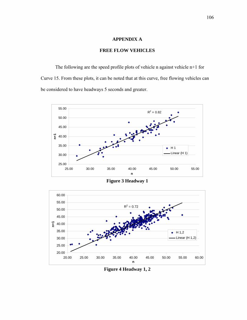
106

APPENDIX A

FREE FLOW VEHICLES

The following are the speed profile plots of vehicle n against vehicle n+1 for

Curve 15. From these plots, it can be noted that at this curve, free flowing vehicles can

be considered to have headways 5 seconds and greater.

R2 = 0.82

25.00

30.00

35.00

40.00

45.00

50.00

55.00

25.00 30.00 35.00 40.00 45.00 50.00 55.00n

n+1

H 1Linear (H 1)

Figure 3 Headway 1

R2 = 0.72

20.00

25.00

30.00

35.00

40.00

45.00

50.00

55.00

60.00

20.00 25.00 30.00 35.00 40.00 45.00 50.00 55.00 60.00n

n+1

H 1,2Linear (H 1,2)

Figure 4 Headway 1, 2

107

R2 = 0.71

20.00

25.00

30.00

35.00

40.00

45.00

50.00

55.00

60.00

20.00 30.00 40.00 50.00 60.00n

n+1

H 1,2,3Linear (H 1,2,3)

Figure 5 Headway 1, 2, 3

R2 = 0.62

20.0025.0030.00

35.0040.0045.0050.00

55.0060.00

20.00 30.00 40.00 50.00 60.00n

n+1

H 1,2,3,4Linear (H 1,2,3,4)

Figure 6 Headway 1, 2, 3, 4

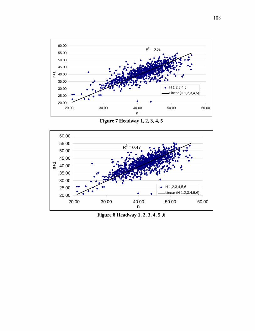
108

R2 = 0.52

20.00

25.00

30.00

35.00

40.00

45.00

50.00

55.00

60.00

20.00 30.00 40.00 50.00 60.00n

n+1

H 1,2,3,4,5Linear (H 1,2,3,4,5)

Figure 7 Headway 1, 2, 3, 4, 5

R2 = 0.47

20.00

25.0030.00

35.0040.00

45.00

50.0055.00

60.00

20.00 30.00 40.00 50.00 60.00n

n+1

H 1,2,3,4,5,6Linear (H 1,2,3,4,5,6)

Figure 8 Headway 1, 2, 3, 4, 5 ,6

109

APPENDIX B

REGRESSION

Figure 9 Scatter Plot of Speed vs. Square Root of Radius

110

Figure 10 Scatter Plot of Speed vs. Square Root of Superelevation

Figure 11 Scatter Plot of Speed vs. Posted Speed Limit

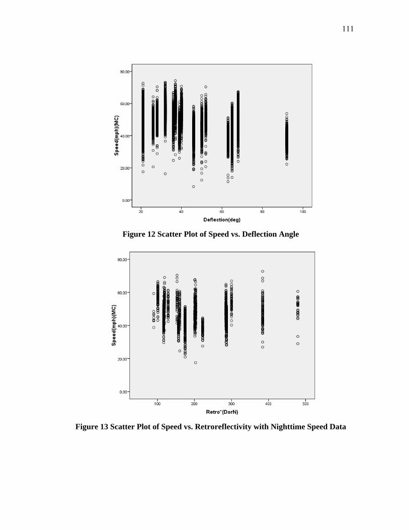
111

Figure 12 Scatter Plot of Speed vs. Deflection Angle

Figure 13 Scatter Plot of Speed vs. Retroreflectivity with Nighttime Speed Data

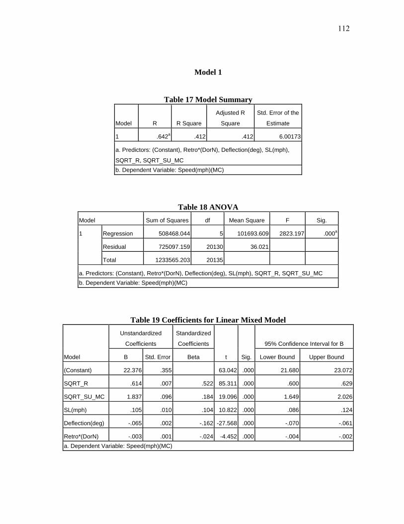
112

Model 1

Table 17 Model Summary

Model R R Square

Adjusted R

Square

Std. Error of the

Estimate

1 .642a .412 .412 6.00173

a. Predictors: (Constant), Retro*(DorN), Deflection(deg), SL(mph),

SQRT_R, SQRT_SU_MC b. Dependent Variable: Speed(mph)(MC)

Table 18 ANOVA Model Sum of Squares df Mean Square F Sig.

1 Regression 508468.044 5 101693.609 2823.197 .000a

Residual 725097.159 20130 36.021

Total 1233565.203 20135

a. Predictors: (Constant), Retro*(DorN), Deflection(deg), SL(mph), SQRT_R, SQRT_SU_MC b. Dependent Variable: Speed(mph)(MC)

Table 19 Coefficients for Linear Mixed Model

Model

Unstandardized

Coefficients

Standardized

Coefficients

t Sig.

95% Confidence Interval for B

B Std. Error Beta Lower Bound Upper Bound

(Constant) 22.376 .355 63.042 .000 21.680 23.072

SQRT_R .614 .007 .522 85.311 .000 .600 .629

SQRT_SU_MC 1.837 .096 .184 19.096 .000 1.649 2.026

SL(mph) .105 .010 .104 10.822 .000 .086 .124

Deflection(deg) -.065 .002 -.162 -27.568 .000 -.070 -.061

Retro*(DorN) -.003 .001 -.024 -4.452 .000 -.004 -.002a. Dependent Variable: Speed(mph)(MC)

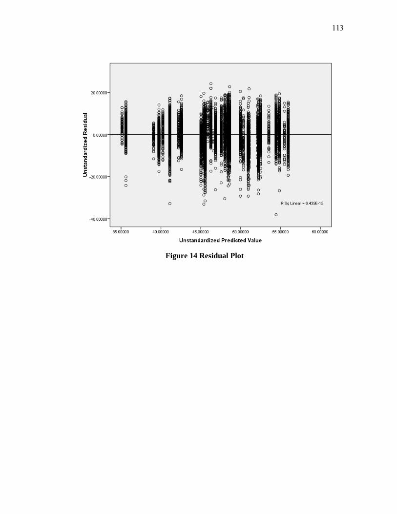
113

Figure 14 Residual Plot

114

Figure 15 Histogram

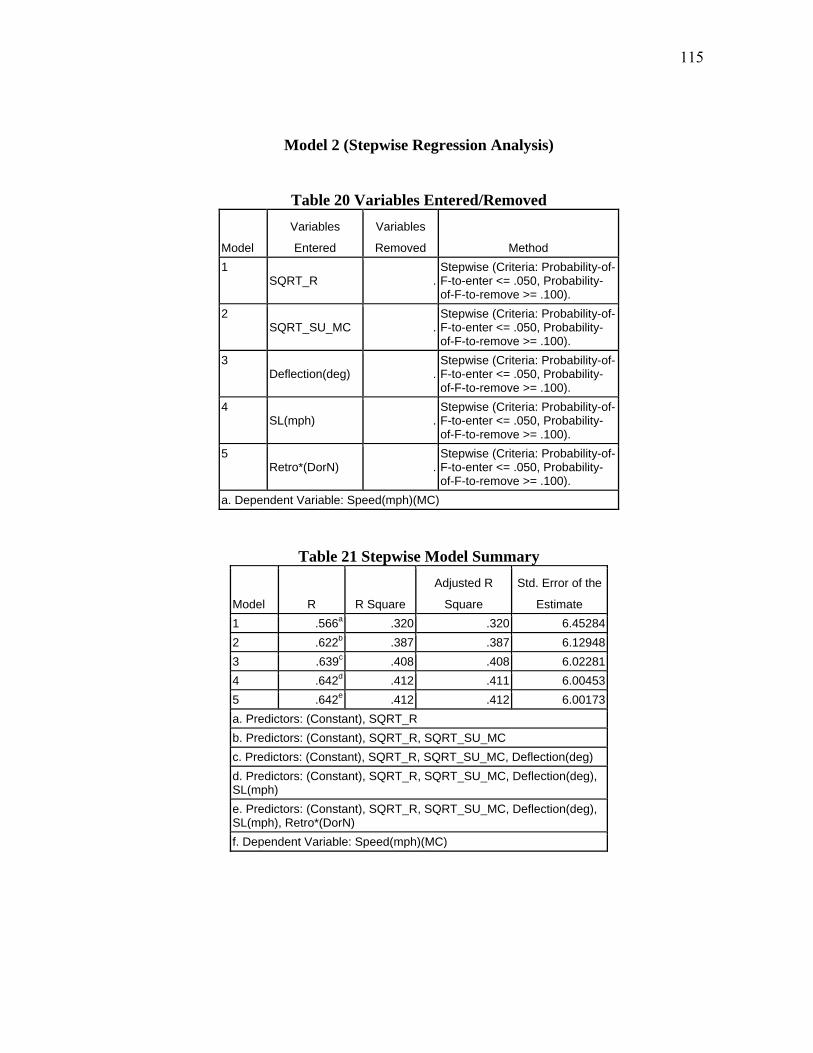
115

Model 2 (Stepwise Regression Analysis)

Table 20 Variables Entered/Removed

Model

Variables

Entered

Variables

Removed Method 1

SQRT_R .Stepwise (Criteria: Probability-of-F-to-enter <= .050, Probability-of-F-to-remove >= .100).

2 SQRT_SU_MC .

Stepwise (Criteria: Probability-of-F-to-enter <= .050, Probability-of-F-to-remove >= .100).

3 Deflection(deg) .


4 SL(mph) .


5 Retro*(DorN) .


a. Dependent Variable: Speed(mph)(MC)

Table 21 Stepwise Model Summary

Model R R Square

Adjusted R

Square

Std. Error of the

Estimate 1 .566a .320 .320 6.45284 2 .622b .387 .387 6.12948 3 .639c .408 .408 6.02281 4 .642d .412 .411 6.00453 5 .642e .412 .412 6.00173 a. Predictors: (Constant), SQRT_Rb. Predictors: (Constant), SQRT_R, SQRT_SU_MC c. Predictors: (Constant), SQRT_R, SQRT_SU_MC, Deflection(deg) d. Predictors: (Constant), SQRT_R, SQRT_SU_MC, Deflection(deg), SL(mph) e. Predictors: (Constant), SQRT_R, SQRT_SU_MC, Deflection(deg), SL(mph), Retro*(DorN) f. Dependent Variable: Speed(mph)(MC)

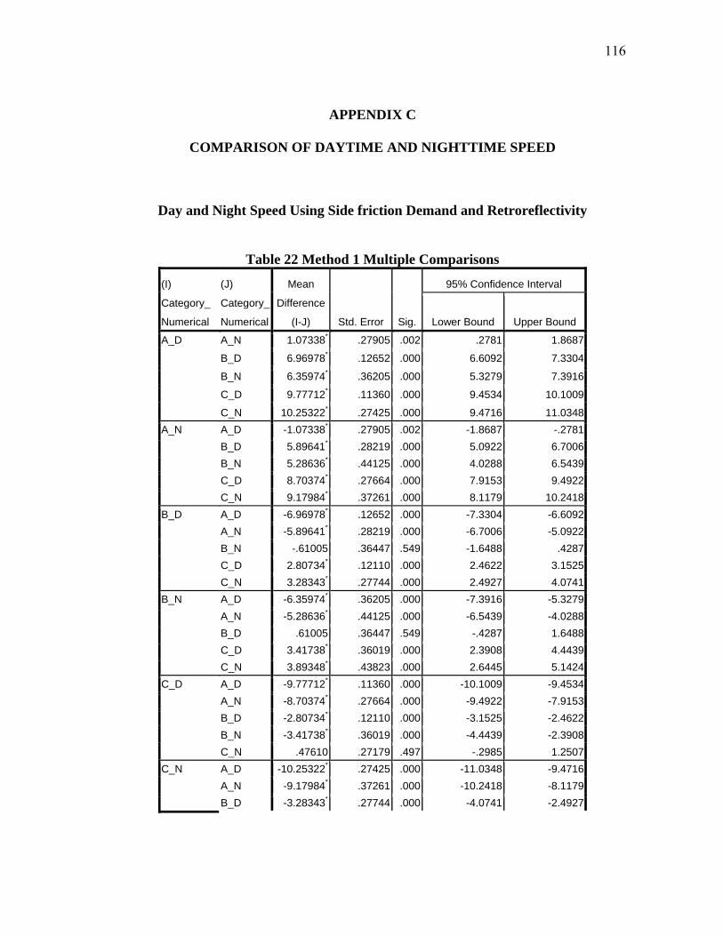
116

APPENDIX C

COMPARISON OF DAYTIME AND NIGHTTIME SPEED

Day and Night Speed Using Side friction Demand and Retroreflectivity

Table 22 Method 1 Multiple Comparisons

(I)

Category_

Numerical

(J)

Category_

Numerical

Mean

Difference

(I-J) Std. Error Sig.

95% Confidence Interval

Lower Bound Upper Bound

A_D A_N 1.07338* .27905 .002 .2781 1.8687

B_D 6.96978* .12652 .000 6.6092 7.3304

B_N 6.35974* .36205 .000 5.3279 7.3916

C_D 9.77712* .11360 .000 9.4534 10.1009

C_N 10.25322* .27425 .000 9.4716 11.0348A_N A_D -1.07338* .27905 .002 -1.8687 -.2781

B_D 5.89641* .28219 .000 5.0922 6.7006B_N 5.28636* .44125 .000 4.0288 6.5439C_D 8.70374* .27664 .000 7.9153 9.4922C_N 9.17984* .37261 .000 8.1179 10.2418

B_D A_D -6.96978* .12652 .000 -7.3304 -6.6092A_N -5.89641* .28219 .000 -6.7006 -5.0922B_N -.61005 .36447 .549 -1.6488 .4287C_D 2.80734* .12110 .000 2.4622 3.1525C_N 3.28343* .27744 .000 2.4927 4.0741

B_N A_D -6.35974* .36205 .000 -7.3916 -5.3279A_N -5.28636* .44125 .000 -6.5439 -4.0288B_D .61005 .36447 .549 -.4287 1.6488C_D 3.41738* .36019 .000 2.3908 4.4439C_N 3.89348* .43823 .000 2.6445 5.1424

C_D A_D -9.77712* .11360 .000 -10.1009 -9.4534A_N -8.70374* .27664 .000 -9.4922 -7.9153B_D -2.80734* .12110 .000 -3.1525 -2.4622B_N -3.41738* .36019 .000 -4.4439 -2.3908C_N .47610 .27179 .497 -.2985 1.2507

C_N A_D -10.25322* .27425 .000 -11.0348 -9.4716A_N -9.17984* .37261 .000 -10.2418 -8.1179B_D -3.28343* .27744 .000 -4.0741 -2.4927

117

B_N -3.89348* .43823 .000 -5.1424 -2.6445C_D -.47610 .27179 .497 -1.2507 .2985


(I)

Category_

Numerical

(J)

Category_

Numerical

Mean

Difference




A_D A_N 1.07338* .27914 .002 .2778 1.8689

B_D 6.96978* .12656 .000 6.6091 7.3305

B_N 6.35974* .36216 .000 5.3276 7.3919

C_D 9.15342* .11682 .000 8.8205 9.4864

C_N 9.64269* .29301 .000 8.8076 10.4778A_N A_D -1.07338* .27914 .002 -1.8689 -.2778

B_D 5.89641* .28228 .000 5.0919 6.7009B_N 5.28636* .44139 .000 4.0284 6.5443C_D 8.08004* .27805 .000 7.2876 8.8725C_N 8.56932* .38667 .000 7.4673 9.6713

B_D A_D -6.96978* .12656 .000 -7.3305 -6.6091A_N -5.89641* .28228 .000 -6.7009 -5.0919B_N -.61005 .36459 .550 -1.6491 .4290C_D 2.18363* .12414 .000 1.8298 2.5374C_N 2.67291* .29600 .000 1.8293 3.5165

B_N A_D -6.35974* .36216 .000 -7.3919 -5.3276A_N -5.28636* .44139 .000 -6.5443 -4.0284B_D .61005 .36459 .550 -.4290 1.6491C_D 2.79368* .36132 .000 1.7639 3.8234C_N 3.28296* .45029 .000 1.9996 4.5663

C_D A_D -9.15342* .11682 .000 -9.4864 -8.8205A_N -8.08004* .27805 .000 -8.8725 -7.2876B_D -2.18363* .12414 .000 -2.5374 -1.8298B_N -2.79368* .36132 .000 -3.8234 -1.7639C_N .48928 .29197 .548 -.3428 1.3214

C_N A_D -9.64269* .29301 .000 -10.4778 -8.8076A_N -8.56932* .38667 .000 -9.6713 -7.4673B_D -2.67291* .29600 .000 -3.5165 -1.8293B_N -3.28296* .45029 .000 -4.5663 -1.9996C_D -.48928 .29197 .548 -1.3214 .3428

118


(I)

Category_

Numerical

(J)

Category_

Numerical

Mean

Difference




A_D A_N -.10721 .23902 .970 -.7213 .5069

B_D 6.05200* .11049 .000 5.7681 6.3359

B_N 6.54128* .31041 .000 5.7438 7.3388A_N A_D .10721 .23902 .970 -.5069 .7213

B_D 6.15922* .24519 .000 5.5293 6.7892B_N 6.64850* .37982 .000 5.6726 7.6244

B_D A_D -6.05200* .11049 .000 -6.3359 -5.7681A_N -6.15922* .24519 .000 -6.7892 -5.5293B_N .48928 .31519 .406 -.3205 1.2991

B_N A_D -6.54128* .31041 .000 -7.3388 -5.7438A_N -6.64850* .37982 .000 -7.6244 -5.6726B_D -.48928 .31519 .406 -1.2991 .3205


(I)

Category_

Numerical

(J)

Category_

Numerical

Mean

Difference




A_D A_N -.68932 .47163 .689 -2.0335 .6548

B_D 6.75930* .14625 .000 6.3425 7.1761

B_N 6.53516* .27641 .000 5.7474 7.3229

C_D 11.05652* .15037 .000 10.6280 11.4851

C_N 11.54580* .31249 .000 10.6552 12.4364A_N A_D .68932 .47163 .689 -.6548 2.0335

B_D 7.44862* .46059 .000 6.1359 8.7613B_N 7.22448* .51688 .000 5.7514 8.6976C_D 11.74585* .46192 .000 10.4294 13.0623C_N 12.23513* .53704 .000 10.7046 13.7657

B_D A_D -6.75930* .14625 .000 -7.1761 -6.3425A_N -7.44862* .46059 .000 -8.7613 -6.1359B_N -.22414 .25714 .953 -.9570 .5087C_D 4.29723* .11104 .000 3.9808 4.6137C_N 4.78651* .29558 .000 3.9441 5.6289

B_N A_D -6.53516* .27641 .000 -7.3229 -5.7474A_N -7.22448* .51688 .000 -8.6976 -5.7514B_D .22414 .25714 .953 -.5087 .9570

119

C_D 4.52137* .25951 .000 3.7818 5.2610C_N 5.01065* .37734 .000 3.9352 6.0861

C_D A_D -11.05652* .15037 .000 -11.4851 -10.6280A_N -11.74585* .46192 .000 -13.0623 -10.4294B_D -4.29723* .11104 .000 -4.6137 -3.9808B_N -4.52137* .25951 .000 -5.2610 -3.7818C_N .48928 .29764 .569 -.3590 1.3376

C_N A_D -11.54580* .31249 .000 -12.4364 -10.6552A_N -12.23513* .53704 .000 -13.7657 -10.7046B_D -4.78651* .29558 .000 -5.6289 -3.9441B_N -5.01065* .37734 .000 -6.0861 -3.9352C_D -.48928 .29764 .569 -1.3376 .3590


(I)

Category_

Numerical

(J)

Category_

Numerical

Mean

Difference (I-J)

Std.

Error Sig.



A_D A_N -1.21073 .53324 .206 -2.7306 .3091

B_D 6.64613* .16402 .000 6.1786 7.1136

B_N 6.46323* .32290 .000 5.5429 7.3836

C_D 9.25758* .19383 .000 8.7051 9.8100

C_N 8.62264* .48499 .000 7.2403 10.0050A_N A_D 1.21073 .53324 .206 -.3091 2.7306

B_D 7.85686* .52261 .000 6.3673 9.3464B_N 7.67396* .59201 .000 5.9866 9.3613C_D 10.46831* .53272 .000 8.9500 11.9866C_N 9.83336* .69386 .000 7.8558 11.8110

B_D A_D -6.64613* .16402 .000 -7.1136 -6.1786A_N -7.85686* .52261 .000 -9.3464 -6.3673B_N -.18290 .30502 .991 -1.0523 .6865C_D 2.61145* .16231 .000 2.1488 3.0741C_N 1.97651* .47328 .000 .6276 3.3254

B_N A_D -6.46323* .32290 .000 -7.3836 -5.5429A_N -7.67396* .59201 .000 -9.3613 -5.9866B_D .18290 .30502 .991 -.6865 1.0523C_D 2.79435* .32203 .000 1.8765 3.7122C_N 2.15941* .54896 .001 .5948 3.7240

C_D A_D -9.25758* .19383 .000 -9.8100 -8.7051A_N -10.46831* .53272 .000 -11.9866 -8.9500B_D -2.61145* .16231 .000 -3.0741 -2.1488

120

B_N -2.79435* .32203 .000 -3.7122 -1.8765C_N -.63494 .48442 .779 -2.0156 .7457

C_N A_D -8.62264* .48499 .000 -10.0050 -7.2403A_N -9.83336* .69386 .000 -11.8110 -7.8558B_D -1.97651* .47328 .000 -3.3254 -.6276B_N -2.15941* .54896 .001 -3.7240 -.5948C_D .63494 .48442 .779 -.7457 2.0156


(I)

Category_

Numerical

(J)

Category_

Numerical

Mean

Difference (I-J)

Std.

Error Sig.



A_D A_N -1.21073 .52774 .393 -2.8805 .4591

B_D 4.76811* .19043 .000 4.1656 5.3706

B_N 4.67153* .45568 .000 3.2297 6.1133

C_D 6.64613* .16233 .000 6.1325 7.1598

C_N 6.46323* .31957 .000 5.4521 7.4744

D_D 9.25758* .19183 .000 8.6506 9.8645

D_N 8.62264* .47999 .000 7.1039 10.1413

E_D 11.69734* .17228 .000 11.1522 12.2425

E_N 12.95816* .39290 .000 11.7150 14.2013A_N A_D 1.21073 .52774 .393 -.4591 2.8805

B_D 5.97884* .52671 .000 4.3123 7.6454B_N 5.88226* .66993 .000 3.7626 8.0019C_D 7.85686* .51722 .000 6.2204 9.4934C_N 7.67396* .58590 .000 5.8201 9.5278D_D 10.46831* .52722 .000 8.8002 12.1365D_N 9.83336* .68669 .000 7.6606 12.0061E_D 12.90807* .52043 .000 11.2614 14.5547E_N 14.16889* .62891 .000 12.1790 16.1588

B_D A_D -4.76811* .19043 .000 -5.3706 -4.1656A_N -5.97884* .52671 .000 -7.6454 -4.3123B_N -.09658 .45449 1.000 -1.5346 1.3414C_D 1.87801* .15896 .000 1.3751 2.3810C_N 1.69512* .31787 .000 .6894 2.7009D_D 4.48947* .18898 .000 3.8915 5.0874D_N 3.85452* .47886 .000 2.3394 5.3697E_D 6.92923* .16911 .000 6.3942 7.4643

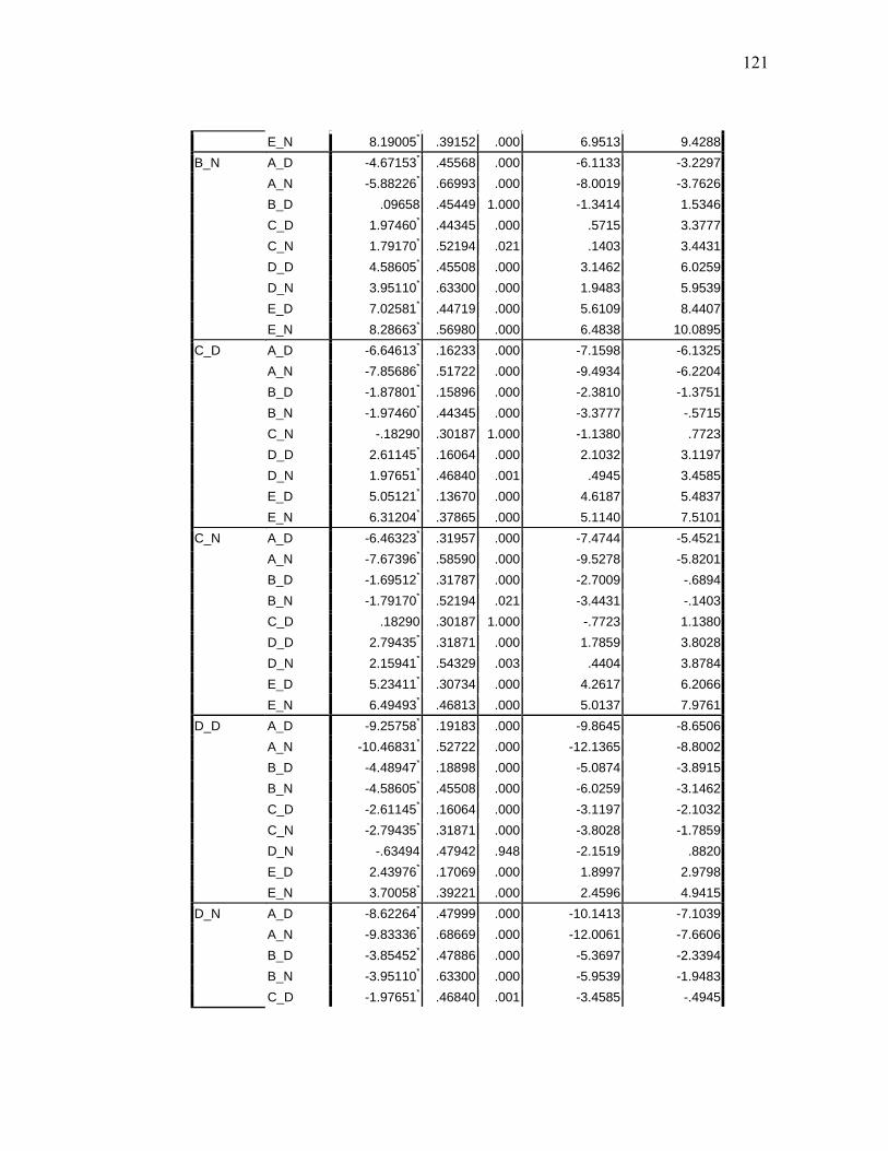
121

E_N 8.19005* .39152 .000 6.9513 9.4288B_N A_D -4.67153* .45568 .000 -6.1133 -3.2297

A_N -5.88226* .66993 .000 -8.0019 -3.7626B_D .09658 .45449 1.000 -1.3414 1.5346C_D 1.97460* .44345 .000 .5715 3.3777C_N 1.79170* .52194 .021 .1403 3.4431D_D 4.58605* .45508 .000 3.1462 6.0259D_N 3.95110* .63300 .000 1.9483 5.9539E_D 7.02581* .44719 .000 5.6109 8.4407E_N 8.28663* .56980 .000 6.4838 10.0895

C_D A_D -6.64613* .16233 .000 -7.1598 -6.1325A_N -7.85686* .51722 .000 -9.4934 -6.2204B_D -1.87801* .15896 .000 -2.3810 -1.3751B_N -1.97460* .44345 .000 -3.3777 -.5715C_N -.18290 .30187 1.000 -1.1380 .7723D_D 2.61145* .16064 .000 2.1032 3.1197D_N 1.97651* .46840 .001 .4945 3.4585E_D 5.05121* .13670 .000 4.6187 5.4837E_N 6.31204* .37865 .000 5.1140 7.5101

C_N A_D -6.46323* .31957 .000 -7.4744 -5.4521A_N -7.67396* .58590 .000 -9.5278 -5.8201B_D -1.69512* .31787 .000 -2.7009 -.6894B_N -1.79170* .52194 .021 -3.4431 -.1403C_D .18290 .30187 1.000 -.7723 1.1380D_D 2.79435* .31871 .000 1.7859 3.8028D_N 2.15941* .54329 .003 .4404 3.8784E_D 5.23411* .30734 .000 4.2617 6.2066E_N 6.49493* .46813 .000 5.0137 7.9761

D_D A_D -9.25758* .19183 .000 -9.8645 -8.6506A_N -10.46831* .52722 .000 -12.1365 -8.8002B_D -4.48947* .18898 .000 -5.0874 -3.8915B_N -4.58605* .45508 .000 -6.0259 -3.1462C_D -2.61145* .16064 .000 -3.1197 -2.1032C_N -2.79435* .31871 .000 -3.8028 -1.7859D_N -.63494 .47942 .948 -2.1519 .8820E_D 2.43976* .17069 .000 1.8997 2.9798E_N 3.70058* .39221 .000 2.4596 4.9415

D_N A_D -8.62264* .47999 .000 -10.1413 -7.1039A_N -9.83336* .68669 .000 -12.0061 -7.6606B_D -3.85452* .47886 .000 -5.3697 -2.3394B_N -3.95110* .63300 .000 -5.9539 -1.9483C_D -1.97651* .46840 .001 -3.4585 -.4945

122

C_N -2.15941* .54329 .003 -3.8784 -.4404D_D .63494 .47942 .948 -.8820 2.1519E_D 3.07470* .47194 .000 1.5815 4.5679E_N 4.33553* .58942 .000 2.4706 6.2005

E_D A_D -11.69734* .17228 .000 -12.2425 -11.1522A_N -12.90807* .52043 .000 -14.5547 -11.2614B_D -6.92923* .16911 .000 -7.4643 -6.3942B_N -7.02581* .44719 .000 -8.4407 -5.6109C_D -5.05121* .13670 .000 -5.4837 -4.6187C_N -5.23411* .30734 .000 -6.2066 -4.2617D_D -2.43976* .17069 .000 -2.9798 -1.8997D_N -3.07470* .47194 .000 -4.5679 -1.5815E_N 1.26083* .38303 .034 .0489 2.4727

E_N A_D -12.95816* .39290 .000 -14.2013 -11.7150A_N -14.16889* .62891 .000 -16.1588 -12.1790B_D -8.19005* .39152 .000 -9.4288 -6.9513B_N -8.28663* .56980 .000 -10.0895 -6.4838C_D -6.31204* .37865 .000 -7.5101 -5.1140C_N -6.49493* .46813 .000 -7.9761 -5.0137D_D -3.70058* .39221 .000 -4.9415 -2.4596D_N -4.33553* .58942 .000 -6.2005 -2.4706E_D -1.26083* .38303 .034 -2.4727 -.0489

123

Day and Night Speed Using Radius and Retroreflectivity


(I)

Category_

Numerical

(J)

Category_

Numerical

Mean Difference




A_D A_N .48928 .29054 .698 -.3914 1.3700

B_D .23067 .13157 .652 -.1681 .6295

B_N -.29500 .37686 .994 -1.4373 .8473

C_D -11.05652* .14679 .000 -11.5015 -10.6116

C_N -11.74585* .45090 .000 -13.1126 -10.3791

D_D -6.21612* .12262 .000 -6.5878 -5.8444

D_N -5.53680* .30028 .000 -6.4470 -4.6266A_N A_D -.48928 .29054 .698 -1.3700 .3914

B_D -.25861 .29801 .989 -1.1620 .6447B_N -.78428 .46209 .689 -2.1850 .6164C_D -11.54580* .30504 .000 -12.4704 -10.6212C_N -12.23513* .52422 .000 -13.8242 -10.6461D_D -6.70540* .29417 .000 -7.5971 -5.8137D_N -6.02608* .40208 .000 -7.2449 -4.8073

B_D A_D -.23067 .13157 .652 -.6295 .1681A_N .25861 .29801 .989 -.6447 1.1620B_N -.52566 .38265 .869 -1.6856 .6342C_D -11.28719* .16107 .000 -11.7754 -10.7990C_N -11.97651* .45575 .000 -13.3580 -10.5951D_D -6.44678* .13940 .000 -6.8693 -6.0242D_N -5.76747* .30751 .000 -6.6996 -4.8353

B_N A_D .29500 .37686 .994 -.8473 1.4373A_N .78428 .46209 .689 -.6164 2.1850B_D .52566 .38265 .869 -.6342 1.6856C_D -10.76153* .38815 .000 -11.9381 -9.5850C_N -11.45085* .57656 .000 -13.1985 -9.7032D_D -5.92112* .37967 .000 -7.0720 -4.7703D_N -5.24180* .46827 .000 -6.6612 -3.8224

C_D A_D 11.05652* .14679 .000 10.6116 11.5015A_N 11.54580* .30504 .000 10.6212 12.4704B_D 11.28719* .16107 .000 10.7990 11.7754B_N 10.76153* .38815 .000 9.5850 11.9381C_N -.68932 .46037 .809 -2.0848 .7062D_D 4.84041* .15385 .000 4.3741 5.3067

124

D_N 5.51972* .31432 .000 4.5669 6.4725C_N A_D 11.74585* .45090 .000 10.3791 13.1126

A_N 12.23513* .52422 .000 10.6461 13.8242B_D 11.97651* .45575 .000 10.5951 13.3580B_N 11.45085* .57656 .000 9.7032 13.1985C_D .68932 .46037 .809 -.7062 2.0848D_D 5.52973* .45325 .000 4.1559 6.9036D_N 6.20905* .52968 .000 4.6035 7.8146

D_D A_D 6.21612* .12262 .000 5.8444 6.5878A_N 6.70540* .29417 .000 5.8137 7.5971B_D 6.44678* .13940 .000 6.0242 6.8693B_N 5.92112* .37967 .000 4.7703 7.0720C_D -4.84041* .15385 .000 -5.3067 -4.3741C_N -5.52973* .45325 .000 -6.9036 -4.1559D_N .67932 .30379 .330 -.2415 1.6002

D_N A_D 5.53680* .30028 .000 4.6266 6.4470A_N 6.02608* .40208 .000 4.8073 7.2449B_D 5.76747* .30751 .000 4.8353 6.6996B_N 5.24180* .46827 .000 3.8224 6.6612C_D -5.51972* .31432 .000 -6.4725 -4.5669C_N -6.20905* .52968 .000 -7.8146 -4.6035D_D -.67932 .30379 .330 -1.6002 .2415


(I)

Category_

Numerical

(J)

Category_

Numerical

Mean Difference




A_D A_N -.63494 .43211 .824 -1.9449 .6750

B_D 3.83485* .18799 .000 3.2650 4.4047

B_N 3.51036* .57879 .000 1.7558 5.2649

C_D -9.25758* .17290 .000 -9.7817 -8.7334

C_N -10.46831* .47520 .000 -11.9088 -9.0278

D_D -5.40785* .15385 .000 -5.8742 -4.9415

D_N -4.48728* .31737 .000 -5.4494 -3.5252A_N A_D .63494 .43211 .824 -.6750 1.9449

B_D 4.46979* .43888 .000 3.1394 5.8002B_N 4.14530* .70162 .000 2.0184 6.2722C_D -8.62264* .43263 .000 -9.9341 -7.3112C_N -9.83336* .61894 .000 -11.7096 -7.9571

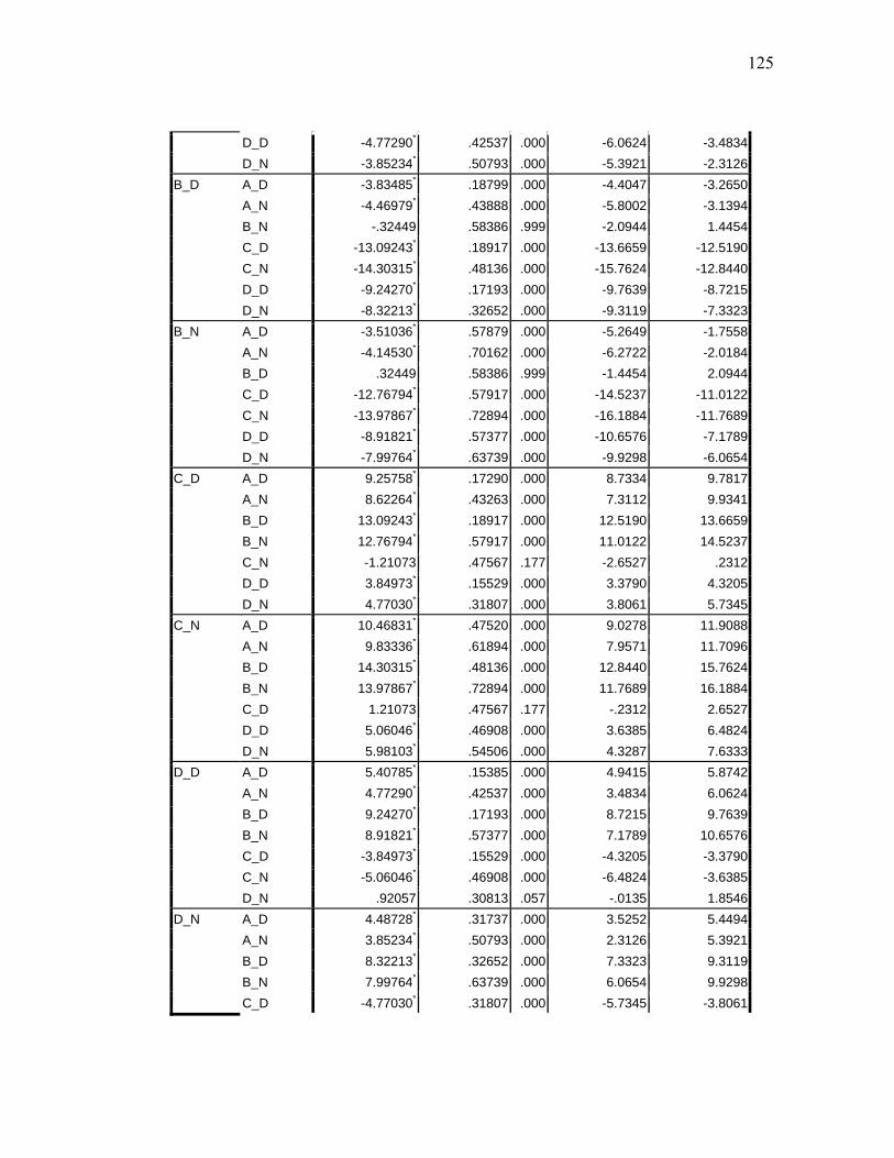
125

D_D -4.77290* .42537 .000 -6.0624 -3.4834D_N -3.85234* .50793 .000 -5.3921 -2.3126

B_D A_D -3.83485* .18799 .000 -4.4047 -3.2650A_N -4.46979* .43888 .000 -5.8002 -3.1394B_N -.32449 .58386 .999 -2.0944 1.4454C_D -13.09243* .18917 .000 -13.6659 -12.5190C_N -14.30315* .48136 .000 -15.7624 -12.8440D_D -9.24270* .17193 .000 -9.7639 -8.7215D_N -8.32213* .32652 .000 -9.3119 -7.3323

B_N A_D -3.51036* .57879 .000 -5.2649 -1.7558A_N -4.14530* .70162 .000 -6.2722 -2.0184B_D .32449 .58386 .999 -1.4454 2.0944C_D -12.76794* .57917 .000 -14.5237 -11.0122C_N -13.97867* .72894 .000 -16.1884 -11.7689D_D -8.91821* .57377 .000 -10.6576 -7.1789D_N -7.99764* .63739 .000 -9.9298 -6.0654

C_D A_D 9.25758* .17290 .000 8.7334 9.7817A_N 8.62264* .43263 .000 7.3112 9.9341B_D 13.09243* .18917 .000 12.5190 13.6659B_N 12.76794* .57917 .000 11.0122 14.5237C_N -1.21073 .47567 .177 -2.6527 .2312D_D 3.84973* .15529 .000 3.3790 4.3205D_N 4.77030* .31807 .000 3.8061 5.7345

C_N A_D 10.46831* .47520 .000 9.0278 11.9088A_N 9.83336* .61894 .000 7.9571 11.7096B_D 14.30315* .48136 .000 12.8440 15.7624B_N 13.97867* .72894 .000 11.7689 16.1884C_D 1.21073 .47567 .177 -.2312 2.6527D_D 5.06046* .46908 .000 3.6385 6.4824D_N 5.98103* .54506 .000 4.3287 7.6333

D_D A_D 5.40785* .15385 .000 4.9415 5.8742A_N 4.77290* .42537 .000 3.4834 6.0624B_D 9.24270* .17193 .000 8.7215 9.7639B_N 8.91821* .57377 .000 7.1789 10.6576C_D -3.84973* .15529 .000 -4.3205 -3.3790C_N -5.06046* .46908 .000 -6.4824 -3.6385D_N .92057 .30813 .057 -.0135 1.8546

D_N A_D 4.48728* .31737 .000 3.5252 5.4494A_N 3.85234* .50793 .000 2.3126 5.3921B_D 8.32213* .32652 .000 7.3323 9.3119B_N 7.99764* .63739 .000 6.0654 9.9298C_D -4.77030* .31807 .000 -5.7345 -3.8061

126

C_N -5.98103* .54506 .000 -7.6333 -4.3287D_D -.92057 .30813 .057 -1.8546 .0135

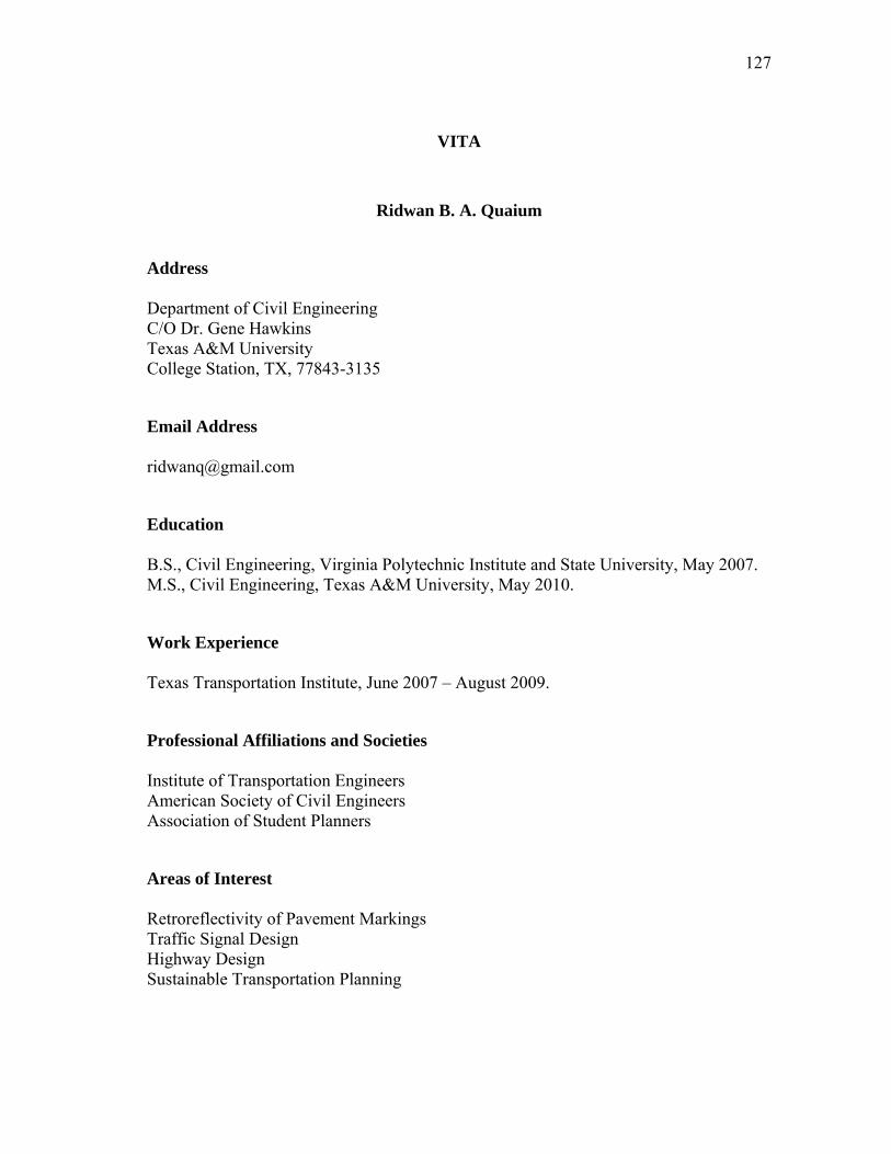
127

VITA

Ridwan B. A. Quaium

Address

Department of Civil Engineering C/O Dr. Gene Hawkins Texas A&M University College Station, TX, 77843-3135

Email Address

[email protected]

Education

B.S., Civil Engineering, Virginia Polytechnic Institute and State University, May 2007. M.S., Civil Engineering, Texas A&M University, May 2010.

Work Experience

Texas Transportation Institute, June 2007 – August 2009.

Professional Affiliations and Societies

Institute of Transportation Engineers American Society of Civil Engineers Association of Student Planners

Areas of Interest

Retroreflectivity of Pavement Markings Traffic Signal Design Highway Design Sustainable Transportation Planning

Documents

A COMPARISON OF VEHICLE SPEED AT DAY AND NIGHT AT RURALceprofs.civil.tamu.edu/ghawkins/Thesis_Final/QUAIUM-THESIS.pdf · A Comparison of Vehicle Speed at Day and Night at Rural