A Comparison of Transects and Point Counts in Oak-pine ... · A COMPARISON OF TRANSECTS AND POINT COUNTS IN OAK-PINE WOODLANDS OF CALIFORNIA JARED VERNER AND LYMAN V. RITTER ABSTRACT.-Transects

The Condor 87:47-68 0 The Cooper Ornithological Society 1985

A COMPARISON OF TRANSECTS AND POINT COUNTS IN OAK-PINE WOODLANDS OF CALIFORNIA

JARED VERNER AND

LYMAN V. RITTER

ABSTRACT.-Transects and point counts were compared as methods for measuring species richness, relative abundance, and density of birds in oak-pine woodlands of central California. Efficiency of the two methods for measuring species richness or giving total counts varied with study design and season. We recommend point counts over transects for most studies in which results of these methods are suitable. Frequency is a measure of relative abundance that should be used only with due caution for its limitations. Density estimates are probably superior to total counts for indexing relative abundance, but they are limited because: (1) the small sample sizes attained in most studies permit density estimation for only a small percentage of the species detected; and (2) available evidence challenges assumptions that density estimates by transects or point counts are acceptably accurate.

Much field research on birds requires estimations of abundance. Commonly, however, researchers fail to evaluate the scale of abundance needed to answer their particular question, instead seeking data on a scale more detailed than the study requires. Measures of abundance give information at four scales (def- initions not fully in agreement with those used by statisticians): (1) a “nominal scale” requires information only about occurrence; (2) an “ordinal scale” requires sufficient information to rank species in the correct order of abundance; (3) a “ratio scale” requires equivalent estimates of abundance (either bias must be small or in constant proportion to population density for each species); and (4) an “absolute scale” requires accurate, i.e., unbiased, estimates of abundance suitable for calculating density. Information at a nominal scale is sufficient to express abundance in terms of frequency-the proportion of counts in which a species is detected. Simple counts unadjusted for differences in area have been used to rank species in order of abundance (ordinal scale), although this assumes that all species are equally detectable. Population trends can be detected by information on a ratio scale, but some studies (e.g., trophic dynamics) require estimates of species’ densities (absolute scale). In this case, comparisons between species, or within species between habitats, require methods that reasonably accurately estimate density.

This paper compares three variants each of transects and point counts as methods to measure abundance at nominal, ordinal, ratio, or absolute scales. For transects these are (1) strip

transects (fixed limits for all species), (2) line transects with variable limits, by species (Em- len 1971, 1977; Bumham et al. 1980), and (3) line transects without limits (total counts; not suited for estimating densities). Similarly, for point counts they are (1) plot counts (fixed radii for all species), (2) point counts with variable radii, by species (Reynolds et al. 1980), and (3) point counts with unlimited radii (total counts). Our ability to make these comparisons is limited by the same flaw that mars most other comparisons found in the literature: methods of estimation are compared with one another, not with an absolute standard. .Uthough we cannot measure the accuracy of these methods, we can infer much about their accuracy through a variety of comparisons.

STUDY AREA

Field work was done at the San Joaquin Ex- perimental Range, Madera County, California (Fig. 1). The Experimental Range (hereafter “SJER”), managed by the Forest Service, U.S. Department of Agriculture, occupies an area of about 1,875 ha in oak and oak-pine woodlands in the western foothills of the Sierra Ne- vada, at 2 15-520 m elevation. The climate at SJER is characterized by cool, wet winters and hot, dry summers. Annual precipitation av- erages 48.6 cm (43-year mean, 193%1977), with most falling as rain from November through March.

Two study plots, each 660 m by 300 m (19.8 ha), were selected from aerial photographs so as to have comparable relief and tree canopy cover of vegetation characteristic of the blue

[471

48 JARED VERNER AND LYMAN V. RITTER

SJER

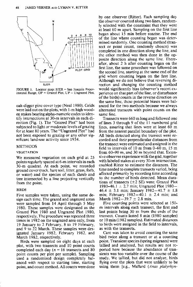
FIGURE 1. Locator map: SJER = San Joaquin Exper- imental Range, GP = Grazed Plot, UP = Ungrazed Plot.

oak-digger pine cover type (Neal 1980). Grids were laid out on the plots, with 1 -m high wood- en stakes bearing alpha-numeric codes to identify intersections at 30-m intervals in each direction (Fig. 1). The “Grazed Plot” had been subjected to light or moderate levels of grazing for at least 80 years. The “Ungrazed Plot” had not been exposed to grazing or any other significant land-use activity since 1934.

METHODS

VEGETATION

We measured vegetation on each grid at 25 points regularly spaced at 6-m intervals in each 30-m quadrat. At each point, we recorded ground cover (rock, bare soil, litter, grass, forb, or water) and the species of each shrub and tree intersected by a line projecting vertically from the point.

BIRDS

Five samples were taken, using the same design each time. The grazed and ungrazed areas were sampled from 14 April through 5 May 1980, These samples were designated as the Grazed Plot 1980 and Ungrazed Plot 1980, respectively. The procedure was repeated three times in 1982 on the ungrazed area only, from 19 January to 2 February, 8 to 19 February, and 9 to 22 March. These samples were designated January 1982, February 1982, and March 1982, respectively.

Birds were sampled on eight days at each plot, with two transects and 10 point counts completed each day (~1 = 16 transects and 80 point counts per plot per sample). Sampling used a randomized design completely bal- anced with respect to starting time, starting point, and count method. All counts were done

by one observer (Ritter). Each sampling day the observer counted along two lines, randomly selected with the constraint that they were at least 60 m apart. Sampling on the first line began about 15 min before sunrise. The end of the line where counting began was determined randomly. One counting method (transect or point count, randomly chosen) was completed in one direction along the line, and the other method was then done in the op- posite direction along the same line. There- after, about 2 h after counting began on the first line, the same procedure was followed on the second line, starting at the same end of the grid where counting began on the first line. Although we do not believe that reversing direction and changing the counting method would significantly bias (observer’s recent experience on that part of the line, or disturbance of the birds) counts in the reverse direction on the same line, these potential biases were bal- anced for the two methods because we always alternated transects with point counts on the same line.

Transects were 660 m long and followed one of lines 3 through 9 of the 11 numbered grid lines, assuring that lines were at least 60 m from the nearest parallel boundary of the plot. All birds detected along the transect were recorded and their perpendicular distances from the transect were estimated and assigned in the field to intervals of 10 m from O-60 m, 15 m from 60-90 m, and 30 m beyond that. Exten- sive observer experience with the grid, together with labeled stakes at every 30-m intersection, enabled Ritter to estimate the distances. The time needed to complete transects varied, being affected primarily by recording time according to the number of birds detected. Mean dura- tions of transects (+2 SE) were: Grazed Plot 1980-46.1 f 2.7 min; Ungrazed Plot 1980- 46.4 -t 3.1 min; January 1982-41.7 + 1.8 min; February 1982-40.1 f 2.4 min; and March 1982-39.7 & 2.8 min.

Five counting points were selected at 150- m intervals along each transect, the first and last points being 30 m from the ends of the transect. Counts lasted 8 min (1980 samples) or 10 min (1982 samples). Estimated distances to birds were assigned in the field to intervals, as with the transects.

Care was taken to avoid counting the same bird twice along a transect or at a counting point. Transient species (spring migrants) were tallied and analyzed, but results are not reported here because the abundance of tran- sients was too variable over the course of the study. We tallied, but did not analyze, birds flying over the plots that were unlikely to be using them [e.g., Mallard (Anas platyrhyn-

COMPARING TRANSECTS AND POINT COUNTS 49

chos), Killdeer (Charadrius vociferus), Amer- ican Crow (Corvus brachyrhynchos), and Red- winged Blackbird (Agelaius phoeniceus)].

ANALYSIS

Unless otherwise noted, we used an alpha level of 0.05 in all tests of significance. The effects of study design on counts, resulting from differences in (1) starting time along each line, (2) end of the transect where counting began, (3) method used (points or transects), and (4) plot (grazed or ungrazed), were tested by analysis of variance (ANOVA) applied to total counts of species with sufficiently large sample sizes (n = 40+, summed over all counts; see Burn- ham et al. 1980:33).

Because one could use a percentage of the assemblage of species available as a standard to identify a sufficient sampling effort when measuring species richness, we attempted to define the assemblage appropriate to each sample. We identified three sorts of assemblages: (1) nesting assemblages for each of the 1980 samples, using the summation of all species found nesting on each plot during the preced- ing 5-year period; (2) total assemblages for the 1980 samples, using nesting assemblages plus additional species known to nest near enough to the plots to include them within their ter- ritories or home ranges; and (3) total assemblages for the 1982 samples, using (a) general knowledge about the avifauna of oak-pine woodlands in the west-central foothills of the Sierra Nevada, (b) the total sampling effort by point and transect counts on each plot for each time period during this study, and (c) knowledge derived from other extensive field work on the plots during comparable time periods in other years. We recognize, of course, that such efforts must fall short of the goal of de- fining total assemblages, because birds are so mobile.

Bootstrap estimations (Efron and Gong 1983) were performed to plot species accumulation curves with increasing numbers of points and transects counted. Each point on the estimated curves represents the mean for all possible combinations of samples of a given size, taken with replacement from the complete set of actual samples.

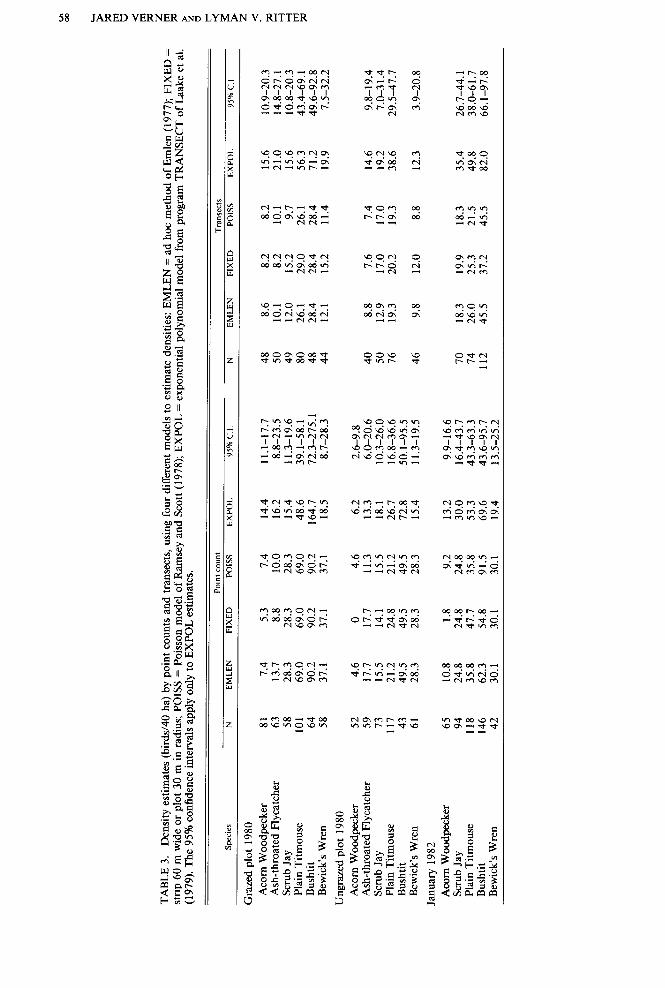
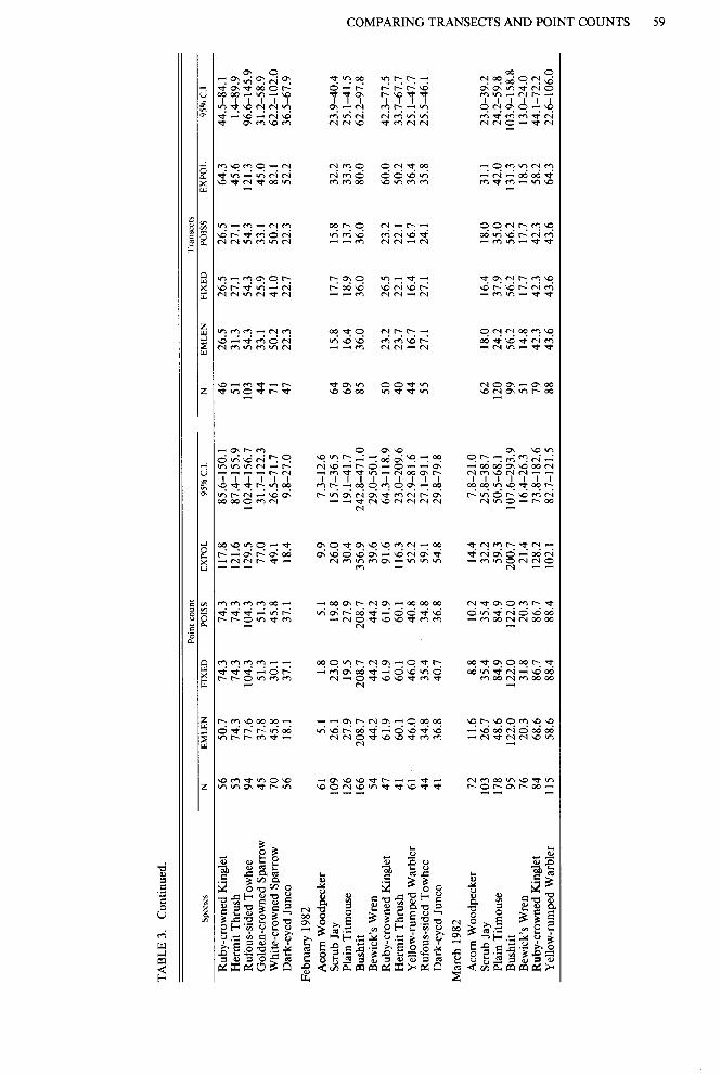
Total counts (sum of all individuals detected in all transects or point counts in a given sample) and frequencies (number of transects or point counts with the species detected divided by the number of counts) were determined for all species detected in each assemblage, and densities were computed by four estimators for species detected in sufficient numbers. Esti- mators were (1) FIXED: strip transects 60 m wide, or circular plots 60 m in diameter; (2)

EMLEN: based on Emlen’s (1977) ad hoc model; (3) POISS: based on Ramsey and Scott’s (1978) method assuming Poisson scattering of counts, and using Program CIRPLOT developed in our laboratory by C. J. Evans and M. R. Bryan; (4) EXPOL: based on the exponen- tial polynomial model discussed by Burnham et al. (1980) using Program TRANSECT (Laake et al. 1979). FIXED was chosen because it has been widely used in studies of bird densities and because its assumptions are clearcut. The EMLEN estimator was selected for comparative purposes with POISS because it has been widely used by ornithologists. The POISS estimator, although lacking a clear inferential basis, has been introduced only re- cently and offers a less subjective method for selecting the basal distance to be used for each species. (The “basal region,” as used by Emlen [1971, 19771 and Ramsey and Scott [1981], is that area sampled within which the observer is believed to detect all individuals of a given species. “Basal distance” is used here to des- ignate the distance to the outer limit of the basal region-a radius in point counts; a perpendicular distance from the line in line transects. Ideally it can be identified by an inflec- tion point in detections with distance from the observer.) EXPOL was selected because it has a clear inferential basis and because it has been shown to be more robust to movement by animals than other models tested by Burnham et al. (1980). Densities were also estimated by the Fourier series estimator developed by Burnham et al. (1980), but most results are not reported here because EXPOL was judged to be better. Many additional estimators could have been used as well (see Robinette et al. 1974, and Tilghman and Rusch 198 l), but Burnham et al. (1980) judged them to be flawed in one way or another. The method of Jarvinen and Vaisanen (1975) assumes that detectability of birds decreases linearly with distance from the transect. Our results clearly did not meet this assumption.

We estimated densities only for those species with total counts of 40 or more individuals in a given sample period. This met the minimum standard recommended by Bumham et al. (1980), but not their preferred standard of 60- 80 individuals per sample. Densities of species with lower counts have been estimated by some observers by using basal distances of other species considered to be similarly detectable (Emlen 197 1, 1977; Reynolds et al. 1980). We did not do this because it has not been shown to be a valid procedure. We have, however, examined the feasibility of using basal distances from other habitats or sampling periods to estimate densities of the same species.


We know of no suitable statistics for directly comparing density estimates. The EMLEN, FIXED, and POISS estimators are interde- pendent (all are based on the same density figures in successive bands; only basal distances might differ), and underlying distribu- tions of the real densities are unknown. In- stead, we inferentially evaluated the accuracy of density estimates by comparing ratios of densities between species by different estimators within and between methods (point and transect counts). Because analysis by Program TRANSECT gives confidence intervals (measures of precision), we could at least examine whether or not densities given by other estimators fell within the 95% confidence intervals.

We used Kendall’s tau to test the agreement among rank orders of species’ abundances by frequencies, total counts, and density estimates.

RESULTS

VEGETATION

Tree cover on both plots consisted almost en- tirely of digger pine (Pinus sabiniana), interior live oak (Quercus wislizenii), and blue oak (Q. douglasii). The Grazed Plot had 32.3% tree cover, slightly more than half of which was interior live oak. Digger pine made up nearly half of the 25.3% tree cover on the Ungrazed Plot. Shrub cover on both plots was comprised mainly of buck brush (Ceanothus cuneatus), chaparral whitethorn (C. leucodermis), red- berry (Rhamnus crocea), and Mariposa man- zanita (Arctostaphylos mariposa). Buck brush was most common on both plots. Total shrub cover on the Grazed Plot was 6.6%, with a marked browse line; it was 2 1.8% on the Un- grazed Plot and lacked a browse line. The Grazed and Ungrazed plots had 86.9% and 90.1% total ground cover, respectively.

BIRD COUNTS

Study design. Analysis of variance of total counts showed no effect of the end of the transect where counting began, no difference between starting times on the two lines, and no difference between Grazed and Ungrazed plots, for those species detected at least 40 times, summed over all sampling periods (12 species in both 1980 samples, 13 in the January and February 1982 samples, and 12 in the March 1982 sample). Although 10 of 180 F-tests in the 1980 data set and 11 of 266 in the 1982 data set indicated significant differences, we expected 9 and 13 in the two data sets, respectively, on the basis of chance alone.

F-tests showed that total count was influenced by the method used, the five point counts

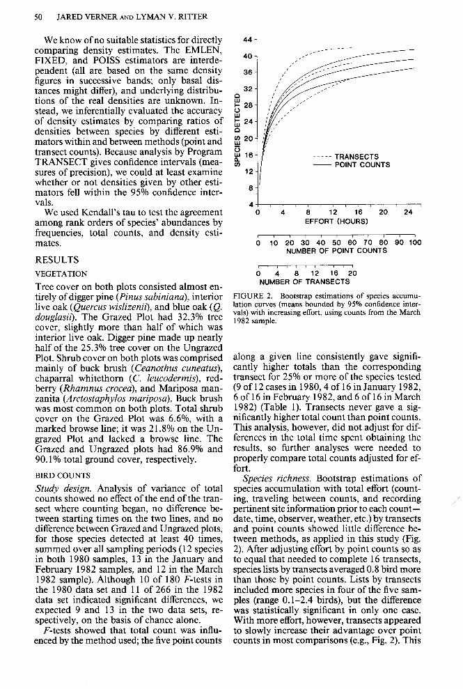
----- TRANSECTS - POINT COUNTS

4-1 I I I I I I !, I I I I I 0 4 8 12 16 20 24

EFFORT (HOURS)

, ! I I I I I I I II 0 lo 20 30 40 50 60 70 80 90 100

NUMBER OF POINT COUNTS

I I I I I I I I I I 0 4 8 12 16 20

NUMBER OF TRANSECTS

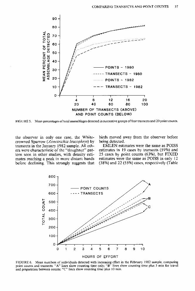
FIGURE 2. Bootstrap estimations of species accumulation curves (means bounded by 95% confidence intervals) with increasing effort, using counts from the March 1982 sample.

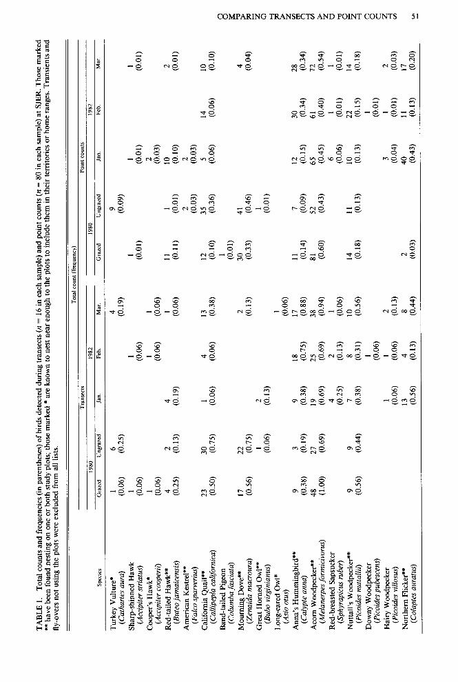
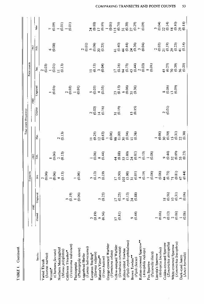
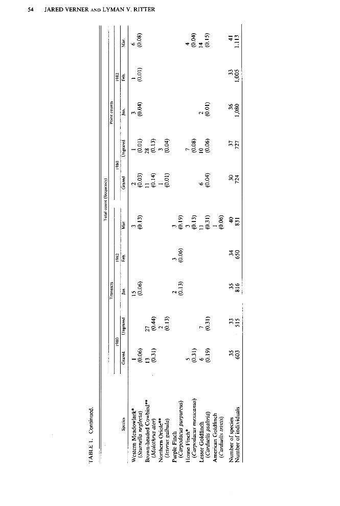
along a given line consistently gave significantly higher totals than the corresponding transect for 25% or more of the species tested (9 of 12 cases in 1980,4 of 16 in January 1982, 6 of 16 in February 1982, and 6 of 16 in March 1982) (Table 1). Transects never gave a significantly higher total count than point counts. This analysis, however, did not adjust for differences in the total time spent obtaining the results, so further analyses were needed to properly compare total counts adjusted for effort.

Species richness. Bootstrap estimations of species accumulation with total effort (counting, traveling between counts, and recording pertinent site information prior to each count - date, time, observer, weather, etc.) by transects and point counts showed little difference between methods, as applied in this study (Fig. 2). After adjusting effort by point counts so as to equal that needed to complete 16 transects, species lists by transects averaged 0.8 bird more than those by point counts. Lists by transects included more species in four of the five samples (range 0.1-2.4 birds), but the difference was statistically significant in only one case. With more effort, however, transects appeared to slowly increase their advantage over point counts in most comparisons (e.g., Fig. 2). This

i

COMPARING TRANSECTS AND POINT COUNTS 5 5

----- TRANSECTS __ POINT COUNTS

4’p 0 4 a 12 16 20 24 28 32

EFFORT (HOURS)

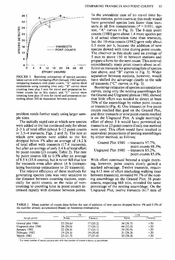
FIGURE 3. Bootstrap estimations of species accumulation curves with increasing effort (January 1982 sample), comparing transects with point counts. “A” curves show estimations using counting time only; “B” curves show counting time plus 5 min for travel and preparation between counts (as in this study), and “C” curves show counting time plus 10 min for travel and preparation (assuming about 300-m separation between points).

problem needs further study using larger sample sizes.

The initially rapid rate at which new species were added to the list continued only for about 2-3 h of total effort (about 8-12 point counts or 2.5-4 transects; Figs. 2 and 3). The rate at which new species were added to the list dropped below 1% after an average of 14.2 h of total effort with transects (17.4 transects), but after an average of only 5.4 h of total effort by point counts (23 counts; Table 2). The rate by point counts fell to 0.5% after an average of 8.5 h (35.8 counts), but it never fell that low for transects even after about 16 h (extrapo- lating bootstrap estimations to 20 transects).

The relative efficiency of these methods for generating species lists was very sensitive to the distance between counting stations, especially for point counts, as the ratio of non- counting to counting time in point counts increased rapidly with distance between points.

In the unrealistic case of no travel time between stations, point counts in this study would have generated species lists faster than transects in all five comparisons (P = 0.03 1, sign test; “A” curves in Fig. 3). The 8-min point counts (1980) gave about 1.4 more species per h of actual observation time than transects, but the 1 0-min counts (1982) gave only about 0.5 more per h, because the addition of new species slowed with time during point counts. The observer in this study used an average of 5 min to move 150 m between stations and prepare a form for the next count. This interval coincidentally made point counts about as efficient as transects for generating lists of species (see above, and “B” curves in Fig. 3). Wider separation between stations, however, would have shifted the advantage clearly to the side of transects (“C” curves in Fig. 3).

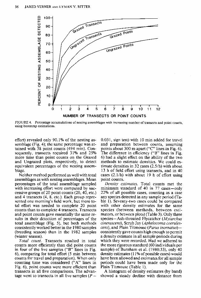
Bootstrap estimates of species accumulation curves, using only the nesting assemblages for the Grazed and Ungrazed plots in 1980, showed that little effort was needed to detect at least 70% of the assemblage by either point counts or transects (Fig. 4). One transect or five point counts reached that goal on the Grazed Plot, and three transects or nine point counts reached it on the Ungrazed Plot. A single morning’s effort of about 5 h would have permitted six transects or 23 point counts if only one method were used. This effort would have resulted in equivalent proportions of nesting assemblages by either method, as follows:

Grazed Plot 1980 -transects 97.7%, point counts 98.3%;

Ungrazed Plot 1980 -transects 85.2%, point counts 8 5.6%.

With effort continued beyond a single morning, however, point counts slowly gained a marked advantage. Twelve transects, requiring 6 13 min of effort (including walking time between transects), revealed 99.7% ofthe nesting assemblage on the Grazed Plot; 38 point counts, requiring 468 min, revealed the same percentage of the nesting assemblage. On the Ungrazed Plot, twelve transects (617 min of

TABLE 2. Mean number of counts done before the rate of addition of new species dropped below 1% and 0.5% of the number already accumulated (based on bootstrap estimations).

I %

Sample period Poillts Transects

Grazed plot 1980 22 (24.6)’ 17 (33.2) Ungrazed plot 1980 28 (29.0) 17 (34.1) January 1982 22 (28.4) 17 (33.1) February 1982 19 (24.3) 19 (30.4) March 1982 23 (31.7) 17 (37.6)

I The mean number of species accumulated wth that number of counts is shown in parentheses.

0.5%

POlntS T’raWXtS

34 (26.7) >20 44 (32.3) >20 35 (30.9) >20 31 (26.3) >20 35 (34.3) >20


FIGURE 4.

E loo- t-

t? go-

k 80-

z I: 70-

’ : 60-

r/l a 50-

4 i= 40-

$ 30-

$ 20-

5

; ‘O-

: 0 1 I 1 1 I I I 1 I I 1 1

0123456789 10 11 12

NUMBER OF TRANSECTS OR POINT COUNTS

Percentage accumulations of nesting assemblages with increasing number of transects and point using bootstrap estimations.

counts,

effort) revealed only 90.1% of the nesting assemblage (Fig. 4); the same percentage was attained with 38 point counts (494 min). Con- sequently, transects required 31% and 25% more time than point counts on the Grazed and Ungrazed plots, respectively, to detect equivalent percentages of the nesting assemblage.

Neither method performed as well with total assemblages as with nesting assemblages. Mean percentages of the total assemblage sampled with increasing effort were computed by successive groups of 20 point counts (20,40, etc.) and 4 transects (4, 8, etc.). Each group repre- sented one morning’s field work, but more total effort was needed to complete 20 point counts than to complete 4 transects. Transects and point counts gave essentially the same results in their detection of percentages of the total assemblage (Fig. 5), but both methods consistently worked better in the 1980 samples (breeding season) than in the 1982 samples (winter season).

Total count. Transects resulted in total counts more efficiently than did point counts in four of the five samples ((‘B” lines in Fig. 6), comparing for total effort (5 min between counts for travel and preparation). When only counting time was considered (“A” lines in Fig. 6) point counts were more efficient than transects in all five comparisons. The advantage went to transects in all five samples (P =

0.031, sign test) with 10 min added for travel and preparation between counts, assuming points about 300 m apart (“C” lines in Fig. 6). The difference in efficiency (“B” lines in Fig. 6) had a slight effect on the ability of the two methods to estimate densities. We could estimate densities in 32 cases (2.5/h) with about 13 h of field effort using transects, and in 40 cases (2.1/h) with about 19 h of effort using point counts.

Density estimates. Total counts met the minimum standard of 40 in 77 cases-only 22% of all possible cases, counting as a case any species detected in any sample period (Ta- ble 1). Seventy-two cases could be compared with other density estimates for the same species (between methods, between estimators, or between plots) (Table 3). Only three species- Ash-throated Flycatcher (Myiarchus cinerascens), Scrub Jay (Aphelocoma coerules- tens), and Plain Titmouse (Parus inornatus)- consistently gave counts high enough to permit a density estimate in all sample periods during which they were recorded. Had we adhered to the more rigorous standard (60 individuals per sample) of Burnham et al. (1980:33), only 40 density estimates (11% of possible cases) would have been allowed and estimates for all sample periods could have been made only for the Plain Titmouse (Table 1).

A histogram of density estimates (by band) showed a steady decline with distance from


80 -

- POINTS 1980 -

----- TRANSECTS 1980 -

.._ P0,NTS ,982 -

--- TRANSECTS - 1982

00 4 8 12 16 20

20 40 60 80 100

NUMBER 0~ TRANSECTS (ABOVE) AND POINT COUNTS (BELOW)

FIGURE 5. Mean percentages of total assemblages detected in successive groups of four transects and 20 point counts.

the observer in only one case, the White- birds moved away from the observer before crowned Sparrow (Zonotrichia leucophrys) by being detected. transects in the January 1982 sample. All oth- EMLEN estimates were the same as POISS ers were characteristic of the “doughnut” pat- estimates in 19 cases by transects (59%) and tern seen in other studies, with density esti- 25 cases by point counts (63%), but FIXED mates reaching a peak in more distant bands estimates were the same as POISS in only 12 before declining. This strongly suggests that (38%) and 22 (55%) cases, respectively (Table

800,

700

600

- POINT COUNTS

---- TRANSECTS

I 1 I 1 I I I 1 1 I 0 1 2 3 4 5 6 7 8 9 10

HOURS OF EFFORT

FIGURE 6. Mean numbers of individuals detected with increasing effort in the February 1982 sample, comparing point counts and transects. “A” lines show counting time only; “B” lines show counting time plus 5 min for travel and preparation between counts; “c” lines show counting time plus 10 min.


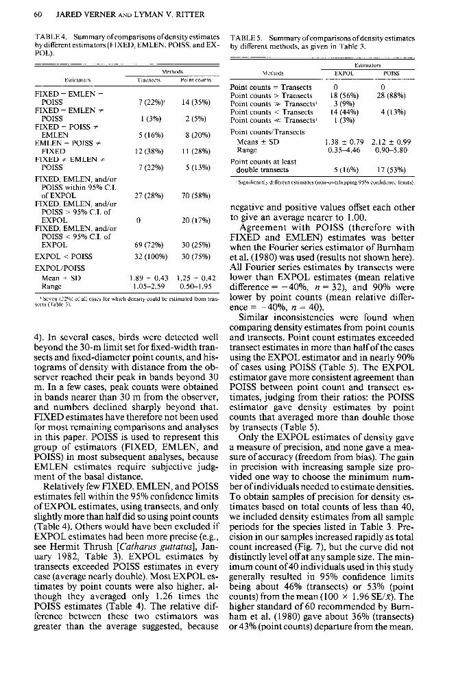
TABLE 4. Summary of comparisons of density estimates by different estimators (FIXED, EMLEN, POISS, and EX- POL).

Methods

Ewmalors T~~llS~CtS Polo1 CO”“,S

FIXED = EMLEN = POISS

FIXED = EMLEN f POISS

FIXED = POISS # EMLEN

EMLEN = POISS + FIXED

FIXED f EMLEN f POISS

FIXED, EMLEN, and/or POISS within 95% C.I. of EXPOL

FIXED, EMLEN, and/or POISS > 95% C.I. of EXPOL

FIXED, EMLEN, and/or POISS < 95% C.I. of EXPOL

EXPOL < POISS

EXPOL/POISS Mean f SD Range

I

I (22%)’ 14 (35%)

1 (3%) 2 (5%)

5 (16%) 8 (20%)

12 (38%) 11 (28%)

7 (22%) 5 (13%)

27 (28%)

0

69 (72%)

32 (100%)

1.89 f 0.43 1.05-2.59

70 (58%)

20 (17%)

30 (25%)

30 (75%)

1.25 k 0.42 0.50-1.95

I Seven (22%) of all cases for which density could be estimated from tran- secls (Table 3).

4). In several cases, birds were detected well beyond the 30-m limit set for fixed-width transects and fixed-diameter point counts, and his- tograms of density with distance from the observer reached their peak in bands beyond 30 m. In a few cases, peak counts were obtained in bands nearer than 30 m from the observer, and numbers declined sharply beyond that. FIXED estimates have therefore not been used for most remaining comparisons and analyses in this paper. POISS is used to represent this group of estimators (FIXED, EMLEN, and POISS) in most subsequent analyses, because EMLEN estimates require subjective judg- ment of the basal distance.

Relatively few FIXED, EMLEN, and POISS estimates fell within the 95% confidence limits of EXPOL estimates, using transects, and only slightly more than half did so using point counts (Table 4). Others would have been excluded if EXPOL estimates had been more precise (e.g., see Hermit Thrush [Cutharus g~ttatu.s], Jan- uary 1982, Table 3). EXPOL estimates by transects exceeded POISS estimates in every case (average nearly double). Most EXPOL estimates by point counts were also higher, although they averaged only 1.26 times the POISS estimates (Table 4). The relative difference between these two estimators was greater than the average suggested, because

TABLE 5. Summary ofcomparisons ofdensity estimates by different methods, as given in Table 3.

Estimators

Methods EXPOL POISS

Point counts = Transects 0 Point counts > Transects 1: (56%) 28 (88%) Point counts z+ Transects 3 (9%) Point counts < Transects 14 (44%) 4 (13%) Point counts K Transects’ 1 (3%)

Point counts/Transects Means f SD Range

Point counts at least

1.38 + 0.79 2.12 f 0.99 0.35-4.46 0.90-5.80

double transects 5 (16%) 17 (53%)

I S~gn~licanll~ dlkcnt estimates (non-overlapping 95% confidence bmlts).

negative and positive values offset each other to give an average nearer to 1.00.

Agreement with POISS (therefore with FIXED and EMLEN) estimates was better when the Fourier series estimator of Bumham et al. (1980) was used (results not shown here). All Fourier series estimates by transects were lower than EXPOL estimates (mean relative difference = -4O%, n = 32), and 90% were lower by point counts (mean relative difference = -4O%, n = 40).

Similar inconsistencies were found when comparing density estimates from point counts and transects. Point count estimates exceeded transect estimates in more than half of the cases using the EXPOL estimator and in nearly 90% of cases using POISS (Table 5). The EXPOL estimator gave more consistent agreement than POISS between point count and transect estimates, judging from their ratios: the POISS estimator gave density estimates by point counts that averaged more than double those by transects (Table 5).

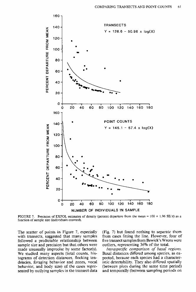
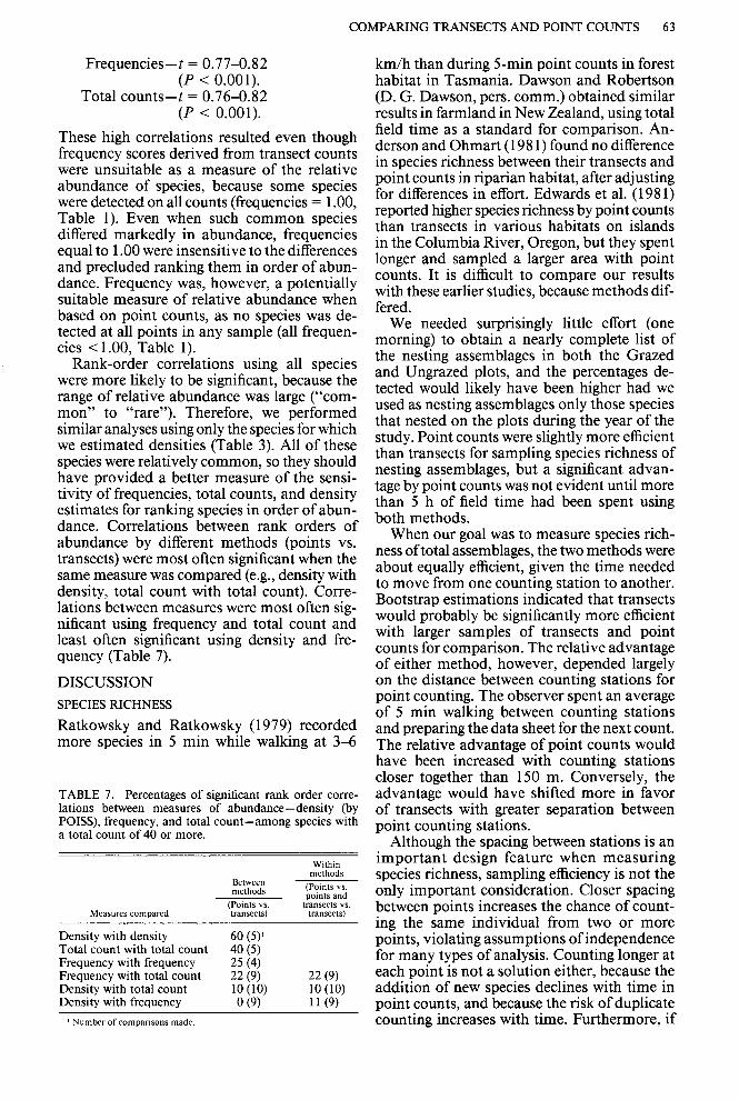
Only the EXPOL estimates of density gave a measure of precision, and none gave a measure of accuracy (freedom from bias). The gain in precision with increasing sample size provided one way to choose the minimum number of individuals needed to estimate densities. To obtain samples of precision for density estimates based on total counts of less than 40, we included density estimates from all sample periods for the species listed in Table 3. Pre- cision in our samples increased rapidly as total count increased (Fig. 7), but the curve did not distinctly level off at any sample size. The minimum count of 40 individuals used in this study generally resulted in 95% confidence limits being about 46% (transects) or 53% (point counts) from the mean (100 x 1.96 SE/,@. The higher standard of 60 recommended by Burn- ham et al. (1980) gave about 36% (transects) or 43% (point counts) departure from the mean.

COMPARING TRANSECTS AND POINT COUNTS 6 1

160

1 TRANSECTS

Y = 126.6 - 50.96 x log(X) z 140-

:

Iz

120- .

. u_ loo- .

ii ”

2 80- .

01 I I I I I I I I I

0 20 40 60 80 100 120 140 160 180

160

140 1 I

. POINT COUNTS

Y = 145.1 - 57.4 x log(X)

80 . .

l .

0, I 1 I 1 I I I I 1

0 20 40 60 80 100 120 140 160 180

NUMBER OF INDIVIDUALS IN SAMPLE

FIGURE 7. Precision of EXPOL estimates of density (percent departure from the mean = 100 x 1.96 SE/K) as a function of sample size (individuals counted).

The scatter of points in Figure 7, especially with transects, suggested that many samples followed a predictable relationship between sample size and precision but that others were made unusually imprecise by some factor(s). We studied many aspects (total counts, his- tograms of detection distances, flocking ten- dencies, foraging behavior and zones, vocal behavior, and body size) of the cases repre- sented by outlying samples in the transect data

(Fig. 7) but found nothing to separate them from cases fitting the line. However, four of five transect samples from Bewick’s Wrens were outliers, representing 36% of the total.

Intraspecific comparison of basal regions. Basal distances differed among species, as expected, because each species had a characteristic detectability. They also differed spatially (between plots during the same time period) and temporally (between sampling periods on


TABLE 6. Ratios of density estimates (by EXPOL), total counts, and frequencies, comparing results from point counts and transects.

Sample

Density estimates Total counts Frequencies

Points TGUW.33 Points Transects Points Transects

Grazed plot 1980 Scrub Jay/Bushtit Ash-throated Flycatcher/Plain Titmouse Scrub Jay/Ash-throated Flycatcher

Ungrazed plot 1980 Plain Titmouse/Bewick’s Wren Scrub Jay/Bewick’s Wren Ash-throated Flycatcher/Plain Titmouse

January 1982 Ruby-crowned Ringlet/Hermit Thrush Golden-crowned Sparrow/Dark-eyed Junco Bewick’s Wren/Dark-eyed Junco

February 1982 Plain Titmouse/Bushtit Ruby-crowned Ringlet/Yellow-rumped Warbler Hermit Thrush/Plain Titmouse

March 1982 Bushtit/Yellow-rumped Warbler Bewick’s Wren/Brown Towhee Ruby-crowned Ringlet/Scrub Jay

0.09 0.22 1.32 0.33 0.37 0.69 2.63 1.30 0.89

1.73 3.14 1.85 1.18 1.56 1.20 0.50 0.39 0.49

0.97 1.41 1.14 4.18 0.86 7.00 1.63 0.68 1.68

0.09 0.42 2.90 1.75 1.65 1.05 3.82 1.51 0.33

1.97 2.04 0.75 0.36 0.44 0.43 3.98 1.39 0.92

1.27 1.15 0.65 0.86 0.95 0.93

1.55 1.27 1.09 1.02 0.53 0.74

0.92 1.43 1.75 5.75 1.49 3.70

2.52 1.90 1.48 1.28 0.58 0.43

1.02 1.05 0.43 0.77 1.43 0.91

1 .oo 1 .oo 1.00

1.00 1.00 0.88

1.09 1.84 2.27

1.33 1.07 0.94

1.00 1.00 1.06

the same plot) within species. Using only species with total counts adequate for density estimation (Table 3), we examined the effects on density estimation when the basal distance from one sample was used with count data for the same species from another sample. Com- parisons between periods on the same plot (1982 samples) were not different from those between plots during the same period (1980 samples), so we combined results. Thirty-four of 93 comparisons (37%) gave the same density estimate with a borrowed basal distance as with the actual basal distance. Twenty-three comparisons gave higher density estimates with the borrowed basal distance, and 36 gave lower estimates, as follows:

Point counts Borrowed estimates higher-z = 118.7%

(n = 11, SD = 14.6). Borrowed estimates lower--X = 66.5%

(n = 20, SD = 19.6).

Transects Borrowed estimates higher--k = 115.7%

(n = 12, SD = 14.7). Borrowed estimates lower--X = 79.1%

(n = 16, SD = 9.6).

Ratios as measures of relative abundance. Ratios of EXPOL estimates of density, total counts, and frequency scores were compared for three randomly selected pairs of species in each sample period (Table 6). Density estimates by point counts and transects showed

the least consistency among ratios. In three cases, one ratio was < 1 and the other was > 1, indicating that the two methods disagreed with respect to which species was more abundant. In seven cases the larger ratio was at least double the smaller. Frequencies were the most consistent. Only one case disagreed as to which species was more abundant, and the larger ratio was at least double the smaller in only two cases. Similar comparisons between density and total count, density and frequency, and total count and frequency, suggest poor agreement between density and the other two measures but rather good agreement between total count and frequency.

Rank orders as measures of relative abundance. Total counts, frequencies, and density estimates are often used to indicate relative abundances of species. Frequencies and total counts (Table 1) performed similarly in ranking species in order of abundance when all species detected in each sample were included, as seen in the range of correlations (Kendall’s tau):

Frequencies correlated with total counts (range among five samples)

Point counts-t = 0.95-0.98 (P < 0.001).

Transects-t = 0.92-0.96 (P < 0.001).

Point counts correlated with transects (range among five samples)


Frequencies--t = 0.77-0.82 (P < 0.001).

Total counts--t = 0.76-0.82 (P < 0.001).

These high correlations resulted even though frequency scores derived from transect counts were unsuitable as a measure of the relative abundance of species, because some species were detected on all counts (frequencies = 1 .OO, Table 1). Even when such common species differed markedly in abundance, frequencies equal to 1 .OO were insensitive to the differences and precluded ranking them in order of abundance. Frequency was, however, a potentially suitable measure of relative abundance when based on point counts, as no species was detected at all points in any sample (all frequencies < 1.00, Table 1).

Rank-order correlations using all species were more likely to be significant, because the range of relative abundance was large (“common” to “rare”). Therefore, we performed similar analyses using only the species for which we estimated densities (Table 3). All of these species were relatively common, so they should have provided a better measure of the sensi- tivity of frequencies, total counts, and density estimates for ranking species in order of abundance. Correlations between rank orders of abundance by different methods (points vs. transects) were most often significant when the same measure was compared (e.g., density with density, total count with total count). Corre- lations between measures were most often significant using frequency and total count and least often significant using density and frequency (Table 7).

DISCUSSION

SPECIES RICHNESS

Ratkowsky and Ratkowsky (1979) recorded more species in 5 min while walking at 3-6

TABLE 7. Percentages of significant rank order correlations between measures of abundance-density (by POISS), frequency, and total count-among species with a total count of 40 or more.

Measures compared

BetWESl methods

(Pomts vs. transects)

Within methods

(Points vs. points and

transects vs. transects)

Density with density 60 (5)’ Total count with total count 40 (5) Frequency with frequency 25 (4) Frequency with total count Density with total count Density with frequency

’ Number of comparisons made.

22 (9j 22 (9) 10 (10) 10 (10) 0 (9) 11 (9)

km/h than during 5-min point counts in forest habitat in Tasmania. Dawson and Robertson (D. G. Dawson, pers. comm.) obtained similar results in farmland in New Zealand, using total field time as a standard for comparison. An- derson and Ohmart (198 1) found no difference in species richness between their transects and point counts in riparian habitat, after adjusting for differences in effort. Edwards et al. (198 1) reported higher species richness by point counts than transects in various habitats on islands in the Columbia River, Oregon, but they spent longer and sampled a larger area with point counts. It is difficult to compare our results with these earlier studies, because methods differed.

We needed surprisingly little effort (one morning) to obtain a nearly complete list of the nesting assemblages in both the Grazed and Ungrazed plots, and the percentages detected would likely have been higher had we used as nesting assemblages only those species that nested on the plots during the year of the study. Point counts were slightly more efficient than transects for sampling species richness of nesting assemblages, but a significant advantage by point counts was not evident until more than 5 h of field time had been spent using both methods.

When our goal was to measure species richness of total assemblages, the two methods were about equally efficient, given the time needed to move from one counting station to another. Bootstrap estimations indicated that transects would probably be significantly more efficient with larger samples of transects and point counts for comparison. The relative advantage of either method, however, depended largely on the distance between counting stations for point counting. The observer spent an average of 5 min walking between counting stations and preparing the data sheet for the next count. The relative advantage of point counts would have been increased with counting stations closer together than 150 m. Conversely, the advantage would have shifted more in favor of transects with greater separation between point counting stations.

Although the spacing between stations is an important design feature when measuring species richness, sampling efficiency is not the only important consideration. Closer spacing between points increases the chance of counting the same individual from two or more points, violating assumptions of independence for many types of analysis. Counting longer at each point is not a solution either, because the addition of new species declines with time in point counts, and because the risk of duplicate counting increases with time. Furthermore, if


point counts are used to estimate density, longer counts are more biased by movement of birds (Scott and Ramsey 198 1, Granholm 1983).

In addition to having efficiency potentially equal to or greater than transects for measuring species richness, point counts offer several other advantages: (1) duration of the counting period can be absolutely controlled, unlike the case with transects; (2) the observer’s attention can be given wholly to the task- transects require some attention to the path being walked; (3) point counts can be set in smaller patches of relatively homogeneous habitat; and, (4) more point counts can be completed per unit of time, increasing sample size and permitting the sampling of a greater variety of sites.

We know of no objective criteria for deter- mining how long to continue sampling in studies seeking to measure the total species richness of an area. We suggest using the rate at which species are added to the list. For example, sampling by transects might be adequate when the rate at which new species are added to the list drops below 1% (about 14 h of field time in this study). An equivalent effort would give about 76 counts of 6-min duration, spaced about 150 m apart. This is probably a better criterion than seeking a fixed proportion of the avifaunal assemblage, because it requires no prior knowledge of that assemblage. We suggest the rate criterion only to stimulate interest in this subject so that more appropriate general guidelines might be found.

TOTAL COUNT

Dawson and Bull (1975) found no difference in efficiency between transects and point counts as methods for accumulating total counts. Svensson (1980) and Anderson and Ohmart (1981) however, found transects to be more efficient than point counts, as we found. De- pending upon the distance between points and duration of counts, point counts could perform as well as transects. We suspect that counts of 6 min, at points about 100 m apart, would make point counts as efficient as transects for accumulating total counts on our plots. How- ever, the extent to which this spacing would violate assumptions of independence between points is unknown.

RANKING SPECIES IN ORDER OF ABUNDANCE

Frequencies. Frequency is an attractive measure of relative abundance because it is available solely from lists of species. In spite of the high correlations in rank orders of abundance between frequency scores and total counts, however, we consider frequency to be a poor

measure of relative abundance. We recommend that it be used only with due caution for its limitations, as follows: (1) Frequencies are useful measures of relative abundance only when they are less than 1 (D. G. Dawson [pers. comm.] believes they are most useful when less than 0.8). Common species are often recorded on all transects of substantial length or point counts of long duration. Consequently, use of frequency as a measure of abundance neces- sarily determines some aspects of study design. (2) Frequencies cannot, after the fact, be adjusted for differences in sampling time or sampling area between studies. The only way to standardize studies to compare frequencies between them is to use precisely the same sampling procedures in all. (3) Frequencies are sensitive to the number of counts done. The number of frequency intervals possible is equal to the number of counts. Ties between species prevent ranking them in order of abundance by frequency, and the number of ties increases as the number of counts declines. (4) Fre- quencies are inappropriate for comparing flocking species with solitary species. The for- mer may outnumber the latter by orders of magnitude but they could have lower frequency scores.

Total counts. Total counts are preferable to frequencies as measures of relative abundance because: (1) rank orders of species abundance by these two measures were often correlated; (2) total counts are nearly as economical to obtain as species lists; (3) they are subject to less bias than frequency when comparing flocking with solitary species (although one is more likely to detect a flock); and, (4) as with frequencies, total counts are sensitive to effort-count duration, transect length, or number of counts. Unlike frequencies, however, total counts can be standardized to area sampled or counting time, after the fact, for comparisons between studies using different de- signs.

Density estimates. We agree with Ramsey and Scott (1979) and Burnham et al. (1980, 198 1) that density estimates are better than total counts as indices of relative abundance. This is because using separate basal regions for each species apparently does make some ad- justment for differences in detectability (see results of Laake 1978, reported in Burnham et al. 1980; also see Skirvin 198 1). Density estimates in our study were sometimes correlated with total counts and frequencies when ranking species in order of abundance, and they showed the best agreement when comparing point counts with transects. They offer the same advantages over frequencies as do total counts. Use of density estimates to index


the abundance of species, however, has a lim- itation not commonly overcome, or even ac- knowledged, in studies of the abundance of birds. Sample sizes much larger than those attained in most studies are required to estimate densities of most species by line transects or point counts with variable limits. For example, we were able to estimate densities in only 32 cases (18% of all possible cases) using transects and in 40 cases (23%) using point counts. We could have estimated densities in about 50% of all cases with about a five-fold increase in field time. About 520 h (104 person-days of sampling at 5 h/day) of transect effort or 760 h (152 person-days of sampling) of point- counting effort would have been needed to estimate densities of all species detected.

In cases with inadequate counts some observers have estimated density by borrowing the basal distance from another species with similar detectability (e.g., Emlen 1971, 1977; Reynolds et al. 1980). We strongly recommend against this procedure, however, because it assumes that the researcher knows the detecta- bilities of all species. Using only cases in which the total count was at least 40, we found that one takes a risk even when applying basal distances from the same species obtained at different times on the same plot or at the same time on different plots. We have a dilemma: if one uses density estimates, only Herculean efforts will allow indexing of the abundance of most or all species detected; unfortunately, both time and cost constraints normally preclude this. If one uses total counts, the indexing of relative abundance will likely be less accurate than with density estimates. Finally, indices using total counts should not be compared with those using density estimates.

ESTIMATING DENSITIES

Ratios of species’ densities. If different methods for estimating density were accurate, ratios of species’ densities should be the same by all methods. Comparisons of such ratios between EXPOL and POISS estimates of density, using results from both point counts and transects, clearly failed to meet this criterion (Tables 5, 6). Moreover, the ratios determined from point counts deviated in both directions from 1 .OO, indicating that, relative to POISS, EXPOL overestimated densities of some species and underestimated those of others. These results mean either (1) that only one method (POISS or EXPOL) delivered accurate estimates of density and the other method both over- and underestimated densities, depending on the species, or (2) that neither method delivered accurate estimates of density, at least for some species. We could not distinguish between these

alternatives from our analysis ofratios, but we believe that alternative #2 is correct, because of the many sources of uncontrolled and un- controllable bias that influence counts of birds (Vemer 1984).

Comparisons of estimators. General agreement among the density estimates given by EMLEN, FIXED, and POISS is not evidence that they are accurate estimators. They are similar analytical procedures, using the same data sets and the same grouping intervals. The only variable among them is basal distance. Cases with the same basal distance will give identical density estimates. The generally poorer agreement between FIXED and the other two estimators resulted from the fact that some species were readily detectable at greater distances than others.

The generally poor agreement between EX- POL estimates and those of POISS, EMLEN, and FIXED, allows no firm conclusion about the accuracy of any of these estimators. At best, one is more accurate than another. EX- POL may be the best among them, however, because it is less negatively biased by movement of animals than all other estimators tested by Bumham et al. (1980). Indirect evidence from our study also suggests that the EXPOL estimator may be more accurate than the others. Transects using the EMLEN estimator consistently give lower density estimates than spot mapping (Emlen 197 1, 1977; Franzreb 1976, 198 l), which many observers assume to be reasonably accurate. Because our density estimates by EXPOL were consistently higher than those by EMLEN (and all other estimators as well), they may be more comparable to estimates using spot mapping. In any case, EXPOL merits further study as an estimator of bird densities to use with transects and point counts.

Comparisons of point-count and transect methods. The poor agreement between methods using the POISS estimator is especially noteworthy, as the average point-count estimate by POISS was more than double that by transects. Although the EXPOL estimates showed better agreement, the two methods by EXPOL failed to show a consistent bias- some point-count estimates were higher and some were lower than the corresponding transect estimates. In some cases, the discrepancy was clearly unacceptable (e.g., point count estimates from 35% to 446% of the corresponding transect estimate, using EXPOL, and from 90% to 580% using POISS, Table 5).

Transects gave more consistent results than point counts (e.g., better precision, Fig. 7; all EXPOL estimates higher than POISS estimates, Table 4; and better agreement between


basal distances of the same species between spatially and temporally different samples). This probably resulted from differential vio- lation of at least one major assumption of the models, namely, that all distances from the transect line or the counting point to the bird were correctly estimated. The effect of any systematic bias in distance estimation was am- plified in point counts by comparison with transects, because area sampled increased linearly with distance in transects but with distance squared in point counts.

These data may indicate that densities of some species are accurately estimated by one or both methods, using one or both estimators, but we cannot identify any species for which this may be true. It is also clear that neither method nor estimator should be assumed to give accurate interspecific comparisons of density estimates without considerably more study, including comparisons with populations whose densities are better known, as by intensive study of banded birds.

Precision of estimates. The large 95% confidence limits about the mean of EXPOL estimates generally indicate that the density estimate of a more abundant species must be at least twice that of a less abundant one before the difference would be significant at an alpha level of 0.05. The same would apply to intraspecific comparisons, either spatially or temporally. The situation is improved with larger samples, requiring greater effort (see “ranking species in order of abundance”).

Meeting assumptions of models. All estimators assume that movements by birds in response to the observer do not affect results (e.g., Ramsey and Scott 1978, Burnham et al. 1980). The “doughnuts” seen in most histo- grams of detections with distance from the observer could have resulted from (1) movement of birds away from the observer, (2) attraction ofbirds toward the observer from more distant points, (3) “freezing” by birds near the observer to avoid detection, or (4) some com- bination of these events. Movement by birds was probably most responsible for the reduced numbers of birds detected near observers. Granholm (1983) estimated that movement by birds resulted in as much as a 56% over- estimate of density on plots with fixed radii of 30 m. Burnham et al. (1980:2 1) concluded that, “If the subject of the study is a highly mobile animal (such as a passerine bird), serious problems due to movement can arise, often to the extent of rendering line transect sampling use- less for such species.”

The EXPOL estimator assumes that all individuals on the transect line or counting point are detected, and the FIXED, EMLEN, and

POISS estimators assume that all individuals out to the basal distance are detected. Jolly (198 1:216) stated that, “The major cause of underestimation . . . is likely to be that birds are being missed ‘close’ to the observer.” By definition, we cannot evaluate our data quan- titatively with respect to this assumption. We have occasionally detected birds that appeared to hide from us near transect lines, so some near birds probably avoided detection and others were probably missed because they were quiet and obscured by dense vegetation within 30 m of the observer.

Undoubtedly some birds were counted more than once along a given transect or from the same counting point, violating an assumption of all estimators. These could have been bal- anced in some fashion by birds missed, but the equivalency of these compensating biases was unknown and could not be assumed to elim- inate these problems. Accurate measurement of distance is another assumption common to all estimators, being less critical for FIXED estimates because only one distance must be learned. We believe our results did not seri- ously violate this assumption, because distance estimation was facilitated by the stakes at intersections of the grid on both plots, and the observer was thoroughly familiar with the plots from extensive field work on them since 1977. But any systematic errors would have influenced estimates from point counts more than those from transects, as discussed pre- viously.

CONCLUSIONS

The regularity and magnitude of inconsistencies found in this study in the ratios of species’ densities, comparisons of estimators, and comparisons of methods present a strong chal- lenge to any assumption that these methods deliver reasonably accurate estimates of the densities of birds. Other evidence suggests that several key assumptions of the models were violated by our data. This is not surprising, given the many biases known to influence counts of birds (Verner 198 1, 1984; Dawson and Verner, unpubl.). Many papers in Ralph and Scott (198 1) address various sources of bias. Taken together, these lines of evidence leave us unconvinced that either transects or point counts estimate densities of most or all species accurately enough to satisfy objectives of most studies.

More research is needed to assess the accuracy of these methods for estimating densities of birds. Meanwhile, if our results are typical, transects and point counts should not be used when accurate estimates of densities are needed, as in studies of trophic dynamics.


Similarly, calculation of species diversity indices should not rely on density estimates from these methods, because they are not likely to give comparable estimates of all species (i.e., on a ratio scale). Whether or not the method can rank species in the correct order of abundance with reasonable accuracy still needs ver- ification. We advise caution even when using the methods to make intraspecific comparisons between habitats or seasons, because detectability probably differs with differences in vegetation structure, and it certainly differs seasonally. We question the wisdom of using these methods to compare abundances among different species, either in the same or in different habitats or seasons. Differences in detectability between species are well-known.

Transects and point counts surely have a place in assessing intraspecific trends in population size in the same locality, if all samples are taken during the same phenological period. When used for other purposes, their results should be interpreted with caution. The great- est danger in using these methods to answer questions beyond their capability lies in the fact that results, once published, tend to attain a measure of credibility, especially after they have been cited by others.

ACKNOWLEDGMENTS

J. A. Baldwin, M. R. Bryan, C. J. Evans, L. Maxwell, and D. A. Sharpnack provided consultation and assistance with the study design and data analysis. D. G. Dawson, D. F. DeSante, M. L. Morrison, B. R. Noon, C. J. Ralph, F. L. Ramsey, and R. C. Szaro offered many valuable sugges- tions for improving the manuscript. We express our sin- cere appreciation to all.

LITERATURE CITED ANDERSON, B. W., AND R. D. OHMART. 198 1. Compar-

isons of avian census results using variable distance transect and variable circular plot techniques, p. 186- 192. In C. J. Ralph and J. M. Scott [eds.], Estimating numbers of terrestrial birds. Stud. Avian Biol. 6.

BURNHAM, K. P., D. R. ANDERSON, AND J. L. LAAKE. 1980. Estimation of density from line transect sampling of biological populations. Wildl. Monogr. 7 1: l-202.

BURNHAM, K. P.. D. R. ANDERSON, AND J. L. LAAKE. 198 1. Line transect estimation of bird population density usine a Fourier series. D. 466-482. In C. J. Raloh and J. c Scott [eds.], E&mating numbers of teGestria1 birds. Stud. Avian Biol. 6.

DAWSON, D. G., AND P. C. BULL. 1975. Counting birds in New Zealand forests. Notomis 11: 101-109.

EDWARDS, D. K., G. L. DORSEY, AND J. A. CRAWFORD. 198 1. A comparison of three avian census methods, p. 170-176. In C. J. Ralph and J. M. Scott [eds.], Estimating numbers of terrestrial birds. Stud. Avian Biol. 6.

EFRON, B., AND G. GONG. 1983. A leisurely look at the bootstrap, the jackknife, and cross-validation. Am. Stat. 37~36-48.

EMLEN, J. T. 197 1. Population densities of birds derived from transect counts. Auk 88:323-342.

EMLEN, J. T. 1977. Estimating breeding season bird densities from transect counts. Auk 94:455-468.

FRANZREB, K. E. 1976. Comparison of variable strip transect and spot-map methods for censusing avian populations in a mixed-coniferous forest. Condor 78: 260-262.

FRANZREB, K. E. 198 1. A comparative analysis of ter- ritorial mapping and variable-strip transect censusing methods, p. 164-169. In C. J. Ralph and J. M. Scott [eds.], Estimating numbers of terrestrial birds. Stud. in Avian Biol. 6.

GRANHOLM, S. L. 1983. Bias in density estimates due to movement of birds. Condor 85:243-248.

JARVINEN, O., AND R. A. V;~IS;~NEN. 1975. Estimating relative densities of breeding birds by the line transect method. Oikos 26:3 16-322.

JOLLY, G. M. 198 1. Summarizing remarks: comparison of methods. D. 2 15-2 16. In C. J. Raluh and J. M. Scott [eds.],’ Estimating numbers of terrestrial birds. Stud. in Avian Biol. 6.

LAAICE, J. L. 1978. Line transect estimators robust to animal movement. M.Sc. thesis, Utah State Univ., Logan.

LAAKE, J. L., K. P. BURNHAM, AND D. R. ANDERSON. 1979. User’s manual for program TRANSECT. Utah State Univ. Press, Logan.

NEAL, D. L. 1980. Blue oak-digger pine, p. 126-127. In F. H. Eyre [ed.], Forest cover types of the United States and Canada. Society of American Foresters, Washington, DC.

RALPH, C. J., AND J. M. SCOTT [EDS.]. 1981. Estimating numbers of terrestrial birds. Stud. Avian Biol. 6.

RAMSEY, F. L., AND J. M. SCOTT. 1978. Use of circular plot surveys in estimating the density of a population with Poisson scattering. Tech. Rep. 60, Dept. of Sta- tistics, Oregon State Univ., Corvallis.

RAMSEY, F. L., AND J. M. SCOTT. 1979. Estimating population densities from variable circular plot surveys, p. 155-181. In R. M. Cormack, G. P. Patil, and D. S. Robson [eds.], Sampling biological populations. Stat. Ecol. Ser., Vol. 5. International Co-operative Pub- lishing House, Fairland, MD.

RAMSEY, F. L., AND J. M. SCOTT. 198 1. Analysis of bird survey data using a modification of Emlen’s method, p. 483-487. In C. J. Ralph and J. M. Scott [eds.], Estimating numbers of terrestrial birds. Stud. Avian Biol. 6.

RATKOWSKY, A. V., AND D. A. RATKOWSKY. 1979. A survey of the birds of the Mt. Wellington Range, Tas- mania, during the non-breeding months. Emu 78:223- 226.

REYNOLDS, R. T., J. M. SCOTT, AND R. A. NUSSBAUM. 1980. A variable circular-plot method for estimating bird numbers. Condor 82:309-313.

ROBINETTE, W. L., C. M. LOVELESS, AND D. A. JONES. 1974. Field tests of strip census methods. J. Wildl. Manage. 38:81-96.

SCOTT, J. M., AND F. L. RAMSEY. 198 1. Length of count period as a possible source of bias in estimating bird numbers, p. 409-413. In C. J. Ralph and J. M. Scott [eds.], Estimating numbers of terrestrial birds. Stud. Avian Biol. 6.

SKIRVIN. A. A. 198 1. Effect of time of day and time of season on the number of observationi and density estimates ofbreedina birds. D. 272-274. In C. J. Raloh and J. M. Scott [eds.], Estimating numbers of terrestrial birds. Stud. Avian Biol. 6.

SVENSSON, S. 1980. Comparison of recent bird census methods, p. 13-22. In H. Oelke [ed.], Bird census work and nature conservation. Proceedings of the VI International Conference on Bird Census Work. Univ. Gt)ttingen, West Germany.

TILGHMAN, N. G., AND D. H. RUSCH. 198 1. Comparison of line-transect methods for estimating breeding bird


densities in deciduous woodlots, p. 202-208. In C. J. 247-302. In R. F. Johnston, [ed.], Current omithol- Ralph and J. M. Scott [eds.], Estimating numbers of ogy. Vol. 2. Plenum Publishing, New York. terrestrial birds. Stud. Avian Biol. 6.

VERNER, J. 198 1. Introductory remarks: sampling de- Pacific Southwest Forest and Range Experiment Station, sign, p. 391. In C. J. Ralph and J. M. Scott [eds.], Forest Service, United States Department of Agriculture, Estimating numbers of terrestrial birds. Stud. Avian 2081 East Sierra Avenue, Fresno, California 93710. Re- Biol. 6. ceived 10 November 1983. Final acceptance 20 October

VERNER, J. 1984. Assessment of counting techniques, p. 1984.

The Condor 87:68 0 The Cooper Ornithological Society 1985

RECENT PUBLICATIONS

Intensive regulation of duck hunting in North America: its purpose and achievements.-Hugh Boyd. 1983. Occa- sional Paper No. 50. 24 p. Paper cover. Catalogue No. CW 69-l/50 E. Human dimensions of migratory game- bird hunting in Canada.-Fern L. Filion and Shane A. D. Parker. 1984. Occasional Paper No. 5 1. 34 p. Paper cover. Cataloaue No. CW 69-1151 E. Components of hunting mortal& in ducks.-G. S. Hochbaum and C. J. Wac ters. 1984. Occasional Pauer No. 52. 29 D. Paoer cover. Catalogue No. CW 69-1152 E. All published by the Ca- nadian Wildlife Service. No prices given. Source: Minister of Supply and Services, Ottawa, Canada. These three papers deal with related aspects of a special case ofpredation, the hunting of game-birds by humans. Boyd examines the impact of regulations on the amount of hunting, the reported kill, and population size for ducks in the U.S. and Canada. Filion and Parker discuss the results of a socio- logical survey on the attitudes, hunting practices, expen- ditures, and sources of satisfaction or dissatisfaction of hunters. Hochbaum and Walters evaluate waterfowl hunting and kill on the Delta Marsh, Manitoba, using a mod- ified predator-prey model, by monitoring the numbers and behavior of ducks and hunters. All three are well orga- nized, thought-provoking, and widely applicable. They are each furnished with graphs and lists of references.

Marine birds: their feeding ecology and commercial fisheries relationshios.-Edited bv David N. Nettleship, Gerald A. Sange;, and Paul F. Springer. 1984. A special publication compiled by the Canadian Wildlife Service for the Pacific Seabird Group. 220 D. Paper cover. No mice given. Source: as above. Catalogue No. CW 66-65/1984. This volume presents revised and refereed versions of many of the papers that were given as a special symposium of the 1982 meeting of the Pacific Seabird Group. The first of three sessions “comprises six papers which discuss aspects of the winter or summer feeding ecology of six waterfowl species inhabiting coastal waters of Alaska and British Columbia.” The seven papers of the second session concern the feeding ecology of pelagic marine birds, either at sea or at breeding colonies. The last ten papers “attempt to show the inter-relationships among [seabird] species and the serious effects that commercial fisheries can have on seabird populations and communities by competing directly for food and by accidental drowning of birds in fish nets.” Most of the papers deal with birds of the north- east Pacific or north Atlantic oceans. They neatly report new findings and indicate directions for future research but do not give any of the discussions among the symposium participants. The volume itself has been attrac- tively designed in the accustomed style of CWS publications. The papers are individually furnished with illustrations and lists of references.

Waterfowl on a Pacific estuary.-Barry Leach. 1982. Brit- ish Columbia Provincial Museum Special Publication No. 5. 210 p. Paper cover. No price given. Source: Publica- tions. British Columbia Provincial Museum, 675 Belle- ville Street, Victoria, British Columbia V8V 124, Canada. Author and artist Barry Leach presents the waterfowl of the lower Fraser River as the central theme of his highly readable natural-and sometimes personal-history of British Columbia’s most important river. His pen-and-ink drawings of waterfowl, after the style of H. Albert Hoch- baum, contribute greatly to this environmental history book. Bibliography. Index. Folded map. -J. Tate.

The Trumpeter Swan.-Winston E. Banko. 1980. Uni- versity ofNebraska Press, Lincoln. 2 14 p. $5.95. A reprint of the book first nublished bv the U.S. Fish and Wildlife Service in 1960. *Keeping this work in print is a valuable service, yet it is too bad that the opportunity was missed to add new information on the status and biology of the Trumpeter Swan. - J. Tate.

Coastal waders and wildfowl in winter.-P. R. Evans, J. D. Goss-Custard and W. G. Hale, eds. 1984. Cambridge University Press, Cambridge. 331 p. $54.50. This is a gathering of papers on food selection and habitat usage by migrant and wintering shorebirds and waterfowl in tidal marshes and intertidal zones of the Palearctic-African coastal area. The first six papers discuss the influence of food resources on the level of usage of feeding areas. The next five papers examine mechanisms of usage of feeding areas with an emphasis on social behavioral controls. A final group ofeight papers deals with specific locations and their significance to the shorebird populations. The volume offers some additional data on food and habitat usage by waterfowl and much new information on shorebirds and their prey. References following each paper. Index. - J. Tate.

A field guide to the warblers of Britain and Europe.- AlickMoore. 1983. OxfordUniversity Press. 145 p. $18.95. Fifty-three species of Old World warblers (Sylviinae, Mus- cicanidael as delineated bv Voous (Ibis 119: 242-2451 are discussed’in a field guide-like format. The author warns against hasty identifications, and in favor of paying great attention to details of behavior, plumage, and song. He describes plumages in detail while avoiding the ratios and measurements used for identification of museum skins. The color plates by Bryon Wright carefully show color and subtle shading ofplumage and soft parts. Song descriptions are uninspired and often confusing. The binding is that of a shelf book rather than a field guide. Detailed range maps. List of references. Index.- J. Tate.

Documents

A Comparison of Transects and Point Counts in Oak-pine ... · A COMPARISON OF TRANSECTS AND POINT COUNTS IN OAK-PINE WOODLANDS OF CALIFORNIA JARED VERNER AND LYMAN V. RITTER ABSTRACT.-Transects