A Comparison of Rendering Techniques for 3D Line Sets with

1077-2626 (c) 2019 IEEE. Personal use is permitted, but republication/redistribution requires IEEE permission. See http://www.ieee.org/publications_standards/publications/rights/index.html for more information.

This article has been accepted for publication in a future issue of this journal, but has not been fully edited. Content may change prior to final publication. Citation information: DOI 10.1109/TVCG.2020.2975795, IEEETransactions on Visualization and Computer Graphics

1

A Comparison of Rendering Techniquesfor 3D Line Sets with Transparency

Michael Kern, Christoph Neuhauser, Torben Maack, Mengjiao Han, Will Usher, Rudiger Westermann

Abstract—This paper presents a comprehensive study of rendering techniques for 3D line sets with transparency. The rendering oftransparent lines is widely used for visualizing trajectories of tracer particles in flow fields. Transparency is then used to fade out linesdeemed unimportant, based on, for instance, geometric properties or attributes defined along with them. Accurate blending oftransparent lines requires rendering the lines in back-to-front or front-to-back order, yet enforcing this order for space-filling 3D line setswith extremely high-depth complexity becomes challenging. In this paper, we study CPU and GPU rendering techniques for transparent3D line sets. We compare accurate and approximate techniques using optimized implementations and several benchmark data sets.We discuss the effects of data size and transparency on quality, performance, and memory consumption. Based on our study, wepropose two improvements to per-pixel fragment lists and multi-layer alpha blending. The first improves the rendering speed via animproved GPU sorting operation, and the second improves rendering quality via transparency-based bucketing.

Index Terms—Scientific visualization, line rendering, order-independent transparency.

F

1 INTRODUCTION

In many visualization tasks, the need to efficiently dis-play sets of 3D lines is paramount. Applications rangefrom the visualization of pathways of particle tracers inflow fields or over moving vehicles for smart transportationand urban planning, to exploring neural connections inthe brain or relations encoded in large graphs and net-work structures. Prior work such as [3], [12], [19], [27]has shown that transparency, when used carefully to avoidoverblurring, can be used effectively to relieve occlusionsand to accent important structures while maintaining lessimportant context information. It is particularly useful forexploratory visualization tasks, where users interactivelyselect the strength of transparency and the mapping of datavalues to transparency.

Rendering transparency, however, introduces a perfor-mance penalty. When using transparency, the per-pixel colorand opacity contributions need to be blended in correctvisibility order, i.e., by using α-blending (where α representsa point’s opacity) in either front-to-back or back-to-frontorder. Rendering techniques can be distinguished as towhether they compute the visibility order exactly or approx-imately, and how this order is established. Especially for linesets, which have a significantly higher depth complexitythan surface or point models, maintaining the visibilityorder during rendering can become a severe performancebottleneck.

In this study, we evaluate exact and approximate object-and image-order transparency rendering techniques, with

• M. Kern, C. Neuhauser, T. Maack, and R. Westermann are with theComputer Graphics & Visualization Group, Technische UniversitatMunchen, Garching, GermanyE-mail: {michi.kern, christoph.neuhauser, westermann}@tum.de,[email protected]

• M. Han and W. Usher are with the Scientific Computing and ImagingInstitute, University of Utah, U.S.E-mail: {mengjiao, will}@sci.utah.edu

intending to analyze the performance of such techniqueswhen used to render line sets with an extremely highdepth complexity. Our evaluation includes an in-depth eval-uation of model-specific acceleration schemes. We furtherdemonstrate the use of approximate transparency renderingtechniques for surface and point models with high depthcomplexity, though refrain from a detailed performanceevaluation on these cases. The latter would require consider-ing specific acceleration structures for such surface or pointmodels, which is beyond the scope of a single paper.

Object-order techniques make use of GPU rasterization.We consider Depth Peeling (DP) [10] and Per-Pixel LinkedLists (LL) [43], both of which can render transparency ac-curately at the cost of computing or memory. Other object-order techniques use (stochastic) transmittance approxima-tions, where transmittance refers to the multiplicative ac-cumulation of per-fragment transparencies. Of the manydifferent variants of approximate techniques, we selectedMulti-Layer Alpha Blending (MLAB) [32] and the most re-cent Moment-Based Blending Technique (MBOIT) [25] (seeFig. 1 for example images). Both approximate techniquesuse only small and constant additional buffer resources.

We also evaluate four image-order techniques based onray-tracing. We consider the Generalized Tubes method [13]as well as Embree’s built-in Bezier curve primitives [40]implemented in Intel’s OSPRay CPU ray-tracing framework(OSP) [38], a GPU ray-tracer using NVIDIA’s RTX ray-tracing interface [26] through the Vulkan API (RTX), andvoxel-based GPU line ray-tracing (VRC) [15]. All techniquesutilize dedicated data structures to facilitate efficient raytraversal as well as empty space skipping and thus provideeffective means to evaluate the capabilities of image-orderline rendering.

OSP, RTX, VRC, DP, and LL, despite their algorithmicdifferences, are all accurate methods and yield the samerendering result. Performance-wise, on the other hand, thesetechniques differ substantially, and for large data sets some

Authorized licensed use limited to: The University of Utah. Downloaded on February 26,2020 at 04:26:16 UTC from IEEE Xplore. Restrictions apply.



2

(a) (b)

(c)

(a) PSNR = 33.41, SSIM = 0.907 (b) PSNR = 31.98, SSIM = 0.901

(d)

(c) PSNR = 34.42, SSIM = 0.913 (d) PSNR = 31.10, SSIM = 0.842

Fig. 1: Strengths and weaknesses of transparent line rendering techniques. For each pair, the left image shows the groundtruth (GT). Right images show (a) approximate blending using MLABDB, (b) opacity over-estimation of MBOIT, (c) reverseblending order of MLABDB, (d) blur effect of MBOIT. Speed-ups to GT rendering technique: (a) 7, (b) 2, (c) 3.5, (d) 4.5.

of them even turn out to be impractical. The main goal of ourevaluation study is to shed light on the differences betweenthese techniques and to provide guidelines for selecting asuitable rendering technique for a given application.

ContributionWe provide a qualitative and quantitative comparison oftechniques for rendering 3D line sets with transparency.For our evaluation, we have systematically selected a setof techniques that we believe are representative for thedifferent principal approaches that are available today. Eventhough our evaluation study has been performed solelyon 3D line sets, the results are also applicable to otherapplication scenarios where transparency is used to revealotherwise hidden structures.

Through our study, users and practitioners can gainan understanding of the principal implications of using acertain technique and become aware of their major strengthsand limitations with respect to quality, memory require-ments, and performance. Since we use a range of differentsized data sets with vastly different internal structures, ourevaluation hints to specific data-dependencies of certainrendering concepts. We tried to individually select a trans-parency setting for each data set that reveals importantfeatures in a meaningful way. Thus, we consider our resultsrepresentative of typical use cases of transparent line ren-dering. For each technique, we also analyze the pre-processthat is required to build the data representations needed forrendering and perform a thorough evaluation of renderingperformance.

Moreover, we have modified LL to improve scalabilitywith the number of fragments, and MLAB to make it lessdependent on the order of fragments per pixel. For LL, wedeveloped GPU-friendly variants of shell-sort and priority-queues through the min-heap data structure, resulting ina performance increase of a factor of 2-3. Our implemen-tation of MLAB uses a discrete set of depth intervals andcan considerably reduce the number of incorrectly mergedfragments.

We have made our implementations publicly avail-able [17], the test environment using NVIDIA’s RTX [20],all data sets [16], and all benchmark results for imagequality and performance evaluation. We have also includedadditional descriptions of how to use the implementationsand apply them to other data sets.

2 RELATED WORK

Prior work [22], [42] has compared some of the many dif-ferent rendering techniques for transparent geometry. Theseevaluations, however, have mainly focused on the use oftechniques for real-time graphics effects in scenes comprisedof a few spatially extended and homogeneous transparentobjects with rather low depth complexity. Thus, the suitabil-ity of techniques for visualization tasks as outlined in ourwork is difficult to infer from available evaluations. To thebest of our knowledge, an evaluation and comparison oftechniques for rendering large 3D line sets, including ray-based approaches and scenes with extremely high depthcomplexity and high-frequency transmittance functions, hasnot been performed.

2.1 Object-order techniques

Several approaches have been proposed to blend the frag-ments falling into the same pixel in correct visibility orderwithout having to resort to an explicit sorting of geometry.Everitt et al. [10] presented depth peeling, which renders foreach pixel in the i-th rendering pass the i-th closest surfacepoint using a second depth buffer test against the valuesfrom the previous pass. In early work by Carpenter [6], theA-buffer was introduced as a data structure that stores theunordered set of fragments falling into each pixel. Thesefragments are then sorted explicitly based on the storeddepth information. Yang et al. [43] used per-pixel linkedlists to store a variable number of fragments per pixel onthe GPU, after which they are sorted to blend the fragmentsin correct order. Contrary to the linked lists, the k-Buffer [4]




3

stores only the k nearest fragments, and merges fragmentsheuristically if more than k fall into the same pixel.

In scenarios where the k-Buffer is not applicable, frag-ments have to be blended heuristically. Adaptive Trans-parency [31] operates on k fragments and aims to storean approximation of the transmittance function per pixel.Alpha blending is then performed in a second pass us-ing this approximation. Maule et al. [21] proposed HybridTransparency, which aggregates fragments using a k-Bufferand merges them heuristically with respect to depth andopacity. Even though this approach is order-independent,it is not able to cope with scenes containing many layers.Multi-Layer Alpha Blending (MLAB) [32] is a single-passtechnique that uses a fixed number of per-pixel transmit-tance layers to approximate the transmittance along a viewray. When all layers are occupied and the current fragmentcreates a new layer, the two most appropriate adjacent layersare merged in turn. Stochastic Transparency [9] uses weightsto blend or discard fragments based on opacity. Weighted-Blended Order-Independent Transparency [23] proposed touse weights based on occlusion and distance to the camerato merge fragments.

Recently, Munstermann et al. [25] introduced Moment-Based Order-Independent Transparency (MBOIT). Rojo etal. [3] demonstrated the embedding of importance-basedtransparency control into MBOIT. MBOIT approximates thetransmittance function pixel-wise by power moments ortrigonometric moments, and applies logarithmic scalingto the absorbance to enforce order-independency and fa-cilitate additive compositing. Moment-Based transparencybuilds upon Fourier opacity mapping [14], which representstransmittance as a low-frequency distribution dependant ondepth, and approximates these distributions using trigono-metric moments, i.e., Fourier coefficients.

Another category of techniques render transparent lay-ers using multiple samples per pixel, for example, StochasticLayered Alpha Blending [42] and Phenomenological Trans-parency [24]. The latter technique also incorporates physicalprocesses to create realistic effects of translucent phenom-ena. However, these techniques significantly increase thenumber of generated fragments, which is problematic inscenarios where the depth complexity is extremely high. Assuch, we do not consider them in our study.

We do also not consider particle-based [30] and voxel-based [8], [18] rendering techniques for transparent ge-ometry. Especially when used to render space-filling linesets, these techniques significantly increase the number ofrendered primitives or the resolution of the used voxel gridand require substantial modifications to render geometricshapes with fine geometric details and sharp outlines.

2.2 Image-order techniques

Image-order techniques for rendering line primitives makeuse of ray-tracing. Advances in hardware and softwaretechnology have shown the potential of ray-tracing as analternative to rasterization, especially for high-resolutionmodels with many inherent occlusions. Developments inthis field include advanced space partitioning and traversalschemes [35], [37], [41], and optimized GPU implementa-tions [1], [18], [29], to name just a few. Wald et al. [39]

proposed the use of ray-tracing in combination with a tree-based search structure for particle locations to efficientlyfind those particles a ray has to be intersected with. Kanzleret al. [15] built upon voxel ray-tracing and proposed a GPUrendering technique for large 3D line sets with transparency.They use an approximate voxel model for 3D lines, usingquantization of line-voxel intersection points to a discreteset of locations on voxel faces. Ray-tracing is then performedusing the regular grid as an acceleration structure.

Ray-tracing of line sets can be performed on analyticor polygonal tube models by using common accelerationstructures like kD-trees or bounding volume hierarchiesto accelerated ray-object intersections. CPU and GPU ray-tracing frameworks like OSPRay [38] and OptiX [29] canbe used for this purpose. OSPRay builds on Intel’s Em-bree ray tracing kernels [40] and has built-in support forrendering fixed-radius opaque streamlines and Bezier curveprimitives. Han et al. [13] further extended OSPRay with amodule for rendering Generalized Tube Primitives, support-ing varying radii, bifurcations, and transparency. NVIDIA’sRTX ray-tracing through the OptiX interface [26] uses RTcores on current GPUs to perform hardware-accelerated ray-primitive intersection tests. OptiX also provides an interfaceto implement custom shaders, which, in our current sce-nario, can also be used to analytically intersect rays withtubes.

3 LINE RENDERING

We classify line rendering algorithms into two major groups:object-order and image-order. Object-order techniques userasterization of geometric primitives to let the GPU com-pute the fragments falling into each pixel in an arbitraryorder. Although the order is first given by the order inwhich rendering calls are issued for each primitive, thisorder is not given when processing each fragment in thefragment shader stage. For transparency, these techniquesuse either fragment merge heuristics or 2-pass approachesto ensure (correct) transmittance and visibility. In contrast,image-order techniques use ray-tracing to find the surfacepoints seen through the pixels. The correct visibility orderof the points along a ray is established by using a space-partitioning scheme to traverse a ray in front-to-back orderthrough space.

3.1 Object-OrderObject-order techniques can be classified into accurate andapproximate techniques. Accurate techniques guarantee theexact visibility order of rendered fragments. Approximatetechniques violate this order by blending a fragment’s colorover a color that already contains the color of a fragmentthat is closer to the camera. Although approximate tech-niques typically have bounded memory and rendering con-straints, accurate approaches come with either unboundedrasterization load or unbounded memory requirements.

Depth PeelingDepth Peeling (DP) [10] generates pixel-accurate renderingsof transparent geometry by rendering the scene multipletimes and using the depth buffer to achieve ordered blend-ing, each transparent layer at a time. DP utilizes the depth




4

buffer hardware test to successively obtain the next closestlayer and performs standard front-to-back blending into thecurrent framebuffer.

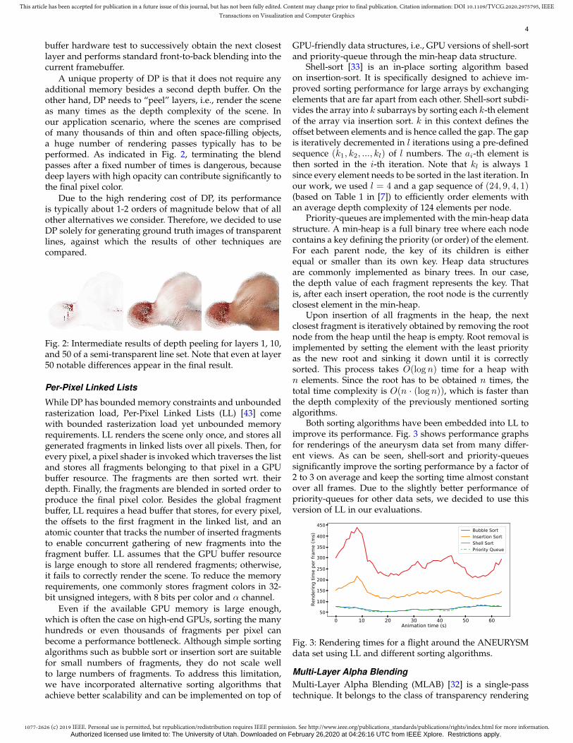
A unique property of DP is that it does not require anyadditional memory besides a second depth buffer. On theother hand, DP needs to “peel” layers, i.e., render the sceneas many times as the depth complexity of the scene. Inour application scenario, where the scenes are comprisedof many thousands of thin and often space-filling objects,a huge number of rendering passes typically has to beperformed. As indicated in Fig. 2, terminating the blendpasses after a fixed number of times is dangerous, becausedeep layers with high opacity can contribute significantly tothe final pixel color.

Due to the high rendering cost of DP, its performanceis typically about 1-2 orders of magnitude below that of allother alternatives we consider. Therefore, we decided to useDP solely for generating ground truth images of transparentlines, against which the results of other techniques arecompared.

Fig. 2: Intermediate results of depth peeling for layers 1, 10,and 50 of a semi-transparent line set. Note that even at layer50 notable differences appear in the final result.

Per-Pixel Linked Lists

While DP has bounded memory constraints and unboundedrasterization load, Per-Pixel Linked Lists (LL) [43] comewith bounded rasterization load yet unbounded memoryrequirements. LL renders the scene only once, and stores allgenerated fragments in linked lists over all pixels. Then, forevery pixel, a pixel shader is invoked which traverses the listand stores all fragments belonging to that pixel in a GPUbuffer resource. The fragments are then sorted wrt. theirdepth. Finally, the fragments are blended in sorted order toproduce the final pixel color. Besides the global fragmentbuffer, LL requires a head buffer that stores, for every pixel,the offsets to the first fragment in the linked list, and anatomic counter that tracks the number of inserted fragmentsto enable concurrent gathering of new fragments into thefragment buffer. LL assumes that the GPU buffer resourceis large enough to store all rendered fragments; otherwise,it fails to correctly render the scene. To reduce the memoryrequirements, one commonly stores fragment colors in 32-bit unsigned integers, with 8 bits per color and α channel.

Even if the available GPU memory is large enough,which is often the case on high-end GPUs, sorting the manyhundreds or even thousands of fragments per pixel canbecome a performance bottleneck. Although simple sortingalgorithms such as bubble sort or insertion sort are suitablefor small numbers of fragments, they do not scale wellto large numbers of fragments. To address this limitation,we have incorporated alternative sorting algorithms thatachieve better scalability and can be implemented on top of

GPU-friendly data structures, i.e., GPU versions of shell-sortand priority-queue through the min-heap data structure.

Shell-sort [33] is an in-place sorting algorithm basedon insertion-sort. It is specifically designed to achieve im-proved sorting performance for large arrays by exchangingelements that are far apart from each other. Shell-sort subdi-vides the array into k subarrays by sorting each k-th elementof the array via insertion sort. k in this context defines theoffset between elements and is hence called the gap. The gapis iteratively decremented in l iterations using a pre-definedsequence (k1, k2, ..., kl) of l numbers. The ai-th element isthen sorted in the i-th iteration. Note that kl is always 1since every element needs to be sorted in the last iteration. Inour work, we used l = 4 and a gap sequence of (24, 9, 4, 1)(based on Table 1 in [7]) to efficiently order elements withan average depth complexity of 124 elements per node.

Priority-queues are implemented with the min-heap datastructure. A min-heap is a full binary tree where each nodecontains a key defining the priority (or order) of the element.For each parent node, the key of its children is eitherequal or smaller than its own key. Heap data structuresare commonly implemented as binary trees. In our case,the depth value of each fragment represents the key. Thatis, after each insert operation, the root node is the currentlyclosest element in the min-heap.

Upon insertion of all fragments in the heap, the nextclosest fragment is iteratively obtained by removing the rootnode from the heap until the heap is empty. Root removal isimplemented by setting the element with the least priorityas the new root and sinking it down until it is correctlysorted. This process takes O(log n) time for a heap withn elements. Since the root has to be obtained n times, thetotal time complexity is O(n · (log n)), which is faster thanthe depth complexity of the previously mentioned sortingalgorithms.

Both sorting algorithms have been embedded into LL toimprove its performance. Fig. 3 shows performance graphsfor renderings of the aneurysm data set from many differ-ent views. As can be seen, shell-sort and priority-queuessignificantly improve the sorting performance by a factor of2 to 3 on average and keep the sorting time almost constantover all frames. Due to the slightly better performance ofpriority-queues for other data sets, we decided to use thisversion of LL in our evaluations.

Fig. 3: Rendering times for a flight around the ANEURYSMdata set using LL and different sorting algorithms.

Multi-Layer Alpha BlendingMulti-Layer Alpha Blending (MLAB) [32] is a single-passtechnique. It belongs to the class of transparency rendering




5

techniques that are bounded in both memory consump-tion and rendering load. This class of techniques does notperform exact visibility sorting of fragments but strives toapproximate the transmittance and color. MLAB does thisby heuristically merging fragments into a small number oflayers, a so-called blending array, that are finally mergedinto the pixel color.

The blending array consists of k buffers, into whichincoming fragments are merged. Each of the k buffers storesthe blended colors and transmittances of the fragmentsmerged into it, as well as a depth value. Each fragment isplaced into a corresponding buffer based on its depth. Whenall layers are occupied and the current fragment createsa new layer, the two most appropriate adjacent layers aremerged in turn.

We chose MLAB because of its simplicity, performance,and low memory consumption. On the other hand, it is clearthat with only k layers—eight by default in our currentimplementation—MLAB is not always able to accuratelyreconstruct the colors and transmittances for scenes withhigh depth complexity. In particular, the quality of MLABis highly dependent on the order in which fragments aregenerated, as the outcome of the heuristic merge operationdepends highly on this order. Some of the inaccuraciesshown in Fig. 1 are due to this dependency.

Additionally, MLAB is not frame-to-frame-coherent ifthe order in which fragments are rendered to the inter-mediate buffers is not guaranteed over time, resulting inflickering artifacts during animation. We prevent this errorby explicitly enabling order-preserving pixel synchroniza-tion (see [11]) so that fragments are processed in the orderprimitives were issued. Note that with pixel synchronizationenabled, we did not experience any loss or increase inperformance.

Multi Layer Alpha Blending with Depth BucketingTo make MLAB less dependent on the order in which frag-ments are generated, we propose a variant that considers adiscrete set of depth intervals. We call this approach MLABwith depth bucketing (MLABDB). The general idea underly-ing MLABDB is to discretize the scene into k disjoint bucketsthat perform MLAB independently for the correspondingdepth interval. Each fragment is thus assigned to a bucketby means of its depth value and merged heuristically intothe local corresponding color and transmittance buffer. Sincethe buckets are already sorted wrt. depth, blending canfinally be performed by blending the buckets’ values infront-to-back order.

However, only discretizing the scene into buckets ofequal intervals produced images with less quality and vis-ible artifacts. MLAB itself is not order-independent andyields different results per pixel depending on the order offragments for each bucket and pixel, resulting in artifacts.To avoid these artifacts, in MLABDB we segment the sceneinto two buckets and set the boundaries of the bucketsheuristically with respect to opacity (compare Fig. 4).

MLABDB requires two rendering passes to obtain thefinal color. In the first pass, the boundaries of the twobuckets are determined. For each gathered fragment, thefirst fragment with opacity α greater or equal a user-definedthreshold τα is maintained. The depth value zmin of this

1

0

Front Bucket Back Bucket Discarded

Fig. 4: Fragments with opacity, ordered by depth. MLABDBsearches for the first fragment with α ≥ τα to obtain depthboundary zmin of the front bucket. Back bucket bounds arezmin and zo, with zo the depth of the first opaque fragment.Fragments with z > zo are discarded.

fragment represents the upper depth boundary for the firstbucket, called front bucket. Since fragments behind opaquelines should not be merged the first opaque fragment withα ≥ τo is preserved. Its depth values zo and zmin definethe upper and lower boundary of the second bucket, calledthe back bucket. In the second pass, all incoming fragmentsare assigned to the corresponding bucket by using theirdepths, and heuristic merges are performed independentlyfor each bucket. Fragments with a depth value greater thanzo are discarded. For the front bucket, we found that n = 1or n = 2 layers were suitable to gather the fragmentsand avoid order-dependent problems of MLAB, under theassumptions that all fragments of low opacity contributeequally to the image. The back bucket uses a blending arraywith four or five layers. As demonstrated in Fig. 1c andfurther evaluated in Sec. 4, MLABDB can, in many cases,considerably improve the quality of MLAB (compare Fig. 5).On the other hand, since it requires more operations, it isslightly less efficient than MLAB. Note that thresholds needto be set carefully, as visual artifacts can occur as seen inFig. 11(a) and discussed in Sec. 4.5.

Fig. 5: Difference between MLAB (left) and our modifiedvariant MLABDB (right). MLAB reveals interior lines er-roneously due to wrong blending order. MLABDB renderscorrectly in this scenario.

Moment-Based Order Independent TransparencyMoment-Based Order Independent Transparency (MBOIT)[25] is another variant of transparency rendering techniqueswith bounded memory and rendering constraints. It buildsupon either power moments or trigonometric momentsto approximate the transmittance function per pixel in astochastic way. Power moments are used in statistics toreconstruct or approximate functions such as the mean andstandard deviation of arbitrarily sampled random distribu-tions. In addition, MBOIT operates on the logarithm of the




6

transmittances per fragment to enable order-independentadditive blending. The transmittance of the n-th fragmentat depth zf and opacity αf is given by

T (zf ) =n−1∏l=0

(1− αl), zl < zf (1)

The absorbance can then be defined in the logarithmicdomain as

A(zf ) = − lnT (zf ) =n−1∑l=0

−ln(1− αl) (2)

The absorbance can be interpreted as a cumulative distribu-tion function of the transmittance at each layer, given thatfor all l translucent fragments it holds that zl < zf . Thedistribution can be described as

Z :=n−1∑l=0

−ln(1− αl) · δzl , (3)

where δzl is the Dirac-δ function. Using a power mo-ments generating function b: [−1, 1] → Rm+1, b(z) =(1, z, z2, z3, · · · , bm)T , for m power moments the transmit-tance is given by

b := Ez(b) =n−1∑l=0

−ln(1− αl) · b(zl). (4)

MBOIT requires two passes to compute the final color. Inthe first pass, the m power moments are computed that arerequired to reconstruct the transmittance function. The firstpass requires storing m floating point values per pixel, weuse four in our experiments. In the second rendering pass,the transmittance of each fragment is reconstructed usingthe pre-computed power moments via

T (zf , b) = exp(−A(zf , b)). (5)

The real absorbance of the fragment is estimated by com-puting its lower and upper bounds and interpolating in-between these bounds with an interpolating factor β = 0.1.This factor was determined by testing multiple values andsettling for the one giving the best results. As the qualityof reconstruction further degrades with large depth valueranges, the depth values are transformed to logarithmicscale [25]. The final color can then be computed using thetotal absorbance, stored in the first power moment b0, andthe reconstructed transmittance T (zf , b) (cf. eq. 2 in [25]).

Munstermann et al. [25] pointed out that this is problem-atic for scenes with intersecting geometry and large depthranges, and this turns out to be especially problematic in thesituation where many changes in the transparencies alongone single view ray occur (see discussion in Sec. 4.5).

3.2 Image-OrderImage-order techniques guarantee exact visibility order ofthe surface points along the view rays. They utilize a searchstructure to efficiently find the objects that need to be tested.Therefore, they often come with increased, yet per-frameconstant memory requirements. On the other hand, theyhave unbounded rendering constraints, since the number ofray-object intersection tests depends on the view direction.

Voxel-Based Ray-CastingVRC is an image-order line rendering technique. It buildsupon the voxelization of a line set into a regular voxel gridand performs ray-casting in this grid with analytical ray-tube intersections to correctly blend all intersection points.For discretizing the lines into the voxel grid (i.e., curve vox-elization), each line is subdivided into a set of line segmentsby clipping the line at the voxel boundaries (see Fig. 6).To obtain a compact representation of these segments, theirendpoints are quantized based on a uniform subdivision ofthe voxel faces (i.e., line discretization).

Fig. 6: The original curve (red dotted line) is discretizedinto a voxel grid of 1, 4, and 16 voxels, respectively, fromleft to right. Per voxel lines are clipped against the voxelfaces and linearly connected. The blue curve represents theapproximated original curve at the given grid resolution.

For every pixel, a ray is cast through the voxel grid, go-ing from voxel face to voxel face using a digital differentialanalyzer algorithm. Whenever a voxel is hit, it is determinedhow many lines are stored in that voxel. If a voxel is empty,it is skipped; otherwise, the ray is intersected against thetubes corresponding to each line. If multiple intersectionswith the tubes are found, they are computed and thensorted in place in the correct visibility order. Since tubes canoverlap into adjacent voxels, neighboring voxels also needto be taken into account for intersection testing.

A potential weakness of VRC is the approximationquality. Curve voxelization and line quantization introducean approximation error, which increases with decreasinggrid resolution and coarser discretization of voxel faces.Conversely, higher grid resolutions and finer discretizationsyield better approximations, but can significantly increasethe memory required to store the voxel representation.

OSPRay CPU Ray TracingOSPRay is used to evaluate the performance of CPU ray-tracing for transparent line rendering. Within OSPRay, thereare three options for representing line primitives. OSPRay’sbuilt-in streamlines represent the lines as a combinationof analytic cylinder and sphere primitives, suitable forrendering opaque streamlines with a constant radius. Forsmoother higher-order curves or transparency, OSPRay canalso use Embree’s built-in Bezier curve primitive directly.Finally, the Generalized Tube Primitive module [13] extendsOSPRay’s original streamline approach to support varyingradii, bifurcations, and correct transparency. The General-ized Tubes module represents the streamlines as a combina-tion of spheres, cylinders and cone stumps, and employsa constructive solid geometry intersection test to ensurecorrect transparency. Although this CSG-based intersectioncomes at some cost, it is required to avoid showing interiorsurfaces from intersections with the constituent primitives.




7

To render the primitives, we use OSPRay’s built-in scientificvisualization renderer, which supports illumination effectssuch as shadows and ambient occlusion.

It is of course also possible to tessellate the tube prim-itives and render them in OSPRay as a triangle mesh. Inour testing, we found that when using a very low-qualitytessellation, the triangle mesh outperformed the General-ized Tubes for transparent geometry, due to the removalof the CSG traversal. However, even with a low-qualitytessellation, the memory consumed by the triangle meshis of concern, moreover, tessellating to a level of detailthat matches the quality of the Generalized Tubes or Beziercurves will require significantly more primitives, impactingperformance. For small- to medium- sized data sets, trian-gulation may be a reasonable approach.

RTX Ray TracingRTX is used to evaluate the performance of GPU ray-tracing for line rendering. On the RTX architecture, ded-icated hardware, the RT cores, are used to accelerate thetraversal of bounding volume hierarchies—utilizing axis-aligned bounding boxes—and the execution of ray-triangleintersection tests.

As the maximum recursion depth on current RTX hard-ware (32) is too low for data sets with high depth complex-ity, we opted for an iterative approach. We also note that arecursive approach is likely to be far more expensive thanan iterative one. Our first approach used any hit shadersto accumulate fragments along the rays. However, this canprovide only an approximate result, as any hit shaders arenot guaranteed to be run in a strict front-to-back order. Thus,we did not pursue this approach further.

Instead, in our experiments we utilize a closest hit shaderin combination with a loop in the ray generation shader thatblends the fragments returned by it in front-to-back order(cf. Fig. 7). Intersection sorting is thus done entirely by theacceleration structure traversal unit.

The closest hit shader also returns its hit distance alongthe ray, so that the ray generation shader can start thenext ray right after the last hit using a very small offsetto avoid intersecting the same primitive again. The loop isterminated by either a sentinel value returned from the missshader, run when no primitive is hit, or a zero transmittancevalue. Although iterative next-hit traversals could, in theory,fail to find all intersection hits (see Wald et al. [36]), we havenot experienced this problem in our experiments.

The RTX framework can also trace against custom ge-ometry using an intersection shader, which we utilize toperform analytic intersection tests against the tube represen-tations for each line. A ray is first intersected with an infinitetube, and the intersection points are then clipped againstthe two planes delimiting the tube segment. To correctlyinterpolate the vertex attributes in the closest hit shader,both planes are intersected with a line parallel to the tubeand through the clipped point. The position of the clippedpoint on this line segment is then mapped to [0; 1] and usedas interpolation factor in the closest hit shader.

Interestingly, the analytic ray intersection tests are abouta factor of two slower than ray-triangle intersection tests,even though the lower primitive count leads to a signifi-cantly smaller memory footprint. The high performance for

Ray Generation

Shader

Blending

Hit

TraceRay()

DispatchRays()

d

Fig. 7: Illustration of iterative ray-casting using the RTXframework. Blue-colored paths represent line primitives ofthe data set. At each frame, the ray generation shaderis called once and is responsible for iteratively blendingover all fragments and issuing new rays (TraceRay()) atintersection point ti (green arrows). During ray traversal,the intersection point with primitive closest to the viewer iscomputed. On each hit, color and opacity of line is obtainedand sent back to the ray generation shader (orange arrows).

triangles is likely attributable to the hardware accelerationof triangle intersection testing on the RTX hardware, anddo not consider analytical tests in the remainder of theevaluation for RTX.

4 EVALUATION

We evaluate and compare all selected line rendering tech-niques regarding memory consumption, performance, andquality. All GPU techniques were run on a standard desktopPC with Intel Xeon processor, 32 GB RAM, and an NVIDIAGeforce TITAN RTX with 24 GB VRAM. CPU ray-tracingwas performed on a system with 2 Intel Xeon E5-2640CPUs at 2.4 GHz and 3.4 GHz boost frequency with 40CPU threads in total. We used the Vulkan SDK 1.1.129with the extension VK NV ray tracing to implement RTXray tracing and conducted the performance tests using theNVIDIA driver 441.87. Both CPU and GPU architecturescome at roughly the same price, making the comparison fairin terms of financial investment. Furthermore, all perfor-mance measurements (using data sets that fit into memory)were carried out on an NVIDIA Geforce RTX 2060 SUPERwith 8 GB VRAM and a single Intel i7-5930K CPU with12 threads. The performance scale-down compared to themeasurements in Sec. 4.4 was roughly a factor of 1.6 – 3and 2, respectively. All images were rendered at a viewportresolution of 1920×1080 for performance and 1280×720 forimage quality. When statistics are given for flights around adata set, the camera parameters were set so that most of theviewport is covered by that data set and the entire viewportis covered in zoom-in scenarios. Ground truth images aregenerated via DP, yet we do not consider DP any furtherdue to the limitations discussed in the introduction.

4.1 Data Sets

Our experiments were performed on data sets with vastlydifferent numbers of lines and line density. For each data set,we selected meaningful transparency assignments, e.g., bymapping physical parameters along the lines or geometricline curvature to transparency. The following data sets wereused:

• ANEURYSM: 9,200 randomly seeded streamlines inthe interior of an aneurysm [5], and advected up to




8

Fig. 8: Data sets used in our experiments. Top: Opaque line rendering. Bottom: Transparent line rendering. From leftto right: ANEURYSM, CONVECTION, TURBULENCE, and CLOUDS. Transparency greatly aids the ability to visualizeimportant features in the data.

the vascular wall. Vorticity in the flow field fromwhich the lines were extracted is mapped to linetransparency.

• CONVECTION: 100,000 short streamlines that wereuniformly seeded in a Rayleigh-Bernard convec-tion between a heated bottom wall and a cold topwall [28]. Transparency is assigned according to linecurvature.

• TURBULENCE: 80,000 long streamlines generatedin a forced turbulence field of resolution 10243 [2].Transparency is proportional to the maximum λ2vortex measure along a line.

• CLOUDS: 400,000 seeded streamlines in a cloud-resolving boundary layer simulation (UCLA-LES, see[34]) using a large eddy simulation (LES). Streamlineintegration was conducted on a voxel grid withresolution 384×384×130. The magnitude of vorticityalong each streamline is mapped to transparency.

Fig. 8 shows all data sets, rendered via opaque andtransparent lines. Most data sets are very dense, yet bymapping the selected parameters linearly to transparency,important interior structures can be revealed. Table 1 givesfurther information on the number of line segments thatneed to be rendered as tubes, the memory that is required bythe initial line representation, and the memory requirementsof the internal data representation used by each technique,as explained in the next subsection.

4.2 Data Preparation and Model RepresentationAll rasterization-based line rendering techniques and RTXrender the tubes as triangle meshes. Therefore, each con-nected sequence of lines first needs to be converted intoa set of triangulated tubes that are stitched together toform a closed mesh. This pre-process is performed on theGPU. The meshes are stored in a triangle and shared vertexrepresentation with normal buffer, where each index andvector component is represented by a 32-bit value. In anadditional attribute buffer, 16-bit per-vertex attribute valuesare stored. During rendering, these values are mapped totransparency and color. To construct the tubes, for everyvertex shared by two lines, the average of the lines’ tangentvectors is computed. At the first and last vertex, respectively,the average is just the tangent of the first and last line

segment. Three vertices are generated and placed uniformlyon a circle around the vertex in the plane orthogonal to theaverage tangent and containing this vertex. The three ver-tices from the line start and end points are then connected toform a closed set of tubes. We use the same circle radius forall tubes. The vectors from the initial vertex to the new onesare used as per-vertex normals. From our experiments, wefound that three vertices along a circle radius are sufficientto achieve good results from each view direction.

The resulting buffers are used directly as input forLL, MLAB, MBOIT, and RTX. It is worth noting that allrasterization-based techniques can also generate the poly-gon models on the fly during rendering in a geometryshader, or use a pixel shader that takes the line informa-tion as input and analytically tests for intersections withthe corresponding tube. However, since rendering the pre-computed geometry is up to a factor of 2 faster, we do notconsider on the fly generation in our evaluation.

RTX requires another pre-process to build an AABB hier-archy from the given polygon model. For triangle geometry,the RTX framework supports only a few position formats,and raw data must be converted if it does not alreadymatch. For custom geometry, the API requires conservativeestimates of the AABB of each primitive. Construction of theAABB hierarchy is performed on the GPU via the API. RTXthen generates a tree structure, that is traversed by everyray until reaching the leaf nodes where ray-triangle tests areperformed.

Since VRC cannot handle polygon models but tests ana-lytically against the tubes during ray-casting, a voxel-basedrenderable line representation is first built and uploaded tothe GPU. For ANEURYSM and CONVECTION, we usedan optimized voxel grid resolution of 113×110×128 (x,y,z-dimension) and 128×8×128, respectively, and a quantiza-tion level of 16. For TURBULENCE and CLOUDS, weincreased the resolutions to 2563 and 5123, respectively, andused a quantization level of 32. Grid resolutions were chosento reduce the probability that lines fall onto each other andbecome indistinguishable.

OSP constructs a bounding volume hierarchy using Em-bree [40]. From the input line data, we build the GeneralizedTubes geometry, which consists of a set of analytic spheres,cylinders, and cone stumps, the union of which forms thetube. These primitives are passed to Embree as a user




9

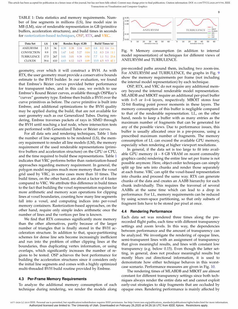
TABLE 1: Data statistics and memory requirements. Num-ber of line segments in millions (LS), line model size inMB (LM), size of renderable representation in GB (primitivebuffers, acceleration structures), and build times in secondsfor rasterization-based techniques, OSP, RTX, and VRC.

Data Set LS LM Render. Repr. (GB) Build Times (s)

ANEURYSM 2.3 34 0.39 0.38 2.04 0.05 0.8 0.2 0.6 3.6

CONVECTION 9.9 151 1.67 1.62 5.27 0.04 3.2 0.3 2.8 11.1

TURBULENCE 17.5 267 3.01 3.01 9.38 0.50 7.7 1.1 5.1 23.6

CLOUDS 39.6 610 4.63 6.12 14.5 0.89 13.5 4.5 9.5 42.1

geometry, over which it will construct a BVH. As withRTX, the user geometry must provide a conservative boundsestimate to the BVH builder. In our evaluation, we foundthat Embree’s Bezier curves provided better performancefor transparent tubes, and in this case, we switch to useEmbree’s Round Bezier curves, available through OSPRay’s“curves” geometry type. Embree then builds a BVH over thecurve primitives as before. The curve primitive is built intoEmbree, and additional optimizations to the BVH qualitymay be applied during the build, that are not available foruser geometry such as our Generalized Tubes. During ren-dering, Embree traverses packets of rays in SIMD throughthe BVH until reaching a leaf node, where intersection testsare performed with Generalized Tubes or Bezier curves.

For all data sets and rendering techniques, Table 1 liststhe number of line segments to be rendered (LS), the mem-ory requirement to render all line models (LM), the memoryrequirement of the used renderable representations (primi-tive buffers and acceleration structure) on the GPU or CPU,and the time required to build these representations. Table 1indicates that VRC performs better than rasterization-basedapproaches regarding memory requirement. In general, thepolygon model requires much more memory than the voxelgrid used by VRC, in some cases more than 10 times. Thebuild times, on the other hand, are about a factor of 4 fastercompared to VRC. We attribute this difference in build timesto the fact that building the voxel representation requires farmore arithmetic and memory scan operations for clippinglines at voxel boundaries, counting how many line segmentsfall into a voxel, and computing indices into per-voxelmemory containers. Rasterization-based approaches, on theother hand, require only simple index arithmetic once thenumber of lines and the vertices per line is known.

We find that RTX consumes significantly more memorythan the other alternatives, partly because of the largernumber of triangles that is finally stored in the BVH ac-celeration structure. In addition to that, space-partitioningschemes for dense line sets become increasingly inefficientand run into the problem of either clipping lines at theboundaries, thus duplicating vertex information, or usingoverlaps, which significantly increases the number of re-gions to be tested. OSP achieves the best performance forbuilding the acceleration structures since it considers onlythe initial line segments and comes with a highly optimizedmulti-threaded BVH build routine provided by Embree.

4.3 Per-Frame Memory RequirementsTo analyze the additional memory consumption of eachtechnique during rendering, we render the models along

0 10 20 30 40 50 60Animation time (s)

0.03

0.10

1.002.004.00

Tota

l mem

ory

Cons

umpt

ion

(GB)

ANEURYSM

0 10 20 30 40 50 60Animation time (s)

0.03

0.10

1.002.004.00

Tota

l mem

ory

Cons

umpt

ion

(GB)

LLMBOITMLABDBVRCRTXOSP

TURBULENCE

Fig. 9: Memory consumption (in addition to internalmodel representation) of techniques for different views ofANEURYSM and TURBULENCE.

pre-recorded paths around them, including two zoom-ins.For ANEURYSM and TURBULENCE, the graphs in Fig. 9show the memory requirements per frame (not includingthe internal model representation) by each technique.

OSP, RTX, and VRC do not require any additional mem-ory beyond the internal renderable model representation.MLABDB and MBOIT require an additional per-pixel bufferwith k=5 or k=4 layers, respectively. MBOIT stores four32-bit floating point power moments in these layers. Thememory consumption of this buffer is negligible comparedto that of the renderable representation. LL, on the otherhand, needs to keep a buffer with as many entries as themaximum number of fragments that can be generated forany of the possible views. Due to performance issues, thisbuffer is usually allocated once in a pre-process, using aprescribed maximum number of fragments. The memoryconsumption of LL can exceed the available GPU memory,especially when rendering at higher viewport resolutions.

In general, if the data set is too large to fit into avail-able GPU memory (4 – 8 GB VRAM on recent commoditygraphics cards) rendering the entire line set per frame is notpossible anymore. Here, object-order techniques can simplysplit up line sets into chunks and render those separatelyat each frame. VRC can split the voxel-based representationinto chunks and proceed the same way. RTX can generatechunks of the data and creates an AABB hierarchy for eachchunk individually. This requires the traversal of severalAABBs at the same time which can lead to a drop inperformance. For LL, memory requirements can be reducedby using screen-space partitioning, so that only subsets offragment lists have to be stored per pixel at once.

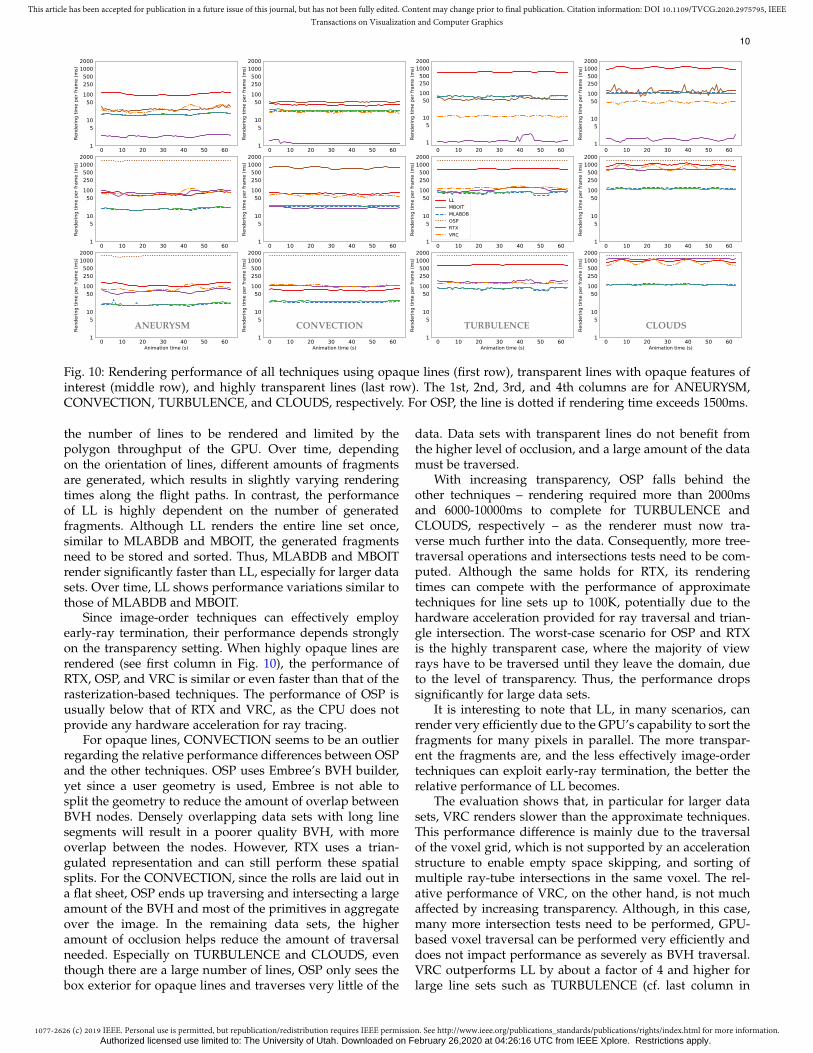
4.4 Rendering PerformanceEach data set was rendered three times along the pre-recorded flight paths, each time with different transparencysettings and zoom levels. In this way, the dependenciesbetween performance and the amount of transparency canbe analyzed. We investigate the rendering of opaque lines,semi-transparent lines with an assignment of transparencythat gives meaningful results, and lines with constant lowtransparency (e.g. below 0.15). Even though the latter set-ting, in general, does not produce meaningful results butmostly blurs out directional information, it is used todemonstrate how either technique behaves in this worst-case scenario. Performance measures are given in Fig. 10.

The rendering times of MLABDB and MBOIT are almostconstant for different transparency settings since both tech-niques always render the entire data set and cannot exploitearly-out strategies to skip fragments that are occluded byopaque ones. Rendering performance is mainly affected by




10

0 10 20 30 40 50 60Animation time (s)

1

510

50100250500

10002000

Rend

erin

g tim

e pe

r fra

me

(ms)

0 10 20 30 40 50 60Animation time (s)

1

510

50100250500

10002000

Rend

erin

g tim

e pe

r fra

me

(ms)

0 10 20 30 40 50 60Animation time (s)

1

510

50100250500

10002000

Rend

erin

g tim

e pe

r fra

me

(ms)

0 10 20 30 40 50 60Animation time (s)

1

510

50100250500

10002000

Rend

erin

g tim

e pe

r fra

me

(ms)

0 10 20 30 40 50 60Animation time (s)

1

510

50100250500

10002000

Rend

erin

g tim

e pe

r fra

me

(ms)

0 10 20 30 40 50 60Animation time (s)

1

510

50100250500

10002000

Rend

erin

g tim

e pe

r fra

me

(ms)

0 10 20 30 40 50 60Animation time (s)

1

510

50100250500

10002000

Rend

erin

g tim

e pe

r fra

me

(ms)

LLMBOITMLABDBOSPRTXVRC

0 10 20 30 40 50 60Animation time (s)

1

510

50100250500

10002000

Rend

erin

g tim

e pe

r fra

me

(ms)

0 10 20 30 40 50 60Animation time (s)

1

510

50100250500

10002000

Rend

erin

g tim

e pe

r fra

me

(ms)

ANEURYSM

0 10 20 30 40 50 60Animation time (s)

1

510

50100250500

10002000

Rend

erin

g tim

e pe

r fra

me

(ms)

CONVECTION

0 10 20 30 40 50 60Animation time (s)

1

510

50100250500

10002000

Rend

erin

g tim

e pe

r fra

me

(ms)

TURBULENCE

0 10 20 30 40 50 60Animation time (s)

1

510

50100250500

10002000

Rend

erin

g tim

e pe

r fra

me

(ms)

CLOUDS

Fig. 10: Rendering performance of all techniques using opaque lines (first row), transparent lines with opaque features ofinterest (middle row), and highly transparent lines (last row). The 1st, 2nd, 3rd, and 4th columns are for ANEURYSM,CONVECTION, TURBULENCE, and CLOUDS, respectively. For OSP, the line is dotted if rendering time exceeds 1500ms.

the number of lines to be rendered and limited by thepolygon throughput of the GPU. Over time, dependingon the orientation of lines, different amounts of fragmentsare generated, which results in slightly varying renderingtimes along the flight paths. In contrast, the performanceof LL is highly dependent on the number of generatedfragments. Although LL renders the entire line set once,similar to MLABDB and MBOIT, the generated fragmentsneed to be stored and sorted. Thus, MLABDB and MBOITrender significantly faster than LL, especially for larger datasets. Over time, LL shows performance variations similar tothose of MLABDB and MBOIT.

Since image-order techniques can effectively employearly-ray termination, their performance depends stronglyon the transparency setting. When highly opaque lines arerendered (see first column in Fig. 10), the performance ofRTX, OSP, and VRC is similar or even faster than that of therasterization-based techniques. The performance of OSP isusually below that of RTX and VRC, as the CPU does notprovide any hardware acceleration for ray tracing.

For opaque lines, CONVECTION seems to be an outlierregarding the relative performance differences between OSPand the other techniques. OSP uses Embree’s BVH builder,yet since a user geometry is used, Embree is not able tosplit the geometry to reduce the amount of overlap betweenBVH nodes. Densely overlapping data sets with long linesegments will result in a poorer quality BVH, with moreoverlap between the nodes. However, RTX uses a trian-gulated representation and can still perform these spatialsplits. For the CONVECTION, since the rolls are laid out ina flat sheet, OSP ends up traversing and intersecting a largeamount of the BVH and most of the primitives in aggregateover the image. In the remaining data sets, the higheramount of occlusion helps reduce the amount of traversalneeded. Especially on TURBULENCE and CLOUDS, eventhough there are a large number of lines, OSP only sees thebox exterior for opaque lines and traverses very little of the

data. Data sets with transparent lines do not benefit fromthe higher level of occlusion, and a large amount of the datamust be traversed.

With increasing transparency, OSP falls behind theother techniques – rendering required more than 2000msand 6000-10000ms to complete for TURBULENCE andCLOUDS, respectively – as the renderer must now tra-verse much further into the data. Consequently, more tree-traversal operations and intersections tests need to be com-puted. Although the same holds for RTX, its renderingtimes can compete with the performance of approximatetechniques for line sets up to 100K, potentially due to thehardware acceleration provided for ray traversal and trian-gle intersection. The worst-case scenario for OSP and RTXis the highly transparent case, where the majority of viewrays have to be traversed until they leave the domain, dueto the level of transparency. Thus, the performance dropssignificantly for large data sets.

It is interesting to note that LL, in many scenarios, canrender very efficiently due to the GPU’s capability to sort thefragments for many pixels in parallel. The more transpar-ent the fragments are, and the less effectively image-ordertechniques can exploit early-ray termination, the better therelative performance of LL becomes.

The evaluation shows that, in particular for larger datasets, VRC renders slower than the approximate techniques.This performance difference is mainly due to the traversalof the voxel grid, which is not supported by an accelerationstructure to enable empty space skipping, and sorting ofmultiple ray-tube intersections in the same voxel. The rel-ative performance of VRC, on the other hand, is not muchaffected by increasing transparency. Although, in this case,many more intersection tests need to be performed, GPU-based voxel traversal can be performed very efficiently anddoes not impact performance as severely as BVH traversal.VRC outperforms LL by about a factor of 4 and higher forlarge line sets such as TURBULENCE (cf. last column in




11

Fig. 10). Again, for ANEURYSM and CONVECTION withmany empty regions that need to be traversed on the finestvoxel level, the relative performance of VRC compared tothe rasterization-based approaches decreases. For CLOUDS,traversing large voxel grids (5123) greatly reduces VRC’sperformance and leads to rendering times similar to LLwhen looking from a diagonal angle into the line set.

4.5 Image Quality

LL, VRC, OSP, and RTX simulate the effect of transparencyaccurately. VRC introduces errors due to the voxelizationand quantization of lines into a regular voxel grid; however,the visibility order of lines in the grid is handled correctly.In the worst-case, multiple lines can fall on top of each otherin the grid, resulting in an incorrect blending order. In ourexperiments, we did not perceive visual artifacts caused bythis effect.

Inaccuracies in MLAB are caused by lines that are notrendered in correct visibility order, and that are mergedheuristically using a limited number of transmittance layers.For scenes with high depth complexity, and even whenlow transparency is used, the accumulation of errors leadsto visible artifacts. Most prominent are errors caused byincorrect merging of fragments with high opacity, i.e., whentwo such fragments are merged in the wrong order into thesame transmittance layer (Fig. 1(c) and Fig. 5). If lines areby chance rendered in the correct visibility order, or fewopaque fragments are blended into different transmittancelayers, MLAB can nevertheless generate accurate results(see Fig. 1(a) for an example). The view-dependent natureof MLAB, i.e., errors can suddenly appear or disappeardepending on whether the rendering order matches thecurrent visibility order, makes it less time coherent.

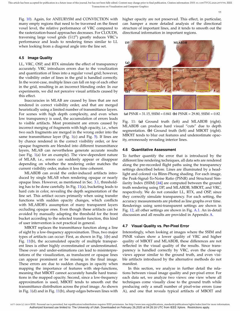
MLABDB can avoid the order-induced artifacts intro-duced by single MLAB when rendering opaque or nearlyopaque lines. However, as mentioned in Sec. 3.1, threshold-ing has to be done carefully. In Fig. 11(a), bucketing leads tohard cuts in color, revealing the depth segmentation of theline set. This artifact occurs primarily when using transferfunctions with sudden opacity changes, which conflictswith MLABDB’s assumption of many transparent layersoccluding opaque ones. Even though these artifacts can beavoided by manually adapting the threshold for the frontbucket according to the selected transfer function, this kindof user intervention is not practical in general.

MBOIT replaces the transmittance function along a lineof sight by a low-frequency approximation. Thus, two majortypes of artifacts can occur: First, as shown in Fig. 1(b) andFig. 11(b), the accumulated opacity of multiple transpar-ent lines is either highly overestimated or underestimated.These over- and under-estimations can lead to misinterpre-tations of the visualization, as translucent or opaque linescan appear prominent or be missing in the final image.These errors are due to sudden changes in opacity whenmapping the importance of features with step-functions,meaning that MBOIT cannot accurately handle hard transi-tions in the mapped opacity. Second, since a low-frequencyapproximation is used, MBOIT tends to smooth out thetransmittance distribution across the pixel image. As shownin Fig. 1(d) and in Fig. 11(b), sharp edges between lines with

higher opacity are not preserved. This effect, in particular,can hamper a more detailed analysis of the directionalstructure of important lines, and it tends to smooth out thedirectional information in important regions.

DP

(a)

MLABDB

DP

(b)

(a) PSNR = 31.15, SSIM = 0.841

MBOIT

(b) PSNR = 29.80, SSIM = 0.82

Fig. 11: (a) Ground truth (left) and MLABDB (right).MLABDB can produce hard visual “cuts” due to depthsegmentation. (b) Ground truth (left) and MBOIT (right).MBOIT tends to blur out features and underestimate opac-ity, erroneously revealing interior lines.

4.6 Quantitative Assessment

To further quantify the error that is introduced by thedifferent line rendering techniques, all data sets are renderedalong the pre-recorded flight paths using the transparencysettings described before. Lines are illuminated by a head-light and colored via Blinn-Phong shading. For each image,the Peak-Signal-To-Noise Ratio (PSNR) and Structural Sim-ilarity Index (SSIM) [44] are computed between the groundtruth rendering using DP, and MLABDB, MBOIT, and VRC,respectively. We do not consider LL, RTX, and OSP, sincethey correctly simulate transparency. For each setting, theaccuracy measurements are plotted as line graphs over time.Renderings using semi-transparent settings are shown inFig. 12, all other settings are shown in Fig. A.1. An in-detaildiscussion and all results are provided in Appendix A.

4.7 Visual Quality vs. Per-Pixel Error

Interestingly, when looking at images where the SSIM andPSNR values show a lower quality of VRC and higherquality of MBOIT and MLABDB, these differences are notreflected in the visual quality of the results. Since trans-parency is handled correctly by VRC, even the close-upviews appear similar to the ground truth, and even visi-ble artifacts introduced by the alternative methods do notmanifest.

In this section, we analyze in further detail the rela-tions between visual image quality and per-pixel error. Foreach data set, we analyze two views: one view where alltechniques come visually close to the ground truth whileproducing only a small number of pixel-wise errors (caseA), and one that reveals typical artifacts of MBOIT and




12

0 10 20 30 40 50 60Animation time (s)

0.6

0.7

0.8

0.9

1.0

SSIM

SSIM for semi-transparent lines over time

MBOITMLABDBVRCDP

0 10 20 30 40 50 60Animation time (s)

0.6

0.7

0.8

0.9

1.0

SSIM


0 10 20 30 40 50 60Animation time (s)

0.6

0.7

0.8

0.9

1.0

SSIM


0 10 20 30 40 50 60Animation time (s)

0.6

0.7

0.8

0.9

1.0

SSIM


0 10 20 30 40 50 60Animation time (s)

20

30

40

50

60

PSNR

PSNR for semi-transparent lines over time

ANEURYSM

0 10 20 30 40 50 60Animation time (s)

20

30

40

50

60

PSNR


CONVECTION

0 10 20 30 40 50 60Animation time (s)

20

30

40

50

60

PSNR


TURBULENCE

0 10 20 30 40 50 60Animation time (s)

20

30

40

50

60

PSNR


CLOUDS

Fig. 12: Error metrics of all techniques using transparent lines with opaque features of interest. The 1st, 2nd, 3rd, and 4thcolumns are for ANEURYSM, CONVECTION, TURBULENCE, and CLOUDS, respectively. The First row shows SSIM foreach technique, the second shows PSNR. A higher value is better.

MLABDB using a most meaningful transparency settingswith sharp transitions and alternating high transparencyand opacity (case B).

Besides an image-to-image comparison, the analysis isadditionally supported by visualizations of the absoluteper-pixel differences to the ground truth. These plots aregrayscale images with black regions highlighting large colordifferences. Significant differences in images are marked bycolored rectangles and supported by close-up views. Imagecomparisons of all cases (Fig. A.x) are given in Appendix A.

Fig. A.2 depicts a scenario where the viewer is lookingthrough the entire ANEURYSM data set with alternatingopaque lines (red-colored) and transparent lines (orange-ocher). For case A (cf. Fig. A.2(a), corresponding to frame5 of the first column in Fig. 12), we observe that alltechniques are close to the ground truth image with thebest image produced by MLABDB. MBOIT overestimatesthe transparency of few transparent fragments occludingopaque lines highlighted by per-pixel error plots (cf. blackregions in Fig. A.2(a) (MBOIT)). VRC produces high pixelerrors in regions close to the viewer since line inaccuraciesaffect larger areas of pixels. However, the quality of VRCbecomes better with larger distance to the camera, leadingto results indistinguishable from the ground truth. Wrt. caseB (cf. Fig. A.2(b)), the quality of both MBOIT and MLABDBis worse than VRC. MBOIT struggles to approximate sharptransitions in transparency leading to high over- and under-estimations, whereas MLABDB is not able to correctly mergeopaque fragments. Bucketing is impossible here, leading tovisual artifacts. However, VRC remains stable and, besidesline inaccuracies, is very close to the ground truth.

Another example is given in Fig. A.3 when looking froma diagonal angle into the entire CONVECTION line set, withthe number of transparent lines increasing with the distanceto the viewer. For case A (cf. Fig. A.3(a)), all techniques arevisually close to the ground truth with MLABDB workingbest. Here, MBOIT exhibits small errors in transmittanceapproximation, as many opaque lines are occluded bytransparent ones. These errors propagate towards the back-ground as the number of fragments increases with distance,leading to further image quality degradation. With opaquelines more present in this case, VRC produces a number

of wrong line silhouettes due to curve discretization, em-phasized in per-pixel error plots along the line edges. Forcase B, the quality of both MLABDB and MBOIT decreaseswith larger distance (cf. Fig. A.3(b)). In particular, MLABDBproduces more per-pixel color inconsistencies, depicted byhigh noise in error plots, toward the background as moreand more fragments are merged incorrectly. On the otherhand, MBOIT has difficulty coping with sharp transitionsbetween transparent and opaque fragments. Interestingly,the image quality of VRC is independent of the viewer’sdistance or angle, and line inaccuracies do not accumulatewith increasing distance.

Fig. A.4 demonstrates the differences of image quality forzoom-out and close-up views. Here, case A (cf. Fig. A.4(a))represents a zoom-out view that corresponds to frame eightof the third column in Fig. 12. All techniques are ableto properly render TURBULENCE and are visually indis-tinguishable from the ground truth, although MLABDBshows some weaknesses in rendering transparent regionsdue to incorrect fragment merges. However, these pixelerrors hardly affect the overall quality of the image. Wrt.VRC, line inaccuracies are not present here since lines arehighly transparent and line edges are not emphasized. CaseB (cf. Fig. A.4(b)) shows the impact of zoom-ins on thequality of all techniques. MLABDB properly renders opaquelines (red-colored tubes), but incorrectly merges fragmentsin regions with a large number of highly transparent lines,leading to a wrong colored region (orange instead of ocher)after blending. MBOIT is able to approximate transmittancein transparent regions but fails to display sharp opaque lineswhere opaque and transparent lines are close by, leading toblurred outline structures in the final image. Per-pixel errorplots for VRC reveal some line inaccuracies but demonstratethat, overall, a good image quality is achieved by VRC evenfor this large data set.

The last example demonstrates the impact of large, denseline data with many layers per pixel (> 10000 at maximum),using high transparency in Fig. A.5(a) and semi-transparentopacity settings in Fig. 13 and Fig. A.5(b). In the firstscenario, all techniques are able to properly render the dataset. However, MLABDB produces a few wrongly coloredfeatures due to false fragment merging. MBOIT works prop-




13

DP MBOIT

PSNR = 34.71, SSIM = 0.920

MLABDB

PSNR = 32.11, SSIM = 0.940

VRC

PSNR = 30.27, SSIM = 0.750

Fig. 13: From left to right: CLOUDS rendered with DP, MBOIT, MLABDB, VRC. Images show renderings using sharptransitions between low and high transparency. Blue and yellow rectangles highlight differences between techniques;close-up views are shown below each image.

erly for this case, and produces few over- or underestima-tions. VRC, on the other hand, tends to underestimate theactual transmittance as some lines fall into the same cell(disadvantage of VRC explained in Sec. 3.2). Weaknesses ofall techniques are even more pronounced in the second sce-nario; for example, there are more wrongly colored featuresproduced by MLABDB. Due to its line approximation, VRCalso struggles to fully reconstruct the actual transmittance.MBOIT works best for CLOUDS, as there are only a fewoverestimates of the actual transmittance.

Since MLABDB and MBOIT do not depend on anyprimitive type, we also investigated the image quality of ourproposed approximate techniques when rendering transpar-ent triangle surfaces and point cloud data. The visualizationof these types of data with transparency can, similar toline sets, lead to complex rendering scenarios with manytransparent layers and multiple occlusions. However, forthose data types, MLABDB and MBOIT showed similarcharacteristics as for line sets during rendering (see Ap-pendix B).

In summary, although all techniques show weaknessessome weaknesses in some cases resulting in pixel-errors,they are able to render transparent data sets with high depthcomplexity at high image quality. Moreover, OSP, RTX, andVRC are temporally stable for all transparency settings anddata sets. VRC, despite line inaccuracies, comes very closeto the ground truth.

5 DISCUSSION

In the following sections, we discuss the major characteris-tics of all rendering techniques, as given in Tab. 2 and alsopresent the outcome of an informal user study to shed lighton the perception of the errors that are introduced by object-order approximate techniques.

5.1 Object-OrderEquipped with dedicated GPU-friendly sorting algorithmsand data structures, LL shows good rendering performancefor all but the largest data sets. LL was never slower than afactor of 4-5 compared to approximate techniques for smalldata sets. For dense data sets with high depth complexityof more than a thousand layers, however, the required GPUbuffers can easily exceed available GPU memory, especiallyfor resolutions above 1080p.

Approximate rasterization-based techniques are veryfast, work with rendering constraints, and support render-ing on hardware with bounded memory. Rendering con-straints for MLABDB and MBOIT involve, for each pixel,the maximum number of fragments stored or model param-eters to approximate the transmittance function. These con-straints implicitly keep the memory consumption constantover time.

MLABDB and MBOIT provide good quality in manyreal-world scenarios, particularly in scenes where featuresof interest are rendered opaque and remaining lines aremapped to high transparency. Introduced artifacts are oftensubtle and local, yet in some views they can cause artifactsthat even give a wrong understanding of the line structures.Approximate techniques also fail to maintain time coher-ence, as their per-pixel rendering outcome is dependent onthe transmittance function along each pixel. These errors areespecially frequent if high-frequency transfer functions fortransparency are used, which can lead to distracting render-ing artifacts. Although approximation errors can be reducedby, i.e., increasing the number of nodes of MLABDB’s blend-ing arrays (in example to more than 15 layers) or the numberof power moments, such settings considerably reduce ren-dering performance and increase memory consumption.

Informal User Study

In a simple user study, users were asked to give theirassessment of the quality differences between MLABDB andMBOIT, to further shed light on the perceptional differencesbetween these approximate variants. We recruited 24 par-ticipants, comprised of 19 computer science students and 5computer science PhD students, all having a background incomputer graphics. The participants were selected to haveno color vision deficiency. The students were exposed to theapplication of line rendering for the first time. None of themknew the visualized vector fields and line sets beforehand.The study was performed using the desktop PC describedabove. We showed the users the tool and let them work witha data set not included in the study. Then, we performed twodifferent experiments:

• To each user, we showed a sequence of eight tri-setsof renderings: the ground truth image first, and thenthe same view rendered with MLABDB and MBOIT(showing their typical artifacts) side by side.




14

TABLE 2: Comparison table of all techniques wrt. type of order, render accuracy, performance, render constraints (RenderC),support of bound memory (BoundM), temporal coherency (Temp), changes in color along each pixel (ChColor), dense(large) data sets (Dense), semi-transparent transparency settings (STrans), and support of global illumination (GI) effects.Symbols + and – represent high or low performance/quality, respectively (two repeating symbols indicate very high / verylow performances). / represents ratings for opaque / semi-transparent (left) and highly transparent lines (right).

Technique Order Accuracy Perform. RenderC BoundM Temp ChColor Dense STrans GI

DP Object Exact – – 8 4 4 + + – – + + 8

LL Object Exact +/– 8 8 4 + + – – + + 8

MLABDB Object Approx. + + 4 4 8 – – + 8

MBOIT Object Approx. + + 4 4 8 –/+ + – 8

VRC Image Approx. +/– 4 4 4 + + – + + 4

OSP Image Exact. +/– – 8 8 4 + + – – +/– 4

RTX Image Exact + +/– 8 8 4 + + +/– + + 4

• Each user carried out three interactive sessions withtwo data sets, one minute each. First, the same dataset was visualized, starting with MLABDB and thenusing MBOIT; then the experiment was repeated inreverse order using a different data set.

Users were then asked to rate the visual quality of thestill images and the animations. For both experiments, userscould select either MBOIT or MLABDB as the best, or“undecided”. We had three renderings where 70% of theusers selected MBOIT, three renderings where 63% selectedfor MLAB, and two renderings where 65% of the users wereundecided. In addition to the comparison of MBOIT andMLABDB, we asked the users to rate the image qualityof still images as “no difference” (good) to the groundtruth, “acceptable” (acc), or “non-acceptable” (non-acc). ForMBOIT, 41% rated it as good, 46% as acceptable, and 13%as non-acceptable. For MLABDB, 44% rated it as good, 32%as acc, and 24% as non-acc. To assess the image qualityover time for each technique, we asked users in a secondexperiment to rate the quality of the videos similar to imagequality. For MBOIT, 62% rated it as good quality, 35% asacceptable quality, and 3% as non-acc. For MLABDB, 45%of users rated it as good, 47% as acc, and 8% as non-acc.

About why they scored the renderings as good, accept-able, or non-acceptable, users mentioned that wrong coloroutputs and rendering order artifacts (line features falselyhidden) were the most disturbing, as well as the hardand abrupt changes produced by MLABDB or suddenlydisappearing features (referred to as “popping” or “flick-ering”) produced by MBOIT during an animation. Someusers argued that sometimes even a wrong impression wassuggested by both techniques in still images (see Fig. 1 andFig. 11). In animations, most users did not consider theseeffects as negative, due to the possibility to interact with thedata and, thus, reveal missing information.

To conclude, MLABDB can be recommended for non-dense data or a small number of different colors per pixelwhile using semi-transparent transparency settings. MBOITcan be suggested for large and dense data with a highvariation of color per pixel and transparency settings withsmooth transitions. Also, both techniques can be appliedto triangular meshes or point cloud data (cf. Fig. B.1 andFig. B.2, Appendix B) since rasterization-based approachesoperate on any input geometry.

5.2 Image-Order

Image-order techniques should be preferred when ratheropaque structures are rendered since they can effectivelyemploy early ray termination. If transparency is used tooaggressively, the time required to traverse the accelerationstructures can increase significantly. The run-time perfor-mance varies strongly depending on the selected view anddoes not scale well with an increasing number of transpar-ent layers.

In general, RTX performs better than OSP for all trans-parency settings, but OSP required less memory for acceler-ation structures and less time than RTX to complete builds.Surprisingly, our RTX solution was able to achieve real-time rendering performance for all line data sets, includingCLOUDS for semi-transparent settings. For opaque andsemi-transparent settings, its rendering times were superiorto VRC and OSP. In comparison to OSP, best rendering-timeswere achieved with VRC and RTX throughout all trans-parency settings. VRC’s performance was slightly superiorto RTX for large data sets rendered with high transparency.Results produced by VRC are hardly distinguishable fromthe ground truth, especially in scenes where the camera isfar from the data set, or the entire data set is seen at oncethrough the current viewport (zoomed-out views).

In terms of memory consumption, VRC is recommendedif memory is limited due to rendering constraints, whichincludes the finite size of the voxel grid, a constant linequantization level, and a fixed number of lines covered percell. Although OSP is generally limited by the amount ofRAM, RTX requires more than twice as much VRAM asthe memory size of the model’s renderable representationto build acceleration structures and usually requires 3 timesmore memory to render the models. Both OSP and RTXcurrently support only 32-bit integer values to addressprimitives on the hardware. As such, large data sets must bechunked beforehand into 4GB or less to be rendered usingthese methods.

6 CONCLUSION AND OUTLOOK

In this work, we have discussed and analyzed different ren-dering techniques for large 3D line sets with transparencywrt. memory consumption, performance, and quality. Themajor findings of our study are that a) approximate tech-niques can give acceptable quality at high speed and low




15

memory consumption in many use cases, and b) ray-basedapproaches offer high quality and often at speeds similarto approximate techniques, besides the most extreme caseswith overall low transparency. On the other hand, thesetechniques can require huge memory resources and consid-erable pre-processing time.

However, regardless of the technique used, transparentline renderings likely fail to communicate spatial relationswhen large numbers of transparent lines are rendered. Inthese cases, global illumination effects such as soft shadowsand ambient occlusion can help to significantly improvethe user’s perception [15]. Such effects can be integratedin a straightforward way into image-order approaches bytracing secondary rays. The integration into object-orderapproaches is more difficult, and can be achieved only withsubstantial algorithmic changes, and changes to the datastructures used. If high-quality rendering for large line setsis desired, we believe that image-order approaches shouldbe favored over object-order approaches.

With the current power of RTX GPU hardware, it willbe interesting in the future to combine both transparencyrendering and global illumination effects to enhance thevisual perception of complex data. Further user studieshave to be conducted to shed light on the question ofwhether transparency rendering of large, dense line datasets is beneficial to the user’s perception, or hampers inter-pretation of trends in the data, and how this may interactwith global illumination effects. In terms of interpretationof dense line sets, it would also be interesting to comparetransparency rendering techniques with approaches thatheuristically filter line sets and render features-of-interestcompletely opaque.

7 ACKNOWLEDGEMENTS

We would like to thank Max Bandle and Mathias Kanzler,Technical University of Munich, for their support concern-ing the efficient implementation of per-pixel fragment sort-ing and voxel-based line rendering, respectively. Thanksto Tobias Gunther from ETH Zurich for providing accessto the cloud simulation data which is provided by DKRZand MPI-M. We thank Tony Saad and Josh McConnell atthe University of Utah CCMSC for the Uintah simulation.The Richtmyer-Meskhov data is courtesy of Lawrence Liv-ermore National Laboratory.

This evaluation study has been done within the subpro-ject ”Visualization of coherence and variation in meteorolog-ical dynamics“ of the Transregional Collaborative ResearchCenter SFB/TRR 165 ”Waves to Weather“ funded by theGerman Research Foundation (DFG).

REFERENCES

[1] T. Aila and S. Laine, “Understanding the efficiency of ray traversalon gpus,” in Proc. High-Performance Graphics, 2009, pp. 145–149.

[2] H. Aluie, G. Eyink, E. Vishniac, K. Kanov, R. Burns, C. Mene-veau1, A. Szalay, and S. Chen, “Forced mhd turbulence data set,”turbulence.pha.jhu.edu/docs/README-MHD.pdf, 2013, [On-line; accessed 21-March-2019].

[3] I. Baeza Rojo, M. Gross, and T. Guenther, “Fourier opacity opti-mization for scalable exploration,” IEEE Transactions on Visualiza-tion and Computer Graphics, pp. 1–1, 2019.

[4] L. Bavoil, S. P. Callahan, A. Lefohn, J. a. L. D. Comba, and C. T.Silva, “Multi-fragment effects on the gpu using the k-buffer,” inProceedings of the 2007 Symposium on Interactive 3D Graphics andGames, ser. I3D ’07. New York, NY, USA: ACM, 2007, pp. 97–104.

[5] G. Byrne, F. Mut, and J. Cebral, “Quantifying the large-scalehemodynamics of intracranial aneurysms,” American Journal ofNeuroradiology, vol. 35, no. 2, pp. 333–338, 2014.

[6] L. Carpenter, “The a -buffer, an antialiased hidden surfacemethod,” SIGGRAPH Comput. Graph., vol. 18, no. 3, pp. 103–108,Jan. 1984.

[7] M. Ciura, “Best increments for the average case of shellsort,” inProceedings of the 13th International Symposium on Fundamentals ofComputation Theory, ser. FCT ’01. London, UK, UK: Springer-Verlag, 2001, pp. 106–117.

[8] C. Crassin, F. Neyret, S. Lefebvre, and E. Eisemann, “Gigavoxels:Ray-guided streaming for efficient and detailed voxel rendering,”in Proceedings of the 2009 Symposium on Interactive 3D Graphics andGames, ser. I3D ’09. New York, NY, USA: ACM, 2009, pp. 15–22.

[9] E. Enderton, E. Sintorn, P. Shirley, and D. Luebke, “Stochastictransparency,” in Proceedings of the 2010 ACM SIGGRAPH Sym-posium on Interactive 3D Graphics and Games, ser. I3D ’10. NewYork, NY, USA: ACM, 2010, pp. 157–164.

[10] C. Everitt, “Interactive order-independent transparency,” NVIDIACorporation, vol. 2, 10 2001.

[11] S. Grajewski, “Fragment shader interlock,” www.khronos.org/registry/OpenGL/extensions/ARB/ARB fragment shaderinterlock.txt, 2015, [Online; accessed 07-December-2019].

[12] T. Gunther, C. Rossl, and H. Theisel, “Opacity optimization for 3dline fields,” ACM Trans. Graph., vol. 32, no. 4, Jul. 2013.

[13] M. Han, I. Wald, W. Usher, Q. Wu, F. Wang, V. Pascucci, C. D.Hansen, and C. R. Johnson, “Ray Tracing Generalized Tube Prim-itives: Method and Applications,” Computer Graphics Forum, 2019.

[14] J. Jansen and L. Bavoil, “Fourier opacity mapping,” in Proceedingsof the 2010 ACM SIGGRAPH Symposium on Interactive 3D Graphicsand Games, ser. I3D ’10. New York, NY, USA: ACM, 2010, pp.165–172.

[15] M. Kanzler, M. Rautenhaus, and R. Westermann, “A voxel-basedrendering pipeline for large 3d line sets,” IEEE Transactions onVisualization and Computer Graphics, pp. 1–1, 2018.

[16] M. Kern, “Large 3d line sets for opacity-based rendering,” Feb.2020, [Stored and published by Zenodo].

[17] M. Kern and C. Neuhauser, “chrismile/PixelSyncOIT: CPU andGPU algorithms for large space-filling 3D line sets with trans-parency,” github.com/chrismile/PixelSyncOIT, Feb. 2020, [Storedand published by Zenodo; accessed 05-February-2019].

[18] S. Laine and T. Karras, “Efficient sparse voxel octrees,” in Pro-ceedings of the 2010 ACM SIGGRAPH symposium on Interactive 3DGraphics and Games, 2010, pp. 55–63.

[19] K. Lawonn, T. Gunther, and B. Preim, “Coherent View-DependentStreamlines for Understanding Blood Flow,” in EuroVis - ShortPapers. The Eurographics Association, 2014.

[20] T. Maack and M. Kern, “Rtx ray tracing of transparent 3d linesets,” Feb. 2020, [Stored and published by Zenodo].

[21] M. Maule, J. a. Comba, R. Torchelsen, and R. Bastos, “Hybridtransparency,” in Proceedings of the ACM SIGGRAPH Symposiumon Interactive 3D Graphics and Games, ser. I3D ’13. New York, NY,USA: ACM, 2013, pp. 103–118.

[22] M. Maule, J. a. L. D. Comba, R. P. Torchelsen, and R. Bastos, “Tech-nical section: A survey of raster-based transparency techniques,”Comput. Graph., vol. 35, no. 6, pp. 1023–1034, Dec. 2011.

[23] M. McGuire and L. Bavoil, “Weighted blended order-independenttransparency,” Journal of Computer Graphics Techniques (JCGT),vol. 2, no. 2, pp. 122–141, December 2013.

[24] M. McGuire and M. Mara, “Phenomenological transparency,”IEEE Transactions on Visualization and Computer Graphics, vol. 23,no. 5, pp. 1465–1478, May 2017.

[25] C. Munstermann, S. Krumpen, R. Klein, and C. Peters, “Moment-based order-independent transparency,” Proceedings of the ACM onComputer Graphics and Interactive Techniques, vol. 1, no. 1, pp. 7:1–7:20, May 2018.

[26] NVIDIA, “Nvidia rtx ray tracing developer documentation,”developer.nvidia.com/rtx/raytracing, 2018, [Online; accessed 21-March-2019].

[27] S. Oeltze, D. J. Lehmann, A. Kuhn, G. Janiga, H. Theisel, andB. Preim, “Blood flow clustering and applications invirtual stent-ing of intracranial aneurysms,” IEEE Transactions on Visualizationand Computer Graphics, vol. 20, no. 5, pp. 686–701, May 2014.


turbulence.pha.jhu.edu/docs/README-MHD.pdf

www.khronos.org/registry/OpenGL/extensions/ARB/ARB_fragment_shader_interlock.txt



github.com/chrismile/PixelSyncOIT

developer.nvidia.com/rtx/raytracing



16

[28] A. Pandey, J. D. Scheel, and J. Schumacher, “Turbulent super-structures in rayleigh-benard convection,” Nature Communications,vol. 9, no. 1, p. 2118, 2018.

[29] S. G. Parker, J. Bigler, A. Dietrich, H. Friedrich, J. Hoberock,D. Luebke, D. McAllister, M. McGuire, K. Morley, A. Robison, andM. Stich, “Optix: A general purpose ray tracing engine,” ACMTransactions on Graphics, August 2010.

[30] N. Sakamoto and K. Koyamada, “Stoachastic approach for in-tegrated rendering of volumes and semi-transparent surfaces,”in Proceedings - 2012 SC Companion: High Performance Computing,Networking Storage and Analysis, SCC 2012, 11 2012, pp. 176–185.

[31] M. Salvi, J. Montgomery, and A. Lefohn, “Adaptive transparency,”in Proceedings of the ACM SIGGRAPH Symposium on High Perfor-mance Graphics, ser. HPG ’11. New York, NY, USA: ACM, 2011,pp. 119–126.

[32] M. Salvi and K. Vaidyanathan, “Multi-layer alpha blending,” inProceedings of the 18th Meeting of the ACM SIGGRAPH Symposiumon Interactive 3D Graphics and Games, ser. I3D ’14. New York, NY,USA: ACM, 2014, pp. 151–158.

[33] D. L. Shell, “A high-speed sorting procedure,” Commun. ACM,vol. 2, no. 7, pp. 30–32, Jul. 1959.

[34] B. Stevens, “Introduction to ucla-les,” www.mpimet.mpg.de/fileadmin/atmosphaere/herz/les doc.pdf, 2013, [Online; ac-cessed 01-December-2019].

[35] I. Wald, G. Johnson, J. Amstutz, C. Brownlee, A. Knoll, J. Jeffers,J. Gunther, and P. Navratil, “Ospray - a cpu ray tracing frameworkfor scientific visualization,” IEEE Transactions on Visualization andComputer Graphics, vol. 23, no. 1, pp. 931–940, 2017.

[36] I. Wald, J. Amstutz, and C. Benthin, “Robust iterative find-next-hitray traversal,” in Proceedings of the Symposium on Parallel Graphicsand Visualization, ser. EGPGV ’18. Goslar Germany, Germany:Eurographics Association, 2018, pp. 25–32.

[37] I. Wald, T. Ize, A. Kensler, A. Knoll, and S. G. Parker,“Ray tracing animated scenes using coherent grid traver-sal,” ACM Transactions on Graphics, pp. 485–493, 2006,http://doi.acm.org/10.1145/1141911.1141913.

[38] I. Wald, G. P. Johnson, J. Amstutz, C. Brownlee, A. Knoll, J. Jeffers,J. Gunther, and P. Navratil, “OSPRay – A CPU Ray TracingFramework for Scientific Visualization,” IEEE Transactions on Vi-sualization and Computer Graphics, 2017.

[39] I. Wald, A. Knoll, G. P. Johnson, W. Usher, V. Pascucci, and M. E.Papka, “Cpu ray tracing large particle data with balanced p-k-dtrees.” in IEEE SciVis, 2015.

[40] I. Wald, S. Woop, C. Benthin, G. S. Johnson, and M. Ernst, “Embree:A kernel framework for efficient cpu ray tracing,” ACM Trans.Graph., vol. 33, no. 4, pp. 143:1–143:8, Jul. 2014.

[41] S. Woop, G. Marmitt, and P. Slusallek, “B-KD Trees for hardwareaccelerated ray tracing of dynamic scenes,” in GH ’06: Proceed-ings of the 21st ACM SIGGRAPH/EUROGRAPHICS symposium onGraphics hardware. New York, NY, USA: ACM, 2006, pp. 67–77,http://doi.acm.org/10.1145/1283900.1283912.

[42] C. Wyman, “Stochastic layered alpha blending,” in ACM SIG-GRAPH 2016 Talks, ser. SIGGRAPH ’16. New York, NY, USA:ACM, 2016, pp. 37:1–37:2.

[43] J. C. Yang, J. Hensley, H. Grun, and N. Thibieroz, “Real-timeconcurrent linked list construction on the gpu,” in Proceedings ofthe 21st Eurographics Conference on Rendering, ser. EGSR’10. Aire-la-Ville, Switzerland, Switzerland: Eurographics Association, 2010,pp. 1297–1304.

[44] Zhou Wang, A. C. Bovik, H. R. Sheikh, and E. P. Simoncelli, “Imagequality assessment: from error visibility to structural similarity,”IEEE Transactions on Image Processing, vol. 13, no. 4, pp. 600–612,April 2004.

Michael Kern is a PhD candidate at the Com-puter Graphics and Visualization Group at theTechnical University of Munich (TUM). He ob-tained his M.Sc. in computer science from TUMin 2016. He did an 6-months internship at theScientific Computing and Imaging Institute at theUniversity of Utah in 2015 with focus on the visu-alization of biological data. His general researchinterests include scientific visualization, ensem-ble uncertainty analysis, and GPU computing.

Christoph Neuhauser is a graduate researchassistant at the Computer Graphics and Visual-ization Group at the Technical University of Mu-nich. He received his B.Sc. in computer sciencefrom TUM in 2019. Major interests in researchcomprise scientific visualization and real-timerendering.

Torben Maack is an undergraduate student atthe Technical University of Munich. He receivedhis B.Sc. in computer science at the TUM in2019. His research interests incorporate areas inreal-time rendering and high performance com-puting.

Mengjiao Han is a graduate research assistantat the Scientific Computing and Imaging Insti-tute at the University of Utah. She obtained herB.Sc. in electronic bio-engineering from the Bei-jing University of Post and Telecommunication in2010. She finally received her M.Sc. in computerscience in 2014 at the University of Delaware.Her major interests in research are scientificdata visualization for large-scale data, parallelrendering and real-time ray tracing.

Will Usher is a graduate research assistant atthe Scientific Computing and Imaging Instituteat the University of Utah. He finished his B.Sc.in physics with a minor in computer science atthe University of California, Riverside in 2014.His research interests cover a range of areas inreal-time ray tracing, physically based rendering,virtual reality, and high performance GPU com-puting.

Rudiger Westermann studied computer sci-ence at the Technical University Darmstadt andreceived his Ph.D. in computer science fromthe University of Dortmund, both in Germany. In2002, he was appointed the chair of ComputerGraphics and Visualization at TUM. His researchinterests comprise scalable data visualizationand simulation algorithms, GPU computing, real-time rendering of large data, and uncertaintyvisualization.


www.mpimet.mpg.de/fileadmin/atmosphaere/herz/les_doc.pdf

www.mpimet.mpg.de/fileadmin/atmosphaere/herz/les_doc.pdf

Documents

A Comparison of Rendering Techniques for 3D Line Sets with