A Comparison of Regression and Artificial Intelligence Methods in a Mass Appraisal Context

Jozef Zurada

Professor of Computer Information Systems Department of Computer Information Systems

College of Business University of Louisville Louisville, KY 40292

ph: (502)852-4681 fax: (502)852-4875

e-mail: jmzura01@louisville.edu

Alan S. Levitan Professor of Accountancy

School of Accountancy University of Louisville Louisville, KY 40292

ph: (502)852-4822 fax: (502)852-6072

e-mail: levitan@louisville.edu

and

Jian Guan* Associate Professor of Computer Information Systems

Department of Computer Information Systems College of Business

University of Louisville Louisville, KY 40292

ph: (502)852-7154 fax: (502)852-4875

e-mail: jeff.guan@louisville.edu

*Corresponding author

1

A Comparison of Regression and Artificial Intelligence Methods in a Mass Appraisal Context

Abstract

The limitations of traditional linear multiple regression analysis (MRA) for assessing

value of real estate property have been recognized for some time. Artificial intelligence

(AI) based methods, such as neural networks (NNs), have been studied in an attempt to

address these limitations, with mixed results, weakened further by limited sample sizes.

This paper describes a comparative study where several regression and AI-based methods

are applied to the assessment of real estate properties in Louisville, Kentucky, U.S.A.

Four regression-based methods (traditional MRA, and three non-traditional regression-

based methods, Support Vector Machines using sequential minimal optimization

regression (SVM-SMO), additive regression, and M5P trees), and three AI-based

methods (NNs, radial basis function neural network (RBFNN), and memory-based

reasoning (MBR)) have been applied and compared under various simulation scenarios.

The results, obtained using a very large data sample, indicate that non-traditional

regression-based methods perform better in all simulation scenarios, especially with

homogeneous data sets. AI-based methods perform well with less homogeneous data sets

under some simulation scenarios.

Key words: Mass assessment, AI-based methods, support vector machines, M5P tree,

additive regression

2

1. Introduction

The need for unbiased, objective, systematic assessment of real property has

always been important, and never more so than now. Misleading prices for so-called

level-three assets, defined as those classified as hard to value and hard to sell, have

reduced confidence in balance sheets of financial institutions. Lenders need assurance

that they have recourse to actual value in the event of default. Investors in large pools of

asset-backed securities must have the comfort of knowing that, while they cannot

personally examine each asset, those assets have been valued reliably. As always,

valuations determined for real property have significant tax implications for current and

new owners and must be substantiated in the courtroom in extreme cases. Annual

property tax at the local level, as well as the occasional levy of estate and gift tax at the

federal and state levels, is a function of the assessed value. Furthermore, the dissolution

of a business or a marriage and the accompanying distribution of its assets to creditors

and owners require a fair appraisal of any real property.

In the U.S., county/municipal tax assessors perform more appraisals than any

other profession. Customarily they rely on a program known as CAMA, Computer

Assisted Mass Appraisal. This affords them defense against accusations of subjectivity.

Assessed values, initially based on sales price, are normally required by local law to be

revised periodically with new data about more recent sales in the neighborhood.

Conscientious assessors evaluate the quality of their operations by analyzing the degree

to which their system’s assessed values approximate actual sales prices.

The traditional approach to mass assessment has been based on multiple

regression analysis (MRA) methods (Mark and Goldberg, 1988). MRA-based methods

3

have been popular because of their established methodology, long history of application,

and wide acceptance among both practitioners and academicians. The limitations of

traditional linear MRA for assessing value of real estate property have been recognized

for some time (Do and Grudnitski, 1992; Mark and Goldberg, 1988). These limitations

result from common problems associated with MRA based methods, such as inability of

MRA to adequately deal with interactions among variables, nonlinearity, and

multicollinearity (Larsen and Peterson, 1988; Limsombunchai, Gan, and Lee, 2004; Mark

and Goldberg, 1988). More recently AI-based methods have been proposed as an

alternative for mass assessment (Do and Grudnitski, 1992; Guan and Levitan, 1997;

Guan, Zurada, and Levitan, 2008; Krol, Lasota, Nalepa, and Trawinski, 2007; McGreal,

Adair, McBurney, and Patterson, 1998; Peterson and Flanagan, 2009; Taffese, 2007;

Worzala, Lenk, and Silva, 1995).

The results from these studies have so far been mixed. While some studies show

improvement in assessment using AI-based methods (Do and Grudnitski, 1992; Peterson

and Flanagan, 2009), others find no improvement (Guan, Zurada, and Levitan, 2008;

Limsombunchai, Gan, and Lee, 2004). A few studies even find neural networks based

methods to be inferior to traditional regression methods (McGreal, Adair, McBurney, and

Patterson, 1998; Rossini, 1997; Worzala, Lenk, and Silva, 1995). Given the recognized

need to improve accuracy and efficiency in CAMA and the great potential of AI-based

methods, it is important for the assessment community to more accurately understand the

ability of AI-based methods in mass appraisal. However, though there have been a

number of studies in recent years comparing MRA with AI-based methods, meaningful

comparison of the published results is difficult for a number of reasons. First, in many

4

reported studies, models have been built on relatively small samples. This tends to make

the models’ predictive performance sample specific. Moreover, data sets used for

analysis have often contained different numbers and types of attributes and the predictive

performance of the models has been measured using different error metrics, which makes

the direct comparison of their prediction accuracy across the studies difficult. Finally,

most of the studies have either focused on the predictive performance of a single method

or compare the predictive accuracy of only a few methods such as MRA (or its linear

derivatives), NN, and occasionally k-nearest neighbor.

Though AI-based methods have drawn a lot of attention in recent years in the

appraisal literature, there is relatively little mention of another class of prediction

methods that have been developed to avoid the common problems in traditional MRA

regression-based approach. In particular Support Vector Machines using sequential

minimal optimization regression (SVM-SMO), additive regression, and M5P trees are

among the most well-known such methods (Quinlan, 1992; Wang and Witten, 1997;

Witten and Frank, 2005). These methods have been successfully tested in fields outside

the mass assessment literature and merit our attention.

This paper attempts to address the above-mentioned comparative issues in the

previous studies by conducting a more comprehensive comparative study using a large

data set. The data set contains over 16,000 transactions of recent sales records and has 18

attributes per record commonly used in mass appraisals. The data set is also very

heterogeneous in terms of features and number of neighborhoods. Seven different models

are built and tested. In addition to the traditional MRA model and an NN model, this

study also introduces models such as M5P trees, additive regression, SVM-SMO

5

regression, radial basis function neural networks (RBFNN), and memory-based reasoning

(MBR). Five different simulation scenarios are used to test the models. These scenarios

are designed to test the effect of a calculated input to capture the location dimension and

the effect of clustering/segmentation of the data set into more homogeneous subsets. The

results are compared and analyzed using five different error measures. In general the

simulation results show that non-traditional regression-based methods (additive

regression, M5P trees, and SVM-SMO) perform as well as or significantly better than AI-

based methods by generating lower error estimates. In particular non-traditional

regression-based methods tend to perform better in simulation scenarios where the data

sets are more homogeneous and contain more recently-built properties. The results for

non-traditional regression-based models are not as impressive for low-end neighborhoods

as these houses represent more mixed, older, and less expensive properties.

This paper is organized as follows. We first review the relevant literature. Then

we describe the sample data set used in this study and its descriptive statistics. After the

data description we provide a brief introduction to the four less commonly used models

tested in this study in the following section. This is followed by a presentation of the

error measures and performance criteria. The next two sections describe the computer

simulation scenarios and present and discuss the results from the simulations. Finally,

the paper provides concluding remarks and proposes future extensions of this research.

2. Literature Review

Multiple regression analysis (MRA) has traditionally been used as the main

method of mass assessment of residential real estate property values (Mark and Goldberg,

1988). Methodological problems associated with MRA have been known for some time

6

and they include non-linearity, multicollinearity, function form misspecification, and

heteroscedasticity (Do and Grudnitski, 1992; Larsen and Peterson, 1988; Mark and

Goldberg, 1988). Several AI methods, such as neural networks, have been introduced into

mass assessment research to address these problems in MRA. The most commonly

studied such methods are neural networks (NN)-based (Byrne, 1995; Do and Grudnitski,

1992; Guan and Levitan, 1997; Guan, Zurada, and Levitan, 2008; McGreal, Adair,

McBurney, and Patterson, 1998; Nguyen and Cripps, 2002; Peterson and Flanagan, 2009;

Rossini, 1997; Worzala, Lenk, and Silva, 1995). Some studies have reported that NN-

based approaches produce better results when compared with those obtained with MRA

(Do and Grudnitski, 1992; Nguyen and Cripps, 2002; Peterson and Flanagan, 2009) while

others have reported comparable results using NN-based methods but have not found

NN-based methods to be superior (Guan and Levitan, 1997; Limsombunchai, Gan, and

Lee, 2004). Authors of other studies, however, are more skeptical of the potential merits

of the NN-based approaches (Limsombunchai, Gan, and Lee, 2004; McGreal, Adair,

McBurney, and Patterson, 1998; Rossini, 1997; Worzala, Lenk, and Silva, 1995). The

main criticisms include the black box nature of NN-based methods, lack of consistency,

and difficulty with repeating results. Worzala et al. (1995) find that NN-based methods

do not produce results that are notably better than those of MRA except when more

homogeneous data are used. McGreal et al.’s (1998) study leads their authors to express

concerns similar to those by Worzala et al. (1995). Rossini (1997) finds MRA yields

consistent results, while NN results are unpredictable.

In addition to NN-based methods, other AI methods have also been explored in

real estate valuation, including fuzzy logic, MBR, and adaptive neuro-fuzzy inference

7

system (ANFIS) (Bagnoli and Smith, 1998; Byrne, 1995; Gonzalez and Formoso, 2006;

Guan, Zurada, and Levitan, 2008). Fuzzy logic is believed to be highly appropriate to

property valuation because of the inherent imprecision in the valuation process (Bagnoli

and Smith, 1998; Byrne, 1995). Bagnoli and Smith (1998) also explore and discuss the

applicability of fuzzy logic to real property evaluation. Gonzalez and Formoso (2006)

compare fuzzy logic and MRA and find the results of these two methods to be

comparable with fuzzy logic producing slightly better results (Gonzalez and Formoso,

2006). While fuzzy logic does seem to be a viable method for real property valuation, its

major disadvantage is the difficulty in determining fuzzy sets and fuzzy rules. A solution

to this is to use NN to automatically generate fuzzy sets and rules (Jang, 1993). Guan et

al. (2008) in their study apply this approach, called Adaptive Fuzzy-Neuro Inference

System (ANFIS), to real property assessment and show results that are comparable to

those of MRA.

In addition to neural network and ANFIS there have also been a few studies that

explore the use of other AI-based methods. Case-based reasoning (i.e., memory-based

reasoning) is one such method as it intuitively appeals to researchers because of its

closeness to the use of sales comparables in real estate appraisals (Bonissone and

Cheetham, 1997; Soibelman and Gonzalez, 2002; Taffese, 2007). Gonzalez et al. (1992)

introduces the case-based reasoning approach to real estate appraisal. Gonzalez and

Laureano-Ortiz (1992) believe the case-reasoning approach closely resembles the

psychological process a human appraiser goes through in assessing prices. Their results

indicate that case-based reasoning is a promising approach. Bonissone and Cheetham

(1997) point out a major shortcoming of the case-based reasoning approach. They show

8

that in the typical case-based reasoning process the steps of selecting the comparables

have not captured the intrinsic fuzziness in such a process. Their proposed solution is to

select similar cases for a given property using a weighted aggregation of the decision

making preferences, expressed as fuzzy membership distributions and relations.

McCluskey and Anand (1999) use a hybrid technique based on NN and genetic algorithm

to improve the prediction ability of NN. Their approach is enhanced by the use of a

nearest neighbor method for selecting comparables. The hybrid method produced the best

results when they are compared with those by MRA and NN.

Most of the reported studies are based on relatively small sample sizes with the

exception of a couple of studies (Gonzalez and Formoso, 2006; Peterson and Flanagan,

2009). Studies with a small sample size tend to make the resulting error estimates sample

specific and less realistic and do not allow one to generalize the prediction results,

especially when k-fold cross-validation or similar technique is not used in building and

testing the models. In this study, we use a large and diverse sample and apply 10-fold

cross-validation and repeat each experiment from 3 to 10 times (described in the section

on simulation scenarios) (Witten and Frank, 2005). Consequently, the data subsets used

to train the models are fully independent from the data subsets used to test the models.

We then average the error estimates over all folds and runs to obtain reliable, realistic,

and unbiased error measures.

3. Description of Data Sample

The chief tax assessment official in Louisville, Kentucky, U.S.A. allowed us

access to the complete database of over 309,000 properties and 143 variables. Of these

records we were able to identify about 222,000 as residential properties. The database

9

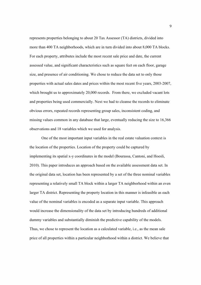
represents properties belonging to about 20 Tax Assessor (TA) districts, divided into

more than 400 TA neighborhoods, which are in turn divided into about 8,000 TA blocks.

For each property, attributes include the most recent sale price and date, the current

assessed value, and significant characteristics such as square feet on each floor, garage

size, and presence of air conditioning. We chose to reduce the data set to only those

properties with actual sales dates and prices within the most recent five years, 2003-2007,

which brought us to approximately 20,000 records. From there, we excluded vacant lots

and properties being used commercially. Next we had to cleanse the records to eliminate

obvious errors, repeated records representing group sales, inconsistent coding, and

missing values common in any database that large, eventually reducing the size to 16,366

observations and 18 variables which we used for analysis.

One of the most important input variables in the real estate valuation context is

the location of the properties. Location of the property could be captured by

implementing its spatial x-y coordinates in the model (Bourassa, Cantoni, and Hoesli,

2010). This paper introduces an approach based on the available assessment data set. In

the original data set, location has been represented by a set of the three nominal variables

representing a relatively small TA block within a larger TA neighborhood within an even

larger TA district. Representing the property location in this manner is infeasible as each

value of the nominal variables is encoded as a separate input variable. This approach

would increase the dimensionality of the data set by introducing hundreds of additional

dummy variables and substantially diminish the predictive capability of the models.

Thus, we chose to represent the location as a calculated variable, i.e., as the mean sale

price of all properties within a particular neighborhood within a district. We believe that

10

such an attribute and/or the median sale price would normally be available to property tax

assessors, appraisers, real estate agents, banks, home sellers, realtors, private professional

assessors as well as potential buyers. According to the information provided by the tax

assessment official in April 2009, one of the ways to assess (or reassess) the value of a

property for tax purposes in the area in which these data were collected, is to sum up the

sale prices of all similar properties sold recently in the immediate neighborhood of the

house, divide it by the total square footage of these sold properties and multiply by the

square footage of the property to be assessed.

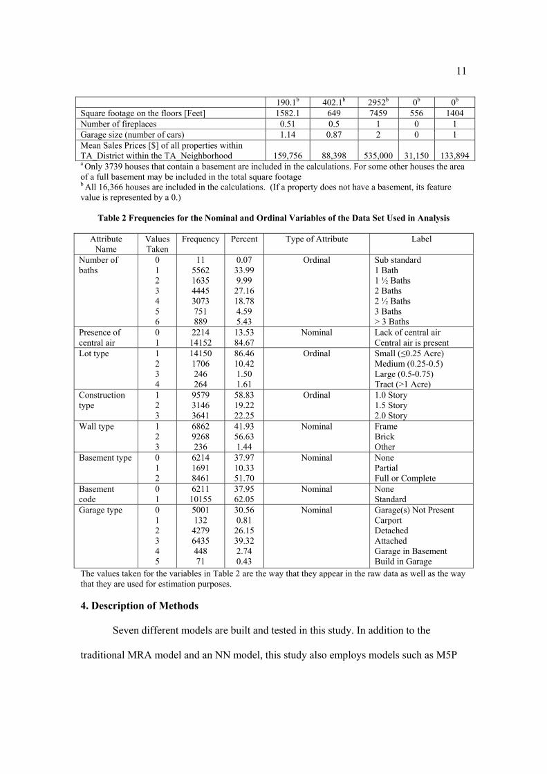
The basic descriptive statistics of this data set, including frequency counts and

percentages, are presented in Tables 1 and 2. Each variable in Table 1 (measured on the

ratio scale or interval scale) represents an input to the models in our study. In Table 2

each of the ordinal variables, Number of baths and Lot type, represents an input. For the

variable Construction type each level represents a dummy variable. As a result, 3 dummy

variables are created as input, one for each construction type level. For nominal variables

each distinct level of the variables is represented by a dummy variable in our models. For

example, since the Garage type variable has 6 levels (0-5), 6 dummy variables are created

as input to the models, one for each level. One can see that the data set we used for

analysis is very diverse in terms of neighborhoods, sale prices, lot types and sizes, year

built, square footage on the floors, number of bathrooms, etc.

Table 1 Descriptive Statistics for the Ratio and Interval Variables of the Data Set Used in Analysis

Attribute Name Mean Standard Deviation Max Min Median

Sale price [$] 159,756 98,686 865,000 17,150 134,925 Year property sold 2005 1.2 2007 2003 2006 Quarter of sale 2.48 1.04 4 1 2 Land size [Acres] 0.27 0.48 17.34 0.15 0.21 Year built 1968 31.2 2006 1864 1967 Square footage in the basement [Feet] 831.9a 416.7a 2952a 30a 753a

11

190.1b 402.1b 2952b 0b 0b Square footage on the floors [Feet] 1582.1 649 7459 556 1404 Number of fireplaces 0.51 0.5 1 0 1 Garage size (number of cars) 1.14 0.87 2 0 1 Mean Sales Prices [$] of all properties within TA_District within the TA_Neighborhood 159,756 88,398 535,000 31,150 133,894 a Only 3739 houses that contain a basement are included in the calculations. For some other houses the area of a full basement may be included in the total square footage b All 16,366 houses are included in the calculations. (If a property does not have a basement, its feature value is represented by a 0.)

Table 2 Frequencies for the Nominal and Ordinal Variables of the Data Set Used in Analysis

Attribute Name

Values Taken

Frequency Percent Type of Attribute Label

Number of baths

0 1 2 3 4 5 6

11 5562 1635 4445 3073 751 889

0.07 33.99 9.99 27.16 18.78 4.59 5.43

Ordinal Sub standard 1 Bath 1 ½ Baths 2 Baths 2 ½ Baths 3 Baths > 3 Baths

Presence of central air

0 1

2214 14152

13.53 84.67

Nominal Lack of central air Central air is present

Lot type 1 2 3 4

14150 1706 246 264

86.46 10.42 1.50 1.61

Ordinal Small (≤0.25 Acre) Medium (0.25-0.5) Large (0.5-0.75) Tract (>1 Acre)

Construction type

1 2 3

9579 3146 3641

58.83 19.22 22.25

Ordinal 1.0 Story 1.5 Story 2.0 Story

Wall type 1 2 3

6862 9268 236

41.93 56.63 1.44

Nominal Frame Brick Other

Basement type 0 1 2

6214 1691 8461

37.97 10.33 51.70

Nominal None Partial Full or Complete

Basement code

0 1

6211 10155

37.95 62.05

Nominal None Standard

Garage type 0 1 2 3 4 5

5001 132 4279 6435 448 71

30.56 0.81 26.15 39.32 2.74 0.43

Nominal Garage(s) Not Present Carport Detached Attached Garage in Basement Build in Garage

The values taken for the variables in Table 2 are the way that they appear in the raw data as well as the way that they are used for estimation purposes. 4. Description of Methods

Seven different models are built and tested in this study. In addition to the

traditional MRA model and an NN model, this study also employs models such as M5P

12

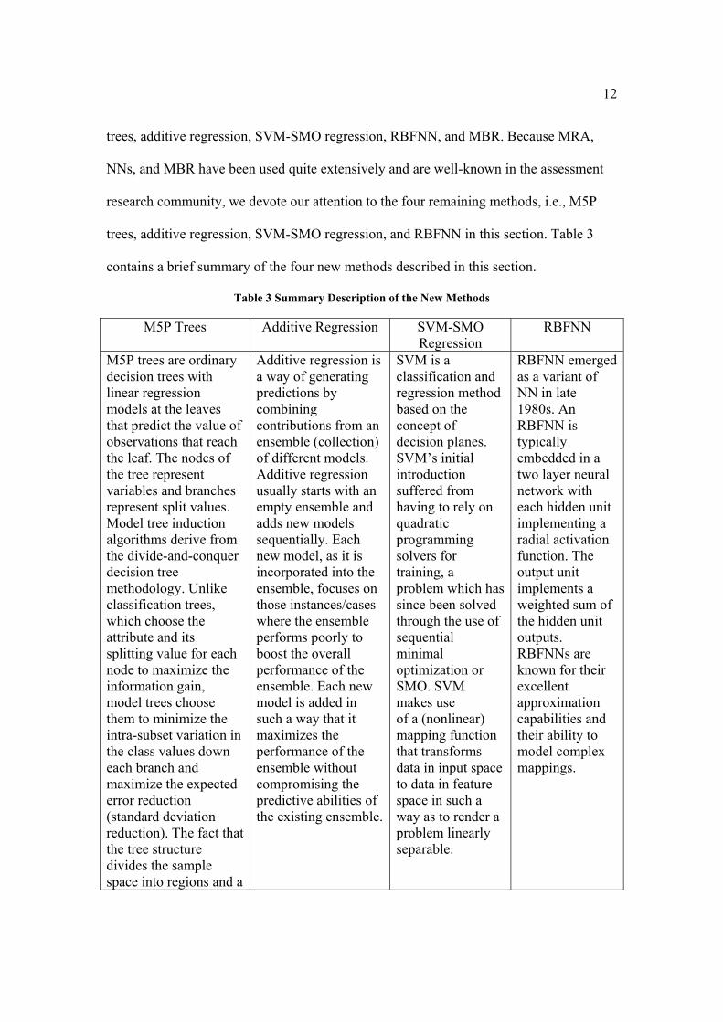
trees, additive regression, SVM-SMO regression, RBFNN, and MBR. Because MRA,

NNs, and MBR have been used quite extensively and are well-known in the assessment

research community, we devote our attention to the four remaining methods, i.e., M5P

trees, additive regression, SVM-SMO regression, and RBFNN in this section. Table 3

contains a brief summary of the four new methods described in this section.

Table 3 Summary Description of the New Methods

M5P Trees Additive Regression SVM-SMO Regression

RBFNN

M5P trees are ordinary decision trees with linear regression models at the leaves that predict the value of observations that reach the leaf. The nodes of the tree represent variables and branches represent split values. Model tree induction algorithms derive from the divide-and-conquer decision tree methodology. Unlike classification trees, which choose the attribute and its splitting value for each node to maximize the information gain, model trees choose them to minimize the intra-subset variation in the class values down each branch and maximize the expected error reduction (standard deviation reduction). The fact that the tree structure divides the sample space into regions and a

Additive regression is a way of generating predictions by combining contributions from an ensemble (collection) of different models. Additive regression usually starts with an empty ensemble and adds new models sequentially. Each new model, as it is incorporated into the ensemble, focuses on those instances/cases where the ensemble performs poorly to boost the overall performance of the ensemble. Each new model is added in such a way that it maximizes the performance of the ensemble without compromising the predictive abilities of the existing ensemble.

SVM is a classification and regression method based on the concept of decision planes. SVM’s initial introduction suffered from having to rely on quadratic programming solvers for training, a problem which has since been solved through the use of sequential minimal optimization or SMO. SVM makes use of a (nonlinear) mapping function that transforms data in input space to data in feature space in such a way as to render a problem linearly separable.

RBFNN emerged as a variant of NN in late 1980s. An RBFNN is typically embedded in a two layer neural network with each hidden unit implementing a radial activation function. The output unit implements a weighted sum of the hidden unit outputs. RBFNNs are known for their excellent approximation capabilities and their ability to model complex mappings.

13

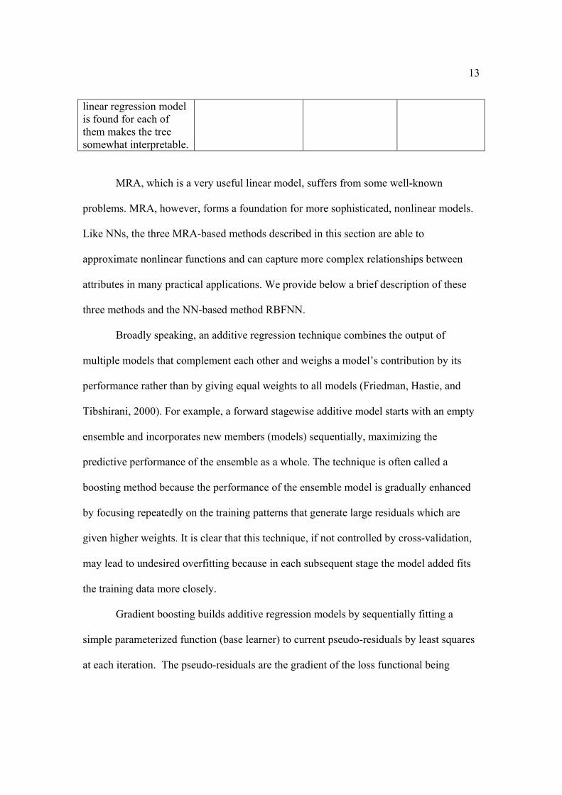
linear regression model is found for each of them makes the tree somewhat interpretable.

MRA, which is a very useful linear model, suffers from some well-known

problems. MRA, however, forms a foundation for more sophisticated, nonlinear models.

Like NNs, the three MRA-based methods described in this section are able to

approximate nonlinear functions and can capture more complex relationships between

attributes in many practical applications. We provide below a brief description of these

three methods and the NN-based method RBFNN.

Broadly speaking, an additive regression technique combines the output of

multiple models that complement each other and weighs a model’s contribution by its

performance rather than by giving equal weights to all models (Friedman, Hastie, and

Tibshirani, 2000). For example, a forward stagewise additive model starts with an empty

ensemble and incorporates new members (models) sequentially, maximizing the

predictive performance of the ensemble as a whole. The technique is often called a

boosting method because the performance of the ensemble model is gradually enhanced

by focusing repeatedly on the training patterns that generate large residuals which are

given higher weights. It is clear that this technique, if not controlled by cross-validation,

may lead to undesired overfitting because in each subsequent stage the model added fits

the training data more closely.

Gradient boosting builds additive regression models by sequentially fitting a

simple parameterized function (base learner) to current pseudo-residuals by least squares

at each iteration. The pseudo-residuals are the gradient of the loss functional being

14

minimized, with respect to the model values at each training data point, evaluated at the

current step. More formally the boosting technique can be presented as follows

(Friedman, Hastie, and Tibshirani, 2000). Let y and },....,{ 1 nxx=x represent an output

variable and input variables, respectively. Given a training sample Niiy 1},{ x of known

),( xy -values, the goal is to find a function )(* xF that maps x to ,y such that over the joint

distribution of all ),( xy -values, the expected value of some specified loss function

))(,( xΨ Fy is minimized:

)).(,(min arg)( ,)(

* xΨx xxFyEF yF

= (1)

Boosting approximates )(* xF by an additive expansion of the form

∑=

=M

mmmhF

0),;()( axx β (2)

where the functions );( axh (base learner) are usually chosen to be simple functions of

x with parameters }.,....,{ 21 maaa=a The expansion coefficients Mm 0}{β and the parameters

Mm 0}{a are jointly fit to the training data in a forward stage-wise manner. The method

starts with an initial guess ),(0 xF and then for Mm ,....,2,1=

));()(,(minarg),(

11, ∑

=− +=

N

iiimimm hFy axxΨa

aββ

β (3)

and

).;()()( 1 mmmm hFF axxx β+= − (4)

15

Gradient boosting by Friedman et al. (2000) approximately solves (3) for arbitrary

(differentiable) loss function ))(,( xΨ Fy with a two step procedure. First, the function

);( axh is fit by least-squares

∑=

−=N

iiimm hy

1,)];(~[minarg 2

aaxa ρ

ρ (5)

to the current pseudo-residuals

)()()(

))(,(~xx 1m

xx

−=

⎥⎦

⎤⎢⎣

⎡∂

Ψ∂−=

FFi

iiim F

Fyy (6)

Then, given ),;( mh ax the optimal value of the coefficient mβ is determined

)).;()(,(minarg 1

1miimi

N

im hFy axxΨ ββ

β+= −

=∑ (7)

This strategy replaces a potentially difficult function optimization problem (3) by one

based on least-squares (5), followed by a single parameter optimization (7) based on the

general loss criterion .Ψ (adapted from Friedman et al. (2000)).

M5P tree, or M5 model tree, is a predictive technique that has become

increasingly noticed since Quinlan introduced it in 1992 (Quinlan, 1992; Wang and

Witten, 1997). Model trees are ordinary decision trees with linear regression models at

the leaves that predict the value of observations that reach the leaf. The nodes of the tree

represent variables and branches represent split values. The fact that the tree structure

divides the sample space into regions and a linear regression model is found for each of

them makes the tree somewhat interpretable. Model tree induction algorithms derive from

the divide-and-conquer decision tree methodology. Unlike classification trees, which

choose the attribute and its splitting value for each node to maximize the information

16

gain, model trees minimize the intra-subset variation in the class values down each

branch. In other words, for each node a model tree chooses an attribute and its splitting

value to maximize the expected error reduction (standard deviation reduction).

An M5P tree is built in three stages (Wang and Witten, 1997). In the first stage a

decision tree induction algorithm is used to build an initial tree. Let T represent a set of

training cases where each training case consists of a set of attributes and an associated

target value. A divide and conquer method is used to split T into subsets based on the

outcomes of testing. This method is then applied to the resulting subsets recursively. The

splitting criterion is based on the standard deviation of the subset of values that reach the

current node as an error measure. Each attribute is then tested by calculating its expected

error reduction at the node. The attribute that maximizes the error reduction is chosen.

The standard deviation reduction is calculated as follows:

)()( i

i

i TsdTTTsdSDR ×−= ∑ (8)

where T is the set of training cases and Ti are the subsets that result from splitting the

cases that reach the node according to the chosen attribute. Splitting in M5P stops when

either there is very little variation in the values of the cases that reach a node or only a

very few cases remain.

In the second stage of the tree construction process the tree is pruned back from

each leaf. The defining characteristic of an M5P tree is in replacing a node being pruned

by a regression model instead of a constant target value. In the pruning process the

average of the absolute differences between the target value and actual value of all the

cases reaching a node to be pruned is calculated as an estimate for the expected error.

17

This average will underestimate the expected error because of the unseen cases so it is

multiplied by the factor

)()(

vnvnp

−+

=′ (9)

where n is the number of training cases that reach the node and v is the number of

parameters in the model that represents the class value at that node.

The last stage is called smoothing to remove any sharp discontinuities that exist

between neighboring leaves of the pruned tree. The smoothing calculation is given as

follows:

knkgnpp

++

=′ (10)

where p’ is the predicted value passed up to the next higher node, p is the predicted value

passed to this node from below, q is the predicted value of the model at this node, n is the

number of training cases that reach the node below, and k is a constant (the common

value is 15). The above described process of building a model tree by Quinlan (1992) is

improved by Wang and Witten (1997) and this study uses the improved version referred

to as M5’ or M5P.

SVM is a relatively new machine learning technique originally developed by

Vapnik (1998). The basic concept behind SVM is to solve a problem, i.e., classification

or regression, without having to solve a more difficult problem as an intermediate step.

SVM does that by mapping the non-linear input attribute space into a high dimensional

feature space. A linear model constructed in the new feature space represents a non-linear

classifier in the original attribute space. This linear model in the feature space is called

18

the maximum margin hyperplane, which provides maximum separation into decision

classes in the original attribute space. The training cases closest to the maximum margin

hyperplane are called support vectors.

As an example suppose we have data from an input/attribute space x with an

unknown distribution P(x,y), where y is binary, i.e., y can have one of two values. This

two-class case can be extended to a k class classification case by constructing k two-class

classifiers (Vapnik, 1998). In SVM a hyperplane separating the binary decision classes

can be represented by the following equation:

0wy +⋅= xw (11)

where y is the output, x is the input vector, and w is the weight vector. The maximum

margin hyperplane can be represented as follows (Cui and Curry, 2005):

∑ ⋅+= xx )(iyaby ii (12)

where yi is the output for the training case x(i), b and ai are parameters to be determined

by the training algorithm, and x is the test case. Note that x(i) and x are vectors and x(i)

are the support vectors. Though the example given above is for the binary classification

case, generalization to multiclass classification is possible. For an m class case, a simple

and effective procedure is to train one-versus-rest binary classifiers (say, “one” positive,

“rest” negative) and assign a test observation to the class with the largest positive

distance (Boser, Guyon, and Vapnik, 1992; Vapnik, 1998). This procedure has been

shown to give excellent results (Cui and Curry, 2005).

The above discussion has been restricted to the classification cases. A

generalization to regression estimation is also possible. In the case of regression

19

estimation we have Ry∈ and we are trying to construct a linear function in the feature

space so that the training cases stay within an error > 0. This can be written as a quadratic

programming problem in terms of kernels:

)),((∑+= xx iKyaby ii (13)

where )),(( xx iK is a kernel function (see next paragraph).

Vapnik (1998) shows that, for linearly separable data, the SVM can find the

unique and optimal classifier called the maximum margin classifier or optimal margin

classifier. In practice, however, the data or observations are rarely linearly separable in

the original attribute space, but may be linearly separable in a higher dimensional space

specially constructed through mapping. SVM uses a kernel-induced transformation to

map the attribute space into the higher dimensional feature space. SVM then finds an

optimal linear boundary in the feature space that maps to the nonlinearly separable data in

the original attribute space. Converting to the feature space may be time consuming and

the result difficult to store if the feature space is high in dimensions. The kernel function

allows one to construct a separating hyperplane in the higher dimensional feature space

without explicitly performing the calculations in the feature space. Popular kernel

functions include the polynomial kernel

dxyyxK )1(),( += (14)

and the Gaussian radial basis function

))(1exp(),( 2

2 yxyxK −−

=δ

(15)

20

where d is the degree of the polynomial kernel and is the bandwidth of the Gaussian

radial basis function kernel.

Since its introduction SVM has attracted intense interest because of its admirable

qualities, but it had been hindered for years by the fact that quadratic programming

solvers had been the only training algorithm. Osuna et al. (1997) shows that SVMs can be

optimized by decomposing a large quadratic programming problem into a series of

smaller quadratic programming. Platt (1998) introduced sequential minimal optimization

as a new optimization algorithm. Because SMO uses a subproblem of size two, each

subproblem has an analytical solution. Thus, for the first time, SVMs could be optimized

without a QP solver.

An RBFNN differs from a multilayer perceptron (a feed-forward NN with back-

propagation) in the way the hidden neurons perform computations (Park and Sandberg,

1991; Poggio and Girosi, 1990). Each neuron represents a point in input space, and its

output for a given training case depends on the distance between its point and the target

of the training. The closer these two points are, the stronger the activation. The RFBNN

uses nonlinear bell-shaped Gaussian activation functions whose width may be different

for each neuron. The RBFs are embedded in a two layer network. The Gaussian

activation function for RBFNN is given by:

⎥⎦

⎥⎢⎣

⎢−−−= ∑

−1

)()(exp)(j

jT

j μXμXXφ (16)

for j=1,…,L , where X is the input feature vector and L is the number of neurons in the

hidden layer. jμ and ∑ j are the mean and covariance matrix of the jth Gaussian

function. The output layer forms a linear combination from the outputs of neurons in the

21

hidden layer which are fed to the sigmoid function. The output layer implements a

weighted sum of the hidden-layer outputs:

∑= )()( XX jjkk ϕλψ (17)

for k=1,…,M , where jkλ are the output weights, each represents a connection between a

hidden layer unit and an output unit and M represents the number of units in the output

layer. For application in mass assessment M will be 1. jkλ shows the contribution of a

hidden unit to the corresponding output unit. When 0>jkλ , the activation of the hidden

unit j is contained in the activation of the output field k. The output of the radial basis

function is limited to the interval (0,1) by the sigmoidal function as follows:

[ ])(exp11)(

XX

kkY

ψ−+= (18)

for k=1,…,M .

The network learns two sets of parameters: the centers and width of the Gaussian

functions by employing clustering and the weights used to form the linear combination of

the outputs obtained from the hidden layer. As the first set of parameters can be obtained

independently of the second set, RFBNN learns almost instantly if the number of hidden

units is much smaller than the number of training patterns. Unlike multilayer perceptron,

the RBFNN, however, cannot learn to ignore irrelevant attributes because it gives them

the same weight in distance computations (adapted from Bors (2001)).

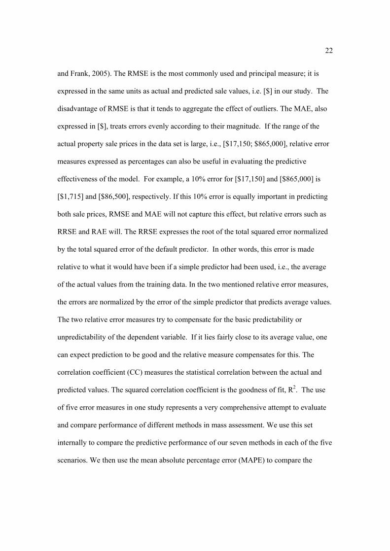
5. Error Measures and Performance Criteria

Model performance measures are essential in evaluating the predictive accuracy

of the models. Table 4 presents the error measures used for numeric prediction (Witten

22

and Frank, 2005). The RMSE is the most commonly used and principal measure; it is

expressed in the same units as actual and predicted sale values, i.e. [$] in our study. The

disadvantage of RMSE is that it tends to aggregate the effect of outliers. The MAE, also

expressed in [$], treats errors evenly according to their magnitude. If the range of the

actual property sale prices in the data set is large, i.e., [$17,150; $865,000], relative error

measures expressed as percentages can also be useful in evaluating the predictive

effectiveness of the model. For example, a 10% error for [$17,150] and [$865,000] is

[$1,715] and [$86,500], respectively. If this 10% error is equally important in predicting

both sale prices, RMSE and MAE will not capture this effect, but relative errors such as

RRSE and RAE will. The RRSE expresses the root of the total squared error normalized

by the total squared error of the default predictor. In other words, this error is made

relative to what it would have been if a simple predictor had been used, i.e., the average

of the actual values from the training data. In the two mentioned relative error measures,

the errors are normalized by the error of the simple predictor that predicts average values.

The two relative error measures try to compensate for the basic predictability or

unpredictability of the dependent variable. If it lies fairly close to its average value, one

can expect prediction to be good and the relative measure compensates for this. The

correlation coefficient (CC) measures the statistical correlation between the actual and

predicted values. The squared correlation coefficient is the goodness of fit, R2. The use

of five error measures in one study represents a very comprehensive attempt to evaluate

and compare performance of different methods in mass assessment. We use this set

internally to compare the predictive performance of our seven methods in each of the five

scenarios. We then use the mean absolute percentage error (MAPE) to compare the

23

predictive accuracy of our best models to the Freddie Mac criterion, explained below in

the section on computer simulation results.

Table 4 Performance measures for numeric prediction. Legend: pi – predicted sale price, ai – actual sale price, n – number of observations, i=1…n

Error/Performance Measure Formula Root Mean-squared Error (RMSE)

n

apn

iii∑

=

−1

2)(

Mean Absolute Error (MAE)

n

apn

iii∑

=

−1

||

Root Relative Squared Error (RRSE)

n

aa

aa

apn

ii

n

ii

n

iii ∑

∑

∑=

=

= =−

−1

1

2

1

2

where,)(

)(

Relative Absolute Error (RAE)

∑

∑

=

=

−

−

n

ii

n

iii

aa

ap

1

1

||

||

Correlation Coefficient (CC) Goodness of Fit (R2) = CC2

n

pp

n

aaS

n

ppS

n

aappS

SSS

n

iii

A

i

p

n

iii

PAap

PA

∑∑∑

∑

=

=

=−

−=

−

−=

−

−−=

1

22

1

and,1

)(,

1

)(

,1

))((where,

Mean Absolute Percentage Error (MAPE)

na

apn

i i

ii∑=

−

1

6. Computer Simulation Scenarios

The simulations were performed with SAS Enterprise Miner (EM) and Weka

(Witten and Frank, 2005). The former is a well-known data analysis software developed

and maintained by the SAS company (www.sas.com) and the latter is an open source

software product designed for data mining available from the University of Waikato,

24

New Zealand (Witten and Frank, 2005). Each of these software products is equipped with

a set of convenient tools for modeling. We performed computer simulation under five

different scenarios and measured the predictive effectiveness of the methods on the test

set by five performance measures: MAE, RMSE, RRSE, RAE, and R2. In scenarios 1 and

2 we tested the models on the entire data set that contained very heterogeneous properties

in terms of their sale prices and features. Tables 1 and 2 show the descriptive statistics,

including frequencies of the features used. For example, the smallest and largest property

sale prices are [$17,150] and [$865,000], respectively.

In scenario 1 we used the 16 original input variables (along with the dummy

variables), whereas in scenario 2, in addition to the original 16 input variables (also with

dummy variables), we used an additional calculated input variable to represent

“location”. This variable is introduced to capture the location dimension and is defined as

the mean sale price of the properties within the tax assessment (TA) district within the

TA neighborhood, which, depending on the neighborhood, contains between 10 and 50

properties. Adding “location” as an input, as any assessor would do, significantly lowered

the error estimates, as shown later in the paper. This need to cluster or segment the data

set can minimize problems associated with heteroscedasticity (Mark and Goldberg, 1988;

Newsome and Zietz, 1992). Newsome and Zietz (1992) suggest that location based on

home prices can be used as a basis for segmentation.

Since any given house may sell for a different price in a later year than it would in

a previous year, even with no change in its attributes, sale prices have to be adjusted for

general market inflation/deflation. Since the 16,366 records represent houses sold

between 2003 and 2007, in this study we used the Year of sale and Quarter of sale

25

variables to capture the general market macroeconomic effect in scenarios 1-4. As both

variables are measured on the interval scale, we treated them as numeric variables and

they represent two inputs to the models. In scenario 5, we calculated the Age of the

properties from the Year of sale, Quarter of sale and Year built to capture the general

market effect. The Age variable, which is clearly on the ratio scale, replaced the three

mentioned variables in the models. The market effect could also be handled by a

technique used in Guan, Zurada, and Levitan (2008). In that technique the sale prices in

the data set had been market-adjusted before they were used in the models. Another

alternative would be to limit the sample to sales in a single year. But that itself would

limit the validity and generalizability of the results due to the smaller data set size. It

could be argued that the market-adjusted technique or just using the Age of the properties

variable may have more merit as it reduces the number of input variables in the models

and can make models simpler to explain.

In scenarios 3 through 5, we used automatic K-means clustering to group the

properties into several more homogeneous clusters. K-means is one of the popular

clustering procedures used to find homogeneous clusters in a heterogeneous data set. It

works well with large data sets, and as most clustering algorithms, it is quite sensitive to

the distance measures. The k-means algorithm may not work too well with overlapping

clusters and may be sensitive to the selection of initial seeds, i.e., embryonic clusters. We

applied the Euclidean distance to measure the similarity between observations and ran the

procedure for different initial seeds making sure that these produce similar clusters. We

tested the models on each cluster, and analyzed the models’ performance measures.

Grouping properties into clusters allowed us to find out that the models tested on

26

segments containing more expensive and more recently built properties yielded better

overall predictive performance, i.e., they produced significantly lower error estimates

than models built on clusters consisting of mid-range and low-end properties.

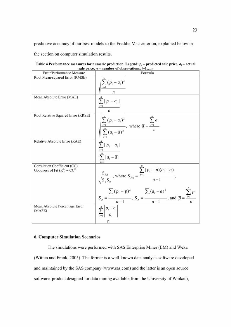
In scenario 3 we built clusters based on all the normalized 17 input variables,

including “location”, and the normalized output variable, the property sale price. Table 5

presents the features of the properties for the three clusters created. For example, one can

see that cluster 1 includes 4,792 transactions representing more affluent properties with

the mean sale price of [$269,388] and larger properties with the average floor size of

2,261 sq. ft. as well as more recently built properties with the mean Year built=1993.

Clusters 2 and 3 represent less expensive properties which are 50-60 years old.

Table 5 Feature Means and Standard Deviations for Three Clusters built in Scenario 3

Number of

Obser-vations

Sale price [$]

Location [$]

Square footage on

floors

Year built

Number of

baths

Fire Place

Land size

Garage Size

Cluster 1 4792 269,388 94,593

256,852 80,167

2,261 621

1993 18

4.2 1.1

0.93 0.25

0.35 0.57

1.8 0.4

Cluster 2 4836 133,784 59,264

131,110 55,881

1,364 400

1955 25

2.2 1.2

0.5 0.5

0.24 0.41

1.1 0.8

Cluster 3 6738 100,426 47,109

111,261 50,231

1,256 407

1960 32

1.9 1.1

0.24 0.43

0.23 0.45

0.7 0.8

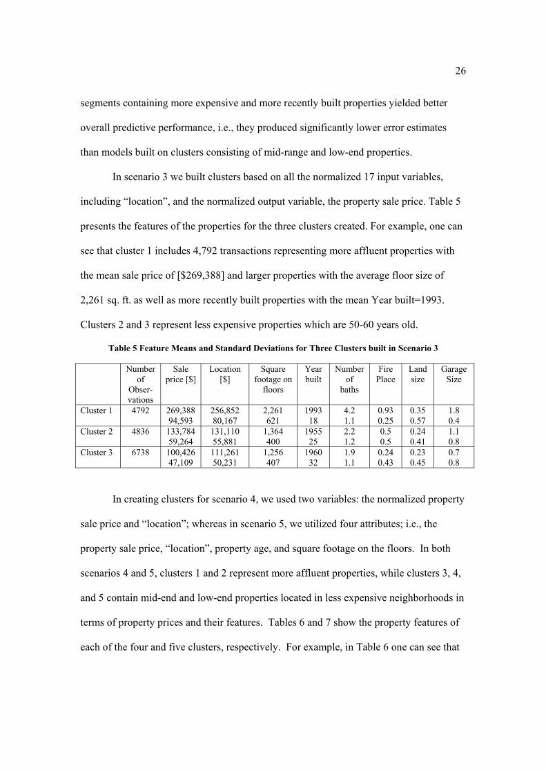
In creating clusters for scenario 4, we used two variables: the normalized property

sale price and “location”; whereas in scenario 5, we utilized four attributes; i.e., the

property sale price, “location”, property age, and square footage on the floors. In both

scenarios 4 and 5, clusters 1 and 2 represent more affluent properties, while clusters 3, 4,

and 5 contain mid-end and low-end properties located in less expensive neighborhoods in

terms of property prices and their features. Tables 6 and 7 show the property features of

each of the four and five clusters, respectively. For example, in Table 6 one can see that

27

cluster 1 includes 3,188 more affluent properties located in more affluent neighborhoods

with the mean sale price of [$318,399]; larger properties in terms of the floor size (mean

= 2,510 sq. ft.) as well as more recently built properties with the mean Year built=1992.

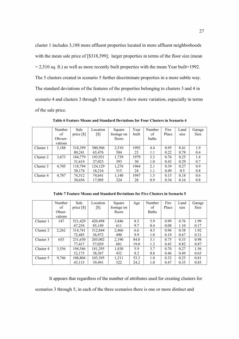
The 5 clusters created in scenario 5 further discriminate properties in a more subtle way.

The standard deviations of the features of the properties belonging to clusters 3 and 4 in

scenario 4 and clusters 3 through 5 in scenario 5 show more variation, especially in terms

of the sale price.

Table 6 Feature Means and Standard Deviations for Four Clusters in Scenario 4

Number of

Obvser-vations

Sale price [$]

Location [$]

Square footage on

floors

Year built

Number of

baths

Fire Place

Land size

Garage Size

Cluster 1 3,188 318,399 80,241

300,506 65,476

2,510 584

1992 23

4.4 1.1

0.95 0.22

0.41 0.78

1.9 0.4

Cluster 2 3,673 184,779 31,614

193,931 27,023

1,739 393

1979 30

3.3 1.0

0.76 0.43

0.25 0.29

1.4 0.7

Cluster 3 4,705 118,794 30,174

124,129 18,216

1,276 315

1964 24

2.1 1.1

0.39 0.49

0.27 0.5

0.9 0.8

Cluster 4 4,787 74,512 30,656

74,641 17,905

1,140 324

1947 28

1.5 0.9

0.15 0.34

0.18 0.16

0.6 0.8

Table 7 Feature Means and Standard Deviations for Five Clusters in Scenario 5

Number of

Obser-vations

Sale price [$]

Location [$]

Square footage on

floors

Age Number of

Baths

Fire Place

Land size

Garage Size

Cluster 1 147 521,429 67,254

420,498 85,149

3,846 611

8.5 9.7

5.9 0.4

0.99 0.08

0.76 1.10

1.99 0.17

Cluster 2 2,262 314,741 72,485

312,844 36,972

2,466 490

6.6 9.9

4.5 1.0

0.96 0.19

0.38 0.67

1.92 0.31

Cluster 3 655 231,630 77,417

205,002 57,029

2,190 681

84.0 19.0

3.1 1.3

0.75 0.43

0.33 0.82

0.98 0.87

Cluster 4 3,556 194,546 52,175

181,295 38,367

1,830 432

5.9 8.2

3.7 0.8

0.70 0.46

0.27 0.49

1.56 0.63

Cluster 5 9,746 108,804 43,115

103,395 39,491

1,211 322

53.3 24.2

1.8 1.0

0.32 0.47

0.23 0.35

0.81 0.85

It appears that regardless of the number of attributes used for creating clusters for

scenarios 3 through 5, in each of the three scenarios there is one or more distinct and

28

homogeneous cluster that contains higher-end properties and other more heterogeneous

and mixed clusters that include mid-range and less expensive properties. The means and

standard deviations of the features presented in Tables 6 and 7 across all clusters confirm

these observations. For example, in cluster l of scenario 5 (Table 7), the percentage of

the standard deviation of the actual sale prices to the mean of actual sale prices is

[$67,254]/[$521,429]=12.9% and the same ratio for cluster 5 is

[$43,115]/[$108,804]=39.6%.

In all five scenarios, we used 10-fold cross-validation and repeated the

experiments from 3 to 10 times to obtain true, unbiased and reliable error measures of the

models. In 10-fold cross-validation, a data set is first randomized and then divided into 10

folds (subsets), where each of the 10 folds contains approximately the same number of

observations (sales records). First, folds 1-9 of the data set are used for building a model

and fold 10 alone is used for testing the model. Then, folds 1-8, and 10 are employed for

training a model and fold 9 alone is used for testing, and so on. A 10-fold cross-validation

provides 10 error estimates. For clusters containing a larger number of observations, for

example >5,000, we repeated the 10-fold cross-validation experiment 3 times, and for

clusters with a smaller number of observations we repeated it 10 times. In each new

experiment the data set was randomized again. This way, we obtained either 30 or 100

unbiased, reliable, and realistic error estimates. This approach also ensures that data

subsets used to train the models are completely independent from data subsets used to test

the models. The number of folds, 10, and the number of experiments, i.e., 3 or 10, have

been shown to be sufficient to achieve stabilization of cumulative average error

measures.

29

We averaged the error estimates across all folds and runs and ensured that training

samples we used to build models were fully independent of the test samples. The

statistical significance among the performance of the seven models was measured by a

paired two-tailed t-test at α=0.05 (Witten and Frank, 2005) to see if the error measures

across the models within each scenario were significantly different from the MRA

models, which were the reference points.

7. Results from Computer Simulations

The simulation results showed that nontraditional regression methods such as

additive regression, M5P trees, and SVM-SMO consistently outperformed MRA and

MBR in most simulation scenarios. However, in scenarios 1 and 5, NN also performed

very well yielding significantly lower error estimates than MRA (Tables 8 and 12). In

scenario 1 MBR outperformed MRA (see Table 8). It appears that the AI-based methods

tend to perform better for heterogeneous data sets containing properties with mixed

features and the nontraditional regression methods produce better results for more

homogeneous clusters of properties.

Analysis of each of the five simulation scenarios and clusters allows one to gain more

insight into the performance of the models. In scenario 1 (Table 8), which includes all

properties with very mixed features, additive regression, M5P trees, NNs, RBFNN, and

MBR significantly outperform MRA across most error measures. However, there is no

significant difference between the performance of MRA and SVM-SMO.

In scenario 2, additive regression and M5P tree outperform MRA across all five error

measures (Table 9). However, there is no significant difference between NN, and SVM-

SMO compared to MRA. The RBFNN’s and MBR’s performances are significantly

30

worse than that of MRA. One can also see that the models created on all samples using

an additional attribute “location” generate significantly lower error estimates (Table 9)

than those in scenario 1 (Table 8).

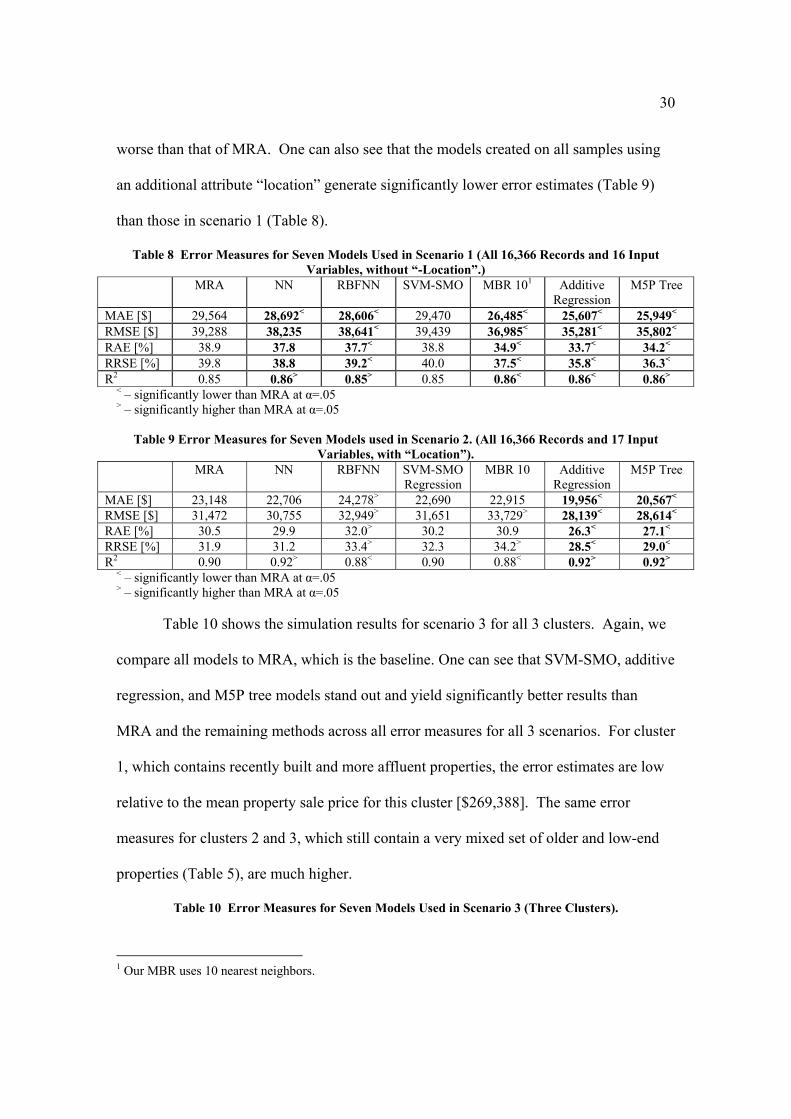
Table 8 Error Measures for Seven Models Used in Scenario 1 (All 16,366 Records and 16 Input Variables, without “-Location”.)

MRA NN RBFNN

SVM-SMO MBR 101 Additive Regression

M5P Tree

MAE [$] 29,564 28,692< 28,606< 29,470 26,485< 25,607< 25,949< RMSE [$] 39,288 38,235 38,641< 39,439 36,985< 35,281< 35,802< RAE [%] 38.9 37.8 37.7< 38.8 34.9< 33.7< 34.2< RRSE [%] 39.8 38.8 39.2< 40.0 37.5< 35.8< 36.3< R2 0.85 0.86> 0.85> 0.85 0.86< 0.86< 0.86>

< – significantly lower than MRA at α=.05 > – significantly higher than MRA at α=.05

Table 9 Error Measures for Seven Models used in Scenario 2. (All 16,366 Records and 17 Input Variables, with “Location”).

MRA NN RBFNN SVM-SMORegression

MBR 10 Additive Regression

M5P Tree

MAE [$] 23,148 22,706 24,278> 22,690 22,915 19,956< 20,567< RMSE [$] 31,472 30,755 32,949> 31,651 33,729> 28,139< 28,614< RAE [%] 30.5 29.9 32.0> 30.2 30.9 26.3< 27.1< RRSE [%] 31.9 31.2 33.4> 32.3 34.2> 28.5< 29.0< R2 0.90 0.92> 0.88< 0.90 0.88< 0.92> 0.92>

< – significantly lower than MRA at α=.05 > – significantly higher than MRA at α=.05

Table 10 shows the simulation results for scenario 3 for all 3 clusters. Again, we

compare all models to MRA, which is the baseline. One can see that SVM-SMO, additive

regression, and M5P tree models stand out and yield significantly better results than

MRA and the remaining methods across all error measures for all 3 scenarios. For cluster

1, which contains recently built and more affluent properties, the error estimates are low

relative to the mean property sale price for this cluster [$269,388]. The same error

measures for clusters 2 and 3, which still contain a very mixed set of older and low-end

properties (Table 5), are much higher.

Table 10 Error Measures for Seven Models Used in Scenario 3 (Three Clusters).

1 Our MBR uses 10 nearest neighbors.

31

MRA NN RBFNN SVM-SMO

Regression

MBR 10 Additive Regression

M5P Tree

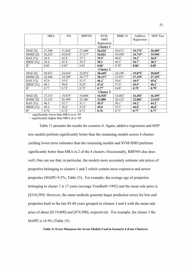
Cluster 1 MAE [$] 27,368 31,824> 27,640> 26,626< 29,671> 25,374< 26,685< RMSE [$] 36,235 43,010> 37,317> 36,022 43,950> 34,719< 35,996< RAE [%] 36.9 42.8> 37.3 35.9< 40.0> 34.2< 36.0< RRSE [%] 38.4 45.4> 39.5> 38.1 46.5> 36.7< 38.1< R2 0.85 0.83< 0.85 0.86> 0.79< 0.86> 0.85 Cluster 2 MAE [$] 20,833 24,824> 22,832> 20,449< 24,190> 19,875< 20,045< RMSE [$] 28,460 34,389> 30,777> 28,137< 33,951> 27,155< 27,255< RAE [%] 47.0 55.8> 51.5> 46.1< 54,6> 44.9< 45.6< RRSE [%] 48.1 58.0> 52.0> 47.6< 57.4> 45.9< 46.1< R2 0.77 0.72< 0.72< 0.77> 0.69< 0.79> 0.79> Cluster 3MAE [$] 17,133 19,419> 18,848> 16,928< 18,462> 16,303< 16,295< RMSE [$] 23,152 26,589> 25,386> 23,080 26,125> 22,002< 22,035< RAE [%] 46.5 52.7> 51.1> 45.9< 50.1> 44.2< 44.2< RRSE [%] 49.2 56.4> 53.9> 49.0 55.5> 46.8< 46.8< R2 0.76 0.72< 0.71< 0.76 0.71< 0.77> 0.77>

< – significantly lower than MRA at α=.05 > - significantly higher than MRA at α=.05

Table 11 presents the results for scenario 4. Again, additive regression and M5P

tree models perform significantly better than the remaining models across 4 clusters

yielding lower error estimates than the remaining models and SVM-SMO performs

significantly better than MRA in 2 of the 4 clusters. Occasionally, RBFNN also does

well. One can see that, in particular, the models more accurately estimate sale prices of

properties belonging to clusters 1 and 2 which contain more expensive and newer

properties (MAPE=9.5%, Table 15). For example, the average age of properties

belonging to cluster 1 is 17 years (average YearBuilt=1992) and the mean sale price is

[$318,399]. However, the same methods generate larger prediction errors for low-end

properties built in the last 45-60 years grouped in clusters 3 and 4 with the mean sale

price of about [$119,000] and [$74,500], respectively. For example, for cluster 3 the

MAPE is 16.9% (Table 15).

Table 11 Error Measures for Seven Models Used in Scenario 4 (Four Clusters).

32

MRA NN RBFNN SVM-SMO

Regression

MBR 10 Additive Regression

M5P Tree

Cluster 1 MAE [$] 31,579 33,259 29,887< 31,373< 32,196 29,187< 29,284< RMSE [$] 40,871 44,075 39,069< 41,004 46,529> 38,966< 38,970<

RAE [%] 50.7 53.3 47.9< 50.3< 51.6 46.8< 47.0< RRSE [%] 50.9 54.8 48.7 51.1 57.9> 48.5 48.5 R2 0.74 0.64 0.76> 0.74 0.67< 0.76> 0.76> Cluster 2 MAE [$] 17,832 18,828> 18,039 17,757 18,510 16,448< 16,978< RMSE [$] 23,003 24,897> 23,173 22,967 24,979> 21,709< 22,280< RAE [%] 69.1 72.9> 69.9 68.8 71.6 63.7< 65.8< RRSE [%] 72.9 78.9> 73.4 72.8 79.1> 68.8< 70.6< R2 0.48 0.48 0.46 0.48 0.42< 0.53> 0.50> Cluster 3MAE [$] 16,583 18,879> 16,696 16,341< 17,822> 15,969< 16,033< RMSE [$] 22,652 24,869> 22,786 22,659 24,670> 21,820< 21,906< RAE [%] 70.9 80.8> 71.4 69.9< 76.3> 68.3< 68.6< RRSE [%] 75.1 82.5> 75.5 75.1 81.8> 72.3< 72.6< R2 0.44 0.45 0.42 0.44 0.38< 0.48> 0.48> Cluster 4MAE [$] 16,545 19,073> 16,738> 16,392< 18,535> 16,282< 16,344< RMSE [$] 21,176 24,564> 21,403> 21,026< 24,646> 20,854< 20,937< RAE [%] 66.9 77.1> 67.8> 66.3< 75.0> 65.8< 66.1< RRSE [%] 69.1 80.1 > 69.8> 68.6< 80.4> 68.0< 68.3< R2 0.52 0.48< 0.52< 0.53> 0.41< 0.53> 0.53>

< – significantly lower than MRA at α=.05 > - significantly higher than MRA at α=.05

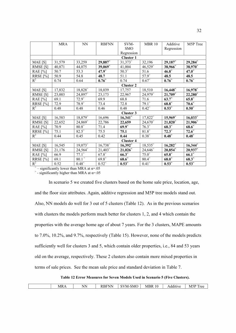
In scenario 5 we created five clusters based on the home sale price, location, age,

and the floor size attributes. Again, additive regression and M5P tree models stand out.

Also, NN models do well for 3 out of 5 clusters (Table 12). As in the previous scenarios

with clusters the models perform much better for clusters 1, 2, and 4 which contain the

properties with the average home age of about 7 years. For the 3 clusters, MAPE amounts

to 7.0%, 10.2%, and 9.7%, respectively (Table 15). However, none of the models predicts

sufficiently well for clusters 3 and 5, which contain older properties, i.e., 84 and 53 years

old on the average, respectively. These 2 clusters also contain more mixed properties in

terms of sale prices. See the mean sale price and standard deviation in Table 7.

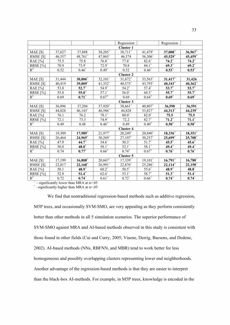
Table 12 Error Measures for Seven Models Used in Scenario 5 (Five Clusters).

MRA NN RBFNN SVM-SMO MBR 10 Additive M5P Tree

33

Regression Regression Cluster 1 MAE [$] 37,627 37,888 38,285> 38,711> 41,479> 37,008< 36,967< RMSE [$] 46,557 48,761> 47,865> 46,574 56,306> 45,529< 45,459< RAE [%] 75.5 75.8 76.8> 77.8> 82.6> 74.2< 74.2< RRSE [%] 70.9 73.9> 72.9> 70.8 84.1> 69.3< 69.2< R2 0.52 0.46< 0.49< 0.52 0.46< 0.53> 0.53> Cluster 2 MAE [$] 31,444 30,806< 32,101> 31,672> 33,563> 31,417< 31,426 RMSE [$] 40,419 39,809< 41,352> 40,575> 43,793> 40,343< 40,362< RAE [%] 53.8 52.7< 54.9> 54.2> 57.4> 53.7< 53.7< RRSE [%] 55.8 55.0< 57.1> 56.0> 60.5> 55.7< 55.7< R2 0.69 0.71> 0.67< 0.69 0.64< 0.69> 0.69> Cluster 3MAE [$] 36,896 37,204 37,920> 38,661> 40,807> 36,598 36,591 RMSE [$] 44,828 46,143> 46,586> 44,828 53,827> 44,313< 44,239< RAE [%] 76.1 76.2 78.1> 80.0> 82.0> 75.5 75.5 RRSE [%] 72.1 73.3 74.9> 72.2 82.7> 71.2< 71.1< R2 0.49 0.48 0.46< 0.49 0.40< 0.50> 0.50> Cluster 4MAE [$] 19,309 17,989< 21,977> 20,249> 20,840> 18,336< 18,351< RMSE [$] 26,464 24,965< 30,269> 27,107> 30,257> 25,699< 25,708< RAE [%] 47.9 44.7< 54.6> 50.3> 51.7> 45.5< 45.6< RRSE [%] 50.8 48.0< 58.1> 52.1> 58.1> 49.4< 49.4< R2 0.74 0.77> 0.66< 0.74< 0.67< 0.76> 0.76> Cluster 5 MAE [$] 17,199 16,808< 20,667> 17,339> 19,101> 16,791< 16,780< RMSE [$] 22,817 22,168< 26,991> 22,876> 25,286> 22,114< 22,158< RAE [%] 50.1 48.9< 60.2> 50.5> 55.6> 48.9< 48.8< RRSE [%] 52.9 51.4< 62.6> 53.1> 58.7> 51.3< 51.4< R2 0.72 0.74> 0.61< 0.72< 0.66< 0.74> 0.74>

< – significantly lower than MRA at α=.05 > –significantly higher than MRA at α=.05

We find that nontraditional regression-based methods such as additive regression,

M5P trees, and occasionally SVM-SMO, are very appealing as they perform consistently

better than other methods in all 5 simulation scenarios. The superior performance of

SVM-SMO against MRA and AI-based methods observed in this study is consistent with

those found in other fields (Cui and Curry, 2005; Viaene, Derrig, Baesens, and Dedene,

2002). AI-based methods (NNs, RBFNN, and MBR) tend to work better for less

homogeneous and possibly overlapping clusters representing lower end neighborhoods.

Another advantage of the regression-based methods is that they are easier to interpret

than the black-box AI-methods. For example, in M5P trees, knowledge is encoded in the

34

regression parameters (Tables 13 and 14) and if-then rules (Figure 1) while in NN and

RBFNN knowledge is represented in numerical connections between neurons, called

weights, which are difficult to interpret.

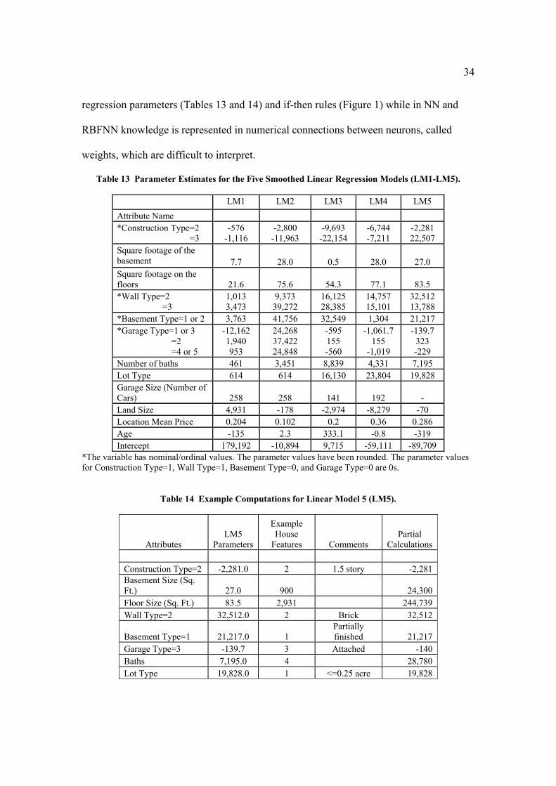
Table 13 Parameter Estimates for the Five Smoothed Linear Regression Models (LM1-LM5).

LM1 LM2 LM3 LM4 LM5 Attribute Name *Construction Type=2 =3

-576 -1,116

-2,800 -11,963

-9,693 -22,154

-6,744 -7,211

-2,281 22,507

Square footage of the basement 7.7 28.0 0.5 28.0 27.0 Square footage on the floors 21.6 75.6 54.3 77.1 83.5 *Wall Type=2 =3

1,013 3,473

9,373 39,272

16,125 28,385

14,757 15,101

32,512 13,788

*Basement Type=1 or 2 3,763 41,756 32,549 1,304 21,217 *Garage Type=1 or 3 =2 =4 or 5

-12,162 1,940 953

24,268 37,422 24,848

-595 155 -560

-1,061.7 155

-1,019

-139.7 323 -229

Number of baths 461 3,451 8,839 4,331 7,195 Lot Type 614 614 16,130 23,804 19,828 Garage Size (Number of Cars) 258 258 141 192 - Land Size 4,931 -178 -2,974 -8,279 -70 Location Mean Price 0.204 0.102 0.2 0.36 0.286 Age -135 2.3 333.1 -0.8 -319 Intercept 179,192 -10,894 9,715 -59,111 -89,709

*The variable has nominal/ordinal values. The parameter values have been rounded. The parameter values for Construction Type=1, Wall Type=1, Basement Type=0, and Garage Type=0 are 0s.

Table 14 Example Computations for Linear Model 5 (LM5).

Attributes LM5

Parameters

Example House

Features Comments Partial

Calculations Construction Type=2 -2,281.0 2 1.5 story -2,281 Basement Size (Sq. Ft.) 27.0 900 24,300 Floor Size (Sq. Ft.) 83.5 2,931 244,739 Wall Type=2 32,512.0 2 Brick 32,512

Basement Type=1 21,217.0 1 Partially finished 21,217

Garage Type=3 -139.7 3 Attached -140 Baths 7,195.0 4 28,780 Lot Type 19,828.0 1 <=0.25 acre 19,828

35

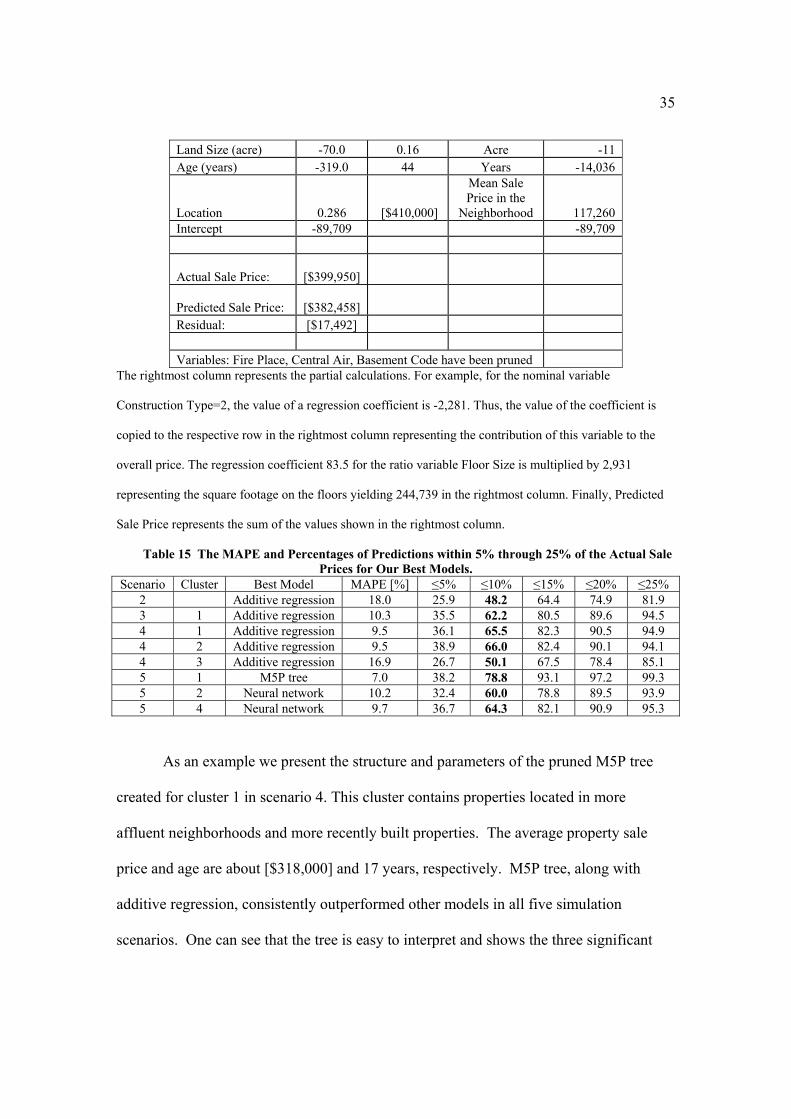
Land Size (acre) -70.0 0.16 Acre -11 Age (years) -319.0 44 Years -14,036

Location 0.286 [$410,000]

Mean Sale Price in the

Neighborhood 117,260 Intercept -89,709 -89,709

Actual Sale Price:

[$399,950]

Predicted Sale Price:

[$382,458] Residual: [$17,492] Variables: Fire Place, Central Air, Basement Code have been pruned

The rightmost column represents the partial calculations. For example, for the nominal variable

Construction Type=2, the value of a regression coefficient is -2,281. Thus, the value of the coefficient is

copied to the respective row in the rightmost column representing the contribution of this variable to the

overall price. The regression coefficient 83.5 for the ratio variable Floor Size is multiplied by 2,931

representing the square footage on the floors yielding 244,739 in the rightmost column. Finally, Predicted

Sale Price represents the sum of the values shown in the rightmost column.

Table 15 The MAPE and Percentages of Predictions within 5% through 25% of the Actual Sale Prices for Our Best Models.

Scenario Cluster Best Model MAPE [%] ≤5% ≤10% ≤15% ≤20% ≤25% 2 Additive regression 18.0 25.9 48.2 64.4 74.9 81.93 1 Additive regression 10.3 35.5 62.2 80.5 89.6 94.5 4 1 Additive regression 9.5 36.1 65.5 82.3 90.5 94.94 2 Additive regression 9.5 38.9 66.0 82.4 90.1 94.1 4 3 Additive regression 16.9 26.7 50.1 67.5 78.4 85.15 1 M5P tree 7.0 38.2 78.8 93.1 97.2 99.3 5 2 Neural network 10.2 32.4 60.0 78.8 89.5 93.95 4 Neural network 9.7 36.7 64.3 82.1 90.9 95.3

As an example we present the structure and parameters of the pruned M5P tree

created for cluster 1 in scenario 4. This cluster contains properties located in more

affluent neighborhoods and more recently built properties. The average property sale

price and age are about [$318,000] and 17 years, respectively. M5P tree, along with

additive regression, consistently outperformed other models in all five simulation

scenarios. One can see that the tree is easy to interpret and shows the three significant

36

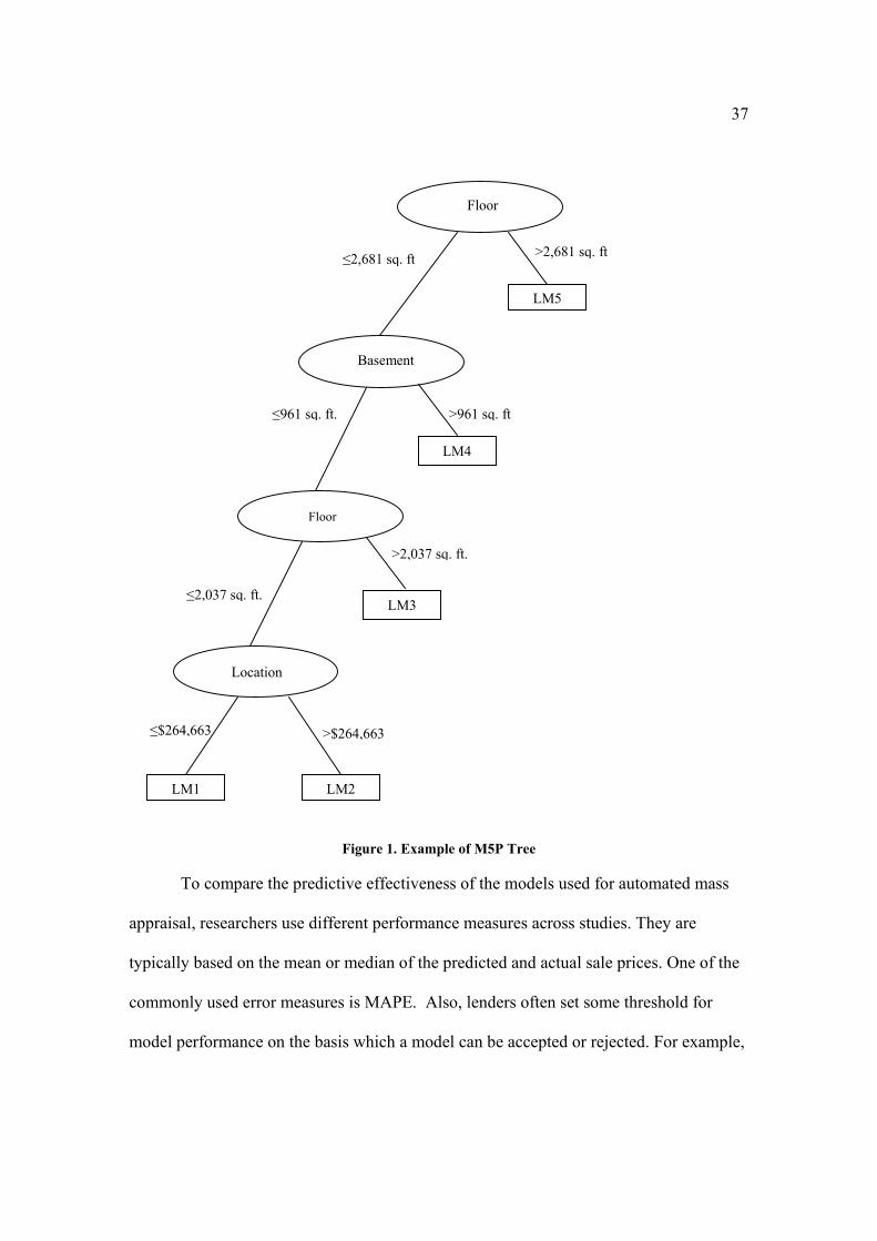
variables Floor, Basement (square footage on the floors and basement), and Location (the

average property sale price in the neighborhood). The branches and split values partition

the tree into 5 segments represented by five linear models. Depending on the input values

for the three variables, one of the five models is selected to calculate the predicted

property sale price. For example, if the Floor (the square footage on the floors) >2,681

sq. ft, the linear model 5 (LM5) is selected to estimate the property sale price (right top

branch of the tree). Similarly, if Floor ≤2,681 sq. ft., Basement ≤ 961 sq. ft, Floor ≤

2,037 sq. ft, and Location ≤[$264,663], the linear model 1 (LM1) is used. Tables 13 and

14 show the parameters of the 5 linear models and example calculations of the predicted

price, respectively. The signs of the regression parameters for the 5 linear models help

interpret the results. For example, the Floor, Basement, Baths, Lot Type, and Location

attributes have positive signs. This is a strength of the M5P method when compared with

black-box AI methods such as NN-based methods. As expected, the M5P tree also

discards relatively insignificant attributes such as Central Air and Fire Place (presence of

central air and fire place) as the vast majority of the properties in this cluster contain

these two features. The algorithm does not generate the values for their parameters

either.

37

Figure 1. Example of M5P Tree

To compare the predictive effectiveness of the models used for automated mass

appraisal, researchers use different performance measures across studies. They are

typically based on the mean or median of the predicted and actual sale prices. One of the

commonly used error measures is MAPE. Also, lenders often set some threshold for

model performance on the basis which a model can be accepted or rejected. For example,

Floor

LM5

>2,681 sq. ft

Basement

≤2,681 sq. ft

>961 sq. ft

LM4

≤961 sq. ft.

Floor

>2,037 sq. ft.

LM3

Location

LM1 LM2

>$264,663

≤2,037 sq. ft.

≤$264,663

38

Freddie Mac’s criterion states that on the test data, at least half of the predicted sale

prices should be within 10% of the actual prices (Fik, Ling, and Mulligan, 2003). We

calculated MAPE and the percentages of predictions within 5-25% of the actual sale

prices for our best models (Table 15). More than half of the models we created and

tested in this study were very close or exceeded the Freddie Mac 50% threshold (Table

15). In general, our models predict very well for the clusters of the properties built more

recently and located in high-end neighborhoods. In addition, our best model in scenario 2

created on the entire data set consisting of 16,366 transactions was quite close to the

Freddie Mac criterion and 48.2% of the predicted sale prices generated by this model

were within 10% of the actual sale prices.

8. Conclusion and Recommendations for Future Research

This paper describes the results of a comparative study that evaluates the

predictive performance of seven models for residential property value assessment. The

tested models include MRA, three non-traditional regression-based models, and three AI-

based models. The study represents the most comprehensive comparative study on a large

and very heterogeneous data sample. In addition to comparing NN, MRA, and MBR, we

have also introduced a variation of NN, i.e., RBFNN, and several methods relatively

unknown to the mass assessment community, i.e., additive regression, M5P tree, and

SVM-SMO. The simulation results clearly show that the nontraditional regression models

produce significantly better results than AI methods in various simulation scenarios,

especially in scenarios with more homogeneous data sets. The performance of these

nontraditional methods compares favorably with reported studies in terms of their MAPE

and R2 values though meaningful comparison is difficult for the reasons given earlier in

39

the paper. AI-based methods perform better for clusters containing more heterogeneous

data in some isolated simulation scenarios. None of the models perform well for low-end

and older properties. They generate relatively large prediction errors in those cases. We

believe that the relatively large prediction errors may be due to the fact that clusters with

low-end and older properties are very mixed in terms of sale prices, though not

necessarily in terms of property attributes values in the assessor's data set. Finally adding

“location” has substantially improved the prediction capability of the models. In this

study, “location” is defined as the mean sale price of the properties located in the same

district within the same neighborhood. In addition our data set also contains a group of

about 260 properties with large or very large land sizes ranging from 1 to 17.34 acres,

which also could have led to large prediction errors. This fact and possibly the use of

crisp K-means clustering may explain relatively low R2 values for several clusters in

scenarios 4 and 5 (Tables 11 and 12). Moreover, the MAPE measures for some of these

clusters are quite reasonable, exceeding the 50% threshold established by Freddie Mac

(Table 15).

There are several areas in which the reported study can be improved. First we

were restricted to attributes currently used by tax assessors, which exclude variables that

cannot be modeled by an MRA equation. But there could be other significant variables

that AI models would be able to process. Examples include age and condition of kitchen

and bathroom appliances/fixtures, views from the windows, brightness of the foyer,

condition and color of the paint, and quality of decorative molding. The incorporation of

this type of features in AI-based methods needs to be further investigated. Second,

refining the definition of “location” to represent the mean actual sale price of the

40

properties within a tax assessment block of houses could further enhance the predictive

capability of the models. It might be particularly helpful to introduce this more subtle and

modified definition of “location” for low-end and older properties. For example AI-based

methods can be used to better select/define the comparables that are used to calculate the

value of the location variable. The treatment of “location” in this paper is based on a

common practice by realtors and uses existing data from the local assessment office. This

definition of “location” has been shown to improve the results of the estimation in our

study. A possible area of future research is to incorporate more formal methods of spatial

analysis using externalities and spatial characteristics (Dubin, 1998; Gonzalez,

Soibelman, and Formoso, 2005; Kauko, 2003; Pace, Barry, and Sirmans, 1998;

Soibelman and Gonzalez, 2002). Recent studies of spatial analysis have shown clear

improvement of assessment accuracy (Bourassa, Cantoni, and Hoesli, 2010). These

results are consistent with our findings based on a more intuitive and simple definition of

“location”. Use of more formally defined and tested spatial analysis techniques,

especially those that lead to better disaggregated submarkets, may further improve

prediction results.

To magnify the effect of the house age, it might be reasonable to introduce the age

squared variable and try higher powers of age for building the models as was done in

several other studies. This comparative study has demonstrated the potential value of

nontraditional regression-based methods in mass assessment. Though the AI-based

methods tested in this study did not produce competitive results, other AI-based methods

need to be explored. For example Guan et al. (2008) found that combining neural

networks and fuzzy logic produced results comparable to MRA, but their findings suffer

41

from limited generalizability because of the small data set used for analysis (300

observations) and lack of diversity in property features (properties came from 2 modest

neighborhoods.) Another area of further research is to implement feature reduction

methods to increase the predictive capability and interpretability of the models. The

fewer the features are in a model, like the M5P structure in Figure 1, the better

understood the model is. We also recommend implementing fuzzy C-means clustering to

find more homogeneous segments of properties, especially for less affluent

neighborhoods and older properties. Employing a hybrid system might be a viable option

as well, i.e., using several models simultaneously and averaging their predicted sale

prices.

Thus we feel the findings in this study, with its large sample, variety of

techniques, and rigorous performance comparisons, will help improve understanding of

the strengths and weaknesses of various mass assessment approaches.

42

References Bagnoli, C. and H. C. Smith, The Theory of Fuzzy Logic and Its Application to Real

Estate Valuation, Journal of Real Estate Research, 1998, 16:2, 169-200.

Bonissone, P. P. and W. Cheetham, Financial Applications of Fuzzy Case-Based

Reasoning to Residential Property Valuation, Proceedings of Sixth International

Conference On Fuzzy Systems (FUZZ-IEEE’97), Barcelona, Spain, 1997, 37-44.

Bors, A. G., Introduction of the Radial Basis Function (RBF) Networks, OnLine

Symposium for Electronics Engineers, 2001, 1-7.

Boser, B., I. Guyon and V. Vapnik, A Training Algorithm for Optimal Margin

Classifiers, Proceedings of the Fifth Annual Workshop on Computational Learning

Theory, Pittsburgh, Pennsylvania, United States, 1992, 144-52.

Bourassa, S. C., E. Cantoni and M. Hoesli, Predicting House Prices with Spatial

Dependence: A Comparison of Alternative Methods, Journal of Real Estate Resach,

2010, 32:2, 139-59.

Byrne, P., Fuzzy Analysis: A Vague Way of Dealing with Uncertainty in Real Estate

Analysis?, Journal of Property Valuation and Investment, 1995, 13:3, 22-41.

Cui, D. and D. Curry, Prediction in Marketing Using the Support Vector Machine,

Marketing Science, 2005, 24:4, 595-615.

Do, A. Q. and G. Grudnitski, A Neural Network Approach to Residential Property

Appraisal, The Real Estate Appraiser, 1992, 58:3, 38–45.

43

Dubin, R., Spatial Autocorrelation: A Primer, Journal of Housing Economics, 1998, 7,

304-27.

Fik, T. J., D. C. Ling and G. F. Mulligan, Modeling Spatial Variation in Housing Prices:

A Variable Interaction Approach, Real Estate Economics, 2003, 31:4, 623 - 46.

Friedman, J., T. Hastie and R. Tibshirani, Additive Logistic Regression: A Statistical

View of Boosting (with Discussion Andrejoinder by the Authors), Annals of Statistics,

2000, 29:5, 337-407.

Gonzalez, A. J. and R. Laureano-Ortiz, A Case-Based Reasoning Approach to Real

Estate Property Appraisal, Expert Systems With Applications, 1992, 4:2, 229-46.

Gonzalez, M. A. S. and C. T. Formoso, Mass Appraisal with Genetic Fuzzy Rule-Based

Systems, Property Management, 2006, 24:1, 20-30.

Gonzalez, M. A. S., L. Soibelman and C. T. Formoso, A New Approach to Spatial

Analysis in CAMA, Property Management, 2005, 23:5, 312-27.

Guan, J. and A. S. Levitan, Artificial Neural Network Based Assessment of Residential

Real Estate Property Prices: A Case Study, Accounting Forum, 1997, 20:3/4, 311-26.

Guan, J., J. Zurada and A. S. Levitan, An Adaptive Neuro-Fuzzy Inference System Based

Approach to Real Estate Property Assessment, Journal of Real Estate Research, 2008,

30:4, 395-420.

Jang, J. S. R., ANFIS: Adaptive-Network-Based Fuzzy Inference System, IEEE

Transactions on Systems, Man, and Cybernetics, 1993, 23:3, 665-85.

44

Kauko, T., Residential Property Value and Locational Externalities, Journal of Property

Investment and Finance, 2003, 21:3, 250–70.

Krol, D., T. Lasota, W. Nalepa and B. Trawinski, Fuzzy System Model to Assist with

Real Estate Appraisals, Lecture Notes in Computer Science, 2007, 4570, 260-69.

Larsen, J. E. and M. O. Peterson, Correcting for Errors in Statistical Appraisal Equations,

The Real Estate Appraiser and Analyst, 1988, 54:3, 45-49.

Limsombunchai, V., C. Gan and M. Lee, House Price Prediction: Hedonic Price Model

Vs. Artificial Neural Network, American Journal of Applied Sciences, 2004, 1:3, 193-

201.

Mark, J. and M. Goldberg, Multiple Regression Analysis and Mass Assessment: A

Review of the Issues, Appraisal Journal, 1988, 56:1, 89-109.

McCluskey, W. and S. Anand, The Application of Intelligent Hybrid Techniquesfor the

Mass Appraisal of Residential Properties, Journal of Property Investment and Finance,

1999, 17:3, 218-38.

McGreal, S., A. Adair, D. McBurney and D. Patterson, Neural Networks: The Prediction

of Residential Values, Journal of Property Valuation and Investment, 1998, 16, 57-70.

Newsome, B. A. and J. Zietz, Adjusting Comparable Sales Using Multiple Regression

Analysis--the Need for Segmentation, The Appraisal Journal, 1992, 60:1, 129--33.

45

Nguyen, N. and A. Cripps, Predicting Housing Value: A Comparison of Multiple

Regression Analysis and Artificial Neural Networks, Journal of Real Estate Research,

2002, 22:3, 313-36.

Osuna, E., R. Freund and F. Girosi, An Improved Training Algorithm for Support Vector

Machines, Proceedings of the 1997 IEEE Workshop on Neural Networks for Signal

Processing, Amelia Island, Florida, 1997, 276–85.

Pace, R., R. Barry and C. Sirmans, Spatial Statistics and Real Estate, The Journal of Real

Estate Finance and Economics, 1998, 17:1, 5-13.

Park, J. and J. W. Sandberg, Universal Approximation Using Radial Basis Functions

Network, Neural Computation, 1991, 3, 246-57.

Peterson, S. and A. B. Flanagan, Neural Network Hedonic Pricing Models in Mass Real

Estate Appraisal, Journal of Real Estate Research, 2009, 31:2, 147-64.

Poggio, T. and F. Girosi, Networks for Approximation and Learning, Proceedings of

IEEE, 1990, 78:9, 1481-97.

Quinlan, J. R., Learning with Continuous Classes, Proceedings of the 5th Australian Joint

Conference on Artificial Intelligence, Singapore, 1992, 343–48.

Rossini, P., Artificial Neural Networks Versus Multiple Regression in the Valuation of

Residential Property, Australian Land Economics Review, 1997, 3:1, 1-12.

46

Soibelman, L. and M. A. S. Gonzalez, A Knowledge Discovery in Databases Framework

for Property Valuation, Journal of Property Tax Assessment and Administration, 2002,

7:2, 77-104.

Taffese, W. Z., Case-Based Reasoning and Neural Networks for Real Estate Valuation,

Proceedings of the 25th Conference on Proceedings of the 25th IASTED International

Multi-Conference: Artificial Intelligence and Applications, Innsbruck, Austria, 2007, 84-

89.

Vapnik, V. N., Statistical Learning Theory, New York: Wiley, 1998.

Viaene, S., R. A. Derrig, B. Baesens and G. Dedene, A Comparison of State-of-the-Art

Classification Techniques for Expert Automobile Insurance Claim Fraud Detection,

Journal of Risk Insurance, 2002, 63:3, 373-421.

Wang, Y. and I. Witten, Inducing Model Trees for Continuous Classes, Proceedings of

Poster Papers, Ninth European Conference on Machine Learning, Prague, Czech

Republic, 1997, 128–37.

Witten, I. H. and E. Frank, Data Mining: Practical Machine Learning Tools and

Techniques, San Francisco: Morgan Kaufmann, 2005.

Worzala, E., M. Lenk and A. Silva, An Exploration of Neural Networks and Its

Application to Real Estate Valuation, Journal of Real Estate Research, 1995, 10, 185-

202.

47

Acknowledgement We are grateful to the Jefferson County Property Valuation Administrator, who provided

the data used in this study.