A comparison of perfromance in selected US and European … · Jim RIES (FAA) Bernd SCHUH (DFS) Riccardo SPADONI (ENAV) Peter TULLETT (NATS) Frans VAN GYSEGEM (Maastricht) Table of

Acknowledgements

The Performance Review Unit (PRU) would like to acknowledge the invaluablecontribution made by the participants in the ACE/US-Europe Centres ComparisonsWorking Group who ensured that high-quality information was provided, andvalidated the interpretations contained in this report. In particular, the PRU would liketo thank:

Arthur BENZLE (FAA)David BOONE (FAA)Francisco DE LA PLAZA BODALO (Aena)Klaas de VRIES (Maastricht)Nadio di RIENZO (ENAV)Michael GAMBONE (FAA)Jean-Claude GOUHOT (DNA)John HENNIGAN (FAA)Ralf HOELSCHER (Maastricht)Richard KETTELL (FAA)Thomas KLEIN (DFS)Nicolas LOCHANSKI (DNA)Thomas MAKIES (DFS)Joan MALLEN (FAA)Frédéric MEDIONI (DNA)Penny MEFFORD (FAA)Werner NASEMANN (DFS)Francisco ORTIZ (Aena)Fernando REBOLLO (Aena)Jim RIES (FAA)Bernd SCHUH (DFS)Riccardo SPADONI (ENAV)Peter TULLETT (NATS)Frans VAN GYSEGEM (Maastricht)

Table of contents

Executive Summary............................................................................................................. i1 Main findings of the study .............................................................................. i2 Origin and scope of the study......................................................................... ii3 The comparison.............................................................................................. ii4 Factors behind the performance gap ............................................................. iii

1 Introduction ...............................................................................................................11.1 The origin of the study ....................................................................................11.2 Scope of the study ...........................................................................................21.3 Safety...............................................................................................................41.4 Quality of service ............................................................................................41.5 Participation in the study.................................................................................51.6 Working methods ............................................................................................51.7 Selection of the centres ...................................................................................7

2 Description of selected centres ..................................................................................92.1 Introduction .....................................................................................................92.2 Comparison of key features.............................................................................92.3 Barcelona ACC .............................................................................................122.4 Karlsruhe UAC..............................................................................................132.5 London ACC .................................................................................................142.6 Maastricht UAC ............................................................................................152.7 Reims ACC ...................................................................................................162.8 Roma ACC ....................................................................................................172.9 Albuquerque ARTCC....................................................................................182.10 Cleveland ARTCC ........................................................................................192.11 Indianapolis ARTCC.....................................................................................20

3 How we are comparing performance.......................................................................233.1 Introduction ...................................................................................................233.2 Outputs, inputs and overall cost-effectiveness ..............................................233.3 The analytical framework..............................................................................253.4 Data sources ..................................................................................................27

4 Review of results .....................................................................................................294.1 Introduction ...................................................................................................294.2 Operational cost-effectiveness ......................................................................294.3 ATCO-hour productivity...............................................................................304.4 ATCO working hours....................................................................................314.5 ATCO employment costs ..............................................................................334.6 Support cost...................................................................................................344.7 Conclusions ...................................................................................................35

5 Traffic complexity and variability...........................................................................395.1 Introduction ...................................................................................................395.2 Traffic complexity.........................................................................................395.3 Traffic variability ..........................................................................................43

6 Influences on output per ATCO ..............................................................................516.1 The components of output per ATCO...........................................................516.2 ATCO working hours....................................................................................516.3 ATCO-hour productivity...............................................................................53

6.4 Conclusions on output per ATCO.................................................................61

7 Flexibility in the use of resources............................................................................637.1 Introduction ...................................................................................................637.2 Our findings ..................................................................................................637.3 Flexibility from rostering practices ...............................................................647.4 Dealing with seasonal variation ....................................................................657.5 Dealing with within-week variation..............................................................667.6 Dealing with hourly variation .......................................................................677.7 Conclusions ...................................................................................................72

8 Support cost differences ..........................................................................................738.1 Introduction ...................................................................................................738.2 The composition of support costs..................................................................738.3 Support staff ..................................................................................................758.4 Conclusions on support costs ........................................................................78

9 ATFM differences ...................................................................................................799.1 Introduction ...................................................................................................799.2 Different ATM contexts ................................................................................799.3 The ATFM system in Europe........................................................................809.4 The ATFM system in the USA .....................................................................819.5 Review of significant differences..................................................................849.6 Conclusions ...................................................................................................86

10 Other factors influencing performance....................................................................8910.1 Introduction ...................................................................................................8910.2 Influences identified in the operational exchange programme......................8910.3 Military practices ..........................................................................................9010.4 ATM technology, data flow and working methods.......................................9110.5 Airspace design .............................................................................................9210.6 Conclusions ...................................................................................................92

11 Conclusions and comparison with overall performance..........................................9311.1 Introduction ...................................................................................................9311.2 Sources of the difference...............................................................................9311.3 Influences on performance differences .........................................................9411.4 Further areas to explore.................................................................................95

Glossary .............................................................................................................................97

ANNEX A: Factsheets for the centres selected ................................................................99

List of figures

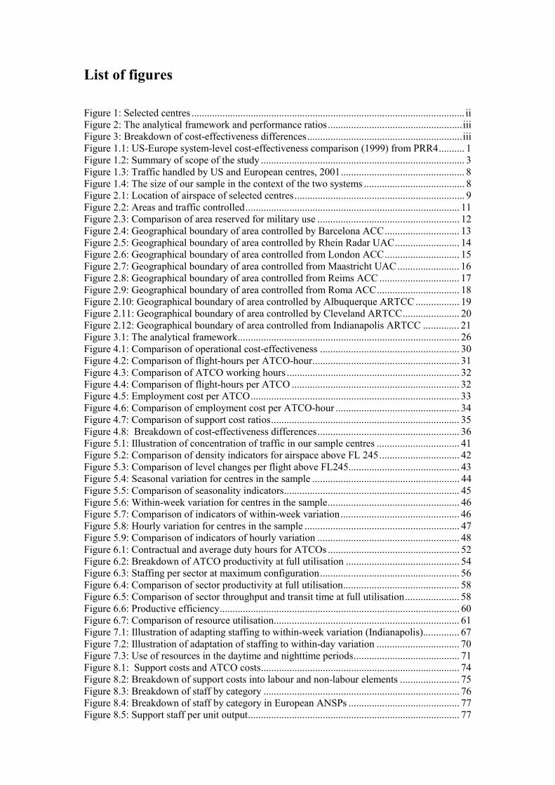
Figure 1: Selected centres .......................................................................................................... iiFigure 2: The analytical framework and performance ratios....................................................iiiFigure 3: Breakdown of cost-effectiveness differences............................................................iiiFigure 1.1: US-Europe system-level cost-effectiveness comparison (1999) from PRR4.......... 1Figure 1.2: Summary of scope of the study ............................................................................... 3Figure 1.3: Traffic handled by US and European centres, 2001................................................ 8Figure 1.4: The size of our sample in the context of the two systems ....................................... 8Figure 2.1: Location of airspace of selected centres.................................................................. 9Figure 2.2: Areas and traffic controlled................................................................................... 11Figure 2.3: Comparison of area reserved for military use ....................................................... 12Figure 2.4: Geographical boundary of area controlled by Barcelona ACC............................. 13Figure 2.5: Geographical boundary of area controlled by Rhein Radar UAC......................... 14Figure 2.6: Geographical boundary of area controlled from London ACC............................. 15Figure 2.7: Geographical boundary of area controlled from Maastricht UAC........................ 16Figure 2.8: Geographical boundary of area controlled from Reims ACC ............................... 17Figure 2.9: Geographical boundary of area controlled from Roma ACC................................ 18Figure 2.10: Geographical boundary of area controlled by Albuquerque ARTCC ................. 19Figure 2.11: Geographical boundary of area controlled by Cleveland ARTCC...................... 20Figure 2.12: Geographical boundary of area controlled from Indianapolis ARTCC .............. 21Figure 3.1: The analytical framework...................................................................................... 26Figure 4.1: Comparison of operational cost-effectiveness ...................................................... 30Figure 4.2: Comparison of flight-hours per ATCO-hour......................................................... 31Figure 4.3: Comparison of ATCO working hours ................................................................... 32Figure 4.4: Comparison of flight-hours per ATCO ................................................................. 32Figure 4.5: Employment cost per ATCO................................................................................. 33Figure 4.6: Comparison of employment cost per ATCO-hour ................................................ 34Figure 4.7: Comparison of support cost ratios......................................................................... 35Figure 4.8: Breakdown of cost-effectiveness differences....................................................... 36Figure 5.1: Illustration of concentration of traffic in our sample centres ................................ 41Figure 5.2: Comparison of density indicators for airspace above FL 245............................... 42Figure 5.3: Comparison of level changes per flight above FL245........................................... 43Figure 5.4: Seasonal variation for centres in the sample ......................................................... 44Figure 5.5: Comparison of seasonality indicators.................................................................... 45Figure 5.6: Within-week variation for centres in the sample................................................... 46Figure 5.7: Comparison of indicators of within-week variation.............................................. 46Figure 5.8: Hourly variation for centres in the sample ............................................................ 47Figure 5.9: Comparison of indicators of hourly variation ....................................................... 48Figure 6.1: Contractual and average duty hours for ATCOs ................................................... 52Figure 6.2: Breakdown of ATCO productivity at full utilisation ............................................ 54Figure 6.3: Staffing per sector at maximum configuration...................................................... 56Figure 6.4: Comparison of sector productivity at full utilisation............................................. 58Figure 6.5: Comparison of sector throughput and transit time at full utilisation..................... 58Figure 6.6: Productive efficiency............................................................................................. 60Figure 6.7: Comparison of resource utilisation........................................................................ 61Figure 7.1: Illustration of adapting staffing to within-week variation (Indianapolis).............. 67Figure 7.2: Illustration of adaptation of staffing to within-day variation ................................ 70Figure 7.3: Use of resources in the daytime and nighttime periods......................................... 71Figure 8.1: Support costs and ATCO costs............................................................................. 74Figure 8.2: Breakdown of support costs into labour and non-labour elements ....................... 75Figure 8.3: Breakdown of staff by category ............................................................................ 76Figure 8.4: Breakdown of staff by category in European ANSPs ........................................... 77Figure 8.5: Support staff per unit output.................................................................................. 77

i

Executive Summary

1 Main findings of the study

US centres are more cost-effective

A comparison of selected US and European en-routecentres has found that the US centres aresignificantly more cost-effective. While the resultsfrom the different centres (Barcelona, Karlsruhe,London, Maastricht, Reims and Roma in Europe,Albuquerque, Cleveland and Indianapolis in the US)are diverse, the operating costs per flight-hourcontrolled in the selected European centres were, onaverage, more than 60% higher than those in theselected US centres.

A benchmarking framework, developed for thepurposes of this comparison, has broken down thisdifference into two main factors, each accounting foraround half the difference:

(a) US controllers handle more flight-hours; and

(b) support costs at the centres (those costs otherthan the costs of the controllers themselves) arehigher in Europe.

The framework, developed in collaboration with allthe service providers concerned, was the result of thefirst large-scale co-operative comparative exercise ata detailed level between providers, and has provedhighly effective in helping to identify major causesof difference and deepening understanding of keybusiness processes.

One should refrain from drawing rapid conclusionsfrom comparative analyses, which are necessarilynot exhaustive. Indeed, even though manysimilarities exist between the US and the EuropeanATM systems, different legal, economic, social,cultural and operational environments may explainpart or all of observed differences. In this report, adistinction is made between factual findings, whichhave been checked extensively and are as accurateas possible, and performance drivers which mayexplain the differences.

US controllers have higher productivity

US controllers handle more traffic in part becausethey work significantly more hours than theirEuropean counterparts. This factor is compensatedfor by the fact that the cost of employing controllers

is higher in the US; taking these two effectstogether, the cost per working hour is around thesame in the US as in Europe.

The difference in controller productivity arises inpart from the fact that the US controllers can handlemore traffic when working at their maximumthroughput, and in part from the fact that theavailability of US controllers to staff the operationsroom is better matched to the ups and downs oftraffic leading to better resources utilisation.

Differences in working, operational, andorganisational practices lie behind these differencesin performance:

• US management has access to a greater varietyof practices that allow them to deploycontrollers with greater flexibility to adapt totraffic variation.

• Differences in the way that Air Traffic FlowManagement and civil-military co-operation areorganised help controllers be more productive inthe US.

• The US operates on a uniform system; hand-overs between centres are no more difficult thanhand-overs within a centre, reducing controllerworkload.

Although complexity was found to have an impacton productivity, there is no evidence of a systemicdifference in traffic complexity between the selectedUS and European en-route centres.

Support costs are higher in Europe

Support costs � the costs other than those foremploying controllers � also make a majorcontribution to the observed performance gap.These are associated largely with higher numbers ofnon-controller staff in the European centres. In mostEuropean centres, non-staff operating costs arehigher per unit output as well.

This difference, discovered as a result of this study,deserves attention at the service provider level aswell; the differences in support costs may be evenlarger when costs at service provider headquartersare taken into account.

The remainder of this Executive Summary describeshow these findings were made; more detail isavailable in the full Report.

ii

2 Origin and scope of the study

The PRC�s Fourth Performance Review Report inApril 2001 (PRR4) identified significant differencesin performance between the US and European ATMSystems in the year 1999. The �gate-to-gate� costsof providing air navigation services (ANS),including all en-route and terminal navigation costs,per km flown, were, on average, 70% higher inEurope than in the US.

In July 2001, the Provisional Council ofEUROCONTROL encouraged the PRC toinvestigate this comparison further and �requestedMember States to encourage their ANS providers toparticipate actively in the benchmarking exercisebeing undertaken by the PRC in cooperation withthe interested parties�.

This detailed comparative study was conducted bythe PRU in close collaboration with the sixEuropean ANSPs1 and the US Federal AviationAdministration (FAA). A Working Groupcomprising the PRU and representatives from thevarious ANSPs, including operational and financialexperts, had five meetings over the period February2002 to March 2003. This Report is the product ofthis collaborative work.

The scope of the study was to analyse performanceat a selection of individual en-route area air trafficcontrol centres in the US and Europe and see to whatextent the cost-effectiveness differences identified atsystem level in PRR4 arose from differences at thelevel of the basic operating units. The focus of thestudy was on identification of systemic differencesbetween European centres as a whole and UScentres as a whole, rather than on comparingindividual centres with each other.

The study does not address nor compare safetyissues. There is no evidence from available data toshow any difference in ATM safety performancebetween the US and European ATM systems.Similarly, the study does not address nor comparequality of services provided to users. The methodsof measuring delay, the chief element of quality ofservice, were not readily comparable betweenEurope and the US.

1 Aena, DFS, DNA, ENAV, EUROCONTROL Maastricht, andNATS.

We wished to choose centres that werehomogeneous in their size and scope of activities.This meant choosing larger European centres, sincethe US centres tend to be large. We also chosecentres where the principal activity was in upperairspace, since US en-route centres do not cover theapproaches to airports.

The six European centres and three US centreschosen are shown in Figure 1.

Figure 1: Selected centres

The selected centres account for about 19% and 12%of the flight hours controlled in the European and theUS systems respectively.

To facilitate the comparison at centre level, we wereselective about the categories of cost included. Onlythe direct operating costs for ATM provision wereconsidered. Capital-related costs (finance costs anddepreciation), maintenance costs for the CNSinfrastructure, and HQ support costs were notincluded. The costs associated with the selectedEuropean centres and US centres account for about7% of the total en-route costs.

3 The comparison

To undertake this comparison of centres, wedeveloped a detailed framework for analysing andbenchmarking indicators of operational andeconomic performance between centres. Thisframework has proved highly effective inunderstanding and explaining aggregateperformance comparisons.

To understand how differences in the operationalcost-effectiveness ratio arise, we broke it down intoa number of component ratios, as shown in Figure 2.By convention, a ratio higher than 1 means a betterUS performance.

iii

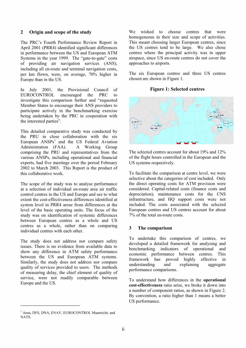
Figure 2: The analytical framework andperformance ratios

Flight-hours controlled

ATCO-hours on operational duty

ATCOs in operations

Employment costs of operational ATCOs

Total operating costs(staff and non-staff)

Cost-effectiveness

Productivity and factor cost

� ATCO-hour productivity

1.29

� working hours per ATCO 1.32

� employment cost per ATCO 0.71

� support cost ratio 1.34

� operating costs per flight-hour controlled

1.62� employment cost

per ATCO-hour0.94



ATCOs in operations



Cost-effectiveness



1.29

� working hours per ATCO 1.32

� employment cost per ATCO 0.71

� support cost ratio 1.34


1.62� employment cost

per ATCO-hour0.94

Figure 2 indicates the performance ratios for each ofthe elements in the framework.

The average operating cost per flight-hour at theEuropean centres is 62% more than that in our USsample. The systemic difference is striking: theoperating costs at the European centres we havechosen are well over those in the US centres. Thisdifference results from two major effects:

1. On average, each ATCO on operational duty inthe US centres handles on average 29% moreflight-hours per hour on duty than the averageEuropean - a performance ratio of 1.29. Inaddition, ATCOs in the US work on average32% more hours. Taken together, these twofactors mean that the average European ATCOcontrols around 1700 flight-hours a year,whereas the corresponding ATCO in the UScentres controls 2900 flight-hours; a ratio of1.70.

2. Support costs � all the operating costs in thecentre other than the employment costs ofATCOs � are greater in Europe than in the US.On average the ratio of total operating costs tothe employment costs of ATCOs is 34% higherin our European sample than in our US sample.

While the employment costs of ATCOs are around41% greater in our US sample than in our Europeansample (a performance ratio of 0.71), this iscompensated for by the fact that US ATCOs workmore hours. Taking these two factors together, wefind that the performance ratio resulting fromemployment costs is 0.94; the cost per ATCO-houris 0.94 in our European sample of what it is in ourUS sample.

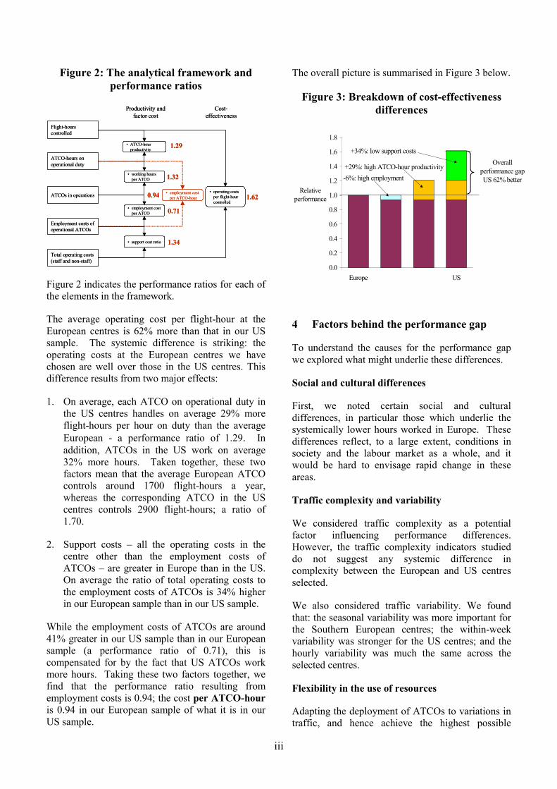
The overall picture is summarised in Figure 3 below.

Figure 3: Breakdown of cost-effectivenessdifferences

0.0

0.2

0.4

0.6

0.8

1.0

1.2

1.4

1.6

1.8

Europe US

Relative performance

-6%: high employment

+34%: low support costs

+29%: high ATCO-hour productivity Overall performance gap US 62% better

4 Factors behind the performance gap

To understand the causes for the performance gapwe explored what might underlie these differences.

Social and cultural differences

First, we noted certain social and culturaldifferences, in particular those which underlie thesystemically lower hours worked in Europe. Thesedifferences reflect, to a large extent, conditions insociety and the labour market as a whole, and itwould be hard to envisage rapid change in theseareas.

Traffic complexity and variability

We considered traffic complexity as a potentialfactor influencing performance differences.However, the traffic complexity indicators studieddo not suggest any systemic difference incomplexity between the European and US centresselected.

We also considered traffic variability. We foundthat: the seasonal variability was more important forthe Southern European centres; the within-weekvariability was stronger for the US centres; and thehourly variability was much the same across theselected centres.

Flexibility in the use of resources

Adapting the deployment of ATCOs to variations intraffic, and hence achieve the highest possible

iv

resource utilisation, requires working practices thatallow for flexibility. Some 23% of the performancegap between the US and Europe arises from theability of US centres to adapt their staffing better tothe traffic variability that they face.

Staff planning and management is not alwaysdesigned to match traffic. In many centres rostershave remained unchanged for some years and certainpractices appear to be imperfectly adapted to currentpatterns of traffic variation. In some cases, therewere clear indications that adopting better practicesfrom other ANSPs in our sample might bringimprovements.

Support costs

A major component of the difference in cost-effectiveness at centre level is differences in�support costs� � that is, the costs that a centrespends on items other than the employment ofATCOs. Support costs in Europe are 34% higher.

A major cause of the difference appears to be thenumbers of non-ATCO staff in certain Europeancentres. Moreover, non-labour support costs in theEuropean centres are consistently as high or higherthan in the US centres.

Air Traffic Flow Management (ATFM)procedures

While they share the same objectives of safety andefficiency, the US and Europe have radicallydifferent approaches to ATFM:

• in the US, ATFM measures are determined andimposed within a few hours, whereas in Europethey tend to be planned 24 hours in advance.

• In the US, a variety of possible ATFMprocedures are available, which can be tailoredto the problem to be addressed. Ground delay,the predominant procedure in Europe, isconsidered as a last resort measure in the US.

• There is an on-going collaborative decisionmaking process, involving all US ATFMstakeholders. Options are discussed withairspace users.

• ATFM is much more decentralised in the US.Typically, in a US centre, 6 to 8 trafficcontrollers are responsible for flow managementmeasures throughout the day.

While it is difficult to quantify any comparison, itappears that the US ATFM system positivelycontributes to the productivity gap found in thisReport.

Other areas

In a number of other areas, we were able to identifypractices that were likely to contribute towards thedifferences in cost-effectiveness, although the causallink was harder to prove. These included:

• civil-military co-operation processes: moreintegrated and more effective civil-militaryarrangements in the US.

• interoperability between systems; we werestruck by the statement that hand-over betweencentres in the US required no more controllereffort than hand-over between sectors. Thisdifference in hand-over workload would make adifference to the productive efficiency of sectorsand hence ATCOs.

1

1 Introduction

1.1 The origin of the study

The Performance Review Commission of EUROCONTROL (the PRC) has, as part ofits terms of reference, a requirement to �propose overall objectives for improvementof the ATM system performance for approval by the Permanent Commission throughthe Provisional Council (Art. 10. a)�. In fulfilment of this, it has an interest in ATMservice provision in countries outside Europe and how European performancecompares with that of other providers worldwide.

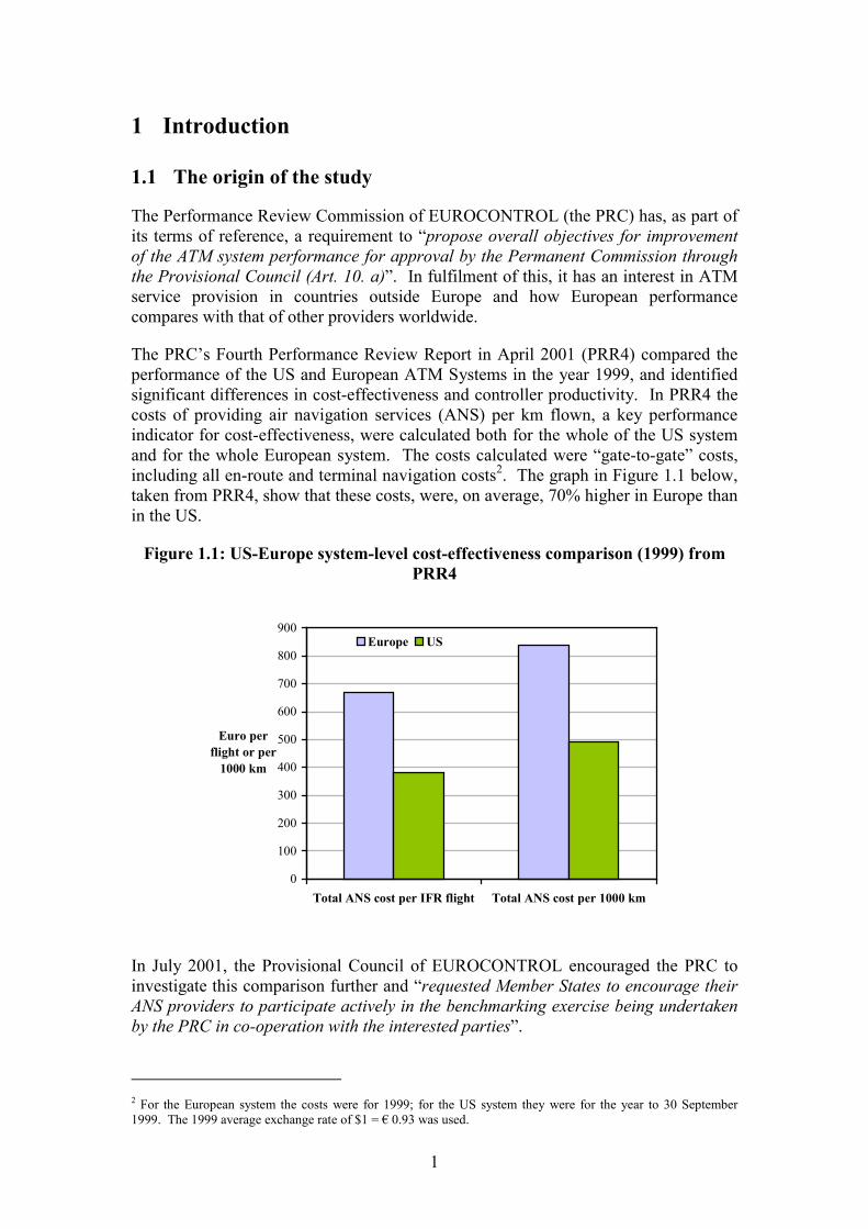
The PRC�s Fourth Performance Review Report in April 2001 (PRR4) compared theperformance of the US and European ATM Systems in the year 1999, and identifiedsignificant differences in cost-effectiveness and controller productivity. In PRR4 thecosts of providing air navigation services (ANS) per km flown, a key performanceindicator for cost-effectiveness, were calculated both for the whole of the US systemand for the whole European system. The costs calculated were �gate-to-gate� costs,including all en-route and terminal navigation costs2. The graph in Figure 1.1 below,taken from PRR4, show that these costs, were, on average, 70% higher in Europe thanin the US.

Figure 1.1: US-Europe system-level cost-effectiveness comparison (1999) fromPRR4

0

100

200

300

400

500

600

700

800

900

Total ANS cost per IFR flight Total ANS cost per 1000 km

Euro perflight or per

1000 km

Europe US

In July 2001, the Provisional Council of EUROCONTROL encouraged the PRC toinvestigate this comparison further and �requested Member States to encourage theirANS providers to participate actively in the benchmarking exercise being undertakenby the PRC in co-operation with the interested parties�.

2 For the European system the costs were for 1999; for the US system they were for the year to 30 September1999. The 1999 average exchange rate of $1 = � 0.93 was used.

2

The PRC requested that the Performance Review Unit (PRU) undertake a moredetailed comparative study, with the cooperation of a number of European airnavigation service providers (ANSPs) and the US Federal Aviation Administration(FAA). The study was conducted over the period February 2002 to March 2003. Thisis the report of its findings.

The structure of the report is as follows:

• the remainder of this introduction discusses the scope of the study and themethods adopted;

• Chapter 2 presents an overview of the centres selected for comparison;

• Chapter 3 describes the analytical framework we have adopted;

• Chapter 4 discusses the quantitative results from our comparison ofoperational cost-effectiveness;

• Chapter 5 compares the traffic complexity and variability in the centres;

• Chapter 6 looks in more detail at the comparison of ATCO productivity and atsome of the factors that might underlie the observed differences;

• Chapter 7 examines working practices and their impact on the flexibility in theuse of resources;

• Chapter 8 looks in more detail at the support cost differences;

• Chapter 9 examines how differences in ATFM practices might contribute toobserved differences in performance;

• Chapter 10 examines other factors that might influence various aspects ofperformance; and

• Chapter 11 presents our conclusions in the light of the previous work shown inPRR4.

Annex A contains factsheets on each en-route centre that give more detaileddescriptions.

1.2 Scope of the study

The scope of the study comprised a selection of individual en-route area air trafficcontrol centres in the US and Europe. The objective of the work was to see to whatextent the differences identified at system level in PRR4 arose from differences at thelevel of the basic operating units. If this was the case, the study would try to identifyat which stage of the �production� process the differences arose, and what differences,either in practices or exogenous conditions, caused them.

The study does not address or compare safety issues, for reasons that are discussed inSection 1.3. Nor does it compare the quality of service provided to users, asexplained in Section 1.4.

3

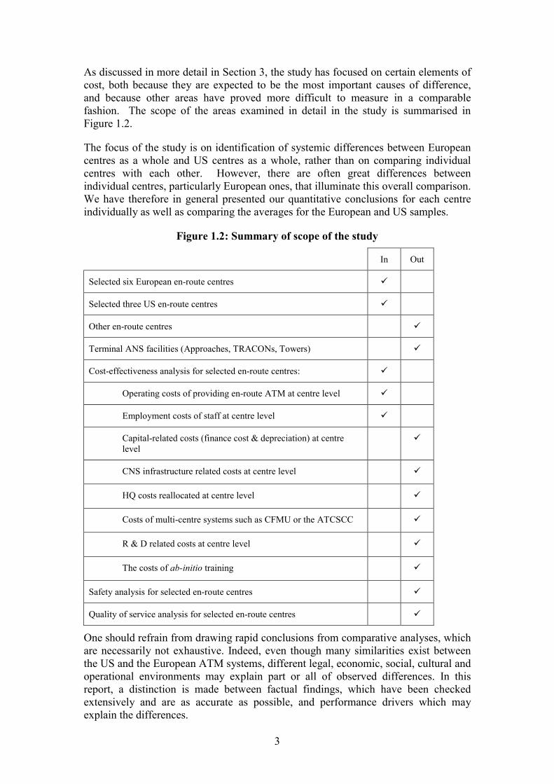
As discussed in more detail in Section 3, the study has focused on certain elements ofcost, both because they are expected to be the most important causes of difference,and because other areas have proved more difficult to measure in a comparablefashion. The scope of the areas examined in detail in the study is summarised inFigure 1.2.

The focus of the study is on identification of systemic differences between Europeancentres as a whole and US centres as a whole, rather than on comparing individualcentres with each other. However, there are often great differences betweenindividual centres, particularly European ones, that illuminate this overall comparison.We have therefore in general presented our quantitative conclusions for each centreindividually as well as comparing the averages for the European and US samples.

Figure 1.2: Summary of scope of the study

In Out

Selected six European en-route centres �

Selected three US en-route centres �

Other en-route centres �

Terminal ANS facilities (Approaches, TRACONs, Towers) �

Cost-effectiveness analysis for selected en-route centres: �

Operating costs of providing en-route ATM at centre level �

Employment costs of staff at centre level �

Capital-related costs (finance cost & depreciation) at centrelevel

�

CNS infrastructure related costs at centre level �

HQ costs reallocated at centre level �

Costs of multi-centre systems such as CFMU or the ATCSCC �

R & D related costs at centre level �

The costs of ab-initio training �

Safety analysis for selected en-route centres �

Quality of service analysis for selected en-route centres �

One should refrain from drawing rapid conclusions from comparative analyses, whichare necessarily not exhaustive. Indeed, even though many similarities exist betweenthe US and the European ATM systems, different legal, economic, social, cultural andoperational environments may explain part or all of observed differences. In thisreport, a distinction is made between factual findings, which have been checkedextensively and are as accurate as possible, and performance drivers which mayexplain the differences.

4

1.3 Safety

Safety is of paramount importance in the provision of air navigation services, andproviding the requisite level of safety is a vital and overriding element in quality ofservice.

We have no way of measuring safety in a comparable way between the variouscentres. We do not believe that any of the ANSPs studied would conceivably makedecisions to reduce safety levels to increase the direct cost-effectiveness. No trade-offs would be made with safety.

Our position in this study is therefore that we are not addressing or comparing levelsof safety; we are assuming that each ANSP is ensuring and will continue to ensurethat requisite safety levels are met and maintained, and that any improvements in cost-effectiveness or the non-safety elements of quality of service are made while stillsatisfying the constraint that safety levels are not diminished. There is no evidence toshow any systemic difference in ATM safety performance between the US andEuropean ATM systems.

1.4 Quality of service

This study has not examined the quality of the service that the ANSP provides tousers. At an early stage, we found that the methods of measuring delay, the chiefelement of quality of service, were not comparable between Europe and the US. If wewished to fairly and consistently compare the delay induced by air traffic managementbetween Europe and the US, we would need:

(a) to define a common and consistent measure of delay; and

(b) to collect the data that would allow us to measure it.

This would be a very substantial exercise, requiring resources and timescales wellbeyond those available for this study.

We have therefore taken a narrower measure of cost-effectiveness as the basis forcomparison in this study � we are comparing the direct cost-effectiveness of providingthe service that is currently provided by each centre, and not including a comparisonof the effectiveness of that level of service in meeting users� needs.

It is important, however, to bear in mind that differences in performance as measuredby cost-effectiveness and productivity may well be accompanied by differences inquality of service, even though we cannot consistently measure them at present.There is no evidence, however, of any differences in the quality of service provided tousers at the system level. Table 1.1 below, which shows the main punctualityindicators, suggests that the quality of service is not systemically different.

5

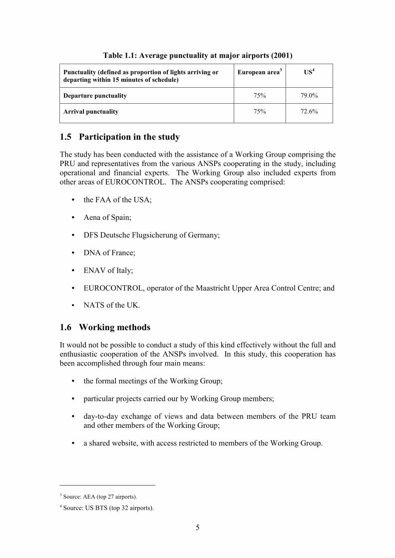
Table 1.1: Average punctuality at major airports (2001)

Punctuality (defined as proportion of lights arriving ordeparting within 15 minutes of schedule)

European area3 US4

Departure punctuality 75% 79.0%

Arrival punctuality 75% 72.6%

1.5 Participation in the study

The study has been conducted with the assistance of a Working Group comprising thePRU and representatives from the various ANSPs cooperating in the study, includingoperational and financial experts. The Working Group also included experts fromother areas of EUROCONTROL. The ANSPs cooperating comprised:

• the FAA of the USA;

• Aena of Spain;

• DFS Deutsche Flugsicherung of Germany;

• DNA of France;

• ENAV of Italy;

• EUROCONTROL, operator of the Maastricht Upper Area Control Centre; and

• NATS of the UK.

1.6 Working methods

It would not be possible to conduct a study of this kind effectively without the full andenthusiastic cooperation of the ANSPs involved. In this study, this cooperation hasbeen accomplished through four main means:

• the formal meetings of the Working Group;

• particular projects carried our by Working Group members;

• day-to-day exchange of views and data between members of the PRU teamand other members of the Working Group;

• a shared website, with access restricted to members of the Working Group.

3 Source: AEA (top 27 airports).4 Source: US BTS (top 32 airports).

6

Working Group meetings

The formal meetings of the Working Group have taken place as follows:

• February 2002, in EUROCONTROL HQ in Brussels;

• May 2002, in Reims ACC;

• October 2002, in the Air Traffic Control Systems Command Center(ATCSCC) in Washington and in Cleveland ARTCC;

• January 2003, in Barcelona ACC;

• March 2003, in Maastricht UAC.

The meetings served a number of purposes. First, they provided guidance to the PRUteam on the general direction of the project, and to the agenda for future work.Second, they gave the Working Group members the opportunity to review andcomment on the findings so far and their interpretation. Third, they provided a forumfor discussion of the issues raised in the course of the work, and the opportunity formembers to share experience and build their own organisations� knowledge of theway other systems work. Finally, they provided an opportunity for members of thegroup to observe the various systems in action, and discuss operations with controllersand other staff on the job.

The feedback and guidance provided in these meetings has been invaluable for theprogress of the study, and the meetings have been a vital component in building ashared understanding of the issues and findings.

Projects by Working Group members

Many Working Group members from ANSPs have undertaken projects in support ofthe study, to seek and provide the quantitative and qualitative information needed oneach centre. Two projects not associated with particular centres have made a majorcontribution:

• exchange visits between heads of operations at three of our centres; and

• the analysis of complexity.

In the course of the work, we identified the probability that a number of differentcultural, organisational, operational, technical and managerial factors might contributetowards differences in performance, particularly those relating to the effectivenesswith which scarce ATCO resources are used. To explore qualitatively how thesefactors might differ on the two continents, we instituted an exchange between headsof operations of two European centres - Maastricht UAC and Karlsruhe UAC � andone American centre � Indianapolis ARTCC. The findings of this exchange havemade a major contribution to our understanding of differences, which pervades all theanalysis shown below. Particular findings are described in Section 10.2, and adetailed report of the findings of the Operational Exchange is available from the PRUon request.

7

We also identified the possibility that �complexity� of traffic and airspace mightcontribute to the performance gap. We were able to take advantage of the expertise inthis area of the team at the EUROCONTROL Experimental Centre in Brétigny, whowere in the course of undertaking a research project on complexity. This teamundertook a detailed study of possible indicators of complexity in our sample, theresults of which are shown in Section 5.2.

1.7 Selection of the centres

For practical reasons, we needed to select a small sample of centres for comparison.We wished to compare centres that were as similar as possible in their size and scopeof activities. To obtain this homogeneity, it was necessary to choose larger Europeancentres, since the US centres tend to be large. It was also preferable to focus oncentres where the principal activity was in upper airspace, since US en-route centresdo not cover the approaches to airports. We were also interested in selecting centreswhere there was a large amount of traffic, since the contribution they make to theoverall cost-effectiveness of the system is larger. This also means the areas chosenhave relatively dense traffic. We also wished to choose centres where there washeavy military use of the airspace, as this was a possible cause of differences.

The centres chosen are as shown in the table below:

European Area Control Centres (ACCs) US Air Route Traffic Control Centers(ARTCCs)

Barcelona ACC Aena Indianapolis ARTCC

Reims ACC DNA Cleveland ARTCC

Rome ACC ENAV Albuquerque ARTCC

London ACC NATS

Rhein Radar Upper Area Centre, Karlsruhe DFS

Maastricht Upper Area Control Centre EUROCONTROL

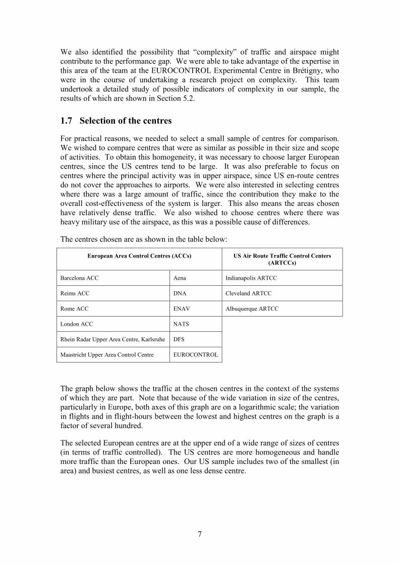
The graph below shows the traffic at the chosen centres in the context of the systemsof which they are part. Note that because of the wide variation in size of the centres,particularly in Europe, both axes of this graph are on a logarithmic scale; the variationin flights and in flight-hours between the lowest and highest centres on the graph is afactor of several hundred.

The selected European centres are at the upper end of a wide range of sizes of centres(in terms of traffic controlled). The US centres are more homogeneous and handlemore traffic than the European ones. Our US sample includes two of the smallest (inarea) and busiest centres, as well as one less dense centre.

8

Figure 1.3: Traffic handled by US and European centres, 2001

10 000

100 000

1 000 000

10 000 000

10 000 100 000 1 000 000 10 000 000

Area controlled in sq km(log scale)

Flights in 2001

(log scale)

EuropeUSEuropean sampleUS sample

Barcelona

Reims

Karlsruhe

Roma

Maastricht

London

Albuquerque

Indianapolis

Cleveland

European average

US average

The size of the selected sample is put in the context of the size of the two systems in Figure1.4. The selected European centres accounted for 19% of the flight-hours handled in theairspace of EUROCONTROL Member States in 2001, and some 6% of the en-route cost.The US centres accounted for some 12% of the flight-hours handled in the ARTCCs in theyear to September 2001, and 7% of the en-route cost.

Figure 1.4: The size of our sample in the context of the two systems

0%

5%

10%

15%

20%

Flight hours Area controlled(sq km)

Sectors ATCOs Total staff En-route costs

% European sample% US sample

In Chapter 2 we describe the centres selected.

9

2 Description of selected centres

2.1 Introduction

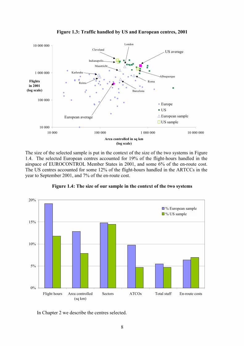
The map in Figure 2.1 indicates the location of the centres in the sample.

Figure 2.1: Location of airspace of selected centres

In the following paragraphs we present first a comparison of key features of thecentre, followed by a brief description of each one. More details on the centres can befound in the fact sheets provided as Annex A to this paper, and certain aspects of thetraffic characteristics of each centre are described in Chapter 5.

2.2 Comparison of key features

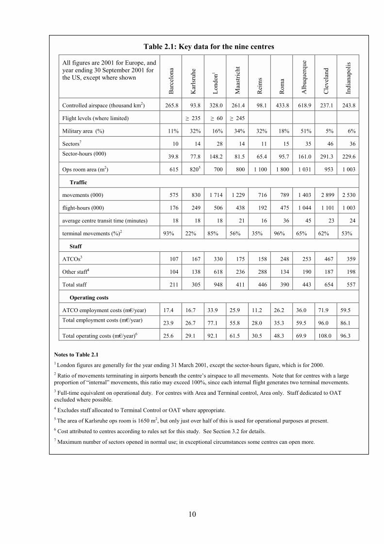
Table 2.1 summarises key features of the centres chosen.

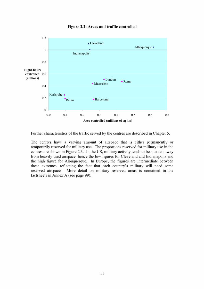
The centres were chosen to be relatively busy, and to be of comparable size.Figure 2.2 below (see page 11) demonstrates the area of airspace handled (the figuresinclude reserved military areas, where applicable) and the traffic, in terms of flight-hours controlled. In the European centres, there is a clear correlation between flight-hours and area controlled; this implies that they are all comparably busy centres. Inthe US, Albuquerque, though substantially bigger in area, is comparably busy.Cleveland and Indianapolis, by contrast, while much the same area as the Europeancentres, handle much more traffic.

10

Table 2.1: Key data for the nine centres

All figures are 2001 for Europe, andyear ending 30 September 2001 forthe US, except where shown

Bar

celo

na

Kar

lsru

he

Lond

on1

Maa

stric

ht

Rei

ms

Rom

a

Alb

uque

rque

Cle

vela

nd

Indi

anap

olis

Controlled airspace (thousand km2) 265.8 93.8 328.0 261.4 98.1 433.8 618.9 237.1 243.8

Flight levels (where limited) ≥ 235 ≥ 60 ≥ 245

Military area (%) 11% 32% 16% 34% 32% 18% 51% 5% 6%

Sectors7 10 14 28 14 11 15 35 46 36

Sector-hours (000) 39.8 77.8 148.2 81.5 65.4 95.7 161.0 291.3 229.6

Ops room area (m2) 615 8205 700 800 1 100 1 800 1 031 953 1 003

Traffic

movements (000) 575 830 1 714 1 229 716 789 1 403 2 899 2 530

flight-hours (000) 176 249 506 438 192 475 1 044 1 101 1 003

average centre transit time (minutes) 18 18 18 21 16 36 45 23 24

terminal movements (%)2 93% 22% 85% 56% 35% 96% 65% 62% 53%

Staff

ATCOs3 107 167 330 175 158 248 253 467 359

Other staff4 104 138 618 236 288 134 190 187 198

Total staff 211 305 948 411 446 390 443 654 557

Operating costs

ATCO employment costs (m�/year) 17.4 16.7 33.9 25.9 11.2 26.2 36.0 71.9 59.5

Total employment costs (m�/year) 23.9 26.7 77.1 55.8 28.0 35.3 59.5 96.0 86.1

Total operating costs (m�/year)6 25.6 29.1 92.1 61.5 30.5 48.3 69.9 108.0 96.3

Notes to Table 2.11 London figures are generally for the year ending 31 March 2001, except the sector-hours figure, which is for 2000.2 Ratio of movements terminating in airports beneath the centre�s airspace to all movements. Note that for centres with a largeproportion of �internal� movements, this ratio may exceed 100%, since each internal flight generates two terminal movements.3 Full-time equivalent on operational duty. For centres with Area and Terminal control, Area only. Staff dedicated to OATexcluded where possible.4 Excludes staff allocated to Terminal Control or OAT where appropriate.5 The area of Karlsruhe ops room is 1650 m2, but only just over half of this is used for operational purposes at present.6 Cost attributed to centres according to rules set for this study. See Section 3.2 for details.7 Maximum number of sectors opened in normal use; in exceptional circumstances some centres can open more.

11

Figure 2.2: Areas and traffic controlled

Albuquerque

Indianapolis

Cleveland

Karlsruhe

Reims Barcelona

MaastrichtLondon Roma

0

0.2

0.4

0.6

0.8

1

1.2

0.0 0.1 0.2 0.3 0.4 0.5 0.6 0.7

Area controlled (millions of sq km)

Flight-hourscontrolled(millions)

Further characteristics of the traffic served by the centres are described in Chapter 5.

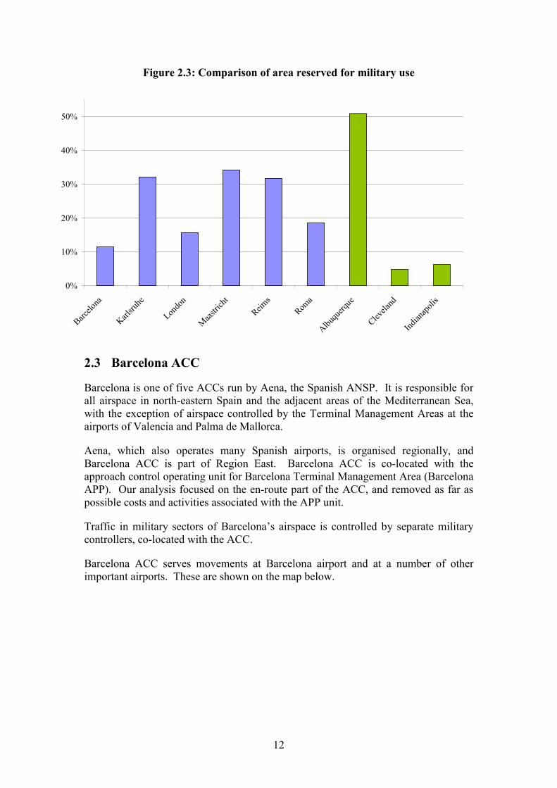
The centres have a varying amount of airspace that is either permanently ortemporarily reserved for military use. The proportions reserved for military use in thecentres are shown in Figure 2.3. In the US, military activity tends to be situated awayfrom heavily used airspace: hence the low figures for Cleveland and Indianapolis andthe high figure for Albuquerque. In Europe, the figures are intermediate betweenthese extremes, reflecting the fact that each country�s military will need somereserved airspace. More detail on military reserved areas is contained in thefactsheets in Annex A (see page 99).

12

Figure 2.3: Comparison of area reserved for military use

0%

10%

20%

30%

40%

50%

Barcelo

na

Karlsru

he

Londo

n

Maastric

htReim

sRom

a

Albuqu

erque

Clevela

nd

Indian

apoli

s

2.3 Barcelona ACC

Barcelona is one of five ACCs run by Aena, the Spanish ANSP. It is responsible forall airspace in north-eastern Spain and the adjacent areas of the Mediterranean Sea,with the exception of airspace controlled by the Terminal Management Areas at theairports of Valencia and Palma de Mallorca.

Aena, which also operates many Spanish airports, is organised regionally, andBarcelona ACC is part of Region East. Barcelona ACC is co-located with theapproach control operating unit for Barcelona Terminal Management Area (BarcelonaAPP). Our analysis focused on the en-route part of the ACC, and removed as far aspossible costs and activities associated with the APP unit.

Traffic in military sectors of Barcelona�s airspace is controlled by separate militarycontrollers, co-located with the ACC.

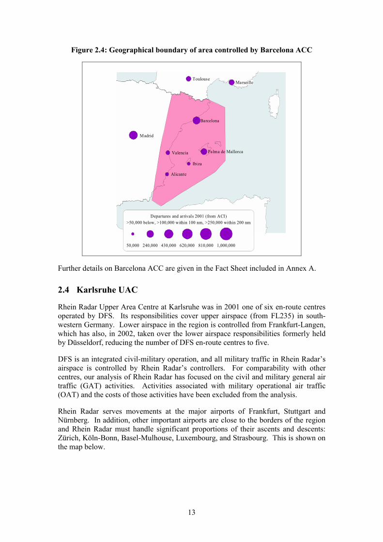
Barcelona ACC serves movements at Barcelona airport and at a number of otherimportant airports. These are shown on the map below.

13

Figure 2.4: Geographical boundary of area controlled by Barcelona ACC

Alicante

Barcelona

Ibiza

Palma de MallorcaValencia

Madrid

MarseilleToulouse

Departures and arrivals 2001 (from ACI)>50,000 below, >100,000 within 100 nm, >250,000 within 200 nm

50,000 240,000 430,000 620,000 810,000 1,000,000

Further details on Barcelona ACC are given in the Fact Sheet included in Annex A.

2.4 Karlsruhe UAC

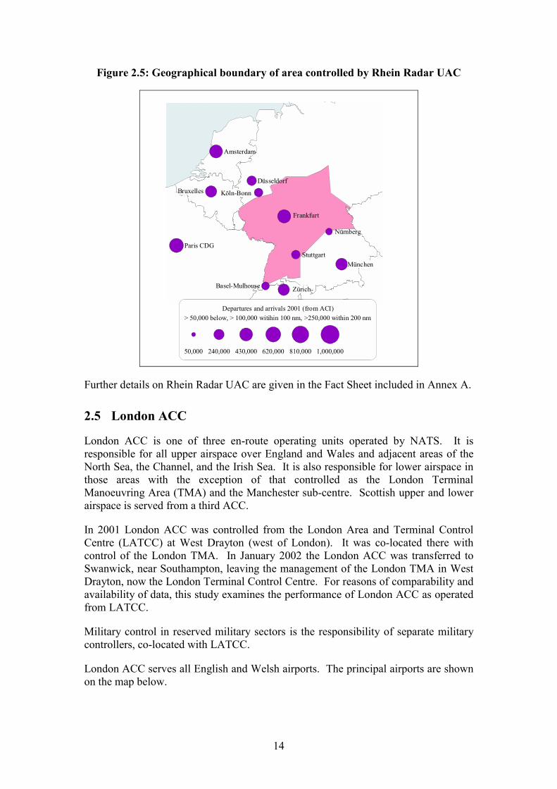
Rhein Radar Upper Area Centre at Karlsruhe was in 2001 one of six en-route centresoperated by DFS. Its responsibilities cover upper airspace (from FL235) in south-western Germany. Lower airspace in the region is controlled from Frankfurt-Langen,which has also, in 2002, taken over the lower airspace responsibilities formerly heldby Düsseldorf, reducing the number of DFS en-route centres to five.

DFS is an integrated civil-military operation, and all military traffic in Rhein Radar�sairspace is controlled by Rhein Radar�s controllers. For comparability with othercentres, our analysis of Rhein Radar has focused on the civil and military general airtraffic (GAT) activities. Activities associated with military operational air traffic(OAT) and the costs of those activities have been excluded from the analysis.

Rhein Radar serves movements at the major airports of Frankfurt, Stuttgart andNürnberg. In addition, other important airports are close to the borders of the regionand Rhein Radar must handle significant proportions of their ascents and descents:Zürich, Köln-Bonn, Basel-Mulhouse, Luxembourg, and Strasbourg. This is shown onthe map below.

14

Figure 2.5: Geographical boundary of area controlled by Rhein Radar UAC

Frankfurt

Nürnberg

Stuttgart

Amsterdam

München

Paris CDG

Zürich

Bruxelles

Basel-Mulhouse

Düsseldorf

Köln-Bonn

Departures and arrivals 2001 (from ACI)> 50,000 below, > 100,000 witihin 100 nm, >250,000 within 200 nm

50,000 240,000 430,000 620,000 810,000 1,000,000

Further details on Rhein Radar UAC are given in the Fact Sheet included in Annex A.

2.5 London ACC

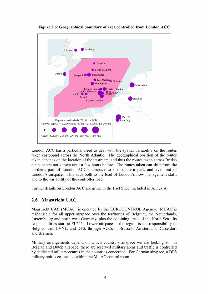
London ACC is one of three en-route operating units operated by NATS. It isresponsible for all upper airspace over England and Wales and adjacent areas of theNorth Sea, the Channel, and the Irish Sea. It is also responsible for lower airspace inthose areas with the exception of that controlled as the London TerminalManoeuvring Area (TMA) and the Manchester sub-centre. Scottish upper and lowerairspace is served from a third ACC.

In 2001 London ACC was controlled from the London Area and Terminal ControlCentre (LATCC) at West Drayton (west of London). It was co-located there withcontrol of the London TMA. In January 2002 the London ACC was transferred toSwanwick, near Southampton, leaving the management of the London TMA in WestDrayton, now the London Terminal Control Centre. For reasons of comparability andavailability of data, this study examines the performance of London ACC as operatedfrom LATCC.

Military control in reserved military sectors is the responsibility of separate militarycontrollers, co-located with LATCC.

London ACC serves all English and Welsh airports. The principal airports are shownon the map below.

15

Figure 2.6: Geographical boundary of area controlled from London ACC

Birmingham

BristolCardiff

East Midlands

Leeds-Bradford

Liverpool

London City

London Gatwick

London HeathrowLondon Luton London Stansted

Manchester

Norwich

Southend

Teesside

Dublin

EdinburghGlasgow

Paris Orly

Amsterdam

Paris CDG

Bruxelles

Departures and arrivals 2001 (from ACI)> 50,000 below, > 100,000 within 100 nm, > 250,000 within 200 nm

50,000 240,000 430,000 620,000 810,000 1,000,000

London ACC has a particular need to deal with the spatial variability on the routestaken eastbound across the North Atlantic. The geographical position of the routestaken depends on the location of the jetstream, and thus the routes taken across Britishairspace are not known until a few hours before. The routes taken can shift from thenorthern part of London ACC�s airspace to the southern part, and even out ofLondon�s airspace. This adds both to the load of London�s flow management staff,and to the variability of the controller load.

Further details on London ACC are given in the Fact Sheet included in Annex A.

2.6 Maastricht UAC

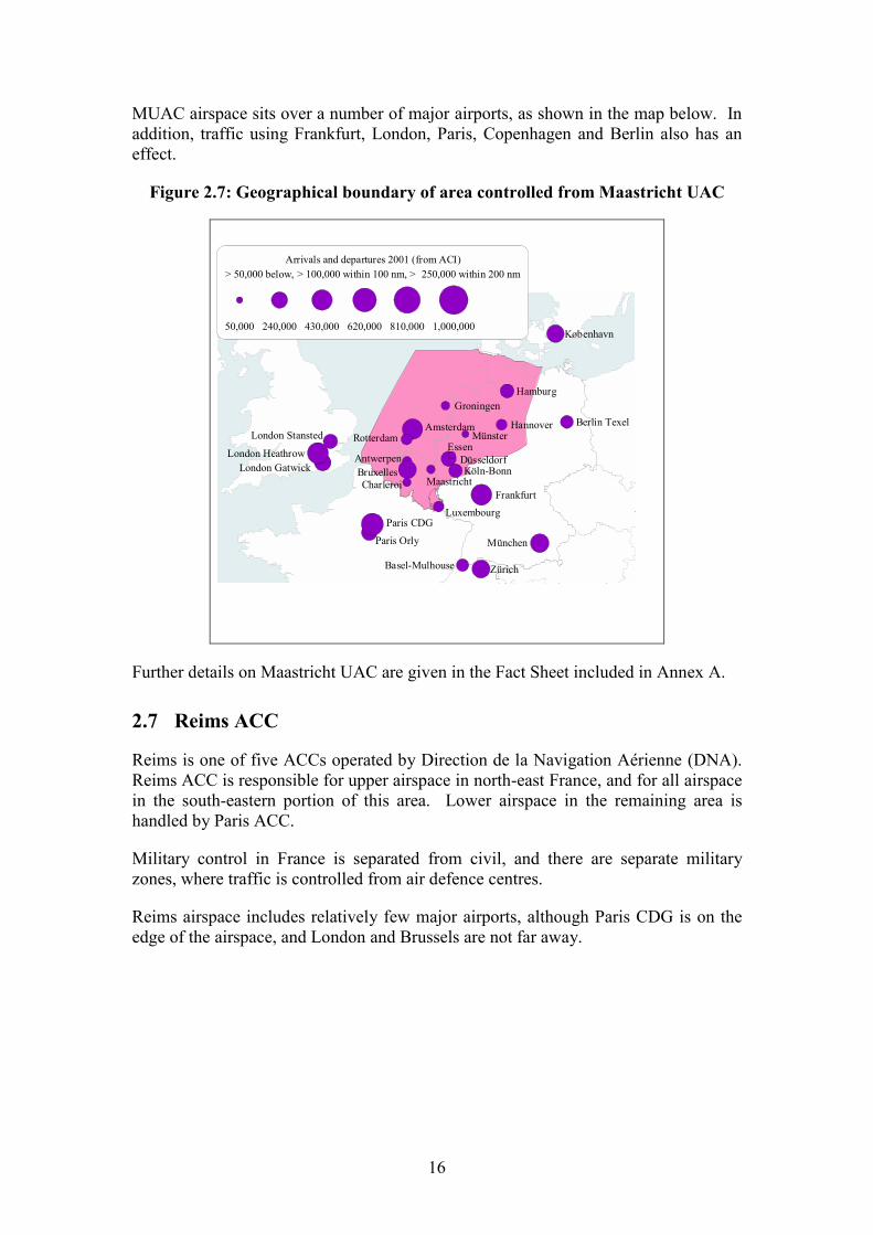
Maastricht UAC (MUAC) is operated by the EUROCONTROL Agency. MUAC isresponsible for all upper airspace over the territories of Belgium, the Netherlands,Luxembourg and north-west Germany, plus the adjoining areas of the North Sea. Itsresponsibilities start at FL245. Lower airspace in the region is the responsibility ofBelgocontrol, LVNL, and DFS, through ACCs in Brussels, Amsterdam, Düsseldorfand Bremen.

Military arrangements depend on which country�s airspace we are looking at. InBelgian and Dutch airspace, there are reserved military areas and traffic is controlledby dedicated military centres in the countries concerned. For German airspace, a DFSmilitary unit is co-located within the MUAC control room.

16

MUAC airspace sits over a number of major airports, as shown in the map below. Inaddition, traffic using Frankfurt, London, Paris, Copenhagen and Berlin also has aneffect.

Figure 2.7: Geographical boundary of area controlled from Maastricht UAC

Amsterdam

Basel-Mulhouse

Berlin Texel

København

London Gatwick

London Stansted

Paris Orly

AntwerpenBruxellesCharleroi

DüsseldorfEssen

GroningenHamburg

Hannover

Köln-Bonn

Luxembourg

Maastricht

MünsterRotterdam

Frankfurt

London Heathrow

München

Paris CDG

Zürich

Arrivals and departures 2001 (from ACI)> 50,000 below, > 100,000 within 100 nm, > 250,000 within 200 nm

50,000 240,000 430,000 620,000 810,000 1,000,000

Further details on Maastricht UAC are given in the Fact Sheet included in Annex A.

2.7 Reims ACC

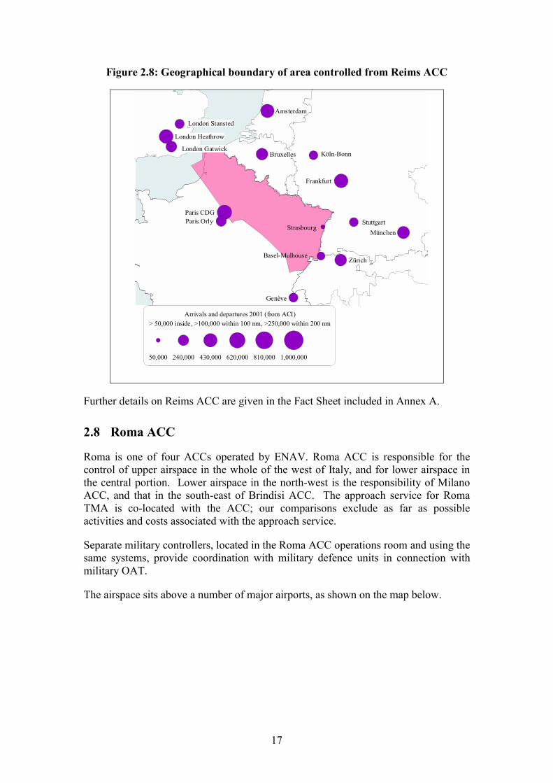
Reims is one of five ACCs operated by Direction de la Navigation Aérienne (DNA).Reims ACC is responsible for upper airspace in north-east France, and for all airspacein the south-eastern portion of this area. Lower airspace in the remaining area ishandled by Paris ACC.

Military control in France is separated from civil, and there are separate militaryzones, where traffic is controlled from air defence centres.

Reims airspace includes relatively few major airports, although Paris CDG is on theedge of the airspace, and London and Brussels are not far away.

17

Figure 2.8: Geographical boundary of area controlled from Reims ACC

Paris CDG

Strasbourg

Amsterdam

London Heathrow

München

Zürich

Bruxelles

Frankfurt

Basel-Mulhouse

Genève

Köln-BonnLondon Gatwick

London Stansted

Paris Orly Stuttgart

Arrivals and departures 2001 (from ACI)> 50,000 inside, >100,000 within 100 nm, >250,000 within 200 nm

50,000 240,000 430,000 620,000 810,000 1,000,000

Further details on Reims ACC are given in the Fact Sheet included in Annex A.

2.8 Roma ACC

Roma is one of four ACCs operated by ENAV. Roma ACC is responsible for thecontrol of upper airspace in the whole of the west of Italy, and for lower airspace inthe central portion. Lower airspace in the north-west is the responsibility of MilanoACC, and that in the south-east of Brindisi ACC. The approach service for RomaTMA is co-located with the ACC; our comparisons exclude as far as possibleactivities and costs associated with the approach service.

Separate military controllers, located in the Roma ACC operations room and using thesame systems, provide coordination with military defence units in connection withmilitary OAT.

The airspace sits above a number of major airports, as shown on the map below.

18

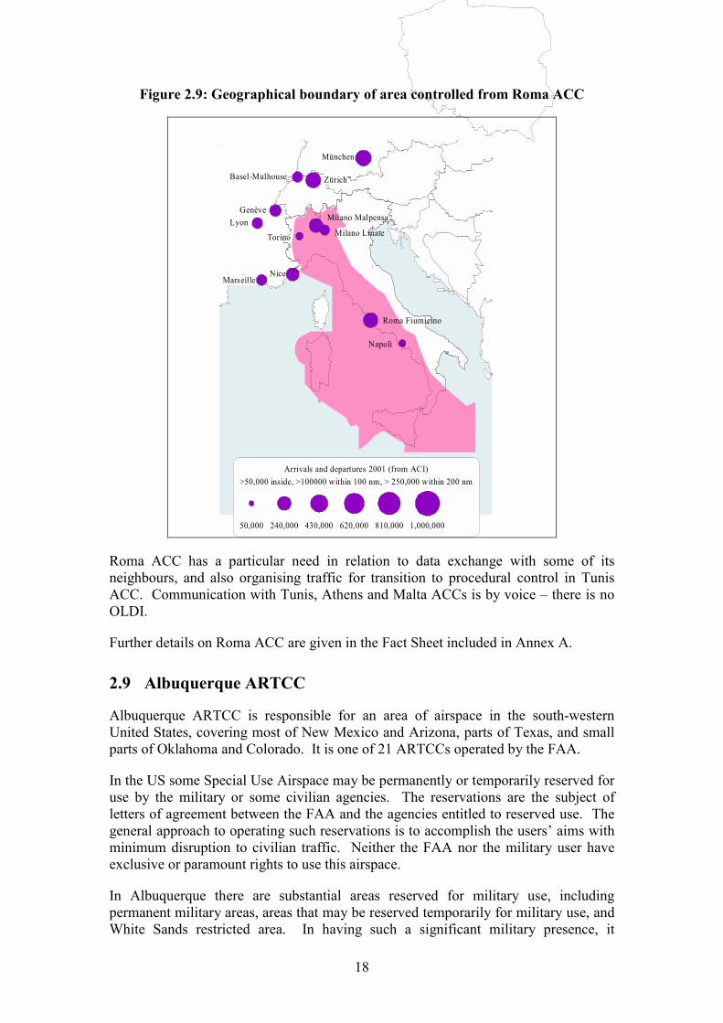
Figure 2.9: Geographical boundary of area controlled from Roma ACC

Milano Linate

Milano Malpensa

Napoli

Roma Fiumicino

Torino

München

ZürichBasel-Mulhouse

GenèveLyon

MarseilleNice

Arrivals and departures 2001 (from ACI)>50,000 inside, >100000 within 100 nm, > 250,000 within 200 nm

50,000 240,000 430,000 620,000 810,000 1,000,000

Roma ACC has a particular need in relation to data exchange with some of itsneighbours, and also organising traffic for transition to procedural control in TunisACC. Communication with Tunis, Athens and Malta ACCs is by voice � there is noOLDI.

Further details on Roma ACC are given in the Fact Sheet included in Annex A.

2.9 Albuquerque ARTCC

Albuquerque ARTCC is responsible for an area of airspace in the south-westernUnited States, covering most of New Mexico and Arizona, parts of Texas, and smallparts of Oklahoma and Colorado. It is one of 21 ARTCCs operated by the FAA.

In the US some Special Use Airspace may be permanently or temporarily reserved foruse by the military or some civilian agencies. The reservations are the subject ofletters of agreement between the FAA and the agencies entitled to reserved use. Thegeneral approach to operating such reservations is to accomplish the users� aims withminimum disruption to civilian traffic. Neither the FAA nor the military user haveexclusive or paramount rights to use this airspace.

In Albuquerque there are substantial areas reserved for military use, includingpermanent military areas, areas that may be reserved temporarily for military use, andWhite Sands restricted area. In having such a significant military presence, it

19

resembles some of the European centres we are examining. The influence ofsignificant military areas and how it differs between Europe and the US is examinedin Section 10.3.

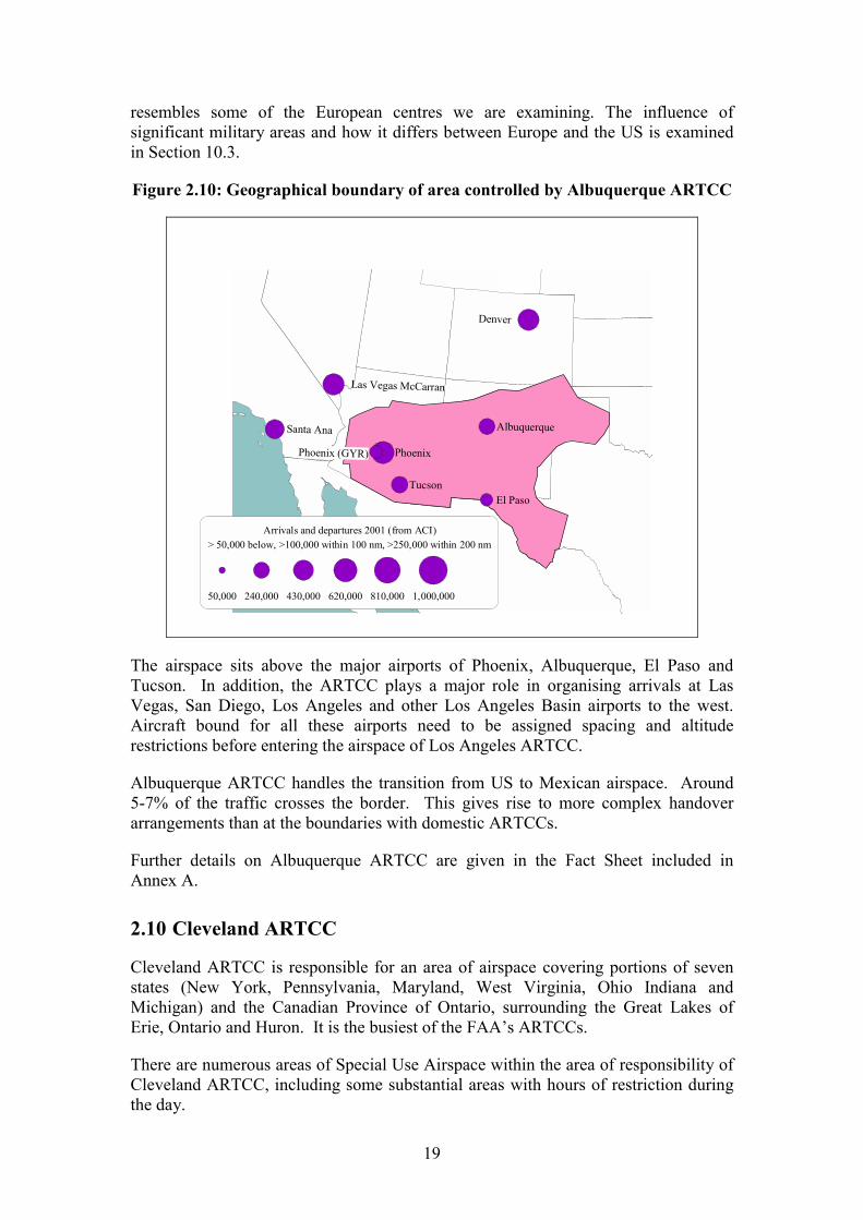
Figure 2.10: Geographical boundary of area controlled by Albuquerque ARTCC

Albuquerque

El Paso

PhoenixPhoenix (GYR)

Tucson

Denver

Las Vegas McCarran

Santa Ana

Arrivals and departures 2001 (from ACI)> 50,000 below, >100,000 within 100 nm, >250,000 within 200 nm

50,000 240,000 430,000 620,000 810,000 1,000,000

The airspace sits above the major airports of Phoenix, Albuquerque, El Paso andTucson. In addition, the ARTCC plays a major role in organising arrivals at LasVegas, San Diego, Los Angeles and other Los Angeles Basin airports to the west.Aircraft bound for all these airports need to be assigned spacing and altituderestrictions before entering the airspace of Los Angeles ARTCC.

Albuquerque ARTCC handles the transition from US to Mexican airspace. Around5-7% of the traffic crosses the border. This gives rise to more complex handoverarrangements than at the boundaries with domestic ARTCCs.

Further details on Albuquerque ARTCC are given in the Fact Sheet included inAnnex A.

2.10 Cleveland ARTCC

Cleveland ARTCC is responsible for an area of airspace covering portions of sevenstates (New York, Pennsylvania, Maryland, West Virginia, Ohio Indiana andMichigan) and the Canadian Province of Ontario, surrounding the Great Lakes ofErie, Ontario and Huron. It is the busiest of the FAA�s ARTCCs.

There are numerous areas of Special Use Airspace within the area of responsibility ofCleveland ARTCC, including some substantial areas with hours of restriction duringthe day.

20

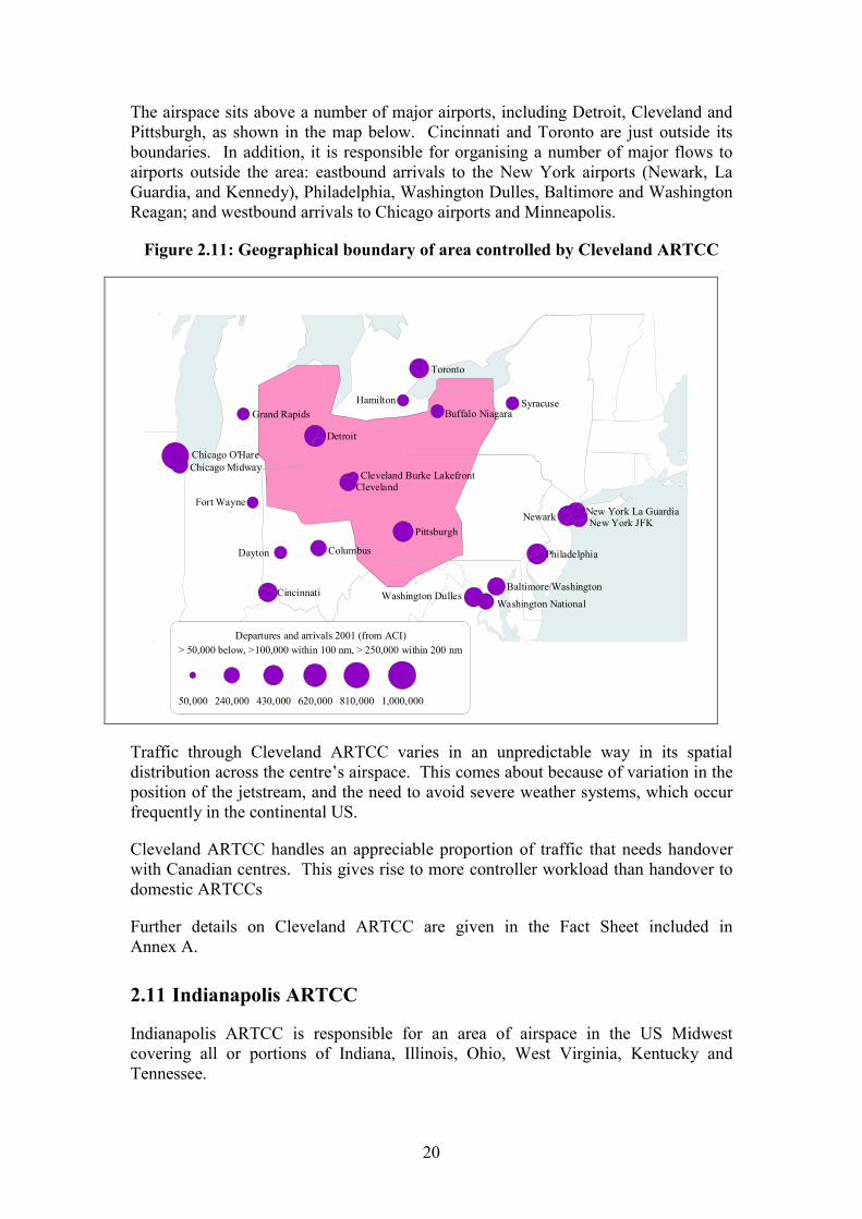
The airspace sits above a number of major airports, including Detroit, Cleveland andPittsburgh, as shown in the map below. Cincinnati and Toronto are just outside itsboundaries. In addition, it is responsible for organising a number of major flows toairports outside the area: eastbound arrivals to the New York airports (Newark, LaGuardia, and Kennedy), Philadelphia, Washington Dulles, Baltimore and WashingtonReagan; and westbound arrivals to Chicago airports and Minneapolis.

Figure 2.11: Geographical boundary of area controlled by Cleveland ARTCC

Buffalo Niagara

ClevelandCleveland Burke Lakefront

Cincinnati

Detroit

Hamilton

Pittsburgh

New York La GuardiaNewark

Philadelphia

Toronto

Washington Dulles

Chicago O'Hare

ColumbusDayton

Fort Wayne

Grand RapidsSyracuse

Washington National

Baltimore/Washington

Chicago Midway

New York JFK

Departures and arrivals 2001 (from ACI)> 50,000 below, >100,000 within 100 nm, > 250,000 within 200 nm

50,000 240,000 430,000 620,000 810,000 1,000,000

Traffic through Cleveland ARTCC varies in an unpredictable way in its spatialdistribution across the centre�s airspace. This comes about because of variation in theposition of the jetstream, and the need to avoid severe weather systems, which occurfrequently in the continental US.

Cleveland ARTCC handles an appreciable proportion of traffic that needs handoverwith Canadian centres. This gives rise to more controller workload than handover todomestic ARTCCs

Further details on Cleveland ARTCC are given in the Fact Sheet included inAnnex A.

2.11 Indianapolis ARTCC

Indianapolis ARTCC is responsible for an area of airspace in the US Midwestcovering all or portions of Indiana, Illinois, Ohio, West Virginia, Kentucky andTennessee.

21

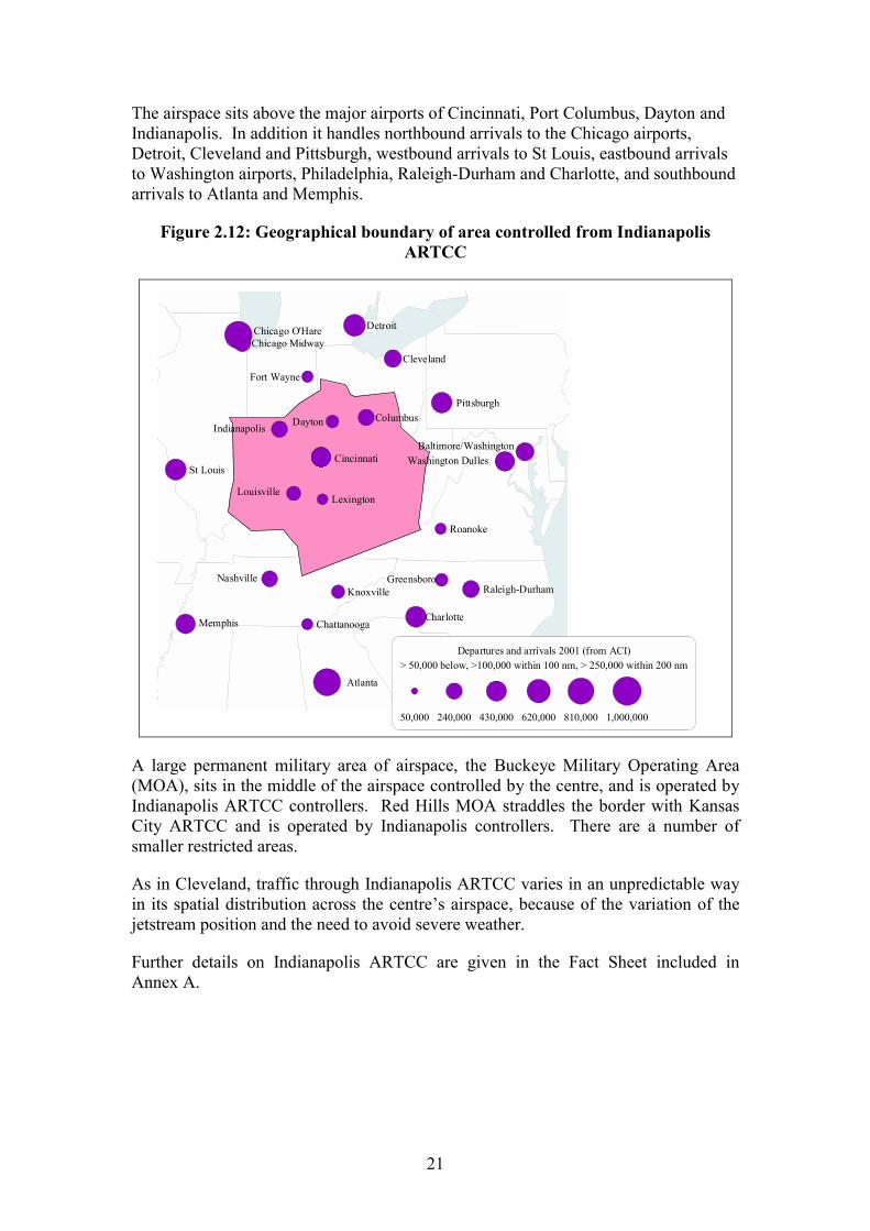
The airspace sits above the major airports of Cincinnati, Port Columbus, Dayton andIndianapolis. In addition it handles northbound arrivals to the Chicago airports,Detroit, Cleveland and Pittsburgh, westbound arrivals to St Louis, eastbound arrivalsto Washington airports, Philadelphia, Raleigh-Durham and Charlotte, and southboundarrivals to Atlanta and Memphis.

Figure 2.12: Geographical boundary of area controlled from IndianapolisARTCC

Cincinnati

ColumbusDaytonIndianapolis

LouisvilleLexington

Atlanta

Baltimore/Washington

Charlotte

Chicago O'Hare Detroit

Memphis

Pittsburgh

St Louis

Chattanooga

Cleveland

Fort Wayne

GreensboroKnoxville

Nashville

Roanoke

Chicago Midway

Washington Dulles

Raleigh-Durham

Departures and arrivals 2001 (from ACI)> 50,000 below, >100,000 within 100 nm, > 250,000 within 200 nm

50,000 240,000 430,000 620,000 810,000 1,000,000

A large permanent military area of airspace, the Buckeye Military Operating Area(MOA), sits in the middle of the airspace controlled by the centre, and is operated byIndianapolis ARTCC controllers. Red Hills MOA straddles the border with KansasCity ARTCC and is operated by Indianapolis controllers. There are a number ofsmaller restricted areas.

As in Cleveland, traffic through Indianapolis ARTCC varies in an unpredictable wayin its spatial distribution across the centre�s airspace, because of the variation of thejetstream position and the need to avoid severe weather.

Further details on Indianapolis ARTCC are given in the Fact Sheet included inAnnex A.

22

23

3 How we are comparing performance

3.1 Introduction

In this study, we are comparing cost-effectiveness in centres by defining the output ofthe centre, and comparing the ratio of that output to defined inputs, such as costs. Wethen break down this ratio into a number of component ratios, to examine in moredetail how the aggregate performance differences arise. In this section we discuss themeasures of output and input that we have used, and the way we have broken downthe overall cost-effectiveness ratio.

It is important in comparing centres:

• to ensure that the comparison takes into account the fact that different centresperform different sets of activities, particularly in the division of activitiesbetween centres and the ANSP HQ;

• to understand the uncontrollable factors that give rise to differences inperformance indicators that do not necessarily reflect differences in underlyingperformance.

In the next sub-section, we discuss the quantitative analysis that we are undertakingfor the purpose of cost-effectiveness comparison. The work draws heavily on theframework developed by the PRU for previous comparisons of performance acrossEurope. However, the framework has been modified to reflect the fact that we arecomparing performance across centres, and enhanced to reflect the insights that thestudy has given us into the components of performance.

3.2 Outputs, inputs and overall cost-effectiveness

The definition of output

Clearly, the definition of what the output of a centre is, and how to measure it, arefundamental questions in performance comparison. For the purposes of this study, wehave adopted en-route flight-hours controlled as our main output indicator. Unlikekm controlled, this measure is readily available in both systems.

It could be argued that flight-hours should be adjusted to reflect airborne delay. It isdifficult, however, to measure airborne delay on either side of the Atlantic. For thisreason, we have not considered this further, and have assumed that flight-hours are avalid measure of output at centre level.

The definition of inputs

The resources that are used to provide the services comprise:

• labour � the staff who provide the services;

• capital � the assets used to produce them; and

24

• other resources, such as outsourced maintenance and utility costs.

In practice, distinguishing and separately analysing labour and non-labour resources isboth difficult � in that data are not readily available at a centre level � and notnecessarily informative, since:

(a) the balance between staff costs, as a whole, and other operating costs, isdetermined by the ANSP�s practices � in particular whether major items ofcosts are contracted out or staffed in-house; and

(b) the scope of services provided by a centre as opposed to its HQ cansignificantly vary from one ANSP to another.

To determine comparable costs for the centres (ACCs and ARTCCs) we need todefine closely which elements should be attributed to the centre. Our approach, basedon data availability and the lessons learnt from other studies, as well as theconsiderations of the Working Group, is to attribute a set of included operating coststo each centre. These comprise the direct costs incurred by providing air navigationservices from the centre, including the front-line staff and those required to supportthem directly, and the costs of providing and maintaining the operational systems atthe centre. A certain number of services are excluded, because in some cases they areprovided, or costs held, centrally. These comprise ancillary services such as MET,SAR, and AIS. Some activities are excluded because of their non-local nature:providing and maintaining the CNS infrastructure, R&D not specific to the centre, andthe ab initio training of controllers. General administrative costs (finance, humanresources, and similar cost categories), where dedicated to the centre, rather than tomore general activities of the ANSP, are included. No allocated HQ costs areincluded. Where a centre undertakes both terminal and area control, we have, forcomparability, excluded the ATCOs working on terminal control, and a portion of theother costs allocated to terminal control (based on the number of ATCOs).

The costs of capital and assets are also difficult to attribute to centres, particularly inthe US. For this reason we have in this study looked only at operating costs.

We have further divided operating costs into:

• the employment costs relating to ATCOs in OPS;

• other costs, comprising:

� the employment costs relating to other staff attributed to the centreaccording to the criteria set out above;

� non-staff operating costs attributed to the centre according to thecriteria set out above.

The benchmarks for operational cost-effectiveness

The above measures of inputs and outputs lead us to the following measure ofoperational cost-effectiveness at centre level:

• operating costs per flight-hour controlled.

25

In subsequent sections we discuss a performance framework that helps us break downthe differences in cost-effectiveness and understand in detail how differences betweencentres have arisen.

3.3 The analytical framework

The breakdown of cost-effectiveness

The framework has been devised to help us examine cost-effectiveness at a moredetailed level, to determine where apparent differences in performance arise.

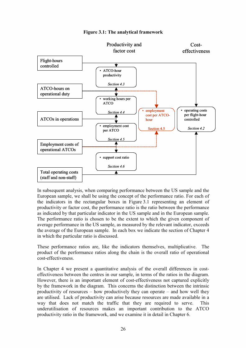
An internally self-consistent picture of the links between measures and performanceindicators is shown in Figure 3.1. In this diagram, each element in the rectangularboxes on the left-hand side is linked to adjacent ones by a ratio reflecting acontribution to cost-effectiveness. The overall operational cost-effectiveness � theoperating cost per flight-hour controlled - is the product of all these ratios. Thisframework has been developed pragmatically, taking account of what can be readilyand comparably measured.

The operational cost-effectiveness � the ratio shown on the extreme right of thediagram - comprises the product of four ratios, shown in the column to the left:

• ATCO-hour productivity � the number of flight-hours controlled for each hourspent by an ATCO on operational duty;

• the number of hours worked by those ATCOs;

• the employment costs of those ATCOs; and

• the support cost ratio � the total amount spent on staffing and running thecentre for each euro spent on employing ATCOs.

A particularly interesting combination of pairs of these ratios is also presented in thefigure:

• the employment cost per ATCO-hour (combining employment cost per ATCOand ATCO-hours).

26

Figure 3.1: The analytical framework


Section 4.2



ATCOs in operations



Cost-effectiveness


� working hours per ATCO

Section 4.4

� employment cost per ATCO

Section 4.5

� support cost ratio

Section 4.6


Section 4.3

� employment cost per ATCO-hour

Section 4.5


Section 4.2



ATCOs in operations



Cost-effectiveness


� working hours per ATCO

Section 4.4

� employment cost per ATCO

Section 4.5

� support cost ratio

Section 4.6


Section 4.3

� employment cost per ATCO-hour

Section 4.5

In subsequent analysis, when comparing performance between the US sample and theEuropean sample, we shall be using the concept of the performance ratio. For each ofthe indicators in the rectangular boxes in Figure 3.1 representing an element ofproductivity or factor cost, the performance ratio is the ratio between the performanceas indicated by that particular indicator in the US sample and in the European sample.The performance ratio is chosen to be the extent to which the given component ofaverage performance in the US sample, as measured by the relevant indicator, exceedsthe average of the European sample. In each box we indicate the section of Chapter 4in which the particular ratio is discussed.

These performance ratios are, like the indicators themselves, multiplicative. Theproduct of the performance ratios along the chain is the overall ratio of operationalcost-effectiveness.

In Chapter 4 we present a quantitative analysis of the overall differences in cost-effectiveness between the centres in our sample, in terms of the ratios in the diagram.However, there is an important element of cost-effectiveness not captured explicitlyby the framework in the diagram. This concerns the distinction between the intrinsicproductivity of resources � how productively they can operate � and how well theyare utilised. Lack of productivity can arise because resources are made available in away that does not match the traffic that they are required to serve. Thisunderutilisation of resources makes an important contribution to the ATCOproductivity ratio in the framework, and we examine it in detail in Chapter 6.

27

3.4 Data sources

We have drawn data from two main sources:

• PRU work on Information Disclosure, ACE 2000 and ACE 2001;

• information provided by the participating ANSPs concerning their centres � inparticular, details of operational practices, and performance data, and financialinformation in sufficient detail for us to make the attributions of costsdescribed in Section 3.2.

Unavoidably, the information relates to different time periods. The US fiscal year onwhich data are collected runs from October to September, and the latest year that wehave data for is the year to September 2001.

For the European centres, we have been able to collect data consistently for the year2001, with the exception of London. NATS has a financial year running from April toMarch, so the latest year for which data were available was the year to March 2001.We have presented the data for the years in which it was available (making sure thatthe year is consistent between inputs and outputs); we do not believe that adjustmentto reach comparability will add any value to the comparison. We have used exchangerates of $1 = � 1.1 and £1 = � 1.61, figures appropriate for 2000 and 2001.

28

29

4 Review of results

4.1 Introduction

In this section we use the framework described in Chapter 3 and illustrated inFigure 3.1 to display the quantitative comparison of performance indicators from thestudy. We first compare the overall operational cost-effectiveness, then discuss itsbreakdown into the following main components:

• ATCO-hour productivity (flight-hours controlled per ATCO-hour);

• average hours worked per ATCO;

• employment costs per ATCO; and

• support cost ratio (total operating costs per � spent on ATCO employmentcosts).

We also examine the combination of pairs of these ratios, which are of interest:

• the output per ATCO (combining ATCO-hour productivity and ATCO-hours);and,

• the employment cost per ATCO-hour (combining employment cost per ATCOand ATCO-hours).

In Chapter 6, we break down further the ATCO-hour productivity, showing how it isdetermined both by the intrinsic ATCO-hour productivity, and how well the ATCOsare deployed to match the traffic (resource utilisation). In Chapter 7, we discuss thefactors that might influence resource utilisation.

On each comparison graph, we display a performance ratio, as defined in the previoussection, indicating the extent to which the average performance, as measured by eachindicator, in the US sample exceeds that of the European sample5. The product of theperformance ratios along the chain in Figure 3.1 is the overall operational cost-effectiveness ratio. We also display a miniature replica of Figure 3.1 in the bottomright of each diagram to guide the reader around the framework.

4.2 Operational cost-effectiveness

We present the comparison by first comparing the overall operational cost-effectiveness, then examining the components of this ratio in progressively moredepth.

5 Average ratios have been computed for each of the systems by taking the aggregate numerator for the centresbeing averaged and dividing by the aggregate denominator.

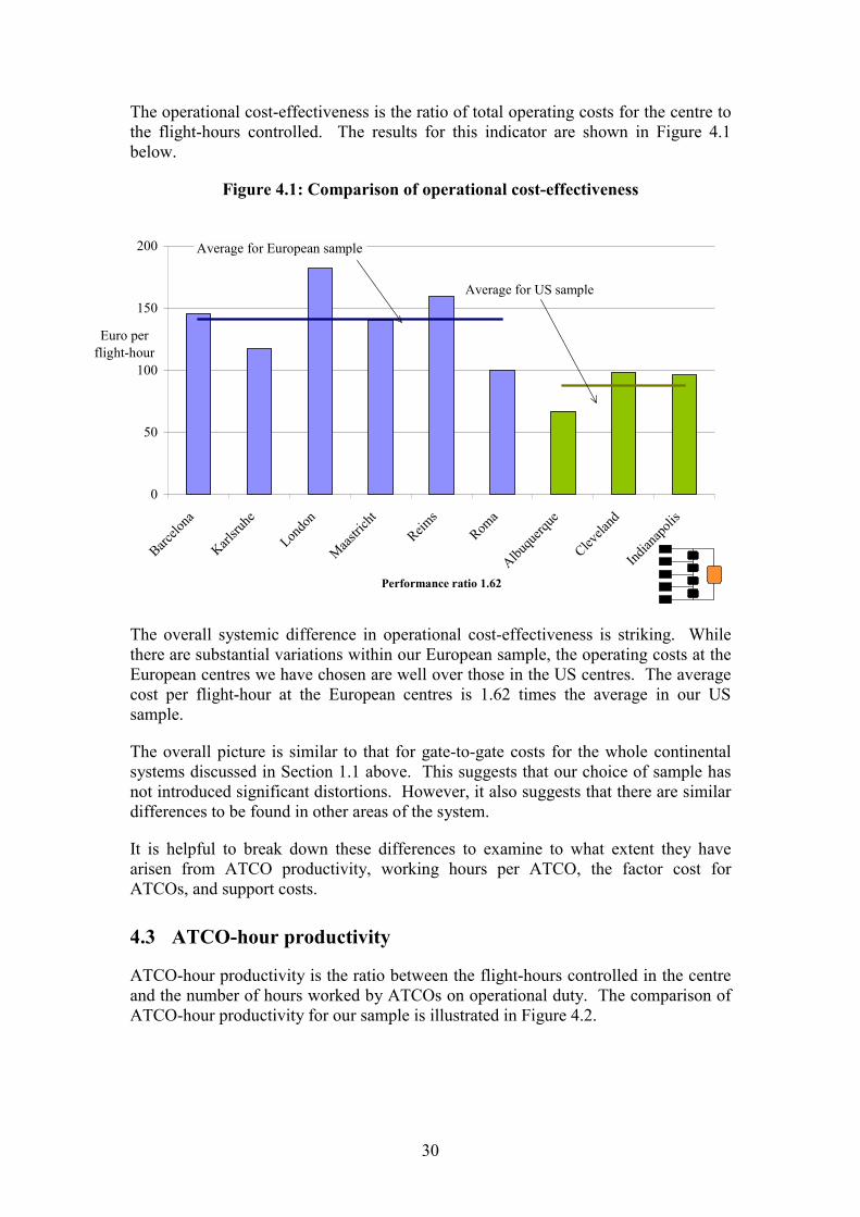
30

The operational cost-effectiveness is the ratio of total operating costs for the centre tothe flight-hours controlled. The results for this indicator are shown in Figure 4.1below.

Figure 4.1: Comparison of operational cost-effectiveness

0

50

100

150

200

Barcelo

na

Karlsru

he

Londo

n

Maastric

htReim

sRom

a

Albuqu

erque

Clevela

nd

Indian

apoli

s

Performance ratio 1.62

Euro per flight-hour

Average for European sample

Average for US sample

The overall systemic difference in operational cost-effectiveness is striking. Whilethere are substantial variations within our European sample, the operating costs at theEuropean centres we have chosen are well over those in the US centres. The averagecost per flight-hour at the European centres is 1.62 times the average in our USsample.

The overall picture is similar to that for gate-to-gate costs for the whole continentalsystems discussed in Section 1.1 above. This suggests that our choice of sample hasnot introduced significant distortions. However, it also suggests that there are similardifferences to be found in other areas of the system.

It is helpful to break down these differences to examine to what extent they havearisen from ATCO productivity, working hours per ATCO, the factor cost forATCOs, and support costs.

4.3 ATCO-hour productivity

ATCO-hour productivity is the ratio between the flight-hours controlled in the centreand the number of hours worked by ATCOs on operational duty. The comparison ofATCO-hour productivity for our sample is illustrated in Figure 4.2.

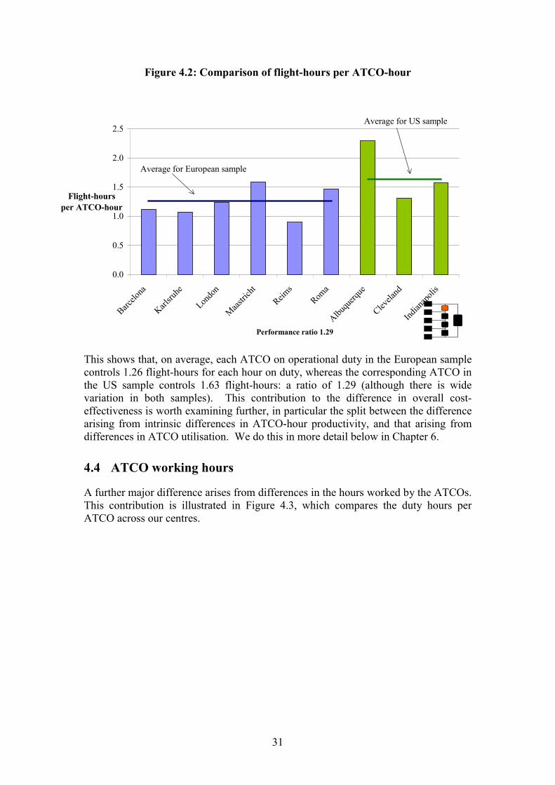
31

Figure 4.2: Comparison of flight-hours per ATCO-hour

0.0

0.5

1.0

1.5

2.0

2.5

Barcelo

na

Karlsru

he

Londo

n

Maastric

htReim

sRom

a

Albuqu

erque

Clevela

nd

Indian

apoli

s


Flight-hoursper ATCO-hour



This shows that, on average, each ATCO on operational duty in the European samplecontrols 1.26 flight-hours for each hour on duty, whereas the corresponding ATCO inthe US sample controls 1.63 flight-hours: a ratio of 1.29 (although there is widevariation in both samples). This contribution to the difference in overall cost-effectiveness is worth examining further, in particular the split between the differencearising from intrinsic differences in ATCO-hour productivity, and that arising fromdifferences in ATCO utilisation. We do this in more detail below in Chapter 6.

4.4 ATCO working hours

A further major difference arises from differences in the hours worked by the ATCOs.This contribution is illustrated in Figure 4.3, which compares the duty hours perATCO across our centres.

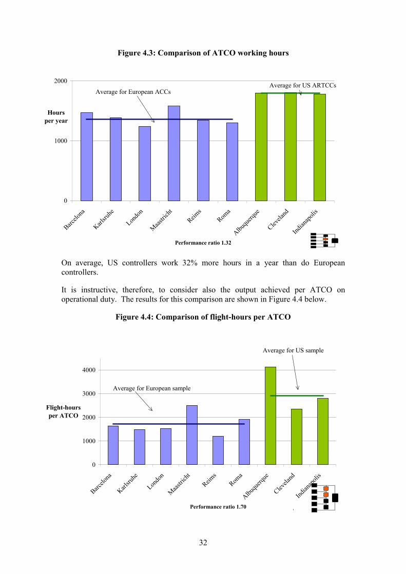
32

Figure 4.3: Comparison of ATCO working hours

0

1000

2000

Barcelo

na

Karlsru

he

Londo

n

Maastric

htReim

sRom

a

Albuqu

erque

Clevela

nd

Indian

apoli

s


Hours per year

Average for European ACCsAverage for US ARTCCs

On average, US controllers work 32% more hours in a year than do Europeancontrollers.

It is instructive, therefore, to consider also the output achieved per ATCO onoperational duty. The results for this comparison are shown in Figure 4.4 below.

Figure 4.4: Comparison of flight-hours per ATCO

0

1000

2000

3000

4000

Barcelo

na

Karlsru

he

Londo

n

Maastric

htReim

sRom

a

Albuqu

erque

Clevela

nd

Indian

apoli

s


Flight-hoursper ATCO



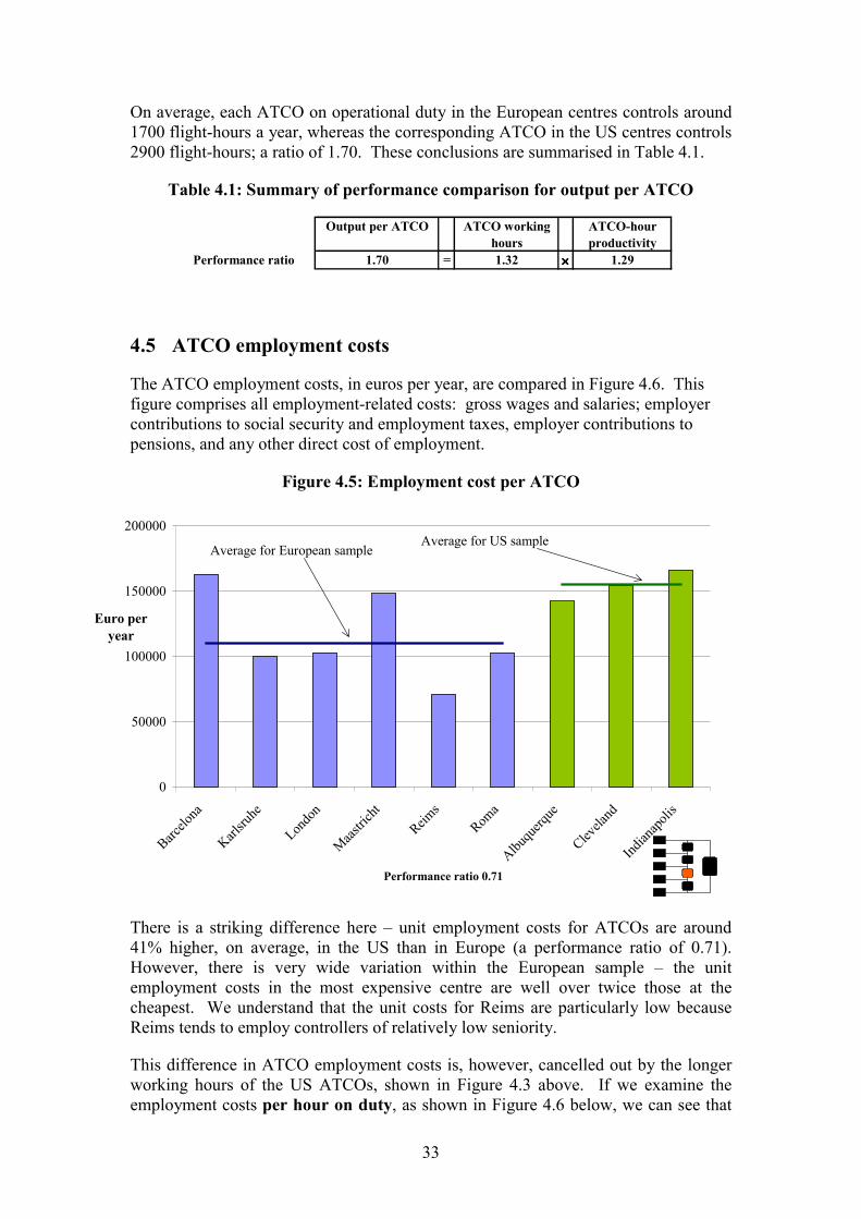
33

On average, each ATCO on operational duty in the European centres controls around1700 flight-hours a year, whereas the corresponding ATCO in the US centres controls2900 flight-hours; a ratio of 1.70. These conclusions are summarised in Table 4.1.

Table 4.1: Summary of performance comparison for output per ATCO

Output per ATCO ATCO working hours

ATCO-hour productivity

Performance ratio 1.70 = 1.32 ×××× 1.29

4.5 ATCO employment costs

The ATCO employment costs, in euros per year, are compared in Figure 4.6. Thisfigure comprises all employment-related costs: gross wages and salaries; employercontributions to social security and employment taxes, employer contributions topensions, and any other direct cost of employment.

Figure 4.5: Employment cost per ATCO

0

50000

100000

150000

200000

Barcelo

na

Karlsru

he

Londo

n

Maastric

htReim

sRom

a

Albuqu

erque

Clevela

nd

Indian

apoli

s


Euro peryear

Average for European sampleAverage for US sample

There is a striking difference here � unit employment costs for ATCOs are around41% higher, on average, in the US than in Europe (a performance ratio of 0.71).However, there is very wide variation within the European sample � the unitemployment costs in the most expensive centre are well over twice those at thecheapest. We understand that the unit costs for Reims are particularly low becauseReims tends to employ controllers of relatively low seniority.

This difference in ATCO employment costs is, however, cancelled out by the longerworking hours of the US ATCOs, shown in Figure 4.3 above. If we examine theemployment costs per hour on duty, as shown in Figure 4.6 below, we can see that

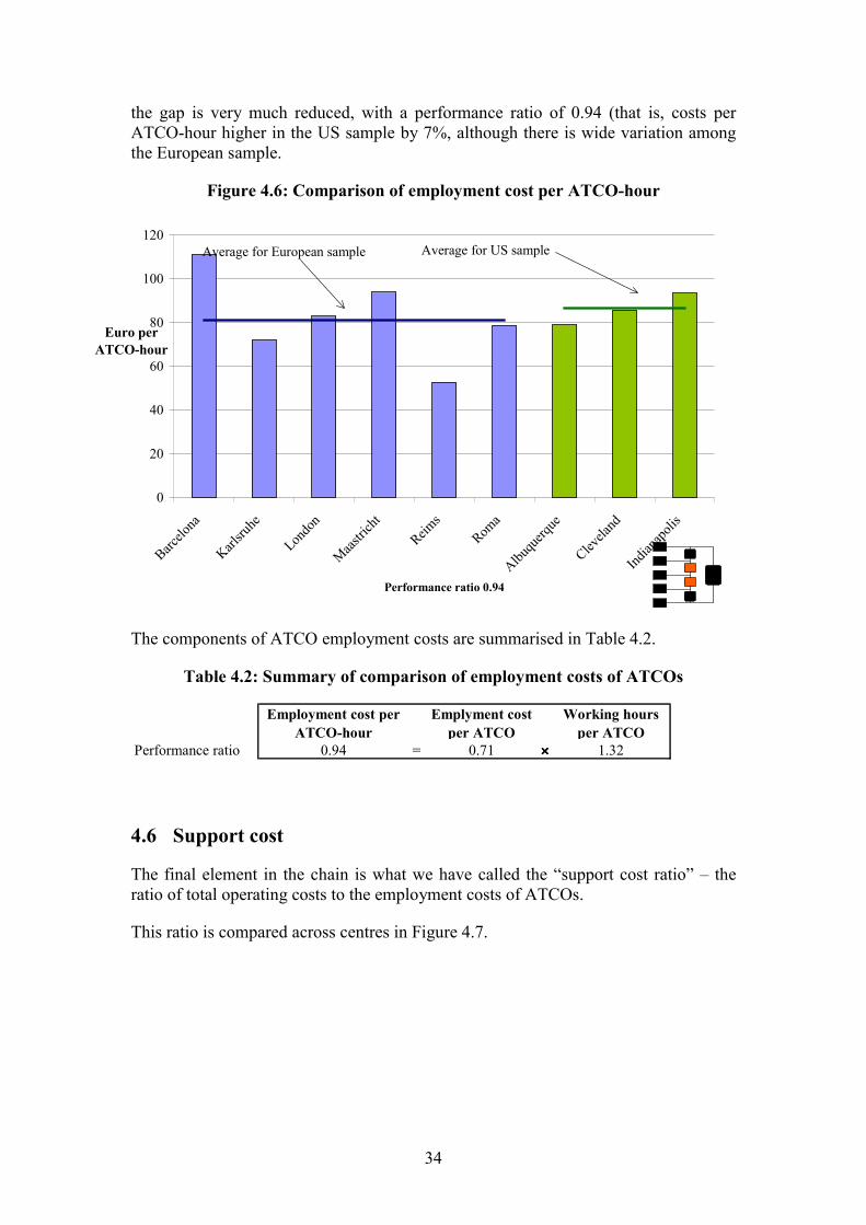
34

the gap is very much reduced, with a performance ratio of 0.94 (that is, costs perATCO-hour higher in the US sample by 7%, although there is wide variation amongthe European sample.

Figure 4.6: Comparison of employment cost per ATCO-hour

0

20

40

60

80

100

120

Barcelo

na

Karlsru

he

Londo

n

Maastric

htReim

sRom

a

Albuqu

erque

Clevela

nd

Indian

apoli

s


Euro perATCO-hour

Average for European sample Average for US sample

The components of ATCO employment costs are summarised in Table 4.2.

Table 4.2: Summary of comparison of employment costs of ATCOs

Employment cost per ATCO-hour

Emplyment cost per ATCO

Working hours per ATCO


4.6 Support cost

The final element in the chain is what we have called the �support cost ratio� � theratio of total operating costs to the employment costs of ATCOs.

This ratio is compared across centres in Figure 4.7.

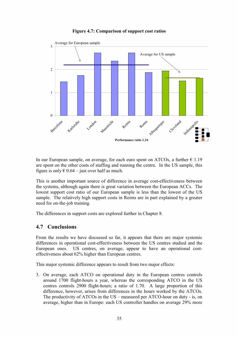
35

Figure 4.7: Comparison of support cost ratios

0

1

2

3

Barcelo

na

Karlsru

he

Londo

n

Maastric

htReim

sRom

a

Albuqu

erque

Clevela

nd

Indian

apoli

s




In our European sample, on average, for each euro spent on ATCOs, a further � 1.19are spent on the other costs of staffing and running the centre. In the US sample, thisfigure is only � 0.64 � just over half as much.

This is another important source of difference in average cost-effectiveness betweenthe systems, although again there is great variation between the European ACCs. Thelowest support cost ratio of our European sample is less than the lowest of the USsample. The relatively high support costs in Reims are in part explained by a greaterneed for on-the-job training.

The differences in support costs are explored further in Chapter 8.

4.7 Conclusions

From the results we have discussed so far, it appears that there are major systemicdifferences in operational cost-effectiveness between the US centres studied and theEuropean ones. US centres, on average, appear to have an operational cost-effectiveness about 62% higher than European centres.

This major systemic difference appears to result from two major effects:

3. On average, each ATCO on operational duty in the European centres controlsaround 1700 flight-hours a year, whereas the corresponding ATCO in the UScentres controls 2900 flight-hours; a ratio of 1.70. A large proportion of thisdifference, however, arises from differences in the hours worked by the ATCOs.The productivity of ATCOs in the US � measured per ATCO-hour on duty - is, onaverage, higher than in Europe: each US controller handles on average 29% more

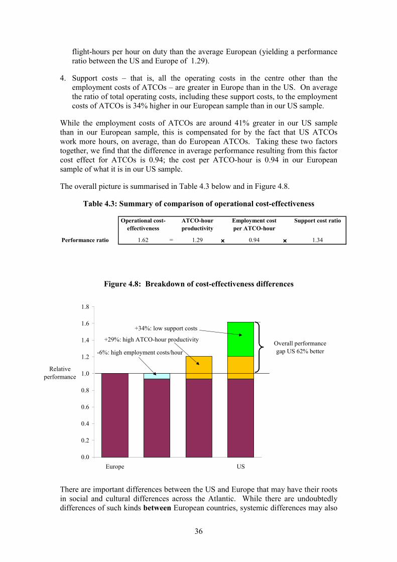
36

flight-hours per hour on duty than the average European (yielding a performanceratio between the US and Europe of 1.29).

4. Support costs � that is, all the operating costs in the centre other than theemployment costs of ATCOs � are greater in Europe than in the US. On averagethe ratio of total operating costs, including these support costs, to the employmentcosts of ATCOs is 34% higher in our European sample than in our US sample.

While the employment costs of ATCOs are around 41% greater in our US samplethan in our European sample, this is compensated for by the fact that US ATCOswork more hours, on average, than do European ATCOs. Taking these two factorstogether, we find that the difference in average performance resulting from this factorcost effect for ATCOs is 0.94; the cost per ATCO-hour is 0.94 in our Europeansample of what it is in our US sample.

The overall picture is summarised in Table 4.3 below and in Figure 4.8.

Table 4.3: Summary of comparison of operational cost-effectiveness

Operational cost-effectiveness



Support cost ratio

Performance ratio 1.62 = 1.29 ×××× 0.94 ×××× 1.34

Figure 4.8: Breakdown of cost-effectiveness differences

0.0

0.2

0.4

0.6

0.8

1.0

1.2

1.4

1.6

1.8

Europe US

Relative performance

-6%: high employment costs/hour

+34%: low support costs

+29%: high ATCO-hour productivity Overall performance gap US 62% better

There are important differences between the US and Europe that may have their rootsin social and cultural differences across the Atlantic. While there are undoubtedlydifferences of such kinds between European countries, systemic differences may also

37

exist. For example, the analysis in the previous section shows that on average UScontrollers work about 32% more hours over the year than European controllers, butcost 41% more. This differing work habit on the two continents may reflect a generaltendency for Europeans to opt for more free time and Americans for more disposableincome and consumption. However, our analysis shows that since the higheremployment costs in the US exceed the higher hours, this difference does notcontribute to explaining the observed performance gap, as measured by operationalcost-effectiveness (62%). This must be sought in explanation of differences inATCO-hour productivity and support costs.

Differences in ATCO-hour productivity can come from two main sources:differences in external conditions (chiefly the complexity and variability of traffic)and differences in technology and working practices. In Chapter 5 we explore thedifferences in traffic complexity and variability. In Chapter 6 we explore in moredetail the 29% differences in ATCO-hour productivity, seeking to break it down intodifferences in what the resources can produce, and differences in how well scarceATCO resources are utilised. In Chapter 7, we look at how working practices are usedto adapt to the variability, and their success in ensuring that resources are best utilised.

In Chapter 8 we examine the information on support costs, to understand how thedifferences in this variable arise. In Chapter 9 we describe the differences in ATFMand their potential impact as a factor contributing to the performance gap in terms ofuse of resources and capacity. In Chapter 10 we outline a number of potential factorswhich have been identified as contributing to explain the performance gap, but whichhave not been fully addressed nor quantified as part of this study. Chapter 11 presentsthe overall conclusions from this study.

38

39

5 Traffic complexity and variability

5.1 Introduction

Differences in the characteristics of the traffic at different centres could have a majorimpact on indicators of cost-effectiveness and productivity. These differences fallinto two major classes:

• differences in what is often termed �complexity� � although there is noconsensus on a definition of this term; and

• differences in the variability of the traffic through a centre � this can have animportant impact on cost-effectiveness, as the more variable the traffic, themore difficult it is to adapt the provision of resources to match the trafficvariability. The difficulty would be even greater if the variability wereunpredictable.

In this chapter we discuss the differences in traffic complexity and variability betweenthe centres selected.

5.2 Traffic complexity

Introduction to complexity

The complexity of the traffic and airspace controlled by a given centre may be a factorthat influences performance.

There is no universally agreed definition of complexity. For the purposes of thisstudy, we have used �complexity� to mean �what makes handling the same number ofaircraft more or less difficult�, with difficulty being defined in terms of controllerworkload.

There are many factors that contribute to complexity, not all of which can easily bemeasured. Not all are completely uncontrollable, although often the measures requiredto mitigate complexity are long-term and require international co-operation, such asairspace redesign. In this study we have focused on a few important factors relating totraffic complexity that can be inferred from readily available data:

• measures of traffic density and the likelihood that the route structure yieldsclose approaches of aircraft (proximity indicators);

• measures of the amount of vertical movement of flights.

These factors have been calculated at centre level.

In this section we discuss first the data used to infer these measures, then themethodology and results for each type of measure at centre level.

We also examined the degree to which individual sectors in our sample arethemselves more or less complex, and in particular whether the sectorisation in the US

40

sample uses systemically different types of sector from that in the European sample.We did this by identifying categories of sector based on quantitative indicators, usingwell-tried statistical techniques. However, there was no indication from this analysisof any systemic difference in the type of sectors employed between Europe and theUS. Details of this analysis, along with further details of the analysis at centre level,are documented in a report by the EUROCONTROL Experimental Centre6.

Data sources for traffic complexity analysis

To perform our analysis we needed data on individual aircraft trajectories (IFRflights) at centre level (excluding TRACON or TMA sectors) for the whole day. Thisinformation could, in principle, be obtained from two sources:

• flight plan data, obtained from the CFMU in Europe

• actual trajectories, obtained from processed radar data.

Radar data was considered to be a more reliable indicator of the traffic complexity.

In the US, radar data at centre level was available for 20017. In Europe, such data8

became available only in 2002, and could not be used for two of the six Europeancentres (Barcelona and Roma). For those centres flight plan data have been used9,and the comparison must be viewed with caution.

To examine the quantitative indicators of traffic complexity, we have used data from arepresentative day where traffic was relatively high10.

For comparability and consistency purposes, the study focused on traffic betweenFL245 and FL470, as some of the centres (Karlsruhe and Maastricht) are upperairspace centres only.

Traffic density indicators

A simple indicator of traffic density is the ratio of km controlled to centre volume(measured in km2×flight levels (100 feet)). However, this simple indicator does notreflect the important consideration that traffic in some centres tended to beconcentrated in parts of the airspace. This concentration is illustrated in Figure 5.1.

6 For more details of the study on traffic complexity, see Traffic Complexity Indicators and Sector TypologyAnalysis, ACE US-Europe Centres Comparisons, T. Chaboud, G. M. Flynn, C. Leleu, L. Zerrouki,EUROCONTROL Experimental Centre Note, to be published in 2003.7 From the Enhanced Traffic Management System (ETMS), operated by the FAA.8 From the Enhanced Tactical Flow Management System (ETFMS) operated by the CFMU.9 To remind the reader of this difference in data, Barcelona and Roma centres are asterisked in the figures wherethe use of flight-plan data is relevant.10 These were for Europe, Wednesday 2 October 2002, and for the USA, Friday 31 August 2001. These were dayson which the traffic was substantially � around 10-20% - greater than the annual average daily value but still fellshort of the peak day of the year.

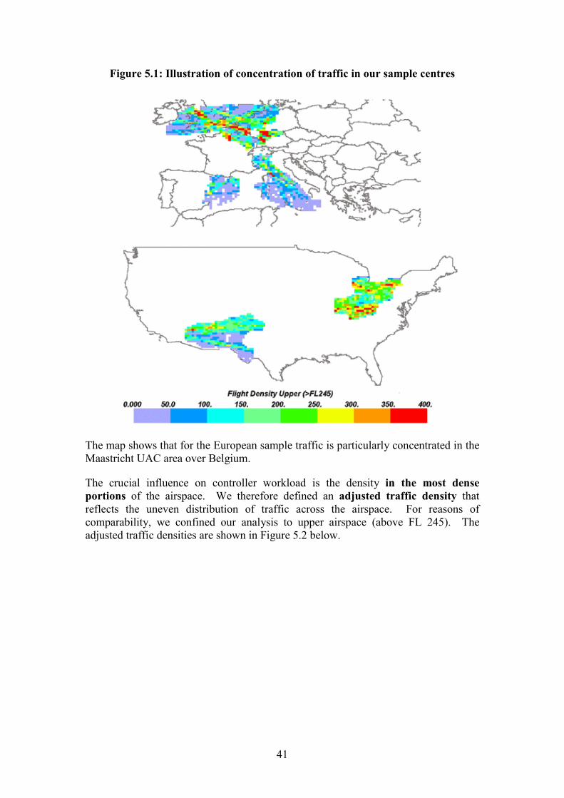
41

Figure 5.1: Illustration of concentration of traffic in our sample centres

The map shows that for the European sample traffic is particularly concentrated in theMaastricht UAC area over Belgium.

The crucial influence on controller workload is the density in the most denseportions of the airspace. We therefore defined an adjusted traffic density thatreflects the uneven distribution of traffic across the airspace. For reasons ofcomparability, we confined our analysis to upper airspace (above FL 245). Theadjusted traffic densities are shown in Figure 5.2 below.

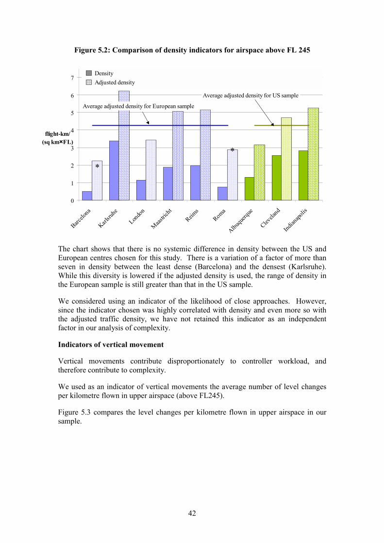
42

Figure 5.2: Comparison of density indicators for airspace above FL 245

0

1

2

3

4

5

6

7

Barcelo

na

Karlsru

he

Londo

n

Maastric

ht

Reims

Roma

Albuqu

erque

Clevela

nd

Indian

apolis

flight-km/(sq km××××FL)

DensityAdjusted density

Average adjusted density for European sample

Average adjusted density for US sample

*

*

The chart shows that there is no systemic difference in density between the US andEuropean centres chosen for this study. There is a variation of a factor of more thanseven in density between the least dense (Barcelona) and the densest (Karlsruhe).While this diversity is lowered if the adjusted density is used, the range of density inthe European sample is still greater than that in the US sample.

We considered using an indicator of the likelihood of close approaches. However,since the indicator chosen was highly correlated with density and even more so withthe adjusted traffic density, we have not retained this indicator as an independentfactor in our analysis of complexity.

Indicators of vertical movement

Vertical movements contribute disproportionately to controller workload, andtherefore contribute to complexity.

We used as an indicator of vertical movements the average number of level changesper kilometre flown in upper airspace (above FL245).

Figure 5.3 compares the level changes per kilometre flown in upper airspace in oursample.

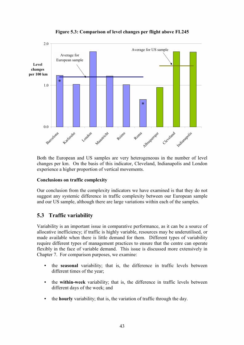
43

Figure 5.3: Comparison of level changes per flight above FL245

0.0

1.0

2.0

Barcelo

na

Karlsru

he

Londo

n

Maastric

htReim

sRom

a

Albuqu

erque

Clevela

nd

Indian

apoli

s

Levelchanges

per 100 km



*

*

Both the European and US samples are very heterogeneous in the number of levelchanges per km. On the basis of this indicator, Cleveland, Indianapolis and Londonexperience a higher proportion of vertical movements.

Conclusions on traffic complexity

Our conclusion from the complexity indicators we have examined is that they do notsuggest any systemic difference in traffic complexity between our European sampleand our US sample, although there are large variations within each of the samples.

5.3 Traffic variability

Variability is an important issue in comparative performance, as it can be a source ofallocative inefficiency; if traffic is highly variable, resources may be underutilised, ormade available when there is little demand for them. Different types of variabilityrequire different types of management practices to ensure that the centre can operateflexibly in the face of variable demand. This issue is discussed more extensively inChapter 7. For comparison purposes, we examine:

• the seasonal variability; that is, the difference in traffic levels betweendifferent times of the year;

• the within-week variability; that is, the difference in traffic levels betweendifferent days of the week; and

• the hourly variability; that is, the variation of traffic through the day.

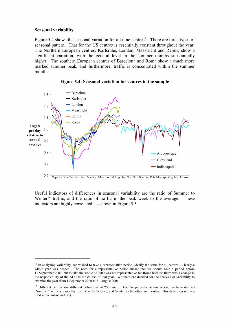
44

Seasonal variability

Figure 5.4 shows the seasonal variation for all nine centres11. There are three types ofseasonal pattern. That for the US centres is essentially constant throughout the year.The Northern European centres: Karlsruhe, London, Maastricht and Reims, show asignificant variation, with the general level in the summer months substantiallyhigher. The southern European centres of Barcelona and Roma show a much moremarked summer peak, and furthermore, traffic is concentrated within the summermonths.

Figure 5.4: Seasonal variation for centres in the sample

0.6

0.7

0.8

0.9

1.0

1.1

1.2

1.3

Flightsper day

relative toannualaverage

Albuquerque

Cleveland

Indianapolis

BarcelonaKarlsruhe

LondonMaastrichtReims

Roma

Sep Oct Nov Dec Jan Feb Mar Apr May Jun Jul Aug Sep Oct Nov Dec Jan Feb Mar Apr May Jun Jul Aug

Useful indicators of differences in seasonal variability are the ratio of Summer toWinter12 traffic, and the ratio of traffic in the peak week to the average. Theseindicators are highly correlated, as shown in Figure 5.5.

11 In analysing variability, we wished to take a representative period, ideally the same for all centres. Clearly awhole year was needed. The need for a representative period meant that we should take a period before11 September 2001, but to take the whole of 2000 was not representative for Roma because there was a change inthe responsibility of the ACC in the course of that year. We therefore decided for the analysis of variability toexamine the year from 1 September 2000 to 31 August 2001.12 Different centres use different definitions of �Summer�. For the purposes of this report, we have defined�Summer� as the six months from May to October, and Winter as the other six months. This definition is oftenused in the airline industry.

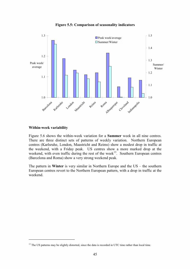
45

Figure 5.5: Comparison of seasonality indicators

1.0

1.1

1.2

1.3

Barcelo

na

Karlsru

he

Londo

n

Maastric

htReim

sRom

a

Albuqu

erque

Clevela

nd

Indian

apoli

s

Peak week/average

1.0

1.1

1.2

1.3

1.4

1.5

Summer/Winter

Peak week/averageSummer/Winter

Within-week variability

Figure 5.6 shows the within-week variation for a Summer week in all nine centres.There are three distinct sets of patterns of weekly variation. Northern Europeancentres (Karlsruhe, London, Maastricht and Reims) show a modest drop in traffic atthe weekend, with a Friday peak. US centres show a more marked drop at theweekend, with even traffic during the rest of the week13. Southern European centres(Barcelona and Roma) show a very strong weekend peak.

The pattern in Winter is very similar in Northern Europe and the US � the southernEuropean centres revert to the Northern European pattern, with a drop in traffic at theweekend.

13 The US patterns may be slightly distorted, since the data is recorded in UTC time rather than local time.

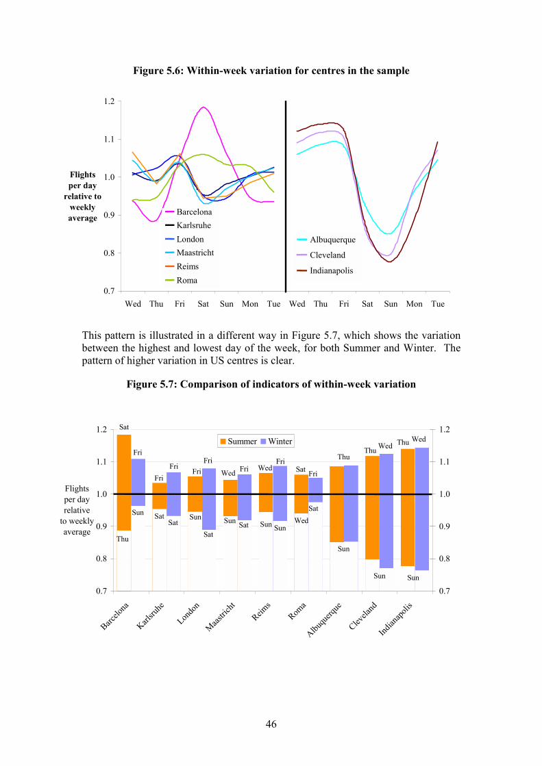
46

Figure 5.6: Within-week variation for centres in the sample

0.7

0.8

0.9

1.0

1.1

1.2

Wed Thu Fri Sat Sun Mon Tue Wed Thu Fri Sat Sun Mon Tue

Flightsper day

relative toweeklyaverage

BarcelonaKarlsruheLondonMaastrichtReimsRoma

Albuquerque

Cleveland

Indianapolis

This pattern is illustrated in a different way in Figure 5.7, which shows the variationbetween the highest and lowest day of the week, for both Summer and Winter. Thepattern of higher variation in US centres is clear.

Figure 5.7: Comparison of indicators of within-week variation

0.7

0.8

0.9

1.0

1.1

1.2

Barcelo

na

Karlsru

he

Londo

n

Maastric

htReim

sRom

a

Albuqu

erque

Clevela

nd

Indian

apoli

s

Flights per dayrelative

to weeklyaverage

0.7

0.8

0.9

1.0

1.1

1.2Summer Winter

Sat

Thu

Fri

Sun

Fri

Sat

Fri

Sun

ThuThu

Sun Sun

WedWed

Thu

Sun

Wed

Sat

Sat

Fri

Sun

WedFri

SunSun

Wed Fri

Sat

Fri

SatSat

Fri

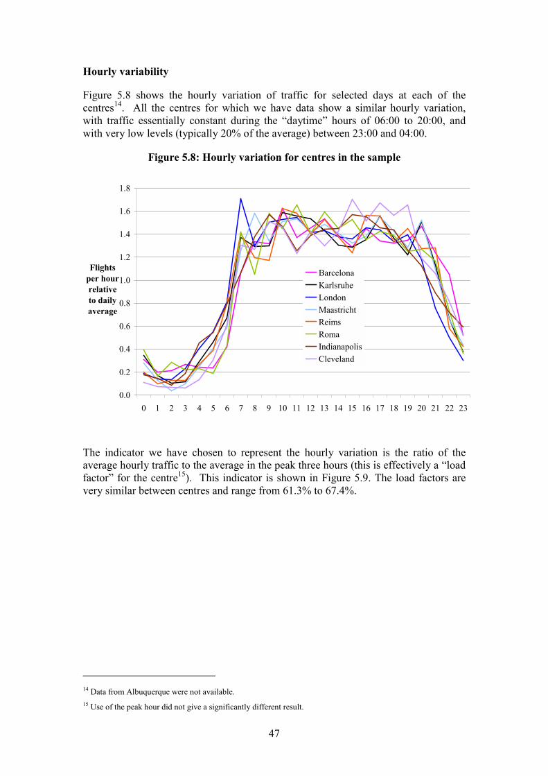
47

Hourly variability

Figure 5.8 shows the hourly variation of traffic for selected days at each of thecentres14. All the centres for which we have data show a similar hourly variation,with traffic essentially constant during the �daytime� hours of 06:00 to 20:00, andwith very low levels (typically 20% of the average) between 23:00 and 04:00.

Figure 5.8: Hourly variation for centres in the sample

0.0

0.2

0.4

0.6

0.8

1.0

1.2

1.4

1.6

1.8

0 1 2 3 4 5 6 7 8 9 10 11 12 13 14 15 16 17 18 19 20 21 22 23

Flightsper hourrelative to dailyaverage

BarcelonaKarlsruheLondonMaastrichtReimsRomaIndianapolisCleveland

The indicator we have chosen to represent the hourly variation is the ratio of theaverage hourly traffic to the average in the peak three hours (this is effectively a �loadfactor� for the centre15). This indicator is shown in Figure 5.9. The load factors arevery similar between centres and range from 61.3% to 67.4%.

14 Data from Albuquerque were not available.15 Use of the peak hour did not give a significantly different result.

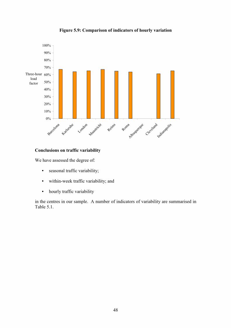
48

Figure 5.9: Comparison of indicators of hourly variation

0%

10%

20%

30%

40%

50%

60%

70%

80%

90%

100%

Barcelo

na

Karlsru

he

Londo

n

Maastric

htReim

sRom

a

Albuqu

erque

Clevela

nd

Indian

apoli

s

Three-hourload

factor

Conclusions on traffic variability

We have assessed the degree of:

• seasonal traffic variability;

• within-week traffic variability; and

• hourly traffic variability

in the centres in our sample. A number of indicators of variability are summarised inTable 5.1.

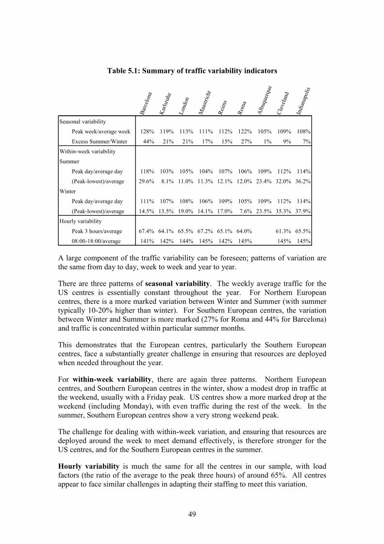
49

Table 5.1: Summary of traffic variability indicators

Barc

elon

a

Kar

lsruh

e

Lond

on

Maa

stric

ht

Reim

s

Rom

a

Alb

uque

rque

Clev

elan

d

Indi

anap

olis

Seasonal variability

Peak week/average week 128% 119% 113% 111% 112% 122% 105% 109% 108%

Excess Summer/Winter 44% 21% 21% 17% 15% 27% 1% 9% 7%

Within-week variability

Summer

Peak day/average day 118% 103% 105% 104% 107% 106% 109% 112% 114%

(Peak-lowest)/average 29.6% 8.1% 11.0% 11.3% 12.1% 12.0% 23.4% 32.0% 36.2%

Winter

Peak day/average day 111% 107% 108% 106% 109% 105% 109% 112% 114%

(Peak-lowest)/average 14.5% 13.5% 19.0% 14.1% 17.0% 7.6% 23.5% 35.3% 37.9%

Hourly variability

Peak 3 hours/average 67.4% 64.1% 65.5% 67.2% 65.1% 64.0% 61.3% 65.5%

08:00-18:00/average 141% 142% 144% 145% 142% 145% 145% 145%

A large component of the traffic variability can be foreseen; patterns of variation arethe same from day to day, week to week and year to year.

There are three patterns of seasonal variability. The weekly average traffic for theUS centres is essentially constant throughout the year. For Northern Europeancentres, there is a more marked variation between Winter and Summer (with summertypically 10-20% higher than winter). For Southern European centres, the variationbetween Winter and Summer is more marked (27% for Roma and 44% for Barcelona)and traffic is concentrated within particular summer months.

This demonstrates that the European centres, particularly the Southern Europeancentres, face a substantially greater challenge in ensuring that resources are deployedwhen needed throughout the year.

For within-week variability, there are again three patterns. Northern Europeancentres, and Southern European centres in the winter, show a modest drop in traffic atthe weekend, usually with a Friday peak. US centres show a more marked drop at theweekend (including Monday), with even traffic during the rest of the week. In thesummer, Southern European centres show a very strong weekend peak.

The challenge for dealing with within-week variation, and ensuring that resources aredeployed around the week to meet demand effectively, is therefore stronger for theUS centres, and for the Southern European centres in the summer.

Hourly variability is much the same for all the centres in our sample, with loadfactors (the ratio of the average to the peak three hours) of around 65%. All centresappear to face similar challenges in adapting their staffing to meet this variation.

50

From data we have access to we have not been able to assess quantitatively the degreeof spatial variability within the centres� airspace, nor the degree of unpredictablevariation, either temporal or spatial.

The extent to which working practices and effective management encourage theprovision of resources (specifically, ATCOs on operational duty) at the times whenthey are needed, in the light of this variability, is discussed in Chapter 7.

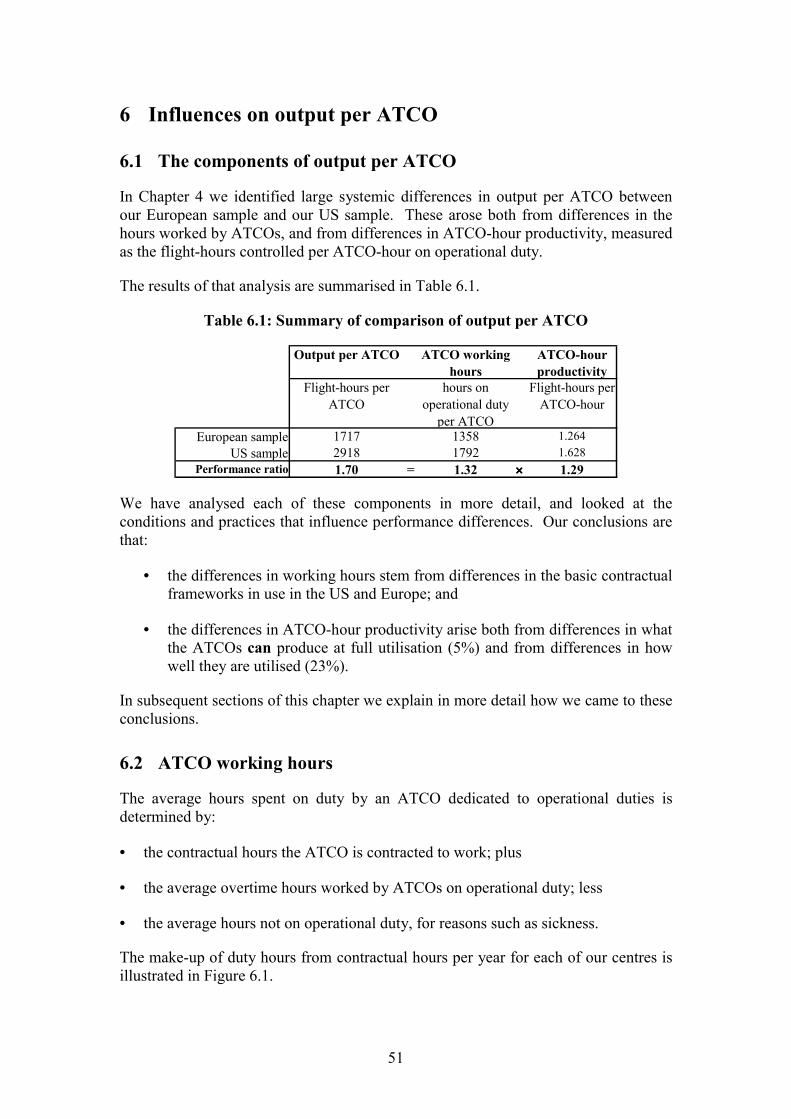
51

6 Influences on output per ATCO

6.1 The components of output per ATCO

In Chapter 4 we identified large systemic differences in output per ATCO betweenour European sample and our US sample. These arose both from differences in thehours worked by ATCOs, and from differences in ATCO-hour productivity, measuredas the flight-hours controlled per ATCO-hour on operational duty.

The results of that analysis are summarised in Table 6.1.

Table 6.1: Summary of comparison of output per ATCO

Output per ATCO ATCO working hours


Flight-hours per ATCO

hours on operational duty

per ATCO

Flight-hours per ATCO-hour

European sample 1717 1358 1.264US sample 2918 1792 1.628


We have analysed each of these components in more detail, and looked at theconditions and practices that influence performance differences. Our conclusions arethat:

• the differences in working hours stem from differences in the basic contractualframeworks in use in the US and Europe; and

• the differences in ATCO-hour productivity arise both from differences in whatthe ATCOs can produce at full utilisation (5%) and from differences in howwell they are utilised (23%).

In subsequent sections of this chapter we explain in more detail how we came to theseconclusions.

6.2 ATCO working hours

The average hours spent on duty by an ATCO dedicated to operational duties isdetermined by:

• the contractual hours the ATCO is contracted to work; plus

• the average overtime hours worked by ATCOs on operational duty; less

• the average hours not on operational duty, for reasons such as sickness.

The make-up of duty hours from contractual hours per year for each of our centres isillustrated in Figure 6.1.

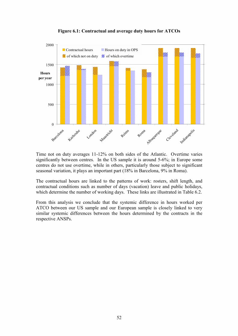
52

Figure 6.1: Contractual and average duty hours for ATCOs

0

500

1000

1500

2000

Barcelo

na

Karlsru

he

Londo

n

Maastric

htReim

sRoma

Albuquer

que

Clevela

nd

Indian

apolis

Hours per year

Contractual hours Hours on duty in OPS

of which not on duty of which overtime

Time not on duty averages 11-12% on both sides of the Atlantic. Overtime variessignificantly between centres. In the US sample it is around 5-6%; in Europe somecentres do not use overtime, while in others, particularly those subject to significantseasonal variation, it plays an important part (18% in Barcelona, 9% in Roma).

The contractual hours are linked to the patterns of work: rosters, shift length, andcontractual conditions such as number of days (vacation) leave and public holidays,which determine the number of working days. These links are illustrated in Table 6.2.

From this analysis we conclude that the systemic difference in hours worked perATCO between our US sample and our European sample is closely linked to verysimilar systemic differences between the hours determined by the contracts in therespective ANSPs.

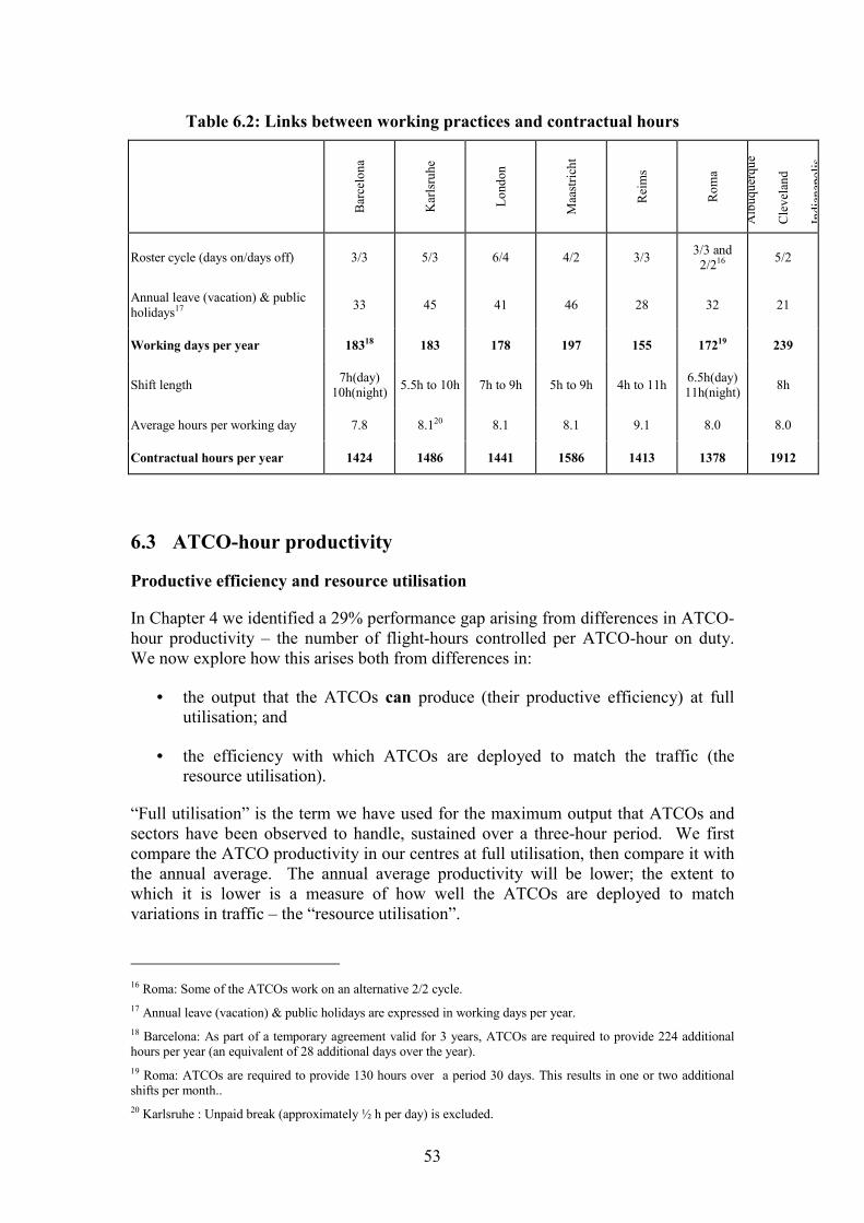
53

Table 6.2: Links between working practices and contractual hours

Bar

celo

na

Kar

lsru

he

Lond

on

Maa

stric

ht

Rei

ms

Rom

a

Alb

uque

rque

Cle

vela

nd

Indi

anap

olis

Roster cycle (days on/days off) 3/3 5/3 6/4 4/2 3/3 3/3 and2/216 5/2

Annual leave (vacation) & publicholidays17 33 45 41 46 28 32 21

Working days per year 18318 183 178 197 155 17219 239

Shift length 7h(day)10h(night) 5.5h to 10h 7h to 9h 5h to 9h 4h to 11h 6.5h(day)

11h(night) 8h

Average hours per working day 7.8 8.120 8.1 8.1 9.1 8.0 8.0

Contractual hours per year 1424 1486 1441 1586 1413 1378 1912

6.3 ATCO-hour productivity

Productive efficiency and resource utilisation

In Chapter 4 we identified a 29% performance gap arising from differences in ATCO-hour productivity � the number of flight-hours controlled per ATCO-hour on duty.We now explore how this arises both from differences in:

• the output that the ATCOs can produce (their productive efficiency) at fullutilisation; and

• the efficiency with which ATCOs are deployed to match the traffic (theresource utilisation).

�Full utilisation� is the term we have used for the maximum output that ATCOs andsectors have been observed to handle, sustained over a three-hour period. We firstcompare the ATCO productivity in our centres at full utilisation, then compare it withthe annual average. The annual average productivity will be lower; the extent towhich it is lower is a measure of how well the ATCOs are deployed to matchvariations in traffic � the �resource utilisation�.

16 Roma: Some of the ATCOs work on an alternative 2/2 cycle.17 Annual leave (vacation) & public holidays are expressed in working days per year.18 Barcelona: As part of a temporary agreement valid for 3 years, ATCOs are required to provide 224 additionalhours per year (an equivalent of 28 additional days over the year).19 Roma: ATCOs are required to provide 130 hours over a period 30 days. This results in one or two additionalshifts per month..20 Karlsruhe : Unpaid break (approximately ½ h per day) is excluded.

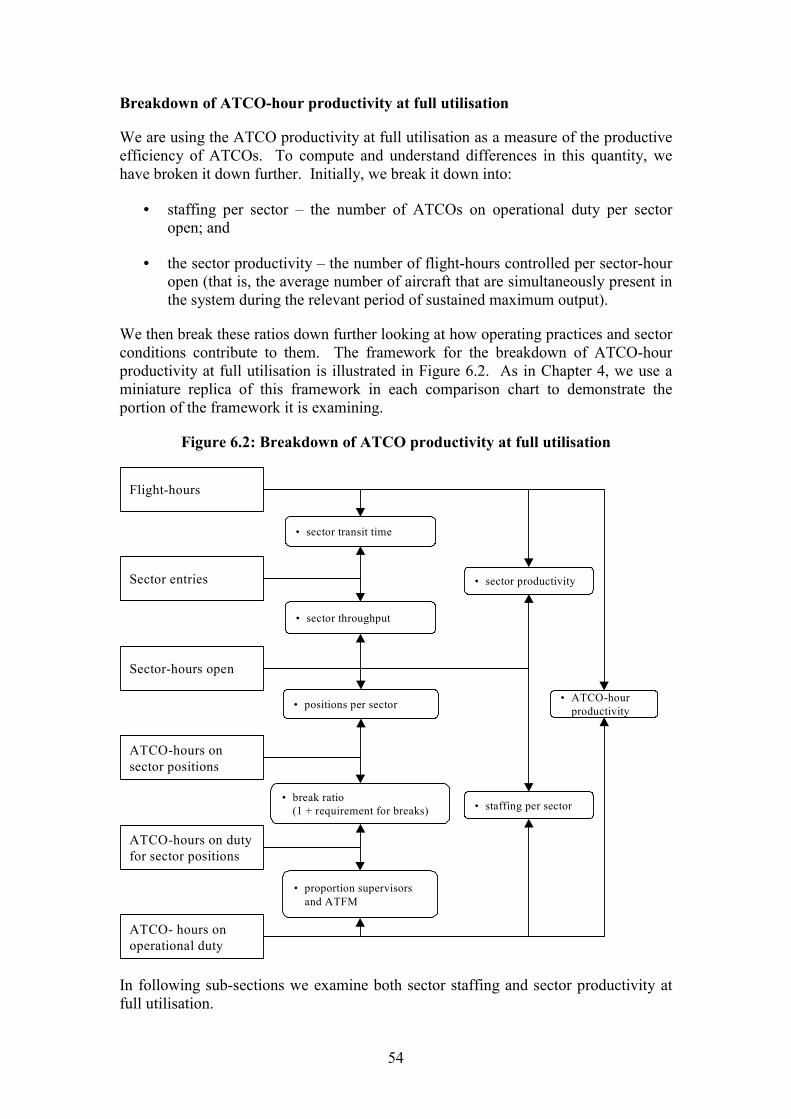
54

Breakdown of ATCO-hour productivity at full utilisation

We are using the ATCO productivity at full utilisation as a measure of the productiveefficiency of ATCOs. To compute and understand differences in this quantity, wehave broken it down further. Initially, we break it down into:

• staffing per sector � the number of ATCOs on operational duty per sectoropen; and

• the sector productivity � the number of flight-hours controlled per sector-houropen (that is, the average number of aircraft that are simultaneously present inthe system during the relevant period of sustained maximum output).

We then break these ratios down further looking at how operating practices and sectorconditions contribute to them. The framework for the breakdown of ATCO-hourproductivity at full utilisation is illustrated in Figure 6.2. As in Chapter 4, we use aminiature replica of this framework in each comparison chart to demonstrate theportion of the framework it is examining.

Figure 6.2: Breakdown of ATCO productivity at full utilisation

Sector-hours open

ATCO-hours onsector positions

ATCO-hours on dutyfor sector positions

ATCO- hours onoperational duty

� proportion supervisorsand ATFM

� positions per sector

� staffing per sector� break ratio

(1 + requirement for breaks)

Flight-hours

Sector entries

� sector throughput

� sector productivity

� sector transit time

� ATCO-hourproductivity

In following sub-sections we examine both sector staffing and sector productivity atfull utilisation.

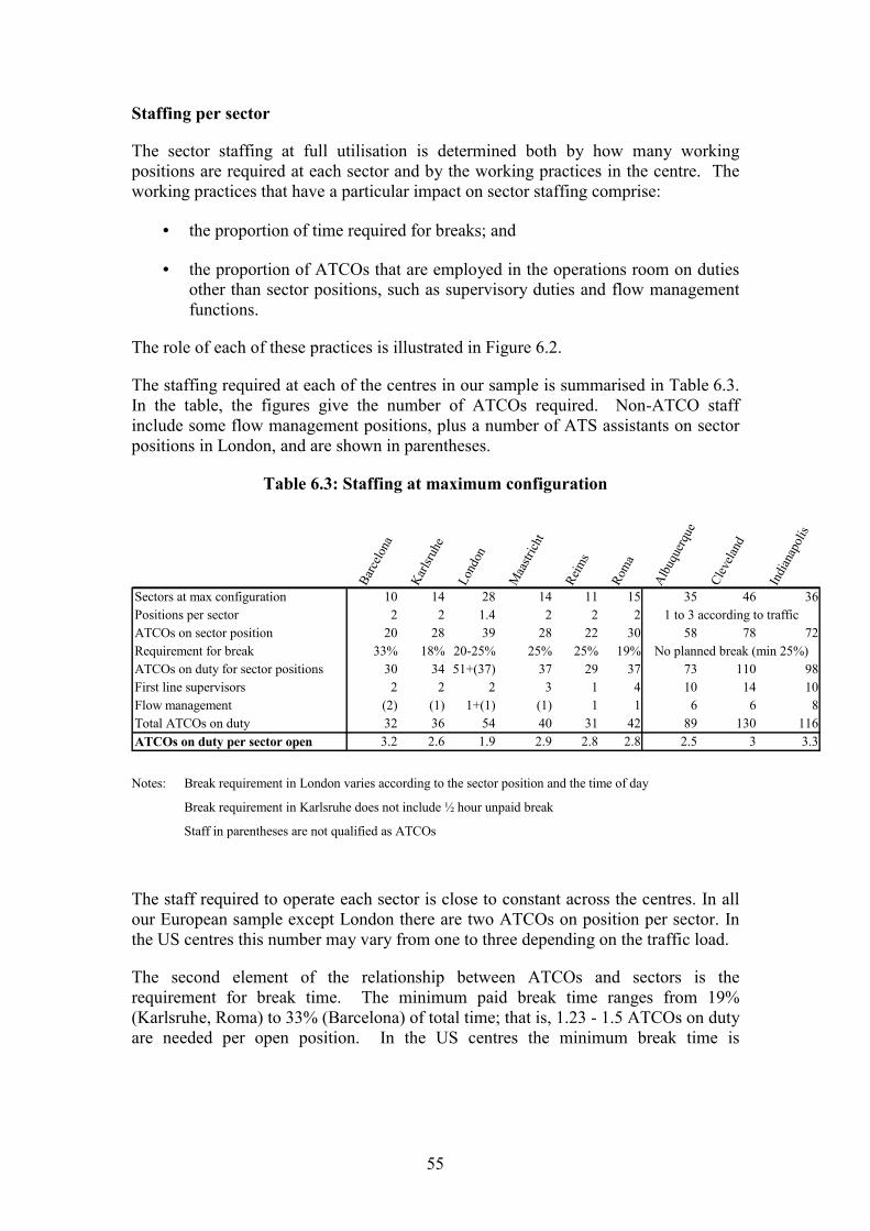
55

Staffing per sector

The sector staffing at full utilisation is determined both by how many workingpositions are required at each sector and by the working practices in the centre. Theworking practices that have a particular impact on sector staffing comprise:

• the proportion of time required for breaks; and

• the proportion of ATCOs that are employed in the operations room on dutiesother than sector positions, such as supervisory duties and flow managementfunctions.

The role of each of these practices is illustrated in Figure 6.2.

The staffing required at each of the centres in our sample is summarised in Table 6.3.In the table, the figures give the number of ATCOs required. Non-ATCO staffinclude some flow management positions, plus a number of ATS assistants on sectorpositions in London, and are shown in parentheses.

Table 6.3: Staffing at maximum configuration

Barc

elona

Karls

ruhe

Lond

on

Maa

strich

t

Reim

s

Rom

a

Albu

quer

que

Clev

eland

Indi

anap

olis

Sectors at max configuration 10 14 28 14 11 15 35 46 36Positions per sector 2 2 1.4 2 2 2ATCOs on sector position 20 28 39 28 22 30 58 78 72Requirement for break 33% 18% 20-25% 25% 25% 19%ATCOs on duty for sector positions 30 34 51+(37) 37 29 37 73 110 98First line supervisors 2 2 2 3 1 4 10 14 10Flow management (2) (1) 1+(1) (1) 1 1 6 6 8Total ATCOs on duty 32 36 54 40 31 42 89 130 116ATCOs on duty per sector open 3.2 2.6 1.9 2.9 2.8 2.8 2.5 3 3.3

No planned break (min 25%)

1 to 3 according to traffic

Notes: Break requirement in London varies according to the sector position and the time of day

Break requirement in Karlsruhe does not include ½ hour unpaid break

Staff in parentheses are not qualified as ATCOs

The staff required to operate each sector is close to constant across the centres. In allour European sample except London there are two ATCOs on position per sector. Inthe US centres this number may vary from one to three depending on the traffic load.

The second element of the relationship between ATCOs and sectors is therequirement for break time. The minimum paid break time ranges from 19%(Karlsruhe, Roma) to 33% (Barcelona) of total time; that is, 1.23 - 1.5 ATCOs on dutyare needed per open position. In the US centres the minimum break time is

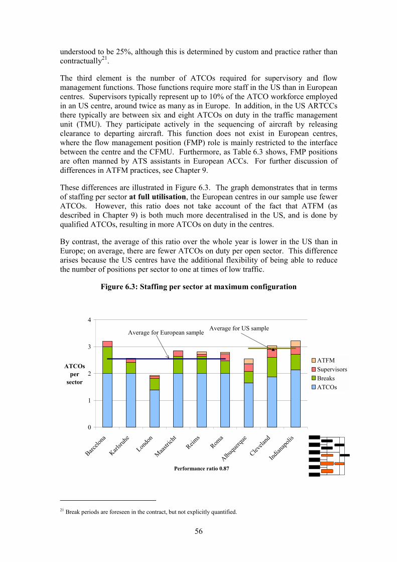
56

understood to be 25%, although this is determined by custom and practice rather thancontractually21.

The third element is the number of ATCOs required for supervisory and flowmanagement functions. Those functions require more staff in the US than in Europeancentres. Supervisors typically represent up to 10% of the ATCO workforce employedin an US centre, around twice as many as in Europe. In addition, in the US ARTCCsthere typically are between six and eight ATCOs on duty in the traffic managementunit (TMU). They participate actively in the sequencing of aircraft by releasingclearance to departing aircraft. This function does not exist in European centres,where the flow management position (FMP) role is mainly restricted to the interfacebetween the centre and the CFMU. Furthermore, as Table 6.3 shows, FMP positionsare often manned by ATS assistants in European ACCs. For further discussion ofdifferences in ATFM practices, see Chapter 9.

These differences are illustrated in Figure 6.3. The graph demonstrates that in termsof staffing per sector at full utilisation, the European centres in our sample use fewerATCOs. However, this ratio does not take account of the fact that ATFM (asdescribed in Chapter 9) is both much more decentralised in the US, and is done byqualified ATCOs, resulting in more ATCOs on duty in the centres.

By contrast, the average of this ratio over the whole year is lower in the US than inEurope; on average, there are fewer ATCOs on duty per open sector. This differencearises because the US centres have the additional flexibility of being able to reducethe number of positions per sector to one at times of low traffic.

Figure 6.3: Staffing per sector at maximum configuration

0

1

2

3

4

Barcelo

na

Karlsru

he

Londo

n

Maastric

htReim

sRom

a

Albuqu

erque

Clevela

nd

Indian

apoli

s


ATCOs per

sector

ATFMSupervisorsBreaksATCOs


21 Break periods are foreseen in the contract, but not explicitly quantified.

57

Sector productivity

We have defined sector productivity as the flight-hours that are handled by the centreper sector-hour open. Viewed another way, this is the number of flights that aresimultaneously being controlled in a given sector, averaged over the sectors of thecentre.

The sector productivity is the product of the sector throughput (the number of sectorentries per hour) and the average transit time for a flight across the sector.

To measure this ratio at full utilisation, we have examined detailed data for a busyweek in summer at each centre. For each sector, we have determined the three-hourperiod in which the throughput (the number of sector entries per hour) was greatest.We have then multiplied this by the average sector transit time for the sector, to obtainthe greatest observed sector productivity. We have then averaged this over the sectorsin the centre, weighting the quantity by the number of flights in the sector. Thiscalculation is summarised in Table 6.4.

Table 6.4: Derivation of sector productivity at full utilisation

Barc

elona

Karls

ruhe

Lond

on

Maa

strich

t

Reim

s

Rom

a

Albu

quer

que

Clev

eland

Indi

anap

olis

Sector throughput (flights/hour) 35 40 34 45 38 40 40 40 48Sector transit time (minutes) 9.6 7.0 7.7 9.2 8.2 10.6 12.6 8.4 8.1Sector productivity at full utilisation (aircraft) 5.5 4.7 4.4 6.9 5.2 7.0 8.3 5.5 6.4

These figures for sector productivity at full utilisation are compared in Figure 6.4, andthe differences in sector throughput and sector transit time that give rise to them inFigure 6.5.

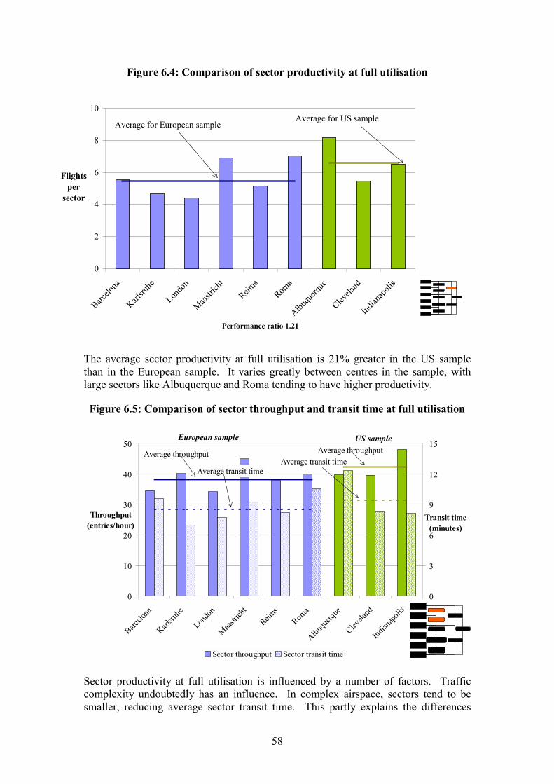
58

Figure 6.4: Comparison of sector productivity at full utilisation

0

2

4

6

8

10

Barcelo

na

Karlsru

he

Londo

n

Maastric

htReim

sRom

a

Albuqu

erque

Clevela

nd

Indian

apoli

s


Flights per

sector


The average sector productivity at full utilisation is 21% greater in the US samplethan in the European sample. It varies greatly between centres in the sample, withlarge sectors like Albuquerque and Roma tending to have higher productivity.

Figure 6.5: Comparison of sector throughput and transit time at full utilisation

0

10

20

30

40

50

Barcelo

na

Karlsru

he

Londo

n

Maastric

ht

Reims

Roma

Albuquer

que

Clevela

nd

Indiana

polis

Throughput (entries/hour)

0

3

6

9

12

15

Transit time (minutes)

Sector throughput Sector transit time

Average throughput Average throughputEuropean sample

Average transit timeAverage transit time

US sample

Sector productivity at full utilisation is influenced by a number of factors. Trafficcomplexity undoubtedly has an influence. In complex airspace, sectors tend to besmaller, reducing average sector transit time. This partly explains the differences

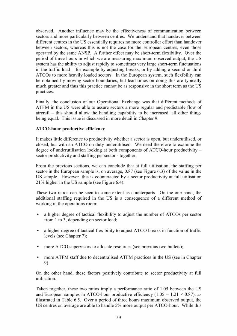
59

observed. Another influence may be the effectiveness of communication betweensectors and more particularly between centres. We understand that handover betweendifferent centres in the US essentially requires no more controller effort than handoverbetween sectors, whereas this is not the case for the European centres, even thoseoperated by the same ANSP. A further effect may be short-term flexibility. Over theperiod of three hours in which we are measuring maximum observed output, the USsystem has the ability to adjust rapidly to sometimes very large short-term fluctuationsin the traffic load � for example by adjusting breaks, or by adding a second or thirdATCOs to more heavily loaded sectors. In the European system, such flexibility canbe obtained by moving sector boundaries, but lead times on doing this are typicallymuch greater and thus this practice cannot be as responsive in the short term as the USpractices.

Finally, the conclusion of our Operational Exchange was that different methods ofATFM in the US were able to assure sectors a more regular and predictable flow ofaircraft � this should allow the handling capability to be increased, all other thingsbeing equal. This issue is discussed in more detail in Chapter 9.

ATCO-hour productive efficiency

It makes little difference to productivity whether a sector is open, but underutilised, orclosed, but with an ATCO on duty underutilised. We need therefore to examine thedegree of underutilisation looking at both components of ATCO-hour productivity �sector productivity and staffing per sector - together.

From the previous sections, we can conclude that at full utilisation, the staffing persector in the European sample is, on average, 0.87 (see Figure 6.3) of the value in theUS sample. However, this is counteracted by a sector productivity at full utilisation21% higher in the US sample (see Figure 6.4).

These two ratios can be seen to some extent as counterparts. On the one hand, theadditional staffing required in the US is a consequence of a different method ofworking in the operations room:

• a higher degree of tactical flexibility to adjust the number of ATCOs per sectorfrom 1 to 3, depending on sector load;

• a higher degree of tactical flexibility to adjust ATCO breaks in function of trafficlevels (see Chapter 7);

• more ATCO supervisors to allocate resources (see previous two bullets);

• more ATFM staff due to decentralised ATFM practices in the US (see in Chapter9).

On the other hand, these factors positively contribute to sector productivity at fullutilisation.

Taken together, these two ratios imply a performance ratio of 1.05 between the USand European samples in ATCO-hour productive efficiency (1.05 = 1.21 × 0.87), asillustrated in Table 6.5. Over a period of three hours maximum observed output, theUS centres on average are able to handle 5% more output per ATCO-hour. While this

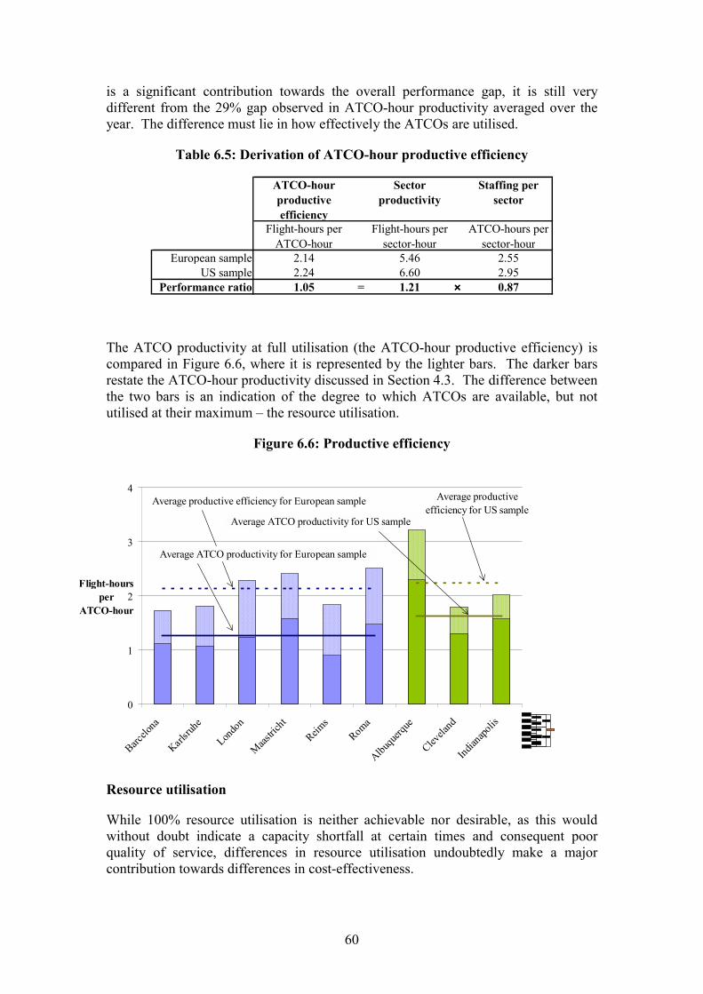
60

is a significant contribution towards the overall performance gap, it is still verydifferent from the 29% gap observed in ATCO-hour productivity averaged over theyear. The difference must lie in how effectively the ATCOs are utilised.

Table 6.5: Derivation of ATCO-hour productive efficiency

ATCO-hour productive efficiency

Sector productivity

Staffing per sector

Flight-hours per ATCO-hour

Flight-hours per sector-hour

ATCO-hours per sector-hour

European sample 2.14 5.46 2.55US sample 2.24 6.60 2.95


The ATCO productivity at full utilisation (the ATCO-hour productive efficiency) iscompared in Figure 6.6, where it is represented by the lighter bars. The darker barsrestate the ATCO-hour productivity discussed in Section 4.3. The difference betweenthe two bars is an indication of the degree to which ATCOs are available, but notutilised at their maximum � the resource utilisation.

Figure 6.6: Productive efficiency

0

1

2

3

4

Barcelo

na

Karlsru

he

Londo

n

Maastric

htReim

sRom

a

Albuquer

que

Clevela

nd

Indianapo

lis

Flight-hours per

ATCO-hour

Average productive efficiency for European sample

Average ATCO productivity for European sample

Average ATCO productivity for US sample

Average productive efficiency for US sample

Resource utilisation

While 100% resource utilisation is neither achievable nor desirable, as this wouldwithout doubt indicate a capacity shortfall at certain times and consequent poorquality of service, differences in resource utilisation undoubtedly make a majorcontribution towards differences in cost-effectiveness.

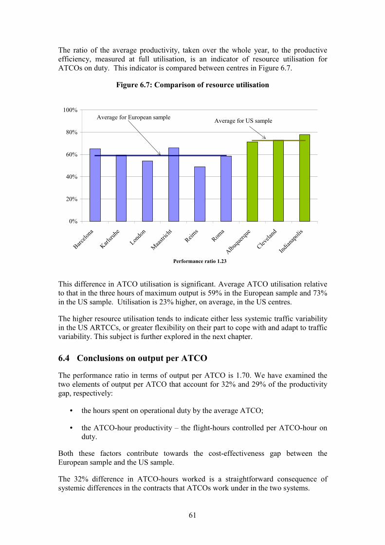
61

The ratio of the average productivity, taken over the whole year, to the productiveefficiency, measured at full utilisation, is an indicator of resource utilisation forATCOs on duty. This indicator is compared between centres in Figure 6.7.

Figure 6.7: Comparison of resource utilisation

0%

20%

40%

60%

80%

100%

Barcelo

na

Karlsru

he

Londo

n

Maastric

htReim

sRom

a

Albuqu

erque

Clevela

nd

Indian

apoli

s


Average for European sample Average for US sample

This difference in ATCO utilisation is significant. Average ATCO utilisation relativeto that in the three hours of maximum output is 59% in the European sample and 73%in the US sample. Utilisation is 23% higher, on average, in the US centres.

The higher resource utilisation tends to indicate either less systemic traffic variabilityin the US ARTCCs, or greater flexibility on their part to cope with and adapt to trafficvariability. This subject is further explored in the next chapter.

6.4 Conclusions on output per ATCO

The performance ratio in terms of output per ATCO is 1.70. We have examined thetwo elements of output per ATCO that account for 32% and 29% of the productivitygap, respectively:

• the hours spent on operational duty by the average ATCO;

• the ATCO-hour productivity � the flight-hours controlled per ATCO-hour onduty.

Both these factors contribute towards the cost-effectiveness gap between theEuropean sample and the US sample.

The 32% difference in ATCO-hours worked is a straightforward consequence ofsystemic differences in the contracts that ATCOs work under in the two systems.

62

The 29% difference in ATCO-hour productivity could be split into two components:the difference in ATCO-hour productive efficiency � what ATCOs were capable ofproducing (5%) � and differences between how well ATCOs were utilised (23%).

We identified the 5% gap in productive efficiency by looking at what the systemswere capable of when the centres were fully utilised (which we assumed happened atthe traffic peaks), in terms of staffing per sector, and sector productivity (flights persector).

• At full utilisation, the staffing per sector is determined by the number ofpositions per sector at full utilisation, the need for breaks, and the number of staffrequired for supervisory and ATFM positions. We found that at full utilisation thestaff required per sector in the European sample was less than that in the USsample, with a performance ratio of 0.87. A major cause of this is that in the USATFM is more devolved to the centres, and is generally staffed by ATCOs.However, we noted too that this difference is reversed taking the average for theyear as a whole; the US centres use fewer ATCOs per sector. This is partly drivenby their ability to reduce the number of positions per sector to one at times of lighttraffic.

• By contrast, the sector productivity at full utilisation in the US sample wassuperior to that in the European sample, with 21% more flights per sector handledat the peak. The net effect of the differences in sector productivity and in staffingper sector made up a 5% gap in ATCO-hour productive efficiency.

The difference between the 5% and the 29% gap in ATCO-hour productivity averagedover the year, discussed in Section 4.3, demonstrates that in Europe, ATCOs are notas fully utilised over the year as the US ATCOs. The ATCO utilisation (the ratio ofthe performance averaged over the year to the performance at full utilisation) is 59%in the European sample and 73% in the US sample (a performance ratio of 1.23).This indicates either that the US system has greater flexibility to adapt to variations intraffic, or that there is less variation to adapt to.

The working practices that permit or inhibit such flexibility, and their possible impacton ATCO utilisation, are discussed in more detail in the next chapter.

63

7 Flexibility in the use of resources

7.1 Introduction

The previous chapter showed that an important part of the performance gap betweenour US sample and our European sample (23%) arose from lower utilisation of theATCOs in Europe. This could arise from two causes:

• there are differences in the traffic conditions that could make it more difficultto adapt levels of staffing to traffic variation;

• European work practices are less flexible in adapting to the variation observed.

To some extent both are true. In Section 5.3 we showed that seasonal variability washigher for European centres, particularly Barcelona and Roma. However, within-week variation was higher in the US centres, and hourly variation much the sameacross the whole sample. All centres require a degree of flexibility in workingpractices to allow them to adapt their staffing to traffic variation. In this chapter weexamine how differences in working practices between the US and Europe havecontributed towards this difference in flexibility, and consequently to the difference inATCO utilisation and hence in overall cost-effectiveness.

7.2 Our findings

In summary, our examination of working practices and their contribution to flexibilityin providing ATCOs in the operations room at the right times to serve the traffic, hasled us to conclude the following:

• working practices in European centres are, in general, not adequate to respondfully to the much greater seasonal variation in Europe (although significantadaptations are made in Barcelona, the centre with the greatest variation);

• working practices in the US allow excellent adaptation to their within-weekvariation, which is in general much greater than in Europe;

• by contrast, many European centres do not adapt staffing levels well towithin-week variation;

• faced with similar hourly variation, some centres have working practices thatare able to adapt better than others, and on average, European centres seem toadapt less well.

In general, we find that European practices are much more heterogeneous than in theUS. Sometimes this heterogeneity is the result of adaptation to different trafficvariability, but not always.

We have observed that the battery of tools available to management in the US centresto deal with variability, particularly unforeseen variation, is wider and moreextensively used than is generally the case in European centres. However, there isundoubtedly scope for improvement on both sides of the Atlantic.

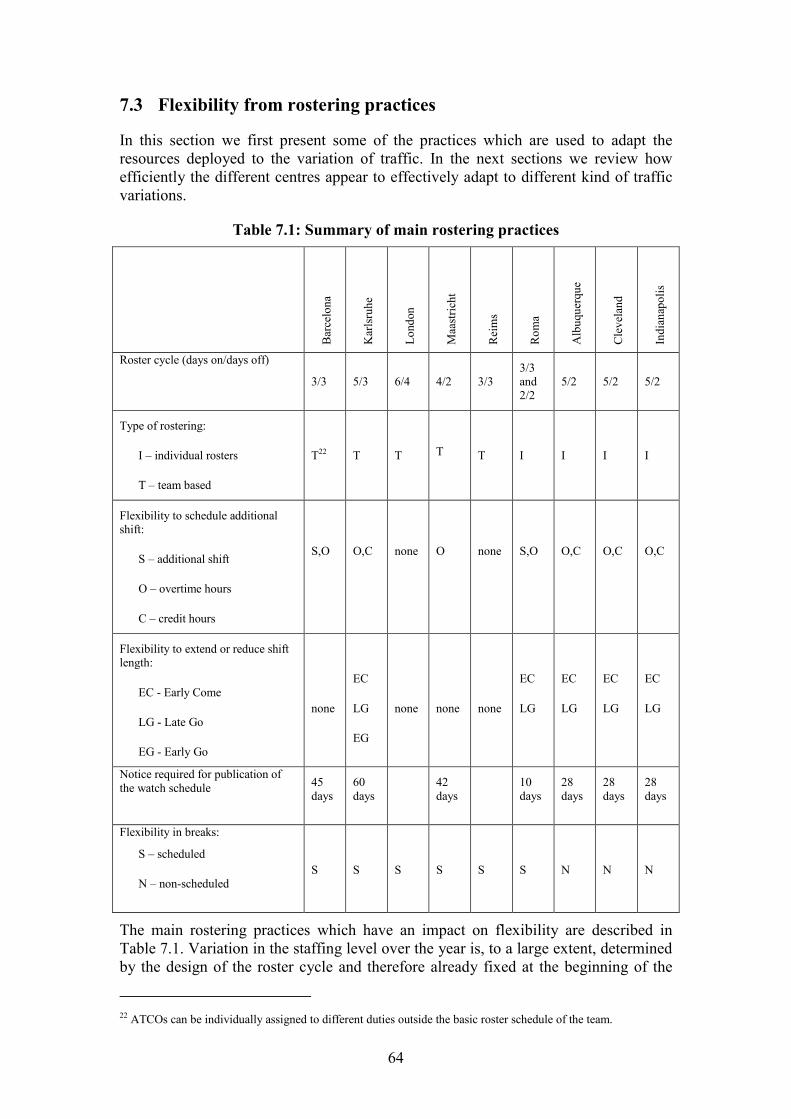
64

7.3 Flexibility from rostering practices

In this section we first present some of the practices which are used to adapt theresources deployed to the variation of traffic. In the next sections we review howefficiently the different centres appear to effectively adapt to different kind of trafficvariations.

Table 7.1: Summary of main rostering practices

Bar

celo

na

Kar

lsru

he

Lond

on

Maa

stric

ht

Rei

ms

Rom

a

Alb

uque

rque

Cle

vela

nd

Indi

anap

olis

Roster cycle (days on/days off)

3/3 5/3 6/4 4/2 3/33/3and2/2

5/2 5/2 5/2

Type of rostering:

I � individual rosters

T � team based

T22 T T T T I I I I

Flexibility to schedule additionalshift:

S � additional shift

O � overtime hours

C � credit hours

S,O O,C none O none S,O O,C O,C O,C

Flexibility to extend or reduce shiftlength:

EC - Early Come

LG - Late Go

EG - Early Go

none

EC

LG

EG

none none none

EC

LG

EC

LG

EC

LG

EC

LG

Notice required for publication ofthe watch schedule 45

days60days

42days

10days

28days

28days

28days

Flexibility in breaks:

S � scheduled

N � non-scheduledS S S S S S N N N

The main rostering practices which have an impact on flexibility are described inTable 7.1. Variation in the staffing level over the year is, to a large extent, determinedby the design of the roster cycle and therefore already fixed at the beginning of the

22 ATCOs can be individually assigned to different duties outside the basic roster schedule of the team.

65

year. In most European centres ATCOs are assigned to a team, and the team they areassigned to will determine which days of the year they have to work. In the US, a listof different roster patterns is established at the beginning of the year, and is assignedto each ATCO as a result of a bidding process based on seniority.

Practices to adapt the basic roster to cope with foreseen variation of traffic and staffunavailability (caused by factors such as sickness and training) vary significantlyacross centres. In most centres (with the exception of Reims and London) additionalshifts may be scheduled through one or more of the following mechanisms:

• Additional shifts: in some centres (Barcelona and Roma), the hours scheduled inthe basic roster comprise only part of the contractual hours. The difference iscovered by additional shifts spread over the year;

• Overtime hours: additional shifts are paid as overtime;

• Credit hours: the additional shifts give the controller �credit hours� that may beused to take an extra day off at a different time.

There is also flexibility in the US and in two European centres to extend the durationof a shift, by requesting an ATCOs either to come earlier (Early Come) or to leavelater (Late Go). Additional hours are either compensated by credit hours or paid asovertime. Reducing the shift length is only possible in Karlsruhe; an ATCO can leaveearlier (Early Go) if operational conditions allow it, and the corresponding number ofhours will be deducted from his or her credit hours.

Finally, the policy on taking breaks, in particular whether they are scheduled, has animpact on the flexibility to adjust resources to match traffic volume. As indicated inTable 7.1, there are two practices: in the European centres, breaks are essentiallyscheduled; in contrast, in the US centres, breaks are unplanned and taken whenconvenient in the light of traffic demand.

7.4 Dealing with seasonal variation

Traffic varies by season, and this variation (as shown in Section 5.3) differs fromcentre to centre.

Working practices that are practically feasible have only a limited ability to deal withhigh seasonal variability. It would be difficult to manage a system where ATCOs arenot required on duty in winter because fewer sectors were required. However, thereare some practices that, to some extent, alleviate the underutilisation, including:

• encouraging or incentivising ATCOs to take holiday (vacation), undergotraining, or undertake other projects during the off-peak season;

• the use of overtime, or rostered time outside the basic contract, in the peakseason.

We find that in our sample, many centres show little success in adapting to seasonalvariation, and in two centres (Maastricht and Cleveland) those measures which aretaken are outweighed by the preference of ATCOs to take holiday in the summer, and

66

there are fewer ATCOs on duty in those two centres in summer than in winter. Roma,which experiences relatively high seasonal variation, adjusts inadequately, butsurprisingly well, given its handicap of being required to permit ATCOs to take leavepreferentially in Summer.

Barcelona, with the most acute seasonal variation, manages to use available methods(restricting leave and training activity, and use of overtime hours) to adapt rather wellto the variation.

In the US centres, poor or no adjustment is not of great consequence since seasonalvariation is low.

7.5 Dealing with within-week variation

As discussed in Chapter 5, there are three distinct patterns of within-week variation inour sample:

• the Northern European pattern of a Friday peak and a low weekend (followedalso by Southern Europe in Winter);

• the South European Summer pattern of a high weekend; and

• the US pattern, which comprises a very low weekend, with even trafficthrough the week.

Within-week variation tends to be higher in the US than in Europe, with the exceptionof Barcelona and Roma during summer weekends. Therefore, all else equal, the needfor adaptability to weekly variation is more pressing in these centres. However,Barcelona and Roma face a particular challenge of their own � that of adapting to twodifferent patterns of within-week variation, one in the summer, one in the winter.

It is evident that a certain set of practices - a single cycle, of length different fromseven days � makes it impossible to adapt systematically to weekly variation intraffic. Such a set of practices is used in a number of European centres (Karlsruhe,London, Maastricht, Reims and Roma). In Barcelona a similar system is used butadditional flexibility is possible as some shifts are not included in the standard roster,but are allocated at the discretion of management to particular days.

To investigate this further, we examined how each of the rostering systems in usewould cope with different types of within-week variation. We found that of thesystems in use in our nine centres, those for four (the US centres and Barcelona) allowessentially perfect adaptation to the kind of within-week variation observed, see forexample Indianapolis in Figure 7.1 below.

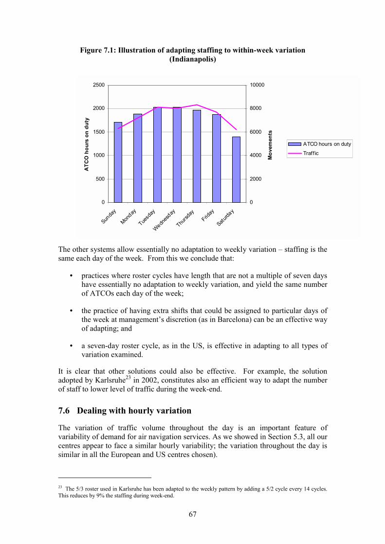
67

Figure 7.1: Illustration of adapting staffing to within-week variation(Indianapolis)

The other systems allow essentially no adaptation to weekly variation � staffing is thesame each day of the week. From this we conclude that:

• practices where roster cycles have length that are not a multiple of seven dayshave essentially no adaptation to weekly variation, and yield the same numberof ATCOs each day of the week;

• the practice of having extra shifts that could be assigned to particular days ofthe week at management�s discretion (as in Barcelona) can be an effective wayof adapting; and

• a seven-day roster cycle, as in the US, is effective in adapting to all types ofvariation examined.

It is clear that other solutions could also be effective. For example, the solutionadopted by Karlsruhe23 in 2002, constitutes also an efficient way to adapt the numberof staff to lower level of traffic during the week-end.

7.6 Dealing with hourly variation

The variation of traffic volume throughout the day is an important feature ofvariability of demand for air navigation services. As we showed in Section 5.3, all ourcentres appear to face a similar hourly variability; the variation throughout the day issimilar in all the European and US centres chosen).

23 The 5/3 roster used in Karlsruhe has been adapted to the weekly pattern by adding a 5/2 cycle every 14 cycles.This reduces by 9% the staffing during week-end.

0

500

1000

1500

2000

2500

Sunda

y

Monday

Tuesd

ay

Wednes

day

Thursd

ayFrid

ay

Saturda

y

ATC

O h

ours

on

duty

0

2000

4000

6000

8000

10000

Mov

emen

ts

ATCO hours on duty

Traff ic

68

The adaptation of resource levels to the variation of demand within the day requiresworking practices that:

• allow for the minimum level of staffing consistent with safe operation duringthe night time;

• allow staff numbers to rise in the morning and fall in the evening at times andrates well adapted to the rise and fall in traffic;

• has patterns of breaks that are consistent with peaks and troughs of trafficduring the day.

The practices that have an impact on this comprise:

• shift lengths and shift starting times (and particularly, flexibility in shiftstarting times); the use of staggered starting times for the shifts provides astraightforward way of adapting to the rapid increase in traffic observed in allcentres in the morning. However, this practice is not universally applied.Furthermore, if the staggering is allowed to be varied at a few weeks� notice(as is done in the US centres), it is an effective way of dealing withforeseeable variations in the pattern between one day and another.

• the policy on taking breaks � in particular whether breaks are scheduled; in theUS centres, flexibility in allocating breaks together with the flexibility to varythe number of ATCOs from one to three per sector according to demand,allows additional flexibility in adapting resources to short-term variation oftraffic;

• the balance of resources allocated to day and night shifts in the rosteringpattern.

Again, a wide variety of practices is found in Europe, while practices in the US areessentially uniform.

We have illustrated the degree to which different centres have adapted their staffingpatterns to the daily variation in traffic in Figure 7.2 (see page 70). These graphsindicate, in each case for a Wednesday in Summer, the way that staffing is adapted totraffic variation24.

Graphs are presented for a selection of centres. Albuquerque and Cleveland areomitted as both the shift patterns and the traffic variation patterns are considered bythe FAA to be sufficiently similar to those for Indianapolis. Features to note include:

• difficulty in matching the �shoulders� in the traffic pattern at the beginningand end of the day (particularly in Barcelona, London, Roma and Reims);

24 The staffing data for these graphs comprise actual data for Indianapolis (17 July 2002), Barcelona (25 July2001), Karlsruhe and Maastricht (5 September 2001), and planned data for Reims (12 June 2002). For Roma, staffon duty are based on actual data and staff on position on planned data (22 August 2001).

69

• occasional large surpluses of controllers caused by overlapping shifts,particularly noticeable in Karlsruhe and Maastricht; and,

• in some centres (all but Karlsruhe), substantial overprovision of controllers atnight; this problem seems to be more acute in Europe.

Factors behind this include:

• long night shifts � the low period of traffic during the night is typically 6-7hours, generally shorter than the shift length. All other things being equal, thelonger the night shift, the worse the utilisation, because staffing is determinedby the highest requirement in the night-shift period;

• rigidity in dealing with the morning rise in traffic, either through inadequate orno use of staggered shift starts, or by misalignment of the shift starts with themorning rise;

• a contractual requirement for longer breaks at night (Barcelona);

• the minimum number of sector positions that have to be kept open at lowperiod of traffic.

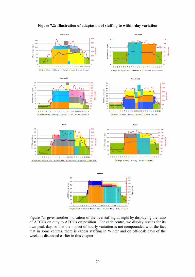
70

Figure 7.2: Illustration of adaptation of staffing to within-day variation

Roma

0

10

20

30

40

50

60

0 1 2 3 4 5 6 7 8 9 10 11 12 13 14 15 16 17 18 19 20 21 22 23 24

ATC

O in

ops

/ in

pos

020406080100120140160

Mov

emen

ts

Night Early 1 Early 2 Late 1 Late 2

Reims

0

5

10

15

20

25

30

35

40

0 1 2 3 4 5 6 7 8 9 10 11 12 13 14 15 16 17 18 19 20 21 22 23 24

ATC

O in

ops

/ in

pos

0

20

40

60

80

100

120

140

160

Mov

emen

ts

Night Shift Early Shift 1 Early Shift 2 Early Shift 3 Day Shift Late Shift

Maastricht

05

101520253035404550

0 1 2 3 4 5 6 7 8 9 10 11 12 13 14 15 16 17 18 19 20 21 22 23 24

ATC

O in

ops

/ in

pos

0

50

100

150

200

250

300

Mov

emen

ts

Night 1 Night 2 Early 1 Early 2 Day 1,2 Late

Karlsruhe

05

101520253035404550

0 1 2 3 4 5 6 7 8 9 10 11 12 13 14 15 16 17 18 19 20 21 22 23 24

ATC

O in

ops

/ in

pos

020406080100120140160180200

Mov

emen

ts

Night Early 1 Early 2 Early 3 Late 1 Late 2 Late 3

Barcelona

0

5

10

15

20

25

30

0 1 2 3 4 5 6 7 8 9 10 11 12 13 14 15 16 17 18 19 20 21 22 23 24

ATC

O in

ops

/ in

pos

0

20

40

60

80

100

120

Mov

emen

ts

Night Early Late Additional 1 Additional 2 Additional 3

Indianapolis

0

20

40

60

80

100

120

140

0 1 2 3 4 5 6 7 8 9 10 11 12 13 14 15 16 17 18 19 20 21 22 23 24

ATC

O in

ops

/ in

pos

0

100

200

300

400

500

600

Mov

emen

ts

Night Early 1 Early 2 Early 3 Late 1 Late 2 Late 3

London

0

10

20

30

40

50

60

70

0 1 2 3 4 5 6 7 8 9 10 11 12 13 14 15 16 17 18 19 20 21 22 23 24

ATC

O in

ops

/ in

pos

050100150200250300350400450

Mov

emen

ts

Night Early 1 Early 2 Early 3 Late 1 Late 2 Day 1 Day 2 Day 3

Figure 7.3 gives another indication of the overstaffing at night by displaying the ratioof ATCOs on duty to ATCOs on position. For each centre, we display results for itsown peak day, so that the impact of hourly variation is not compounded with the factthat in some centres, there is excess staffing in Winter and on off-peak days of theweek, as discussed earlier in this chapter.

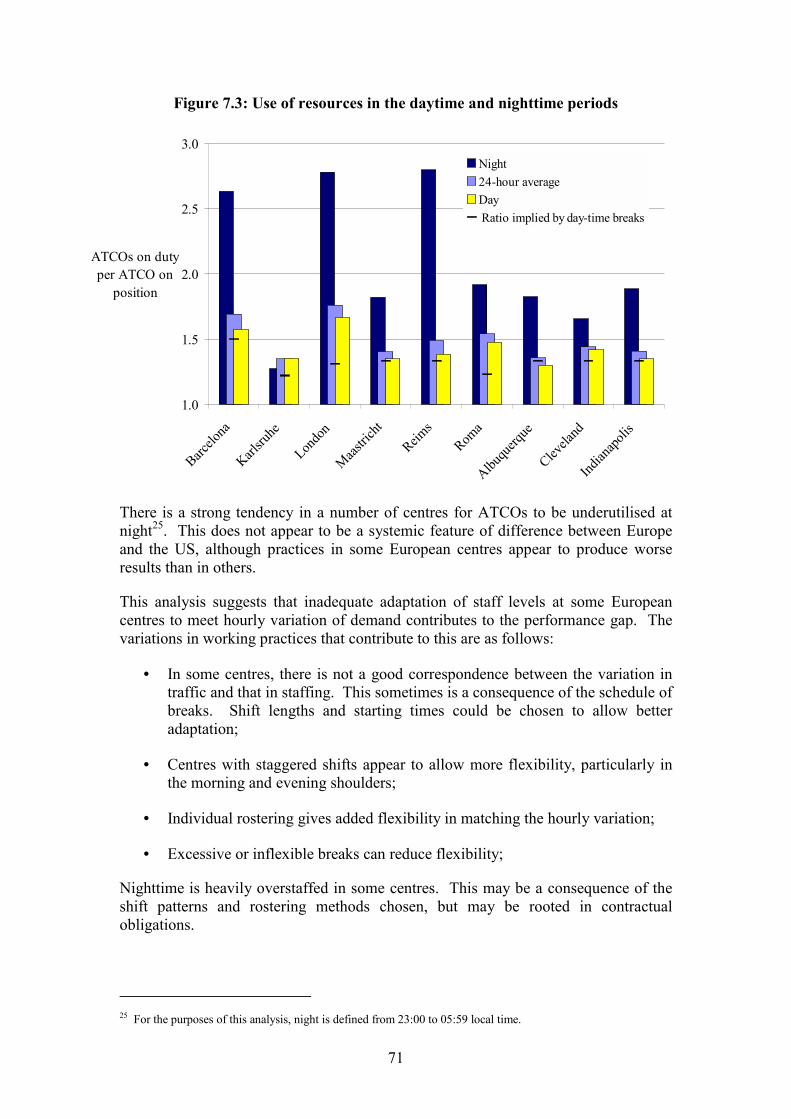
71

Figure 7.3: Use of resources in the daytime and nighttime periods

1.0

1.5

2.0

2.5

3.0

Barcelo

na

Karlsru

he

Londo

n

Maastric

ht

Reims

Roma

Albuqu

erque

Clevela

nd

Indian

apoli

s

ATCOs on dutyper ATCO on

position

Night24-hour averageDay Ratio implied by day-time breaks

There is a strong tendency in a number of centres for ATCOs to be underutilised atnight25. This does not appear to be a systemic feature of difference between Europeand the US, although practices in some European centres appear to produce worseresults than in others.

This analysis suggests that inadequate adaptation of staff levels at some Europeancentres to meet hourly variation of demand contributes to the performance gap. Thevariations in working practices that contribute to this are as follows:

• In some centres, there is not a good correspondence between the variation intraffic and that in staffing. This sometimes is a consequence of the schedule ofbreaks. Shift lengths and starting times could be chosen to allow betteradaptation;

• Centres with staggered shifts appear to allow more flexibility, particularly inthe morning and evening shoulders;

• Individual rostering gives added flexibility in matching the hourly variation;

• Excessive or inflexible breaks can reduce flexibility;

Nighttime is heavily overstaffed in some centres. This may be a consequence of theshift patterns and rostering methods chosen, but may be rooted in contractualobligations.

25 For the purposes of this analysis, night is defined from 23:00 to 05:59 local time.

72

7.7 Conclusions

In the chapter we have examined the ability of working practices to mitigate theadverse impact of traffic variability.

A large component of the traffic demand variability can be foreseen; patterns ofvariation are similar from day to day, week to week, and year to year. It wouldtherefore seem in principle possible to design working methods that could at leastmitigate the impact of variability be allowing the adaptation of staffing patterns to thevariation, although we recognise that practical considerations will prevent perfecttuning of the system even to predictable variation. The optimal practices would varyfrom centre to centre, because the kinds of variation that are faced differ from centreto centre.

Our observation is that practices appear often not to have been designed with thisflexibility in mind, but to have �emerged� from long-established custom and practice.In many centres rosters have remained unchanged for many years and many practicesappear to be less than optimal for current patterns of traffic variation.

Relatively inflexible or poorly adapted practices seem to be more prevalent on theEuropean side, and this may contribute to the performance gap in resource utilisationthat we identified in Chapter 6, and hence to the gaps in productivity and cost-effectiveness.

Flexibility is also important to cope to some degree with unpredictable variation intraffic volume and unpredictable spatial variability. However, there is a clear trade-offbetween costs and quality of service where the unpredictability is significant. Thereare certain practices that permit such flexibility (unplanned breaks, ability to startshifts early and finish them late, and shift starts variable at short notice) that are notuniversally used, particularly in our European sample. This might contribute toobserved differences in productivity, or to quality of service (outside the scope of thisstudy).

Traffic variability is not the same everywhere. Optimal practices will not necessarilybe the same in all the centres. However, all other things being equal, the more tools acentre can deploy, the greater the flexibility, and effective management can increasecost-effectiveness by adopting roster and working practices that make the mosteffective use of the resource, within the constraints of the social framework. In thisrespect, the US seem to have a greater set of tools which they can use to adapt staffingto traffic and other unforeseen circumstances.

73

8 Support cost differences

8.1 Introduction

In Chapter 4 we saw that a major component of the difference in cost-effectiveness atcentre level is differences in �support costs� � that is, the costs that a centre spends onitems other than the employment of ATCOs. We assessed this using the �support costratio� � this is the ratio of all operating costs that we have included in our analysis ofcentres (see Chapter 3 for details) to the employment costs of ATCOs. We found thatin our European sample, the support cost ratio is on average 2.19, as shown inFigure 4.7. For each euro the centres spend on employing ATCOs, they spend anadditional � 1.19 on other things. The support cost ratio for the US sample is 1.64;for each euro spent on ATCOs, an additional � 0.64 is spent on other things. Thisdifference makes a major contribution to the overall difference in operational cost-effectiveness. The �performance ratio� arising from support costs is 1.34 � the lowersupport costs in the US increase its relative cost-effectiveness by 34%, out of a totaldifference of 62%.

In this chapter we analyse more deeply what goes into these support costs, to try togain some understanding of what underlies this performance difference.

8.2 The composition of support costs

In Figure 8.1 we repeat Figure 4.1, the comparison of operational cost-effectiveness,this time breaking down operating costs into ATCO employment costs and supportcosts. This demonstrates the high levels of support costs in the European sampleshown in Figure 4.7 in another way.

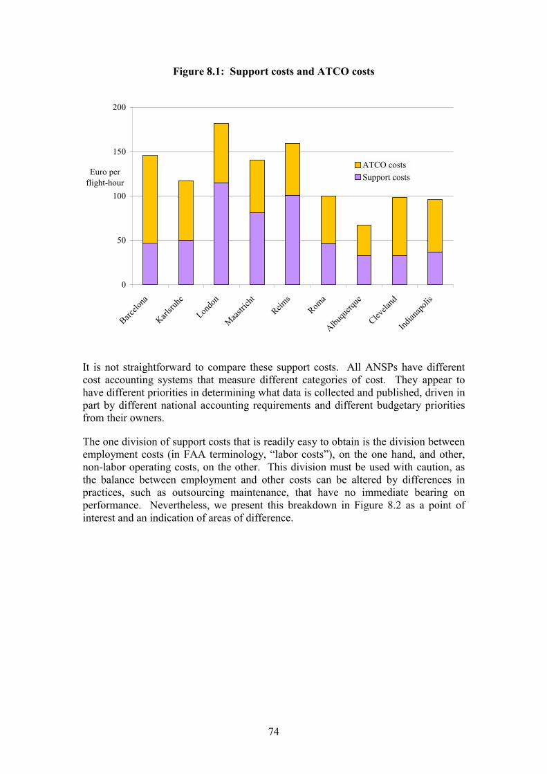
74

Figure 8.1: Support costs and ATCO costs

0

50

100

150

200

Barcelo

na

Karlsru

he

Londo

n

Maastric

htReim

sRom

a

Albuqu

erque

Clevela

nd

Indian

apoli

s


ATCO costsSupport costs

It is not straightforward to compare these support costs. All ANSPs have differentcost accounting systems that measure different categories of cost. They appear tohave different priorities in determining what data is collected and published, driven inpart by different national accounting requirements and different budgetary prioritiesfrom their owners.

The one division of support costs that is readily easy to obtain is the division betweenemployment costs (in FAA terminology, �labor costs�), on the one hand, and other,non-labor operating costs, on the other. This division must be used with caution, asthe balance between employment and other costs can be altered by differences inpractices, such as outsourcing maintenance, that have no immediate bearing onperformance. Nevertheless, we present this breakdown in Figure 8.2 as a point ofinterest and an indication of areas of difference.

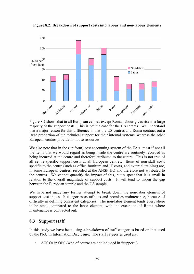
75

Figure 8.2: Breakdown of support costs into labour and non-labour elements

0

20

40

60

80

100

120

Barcelo

na

Karlsru

he

Londo

n

Maastric

htReim

sRom

a

Albuqu

erque

Clevela

nd

Indian

apoli

s


Non-laborLabor

Figure 8.2 shows that in all European centres except Roma, labour gives rise to a largemajority of the support costs. This is not the case for the US centres. We understandthat a major reason for this difference is that the US centres and Roma contract out alarge proportion of the technical support for their internal systems, whereas the otherEuropean centres provide in-house resources.

We also note that in the (uniform) cost accounting system of the FAA, most if not allthe items that we would regard as being inside the centre are routinely recorded asbeing incurred at the centre and therefore attributed to the centre. This is not true ofall centre-specific support costs at all European centres. Items of non-staff costsspecific to the centre (such as office furniture and IT costs, and external training) are,in some European centres, recorded at the ANSP HQ and therefore not attributed tothe centres. We cannot quantify the impact of this, but suspect that it is small inrelation to the overall magnitude of support costs. It will tend to widen the gapbetween the European sample and the US sample.

We have not made any further attempt to break down the non-labor element ofsupport cost into such categories as utilities and premises maintenance, because ofdifficulty in defining consistent categories. The non-labor element tends everywhereto be small compared to the labor element, with the exception of Roma wheremaintenance is contracted out.

8.3 Support staff

In this study we have been using a breakdown of staff categories based on that usedby the PRU in Information Disclosure. The staff categories used are:

• ATCOs in OPS (who of course are not included in �support�)

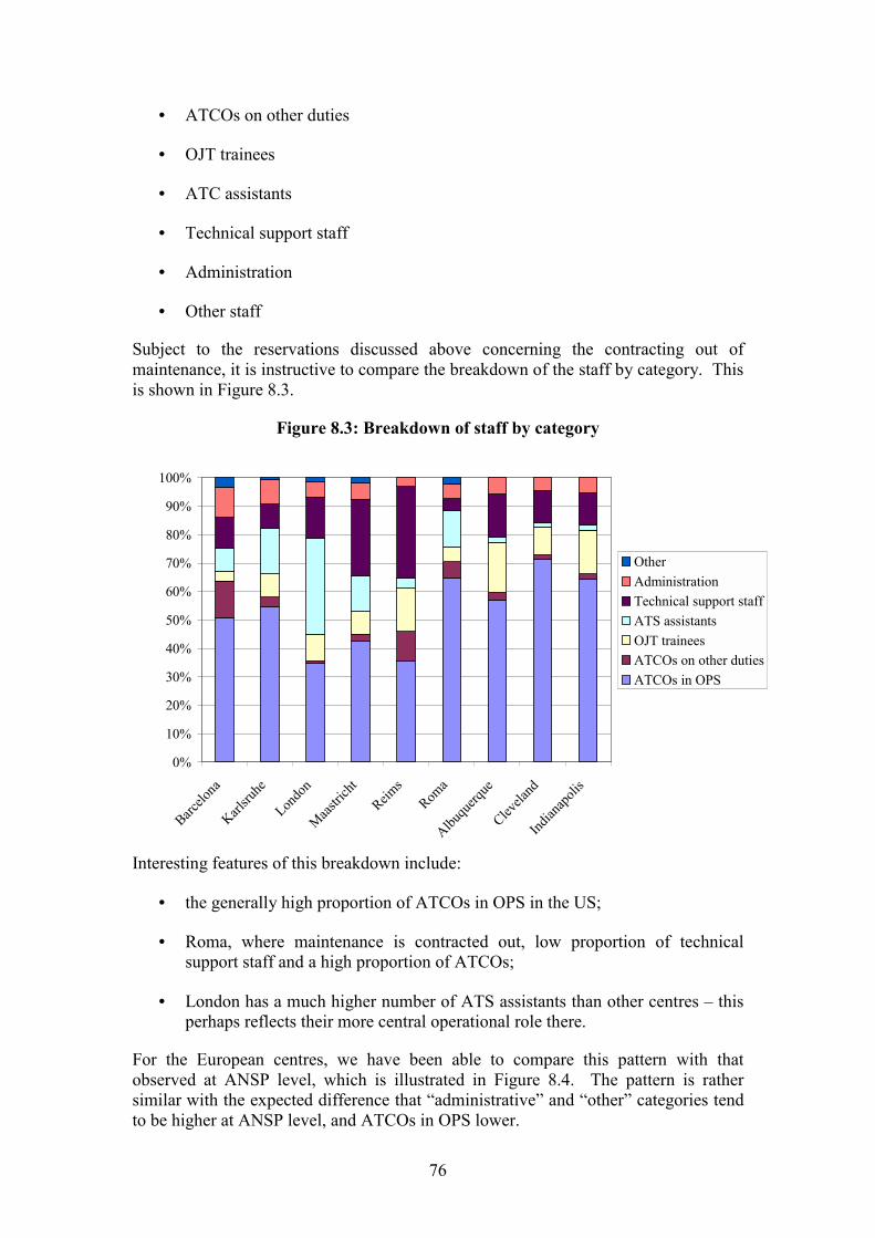
76

• ATCOs on other duties

• OJT trainees

• ATC assistants

• Technical support staff

• Administration

• Other staff

Subject to the reservations discussed above concerning the contracting out ofmaintenance, it is instructive to compare the breakdown of the staff by category. Thisis shown in Figure 8.3.

Figure 8.3: Breakdown of staff by category

0%

10%

20%

30%

40%

50%

60%

70%

80%

90%

100%

Barcelo

na

Karlsru

he

Londo

n

Maastric

htReim

sRom

a

Albuqu

erque

Clevela

nd

Indian

apoli

s

OtherAdministrationTechnical support staffATS assistantsOJT traineesATCOs on other dutiesATCOs in OPS

Interesting features of this breakdown include:

• the generally high proportion of ATCOs in OPS in the US;

• Roma, where maintenance is contracted out, low proportion of technicalsupport staff and a high proportion of ATCOs;

• London has a much higher number of ATS assistants than other centres � thisperhaps reflects their more central operational role there.

For the European centres, we have been able to compare this pattern with thatobserved at ANSP level, which is illustrated in Figure 8.4. The pattern is rathersimilar with the expected difference that �administrative� and �other� categories tendto be higher at ANSP level, and ATCOs in OPS lower.

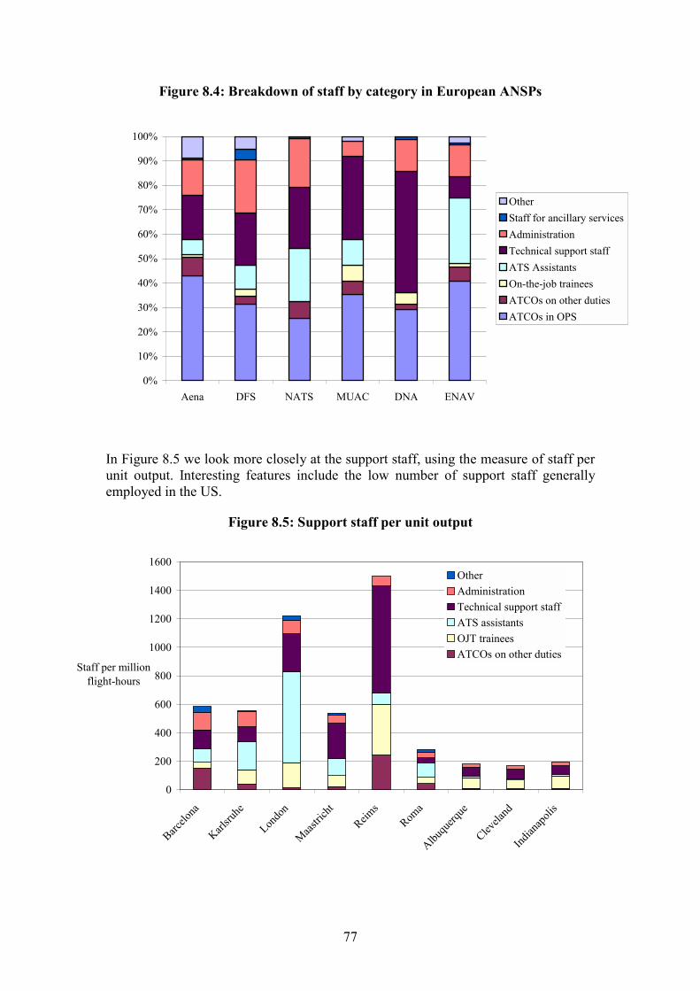
77

Figure 8.4: Breakdown of staff by category in European ANSPs

0%

10%

20%

30%

40%

50%

60%

70%

80%

90%

100%

Aena DFS NATS MUAC DNA ENAV

OtherStaff for ancillary servicesAdministrationTechnical support staffATS AssistantsOn-the-job traineesATCOs on other dutiesATCOs in OPS

In Figure 8.5 we look more closely at the support staff, using the measure of staff perunit output. Interesting features include the low number of support staff generallyemployed in the US.

Figure 8.5: Support staff per unit output

0

200

400

600

800

1000

1200

1400

1600

Barcelo

na

Karlsru

he

Londo

n

Maastric

htReim

sRom

a

Albuqu

erque

Clevela

nd

Indian

apoli

s

Staff per millionflight-hours

OtherAdministrationTechnical support staffATS assistantsOJT traineesATCOs on other duties

78

8.4 Conclusions on support costs

In Chapter 4 we saw that a major component of the difference in cost-effectiveness atthe centre level is the difference in support costs. In our European sample, the centresspend � 1.19 on other things for every � 1 spent on ATCOs, whereas in the US samplethe figure is only � 0.64.

This difference in support costs arises mostly from large numbers of non-ATCO staffin certain European centres. Our analysis has therefore focused on the �labor�element of these support costs, which is generally the largest element. Non-laborcosts tend to be smaller and less consistently defined. We understand that differencesin the recording and attribution of costs will tend to cause these costs to beunderestimated in the European sample compared with the US. Nevertheless, non-labor support costs in the European centres are consistently as high or higher than inthe US centres.

Looking at the difference between the US and the European sample hides a very widevariety of practice in Europe. London and Reims stand out as having both particularlyhigh levels of support staff and of non-labour support costs. The position of Roma,must be viewed in the light of ENAV�s decision to contract out a large proportion oflocal maintenance � this makes the balance between labour and non-labour elementsin the support cost different in Roma from other centres.

This difference, discovered through the work of this study, deserves attention at theservice provider level as well; the differences in support costs may be even largerwhen costs at service provider headquarters are taken into account.

79

9 ATFM differences

9.1 Introduction

ATFM has the same objectives on both sides of the Atlantic: to ensure that trafficflows do not exceed what can be safely handled by controllers, while optimising theuse of available capacity. However, ATFM priorities, as seen by the stakeholders,are not the same. In the US, the priority is to maximize throughput and efficientlyfeed airports to use their capacity fully; in Europe, it is to make sure that traffic doesnot exceed safety-based limitations, mainly on en-route capacity. The effect of ATFMpractices on capacity utilisation is twofold. It may increase global throughput byrerouting aircraft from overloaded to less loaded sectors or by reducing complexityfor a given throughput by sequencing the aircraft on a flow. It may also lead to lesssevere restrictions on traffic if compliance with these restrictions is better, that is, ifthere are fewer overdeliveries, or if dynamic ATFM actions are available to handlesuch overdeliveries. In this chapter we examine the differences between the twosystems which we think may have an impact on productivity.

9.2 Different ATM contexts

For a number of reasons, including operational, geopolitical and climatic factors,ATFM has evolved differently on different sides of the Atlantic. These factorsinclude:

1. In the USA, during summer, thunderstorms routinely impose significant reroutingof entire traffic flows, whereas in Europe, weather conditions do not have such abig impact on en-route flows. AFTM has been optimised to address this problem

2. The US ATM system is geared towards maximizing airport throughput (to makebest use of the scarce resource). Traffic demand is strategically capped at most ofEuropean major airports, which is generally not the case in the USA. The need forATFM actions on flows arriving at major airports is thus less important in Europe,where, by contrast, most capacity constraints occur in en route sectors.

3. There is one data system in the USA, while different systems coexist in Europe. InEurope, the actual traffic picture may be different from the one represented in thedata flow, limiting the opportunity for more dynamic ATFM.

4. Similarly, in many European states, civil ANSPs co-exist with military ANSPs.This tends to make ATC operations more complex and airspace management lesseffective. Moreover, most military airspace in the US is located out of the corearea, which is not the case in Europe, where military airspace affects en routecapacity in dense areas.

5. In Europe, all flight plans are filed according to published routes, whereas in theUS, aircraft operators may choose their routes, outside of ATC preferred routes.However flight plans are still constrained to ATC highly structured preferredroutes in US core areas. In parts of US airspace where operators can freely chosetheir routes, traffic flows are thus more diluted.

80

9.3 The ATFM system in Europe

General description

In Europe, most ATFM is done through ground delay programs. ATFM has beencentrally coordinated by the EUROCONTROL CFMU26 since the mid 90s27. In eachACC, a Flow Management Position (FMP) is in charge of traffic flow managementand interfacing with the CFMU. The FMP is staffed with one or two persons, whichmay not necessarily be qualified controllers (this varies from one ANSP to another) .

ATFM in Europe is carried out in three distinct phases:

• the strategic phase (usually more than seven days ahead);

• the pre-tactical phase (from a few days to a few hours before take-off); and

• the tactical phase (just before take-off and during flight).

Usually no further ATFM measures are decided or implemented after takeoff.

The strategic phase is used to identify potential capacity/demand imbalances and toplan for solutions to alleviate any imbalance.

The pre-tactical phase is the most important one in Europe. Indeed, the mostcommonly used ATFM measure is the imposition of ground delays, for which most ofthe actions are carried out during this pre-tactical phase, as mentioned in the nextparagraph.

The tactical phase is mostly devoted to applying regulations defined in the pre-tacticalphase and to monitoring traffic flow management.

Ground delay programs and ATFM slot allocation process

Ground delay programs, as used in Europe, involve the planning of restrictions ontraffic pre-tactically: in the ACCs, the FMPs check whether their capacities matchdemand for the forthcoming days, based on traffic demand forecasts and staff plannedto be available. The FMPs inform the OPS room supervisor who can then organisesector groups so that capacity is provided where and when it is needed to cope withtraffic demand. If needed, they define restrictions for certain flows, to protect theirairspace, and eventually the airports below it. To some extent, this is done ininteraction with CFMU, which may suggest that a specific ATC sectorisation isdeployed in order to cope with the daily traffic pattern and volume. Though itsimportance is increasing, the role of CFMU in this part of the process is still weak.

The CFMU defines a regulation plan each day, for the whole European system, to beapplied the following day. The regulation plan defines the ground delay programs thatwill be implemented that day. Level capping, tunnelling and re-routings (often

26 Central Flow Management Unit, EUROCONTROL, Brussels.27 Before the creation of the CFMU, ATFM was managed by different states of the European core area at anational level, to protect en-route sectors from traffic overload.

81

advisory, only sometimes compulsory) may also be planned, but are far less oftenused than ground delay.

The regulation plan is submitted to the ACCs, which can request (and obtain) achange in some regulations, and communicated to the aircraft operators, the day priorto its application.

In summer there are teleconferences to address ad-hoc problems (for instance the UK-Balearic Island flow). In such circumstances, aircraft operators are involved from thebeginning in trying to identify solutions. These teleconferences are usually held a fewdays before operations.

Flights affected by a ground delay regulation are given takeoff slots designed to makeflows through the system compliant with the regulations on applicable sectors. Slotsare allocated dynamically by the CFMU a few hours before the flight EOBT28.Ground delays therefore can arise from flow restrictions on en-route bottlenecks, aswell as airports. For each regulation, equity between airspace users is sought, throughslot allocation rules (aircraft are allocated a takeoff slot with a priority linked to theirplanned time at the constrained area). Such rules generally produce a large number ofrelatively low delays rather than greater delays for only a few delayed flights.

The perception among various ATM experts in Europe is that ATFM as currentlyperformed is not completely trusted. There is frequent non-compliance with departureslots; as a result, the number of flights arriving in a sector can exceed the restrictionimposed by a regulation (so-called overdeliveries). As a result, there is a tendency forANSPs to understate the available capacity. This will lead to over-regulation andpoor utilisation of capacity. This is discussed further below in Section 9.5 in theparagraphs on Reactivity and Reliability.

9.4 The ATFM system in the USA

General description

ATFM in the US was initiated to address two main issues: the need to re-route largenumbers of flight around convective weather, and the need to regulate arrival flows atmajor airports.

ATFM is centrally coordinated by the Command Center29. Its goals are:

• to manage traffic flows throughout the entire American airspace;

• to distribute information to all facilities and users; and

• to coordinate ATFM actions.

28 Estimated Off-Block Time.29 Air Traffic Control Systems Command Center, Herndon, VA.

82

Besides ATFM, the Command Center is also responsible for the coordination of otherATM actions, such as airspace sharing with the air force in case of special need(national security or emergency) or route network redesigns.

Each US ARTCC has a Traffic Management Unit (TMU) in its operations room. Atypical TMU is staffed with around six qualified ATCOs, including a TMU manager(Traffic Management supervisor) and an ATCO to keep up to date the status oftemporary restrictions on military airspace. The TMU works in close coordinationwith the Command Center, neighbouring ARTCCs� TMUs and the TWRs of airportslocated below the ARTCC airspace.

Different ATFM actions are taken, depending on the nature of the problem to beaddressed, with priority from the least to the most penalizing measure for the users.This order is:

• Miles in Trail (MIT);

• altitude restrictions (capping, tunnelling);

• re-routing;

• ground stops; and finally

• ground delay programs (GDPs).

Since MIT is the most used ATFM measure, it is described in more detail in the nextsection. GDPs are mostly used in case of severe weather problems and are based onconstraints at a specific destination airport. They are used only when less constrainingATFM measures, such as MIT or level capping, are not possible. GDPs are used as aresponse to severe problems. The usefulness of a Ground Delay Program, as well asthe number of departure airports it covers, may be discussed with users.

A teleconference is held every two hours between the Command Center, users�representatives and all ARTCCs and selected TRACONs. The objective of theseteleconferences is:

• to share a common awareness;

• to analyse the situation (weather or traffic volume issues);

• to discuss and share information on past and active TFM measures; and

• to prepare possible future actions.

The distinction made in Europe between the three ATFM phases (strategic, pre-tactical, tactical phases) is not relevant within US ATFM context.

The US equivalent of the European strategic phase (more than 7 days ahead) sharesthe same goals and principles (see Section 9.3 above). There is no real equivalent ofEuropean pre-tactical phase actions (such as definition of tactical ATFM actions morethan a few hours in advance). Most ATFM actions are prepared tactically, less than afew hours before they are taken.

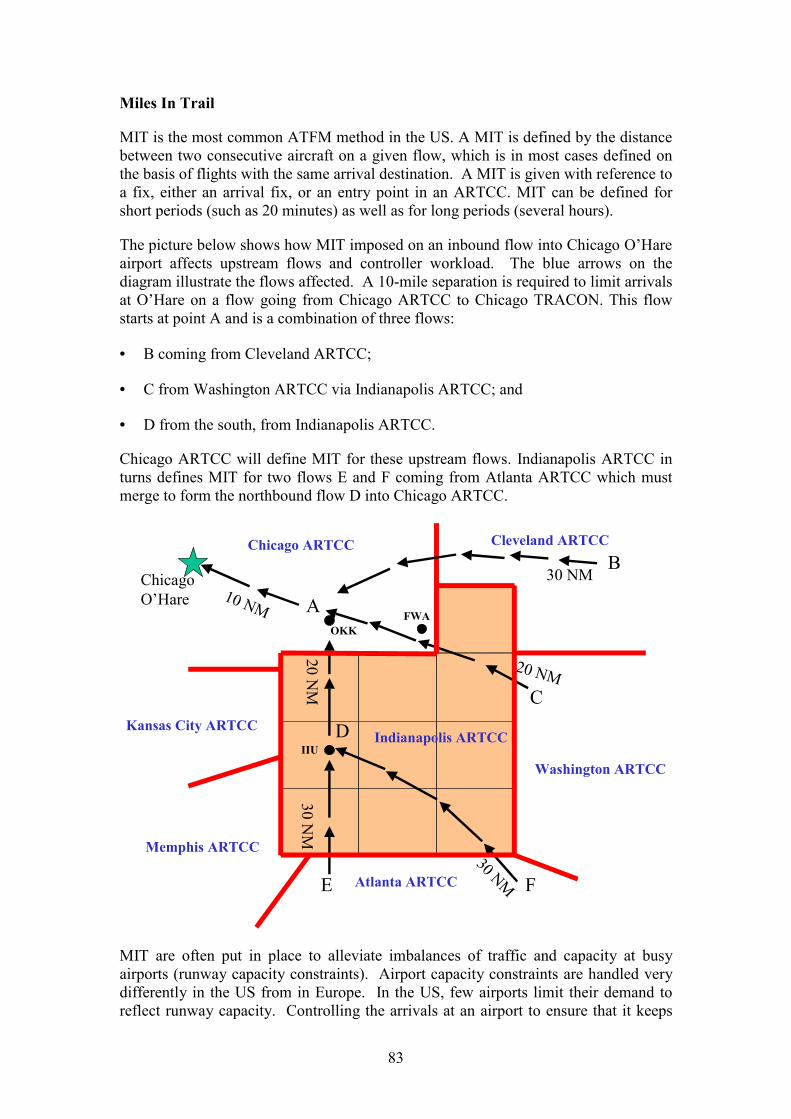
83

Miles In Trail

MIT is the most common ATFM method in the US. A MIT is defined by the distancebetween two consecutive aircraft on a given flow, which is in most cases defined onthe basis of flights with the same arrival destination. A MIT is given with reference toa fix, either an arrival fix, or an entry point in an ARTCC. MIT can be defined forshort periods (such as 20 minutes) as well as for long periods (several hours).

The picture below shows how MIT imposed on an inbound flow into Chicago O�Hareairport affects upstream flows and controller workload. The blue arrows on thediagram illustrate the flows affected. A 10-mile separation is required to limit arrivalsat O�Hare on a flow going from Chicago ARTCC to Chicago TRACON. This flowstarts at point A and is a combination of three flows:

• B coming from Cleveland ARTCC;

• C from Washington ARTCC via Indianapolis ARTCC; and

• D from the south, from Indianapolis ARTCC.

Chicago ARTCC will define MIT for these upstream flows. Indianapolis ARTCC inturns defines MIT for two flows E and F coming from Atlanta ARTCC which mustmerge to form the northbound flow D into Chicago ARTCC.

30 NM

30 NM

20 NM

20 NM

10 NM

ChicagoO�Hare

Chicago ARTCC

Indianapolis ARTCC

Atlanta ARTCC

OKKFWA

IIU

Cleveland ARTCC

30 NM

Washington ARTCC

Memphis ARTCC

A

B

C

D

E F

Kansas City ARTCC

MIT are often put in place to alleviate imbalances of traffic and capacity at busyairports (runway capacity constraints). Airport capacity constraints are handled verydifferently in the US from in Europe. In the US, few airports limit their demand toreflect runway capacity. Controlling the arrivals at an airport to ensure that it keeps

84

within its capacity constraint is seen as a responsibility of air traffic management, notairport management. By contrast, scheduled arrivals at most major European airportsare constrained by a process of slot allocation to be no more than the runway capacity(or other constraint if binding). Thus, traffic demand at the US airport is not�strategically� capped and can significantly exceed capacity at peak time. Theresponsibility for dealing with this is given to the air traffic control system.

MIT are also used to alleviate congestion at a number of en-route bottleneck sectors.This occurs during severe weather (aircraft concentrate in some areas while avoidingthunderstorms), but can also be used in good weather conditions, to cope with hightraffic volumes.

As a MIT is defined for an entire flow, it typically passes back from the TRACON tothe ARTCC above it and to the ARTCCs upstream. This decision largely remainswithin the TMUs.

A MIT can affect aircraft on the ground when an En-route Spacing Program isactivated (ESP). If an aircraft is about to take-off from an airport and to join a flow inthe ARTCC above, on which a MIT restriction is active, the TWR coordinates withthe ARTCC�s TMU before clearing the aircraft to take-off. The ARTCC releases theaircraft when it is possible to enter it into the sequenced flow. If ground delays due toESPs rise dramatically, the local TMU coordinates alternative routings for the mostpenalized flights.

MIT have two contrasting effects on a controller�s workload: on the one hand, MIThelp controllers by providing them better organized flows, but on the other hand MITmay generate extra workload to build the aircraft sequence. Part of this task is done bythe TMUs, through ESP.

The FAA believes that the introduction of MIT has made an important contributiontowards the productivity gains observed in the US system over recent decades.

MIT is perceived by ATCOs as an efficient ATFM measure, because it reducescomplexity and can be finely tuned, thus allowing for a better capacity utilization. It isperceived by the users to be less restrictive than other ATFM measures such asground delays or rerouting because it most often yields lower delays.

9.5 Review of significant differences

Effectiveness of ATFM actions in USA and Europe

In Europe, most ATFM is performed through ground delay programs. Though otherATFM measures, such as rerouting, tunnelling and level capping, are sometimes used,they are not as effectively and as extensively used as in the US.

A fundamental difference between US and Europe is that while MITs are the favouredATFM measure in the US (also from a user perspective), MITs are not applied at allin Europe. It has to be noted that MIT or ESP do not only impact on traffic flowsvolume, as GDP do, but also on traffic complexity, since their direct effect is to avoidbunching.

85

Given the variety of ATFM options, the US Command Center and the ARTCC TMUscan adapt the most effective action to address a specific problem: MIT to avoidbunching of flights over a fix; level capping to keep flow out off selected sectors; re-routing to reduce ground delays due to long MIT queues (through ESP), or to avoid anarea in case of severe weather or of too high traffic volume. ATFM actions such asMIT, rerouting, level capping do not reduce the system throughput: rerouting andcapping allow the use of available capacity in other sectors; MIT reduces complexity.The first goal of ATFM in the US is thus to allow the ATC system to cope with thetraffic that it gets. It is only when the less restrictive measures are not sufficient thatrestrictive ones, such as Ground Delay Programs, are put in place. The latter almostalways result from a severe reduction in capacity at a destination airport.

This diversity of effective ATFM measures not only implies that different actions canbe taken in case of different problems. It also implies that different actions can betaken depending on the moment when they are taken (MIT or even rerouting and levelcapping can be applied to aircraft that are already airborne, when these measures aredecided). This point is developed in the next section.

Reactivity and reliability of dynamic ATFM measures

In Europe, most ATFM actions are decided pre-tactically, based on traffic forecasts.Unavoidably, there will be differences between traffic forecast and actual traffic. As aresult, and given the lack of reactive ways to cope with potential over-deliveries, therewill be restrictions which may not be necessary, leading to an under use of availablecapacity.

In the US, most ATFM procedures (MIT, ESP, level capping, tunnelling and re-routing) are applied dynamically, based on knowledge of actual traffic or on short-term (thus more reliable) traffic forecasts. ATFM measures can be dynamically fine-tuned. Moreover, if a capacity shortfall still occurs, it can be tactically addressed, sothat restrictions can be limited to what is thought to be necessary. In other words, ifthe traffic demand turns out to be higher than expected, specific dynamic ATFMactions are still possible.

The distribution of responsibilities

As they are performed dynamically, most of the ATFM actions in the US are managedand implemented by the centres, under the responsibility of the TMUs. The Americansystem is thus more distributed than the European one, yet it is centrally supervisedand coordinated: ATFM actions decided by a facility have to be coordinated with theCommand Center if they significantly impact another facility or yield a delay higherthan 15 minutes. The ARTCC TMU may have to justify to the Command Center theusefulness of ATFM actions and their importance (duration, number of flows orairport affected). If no agreement arises between different ATC facilities or betweenfacilities and users, regarding the definition and usefulness of ATFM measures, theCommand Center has the power to decide. However, an agreement is almost alwaysreached.

In Europe, CFMU plays a central role in ATFM, through the definition of regulationplans, slot allocation, and some control over the traffic flow limitations asked for bythe ACCs. However, each actor tends to play its part of the process separately: firstthe acceptable hourly flows are decided by the centres, according to their own criteria,

86

and then they are used by CFMU for regulation planning and slot allocation withouteffective involvement of the centres. In case of overdelivery or of under use ofcapacity, there may be no clear division of responsibility among the various actors.

Collaboration and coordination between ATC facilities and airspace users

Close coordination between ATC facilities and airspace users is a key success factorfor effective ATFM. In the US, the Command Center holds on-going teleconferencesfor each of a number of large regions (every two hours and whenever necessary),involving all ATM stakeholders, with the objective of coordinating ATFM actionsbetween ATC facilities and users. Such a coordinated approach lets users discussamongst themselves the possible impact of the proposed ATFM measures. Eachparticipant is responsible for their own actions (for example the centres define theirMIT) as long as it is accepted or agreed by the Command Center, in coordination withother stakeholders.

In Europe, coordination with airspace users takes place, but its scope is more to fine-tune the implementation of the ATFM measures, than to discuss their definition. Theobligation to justify restrictions in front of the users in the frame of periodicteleconferences could help prevent unnecessary ones.

Recently, a trend towards more coordination and collaboration between ATFMstakeholders in Europe has developed. For example, the slot allocation process allowsairlines to choose between re-routings and ground delay when such a trade-off ispossible. Similarly, the CFMU can discuss with the ACCs the allocation of availablestaff to different parts of their airspace and therefore the restrictions on traffic decidedon this basis. Although these practices exist, they are not yet fully and efficientlyused.

9.6 Conclusions

Looking at the American ATFM process, four major differences strike a Europeanobserver:

• ATFM relies more on the tactical phase in the USA, whereas it relies more onthe pre-tactical one in Europe. In the US, the �strategic plans� are decided fourhours before the event. This allows ATFM measures to be based on a moreprecise knowledge of traffic. Moreover, ATFM actions or adjustments to on-going actions can be decided and implemented dynamically. This may have adirect impact on sector productivity, by avoiding unnecessary restrictions ontraffic. The importance of tactical actions is also linked to the fact that thegeneral goal of ATFM in the US is to allow the ATC system to cope with thetraffic that it gets. It is then necessary to offer dynamic ways to treat the flowsso that maximal use of capacity is reached, without constraining the trafficdemand.

• In the US, there is a variety of possible ATFM procedures, which are fine-tuned in response to the problem to be addressed. MIT is the most commonlyused ATFM measure and is designed in a way that non-compliance andunused ATC capacity are minimized, which in turn increases sectorproductivity.

87

• There is an on-going collaborative decision making process, involving allATFM stakeholders. Coordination with users is given a high importance,favouring a trend towards increased efficiency.

• The ATFM is much more decentralized, and at the same time actions arebetter synchronized.

The major enablers of the ATFM process in the US are:

• capacity and staff management at ACC level is designed in a way that themaximum capacity can be more easily utilised when peak traffic occurs (seeSections 5.3 and 6.3);

• the airspace is seamless (consistent airspace classification, same level ofservice and same rules for all controlled traffic30);

• open technical systems, same standards, centralized, but transparent dataflows.

In conclusion, we find that ATFM system in the US tends to work towards betterutilisation of airspace capacity. This in turn has a impact on controller workload.Because peak-time flows are more predictable in the short term, and more regular,controllers in the US are able to handle a larger number of flights simultaneously,contributing to a greater productive efficiency.

30 The notion of military OAT does not exist; when a military aircraft flies in controlled airspace, it must obey civilrules.

88

89

10 Other factors influencing performance

10.1 Introduction

In the previous chapters we analysed the performance gap between our sample ofEuropean centres and our sample of US centres, and identified at which points in theproduction process this performance gap arose. We identified major areas ofdifference in output per ATCO and support costs. The difference in output perATCO arose from longer working hours, greater productive efficiency of the ATCOs,and better utilisation of the ATCOs in the US, although longer working hours werebalanced by high employment costs.

We examined in addition some of the factors, particularly the external factors, such astraffic complexity and variability, and factors related to working practices and ATFM,that could have an influence on these differences.

Inevitably, these factors are numerous and potentially intertwined in a complex way.Moreover, there are subtle differences that are difficult to grasp or to quantify eventhough they can make a large contribution to the observed performance gaps.

In this chapter we examine additional factors that also contribute to the performancegaps identified, and describe their potential influences. We describe first theinfluences identified by the heads of operations during their exchange programme; wethen review the possible influences in the areas of military practices; ATMtechnology, data flow and working methods; and airspace design.

10.2 Influences identified in the operational exchange programme

To further explore factors contributing to the observed performance gap the WorkingGroup set up an exchange programme between head of operations of two Europeancentres - Maastricht UAC and Karlsruhe UAC � and one American centre �Indianapolis ARTCC.

The findings from this exchange programme provided a valuable input into the studyand offered the rationale for much of the analysis of factors influencing performanceboth in previous chapters and in subsequent sections of this chapter.

The findings are documented in a report, available on request from the PRU, whichoutlines the main similarities and differences between these three centres and howthey might influence the observed performance gap. The report�s main conclusionsare:

1. Overall Indianapolis is more flexible and effective in the use of staff resourcesthan the two European centres. Staff planning and management is designed tomatch traffic in the US, while a number of national laws and local collectiveagreements in European centres creates an (unfavourable) environment wherestaff planning and management must adhere to the �rules�. This qualitativeobservation is in line with Chapter 7 results.

90

2. Sector staffing management: in the US sectors are fixed but the number ofcontrollers changes, in Europe the number of controllers is fixed but sectors aredynamically re-configured. This could lead to differences in flexibility (probablybetter adaptation to spatial traffic variation in Europe) and in sector throughput(which is probably higher in US because of the possibility of three ATCOsmanning the sector). This qualitative observation is in line with Chapter 6 andChapter 7 results.

3. ATFM procedures are more effective in the US. This allows the full exploitationof the potential capacity (since, in contrast to Europe, there is no incentive for thecentre to understate capacity) and it allows the full use of available capacity(unnecessary restrictions to traffic are kept to the minimum). This qualitativeobservation is in line with Chapter 9 results.

4. In the US the ATC services provided to military and civil traffic are closelyintegrated and more efficient than in Europe due to a variety of reasons.Furthermore in the US, high military demand is located outside the civil trafficcore area, which is not the case in Europe. These two aspects could partiallyexplain the higher sector throughput in the US.

5. Data interchanges at boundaries between ACCs in Europe tend to involvesubstantial controller workload, sometimes even when the ACCs are operated bythe same organisation. In the US, it is said that the controller workload onhandover between ARTCCs is no greater than that on handover between sectors inthe same ARTCC. This finding could partially explain the higher sectorthroughput and also the higher capacity utilisation observed in the US.

The first three points were discussed in detail in earlier chapters. In this chapter wediscuss the influence of the final two points identified in the operational exchange, aswell as another possible influence: airspace design.

10.3 Military practices

It appears that the success of the US in satisfying civil and military demand relies bothon a more effective organisation of the service and on military demand being outsidethe area of concentrated civil traffic. For instance Albuquerque center providesextensive service to military operations. It includes 175 Special Use Airspace areasand approximately 200 military routes. Clearly, there are also military areas in thetraffic core area of the US (such as the Buckeye military area in Indianapolis ARTCC)where the FAA has to put significant effort into satisfying both types of trafficdemand.

In Europe, for historical reasons, military demand is concentrated in the civil trafficcore area (Karlsruhe, Maastricht and Reims). Satisfying both military and civilairspace requirements has been very challenging during last ten years due to majorincreases in civil traffic, in spite of a simultaneous reduction of military demand dueto the fall of the iron curtain.

Table 10.1 below shows the main differences between American and European ATMcivil-military arrangements. These differences partly explain the increased ATCworkload in dealing with military traffic in Europe. This has an impact on ATCO

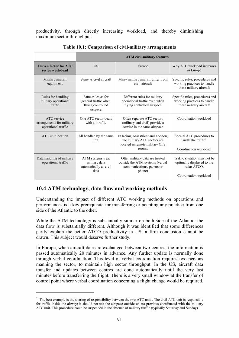
91

productivity, through directly increasing workload, and thereby diminishingmaximum sector throughput.

Table 10.1: Comparison of civil-military arrangements

ATM civil-military features

Driven factor for ATCsector work-load

US Europe Why ATC workload increasesin Europe

Military aircraftequipment

Same as civil aircraft Many military aircraft differ fromcivil aircraft

Specific rules, procedures andworking practices to handle

these military aircraft

Rules for handlingmilitary operational

traffic

Same rules as forgeneral traffic when

flying controlledairspace.

Different rules for militaryoperational traffic even when

flying controlled airspace

Specific rules, procedures andworking practices to handle

these military aircraft

ATC servicearrangements for military

operational traffic

One ATC sector dealswith all traffic

Often separate ATC sectors(military and civil) provide aservice in the same airspace

Coordination workload

ATC unit location All handled by the sameunit.

In Reims, Maastricht and London,the military ATC sectors are

located in remote military OPSrooms.

Special ATC procedures tohandle the traffic31

Coordination workload.

Data handling of militaryoperational traffic

ATM systems treatmilitary data

automatically as civildata

Often military data are treatedoutside the ATM systems (verbal

communications, papers orphone)

Traffic situation may not beoptimally displayed to the

radar ATCO.

Coordination workload

10.4 ATM technology, data flow and working methods

Understanding the impact of different ATC working methods on operations andperformances is a key prerequisite for transferring or adapting any practice from oneside of the Atlantic to the other.

While the ATM technology is substantially similar on both side of the Atlantic, thedata flow is substantially different. Although it was identified that some differencespartly explain the better ATCO productivity in US, a firm conclusion cannot bedrawn. This subject would deserve further study.

In Europe, when aircraft data are exchanged between two centres, the information ispassed automatically 20 minutes in advance. Any further update is normally donethrough verbal coordination. This level of verbal coordination requires two personsmanning the sector, to maintain high sector throughput. In the US, aircraft datatransfer and updates between centres are done automatically until the very lastminutes before transferring the flight. There is a very small window at the transfer ofcontrol point where verbal coordination concerning a flight change would be required.

31 The best example is the sharing of responsibility between the two ATC units. The civil ATC unit is responsiblefor traffic inside the airway; it should not use the airspace outside unless previous coordinated with the militaryATC unit. This procedure could be suspended in the absence of military traffic (typically Saturday and Sunday).

92

This significantly reduces the need for verbal coordination, allowing the US centres tostaff sectors with one ATCO during periods of moderate (and sometimes even heavy)traffic.

The high refreshment rate of information in the US facilitates the conflict detectionand resolution tasks of radar ATCOs, thus reducing ATC workload.

10.5 Airspace design

The design of route structure and ATC sectors makes an important contribution toATCO productivity. The main objectives of airspace design are to minimise controllerworkload by reducing potential conflicts between flights and by reducing the numberof handovers required. Reduced workload will increase the maximum number ofaircraft which can be handled simultaneously by the centre � the sector productivity atfull utilisation, in the terminology of Chapter 6.

The ability of airspace design to improve productivity could be measured in a numberof ways (for example, simulating the traffic complexity with different route structuresand measuring the number of sector movements generated by flights passing througha centre). It was beyond the scope of this study to perform such simulations.

We have not been able to identify any clear difference between methods of airspacedesign in the US and Europe that would give rise to any systemic difference inproductivity. However, we cannot rule out such an effect either.

10.6 Conclusions

In this chapter, we have examined three possible influences on cost-effectiveness thathave not been addressed specifically in the rest of the report:

• military practices;

• ATM technology, data flow, and working methods; and

• airspace design.

We concluded that differences in the first two areas were indeed likely to make acontribution to the observed productivity gap between the US and Europe, althoughwe were not able to quantify the extent of this. We were not able to conclude thatairspace design had any such systemic effect in either direction, but could not rule itout.

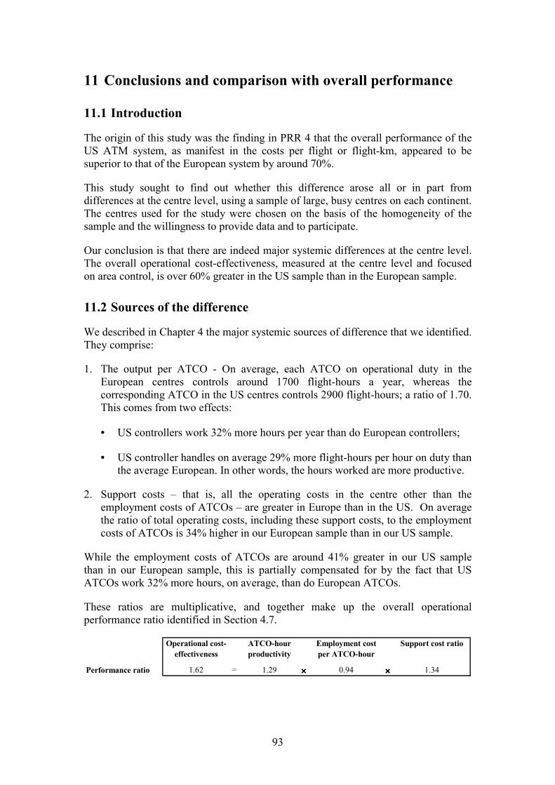
93

11 Conclusions and comparison with overall performance

11.1 Introduction

The origin of this study was the finding in PRR 4 that the overall performance of theUS ATM system, as manifest in the costs per flight or flight-km, appeared to besuperior to that of the European system by around 70%.

This study sought to find out whether this difference arose all or in part fromdifferences at the centre level, using a sample of large, busy centres on each continent.The centres used for the study were chosen on the basis of the homogeneity of thesample and the willingness to provide data and to participate.

Our conclusion is that there are indeed major systemic differences at the centre level.The overall operational cost-effectiveness, measured at the centre level and focusedon area control, is over 60% greater in the US sample than in the European sample.

11.2 Sources of the difference

We described in Chapter 4 the major systemic sources of difference that we identified.They comprise:

1. The output per ATCO - On average, each ATCO on operational duty in theEuropean centres controls around 1700 flight-hours a year, whereas thecorresponding ATCO in the US centres controls 2900 flight-hours; a ratio of 1.70.This comes from two effects:

• US controllers work 32% more hours per year than do European controllers;

• US controller handles on average 29% more flight-hours per hour on duty thanthe average European. In other words, the hours worked are more productive.

2. Support costs � that is, all the operating costs in the centre other than theemployment costs of ATCOs � are greater in Europe than in the US. On averagethe ratio of total operating costs, including these support costs, to the employmentcosts of ATCOs is 34% higher in our European sample than in our US sample.

While the employment costs of ATCOs are around 41% greater in our US samplethan in our European sample, this is partially compensated for by the fact that USATCOs work 32% more hours, on average, than do European ATCOs.

These ratios are multiplicative, and together make up the overall operationalperformance ratio identified in Section 4.7.

Operational cost-effectiveness



Support cost ratio

Performance ratio 1.62 = 1.29 ×××× 0.94 ×××× 1.34

94

11.3 Influences on performance differences

To understand the causes for the performance gap we explored what might underliethese differences.

Social and cultural differences

First, we noted certain social and cultural differences, in particular those whichunderlie the systemically lower hours worked in Europe. These differences reflect, toa large extent, conditions in society and the labour market as a whole, and it would behard to envisage rapid change in these areas.


We developed further the components of ATCO-hour productivity in Chapter 6. Weidentified that the difference arose from the following two factors:

• the productive efficiency of ATCOs in the US centres is around 1.05 timesthose in the European centres

• the remaining difference arises from lower utilisation of the resourcesprovided � in other words, the centres� resources are not deployed aseffectively to match the changing traffic. This effect amounts to a ratio of1.23 in favour of the US centres.

Traffic complexity and variability

We considered traffic complexity as a potential factor influencing performancedifferences. However, the traffic complexity indicators studied do not suggest anysystemic difference in complexity between the European and US centres selected.

We also considered traffic variability. We found that: the seasonal variability wasmore important for the Southern European centres; the within-week variability wasstronger for the US centres; and, the hourly variability was fairly the same across theselected centres.

Flexibility in the use of resources

Adapting the deployment of ATCOs to variations in traffic, and hence achieve thehighest possible resource utilisation, requires working practices that allow forflexibility. Our observation is that practices appear often not to have been designedwith this flexibility in mind, but to have �emerged� from long-established custom andpractice.

Staff planning and management is designed to match traffic in the US, while a numberof national laws and local collective agreements in European centres creates anenvironment where staff planning and management must adhere to the �rules�, ratherthan endeavour to match the traffic.

In many centres rosters have remained unchanged for many years and many practicesappear to be imperfectly adapted to current patterns of traffic variation. In some

95

cases, there were clear indications that adopting better practices from other ANSPs inour sample might bring improvements.

In certain key areas, diversity of practice is most appropriate. Different centres facedifferent conditions (particularly in the area of traffic variability) and require differentpractices to best adapt to their circumstances.

Support costs

It has been beyond the scope of this study to explore support costs in detail, althoughthe differences are striking. A major cause of the difference in support costs appearsto be the numbers of non-ATCO staff in certain European centres. Moreover, non-labor support costs in the European centres are consistently as high or higher than inthe US centres.

There is as much, if not more, diversity among European practices as betweencontinents, although practices and outcomes in the US are rather uniform. A moredetailed insight of the range of activities undertaken in the different centres, includingANSP HQ activities, would be needed to understand more deeply this major source ofdifference in performance.

Other areas

In a number of other areas, we were able to identify practices that were likely tocontribute towards the differences in cost-effectiveness, although the causal link washarder to prove. These included:

• ATFM procedures: improvements in ATFM procedures is perceived as one ofthe major improvement achieved in the US over the last 20 years andcontributed to the increase in US cost-effectiveness. US ATFM proceduresallow both greater sector productivity (because sector workloads were moreeven and predictable) and better capacity utilisation (because unnecessaryrestrictions are avoided).

• civil-military cooperation processes: more integrated and more effective civil-military arrangements in the US.

• interoperability between systems; we were struck by the statement thathandover between centres in the US required no more controller effort thanhandover between sectors. This difference in handover workload would makea difference to the productive efficiency of sectors and hence ATCOs.

11.4 Further areas to explore

We have established that the difference in performance, as measured by operationalcost-effectiveness, between six large, busy centres in Europe and three busy centres inthe US, was around 60% in 2001. This is close to the figure of 70% seen in PRR4 in1999, when looking at the whole of the European and US systems. The PRU hasrecently updated the results of that comparison with 2001 data, and the persistence ofthese ratios is confirmed.

96

This implies that in the elements of performance not measured in this study, and in theareas not covered by our centres, there must also be corresponding or greaterperformance gaps.

There are a number of areas in which we could also look for performance gaps ofequal or greater magnitude. These include:

• other centres: our nine centres account for 6-7% of the en-route cost of thesystems (although the proportion of the traffic they carry is substantiallygreater);

• other elements of en-route operating costs. In this study, we looked at onlythose costs directly incurred at and attributable to the centres. Many costs areincurred at ANSP HQs, in major common facilities like the US CommandCenter or the CFMU, or in maintaining the CNS infrastructure;

• elements of en-route costs other that operating costs � particularly capitalcosts; and

• elements of gate-to-gate air navigation services other than en-route servicesprovided at area control centres � particularly approach control and the costsof terminal navigation services.

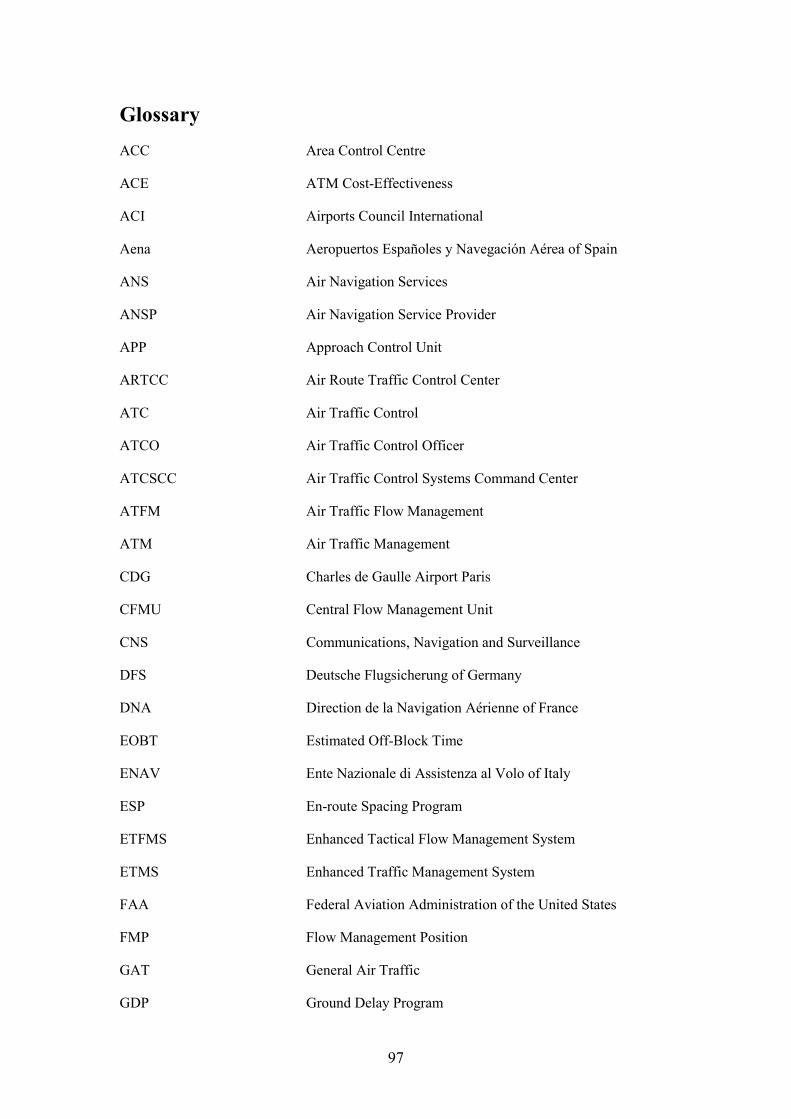
97

GlossaryACC Area Control Centre

ACE ATM Cost-Effectiveness

ACI Airports Council International

Aena Aeropuertos Españoles y Navegación Aérea of Spain

ANS Air Navigation Services

ANSP Air Navigation Service Provider

APP Approach Control Unit

ARTCC Air Route Traffic Control Center

ATC Air Traffic Control

ATCO Air Traffic Control Officer

ATCSCC Air Traffic Control Systems Command Center

ATFM Air Traffic Flow Management

ATM Air Traffic Management

CDG Charles de Gaulle Airport Paris

CFMU Central Flow Management Unit

CNS Communications, Navigation and Surveillance

DFS Deutsche Flugsicherung of Germany

DNA Direction de la Navigation Aérienne of France

EOBT Estimated Off-Block Time

ENAV Ente Nazionale di Assistenza al Volo of Italy

ESP En-route Spacing Program

ETFMS Enhanced Tactical Flow Management System

ETMS Enhanced Traffic Management System

FAA Federal Aviation Administration of the United States

FMP Flow Management Position

GAT General Air Traffic

GDP Ground Delay Program

98

HQ Headquarters

IFR Instrument Flight Rules

km Kilometre

LATCC London Area and Terminal Control Centre

LVNL Luchtverkeersleiding Nederland

MIT Miles in Trail

MOA Military Operating Area

MUAC Maastricht Upper Area Control Centre

NATS National Air Traffic Services Limited of the UK

nm Nautical Miles

OAT Operational Air Traffic

OJT On-the-job trainee or On-the-job training

OPS Operations

PRC Performance Review Commission

PRR Performance Review Report

PRU Performance Review Unit

R&D Research and Development

SUA Special Use Airspace

TFM Traffic Flow Management

TMA Terminal Manoeuvring Area

TMU Traffic Management Unit

TRACON Terminal Radar Approach Control

TWR Traffic Controlled Tower

UAC Upper Area Control Centre

US United States of America

99

ANNEX A: Factsheets for the centres selected

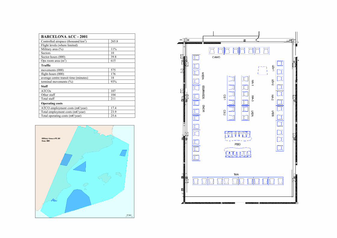
BARCELONA ACC - 2001Controlled airspace (thousand km2) 265.8Flight levels (where limited)Military area (%) 11%Sectors 10Sector-hours (000) 39.8Ops room area (m2) 615Trafficmovements (000) 575flight-hours (000) 176average centre transit time (minutes) 18terminal movements (%) 93%StaffATCOs 107Other staff 104Total staff 211Operating costsATCO employment costs (m�/year) 17.4Total employment costs (m�/year) 23.9Total operating costs (m�/year) 25.6

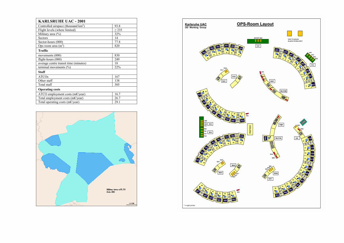
KARLSRUHE UAC - 2001Controlled airspace (thousand km2) 93.8Flight levels (where limited) ≥ 235Military area (%) 32%Sectors 14Sector-hours (000) 77.8Ops room area (m2) 820Trafficmovements (000) 830flight-hours (000) 249average centre transit time (minutes) 18terminal movements (%) 22%StaffATCOs 167Other staff 138Total staff 305Operating costsATCO employment costs (m�/year) 16.7Total employment costs (m�/year) 26.7Total operating costs (m�/year) 29.1

OPS-Room LayoutKarlsruhe UACOD Working Group

* = night printer

FR1

RM

7900

FC3

27

FE3

26

FE2

25

24

FC2

23

FE1

22

FC1

20

FC0

21

FE0

WLFDB

RKP

ER1

GR1

DR1

CCS1

EK1

DK1

CR1

16

1011

12

13

14

15

17

09

ZC001

ZE0

02

ZE1

03

ZC1

04

ZE2

05

ZC2

ZA1 ZB1ZA2

EA4

RC1

RE1

UE2

UC2

UC1

UE1ZC3

ZE3UA1

RA1UA2

EA3

RA2

EA1FK1

FA2*FA1*

EA2UK1

MA4

FB3

TA1

TB1

TA2

WA1

WA2

SK1

SA2*SA1*

SK2

SB1*TA2*

TA1*

SC3

6564

SE3

63

SE2

62

SC2

60

SC161

SE1

SR1

NB1NA2

NA1

NA1

WA4NK2

NC333

NE334

NE2

55

54

NC253

NE152

NC150

NC0

51

NE0

CE330

CC331

CE432

DA

MA3FA1

FA3FA2

CB2

CCS2

TC346

TE3

47

TE2

42

43

TC2

44

TE1

45

TC1

40

TE0

41

TC0

FMP

WLFVK

DR3

SVS

WK

1

SVS

WR1

WS1

Info-TerminalsDAISY/INTRANET

CB1

DK2

DR2

41

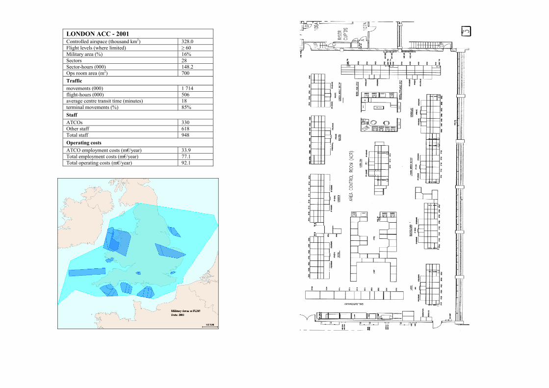
LONDON ACC - 2001Controlled airspace (thousand km2) 328.0Flight levels (where limited) ≥ 60Military area (%) 16%Sectors 28Sector-hours (000) 148.2Ops room area (m2) 700Trafficmovements (000) 1 714flight-hours (000) 506average centre transit time (minutes) 18terminal movements (%) 85%StaffATCOs 330Other staff 618Total staff 948Operating costsATCO employment costs (m�/year) 33.9Total employment costs (m�/year) 77.1Total operating costs (m�/year) 92.1

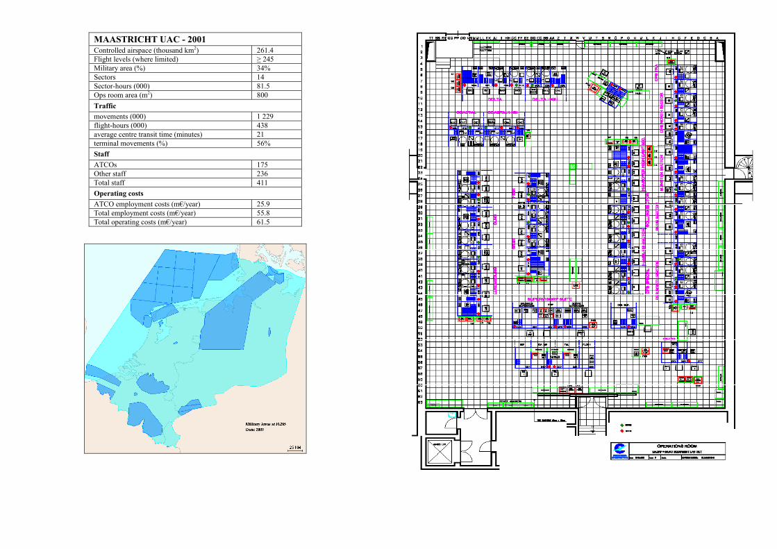
MAASTRICHT UAC - 2001Controlled airspace (thousand km2) 261.4Flight levels (where limited) ≥ 245Military area (%) 34%Sectors 14Sector-hours (000) 81.5Ops room area (m2) 800Trafficmovements (000) 1 229flight-hours (000) 438average centre transit time (minutes) 21terminal movements (%) 56%StaffATCOs 175Other staff 236Total staff 411Operating costsATCO employment costs (m�/year) 25.9Total employment costs (m�/year) 55.8Total operating costs (m�/year) 61.5

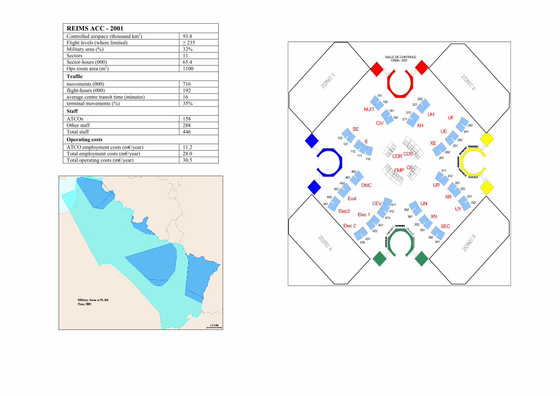
REIMS ACC - 2001Controlled airspace (thousand km2) 93.8Flight levels (where limited) ≥ 235Military area (%) 32%Sectors 11Sector-hours (000) 65.4Ops room area (m2) 1100Trafficmovements (000) 716flight-hours (000) 192average centre transit time (minutes) 16terminal movements (%) 35%StaffATCOs 158Other staff 288Total staff 446Operating costsATCO employment costs (m�/year) 11.2Total employment costs (m�/year) 28.0Total operating costs (m�/year) 30.5

SALLE DE CONTROLE

CRNA - EST

XN

UN

UR

UY

Eval

Elec3

DMC

UH

UE

XEE

CiV

NUIT

SEXH

XR

Elec 2

UF

CEV

Elec 1

311

332

331

322

321

312

362

341342

351

352

361

452

451

441

442

421

422

432431

462

461

411

412

413

110

112111

121

122

151

152

162

161

211

212

221

222

261

262

251

252

241

242

CDS

FMP CE

CDR

SEC

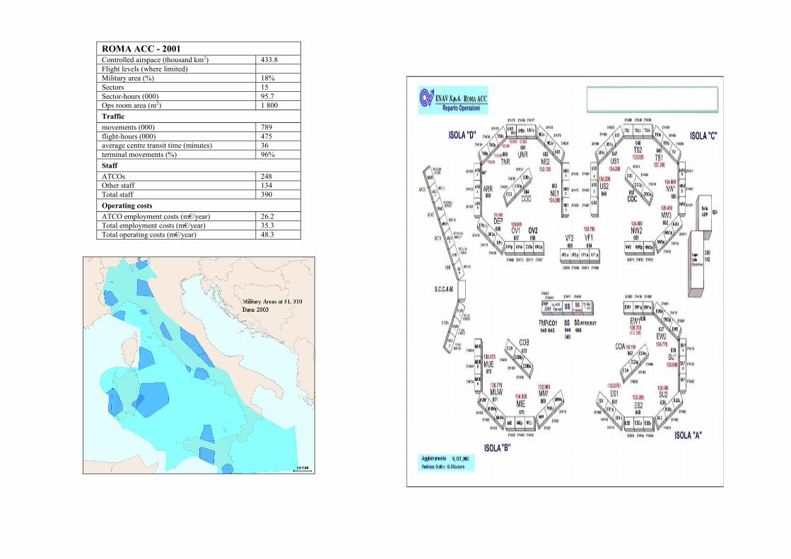
ROMA ACC - 2001Controlled airspace (thousand km2) 433.8Flight levels (where limited)Military area (%) 18%Sectors 15Sector-hours (000) 95.7Ops room area (m2) 1 800Trafficmovements (000) 789flight-hours (000) 475average centre transit time (minutes) 36terminal movements (%) 96%StaffATCOs 248Other staff 134Total staff 390Operating costsATCO employment costs (m�/year) 26.2Total employment costs (m�/year) 35.3Total operating costs (m�/year) 48.3

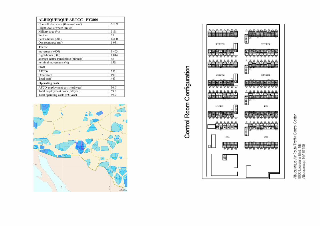
ALBUQUERQUE ARTCC - FY2001Controlled airspace (thousand km2) 618.9Flight levels (where limited)Military area (%) 51%Sectors 35Sector-hours (000) 161.0Ops room area (m2) 1 031Trafficmovements (000) 1 403flight-hours (000) 1 044average centre transit time (minutes) 45terminal movements (%) 65%StaffATCOs 253Other staff 190Total staff 443Operating costsATCO employment costs (m�/year) 36.0Total employment costs (m�/year) 59.5Total operating costs (m�/year) 69.9

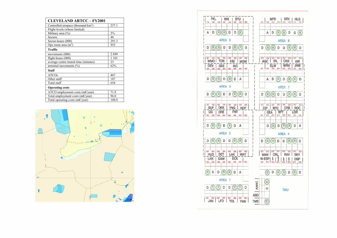
CLEVELAND ARTCC � FY2001Controlled airspace (thousand km2) 237.1Flight levels (where limited)Military area (%) 5%Sectors 46Sector-hours (000) 291.3Ops room area (m2) 953Trafficmovements (000) 2 899flight-hours (000) 1 101average centre transit time (minutes) 23terminal movements (%) 62%StaffATCOs 467Other staff 187Total staff 654Operating costsATCO employment costs (m�/year) 71.9Total employment costs (m�/year) 96.0Total operating costs (m�/year) 108.0

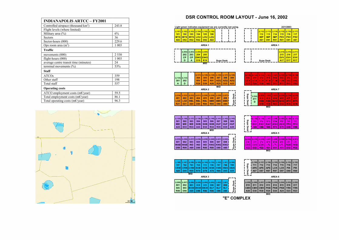
INDIANAPOLIS ARTCC � FY2001Controlled airspace (thousand km2) 243.8Flight levels (where limited)Military area (%) 6%Sectors 36Sector-hours (000) 229.6Ops room area (m2) 1 003Trafficmovements (000) 2 530flight-hours (000) 1 003average centre transit time (minutes) 24terminal movements (%) 53%StaffATCOs 359Other staff 198Total staff 557Operating costsATCO employment costs (m�/year) 59.5Total employment costs (m�/year) 86.1Total operating costs (m�/year) 96.3

DSR CONTROL ROOM LAYOUT - June 16, 2002

Light green indicates equipment we are currently not using.

(L101) 101 MYS A92

(L102) 102 MYS D92

(L103) 103 MYS R92

(L104) 104 LOU R82

(L105) 105 LOU D82

(L106) 106 LOU A82

(L112) 112 IMP A91

(L113) 113 IMP D91

(L114) 114 IMP R91

(L115) 115 PXV R81

(L116) 116 PXV D81

(L117) 117 PXV A81

AREA 1 AREA 1

(L202) 202 CP D

(L203) 203 CP A

(L204) 204

EWO D19

(L205) 205

EWO R19 Supe Desk Supe Desk

(L215) 215 EVV A17

(L216) 216 EVV D17

(L217) 217 EVV R17

MID

(L134) 301 A

(L133) 302 D

(L131) 304 RIV R26

(L130) 305 RIV D26

(L129) 306 RIV A26

(L128) 307 AZQ R25

(L127) 308 AZQ D25

(L126) 309 AZQ A25

(L125) 310 LEX A20

(L124) 311 LEX D20

(L123) 312 LEX R20

(L122) 313 FLM A83

(L121) 314 FLM D83

(L120) 315 FLM R83

(L119) 316 DAC R93

(L118) 317 DAC D93

MIDAREA 2 AREA 7

(L234) 401 LOZ R21

(L233) 402 LOZ D21

(L232) 403 RBL A84

(L231) 404 RBL D84

(L230) 405 RBL R84

(L229) 406 SME R94

(L228) 407 SME D94

(L227) 408 SME A94

(L224) 411 D

(L223) 412 ABB D18

(L222) 413 ABB R18

(L221) 414

MAD R66

(L220) 415

MAD D66

(L219) 416 BTV R76

(L218) 417 BTV D76

MID

(L135) 501 MIE A33

(L136) 502 MIE D33

(L137) 503 MIE R33

(L138) 504 SHB A34

(L139) 505 SHB D34

(L140) 506 SHB R34

(L141) 507 HUF R35

(L142) 508 HUF D35

(L143) 509 HUF A35

(L145) 511 DAY A88

(L146) 512 DAY D88

(L147) 513 DAY R88

(L148) 514 SGH R78

(L149) 515 SGH D78

(L150) 516 FFO D98

(L151) 517 FFO R98

MIDAREA 4 AREA 5

.

(L235) 601

WAB D99

(L236) 602

WAB R99

(L237) 603 IND A89

(L238) 604 IND D89

(L239) 605 IND R89

(L240) 606

KNG R80

(L241) 607

KNG D80

(L242) 608

KNG A80

(L244) 610 CVG A22

(L245) 611 CVG D22

(L246) 612 CVG R22

(L247) 613 LTL R31

(L248) 614 LTL D31

(L249) 615 LTL A31

(L250) 616

ROD D32

(L251) 617

ROD R32

MID

(L168) 701

CRW A85

(L167) 702

CRW D85

(L166) 703

CRW R85

(L165) 704

BOB R79

(L164) 705

BOB D79

(L163) 706

BOB A79

(L162) 707 HNN R95

(L161) 708 HNN D95

(L160) 709 HNN A95

(L158) 711 APE A87

(L157) 712 APE D87

(L156) 713 APE R87

(L155) 714 LCK R97

(L154) 715 LCK D97

(L153) 716 PIK D69

(L152) 717 PIK R69

MIDAREA 3 AREA 6

(L268) 801 SKI R90

(L267) 802 SKI D90

(L266) 803

BKW A86

(L265) 804

BKW D86

(L264) 805

BKW R86

(L263) 806 BLF R96

(L262) 807 BLF D96

(L261) 808 BLF A96

(L259) 810

CMH A30

(L258) 811

CMH D30

(L257) 812

CMH R30

(L256) 813 PKB R24

(L255) 814 PKB D24

(L254) 815 PKB A24

(L253) 816 YRK D23

(L252) 817 YRK R23

MID

"E" COMPLEX

2/21/2003

Supe Desk

Supe

Des

kSu

pe D

esk Supe D

eskSupe D

esk

Supe

Des

k

Report commissioned by the EUROCONTROLPerformance Review Commission

A comparison of performancein selected US and European

En-route Centres

May 2003

Comparison of perform

ance in selected US and European En-route CentresFor any further information please contact:Performance Review Unit, 96 Rue de la Fusée, B-1130 Brussels, Belgium

Tel: + 32 2 729 3956Fax: + 32 2 729 9108

[email protected]://www.eurocontrol.int/prc

PRC2_x 9/05/03 11:51 Page 3

Documents

A comparison of perfromance in selected US and European … · Jim RIES (FAA) Bernd SCHUH (DFS) Riccardo SPADONI (ENAV) Peter TULLETT (NATS) Frans VAN GYSEGEM (Maastricht) Table of