A Comparison of k-NN Methods for Time Series Classi cation

A Comparison of k-NN Methods for Time SeriesClassification and Regression

Vivek Mahato, Martin O’Reilly, and Padraig Cunningham

School of Computer ScienceUniversity College Dublin

Dublin 4, [email protected], [email protected],

[email protected]

Abstract. Interpretability is as important in data analytics on time se-ries data as in other areas of analytics. For this reason, k-Nearest Neigh-bour methods have an important part to play; however coming up witheffective similarity/distance measures is not straightforward given thenature of time series data. In this paper we survey the state-of-the-artdistance measures used for time series analysis and evaluate their effec-tiveness on sample regression and classification tasks. In some circum-stances, a ‘global’ method such as Dynamic Time Warping is effective,whereas for other datasets ‘feature-based’ methods work better.

Keywords: Regression, Classification, Time Series Data

1 Introduction

k-Nearest Neighbour (k-NN) methods have a special status in data analyticsbecause of the importance of explanation and insight. Because k-NN methodsare transparent they produce models that are interpretable. This is also true intime series analysis [9] where side-by-side comparisons of time series can revealsimilarities and differences between process. However, when using k-NN methodsfor time series analysis there is the added challenge of coming up with measuresthat truly capturing the similarity between time series. Two time series mightstill be similar if one is stretched or displaced in time with respect to the other.It may also be the case that similarity depends on short or even tiny signaturesin the time series.

In this paper we provide a short survey of recent methods that address thesechallenges. The methods we consider are:

– Dynamic Time Warping (DTW): Because two time series may be fun-damentally similar but offset or slightly distorted, DTW allows the time axisto be warped to identify underlying similarities [8].

– Symbolic Aggregate Approximation (SAX): The idea with SAX isto discretize the time series so that it can be represented as a sequence ofsymbols [10]. This allows the panoply of data mining methods for sequencesto be applied on the sequence representation of the time series.

2 Vivek Mahato, Martin O’Reilly, and Padraig Cunningham

– Symbolic Fourier Approximation (SFA): SFA is like SAX except thesequence representation is produced from a discrete Fourier transform rep-resentation of the signal rather than a discretization of the signal itself. SoSFA is a frequency domain rather than a time domain representation of thesignal [12].

These three methods are described in detail in the next section. Then anevaluation of the performance of these methods on time series classification andregression tasks is presented in section 3. The evaluation also covers the thornyissue of parameter selection associated with these methods.

2 State-of-the-art Methods

In this section, we discuss the three methods (DTW, SAX, and SFA) coveredin our analysis. The three methods we consider, all require parameter tuning. Ahold-out test strategy is emplyed, where all parameter tuning is done throughcross-validation on the training set before testing on the hold-out set. The pa-rameters chosen are also presented in this section.

2.1 Dynamic Time Warping

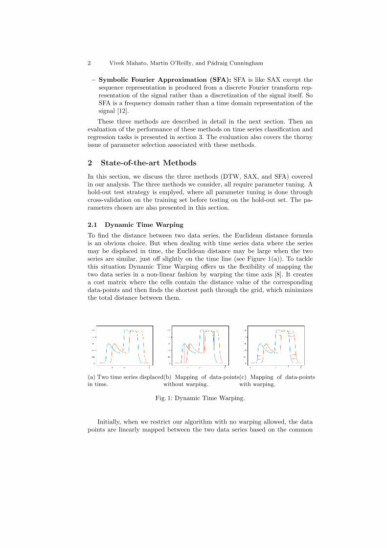
To find the distance between two data series, the Euclidean distance formulais an obvious choice. But when dealing with time series data where the seriesmay be displaced in time, the Euclidean distance may be large when the twoseries are similar, just off slightly on the time line (see Figure 1(a)). To tacklethis situation Dynamic Time Warping offers us the flexibility of mapping thetwo data series in a non-linear fashion by warping the time axis [8]. It createsa cost matrix where the cells contain the distance value of the correspondingdata-points and then finds the shortest path through the grid, which minimizesthe total distance between them.

(a) Two time series displacedin time.

(b) Mapping of data-pointswithout warping.

(c) Mapping of data-pointswith warping.

Fig. 1: Dynamic Time Warping.

Initially, when we restrict our algorithm with no warping allowed, the datapoints are linearly mapped between the two data series based on the common

Dynamic Time Warping in Time Series Regression 3

time axis value. As seen in Figure 1(b), the algorithm does a poor job of match-ing the time series. But when we grant the DTW algorithm the flexibility ofconsidering a warping window, the algorithm performs remarkably when map-ping the data-points following the trend of the time series data, which can bevisualized in Figure 1(c).

2.2 Symbolic Aggregate Approximation

Several symbolic representations of a time series data have been developed inrecent decades with the objective of bringing the power of text processing al-gorithms to bear on time series problems. Keogh et al. provide an overview ofthese methods in their 2003 paper [10].

Symbolic Aggregate Approximation (SAX) is one such algorithm that achievesdimensionality and numerosity reduction and provides a distance measure thatis a lower bound on corresponding distance measures on the orignal series [10].In this case numerosity reduction refers to a more compact representation of theoriginal data.

Piecewise Aggregate Approximation SAX uses Piecewise Aggregate Ap-proximation (PAA) in its algorithm for dimensionality reduction. The funda-mental idea behind the algorithm is to reduce the dimensionality of a time seriesby slicing it into equal-sized fragments which are then represented by the averageof the values in the fragment.

PAA approximates a time seriesX of length n into vector X = (x1, x2, ..., xm)of any arbitrary length m 6 n, where each of xi is computed as follows:

xi =m

n

nm i∑

j= nm (i−1)+1

xj (1)

This simply means that in order to reduce the size from n to m, the original timeseries is first divided into m fragments of equal size and then the mean values foreach of these fragments are computed. The series constructed from these meanvalues is the PAA approximation of the original time series. There are two casesworth noting when using PAA. When m = n the transformed representationis alike to the original input, and when m = 1 the transformed representationis just the mean of the original series [7]. Before the transformation of originaldata into the PAA representation, SAX also normalizes each of the time seriesto have a mean of zero and a standard deviation of one, given the difficulty ofcomparing time series of different scales [10, 6].

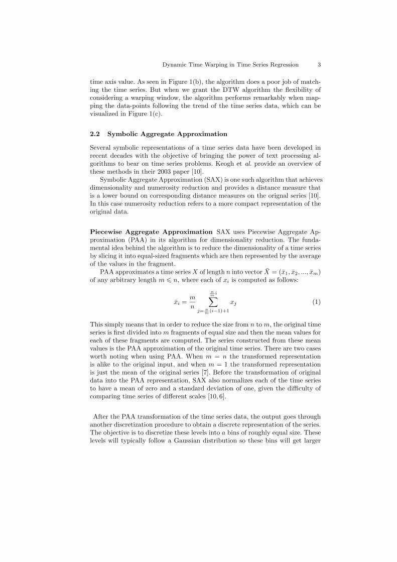
After the PAA transformation of the time series data, the output goes throughanother discretization procedure to obtain a discrete representation of the series.The objective is to discretize these levels into a bins of roughly equal size. Theselevels will typically follow a Gaussian distribution so these bins will get larger


(a) Raw time series data. (b) Time series after PAA di-mensionality reduction.

(c) Mapping of discretizedbins to symbols in SAX.

Fig. 2: Symbolic Aggregate Approximation.

away from the mean. The breakpoints separating these discretized bins form asorted list B = β1, ..., βa−1, such that the area under a N(0, 1) Gaussian curvefrom βi to βi+1 = 1

a . β0 and βa are defined as −∞ and ∞ respectively [10].When all the breakpoints are computed, the original time series is discretized

as follows. First, the PAA transformation of the time series is performed. Theneach of the PAA coefficients less than the smallest breakpoint β1 is mappedto the symbol s1, and all coefficients between breakpoints β1 and β2 (secondsmallest breakpoint) are mapped to the symbol s2, and so on, until the lastPAA coefficient gets mapped. Here, s1 and s2 belongs to a set of symbols S =(s1, s2, ..., sm) to which the time series is mapped by SAX, where m is the sizeof symbol pool.

SAX also has a sliding window implemented in its algorithm, the size ofwhich can be adjusted. It extracts the symbols present in that window frameand creates a word, which is just the concatenated sequence of symbols in thatframe. This sliding window is then shifted to the right and another word isextracted corresponding to the new frame. This goes on until the window hitsthe end of the time series, and we get a “bag-of-words” representing that timeseries.

Once the data is converted to this symbolic representation, one can use thisbag-of-words representation for calculating the distance between two time seriesusing a string distance metric such as Levenshtein distance [15].

2.3 Symbolic Fourier Approximation

SFA was introduced by Schafer et al. in 2012 as an alternative method to SAXbuilt upon the idea of dimensionality reduction by symbolic representation. Un-like SAX which works on the time domain, SFA works on the frequency do-main. In the frequency domain, each dimension contains approximate informa-tion about the whole time series. By increasing the dimensionality one can adddetail, thus improving the overall quality of the approximation. In the time do-main, we have to decide on a length of the approximation in advance and a prefixof this length only represents a subset of the time series [12].


Discrete Fourier Transform In contrast to SAX which uses PAA as its di-mensionality reduction technique SFA, focusing on the frequency domain, usesthe Discrete Fourier Transform (DFT). DFT is the equivalent of the continu-ous Fourier Transform for signals known only at N instants by sample times T ,which is a finite series of data.

Let X(t) be the continuous signal which is the source of the data. Let Nsamples be denoted x[0], x[1], ..., x[N − 1]. The Fourier Transform of the originalsignal, X(t), would be:

F (ωk) ,N−1∑n=0

x(tn)e−jωktn , k = 0, 1, 2, ..., N − 1 (2)

Simply stated, DFT analyzes a time domain signal x(n) to determine thesignal’s frequency content X[k]. This is achieved by comparing x[n] against sig-nals known as sinusoidal basis functions, using correlation. The first few basisfunctions correspond to gradually changing regions and describe the coarse dis-tribution, while later basis functions describe rapid changes like gaps or noise.Thus employing only the first few basis functions yields a good approximationof the time series[12].

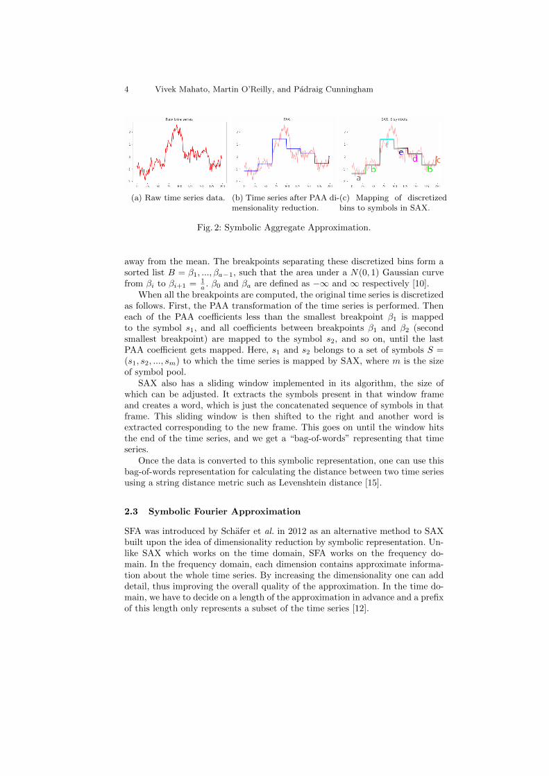
The DFT Approximation is a part of the preprocessing step of SFA algo-rithm, where all time series data are approximated by computing DFT coeffi-cients. When all these DFT coefficients are calculated, multiple discretisationsare determined from all these DFT approximations using Multiple CoefficientBinning (MCB) as shown in Figure 3. MCB helps in mapping the coefficientsto their symbols, and concatenates it to form an SFA word. Thus, this convertsthe time series into its symbolic representation.

Fig. 3: Symbolic Fourier Approximation


As in SAX, there is a sliding window present here which serves the samepurpose of extracting a word representing the data in that frame. Thus, theoutput of SFA for a given source time series is a bag-of-words symbolicallyrepresenting the entire series in lower dimension.

3 Evaluation

When it comes to distance measures, Euclidean distance is a popular choice. Itis easily implemented and has linear time complexity. Moreover, it is parameter-free, and is competitive against more complex approaches, notably when workingon a large dataset. Nevertheless, Euclidean distance is very sensitive to noise anddata being out of phase or warped in time, because of fixed mapping of the pointsof two time series[3].

Another distance measure worth considering is the Levenshtein distance, alsopopularly known as Edit distance, when working on the string or symbolic rep-resentation of the time series. Edit distance measures the distance between twostrings, by computing the number of edits (insertion, deletion or substitution)required to match the strings. The Edit Distance on Real sequences (EDR)[1]and/or with real penalties has been shown to be very effective in time seriesclassification and regression[3].

The Wagner-Fischer algorithm [14] has been shown to be an effective methodfor modelling penalties. It allows for different penalties for insertion, deletionand substitution and for distances within the alphabet to be included in thepenalty score. For example, the basic implementation of Edit distance measuresthe distance between “boat” and “coat” as 1, and the distance between “coat”and “goat” is also computed as 1, because these strings are only 1 edit away.Whereas, the Wagner-Fischer algorithm with our assigned penalties, measuresthe distance between “coat” and “goat” as 4 because ‘g’ is 4 step away from ‘c’in the alphabet.

We compare the three methods (DTW, SAX and SFA) used in time seriesclassification or regression in a k-Nearest Neighbour model against the baselinesof k-NN with Euclidean distance, and random 5-NN. Note that, SAX and SFAproduces a symbolic representation of the time series, so we use EDR and WFas the underlying distance metric.

The evaluation of these methods was conducted on three separate datasets(details below). One of the datasets contains ordered classes so it is included inboth the regression and classification evaluations.

3.1 The Data

In the evaluation we consider one classification and two regression problems.

– Proximal Phalanx TW This is one of the standard datasets from the UCRcollection [2]. It is normally considered a classification task where the classesare ordered age categories but it is also treated as a regression problem here.


– Jump Height It is a jump exercise dataset where the time series was cap-tured using a Shimmer sensor and the target variable is jump height.

– Jump Class This is a classification problem that is a superset of the JumpHeight dataset. It contains three classes, one “correct” class (the JumpHeight samples) and two incorrect classes.

Jumping Data The Jump Height and Jump Class datasets come from the samestudy. Ten participants (3 females, 7 males, age: 26.6 ±2.2, weight: 80.1±7.4 kg, height: 1.8±0.1 m) were recruited for this case-study. The Human ResearchEthics Committee at University College Dublin approved the study protocoland written informed consent was obtained from all participants before testing.Participants did not have a current or recent musculoskeletal injury that wouldimpair performance of Countermovement Jumps (CMJs) . Participants wereequipped with a Shimmer 3 inertial measurement unit (IMU) 1 on their dominantfoot. The IMU was configured to stream wide-range, tri-axial accelerometer data(±16 g) at 1024 Hz. AMTI Force-plate data 2 was also collected concurrentlyat 1000 Hz. This was used as a gold-standard tool to derive time in the air foreach jump [4]. Each participant completed 20 CMJs with acceptable form and40 with incorrect form (2 categories). The resulting data set consisted of 600 filesof IMU data, 200 with acceptable form. This gives us a three class classificationproblem (600 samples) and a regression problem (200 samples).

The length of the IMU signals in each file ranged from 1231 to 6710 sam-ples. The time-series used was the acceleration magnitude, derived from theaccelerometer x, y and z signals whereby:

Am =√A2

x +A2y +A2

z

The target variable for the regression problem was time in the air in seconds,derived from the gold-standard force-plate data.

Note: Each sample in the datasets mentioned above consists of a single uni-variate time-series on which the models are trained to predict its target label.The unequal length of time-series was tackled by padding with 0’s at the endof the shorter time-series when a pairwise distance was computed, between twotime-series.

3.2 Parameter Selection

Parameter selection can have a significant impact on performance in MachineLearning and this is particularly true for the algorithms considered here. Hereis a brief account of the parameter selection required for each of the methods.

1 http://www.shimmersensing.com/products/shimmer3-imu-sensor2 https://www.amti.biz


DTW As mentioned, DTW gives the flexibility of mapping two time-seriesdata warped in time in a non-linear fashion, with the help of a warping window.Thus, finding an optimal warping window is crucial for the algorithm. Aftercross-validation on the training data, we set the warping window for Proximal-PhalanxTW, JumpingHeight and Jumping datasets to be 2, 26 and 26 respec-tively.

SAX The implementation of SAX [13] employed in this study has a large pa-rameter space, consisting of five different parameters in total. The following arethe parameters available:

1. Window size: The window size refers to the sliding window size w, whichis the length of the frame on the x-axis. As SAX only considers the PAAcoefficients present in the frame to map to symbols and create a SAX word,the window size plays a crucial role. The window size also affects the lengthof the words in the bag. It was set to 15, 40, and 30 for ProximalPhalanx,JumpHeight, and Jumping respectively.

2. PAA size: This parameter adjusts the number of discretized bins of equal-width on the x-axis. The mean of the data-points in each bin is calculatedto compute the PAA coefficient. As PAA is the underlying dimensionalityreduction method used in SAX, this parameter also requires a precise ad-justment to describe the time-series well, with minimal loss of information.The PAA size was also set to be 15, 40 and 30 respectively for the threedatasets.

3. Alphabet size: The discretization performed on the y-axis is governed by thisparameter. Therefore, it is the number of bins of equal-probability denotedby a symbol from the Symbolic pool. For example, an alphabet size of 3creates three levels or bins on the y-axis, and each of those bins can berepresented by symbols, ‘a’,‘b’ and ‘c’ respectively. It was set to of 5, 20 and20 respectively.

4. NR Strategy: This parameter determines the numerosity reduction strategyapplied to the converted SAX words to eliminate duplicate data. The threestrategies which can be selected are “none”, “exact” and “mindist”. In allcases “none” was used.

5. Z-threshold: The time-series passed to PAA is normalised using z-normal-isation. This parameter helps to adjust the threshold value of z-normalisationstep in the algorithm. On preliminary inspection which resulted in 0.1 to bean optimum value for this parameter over the datasets, we set it to 0.1 forall SAX models in our experiments.

Note that as the parameter search space is high, we opted on setting the NR-strategy and z-threshold to be static on an optimum value following our pre-liminary experiments. The most influential parameters to this model are slidingwindow size, PAA size and alphabet size.


SFA The implementation of SFA [5] employed is a Python port of the originalproject[11]. There are five parameters to estimate which like in SAX, results ina large parameter space.

1. Window-size: As in SAX, the window size here also refers to the slidingwindow size w. The DFT coefficients present are mapped to symbols to createan SFA word. It was set to 5, 45, and 45 for ProximalPhalanx, JumpHeight,and Jumping datasets respectively.

2. Word-length: This parameter controls the length of the words in the bag-of-words. This parameter was set to be the same as the sliding-window size,i.e. 5, 45, and 45.

3. Alphabet-size: This serves the same purpose as in SAX. It is the quantizationover the y-axis. This parameter was set to be 5, 20, and 20 for the threedatasets.

4. Norm-mean: The data can be normalised to the signal mean or left unnor-malised.

5. Lower-bounding: SFA uses lower-bounding distance measure during discretiza-tion with MCB [12] to have a reduced but still effective search space. It canbe set to True or False, depending on the application if this feature is wanted.

The parameter search space is high as in SAX, we opted on setting the Norm-mean and Lower-bounding parameters to be True following our preliminary ex-periments. The most influential parameters to this model are sliding windowsize, word length and alphabet size.

Note k-NN has only one parameter, the neighbourhood size (k). We chose togo with the best k value for each model by measuring its performance by 10-foldcross-validation on the train set.

3.3 Model Performance

This section deals with the performance of the three methods, DTW, SAX, andSFA against two baseline models, Euclidean distance (ED) and Random 5-NN.For SAX and SFA we consider both EDR and WF string distance measures sowe evaluate five candidates against two baselines.

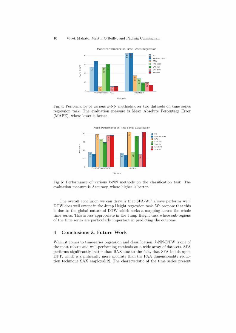
Figure 4 illustrates the performance of the models on time-series regressiontask over two datasets. Mean Absolute Percentage Error (MAPE) metric wasemployed to evaluate the performance, where a lower MAPE score signifies betterperformance. While DTW does not perform well on the Jump Height task it isthe best model on the Proximal Phalanx task. Here, we can see that SFA withWF is consistent than the other models, showing robustness.

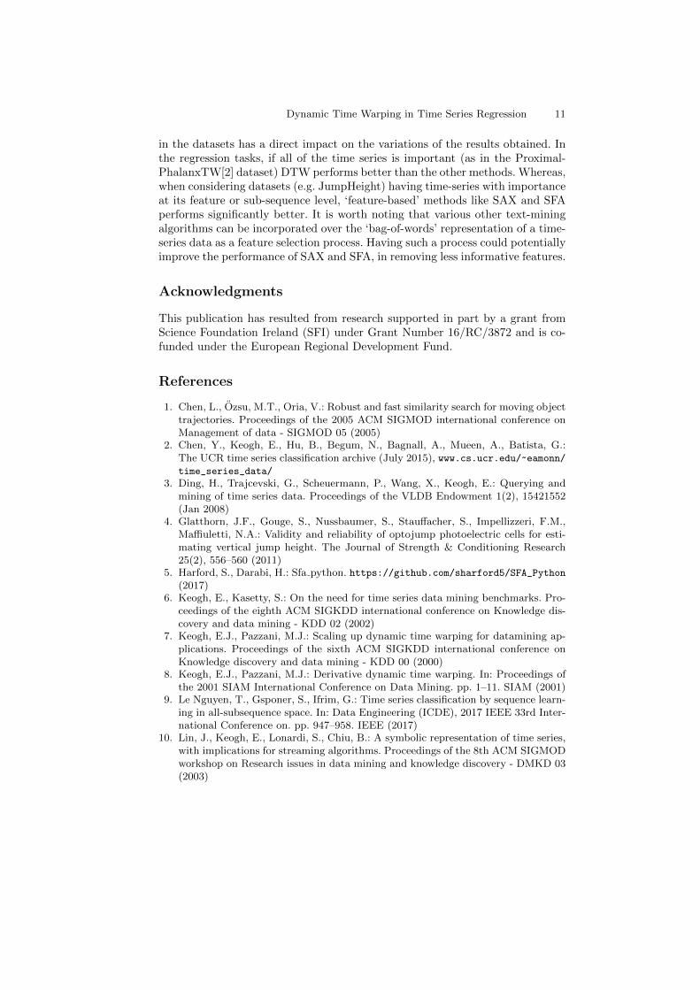
Figure 5 shows the performance on the classification tasks. Here the measureis classification accuracy so higher is better. When it comes to time-series clas-sification we can see DTW performed best, and SFA-WF comes a close second.The WF string distance measure shows a significant impact when working onthe Jumping dataset.


Fig. 4: Performance of various k-NN methods over two datasets on time seriesregression task. The evaluation measure is Mean Absolute Percentage Error(MAPE), where lower is better.

Fig. 5: Performance of various k-NN methods on the classification task. Theevaluation measure is Accuracy, where higher is better.

One overall conclusion we can draw is that SFA-WF always performs well.DTW does well except in the Jump Height regression task. We propose that thisis due to the global nature of DTW which seeks a mapping across the wholetime series. This is less appropriate in the Jump Height task where sub-regionsof the time series are particularly important in predicting the outcome.

4 Conclusions & Future Work

When it comes to time-series regression and classification, k-NN-DTW is one ofthe most robust and well-performing methods on a wide array of datasets. SFAperforms significantly better than SAX due to the fact, that SFA builds uponDFT, which is significantly more accurate than the PAA dimensionality reduc-tion technique SAX employs[12]. The characteristic of the time series present


in the datasets has a direct impact on the variations of the results obtained. Inthe regression tasks, if all of the time series is important (as in the Proximal-PhalanxTW[2] dataset) DTW performs better than the other methods. Whereas,when considering datasets (e.g. JumpHeight) having time-series with importanceat its feature or sub-sequence level, ‘feature-based’ methods like SAX and SFAperforms significantly better. It is worth noting that various other text-miningalgorithms can be incorporated over the ‘bag-of-words’ representation of a time-series data as a feature selection process. Having such a process could potentiallyimprove the performance of SAX and SFA, in removing less informative features.

Acknowledgments

This publication has resulted from research supported in part by a grant fromScience Foundation Ireland (SFI) under Grant Number 16/RC/3872 and is co-funded under the European Regional Development Fund.

References

1. Chen, L., Ozsu, M.T., Oria, V.: Robust and fast similarity search for moving objecttrajectories. Proceedings of the 2005 ACM SIGMOD international conference onManagement of data - SIGMOD 05 (2005)

2. Chen, Y., Keogh, E., Hu, B., Begum, N., Bagnall, A., Mueen, A., Batista, G.:The UCR time series classification archive (July 2015), www.cs.ucr.edu/~eamonn/time_series_data/

3. Ding, H., Trajcevski, G., Scheuermann, P., Wang, X., Keogh, E.: Querying andmining of time series data. Proceedings of the VLDB Endowment 1(2), 15421552(Jan 2008)

4. Glatthorn, J.F., Gouge, S., Nussbaumer, S., Stauffacher, S., Impellizzeri, F.M.,Maffiuletti, N.A.: Validity and reliability of optojump photoelectric cells for esti-mating vertical jump height. The Journal of Strength & Conditioning Research25(2), 556–560 (2011)

5. Harford, S., Darabi, H.: Sfa python. https://github.com/sharford5/SFA_Python(2017)

6. Keogh, E., Kasetty, S.: On the need for time series data mining benchmarks. Pro-ceedings of the eighth ACM SIGKDD international conference on Knowledge dis-covery and data mining - KDD 02 (2002)

7. Keogh, E.J., Pazzani, M.J.: Scaling up dynamic time warping for datamining ap-plications. Proceedings of the sixth ACM SIGKDD international conference onKnowledge discovery and data mining - KDD 00 (2000)

8. Keogh, E.J., Pazzani, M.J.: Derivative dynamic time warping. In: Proceedings ofthe 2001 SIAM International Conference on Data Mining. pp. 1–11. SIAM (2001)

9. Le Nguyen, T., Gsponer, S., Ifrim, G.: Time series classification by sequence learn-ing in all-subsequence space. In: Data Engineering (ICDE), 2017 IEEE 33rd Inter-national Conference on. pp. 947–958. IEEE (2017)

10. Lin, J., Keogh, E., Lonardi, S., Chiu, B.: A symbolic representation of time series,with implications for streaming algorithms. Proceedings of the 8th ACM SIGMODworkshop on Research issues in data mining and knowledge discovery - DMKD 03(2003)


11. Schafer, P.: Sfa. https://github.com/patrickzib/SFA (2015)12. Schafer, P., Hogqvist, M.: SFA: a symbolic fourier approximation and index for

similarity search in high dimensional datasets. In: Proceedings of the 15th Interna-tional Conference on Extending Database Technology. pp. 516–527. ACM (2012)

13. Senin, P., Lin, J., Wang, X., Oates, T., Gandhi, S., Boedihardjo, A.P., Chen, C.,Frankenstein, S., Lerner, M.: Grammarviz 2.0: A tool for grammar-based patterndiscovery in time series. In: Calders, T., Esposito, F., Hullermeier, E., Meo, R.(eds.) Machine Learning and Knowledge Discovery in Databases. pp. 468–472.Springer Berlin Heidelberg, Berlin, Heidelberg (2014)

14. Wagner, R.A., Fischer, M.J.: The string-to-string correction problem. Journal ofthe ACM 21(1), 168173 (Jan 1974)

15. Yujian, L., Bo, L.: A normalized levenshtein distance metric. IEEE transactionson pattern analysis and machine intelligence 29(6), 1091–1095 (2007)

Documents

A Comparison of k-NN Methods for Time Series Classi cation