Embed Size (px)
Citation preview
A comparison of friction piles bearing capacity based on theoretical and empirical mathematical models
Ermias Hailu Mijena
Geotechnics and Geohazards
Supervisor: Lars Olav Grande, BAT
Department of Civil and Transport Engineering
Submission date: July 2012
Norwegian University of Science and Technology

I
Key words: pile, bearing capacity, pile load test, analyses
(Signature)
NORGES TEKNISK- NATURVITENSKAPELIGE UNIVERSITET INSTITUTT FOR BYGG, ANLEGG OG TRANSPORT
Report Title: A comparison of friction piles bearing capacity based on theoretical and empirical mathematical models.
Date: July 09, 2012 Number of pages (including appendices): 116
Masteroppgave X Projektoppgave
Name: Ermias Hailu Mijena
Professors in charge/Supervisor: Lars Grande
Other external professional /Supervisors: Dr. Tewodros Tefera, Frode Oset and Grete Trevdt
Abstract
One can find in literature lots of different models to predict axial capacity of piles .This study has been carried out to compare some selected empirical (semi-empirical) and theoretical models used in Norway or internationally. The comparisons were made among the various models with respect to the static load test result, which is widely believed to be providing a reliable pile capacity. The study has been undergone based on the data obtained in the bridge project over the Drammen Selva river in the city of Drammen in Norway. In this study, I have included four calculation models, namely the Janbu theoretical models (derived based on plasticity theories and earth pressure approach), the Norwegian Pile Guideline (peleveiledningen (2005)), API RP 2A LRFD (2007), NGI-99 methods. The Norwegian Pile Guideline (2005) is sort of mixed empirical and theoretical approach. The last two are purely empirical.
Recent literature on set up effect were also included in this study and the increase in capacity with time was also accessed in both using a prediction model and static load test result which was performed in various time intervals.
Additionally, a back calculation of parameters was also performed in the study based on the static load test results, for a possible use in design of neighboring piles showing similar soil type and soil parameters. We should be aware that the findings of this study is considered to be of limited nature and should not be generalized.

II
ACKNOWLEDGMENTS
I would like to thank Frode Oset from Norwegian Public Road Administration (NPRA) for making this thesis title available for masters’ students to work on it. In particular, I would like to thank my supervisor Dr. Tewodros Tefera from Norwegian Public Road Administration (NPRA) for providing me the opportunity to work on this project, providing me material support and his continuous encouragement and guidance throughout the course of this project.
Moreover, I would also like to thank Professor Lars Grande from Norwegian University of Science and Technology (NTNU) for all kind of tireless help they gave me which I consider has an immense contribution for the success of the project.
My deepest gratitude also extends to Grete Trevdt from Norwegian Public Road Administration (NPRA) for providing me material support which is vital for the success of the project work.
Special thanks to my families back home for worrying about the progress of my study and my well-being in a foreign country.
Last and not the least, I would like to thank all my friends and roommates living in the Moholt Studentby for being beside me and giving me their continuous moral support.
III
Contents
ACKNOWLEDGMENTS ....................................................................................................................... II
LIST OF SYMBOLS............................................................................................................................. VII
LIST OF FIGURES ................................................................................................................................ IX
LIST OF TABLES ................................................................................................................................ XII
1 INTRODUCTION ................................................................................................................................ 1
1.1 Background ................................................................................................................................... 1
1.2 Scope and objective of the work ................................................................................................... 1
1.3 Outline of the work ........................................................................................................................ 2
1.4 Methodology ................................................................................................................................ 2
1.5 Delimitation ................................................................................................................................... 2
2 PILE TYPES ........................................................................................................................................ 3
2.1 Nature of load support ................................................................................................................... 3
2.1.1 Friction piles ........................................................................................................................... 3
2.1.2 End bearing piles .................................................................................................................... 3
2.2 Displacement nature ...................................................................................................................... 4
2.2.1 Displacement piles.................................................................................................................. 4
2.2.2 Partial-displacement piles ....................................................................................................... 4
2.2.3 Non-displacement piles .......................................................................................................... 4
2.3 Material composition ..................................................................................................................... 4
2.3.1 Timber Piles ........................................................................................................................... 4
2.3.2 Concrete piles ......................................................................................................................... 5
2.3.3 Steel Piles ............................................................................................................................... 6
3 SOIL PARAMETERS FOR PILE ANALYSES AND DESIGN ........................................................ 7
3.1 Scope, objectives and extent of the soil investigation ................................................................... 7
3.2 Various soil investigation and testing methods ............................................................................. 7
3.2.1 Boring techniques ................................................................................................................... 7
3.2.2 Soil sampling and laboratory testing ...................................................................................... 7
3.2.3 Field testing ............................................................................................................................ 9
3.2.4 Groundwater level measurement .......................................................................................... 12
3.3 Design parameters ....................................................................................................................... 13
IV
3.3.1 Strength parameters .............................................................................................................. 13
3.3.2 Soil pile adhesion ................................................................................................................. 14
3.3.3 Elastic soil parameters .......................................................................................................... 14
4 STATIC PILE CAPACITY ................................................................................................................ 15
4.1 Empirical Methods ...................................................................................................................... 16
4.1.1 Method based on Cone penetration test (CPT) ..................................................................... 16
4.1.2 Method based on Standard penetration test (SPT) ............................................................... 17
4.1.3 Axial pile capacity in clay using various pile design practices ............................................ 18
4.1.4 Axial capacity in sand using the various pile design practices ............................................. 24
4.2 Theoretical method ...................................................................................................................... 28
4.2.1 Short term capacity ............................................................................................................... 28
4.2.2 Long term capacity ............................................................................................................... 30
4.3 Effect of time on pile capacity..................................................................................................... 34
4.4 Effect of plugging on pile capacity ............................................................................................. 37
4.5 Build-up/ drop-off in bearing capacity in layered soils ............................................................... 38
5 PILE DYNAMICS AND PILE LOAD TESTS ................................................................................. 40
5.1 Pile installation ............................................................................................................................ 40
5.2 Pile driving formulas ................................................................................................................... 41
5.3 Wave equation analysis ............................................................................................................... 43
5.4 Pile Load Tests ............................................................................................................................ 45
5.4.1 Static pile load test................................................................................................................ 45
5.4.2 Testing methods ................................................................................................................... 46
5.4.3 Interpretation of the load test ................................................................................................ 47
5.5 Pile driving stresses ..................................................................................................................... 50
6 CASE STUDY ................................................................................................................................... 51
6.1 Background of the study .............................................................................................................. 51
6.2 Soil condition of the area ............................................................................................................. 54
6.3 Soil Parameters ............................................................................................................................ 54
6.3.1 Soil parameters at axis 16 ..................................................................................................... 55
6.3.2 Soil parameters at axis 25 ..................................................................................................... 56
6.4 Pile parameters ............................................................................................................................ 57
6.5 Load tests ..................................................................................................................................... 57
7 ANALYSES AND RESULTS ........................................................................................................... 59
7.1 Results of the analyses ................................................................................................................ 59
V
7.1.1 Results of the analyses using empirical and theoretical methods for axis 16P2................... 59
7.1.2 Results of the analyses using empirical and theoretical methods for axis 16P2................... 60
7.1.3 Results of the analyses using empirical and theoretical methods for axis 25P1................... 61
7.1.4 Results of the analyses using empirical and theoretical methods for axis 25P2................... 62
7.2 Interpretation of the load test ....................................................................................................... 63
7.2.1 Interpretation of the load test at axis 16 P1 .......................................................................... 64
7.2.2 Interpretation of the load test at axis 16 P2 .......................................................................... 67
7.2.3 Interpretation of the load test at axis 25 P1 .......................................................................... 70
7.2.4 Interpretation of the load test at axis 25 P2 .......................................................................... 72
7.3 Comparison of the ultimate pile bearing capacity from the various empirical and theoretical methods with that of the static load test result .................................................................................. 75
7.3.1 Comparison of the various empirical and theoretical methods with the static load test result at axis 16P1 ................................................................................................................................... 76
7.3.2 Comparison of the various empirical and theoretical methods with the static load test result at axis 16P2 ................................................................................................................................... 77
7.3.3 Comparison of the various empirical and theoretical methods with the static load test result at axis 25P1 ................................................................................................................................... 78
7.4.4 Comparison of the various empirical and theoretical methods with the static load test result at axis 25P2 ................................................................................................................................... 79
7.4 Comparison of ultimate pile bearing capacity determined by PDA, CAPWAP and static load test ........................................................................................................................................................... 80
7.5 Increase in pile bearing capacity with time ................................................................................. 83
7.6 Back calculation of Janbu theoretical parameters based on the static load test results ............... 85
8 CONCLUSIONS AND FUTURE WORK ......................................................................................... 86
REFERENCES ...................................................................................................................................... 87
APPENDIX A ....................................................................................................................................... 89
APPENDIX B...................................................................................................................................... 104
APPENDIX C...................................................................................................................................... 111
VI
LIST OF SYMBOLS 𝛾 unit weight
𝑤 weight of soil
𝑤𝑤 weight of water
𝑤𝑠 weight of solid
𝑣𝑣 volume of void
𝑣𝑠 volume of solid
𝐷𝑟 relative density
𝑒𝑚𝑎𝑥 maximum void ratio
𝑒𝑛 natural void ratio
𝑒𝑚𝑖𝑛 minimum void ratio
𝐼𝑃 plasticity index
𝑤𝐿 liquid limit
𝑤𝑃 plastic limit
𝑂𝐶𝑅 overconsolidation ratio
𝑝𝑐′ preconsolidation pressure
𝑝0′ current overburden pressure
𝑐 cohesion
𝜑(𝛷) friction angle
𝑠𝑢 undrained shear strength
𝜎𝑣′ vertical effective stress
𝑠𝑡 sensativity
𝑆𝑃𝑇 standard penetration test
𝐶𝑃𝑇 cone penetration test
𝑀 oedometer modulus
𝐺 shear modulus
VII
𝑞𝑡 corrected cone resistance
𝑞𝑐 measured cone resistance
𝑞𝑛𝑒𝑡 net tip resistance
𝑓𝑡 corrected sleeve friction
𝑓𝑠 measured sleeve friction
𝑢 pore pressure
𝑁𝐾𝑇 bearing capacity factor
𝑄𝑃 pile tip capacity
𝑄𝑆 pile skin capacity
𝑄𝑢 ultimate pile capacity
𝑄𝑎 allowable pile capacity
𝑞𝑝 unit tip capacity
𝑓𝑠(𝜏𝑠) unit skin friction capacity
𝑁 SPT blow count
𝛼 adhesion coefficient
𝑝0′ effective vertical overburden
𝐿 length of pile
𝑑(𝐵) diameter of pile
𝑞′ effective vertical overburden
𝐾 coefficient of lateral earth pressure
𝛿 friction angle between soil and pile wall
𝑁𝑞 bearing capacity factor
𝑁𝑐 bearing capacity factor
𝜏 shear stress
𝑡 time
𝑟 roughness coefficient
𝑎 attraction
VIII
𝛽(ᴪ) plastification angle
𝑇 dimensionless time factor
𝑐ℎ horizontal coefficient of consolidation
𝑈 degree of consolidation
𝐼𝐹𝑅 incremental filling ratio
𝑃𝐿𝑅 plug length ratio
𝜂 hammer efficiency
𝑤𝑟 ram weight
𝑤𝑝 pile weight
𝑃𝑢 ultimate pile capacity
𝐸ℎ hammer energy
𝑅𝑠 static soil resistance
𝐽 a damping constant
𝑉 instantaneous velocity
𝑓𝑢 tensile stregth
𝑓𝑐 compressive stregth
𝑓𝑦 yield stress
𝑟0 outer pile radius
𝑟𝑝 radius of the plastic zone
𝑟𝑖 inner pile radius
𝐺50 shear modulus at 50% of maximum stress
𝑐𝑢 undrained shear strength
IX
LIST OF FIGURES Figure 2.1 Friction pile ……………………………………………………………………….3 Figure 2.2.End bearing pile …………………………………………………………………..3 Figure 2.3 Timber piles used as foundation in the city of Trondheim……………………….5 Figure 2.4 Concrete piles used as foundation material ……………………………………....6 Figure 3.1Cone penetration test……………………………………………………………....10 Figure 3.2 Bjerrum’s correction factor for vane shear test [After Bjerrum’s (1972) and Ladd et al. (1977)]……………………………………11 Figure 3.3 Reinterpretation of Bjerrum chart by Aas et al…………………………………..12 Figure 4.1 Relationship between the adhesion factor and undrained shear strength………..18 Figure 4.2The dependent of λ coefficient on pile penetration. Data plotted and depth converted to meters by author from Vijayvergiya and Focht (1972)…………….................19 Figure 4.3 Side friction according to peleveiledningen 1991 (after Gunnar Aas)…………..21 Figure 4.4 Comparison between α − su
σ′vo� relationsfrom new tests and load test data from API data base…………………………………………………………………………………22 Figure 4.5 Comparison between NGI-99 and API-87 α -values………………………….....23 Figure 4.6 Normalised side friction for piles installed in normally consolidated clay……....24 Figure 4.7 Side friction factor and bearing capacity factor in sand according to peleveiledningen 1991………………………………………………………………………..25 Figure 4.8 Recommended parameters according to API-87 for piles in cohesionless siliceous soil………………………………………………………………............................................26 Figure 4.9 Forces on open ended pile………………………………………………………...27 Figure 4.10 Side friction derivation using earth pressure concept …………………………..29 Figure 4.11 Point bearing……………………………………………………………………..29 Figure 4.12 vS vs. tan ρ chart for compressive pile………………………………………...31 Figure 4.13 vS vs. tan ρ chart for piles with negative skin friction ………………………...32 Figure 4.14 𝑁𝑞 vs tan ρ chart for different plastification angles………………………….....33 Figure 4.15 Point bearing capacity factor 𝑁𝑞 vs tan ρ chart …………………..…………….33 Figure 4.16 Changes in pile stress regime over time………………………………………....34 Figure 4.17 Time factors vs. degree of consolidation from linear radial consolidation theory of 1) ∆ui decreases linearly with log (r r0� ), 2) ∆ui decreases linearly with (r r0� ) (based on analytical results presented by Levadoux, 1982 and Chin, 1986)……………………………36 Figure 4.18 Proposed build-up of shaft friction during the re-consolidation phase………….36 Figure 4.19 Definition incremental filling ratio and plug length ratio…………………….....38 Figure 4.20 Build-up/drop-off in end-bearing resistance in layered soils……………………39 Figure 5.1Concrete pile driving in the city of Oslo…………………………………………..41 Figure 5.2 Basic concepts behind derivation of pile driving formula………………………..42 Figure 5.3 Wave equation analyses: Method or representation of pile and other parts of modell. a) Actual, b) as represented (after Smith, 1962)…………………………………......44 Figure 5.4 Typical pile load set up using adjacent piles in group for reaction……………….46 Figure 5.5 Typical pile load set up using adjacent piles in group for reaction……………….47 Figure 5.6 Load test interpretation using Brinch Hansen’s 90% criterion……………………48 Figure 5.7 Load test interpretation using Brinch Hansen’s 80% criterion……………………48 Figure 5.8 Load test interpretation using Davisson’s offset limit method……………………49 Figure 5.9 Load test interpretation using Chin-Kondner method…………………………….49 Figure 5.10 Load test interpretation using De Beer’s method………………………………..50 Figure 6.1 The bridge site…………………………………………………………………….51
X
Figure 6.2 section and plan view of the new bridge project………………………………...53 Figure 6.3 The old and new bridge side by side after completion of the new bridge ………53 Figure 6.4 The old and the new bridge side by side after the pier of the old bridge upgraded to a circular cross section……………………………………………………………………….54 Figure 6.5 Static load test at axis 16………………………………………………………….57 Figure 6.6 Static load test at axis 25…………………………………………………………58 Figure 7.1 Load-movement plot at axis 16 using steel pipe pile of 11m length measured one day after driving……………………………………………………………………………....64 Figure 7.2 Load-movement plot at axis 16 using steel pipe pile of 17m length measured one day after driving……………………………………………………………………………...65 Figure 7.3 Load-movement plot at axis 16 using steel pipe pile of 35m length measured one day after driving……………………………………………………………………………...65 Figure 7.4 Load-movement plot at axis 16 using steel pipe pile of 35m length measured 14 days after driving……………………………………………………………………………..66 Figure 7.5 Load-movement plot at axis 16 using steel pipe pile of 35m length measured 4 months after driving…………………………………………………………………..............66 Figure 7.6 Load-movement plot at axis 16 using HP pile of 11m length measured one day after driving…………………………………………………………………………………...67 Figure 7.7 Load-movement plot at axis 16 using HP pile of 17m length measured one day after driving…………………………………………………………………………………...68 Figure 7.8 Load-movement plot at axis 16 using HP pile of 35m length measured one day after driving…………………………………………………………………………………...68 Figure 7.9 Load-movement plot at axis 16 using HP pile of 35m length measured 14 days after driving…………………………………………………………………..……………...69 Figure 7.10 Load-movement plot at axis 16 using HP pile of 35m length measured 4 months after driving……………………………………………………………………....................69 Figure 7.11 Load-movement plot at axis 25 using steel pipe pile of 15m length measured one day after driving……………………………………………………………………………...70 Figure 7.12 Load-movement plot at axis 25 using steel pipe pile of 25m length measured one day after driving……………………………………………………………………………...71 Figure 7.13 Load-movement plot at axis 25 using steel pipe pile of 25m length measured 14 days after driving………………………………………………………………………….....71 Figure 7.14 Load-movement plot at axis 25 using steel pipe pile of 25m length measured 4 months after driving………………………………………………………………................72 Figure 7.15 Load-movement plot at axis 25 using HP pile of 15m length measured one day after driving…………………………………………………………………………………...73 Figure 7.16 Load-movement plot at axis 25 using HP pile of 25m length measured one day after driving…………………………………………………………………………………...73 Figure 7.17 Load-movement plot at axis 25 using HP pile of 25m length measured 14 days after driving…………………………………………………………………………………...74 Figure 7.18 Load-movement plot at axis 25 using HP pile of 25m length measured 4 months after driving………………………………………………………………………...................74 Figure 7.19 Comparison of the various empirical and theoretical methods with the static load test result at axis 16P1…………………………………………………..................................76 Figure 7.20 Comparison of the various empirical and theoretical methods with the static load test result at axis 16P2…………………………………………………..................................77 Figure 7.21 Comparison of the various empirical and theoretical methods with the static load test result at axis 25P1…………………………………………………..................................78 Figure 7.22 Comparison of the various empirical and theoretical methods with the static load test result at axis 25P2………………………………………………….................................79
XI
Figure 7.23 Increase in pile bearing capacity with time with for axis 16P1…………………84 Figure 7.24 Increase in pile bearing capacity with time with for axis 16P2…………………84
XII
LIST OF TABLES
Table 6.1 soil parameters for the clay at axis 16……………………………………………...55 Table 6.2 soil parameters for the sand at axis 16……………………………………………..55 Table 6.3 CPTU results at axis 16…………………………………………………………….56 Table 6.4 soil parameters for the sand at axis 25……………………………………………..56 Table 6.5 CPTU results at axis 25…………………………………………………………….57 Table 7.1 Pile capacity results using the various empirical and theoretical methods for axis 16P1…………………………………………………………………………………………..59 Table 7.2 bearing capacity factor Nq computed using Janbu, Norwegian Pile Guideline (2005) and API RP 2A LRFD (2007) method………………….........................................................60 Table 7.3 Pile capacity results using the various empirical and theoretical methods for axis 16P2…………………………………………………………………………………………..61 Table 7.4 Pile capacity results using the various empirical and theoretical methods for axis 25P1…………………………………………………………………………………………..62 Table 7.5 Pile capacity results using the various empirical and theoretical methods for axis 25P2…………………………………………………………………………………………..62 Table 7.6 Ultimate pile capacity from the static load test for axis 16P1…………………….67 Table 7.7 Ultimate pile capacity from the static load test for axis 16P2…………………….70 Table 7.8 Ultimate pile capacity from the static load for axis 25P1…………………………72 Table 7.9 Ultimate pile capacity from the static load test for axis 25P2…………………….75 Table 7.10 Comparison of the PDA, CAPWAP and static load test results for pile length 9-11m for axis 16P1…………………………………………………………………………….80 Table 7.11 Comparison of the PDA, CAPWAP and static load test results for pile length 16.1-17m for axis 16P1…………………………………………………………………………….80 Table 7.12 Comparison of the PDA, CAPWAP and static load test results for pile length 33-35m for axis 16P1…………………………………………………………………………….81 Table 7.13 Comparison of the PDA, CAPWAP and static load test results for pile length 9-11m for axis 16P2…………………………………………………………………………….81 Table 7.14 Comparison of the PDA, CAPWAP and static load test results for pile length 15-17m for axis 16P2…………………………………………………………………………….81 Table 7.15 Comparison of the PDA, CAPWAP and static load test results for pile length 34.3-35m for axis 16P2…………………………………………………………………………….82 Table 7.16 Comparison of the PDA, CAPWAP and static load test results for pile length 15m for axis 25P1………………………………………………………………………………….82 Table 7.17 Comparison of the PDA, CAPWAP and static load test results for pile length 23-25m for axis 25P1…………………………………………………………………………….82 Table 7.18 Comparison of the PDA, CAPWAP and static load test results for pile length 13.5-15m for axis 25P2…………………………………………………………………………….83 Table 7.19 Comparison of the PDA, CAPWAP and static load test results for pile length 22-25m for axis 25P2…………………………………………………………………………….83 Table 7.20 Back calculated 𝑠𝑣 and 𝑁𝑞 values……………………………………………….85
[A COMPARISON OF FRICTION PILES BEARING CAPACITY BASED ON THEORETICAL AND EMPIRICAL MATHEMATICAL
MODELS] July 9, 2012
1
1 INTRODUCTION
1.1 Background Piles are structural members that transmit the super structure loads to deep soil layers. They are preferred to be used as a foundation material when shallow foundation is not practical to use it. Piles and pile foundations have been in use since prehistoric times [15].The Roman wooden piles are classic example for this. Today piles can be made of wood, concrete or steel. Pile capacity determination is a difficult thing. A number of different designs practices here in Norway and internationally exist, but seldom have they given the same computed capacity. Especially, determining the skin friction component is not an easy thing since the soil is not intact after the pile is driven and loses its intact engineering property (strength). So far, precise determination of this value has not been possible. Thus today design offices only believe a load test can only give reliable capacity of the pile at the time of test. After installation the design values, i.e. the load carrying capacities of piles are usually verified using different methods such as pile loading test and dynamic analysis. Scientific approaches to pile design have advanced enormously in recent decades and yet, still the most fundamental aspect of pile design - that of estimating capacity –relies heavily upon empirical correlations [17]. The study focuses on some of selected empirical (semi-empirical) and theoretical mathematical models used here in Norway and internationally. In order to compare the various models, a case study was chosen, which a bridge project with construction was began back in 2002 and completed in 2006 and the bridge is located in the city of Drammen over the Dramen Selva river in Norway. During the investigation of the bridge project, both static and dynamic load tests were performed in order to determine the pile capacity. The load tests were performed on single piles at two chosen axis namely, axis 16 and 25 and both closed-ended steel pipe pile and HP pile were load tested. The study focuses only on the capacity of single pile under compressive loading condition for the single piles at axis 16 and axis 25. Of course in reality seldom single piles are used, however, the capacity of group piles entirely depends on the capacity of single pile within a group. It should be noted that the pile group capacity is not the intension of this study.
1.2 Scope and objective of the work The scope of the project work includes
1) Literature survey The focus is to do intensive literature survey about empirical and theoretical based practices. 2) Analysis and evaluation
[A COMPARISON OF FRICTION PILES BEARING CAPACITY BASED ON THEORETICAL AND EMPIRICAL MATHEMATICAL
MODELS] July 9, 2012
2
The focus is to compare the empirical and theoretical based mathematical models with pile load test and dynamic analysis on the selected case study.
1.3 Outline of the work
This thesis consists of 8 chapters and each chapter is described as follows: Chapter 2: Presents the different types of piles which exist today and their classification. Chapter 3: Presents the different soil parameters we use in pile analyses and design and the properties of these parameters. Chapter 4: Presents the different empirical and theoretical static pile capacity equation. It also presents the effect of time and plugging on pile capacity. Chapter 5: Presents pile dynamics, static and dynamic load tests on piles. Chapter 6: Presents a case study which is a case of a bridge project on the Drammen selva river in Drammen, Norway. Chapter 7: Presents the analysis and results obtained for the case study described in chapter 6. Chapter 8: It is the last part of the work which presents conclusions and possible future work.
1.4 Methodology
1) Literature review of various methods of predicting pile capacity 2) Single Pile capacity was computed using the various chosen methods 3) Static load test result was chosen as a reference in comparison 4) Comparisons were made between the various empirical and theoretical methods 5) Back calculation of soil data was performed in order to use for neighboring piles
showing the same soil type and engineering soil properties. 6) Conclusions
1.5 Delimitation
In real, piles are subjected to different loading conditions, such as axial loads either tension or compression, horizontal loads and bending moments, however, in this study only compressive axial load was considered. Measurement errors are one of the possible forms of error, so there could be a measurement error in engineering soil properties which led to reducing accuracy of the result. Correlations were also considered in the interpretation of CPTU which are also resulting in some sort of error.
[A COMPARISON OF FRICTION PILES BEARING CAPACITY BASED ON THEORETICAL AND EMPIRICAL MATHEMATICAL
MODELS] July 9, 2012
3
2 PILE TYPES Piles are classified according to three different ways, namely nature of load support, displacement nature and material composition.
2.1 Nature of load support
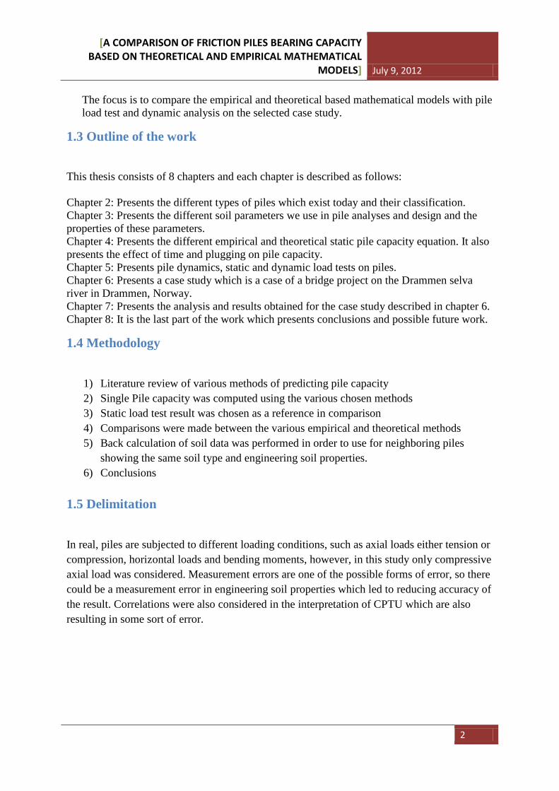
2.1.1 Friction piles If the piles do not reach a hard stratum, their load carrying capacity is derived partly from end bearing and partly from the skin friction; these piles are called friction piles.
Figure 2.1 Friction pile [2]
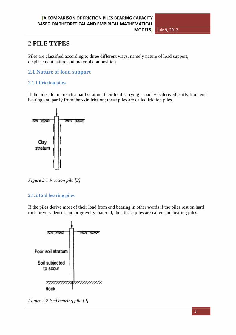
2.1.2 End bearing piles If the piles derive most of their load from end bearing in other words if the piles rest on hard rock or very dense sand or gravelly material, then these piles are called end bearing piles.
Figure 2.2 End bearing pile [2]
[A COMPARISON OF FRICTION PILES BEARING CAPACITY BASED ON THEORETICAL AND EMPIRICAL MATHEMATICAL
MODELS] July 9, 2012
4
2.2 Displacement nature
2.2.1 Displacement piles Displacement piles are those piles, which displace the soil radially and vertically during driving. Example: Closed pipe piles. 2.2.2 Partial-displacement piles Partial-displacement piles are those piles showing behavior intermediate between full-displacement and non-displacement piles. They displace smaller volume of soil. Example: Open end pipe pile, H-piles.
2.2.3 Non-displacement piles Non-displacement piles are those piles which are casted after boring. They are also called replacement piles. Example: bored piles (Example: Franki piles)
2.3 Material composition
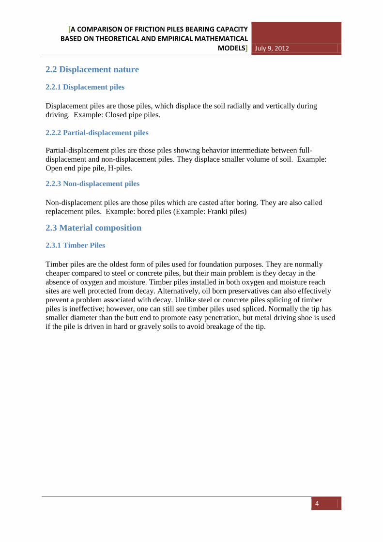
2.3.1 Timber Piles Timber piles are the oldest form of piles used for foundation purposes. They are normally cheaper compared to steel or concrete piles, but their main problem is they decay in the absence of oxygen and moisture. Timber piles installed in both oxygen and moisture reach sites are well protected from decay. Alternatively, oil born preservatives can also effectively prevent a problem associated with decay. Unlike steel or concrete piles splicing of timber piles is ineffective; however, one can still see timber piles used spliced. Normally the tip has smaller diameter than the butt end to promote easy penetration, but metal driving shoe is used if the pile is driven in hard or gravely soils to avoid breakage of the tip.
[A COMPARISON OF FRICTION PILES BEARING CAPACITY BASED ON THEORETICAL AND EMPIRICAL MATHEMATICAL
MODELS] July 9, 2012
5
Figure 2.3 Timber piles used as foundation material in the city of Trondheim (after Ermias)
2.3.2 Concrete piles Precast concrete piles: also known as ”prefabricated piles” are produced in a casting yard in a location away from the building site or close to the building site if sufficient space is available and great demand of more piles and transported to the construction site. According to Bowles (1996) precast piles using ordinary reinforcement are designed to resist bending stresses during pick up and transport to the site and bending moments from lateral loads and to provide sufficient resistance to vertical loads and any tension forces developed during driving.
[A COMPARISON OF FRICTION PILES BEARING CAPACITY BASED ON THEORETICAL AND EMPIRICAL MATHEMATICAL
MODELS] July 9, 2012
6
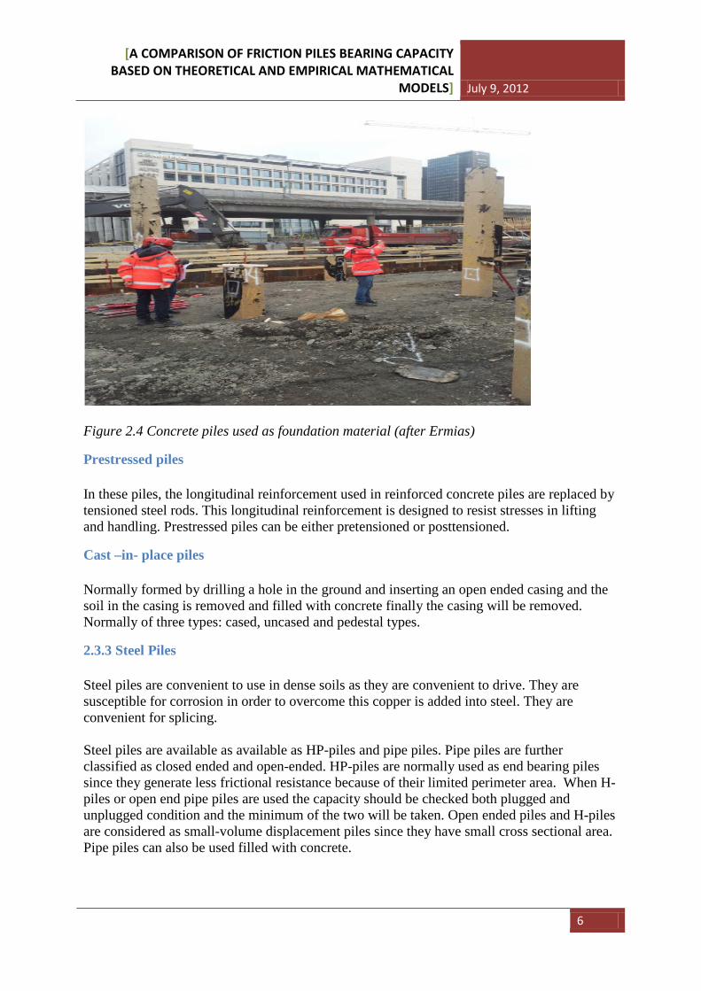
Figure 2.4 Concrete piles used as foundation material (after Ermias)
Prestressed piles In these piles, the longitudinal reinforcement used in reinforced concrete piles are replaced by tensioned steel rods. This longitudinal reinforcement is designed to resist stresses in lifting and handling. Prestressed piles can be either pretensioned or posttensioned.
Cast –in- place piles Normally formed by drilling a hole in the ground and inserting an open ended casing and the soil in the casing is removed and filled with concrete finally the casing will be removed. Normally of three types: cased, uncased and pedestal types.
2.3.3 Steel Piles Steel piles are convenient to use in dense soils as they are convenient to drive. They are susceptible for corrosion in order to overcome this copper is added into steel. They are convenient for splicing. Steel piles are available as available as HP-piles and pipe piles. Pipe piles are further classified as closed ended and open-ended. HP-piles are normally used as end bearing piles since they generate less frictional resistance because of their limited perimeter area. When H-piles or open end pipe piles are used the capacity should be checked both plugged and unplugged condition and the minimum of the two will be taken. Open ended piles and H-piles are considered as small-volume displacement piles since they have small cross sectional area. Pipe piles can also be used filled with concrete.
[A COMPARISON OF FRICTION PILES BEARING CAPACITY BASED ON THEORETICAL AND EMPIRICAL MATHEMATICAL
MODELS] July 9, 2012
7
3 SOIL PARAMETERS FOR PILE ANALYSIS AND DESIGN
Soil investigations generally proceed through following four phases [15]:
1) Preliminary Soil Investigations 2) Detailed Soil Investigations 3) Construction Verification 4) Post Construction Monitoring
3.1 Scope, objectives and extent of the soil investigation
The objectives of foundations soil investigation are to determine the extent, thickness, and properties of the soils and rocks and the ground water levels at a site [15]. It is carried out in a way soil stratigraphy is described in detail with sufficient test pits.
The extent of the investigation depends on the following factors:
Character of the soil Available information from previous experience The degree of variation of the soils around the site The importance of the structure
3.2 Various soil investigation and testing methods
One way of performing soil investigation is by soil boring this can be accomplished by retrieving sample for laboratory testing which in turn result in possible conclusion of the stratigraphy and soil parameters.
3.2.1 Boring techniques
Here some of the different boring techniques used in different part of the world
- Auger boring - Wash boring - Rotary drilling - Percussion drilling
3.2.2 Soil sampling and laboratory testing In Scandinavia, the piston sampler with diameter 54mm is widely used to retrieve a sample for a possible laboratory testing program. Depending on the type of test we accomplish we retrieve either a disturbed or undisturbed sample.
[A COMPARISON OF FRICTION PILES BEARING CAPACITY BASED ON THEORETICAL AND EMPIRICAL MATHEMATICAL
MODELS] July 9, 2012
8
Laboratory testing is carried out to classify the soils and to provide soil parameter for design. The following are some of the properties of soils determined in the laboratory.
Unit weight (γ )
Basically calculated as dividing the total weight of soil by volume of soil.
w s
v s
w wwv v v
γ += =
+ (3-1)
Relative density ( rD )
It is an important parameter defining cohesionless soils. Basically defined as:
max
max min
ne eDre e
−=
− Or, (3-2)
min max
max min
( )( )nr
n
D γ γ γγ γ γ
−=
− (3-3)
Water content ( w )
The natural water content ( nw ) is determined from disturbed soil sample. The sample is weighed first and then oven dried and weighed again from this procedure the water content can be determined.
Atterberg limits
The liquid limit and plastic limit is routinely determined for cohesive soils and using these values, plasticity index is determined. p L pI w w= − (3-4)
Overconsolidation
A soil is called normally consolidated if the current stress level is the largest in the history of the soil. While the soil is over consolidated if the soil is exposed to a stress larger than the present stress in its history.
''c
o
pOCRp
= (3-5)
'cp = preconsolidation pressure 'op = current overburden pressure A normally consolidated soil has OCR =1 and overconsolidated soil has OCR >1.
[A COMPARISON OF FRICTION PILES BEARING CAPACITY BASED ON THEORETICAL AND EMPIRICAL MATHEMATICAL
MODELS] July 9, 2012
9
3.2.3 Field testing The following field testing methods are commonly used in various parts of the world
Standard penetration test (SPT)
The main goal of this test is to determine SPT N value, and the SPT N value is empirically related to many engineering properties of soils. In literatures, one can find different engineering properties of soils correlated with SPT N value.
The test is performed by attaching a split spoon sampler to the bottom of the core barrel and lowered into the desired position at the bottom of the borehole, and then the sampler is driven into the ground by a drop hammer weighing 68Kg falling from a height of 76cm. The number of blow required to drive the sampler three successive 150mm increments is registered. The first increment (0-150mm) is not included in the N value as it is believed to be disturbed by the drilling. The N value is the number of blows required to assist the last two increments (150mm-450mm). Finally, the N value should be corrected to the standard energy.
Cone penetration test (CPT)
The CPT is one of the in-situ tests commonly used in Norway. It was first discovered in the Netherlands. It is available as Dutch cone, electric cone, electric piezo, electric piezo/friction and seismic cone. Continuous measurement is taken for both the soil resistance and the sleeve friction by putting the cone at the end of serious rods. Penetration rate is 2cm/sec. Nearly 95% of offshore investigation is carried out using the CPT.
The following parameters can be determined from the CPTU:
• Undrained shear strength, u
s • The soil unit weight • Pre-consolidation pressure, cp • Friction angle, φ • Deformation modulus, M , G • Coefficient of consolidation, cc
Corrected cone resistance and sleeve friction can be obtained by correcting the tip resistance and sleeve friction for pore pressure acting on the geometry. 2(1 )t cq q a u= + − (3-6) Where
[A COMPARISON OF FRICTION PILES BEARING CAPACITY BASED ON THEORETICAL AND EMPIRICAL MATHEMATICAL
MODELS] July 9, 2012
10
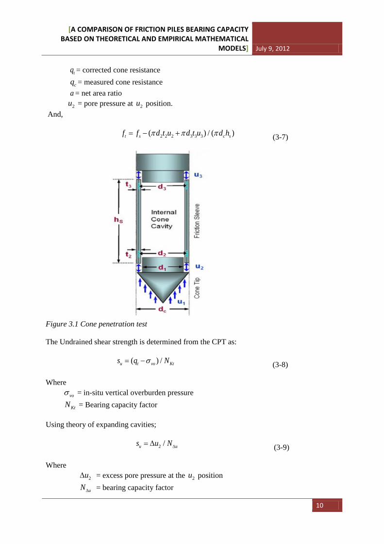
tq = corrected cone resistance cq = measured cone resistance a = net area ratio 2u = pore pressure at 2u position. And, 2 2 2 3 3 3( ) / ( )t s c sf f d t u d t u d hπ π π= − + (3-7)
Figure 3.1 Cone penetration test The Undrained shear strength is determined from the CPT as: ( ) /u t vo Kts q Nσ= − (3-8) Where voσ = in-situ vertical overburden pressure KtN = Bearing capacity factor Using theory of expanding cavities; 2 /u us u N∆= ∆ (3-9)
Where 2u∆ = excess pore pressure at the 2u position uN∆ = bearing capacity factor
[A COMPARISON OF FRICTION PILES BEARING CAPACITY BASED ON THEORETICAL AND EMPIRICAL MATHEMATICAL
MODELS] July 9, 2012
11
Vane shear test
The vane shear test is commonly used field test for the interpretation of undrained shear strength and sensitivity of cohesive soils. The blade has a height-to-diameter ratio of 2. The test is performed by inserting the vane into the soil and applying the torque for about 5 to 10 minutes and the required torque to cause shearing is measured and the undrained strength is calculated using equation 𝑆𝑢𝑣 = 6𝑇
7𝜋𝐷3 (3-10)
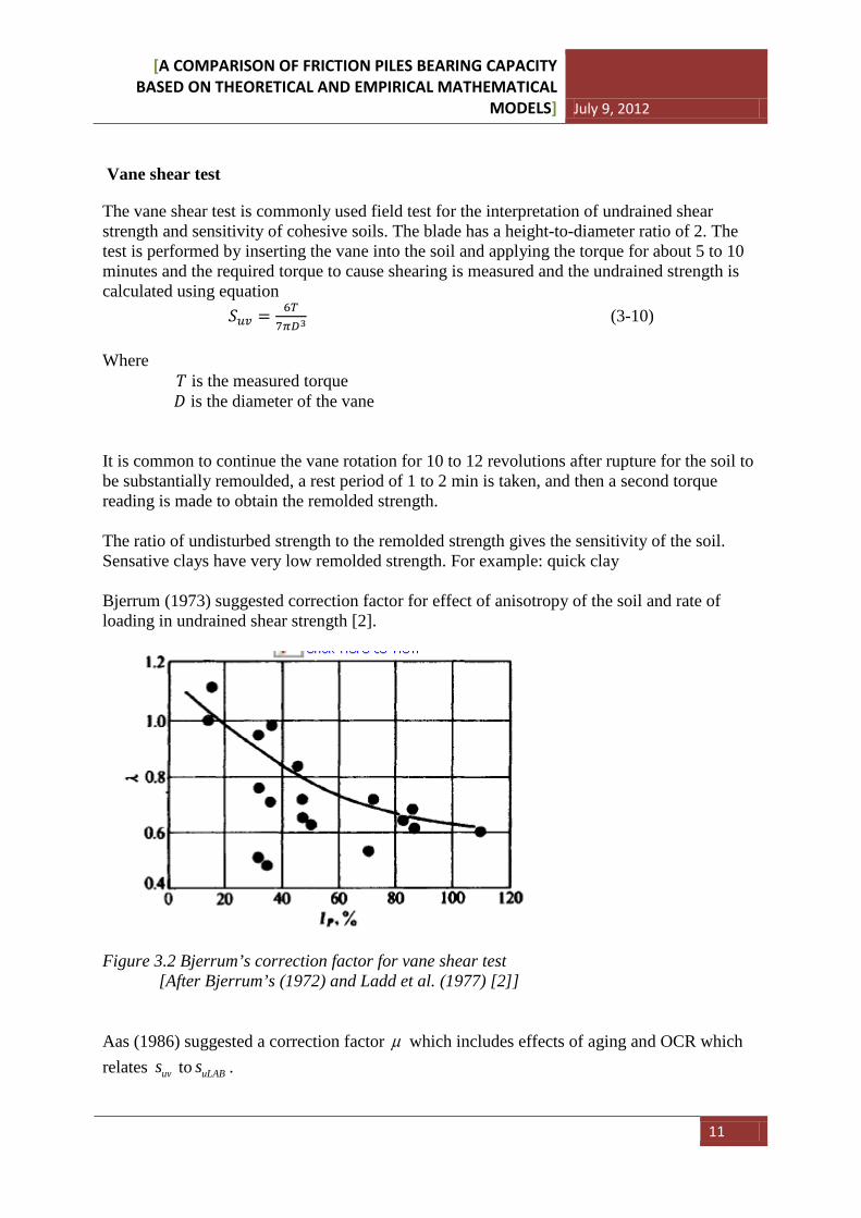
Where 𝑇 is the measured torque 𝐷 is the diameter of the vane It is common to continue the vane rotation for 10 to 12 revolutions after rupture for the soil to be substantially remoulded, a rest period of 1 to 2 min is taken, and then a second torque reading is made to obtain the remolded strength. The ratio of undisturbed strength to the remolded strength gives the sensitivity of the soil. Sensative clays have very low remolded strength. For example: quick clay Bjerrum (1973) suggested correction factor for effect of anisotropy of the soil and rate of loading in undrained shear strength [2].
Figure 3.2 Bjerrum’s correction factor for vane shear test [After Bjerrum’s (1972) and Ladd et al. (1977) [2]] Aas (1986) suggested a correction factor µ which includes effects of aging and OCR which relates uvs to uLABs .
[A COMPARISON OF FRICTION PILES BEARING CAPACITY BASED ON THEORETICAL AND EMPIRICAL MATHEMATICAL
MODELS] July 9, 2012
12
Where
( )
3uA uD up
uLAB
s s ss
+ +=
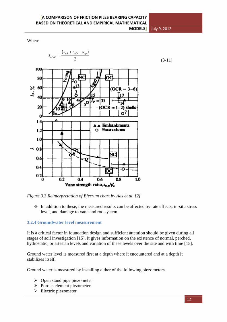
(3-11)
Figure 3.3 Reinterpretation of Bjerrum chart by Aas et al. [2] In addition to these, the measured results can be affected by rate effects, in-situ stress
level, and damage to vane and rod system. 3.2.4 Groundwater level measurement It is a critical factor in foundation design and sufficient attention should be given during all stages of soil investigation [15]. It gives information on the existence of normal, perched, hydrostatic, or artesian levels and variation of these levels over the site and with time [15]. Ground water level is measured first at a depth where it encountered and at a depth it stabilizes itself. Ground water is measured by installing either of the following piezometers. Open stand pipe piezometer Porous element piezometer Electric piezometer
[A COMPARISON OF FRICTION PILES BEARING CAPACITY BASED ON THEORETICAL AND EMPIRICAL MATHEMATICAL
MODELS] July 9, 2012
13
Pneumatic piezometer
3.3 Design parameters
3.3.1 Strength parameters The strength parameters needed are cohesion ( c ) and angle of internal friction (φ ). They are determined from laboratory tests on undisturbed sample using the triaxial apparatus. Basically there are three types of triaxial test: 1) Unconsolidated undrained (UU) tests. 2) Consolidated undrained (CU) tests. 3) Consolidated drained (CD) tests. We can also determine the c and φ using direct shear or direct simple shear apparatus. Undrained shear strength ( us )
Can be determined from unconfined compressive tests, triaxial test, fall cone test, vane shear test or CPT.
For normally consolidated soils, us can be estimated as according to Skempton and Henkel (1953) [2].
' (0.1 0.004 )u vs PIσ= + (3-12) According to Bjerrum and Simons (1960)
𝑠𝑢𝑝0′
= 0.45(𝐼𝑃)0.5 𝐼𝑃 > 0.5 (3-13)
𝑠𝑢𝑝0′
= 0.18(𝐼𝐿)0.5 𝐼𝐿 > 0.5 (3-14)
Sensativity
Sensativity is the ratio of undisturbed strength to the remolded strength. ts = Undisturbed strength Remolded stregth Thixotropy
Thixotropy is the regain of strength from remolded state with time. Driven piles in soft clay deposite often have very little load carrying capacity until a combination of aging/cementation (thixotropy) and dissipation of excess pore pressure (consolidation) occurs [2].
[A COMPARISON OF FRICTION PILES BEARING CAPACITY BASED ON THEORETICAL AND EMPIRICAL MATHEMATICAL
MODELS] July 9, 2012
14
3.3.2 Soil pile adhesion It is quite difficult to determine. A back calculation of static load test on a prototype foundation can only give a reliable result. It is affected by factors such as consistency of the soil, method of installation of the pile, material which the pile is made from, and the time after installation.
3.3.3 Elastic soil parameters
The most common elastic soil parameter in the design of pile is the modulus of elasticity, 𝐸𝑠 [14].
[A COMPARISON OF FRICTION PILES BEARING CAPACITY BASED ON THEORETICAL AND EMPIRICAL MATHEMATICAL
MODELS] July 9, 2012
15
4 STATIC PILE CAPACITY
Generally, we determine the capacity of a pile in two alternative ways i.e.
1) Testing e.g. static load test and dynamic load test 2) Calculation e.g. static design equations based on laboratory and field investigations
and pile driving formula
Sufficient emphasis should be given to the accuracy in the estimation of pile capacity, this will lead us to not only to safer structure but also to economic savings. It should be noted that the term capacity in this thesis refers to capacity of the bearing soil and it is not the structural strength of the pile itself.
The ultimate axial load carrying capacity of piles should be determined by the equation:
u p s p p s sQ Q Q q A f A= + = + (4-1)
And design load capacity, in other words allowable bearing capacity is given as
ua
QQFS
= (4-2)
Where 𝑒𝑒𝐴
=𝜋𝑟2𝐴
=𝜋𝑟2
𝑄𝑢 = Ultimate pile capacity
𝑄𝑎 = Allowable pile capacity
𝑞𝑝 = Unit pile tip resistance
𝑓𝑠 = Unit skin friction capacity
𝐴𝑝 = The pile tip area
𝐴𝑠 = The pile side area
𝐹𝑆 = Factor of safety
The following Parameters affect the capacity of piles
1) Pile characteristics
- Geometry ( diameter, wall thickness, penetration ratio)
[A COMPARISON OF FRICTION PILES BEARING CAPACITY BASED ON THEORETICAL AND EMPIRICAL MATHEMATICAL
MODELS] July 9, 2012
16
- Tip detail ( weather it is open-ended or closed-ended; driving shoe) - Material, roughness
2) Loading condition
- Weather subjected to tension or compression load - Weather subjected to static or cyclic load - Weather vertical load alone or in combination with horizontal load or moments - Time between driving and loading
3) Installation
- Rate of penetration - Continuity of penetration - Installation methods, i.e. driving, jacking or vibration - Mode of penetration, i.e. weather it is plugged or not
4) Soil characteristics
- Soil stratigraphy - In situ stress state - Stress history in other words over consolidation ratio (𝑂𝐶𝑅) - Undrained shear strength - Plasticity Index ( 𝐼𝑃) - Sensitivity - Relative density - Cone resistance value, 𝑞𝑐 - Pile soil interface friction angle,
4.1 Empirical Methods
4.1.1 Method based on Cone penetration test (CPT)
Since invented, the cone penetration test has been used to estimate pile capacity. Over the years, a number of other empirical methods have been developed to estimate the capacities of pile, for instance the schmertmann method (schmertmann 1978), the Dutch method (de Ruiter and Beringen 1979) and some more others too.
[A COMPARISON OF FRICTION PILES BEARING CAPACITY BASED ON THEORETICAL AND EMPIRICAL MATHEMATICAL
MODELS] July 9, 2012
17
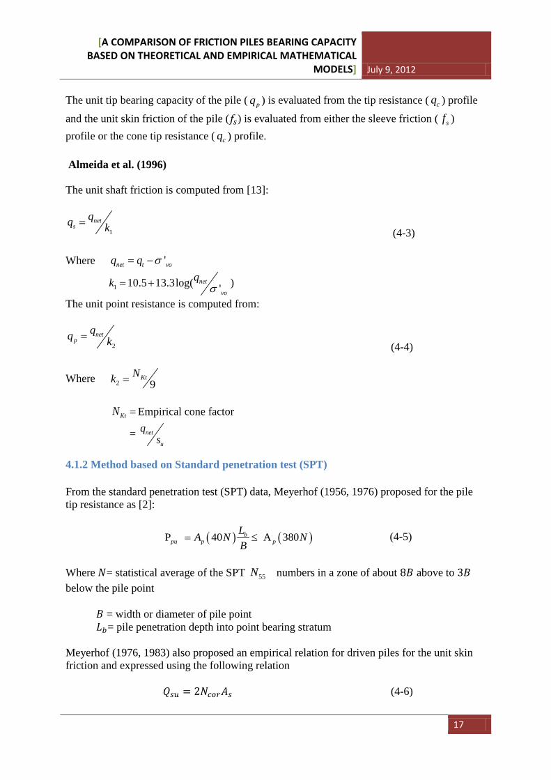
The unit tip bearing capacity of the pile ( pq ) is evaluated from the tip resistance ( cq ) profile
and the unit skin friction of the pile (𝑓𝑠) is evaluated from either the sleeve friction ( sf ) profile or the cone tip resistance ( cq ) profile. Almeida et al. (1996) The unit shaft friction is computed from [13]:
1
nets
qq k= (4-3)
Where 'net t voq q σ= −
1 10.5 13.3log( 'net
vo
qk σ= + )
The unit point resistance is computed from:
2
netp
qq k= (4-4)
Where 2 9KtNk =
KtN =Empirical cone factor
= net
u
qs
4.1.2 Method based on Standard penetration test (SPT) From the standard penetration test (SPT) data, Meyerhof (1956, 1976) proposed for the pile tip resistance as [2]:
( ) ( ) P 40 A 380bpu p p
LA N NB
= ≤ (4-5)
Where 𝑁= statistical average of the SPT 55N numbers in a zone of about 8𝐵 above to 3𝐵 below the pile point 𝐵 = width or diameter of pile point 𝐿𝑏= pile penetration depth into point bearing stratum Meyerhof (1976, 1983) also proposed an empirical relation for driven piles for the unit skin friction and expressed using the following relation 𝑄𝑠𝑢 = 2𝑁𝑐𝑜𝑟𝐴𝑠 (4-6)
[A COMPARISON OF FRICTION PILES BEARING CAPACITY BASED ON THEORETICAL AND EMPIRICAL MATHEMATICAL
MODELS] July 9, 2012
18
Where 𝑄𝑠𝑢 = Ultimate skin friction in 𝐾𝑃𝑎 𝑁𝑐𝑜𝑟 = corrected SPT N value 𝐴𝑠 = Skin friction contact area
4.1.3 Axial pile capacity in clay using various pile design practices
Pile skin capacity
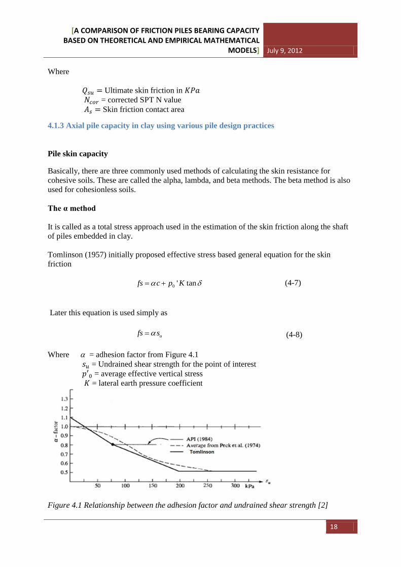
Basically, there are three commonly used methods of calculating the skin resistance for cohesive soils. These are called the alpha, lambda, and beta methods. The beta method is also used for cohesionless soils. The α method It is called as a total stress approach used in the estimation of the skin friction along the shaft of piles embedded in clay. Tomlinson (1957) initially proposed effective stress based general equation for the skin friction 0 ' tanfs c p Kα δ= + (4-7) Later this equation is used simply as ufs sα= (4-8) Where α = adhesion factor from Figure 4.1 𝑠𝑢 = Undrained shear strength for the point of interest 𝑝′0 = average effective vertical stress 𝐾 = lateral earth pressure coefficient
Figure 4.1 Relationship between the adhesion factor and undrained shear strength [2]
[A COMPARISON OF FRICTION PILES BEARING CAPACITY BASED ON THEORETICAL AND EMPIRICAL MATHEMATICAL
MODELS] July 9, 2012
19
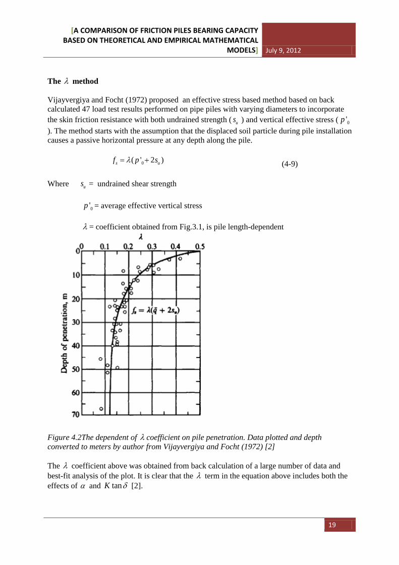
The λ method Vijayvergiya and Focht (1972) proposed an effective stress based method based on back calculated 47 load test results performed on pipe piles with varying diameters to incorporate the skin friction resistance with both undrained strength ( us ) and vertical effective stress ( 0'p). The method starts with the assumption that the displaced soil particle during pile installation causes a passive horizontal pressure at any depth along the pile. 0( ' 2 )s uf p sλ= + (4-9) Where us = undrained shear strength 0'p = average effective vertical stress λ = coefficient obtained from Fig.3.1, is pile length-dependent
Figure 4.2The dependent of λ coefficient on pile penetration. Data plotted and depth converted to meters by author from Vijayvergiya and Focht (1972) [2] The λ coefficient above was obtained from back calculation of a large number of data and best-fit analysis of the plot. It is clear that the λ term in the equation above includes both the effects of α and tanK δ [2].
[A COMPARISON OF FRICTION PILES BEARING CAPACITY BASED ON THEORETICAL AND EMPIRICAL MATHEMATICAL
MODELS] July 9, 2012
20
The β method Surprisingly, Burland (1973) developed an effective stress based method from load tests on bored piles, but has gained wide spread acceptance in designing driven piles. The equation looks like of the form: 0' tansf Kp δ= (4-10)
Taking tanKβ δ= , the equation for the skin resistance can be rewritten as
sf qβ−
= (4-11)
0'p = average effective vertical stress
This method is recommended only for cohesionless soils. Meyerhof (1976) extended Burland’s approach for overconsolidated clay. 𝛽𝑂𝐶 = (1 ± 0.5)𝛽𝑁𝐶√𝑂𝐶𝑅
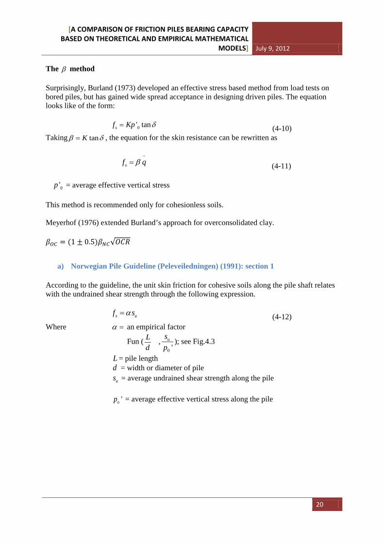
a) Norwegian Pile Guideline (Peleveiledningen) (1991): section 1 According to the guideline, the unit skin friction for cohesive soils along the pile shaft relates with the undrained shear strength through the following expression. s uf sα= (4-12)
Where α = an empirical factor
Fun ( Ld
,0 'us
p); see Fig.4.3
L = pile length d = width or diameter of pile us = average undrained shear strength along the pile 'op = average effective vertical stress along the pile
[A COMPARISON OF FRICTION PILES BEARING CAPACITY BASED ON THEORETICAL AND EMPIRICAL MATHEMATICAL
MODELS] July 9, 2012
21
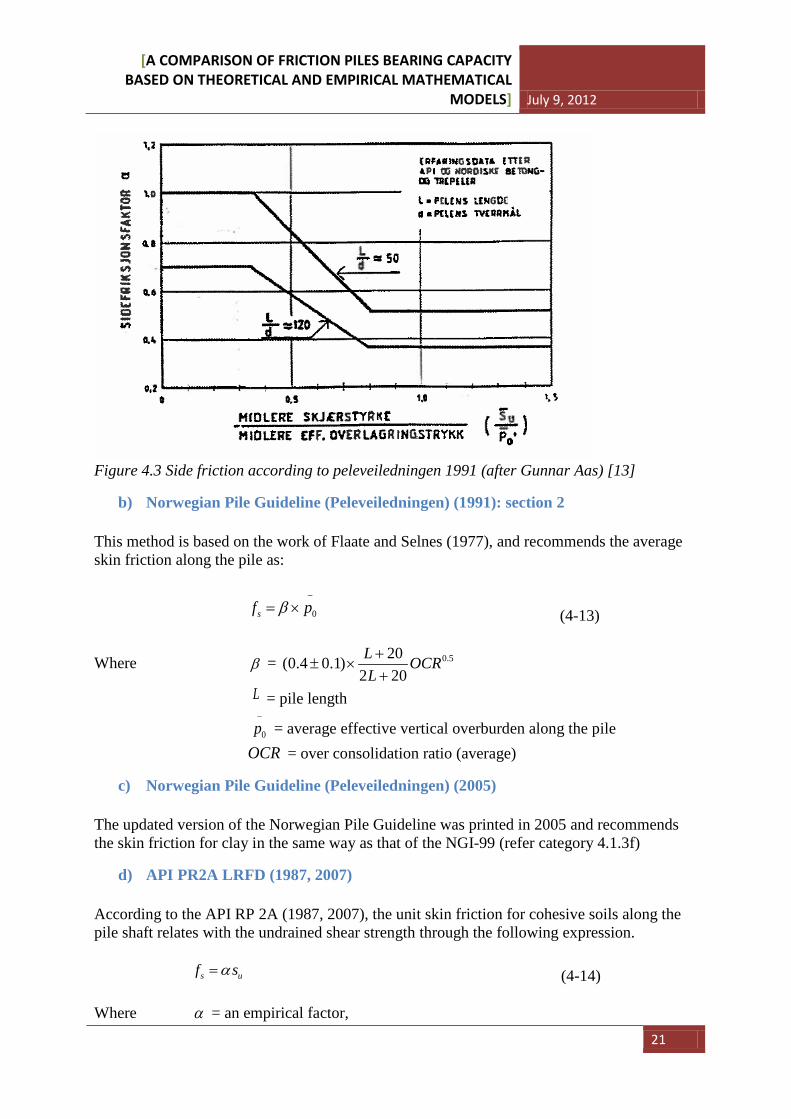
Figure 4.3 Side friction according to peleveiledningen 1991 (after Gunnar Aas) [13]
b) Norwegian Pile Guideline (Peleveiledningen) (1991): section 2 This method is based on the work of Flaate and Selnes (1977), and recommends the average skin friction along the pile as:
0sf pβ−
= × (4-13)
Where β = 0.520(0.4 0.1)2 20L OCRL+
± ×+
= pile length
0p−
= average effective vertical overburden along the pile OCR = over consolidation ratio (average)
c) Norwegian Pile Guideline (Peleveiledningen) (2005) The updated version of the Norwegian Pile Guideline was printed in 2005 and recommends the skin friction for clay in the same way as that of the NGI-99 (refer category 4.1.3f)
d) API PR2A LRFD (1987, 2007) According to the API RP 2A (1987, 2007), the unit skin friction for cohesive soils along the pile shaft relates with the undrained shear strength through the following expression. s uf sα= (4-14) Where α = an empirical factor,
L
[A COMPARISON OF FRICTION PILES BEARING CAPACITY BASED ON THEORETICAL AND EMPIRICAL MATHEMATICAL
MODELS] July 9, 2012
22
us = average undrained shear strength along the pile The factor,α , can be computed by the equations: 0.50.5α ψ −= 1.0ψ ≤ 0.250.5α ψ −= 0ψ > With the constrain that, 1α ≤ , ψ =
0'c
p for the point in question.
0'p = effective vertical stress at the point in question
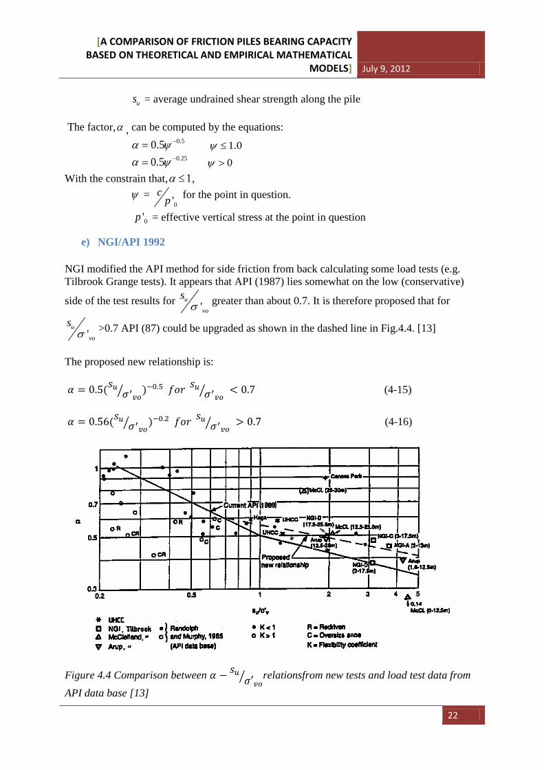
e) NGI/API 1992 NGI modified the API method for side friction from back calculating some load tests (e.g. Tilbrook Grange tests). It appears that API (1987) lies somewhat on the low (conservative)
side of the test results for 'u
vo
sσ greater than about 0.7. It is therefore proposed that for
'u
vo
sσ >0.7 API (87) could be upgraded as shown in the dashed line in Fig.4.4. [13]
The proposed new relationship is: 𝛼 = 0.5(𝑠𝑢 𝜎′𝑣𝑜� )−0.5 𝑓𝑜𝑟 𝑠𝑢 𝜎′𝑣𝑜 � < 0.7 (4-15) 𝛼 = 0.56(𝑠𝑢 𝜎′𝑣𝑜� )−0.2 𝑓𝑜𝑟 𝑠𝑢 𝜎′𝑣𝑜 � > 0.7 (4-16)
Figure 4.4 Comparison between 𝛼 − 𝑠𝑢
𝜎′𝑣𝑜� relationsfrom new tests and load test data from API data base [13]
[A COMPARISON OF FRICTION PILES BEARING CAPACITY BASED ON THEORETICAL AND EMPIRICAL MATHEMATICAL
MODELS] July 9, 2012
23
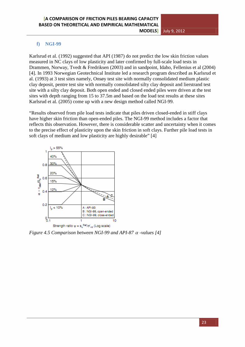
f) NGI-99 Karlsrud et al. (1992) suggested that API (1987) do not predict the low skin friction values measured in NC clays of low plasticity and later confirmed by full-scale load tests in Drammen, Norway, Tvedt & Fredriksen (2003) and in sandpoint, Idaho, Fellenius et al (2004) [4]. In 1993 Norwegian Geotechnical Institute led a research program described as Karlsrud et al. (1993) at 3 test sites namely, Onsøy test site with normally consolidated medium plastic clay deposit, pentre test site with normally consolidated silty clay deposit and lierstrand test site with a silty clay deposit. Both open ended and closed ended piles were driven at the test sites with depth ranging from 15 to 37.5m and based on the load test results at these sites Karlsrud et al. (2005) come up with a new design method called NGI-99. “Results observed from pile load tests indicate that piles driven closed-ended in stiff clays have higher skin friction than open-ended piles. The NGI-99 method includes a factor that reflects this observation. However, there is considerable scatter and uncertainty when it comes to the precise effect of plasticity upon the skin friction in soft clays. Further pile load tests in soft clays of medium and low plasticity are highly desirable” [4]
Figure 4.5 Comparison between NGI-99 and API-87 α -values [4]
[A COMPARISON OF FRICTION PILES BEARING CAPACITY BASED ON THEORETICAL AND EMPIRICAL MATHEMATICAL
MODELS] July 9, 2012
24
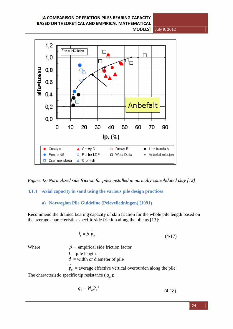
Figure 4.6 Normalized side friction for piles installed in normally consolidated clay [12] 4.1.4 Axial capacity in sand using the various pile design practices
a) Norwegian Pile Guideline (Peleveiledningen) (1991)
Recommend the drained bearing capacity of skin friction for the whole pile length based on the average characteristics specific side friction along the pile as [13]:
s of pβ−
= (4-17)
Where β = empirical side friction factor L = pile length d = width or diameter of pile
0p−
= average effective vertical overburden along the pile. The characteristic specific tip resistance ( pq ):
'p q pq N P= (4-18)
[A COMPARISON OF FRICTION PILES BEARING CAPACITY BASED ON THEORETICAL AND EMPIRICAL MATHEMATICAL
MODELS] July 9, 2012
25
Where qN = bearing capacity factor 'pP = effective vertical overburden pressure at pile tip.
a) b)
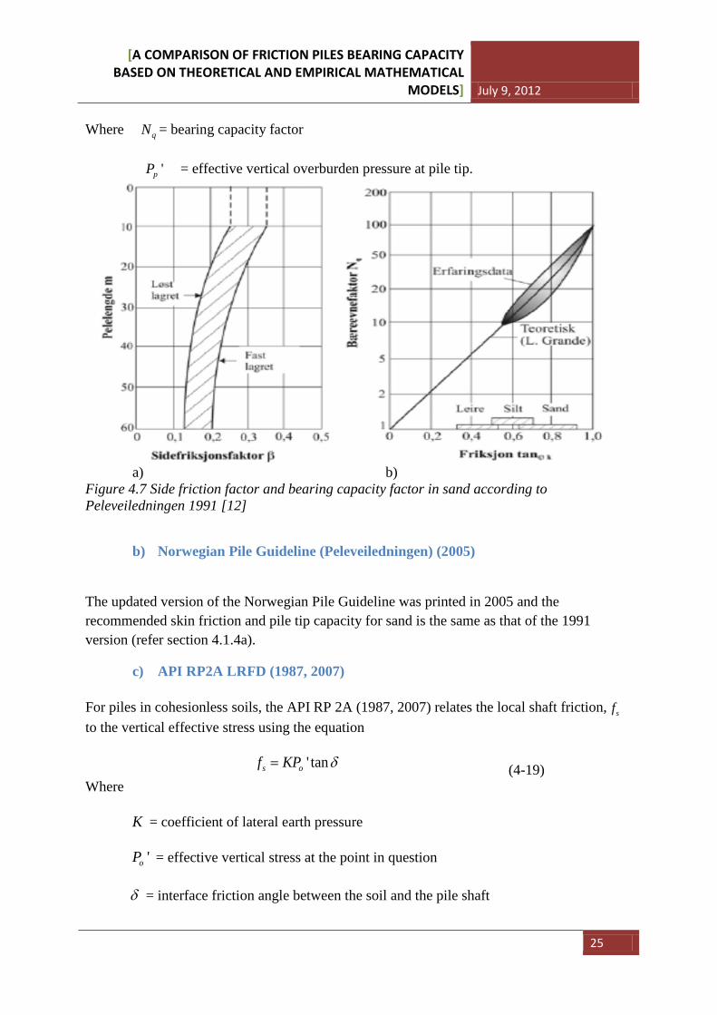
Figure 4.7 Side friction factor and bearing capacity factor in sand according to Peleveiledningen 1991 [12]
b) Norwegian Pile Guideline (Peleveiledningen) (2005)
The updated version of the Norwegian Pile Guideline was printed in 2005 and the recommended skin friction and pile tip capacity for sand is the same as that of the 1991 version (refer section 4.1.4a).
c) API RP2A LRFD (1987, 2007) For piles in cohesionless soils, the API RP 2A (1987, 2007) relates the local shaft friction, sf to the vertical effective stress using the equation ' tans of KP δ= (4-19)
Where K = coefficient of lateral earth pressure
'oP = effective vertical stress at the point in question δ = interface friction angle between the soil and the pile shaft
[A COMPARISON OF FRICTION PILES BEARING CAPACITY BASED ON THEORETICAL AND EMPIRICAL MATHEMATICAL
MODELS] July 9, 2012
26
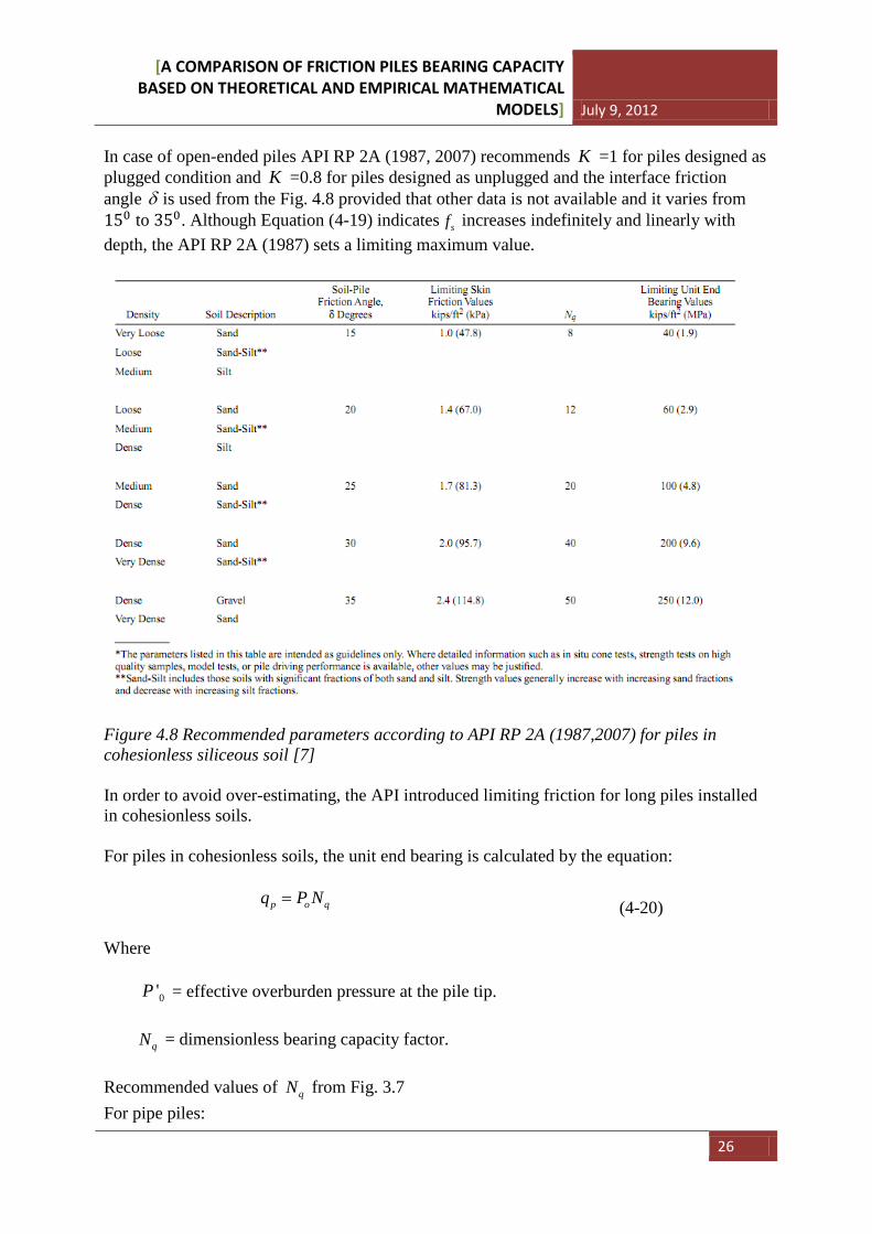
In case of open-ended piles API RP 2A (1987, 2007) recommends K =1 for piles designed as plugged condition and K =0.8 for piles designed as unplugged and the interface friction angle δ is used from the Fig. 4.8 provided that other data is not available and it varies from 150 to 350. Although Equation (4-19) indicates sf increases indefinitely and linearly with depth, the API RP 2A (1987) sets a limiting maximum value.
Figure 4.8 Recommended parameters according to API RP 2A (1987,2007) for piles in cohesionless siliceous soil [7] In order to avoid over-estimating, the API introduced limiting friction for long piles installed in cohesionless soils. For piles in cohesionless soils, the unit end bearing is calculated by the equation: p o qq P N= (4-20)
Where 0'P = effective overburden pressure at the pile tip.
qN = dimensionless bearing capacity factor. Recommended values of qN from Fig. 3.7 For pipe piles:
[A COMPARISON OF FRICTION PILES BEARING CAPACITY BASED ON THEORETICAL AND EMPIRICAL MATHEMATICAL
MODELS] July 9, 2012
27
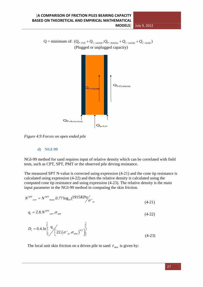
Q = minimum of: ( ; )P Full f outside P Annulus f outside f insideQ Q Q Q Q− − − − −+ + + (Plugged or unplugged capacity)
Figure 4.9 Forces on open ended pile
d) NGI-99 NGI-99 method for sand requires input of relative density which can be correlated with field tests, such as CPT, SPT, PMT or the observed pile driving resistance. The measured SPT N-value is corrected using expression (4-21) and the cone tip resistance is calculated using expression (4-22) and then the relative density is calculated using the computed cone tip resistance and using expression (4-23). The relative density is the main input parameter in the NGI-99 method in computing the skin friction.
101915.0.77 log ( '
SPT SPTcorr meas
vo
KPaN N σ= (4-21)
2.8. .SPT
c corr atmq N σ= (4-22)
( )0.50.4.ln22. ' .
cr
vo atm
qDσ σ
= (4-23)
The local unit skin friction on a driven pile in sand skinτ is given by:
[A COMPARISON OF FRICTION PILES BEARING CAPACITY BASED ON THEORETICAL AND EMPIRICAL MATHEMATICAL
MODELS] July 9, 2012
28
sin ( ) . . . . . .tip atm Dr sig tip load mat
zz z F F F F Fτ σ= (4-24)
( ) 0.1. 'skin vozτ σ>
z = depth below the ground surface
tipz = pile tip depth
atmσ = atmospheric reference pressure = 100KPa
1.72.1.( 0.1)Dr rF D= −
0.25'( )vosig
atmF σ
σ=
tipF = 1.0 for a pile driven open-ended, 1.6 for a close-ended pile
loadF = 1.0 for tension, 1.3 for compression
matF = 1.0 for steel and 1.2 for concrete The point resistance acting against a pile driven close-ended is given by:
( )20.8.1
ctip
qDr
σ =+
The plugged tip resistance of an open-ended pile is calculated as:
( )20.7.1 3.
ctip
qDr
σ =+
4.2 Theoretical method The theoretical methods presented in this study comply with the Norwegian University of Science and Technology (NTNU) way of teaching.
4.2.1 Short term capacity
a) Shaft friction Based on the earth pressure approach the shaft friction is estimated from
us c
sr rFS
τ τ= = (4-25)
Where:
[A COMPARISON OF FRICTION PILES BEARING CAPACITY BASED ON THEORETICAL AND EMPIRICAL MATHEMATICAL
MODELS] July 9, 2012
29
r is a combination of roughness ratio and remolding caused by the pile driving following reconsolidation.
usFS
= mobilized undrained shear strength in depth z.
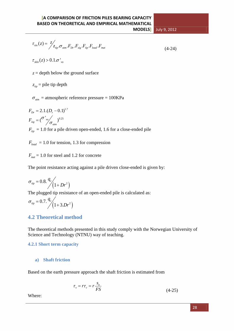
Figure 4.10 Side friction derivation using earth pressure concept (after Lars Janbu)
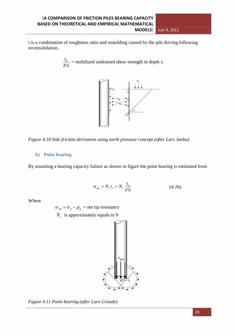
b) Point bearing By assuming a bearing capacity failure as shown in figure the point bearing is estimated from
upn c c c
sN NFS
σ τ= = (4-26)
Where pn p ppσ σ= − = net tip resistance
cN is approximately equals to 9
Figure 4.11 Point bearing (after Lars Grande)
[A COMPARISON OF FRICTION PILES BEARING CAPACITY BASED ON THEORETICAL AND EMPIRICAL MATHEMATICAL
MODELS] July 9, 2012
30
4.2.2 Long term capacity
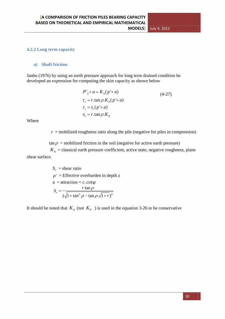
a) Shaft friction Janbu (1976) by using an earth pressure approach for long term drained condition he developed an expression for computing the skin capacity as shown below ' ( ' )a AP a K p a+ = + (4-27)
. tan . ( ' )s Ar K p aτ ρ= + ( ' )s vs p aτ = + . tan .v As r Kρ= Where r = mobilized roughness ratio along the pile (negative for piles in compression) tan ρ = mobilized friction in the soil (negative for active earth pressure) AK = classical earth pressure coefficient, active state, negative roughness, plane shear surface. vS = shear ratio
'p = Effective overburden in depth z a = attraction = 𝑐. 𝑐𝑜𝑡𝜑
2 2
tan
( 1 tan tan . 1 )v
rSr
ρ
ρ ρ=
+ − + It should be noted that AK (not PK ) is used in the equation 3-26 to be conservative
[A COMPARISON OF FRICTION PILES BEARING CAPACITY BASED ON THEORETICAL AND EMPIRICAL MATHEMATICAL
MODELS] July 9, 2012
31
Figure 4.12 vS vs. tan ρ chart for compressive pile (after Janbu)
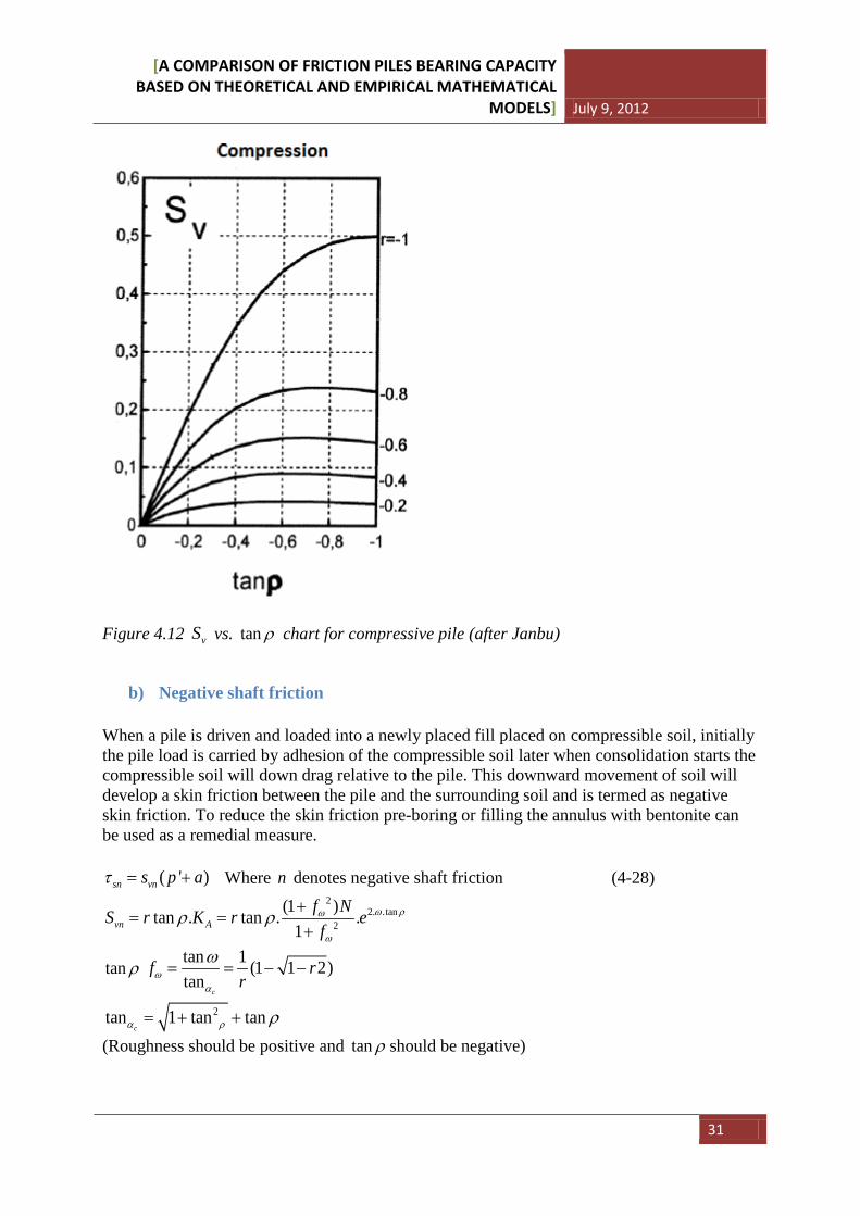
b) Negative shaft friction When a pile is driven and loaded into a newly placed fill placed on compressible soil, initially the pile load is carried by adhesion of the compressible soil later when consolidation starts the compressible soil will down drag relative to the pile. This downward movement of soil will develop a skin friction between the pile and the surrounding soil and is termed as negative skin friction. To reduce the skin friction pre-boring or filling the annulus with bentonite can be used as a remedial measure.
( ' )sn vns p aτ = + Where n denotes negative shaft friction (4-28) 2
2. .tan2
(1 )tan . tan . .1vn A
f NS r K r ef
ω ρω
ω
ρ ρ += =
+
tan ρtan 1 (1 1 2)tan
c
f rrω
α
ω= = − −
2tan 1 tan tancα ρ ρ= + +
(Roughness should be positive and tan ρ should be negative)
[A COMPARISON OF FRICTION PILES BEARING CAPACITY BASED ON THEORETICAL AND EMPIRICAL MATHEMATICAL
MODELS] July 9, 2012
32
Figure 4.13 vS vs. tan ρ chart for piles with negative skin friction (after Janbu)
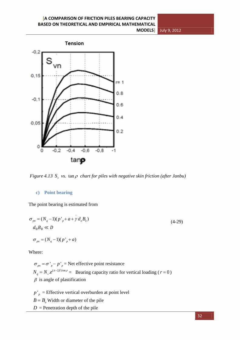
c) Point bearing The point bearing is estimated from
( 1)( ' )pn q p o oN p a d Bσ γ−
= − + + (4-29)
𝑑0𝐵0 ≪ 𝐷
( 1)( ' )pn q pN p aσ = − + Where: ' 'pn p ppσ σ= − = Net effective point resistance
( 2 ) tan.qN N e π β ρ−+= = Bearing capacity ratio for vertical loading ( 0r = )
β is angle of plastification
'pp = Effective vertical overburden at point level
oB B= Width or diameter of the pile D = Penetration depth of the pile
[A COMPARISON OF FRICTION PILES BEARING CAPACITY BASED ON THEORETICAL AND EMPIRICAL MATHEMATICAL
MODELS] July 9, 2012
33
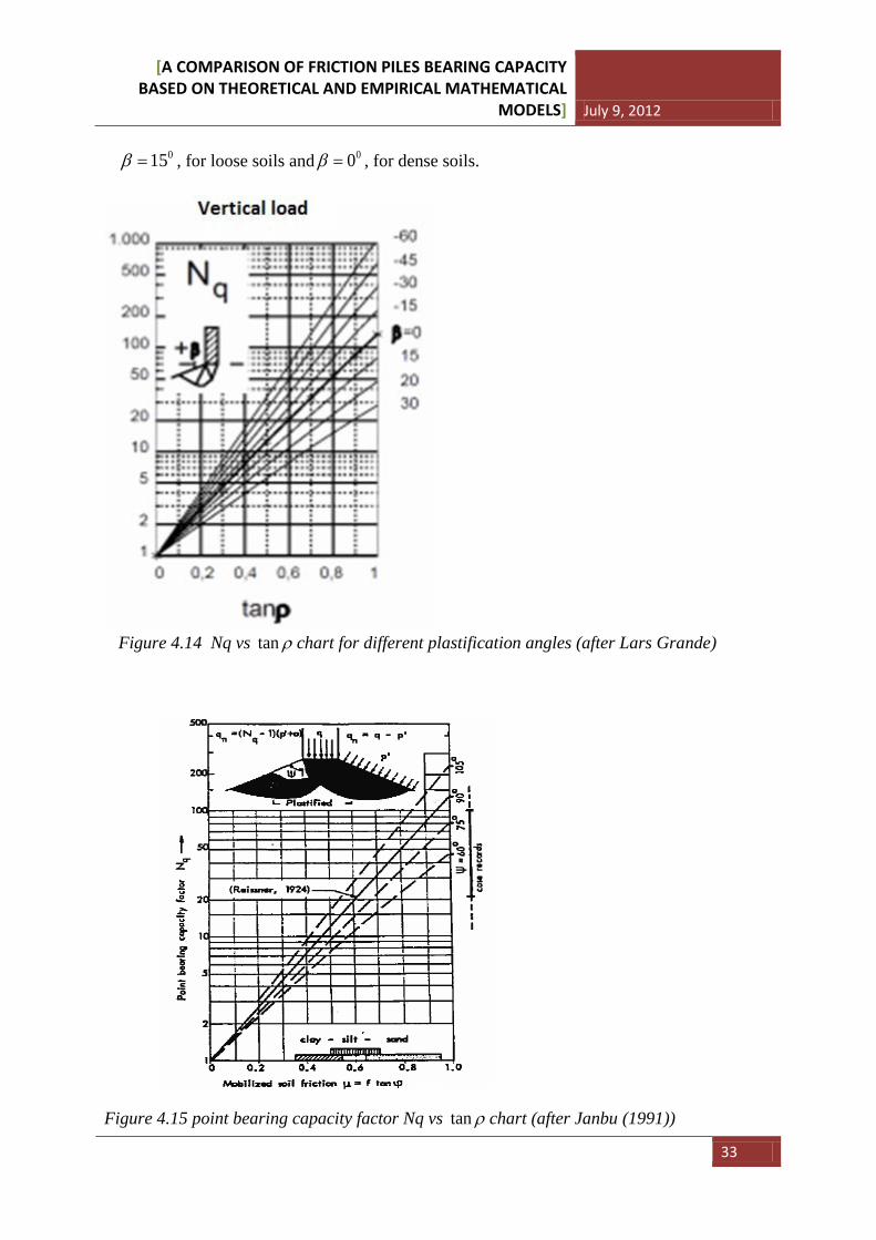
015β = , for loose soils and 00β = , for dense soils.
Figure 4.14 Nq vs tan ρ chart for different plastification angles (after Lars Grande)
Figure 4.15 point bearing capacity factor Nq vs tan ρ chart (after Janbu (1991))
[A COMPARISON OF FRICTION PILES BEARING CAPACITY BASED ON THEORETICAL AND EMPIRICAL MATHEMATICAL
MODELS] July 9, 2012
34
4.3 Effect of time on pile capacity
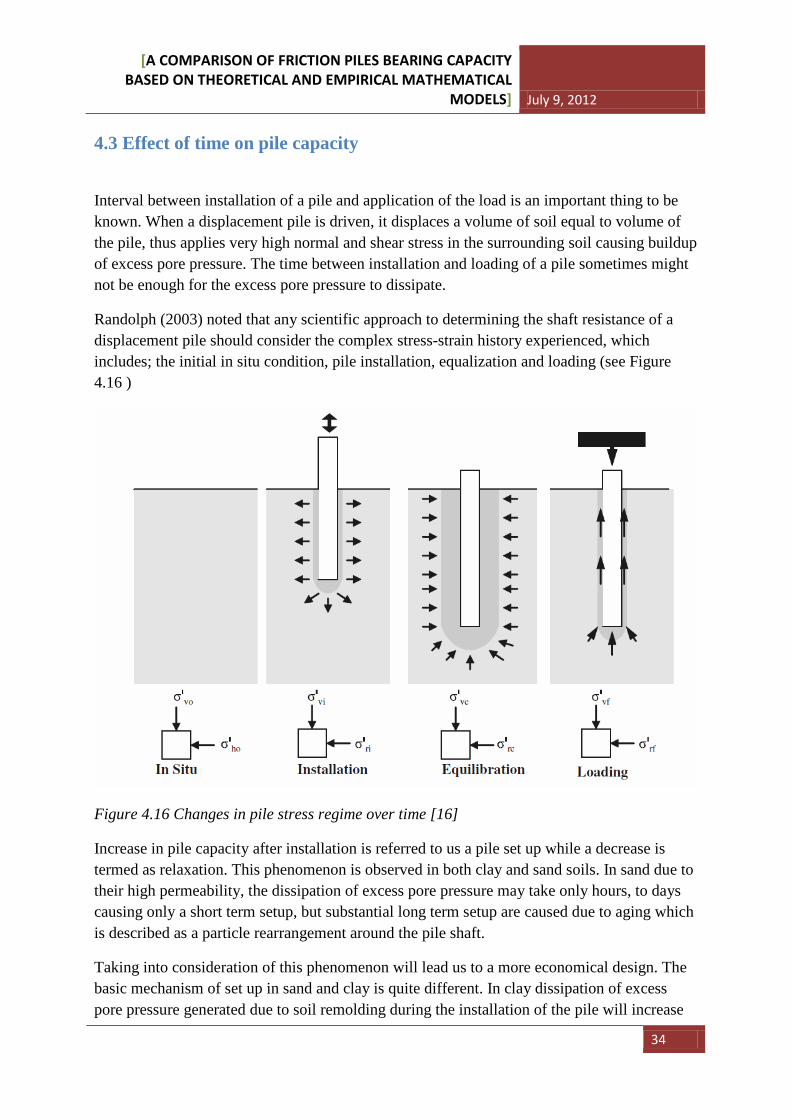
Interval between installation of a pile and application of the load is an important thing to be known. When a displacement pile is driven, it displaces a volume of soil equal to volume of the pile, thus applies very high normal and shear stress in the surrounding soil causing buildup of excess pore pressure. The time between installation and loading of a pile sometimes might not be enough for the excess pore pressure to dissipate.
Randolph (2003) noted that any scientific approach to determining the shaft resistance of a displacement pile should consider the complex stress-strain history experienced, which includes; the initial in situ condition, pile installation, equalization and loading (see Figure 4.16 )
Figure 4.16 Changes in pile stress regime over time [16]
Increase in pile capacity after installation is referred to us a pile set up while a decrease is termed as relaxation. This phenomenon is observed in both clay and sand soils. In sand due to their high permeability, the dissipation of excess pore pressure may take only hours, to days causing only a short term setup, but substantial long term setup are caused due to aging which is described as a particle rearrangement around the pile shaft.
Taking into consideration of this phenomenon will lead us to a more economical design. The basic mechanism of set up in sand and clay is quite different. In clay dissipation of excess pore pressure generated due to soil remolding during the installation of the pile will increase
[A COMPARISON OF FRICTION PILES BEARING CAPACITY BASED ON THEORETICAL AND EMPIRICAL MATHEMATICAL
MODELS] July 9, 2012
35
the radial effective stress of the soil which in turn increases the effective stress of the soil; consequently, the axial capacity of the pile will increase. In clay the dissipation of excess pore pressure will take months even years. In clay even after dissipation of excess pore water pressure, additional set up may occur at constant effective stress due to aging.
Chow believes the increase in shaft friction is unlikely from aging of sand or corrosion of steel piles, and he believes it is likely caused by relaxation of soil arched around the shaft, thereby increasing the radial stress at the interface [1]. Terzaghi and Peck noted that the carrying capacity decreases during the first two or three days after driving, this is due to it is probable, but not certain , that the high initial bearing capacity is due to a temporary state of stress that develops in the sand surrounding the point of the pile during driving [1]. The simplest way of modeling rate of pore pressure dissipation is using the radial consolidation theory and using this theory the time factor is given by the expression
𝑇 = 𝑡.𝑐ℎ𝑟02
(4-30)
Where
𝑇 = dimensionless time factor
𝑐ℎ = horizontal coefficient of consolidation
𝑡 = consolidation time
𝑟0 = outer pile radius
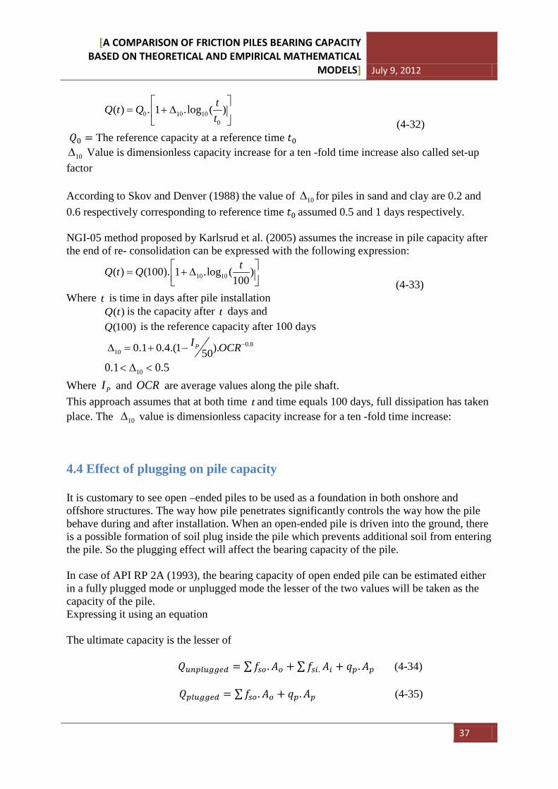
Using cavity expansion model based on the assumption of an ideal isotropic linear-elastic –perfectly-plastic (EP) type soil model the plasticized radius can be expressed in the following form [24]:
𝑟𝑝𝑟0
= �𝐺50𝑐𝑢
.�𝑟02−𝑟𝑖2
𝑟02 (4-31)
Where
𝑟𝑝 = radius of the plastic zone
𝑟𝑖 = inner pile radius
𝐺50 = shear modulus at 50% of maximum stress
𝑐𝑢 = undrained shear strength
[A COMPARISON OF FRICTION PILES BEARING CAPACITY BASED ON THEORETICAL AND EMPIRICAL MATHEMATICAL
MODELS] July 9, 2012
36
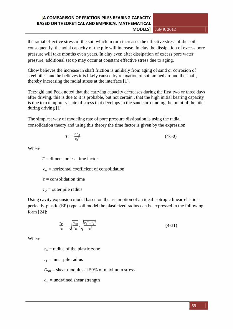
Figure 4.17 Time factors vs. degree of consolidation from linear radial consolidation theory of 1) ∆𝑢𝑖 decreases linearly with log (𝑟 𝑟0� ), 2) ∆𝑢𝑖 decreases linearly with (𝑟 𝑟0� ) (based on analytical results presented by Levadoux, 1982 and Chin, 1986) [24]
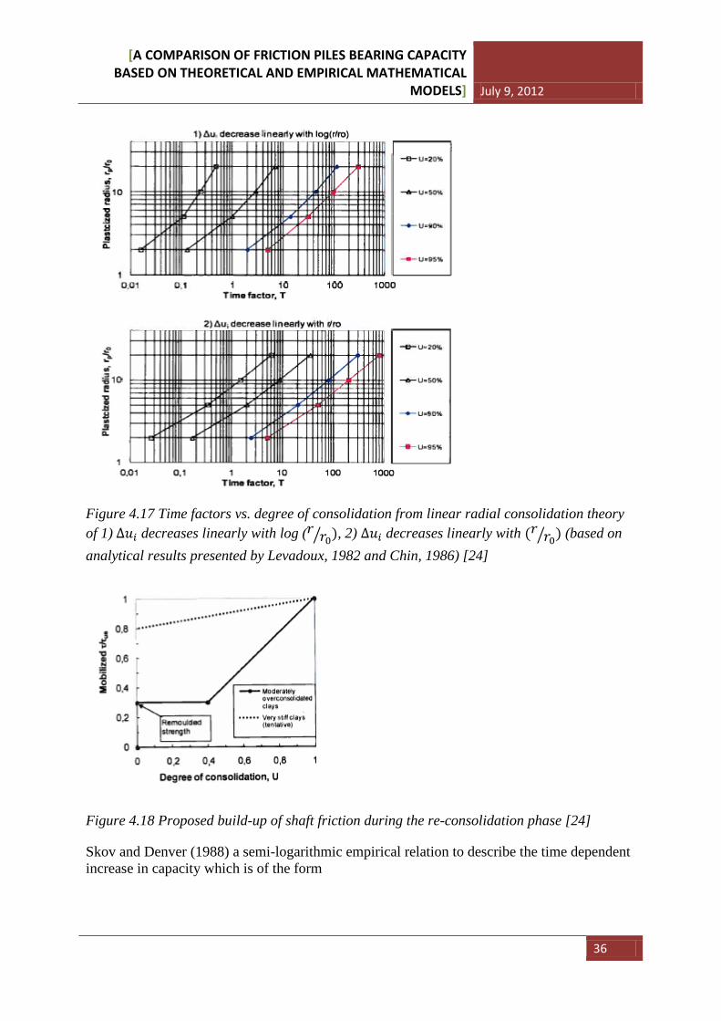
Figure 4.18 Proposed build-up of shaft friction during the re-consolidation phase [24]
Skov and Denver (1988) a semi-logarithmic empirical relation to describe the time dependent increase in capacity which is of the form
[A COMPARISON OF FRICTION PILES BEARING CAPACITY BASED ON THEORETICAL AND EMPIRICAL MATHEMATICAL
MODELS] July 9, 2012
37
0 10 100
( ) . 1 .log ( )tQ t Qt
= + ∆
(4-32)
𝑄0 = The reference capacity at a reference time 𝑡0
10∆ Value is dimensionless capacity increase for a ten -fold time increase also called set-up factor According to Skov and Denver (1988) the value of 10∆ for piles in sand and clay are 0.2 and 0.6 respectively corresponding to reference time 𝑡0 assumed 0.5 and 1 days respectively. NGI-05 method proposed by Karlsrud et al. (2005) assumes the increase in pile capacity after the end of re- consolidation can be expressed with the following expression:
10 10( ) (100). 1 .log ( )100
tQ t Q = + ∆ (4-33)
Where t is time in days after pile installation ( )Q t is the capacity after t days and (100)Q is the reference capacity after 100 days
0.810 0.1 0.4.(1 ).50
PI OCR−∆ = + −
100.1 0.5< ∆ < Where PI and OCR are average values along the pile shaft. This approach assumes that at both time t and time equals 100 days, full dissipation has taken place. The 10∆ value is dimensionless capacity increase for a ten -fold time increase:
4.4 Effect of plugging on pile capacity It is customary to see open –ended piles to be used as a foundation in both onshore and offshore structures. The way how pile penetrates significantly controls the way how the pile behave during and after installation. When an open-ended pile is driven into the ground, there is a possible formation of soil plug inside the pile which prevents additional soil from entering the pile. So the plugging effect will affect the bearing capacity of the pile. In case of API RP 2A (1993), the bearing capacity of open ended pile can be estimated either in a fully plugged mode or unplugged mode the lesser of the two values will be taken as the capacity of the pile. Expressing it using an equation The ultimate capacity is the lesser of 𝑄𝑢𝑛𝑝𝑙𝑢𝑔𝑔𝑒𝑑 = ∑𝑓𝑠𝑜 .𝐴𝑜 + ∑𝑓𝑠𝑖. 𝐴𝑖 + 𝑞𝑝.𝐴𝑝 (4-34) 𝑄𝑝𝑙𝑢𝑔𝑔𝑒𝑑 = ∑𝑓𝑠𝑜 .𝐴𝑜 + 𝑞𝑝.𝐴𝑝 (4-35)
[A COMPARISON OF FRICTION PILES BEARING CAPACITY BASED ON THEORETICAL AND EMPIRICAL MATHEMATICAL
MODELS] July 9, 2012
38
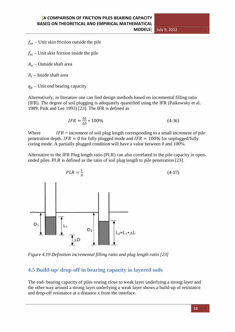
𝑓𝑠𝑜 – Unit skin friction outside the pile 𝑓𝑠𝑖 – Unit skin friction inside the pile 𝐴𝑜 – Outside shaft area 𝐴𝑖 – Inside shaft area 𝑞𝑝 – Unit end bearing capacity Alternatively, in literature one can find design methods based on incremental filling ratio (IFR). The degree of soil plugging is adequately quantified using the IFR (Paikowsky et al. 1989; Paik and Lee 1993) [23]. The IFR is defined as 𝐼𝐹𝑅 = ∆𝐿
∆𝐷∗ 100% (4-36)
Where 𝐼𝐹𝑅 = increment of soil plug length corresponding to a small increment of pile penetration depth. 𝐼𝐹𝑅 = 0 for fully plugged mode and 𝐼𝐹𝑅 = 100% for unplugged/fully coring mode. A partially plugged condition will have a value between 0 and 100%. Alternative to the IFR Plug length ratio (PLR) can also correlated to the pile capacity in open-ended piles. PLR is defined as the ratio of soil plug length to pile penetration [23]. 𝑃𝐿𝑅 = 𝐿
𝐷 (4-37)
Figure 4.19 Definition incremental filling ratio and plug length ratio [23]
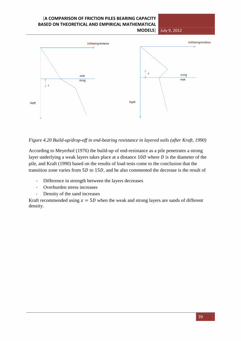
4.5 Build-up/ drop-off in bearing capacity in layered soils The end- bearing capacity of piles resting close to weak layer underlying a strong layer and the other way around a strong layer underlying a weak layer shows a build-up of resistance and drop-off resistance at a distance x from the interface.
[A COMPARISON OF FRICTION PILES BEARING CAPACITY BASED ON THEORETICAL AND EMPIRICAL MATHEMATICAL
MODELS] July 9, 2012
39
Figure 4.20 Build-up/drop-off in end-bearing resistance in layered soils (after Kraft, 1990)
According to Meyerhof (1976) the build-up of end-resistance as a pile penetrates a strong layer underlying a weak layers takes place at a distance 10𝐷 where 𝐷 is the diameter of the pile, and Kraft (1990) based on the results of load tests come to the conclusion that the transition zone varies from 5𝐷 to 15𝐷, and he also commented the decrease is the result of
- Difference in strength between the layers decreases - Overburden stress increases - Density of the sand increases
Kraft recommended using 𝑥 = 5𝐷 when the weak and strong layers are sands of different density.
[A COMPARISON OF FRICTION PILES BEARING CAPACITY BASED ON THEORETICAL AND EMPIRICAL MATHEMATICAL
MODELS] July 9, 2012
40
5 PILE DYNAMICS AND PILE LOAD TESTS
“The development of the wave equation analysis from the pre-computer era of the fifties (Smith 1960) to the advent of a computer version in the mid-seventies was a quantum leap in the foundation engineering. For the first time, a design could consider the entire pile driving system, such as wave propagation characteristics, velocity dependent aspects (damping), soil deformation characteristics, soil resistance (total as well as its distribution of resistance along the pile shaft and between the pile shaft and the pile toe), hammer behavior, and hammer cushion and pile cushion characteristics” [25].
5.1 Pile installation Piles are normally inserted into the ground using a hammer resting on the pile cap and there are different types of hammer exist today the simplest of them is the drop hammer, which is used for small projects and inaccessible conditions. The main disadvantage of using a drop hammer is the difficulty of controlling the drop height. Single acting hammer: they are also called compressed air hammers. The hammers are lifted up using steam or air pressure and drop using gravity. They operate at a rate up to 60 strokes per minute. They deliver slow blow rate, but still better blow rate than the drop hammers. Double acting hammers: These hammers use steam or compressed air both to lift the ram and drop it. Their ram weight generally ranging from 90kg-2300kg and rate of driving 300 blows per minute for light types. They are mainly used for sheet pile driving. According to Tomlinson (1995) one specific example of this hammer type is Vulcan 400C, with a ram mass of 18140kg and energy of 15660m/kg and driving rate of 100 blows per minute. Diesel hammer: This hammers work in a mechanism when the ram falls the air and the fuel compress and becomes hot this impact atomizes the diesel and result in explosion this explosion aids the hammer to drive the pile and to lift the ram as well. This hammer works pretty well in hard soils. They are easily moved from place to place and their fuel consumption is low. Jetting: High pressure water at pile point is sometimes used to assist driving. This method is normally used in sand or sandy gravel soils. Vibratory drivers: This method is best suited for driving sheet piles or bearing piles in sandy or gravelly soils. They have little use in stiff clays According to Bowles (1996) the three principal advantages of the vibratory drivers are the following.
1. Reduced driving vibrations 2. Reduced noise 3. Great speed of penetration-penetration rate up to 50mm/sec is possible.
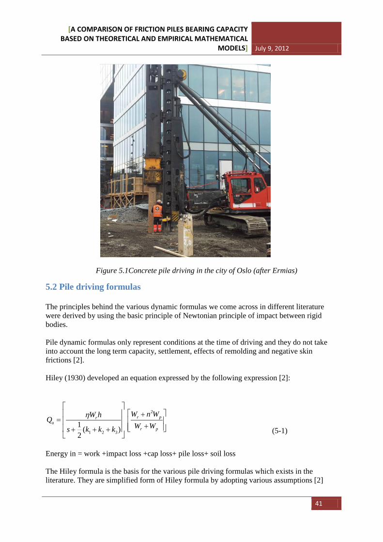
[A COMPARISON OF FRICTION PILES BEARING CAPACITY BASED ON THEORETICAL AND EMPIRICAL MATHEMATICAL
MODELS] July 9, 2012
41
Figure 5.1Concrete pile driving in the city of Oslo (after Ermias)
5.2 Pile driving formulas The principles behind the various dynamic formulas we come across in different literature were derived by using the basic principle of Newtonian principle of impact between rigid bodies. Pile dynamic formulas only represent conditions at the time of driving and they do not take into account the long term capacity, settlement, effects of remolding and negative skin frictions [2]. Hiley (1930) developed an equation expressed by the following expression [2]:
1 2 31 ( )2
ru
W hQs k k k
η
= + + +
2r p
r p
W n WW W
+
+ (5-1)
Energy in = work +impact loss +cap loss+ pile loss+ soil loss The Hiley formula is the basis for the various pile driving formulas which exists in the literature. They are simplified form of Hiley formula by adopting various assumptions [2]
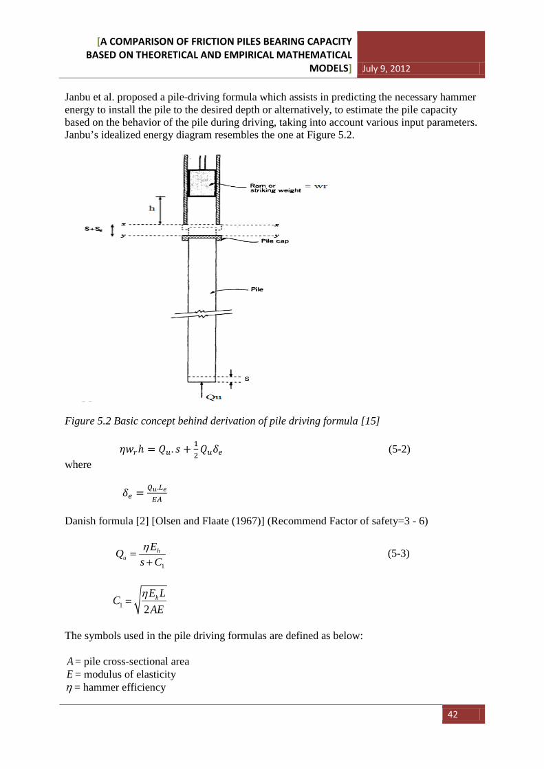
[A COMPARISON OF FRICTION PILES BEARING CAPACITY BASED ON THEORETICAL AND EMPIRICAL MATHEMATICAL
MODELS] July 9, 2012
42
Janbu et al. proposed a pile-driving formula which assists in predicting the necessary hammer energy to install the pile to the desired depth or alternatively, to estimate the pile capacity based on the behavior of the pile during driving, taking into account various input parameters. Janbu’s idealized energy diagram resembles the one at Figure 5.2.
Figure 5.2 Basic concept behind derivation of pile driving formula [15] 𝜂𝑤𝑟ℎ = 𝑄𝑢. 𝑠 + 1
2𝑄𝑢𝛿𝑒 (5-2)
where 𝛿𝑒 = 𝑄𝑢.𝐿𝑒
𝐸𝐴
Danish formula [2] [Olsen and Flaate (1967)] (Recommend Factor of safety=3 - 6)
1
hu
EQs Cη
=+
(5-3)
1 2
hE LCAE
η=
The symbols used in the pile driving formulas are defined as below: A = pile cross-sectional area E = modulus of elasticity η = hammer efficiency
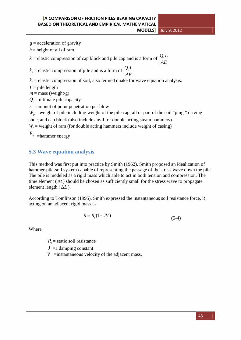
[A COMPARISON OF FRICTION PILES BEARING CAPACITY BASED ON THEORETICAL AND EMPIRICAL MATHEMATICAL
MODELS] July 9, 2012
43
g = acceleration of gravity h = height of all of ram
1k = elastic compression of cap block and pile cap and is a form of uQ LAE
2k = elastic compression of pile and is a form of uQ LAE
3k = elastic compression of soil, also termed quake for wave equation analysis. L = pile length m = mass (weight/g)
uQ = ultimate pile capacity s = amount of point penetration per blow
pW = weight of pile including weight of the pile cap, all or part of the soil “plug,” driving shoe, and cap block (also include anvil for double acting steam hammers)
rW = weight of ram (for double acting hammers include weight of casing)
hE =hammer energy
5.3 Wave equation analysis This method was first put into practice by Smith (1962). Smith proposed an idealization of hammer-pile-soil system capable of representing the passage of the stress wave down the pile. The pile is modeled as a rigid mass which able to act in both tension and compression. The time element ( t∆ ) should be chosen as sufficiently small for the stress wave to propagate element length ( L∆ ). According to Tomlinson (1995), Smith expressed the instantaneous soil resistance force, R, acting on an adjacent rigid mass as (1 )sR R JV= + (5-4) Where sR = static soil resistance J =a damping constant V =instantaneous velocity of the adjacent mass.
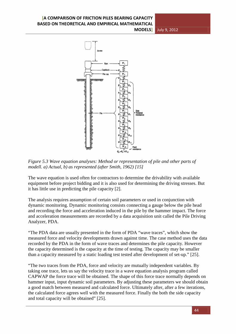
[A COMPARISON OF FRICTION PILES BEARING CAPACITY BASED ON THEORETICAL AND EMPIRICAL MATHEMATICAL
MODELS] July 9, 2012
44
Figure 5.3 Wave equation analyses: Method or representation of pile and other parts of modell. a) Actual, b) as represented (after Smith, 1962) [15] The wave equation is used often for contractors to determine the drivability with available equipment before project bidding and it is also used for determining the driving stresses. But it has little use in predicting the pile capacity [2]. The analysis requires assumption of certain soil parameters or used in conjunction with dynamic monitoring. Dynamic monitoring consists connecting a gauge below the pile head and recording the force and acceleration induced in the pile by the hammer impact. The force and acceleration measurements are recorded by a data acquisition unit called the Pile Driving Analyzer, PDA. “The PDA data are usually presented in the form of PDA “wave traces”, which show the measured force and velocity developments drawn against time. The case method uses the data recorded by the PDA in the form of wave traces and determines the pile capacity. However the capacity determined is the capacity at the time of testing. The capacity may be smaller than a capacity measured by a static loading test tested after development of set-up.” [25]. “The two traces from the PDA, force and velocity are mutually independent variables. By taking one trace, lets us say the velocity trace in a wave equation analysis program called CAPWAP the force trace will be obtained. The shape of this force trace normally depends on hammer input, input dynamic soil parameters. By adjusting these parameters we should obtain a good match between measured and calculated force. Ultimately after, after a few iterations, the calculated force agrees well with the measured force. Finally the both the side capacity and total capacity will be obtained” [25].
[A COMPARISON OF FRICTION PILES BEARING CAPACITY BASED ON THEORETICAL AND EMPIRICAL MATHEMATICAL
MODELS] July 9, 2012
45
“The capacity obtained by CAPWAP program is usually close to the capacity obtained from a static loading test. This doesn’t mean that the capacity is exactly the same. Even the capacity obtained by the static loading test varies with in 20% by the definition of the failure load.” [25].
5.4 Pile Load Tests The uncertainties in the sub surface soil properties in computation of capacity, uncertainties in using pile driving formulas and uncertainties using the wave equation lead us to perform a full-scale field load test. The load test is believed to be the most reliable method of computing the pile capacity. There are two broad types of pile load tests, namely the static pile load test and dynamic pile load test, but since the static load tests are traditionally used and perceived to show the long term sustained loading condition they are usually preferred to be used.
5.4.1 Static pile load test Despite the facts that load tests are the most time consuming and expensive to perform, they are the most accurate way of determining the ultimate compressive and tensile load capacities. Load tests are performed on piles to confirm results obtained by various methods such as laboratory testing methods, field investigations based methods, dynamic analysis based methods. Static load test involves assembling of a full- size prototype foundation then slowly loads it to failure. Practically load tests are performed on either on a test pile or a working pile. By definition, test piles are preliminary piles and during testing they are tested until failure and help to confirm the pile design. In the contrary, a working pile is one of the actual piles used and is tested until two times the design capacity. The test procedure is alike in both cases.
There are two ways of measuring the settlement. Namely, pile butt movement measurement and incremental strain measurement. The incremental strain measurement is used to address the distribution of load transfer from the pile to the soil and it can be optional.
Static loads were applied and maintained using a hydraulic jack and were measured with a load cell. Reaction to the jack load is provided by a steel frame that is attached to an array of steel H-piles located at least 3m away from the test pile.
Pile head deflections were measured relative to a fixed reference beam using dial gauges. Telltale measurements were made in reference to the pile head or the reference beam using dial gauges. Pile head and telltale deflection data were recorded for each loading increment.
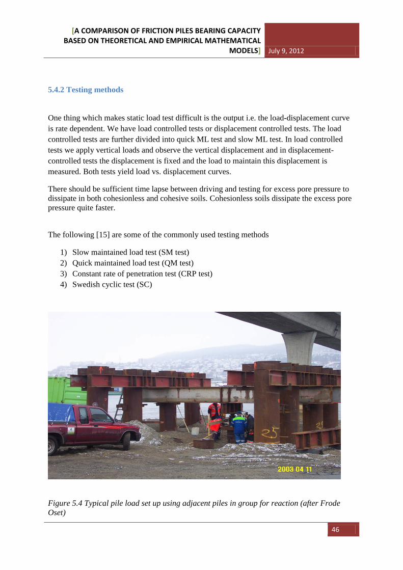
[A COMPARISON OF FRICTION PILES BEARING CAPACITY BASED ON THEORETICAL AND EMPIRICAL MATHEMATICAL
MODELS] July 9, 2012
46
5.4.2 Testing methods
One thing which makes static load test difficult is the output i.e. the load-displacement curve is rate dependent. We have load controlled tests or displacement controlled tests. The load controlled tests are further divided into quick ML test and slow ML test. In load controlled tests we apply vertical loads and observe the vertical displacement and in displacement-controlled tests the displacement is fixed and the load to maintain this displacement is measured. Both tests yield load vs. displacement curves.
There should be sufficient time lapse between driving and testing for excess pore pressure to dissipate in both cohesionless and cohesive soils. Cohesionless soils dissipate the excess pore pressure quite faster.
The following [15] are some of the commonly used testing methods
1) Slow maintained load test (SM test) 2) Quick maintained load test (QM test) 3) Constant rate of penetration test (CRP test) 4) Swedish cyclic test (SC)
Figure 5.4 Typical pile load set up using adjacent piles in group for reaction (after Frode Oset)
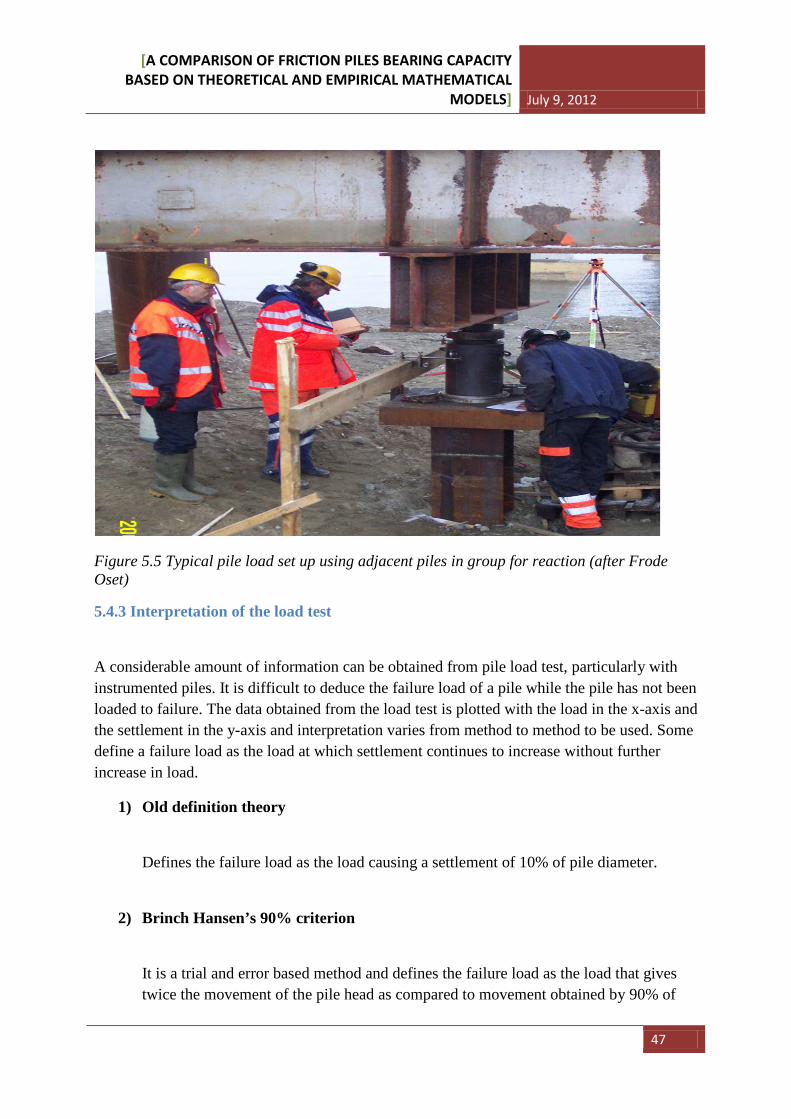
[A COMPARISON OF FRICTION PILES BEARING CAPACITY BASED ON THEORETICAL AND EMPIRICAL MATHEMATICAL
MODELS] July 9, 2012
47
Figure 5.5 Typical pile load set up using adjacent piles in group for reaction (after Frode Oset)
5.4.3 Interpretation of the load test
A considerable amount of information can be obtained from pile load test, particularly with instrumented piles. It is difficult to deduce the failure load of a pile while the pile has not been loaded to failure. The data obtained from the load test is plotted with the load in the x-axis and the settlement in the y-axis and interpretation varies from method to method to be used. Some define a failure load as the load at which settlement continues to increase without further increase in load.
1) Old definition theory
Defines the failure load as the load causing a settlement of 10% of pile diameter.
2) Brinch Hansen’s 90% criterion
It is a trial and error based method and defines the failure load as the load that gives twice the movement of the pile head as compared to movement obtained by 90% of
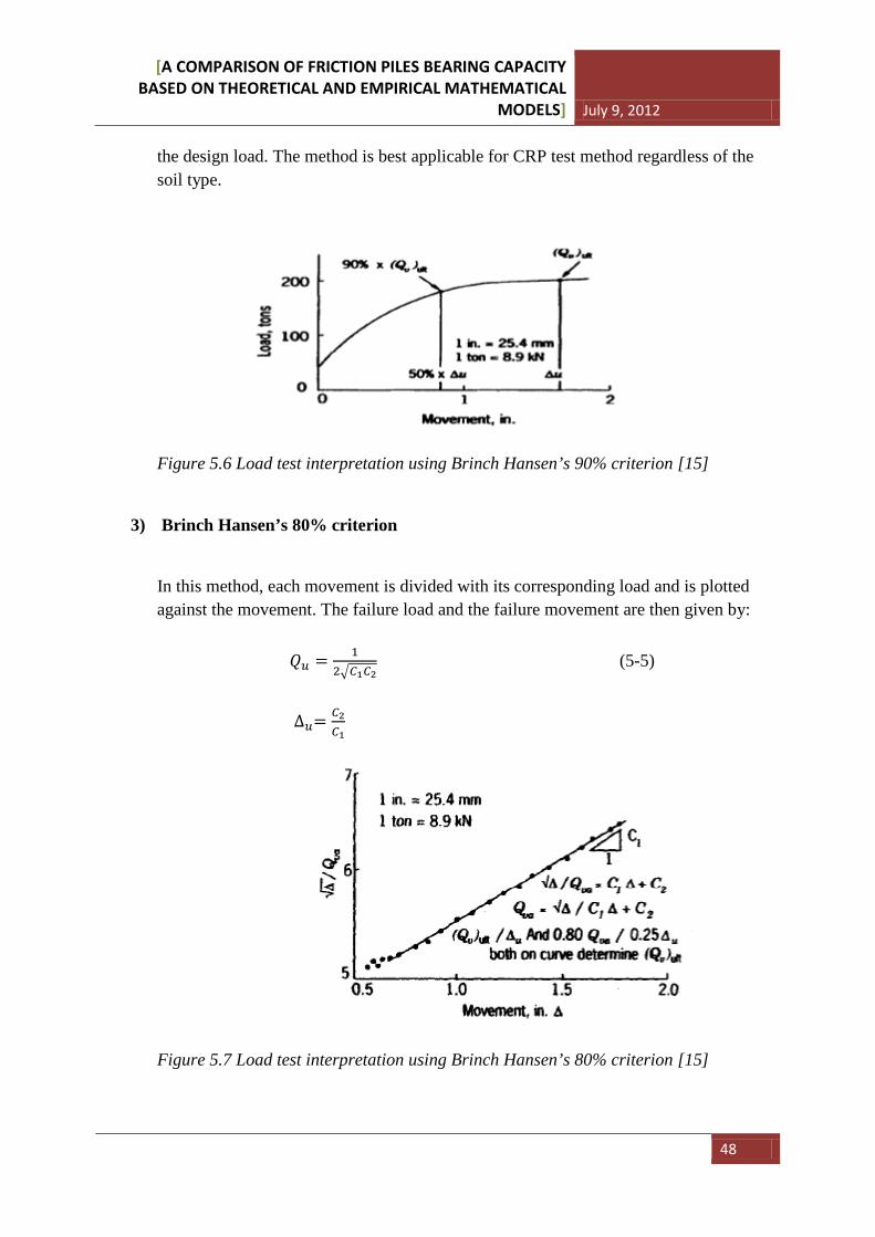
[A COMPARISON OF FRICTION PILES BEARING CAPACITY BASED ON THEORETICAL AND EMPIRICAL MATHEMATICAL
MODELS] July 9, 2012
48
the design load. The method is best applicable for CRP test method regardless of the soil type.
Figure 5.6 Load test interpretation using Brinch Hansen’s 90% criterion [15]
3) Brinch Hansen’s 80% criterion
In this method, each movement is divided with its corresponding load and is plotted against the movement. The failure load and the failure movement are then given by: 𝑄𝑢 = 1
2�𝐶1𝐶2 (5-5)
∆𝑢= 𝐶2
𝐶1
Figure 5.7 Load test interpretation using Brinch Hansen’s 80% criterion [15]
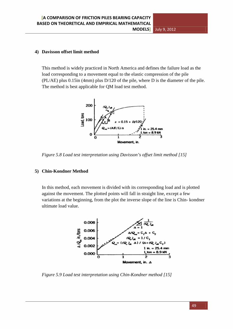
[A COMPARISON OF FRICTION PILES BEARING CAPACITY BASED ON THEORETICAL AND EMPIRICAL MATHEMATICAL
MODELS] July 9, 2012
49
4) Davisson offset limit method
This method is widely practiced in North America and defines the failure load as the load corresponding to a movement equal to the elastic compression of the pile (PL/AE) plus 0.15in (4mm) plus D/120 of the pile, where D is the diameter of the pile. The method is best applicable for QM load test method.
Figure 5.8 Load test interpretation using Davisson’s offset limit method [15]
5) Chin-Kondner Method
In this method, each movement is divided with its corresponding load and is plotted against the movement. The plotted points will fall in straight line, except a few variations at the beginning, from the plot the inverse slope of the line is Chin- kondner ultimate load value.
Figure 5.9 Load test interpretation using Chin-Kondner method [15]
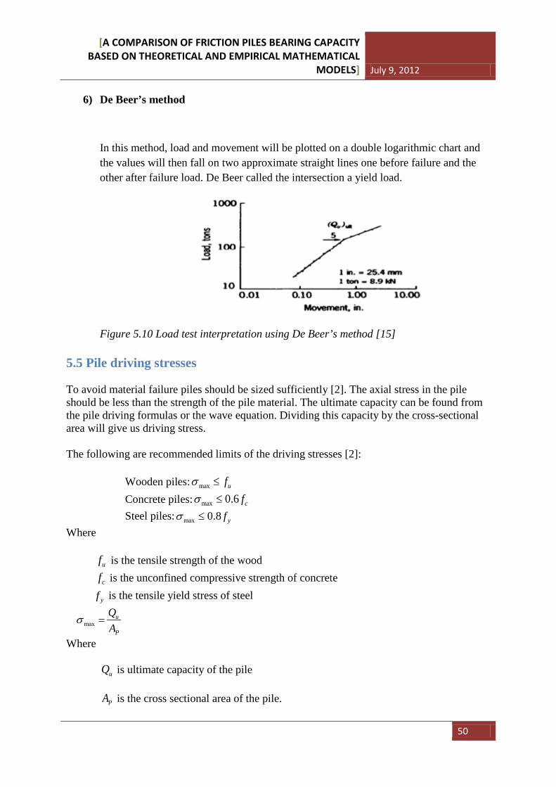
[A COMPARISON OF FRICTION PILES BEARING CAPACITY BASED ON THEORETICAL AND EMPIRICAL MATHEMATICAL
MODELS] July 9, 2012
50
6) De Beer’s method
In this method, load and movement will be plotted on a double logarithmic chart and the values will then fall on two approximate straight lines one before failure and the other after failure load. De Beer called the intersection a yield load.
Figure 5.10 Load test interpretation using De Beer’s method [15] 5.5 Pile driving stresses To avoid material failure piles should be sized sufficiently [2]. The axial stress in the pile should be less than the strength of the pile material. The ultimate capacity can be found from the pile driving formulas or the wave equation. Dividing this capacity by the cross-sectional area will give us driving stress. The following are recommended limits of the driving stresses [2]: Wooden piles: max ufσ ≤ Concrete piles: max 0.6 cfσ ≤ Steel piles: max 0.8 yfσ ≤ Where uf is the tensile strength of the wood cf is the unconfined compressive strength of concrete
yf is the tensile yield stress of steel
maxu
P
QA
σ =
Where
uQ is ultimate capacity of the pile
PA is the cross sectional area of the pile.
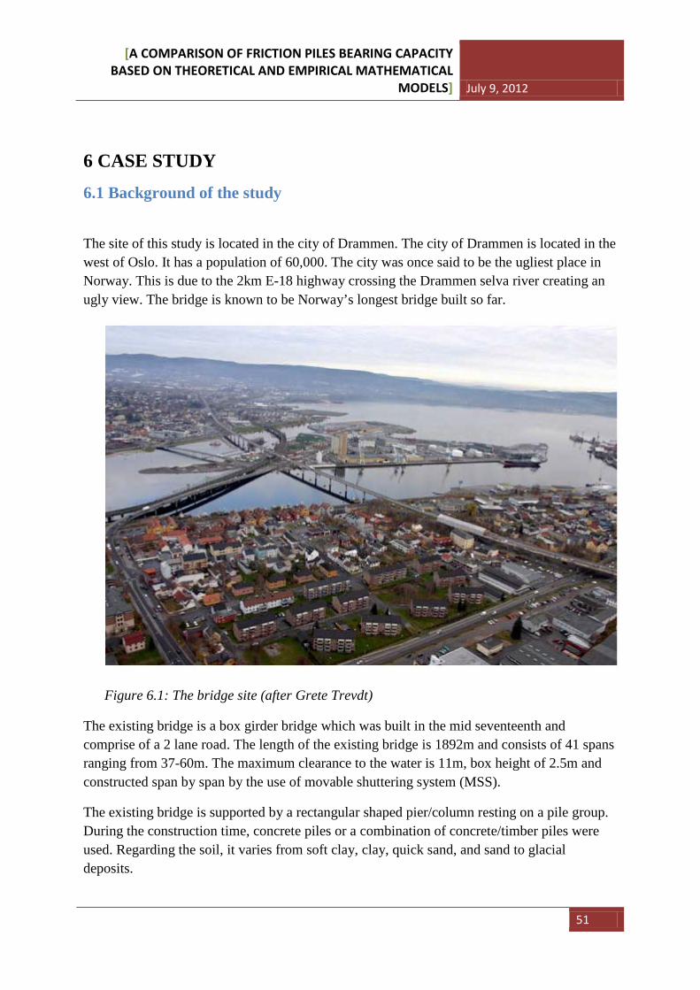
[A COMPARISON OF FRICTION PILES BEARING CAPACITY BASED ON THEORETICAL AND EMPIRICAL MATHEMATICAL
MODELS] July 9, 2012
51
6 CASE STUDY
6.1 Background of the study
The site of this study is located in the city of Drammen. The city of Drammen is located in the west of Oslo. It has a population of 60,000. The city was once said to be the ugliest place in Norway. This is due to the 2km E-18 highway crossing the Drammen selva river creating an ugly view. The bridge is known to be Norway’s longest bridge built so far.
Figure 6.1: The bridge site (after Grete Trevdt)
The existing bridge is a box girder bridge which was built in the mid seventeenth and comprise of a 2 lane road. The length of the existing bridge is 1892m and consists of 41 spans ranging from 37-60m. The maximum clearance to the water is 11m, box height of 2.5m and constructed span by span by the use of movable shuttering system (MSS).
The existing bridge is supported by a rectangular shaped pier/column resting on a pile group. During the construction time, concrete piles or a combination of concrete/timber piles were used. Regarding the soil, it varies from soft clay, clay, quick sand, and sand to glacial deposits.
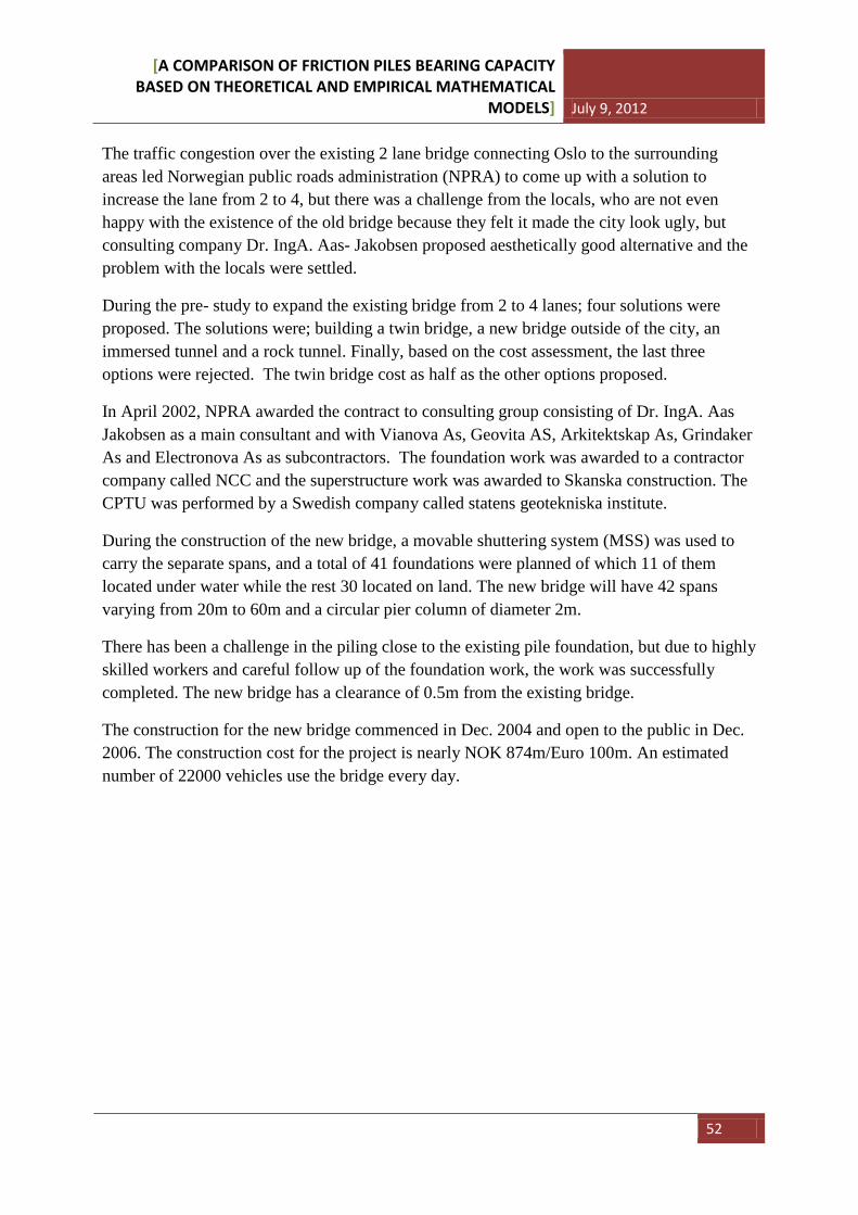
[A COMPARISON OF FRICTION PILES BEARING CAPACITY BASED ON THEORETICAL AND EMPIRICAL MATHEMATICAL
MODELS] July 9, 2012
52
The traffic congestion over the existing 2 lane bridge connecting Oslo to the surrounding areas led Norwegian public roads administration (NPRA) to come up with a solution to increase the lane from 2 to 4, but there was a challenge from the locals, who are not even happy with the existence of the old bridge because they felt it made the city look ugly, but consulting company Dr. IngA. Aas- Jakobsen proposed aesthetically good alternative and the problem with the locals were settled.
During the pre- study to expand the existing bridge from 2 to 4 lanes; four solutions were proposed. The solutions were; building a twin bridge, a new bridge outside of the city, an immersed tunnel and a rock tunnel. Finally, based on the cost assessment, the last three options were rejected. The twin bridge cost as half as the other options proposed.
In April 2002, NPRA awarded the contract to consulting group consisting of Dr. IngA. Aas Jakobsen as a main consultant and with Vianova As, Geovita AS, Arkitektskap As, Grindaker As and Electronova As as subcontractors. The foundation work was awarded to a contractor company called NCC and the superstructure work was awarded to Skanska construction. The CPTU was performed by a Swedish company called statens geotekniska institute.
During the construction of the new bridge, a movable shuttering system (MSS) was used to carry the separate spans, and a total of 41 foundations were planned of which 11 of them located under water while the rest 30 located on land. The new bridge will have 42 spans varying from 20m to 60m and a circular pier column of diameter 2m.
There has been a challenge in the piling close to the existing pile foundation, but due to highly skilled workers and careful follow up of the foundation work, the work was successfully completed. The new bridge has a clearance of 0.5m from the existing bridge.
The construction for the new bridge commenced in Dec. 2004 and open to the public in Dec. 2006. The construction cost for the project is nearly NOK 874m/Euro 100m. An estimated number of 22000 vehicles use the bridge every day.
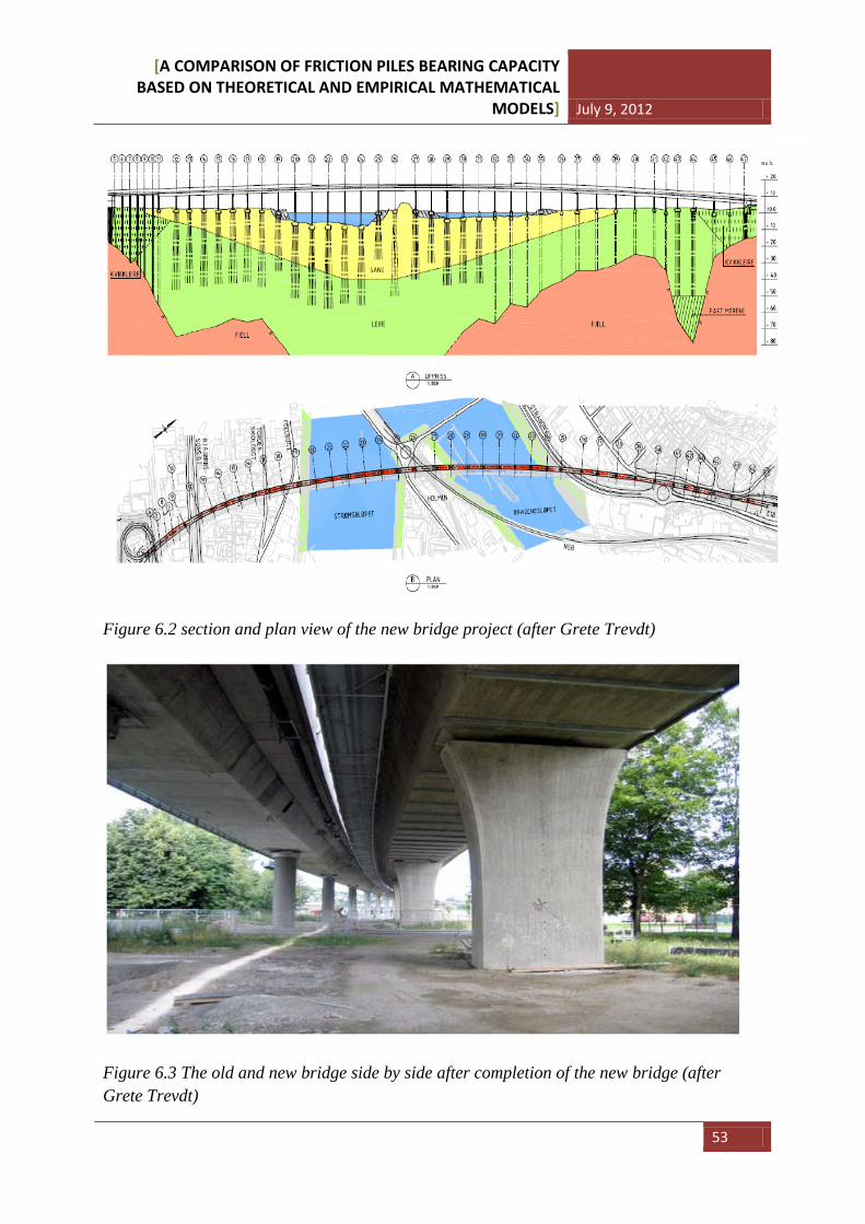
[A COMPARISON OF FRICTION PILES BEARING CAPACITY BASED ON THEORETICAL AND EMPIRICAL MATHEMATICAL
MODELS] July 9, 2012
53
Figure 6.2 section and plan view of the new bridge project (after Grete Trevdt)
Figure 6.3 The old and new bridge side by side after completion of the new bridge (after Grete Trevdt)
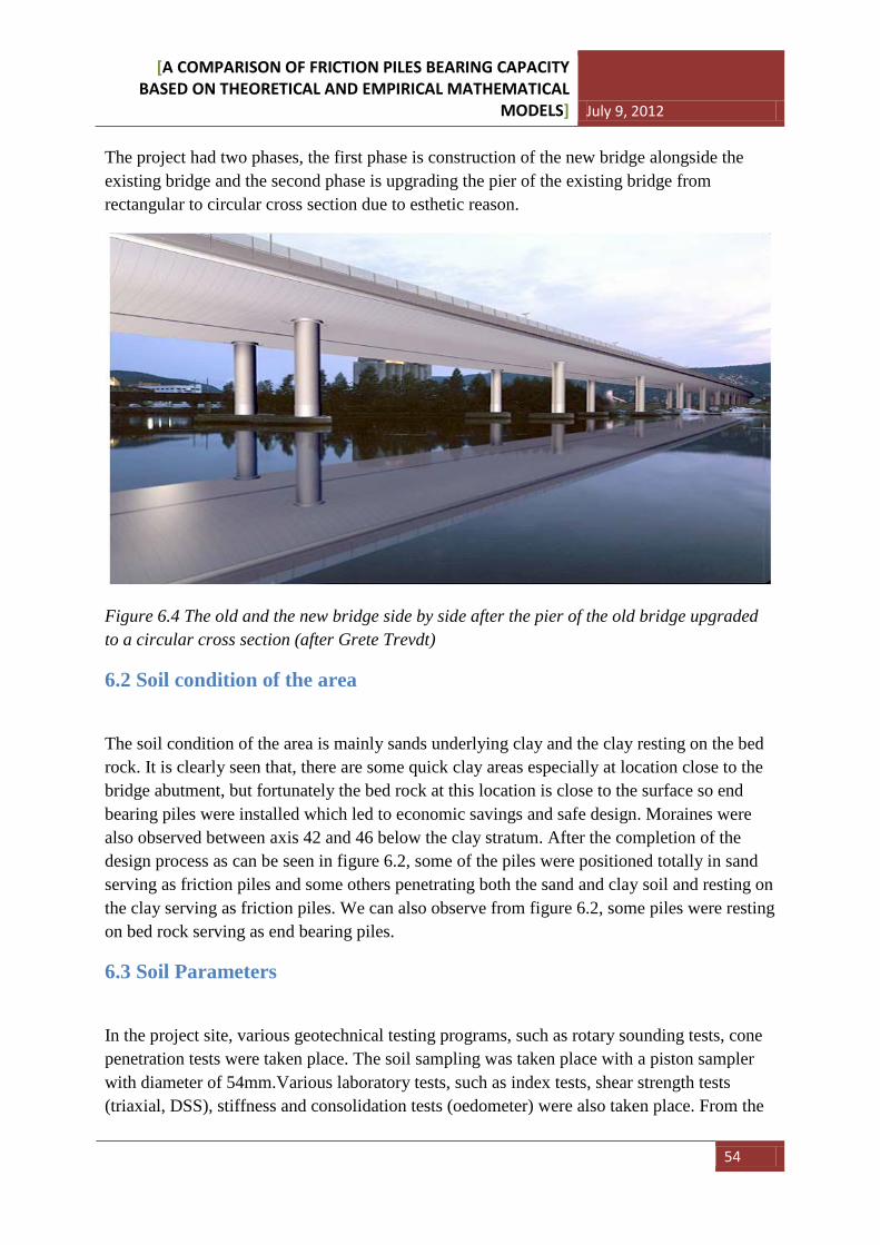
[A COMPARISON OF FRICTION PILES BEARING CAPACITY BASED ON THEORETICAL AND EMPIRICAL MATHEMATICAL
MODELS] July 9, 2012
54
The project had two phases, the first phase is construction of the new bridge alongside the existing bridge and the second phase is upgrading the pier of the existing bridge from rectangular to circular cross section due to esthetic reason.
Figure 6.4 The old and the new bridge side by side after the pier of the old bridge upgraded to a circular cross section (after Grete Trevdt)
6.2 Soil condition of the area
The soil condition of the area is mainly sands underlying clay and the clay resting on the bed rock. It is clearly seen that, there are some quick clay areas especially at location close to the bridge abutment, but fortunately the bed rock at this location is close to the surface so end bearing piles were installed which led to economic savings and safe design. Moraines were also observed between axis 42 and 46 below the clay stratum. After the completion of the design process as can be seen in figure 6.2, some of the piles were positioned totally in sand serving as friction piles and some others penetrating both the sand and clay soil and resting on the clay serving as friction piles. We can also observe from figure 6.2, some piles were resting on bed rock serving as end bearing piles.
6.3 Soil Parameters
In the project site, various geotechnical testing programs, such as rotary sounding tests, cone penetration tests were taken place. The soil sampling was taken place with a piston sampler with diameter of 54mm.Various laboratory tests, such as index tests, shear strength tests (triaxial, DSS), stiffness and consolidation tests (oedometer) were also taken place. From the
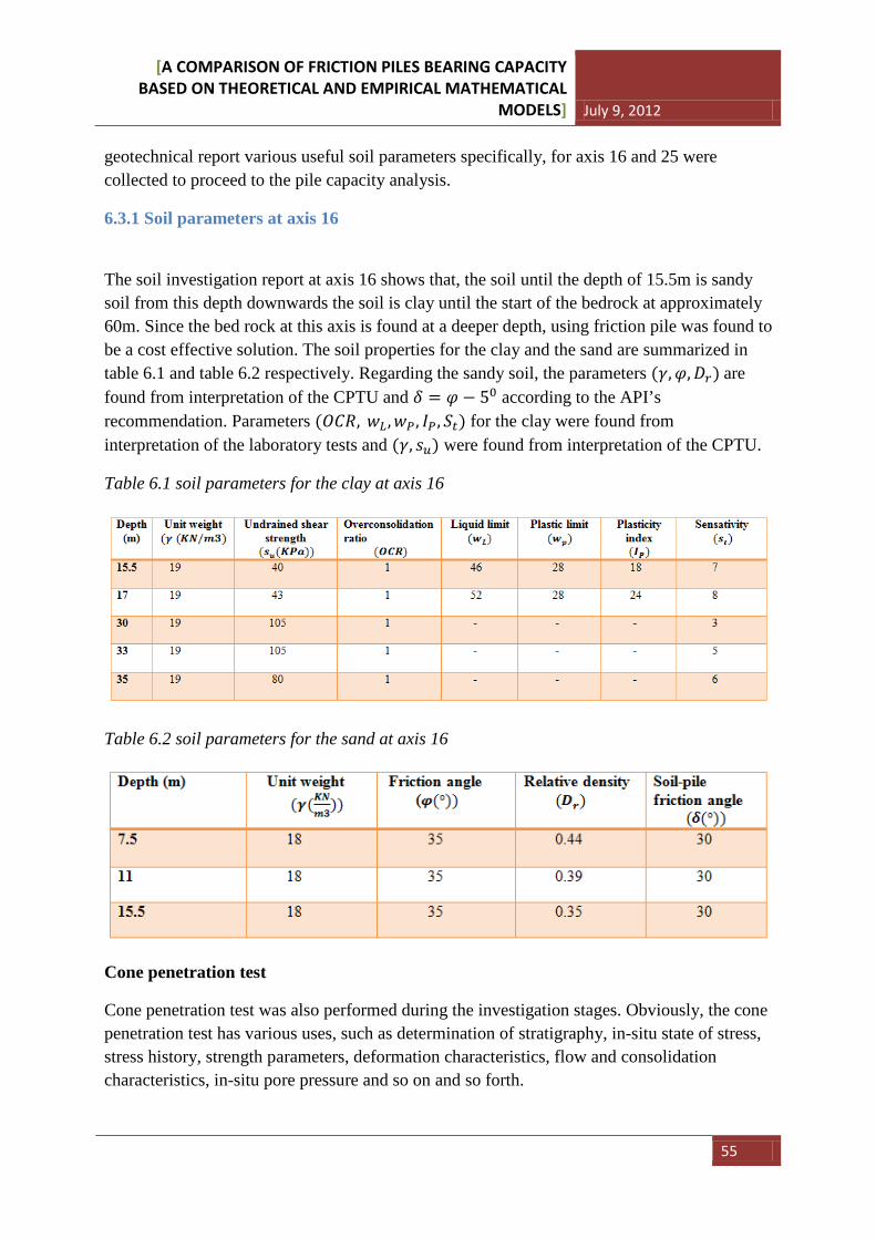
[A COMPARISON OF FRICTION PILES BEARING CAPACITY BASED ON THEORETICAL AND EMPIRICAL MATHEMATICAL
MODELS] July 9, 2012
55
geotechnical report various useful soil parameters specifically, for axis 16 and 25 were collected to proceed to the pile capacity analysis.
6.3.1 Soil parameters at axis 16
The soil investigation report at axis 16 shows that, the soil until the depth of 15.5m is sandy soil from this depth downwards the soil is clay until the start of the bedrock at approximately 60m. Since the bed rock at this axis is found at a deeper depth, using friction pile was found to be a cost effective solution. The soil properties for the clay and the sand are summarized in table 6.1 and table 6.2 respectively. Regarding the sandy soil, the parameters (𝛾,𝜑,𝐷𝑟) are found from interpretation of the CPTU and 𝛿 = 𝜑 − 50 according to the API’s recommendation. Parameters (𝑂𝐶𝑅, 𝑤𝐿 ,𝑤𝑃, 𝐼𝑃, 𝑆𝑡) for the clay were found from interpretation of the laboratory tests and (𝛾, 𝑠𝑢) were found from interpretation of the CPTU.
Table 6.1 soil parameters for the clay at axis 16
Table 6.2 soil parameters for the sand at axis 16
Cone penetration test
Cone penetration test was also performed during the investigation stages. Obviously, the cone penetration test has various uses, such as determination of stratigraphy, in-situ state of stress, stress history, strength parameters, deformation characteristics, flow and consolidation characteristics, in-situ pore pressure and so on and so forth.
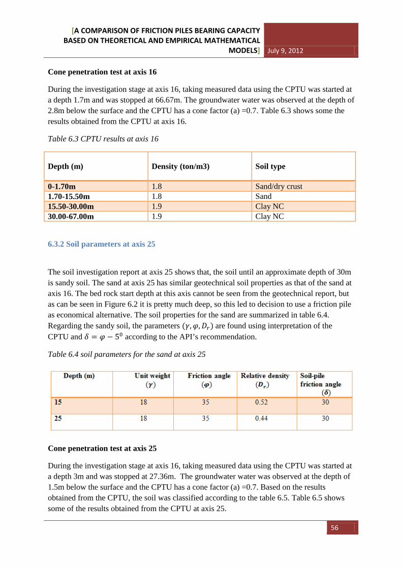
[A COMPARISON OF FRICTION PILES BEARING CAPACITY BASED ON THEORETICAL AND EMPIRICAL MATHEMATICAL
MODELS] July 9, 2012
56
Cone penetration test at axis 16
During the investigation stage at axis 16, taking measured data using the CPTU was started at a depth 1.7m and was stopped at 66.67m. The groundwater water was observed at the depth of 2.8m below the surface and the CPTU has a cone factor (a) =0.7. Table 6.3 shows some the results obtained from the CPTU at axis 16.
Table 6.3 CPTU results at axis 16
Depth (m)
Density (ton/m3)
Soil type
0-1.70m 1.8 Sand/dry crust 1.70-15.50m 1.8 Sand 15.50-30.00m 1.9 Clay NC 30.00-67.00m 1.9 Clay NC
6.3.2 Soil parameters at axis 25
The soil investigation report at axis 25 shows that, the soil until an approximate depth of 30m is sandy soil. The sand at axis 25 has similar geotechnical soil properties as that of the sand at axis 16. The bed rock start depth at this axis cannot be seen from the geotechnical report, but as can be seen in Figure 6.2 it is pretty much deep, so this led to decision to use a friction pile as economical alternative. The soil properties for the sand are summarized in table 6.4. Regarding the sandy soil, the parameters (𝛾,𝜑,𝐷𝑟) are found using interpretation of the CPTU and 𝛿 = 𝜑 − 50 according to the API’s recommendation.
Table 6.4 soil parameters for the sand at axis 25
Cone penetration test at axis 25
During the investigation stage at axis 16, taking measured data using the CPTU was started at a depth 3m and was stopped at 27.36m. The groundwater water was observed at the depth of 1.5m below the surface and the CPTU has a cone factor (a) =0.7. Based on the results obtained from the CPTU, the soil was classified according to the table 6.5. Table 6.5 shows some of the results obtained from the CPTU at axis 25.
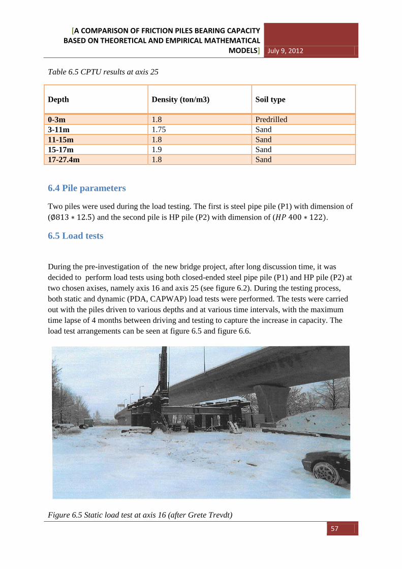
[A COMPARISON OF FRICTION PILES BEARING CAPACITY BASED ON THEORETICAL AND EMPIRICAL MATHEMATICAL
MODELS] July 9, 2012
57
Table 6.5 CPTU results at axis 25
Depth
Density (ton/m3)
Soil type
0-3m 1.8 Predrilled 3-11m 1.75 Sand 11-15m 1.8 Sand 15-17m 1.9 Sand 17-27.4m 1.8 Sand
6.4 Pile parameters
Two piles were used during the load testing. The first is steel pipe pile (P1) with dimension of (∅813 ∗ 12.5) and the second pile is HP pile (P2) with dimension of (𝐻𝑃 400 ∗ 122).
6.5 Load tests
During the pre-investigation of the new bridge project, after long discussion time, it was decided to perform load tests using both closed-ended steel pipe pile (P1) and HP pile (P2) at two chosen axises, namely axis 16 and axis 25 (see figure 6.2). During the testing process, both static and dynamic (PDA, CAPWAP) load tests were performed. The tests were carried out with the piles driven to various depths and at various time intervals, with the maximum time lapse of 4 months between driving and testing to capture the increase in capacity. The load test arrangements can be seen at figure 6.5 and figure 6.6.
Figure 6.5 Static load test at axis 16 (after Grete Trevdt)
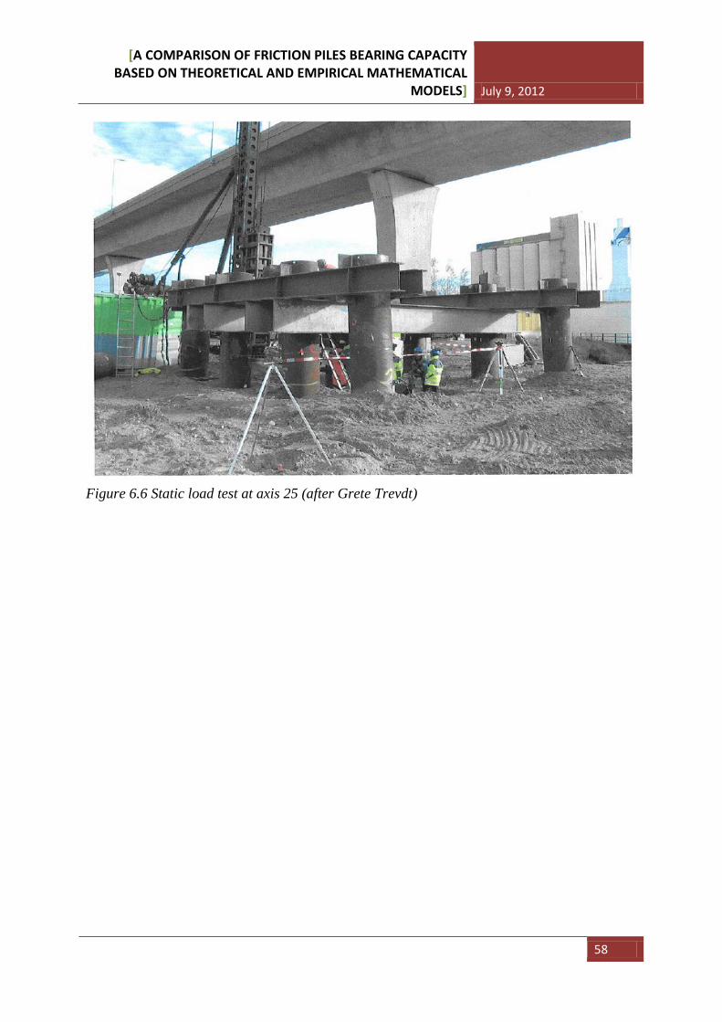
[A COMPARISON OF FRICTION PILES BEARING CAPACITY BASED ON THEORETICAL AND EMPIRICAL MATHEMATICAL
MODELS] July 9, 2012
58
Figure 6.6 Static load test at axis 25 (after Grete Trevdt)
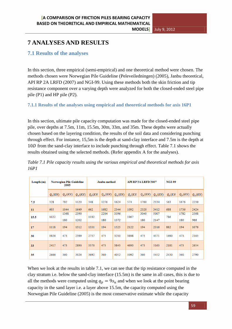
[A COMPARISON OF FRICTION PILES BEARING CAPACITY BASED ON THEORETICAL AND EMPIRICAL MATHEMATICAL
MODELS] July 9, 2012
59
7 ANALYSES AND RESULTS
7.1 Results of the analyses
In this section, three empirical (semi-empirical) and one theoretical method were chosen. The methods chosen were Norwegian Pile Guideline (Peleveiledningen) (2005), Janbu theoretical, API RP 2A LRFD (2007) and NGI-99. Using these methods both the skin friction and tip resistance component over a varying depth were analyzed for both the closed-ended steel pipe pile (P1) and HP pile (P2).
7.1.1 Results of the analyses using empirical and theoretical methods for axis 16P1
In this section, ultimate pile capacity computation was made for the closed-ended steel pipe pile, over depths at 7.5m, 11m, 15.5m, 30m, 33m, and 35m. These depths were actually chosen based on the layering condition, the results of the soil data and considering punching through effect. For instance, 15,5m is the depth at sand-clay interface and 7.5m is the depth at 10𝐷 from the sand-clay interface to include punching through effect. Table 7.1 shows the results obtained using the selected methods. (Refer appendix A for the analyses).
Table 7.1 Pile capacity results using the various empirical and theoretical methods for axis 16P1
When we look at the results in table 7.1, we can see that the tip resistance computed in the clay stratum i.e. below the sand-clay interface (15.5m) is the same in all cases, this is due to all the methods were computed using 𝑞𝑝 = 9𝑠𝑢 and when we look at the point bearing capacity in the sand layer i.e. a layer above 15.5m, the capacity computed using the Norwegian Pile Guideline (2005) is the most conservative estimate while the capacity
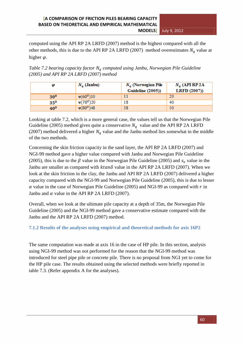
[A COMPARISON OF FRICTION PILES BEARING CAPACITY BASED ON THEORETICAL AND EMPIRICAL MATHEMATICAL
MODELS] July 9, 2012
60
computed using the API RP 2A LRFD (2007) method is the highest compared with all the other methods, this is due to the API RP 2A LRFD (2007) method overestimates 𝑁𝑞 value at higher 𝜑.
Table 7.2 bearing capacity factor 𝑁𝑞 computed using Janbu, Norwegian Pile Guideline (2005) and API RP 2A LRFD (2007) method
Looking at table 7.2, which is a more general case, the values tell us that the Norwegian Pile Guideline (2005) method gives quite a conservative 𝑁𝑞 value and the API RP 2A LRFD (2007) method delivered a higher 𝑁𝑞 value and the Janbu method lies somewhat in the middle of the two methods.
Concerning the skin friction capacity in the sand layer, the API RP 2A LRFD (2007) and NGI-99 method gave a higher value compared with Janbu and Norwegian Pile Guideline (2005), this is due to the 𝛽 value in the Norwegian Pile Guideline (2005) and 𝑠𝑣 value in the Janbu are smaller as compared with 𝑘𝑡𝑎𝑛𝛿 value in the API RP 2A LRFD (2007). When we look at the skin friction in the clay, the Janbu and API RP 2A LRFD (2007) delivered a higher capacity compared with the NGI-99 and Norwegian Pile Guideline (2005), this is due to lesser 𝛼 value in the case of Norwegian Pile Guideline (2005) and NGI-99 as compared with 𝑟 in Janbu and 𝛼 value in the API RP 2A LRFD (2007).
Overall, when we look at the ultimate pile capacity at a depth of 35m, the Norwegian Pile Guideline (2005) and the NGI-99 method gave a conservative estimate compared with the Janbu and the API RP 2A LRFD (2007) method.
7.1.2 Results of the analyses using empirical and theoretical methods for axis 16P2
The same computation was made at axis 16 in the case of HP pile. In this section, analysis using NGI-99 method was not performed for the reason that the NGI-99 method was introduced for steel pipe pile or concrete pile. There is no proposal from NGI yet to come for the HP pile case. The results obtained using the selected methods were briefly reported in table 7.3. (Refer appendix A for the analyses).
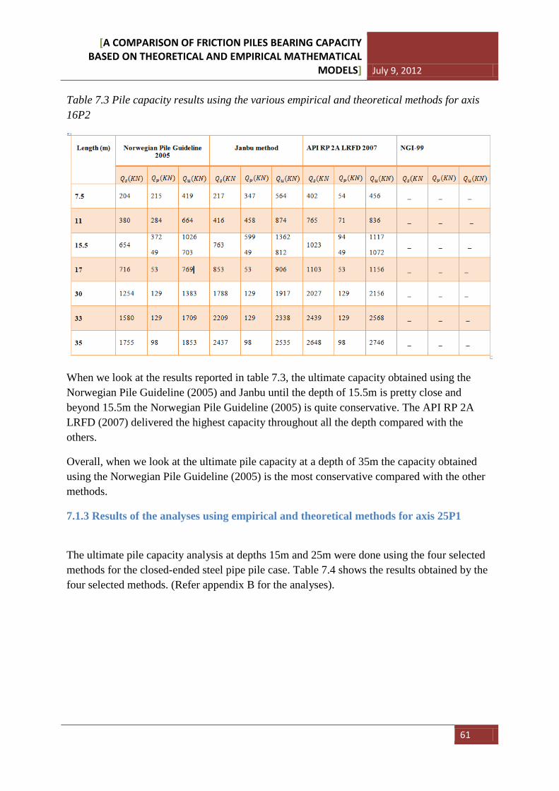
[A COMPARISON OF FRICTION PILES BEARING CAPACITY BASED ON THEORETICAL AND EMPIRICAL MATHEMATICAL
MODELS] July 9, 2012
61
Table 7.3 Pile capacity results using the various empirical and theoretical methods for axis 16P2
When we look at the results reported in table 7.3, the ultimate capacity obtained using the Norwegian Pile Guideline (2005) and Janbu until the depth of 15.5m is pretty close and beyond 15.5m the Norwegian Pile Guideline (2005) is quite conservative. The API RP 2A LRFD (2007) delivered the highest capacity throughout all the depth compared with the others.
Overall, when we look at the ultimate pile capacity at a depth of 35m the capacity obtained using the Norwegian Pile Guideline (2005) is the most conservative compared with the other methods.
7.1.3 Results of the analyses using empirical and theoretical methods for axis 25P1
The ultimate pile capacity analysis at depths 15m and 25m were done using the four selected methods for the closed-ended steel pipe pile case. Table 7.4 shows the results obtained by the four selected methods. (Refer appendix B for the analyses).
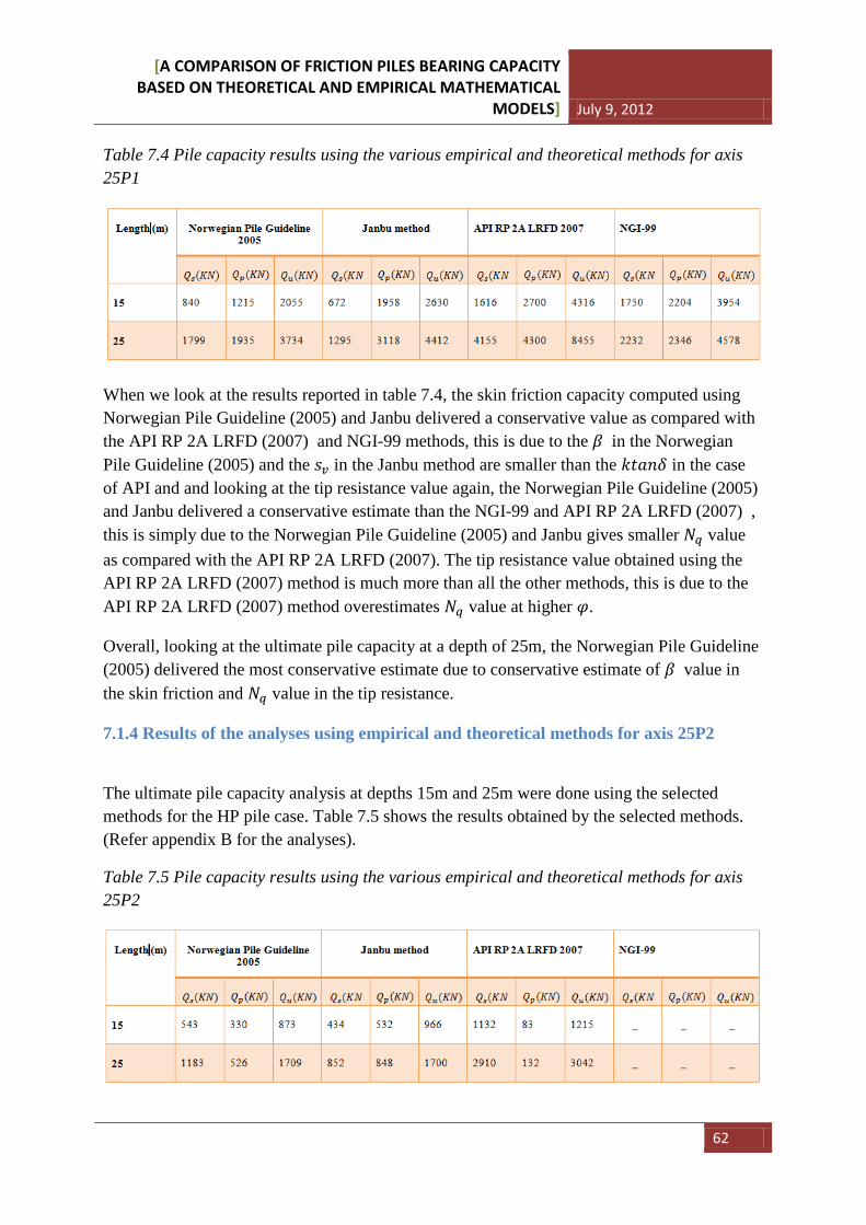
[A COMPARISON OF FRICTION PILES BEARING CAPACITY BASED ON THEORETICAL AND EMPIRICAL MATHEMATICAL
MODELS] July 9, 2012
62
Table 7.4 Pile capacity results using the various empirical and theoretical methods for axis 25P1
When we look at the results reported in table 7.4, the skin friction capacity computed using Norwegian Pile Guideline (2005) and Janbu delivered a conservative value as compared with the API RP 2A LRFD (2007) and NGI-99 methods, this is due to the 𝛽 in the Norwegian Pile Guideline (2005) and the 𝑠𝑣 in the Janbu method are smaller than the 𝑘𝑡𝑎𝑛𝛿 in the case of API and and looking at the tip resistance value again, the Norwegian Pile Guideline (2005) and Janbu delivered a conservative estimate than the NGI-99 and API RP 2A LRFD (2007) , this is simply due to the Norwegian Pile Guideline (2005) and Janbu gives smaller 𝑁𝑞 value as compared with the API RP 2A LRFD (2007). The tip resistance value obtained using the API RP 2A LRFD (2007) method is much more than all the other methods, this is due to the API RP 2A LRFD (2007) method overestimates 𝑁𝑞 value at higher 𝜑.
Overall, looking at the ultimate pile capacity at a depth of 25m, the Norwegian Pile Guideline (2005) delivered the most conservative estimate due to conservative estimate of 𝛽 value in the skin friction and 𝑁𝑞 value in the tip resistance.
7.1.4 Results of the analyses using empirical and theoretical methods for axis 25P2
The ultimate pile capacity analysis at depths 15m and 25m were done using the selected methods for the HP pile case. Table 7.5 shows the results obtained by the selected methods. (Refer appendix B for the analyses).
Table 7.5 Pile capacity results using the various empirical and theoretical methods for axis 25P2
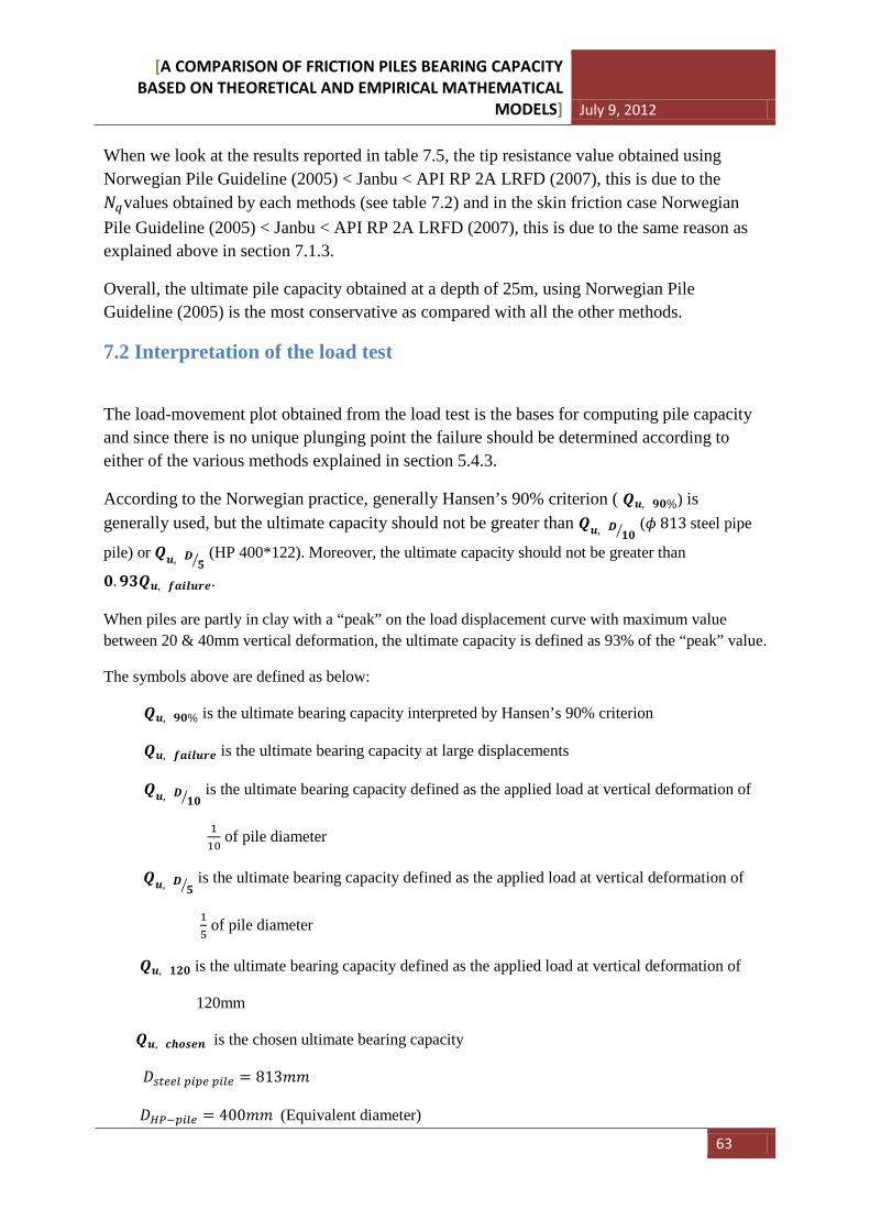
[A COMPARISON OF FRICTION PILES BEARING CAPACITY BASED ON THEORETICAL AND EMPIRICAL MATHEMATICAL
MODELS] July 9, 2012
63
When we look at the results reported in table 7.5, the tip resistance value obtained using Norwegian Pile Guideline (2005) < Janbu < API RP 2A LRFD (2007), this is due to the 𝑁𝑞values obtained by each methods (see table 7.2) and in the skin friction case Norwegian Pile Guideline (2005) < Janbu < API RP 2A LRFD (2007), this is due to the same reason as explained above in section 7.1.3.
Overall, the ultimate pile capacity obtained at a depth of 25m, using Norwegian Pile Guideline (2005) is the most conservative as compared with all the other methods.
7.2 Interpretation of the load test
The load-movement plot obtained from the load test is the bases for computing pile capacity and since there is no unique plunging point the failure should be determined according to either of the various methods explained in section 5.4.3.
According to the Norwegian practice, generally Hansen’s 90% criterion ( 𝑸𝒖, 𝟗𝟎%) is generally used, but the ultimate capacity should not be greater than 𝑸𝒖, 𝑫 𝟏𝟎� (𝜙 813 steel pipe
pile) or 𝑸𝒖, 𝑫 𝟓� (HP 400*122). Moreover, the ultimate capacity should not be greater than
𝟎.𝟗𝟑𝑸𝒖, 𝒇𝒂𝒊𝒍𝒖𝒓𝒆.
When piles are partly in clay with a “peak” on the load displacement curve with maximum value between 20 & 40mm vertical deformation, the ultimate capacity is defined as 93% of the “peak” value.
The symbols above are defined as below:
𝑸𝒖, 𝟗𝟎% is the ultimate bearing capacity interpreted by Hansen’s 90% criterion
𝑸𝒖, 𝒇𝒂𝒊𝒍𝒖𝒓𝒆 is the ultimate bearing capacity at large displacements
𝑸𝒖, 𝑫 𝟏𝟎� is the ultimate bearing capacity defined as the applied load at vertical deformation of
110
of pile diameter
𝑸𝒖, 𝑫 𝟓� is the ultimate bearing capacity defined as the applied load at vertical deformation of
15 of pile diameter
𝑸𝒖, 𝟏𝟐𝟎 is the ultimate bearing capacity defined as the applied load at vertical deformation of
120mm
𝑸𝒖, 𝒄𝒉𝒐𝒔𝒆𝒏 is the chosen ultimate bearing capacity
𝐷𝑠𝑡𝑒𝑒𝑙 𝑝𝑖𝑝𝑒 𝑝𝑖𝑙𝑒 = 813𝑚𝑚
𝐷𝐻𝑃−𝑝𝑖𝑙𝑒 = 400𝑚𝑚 (Equivalent diameter)
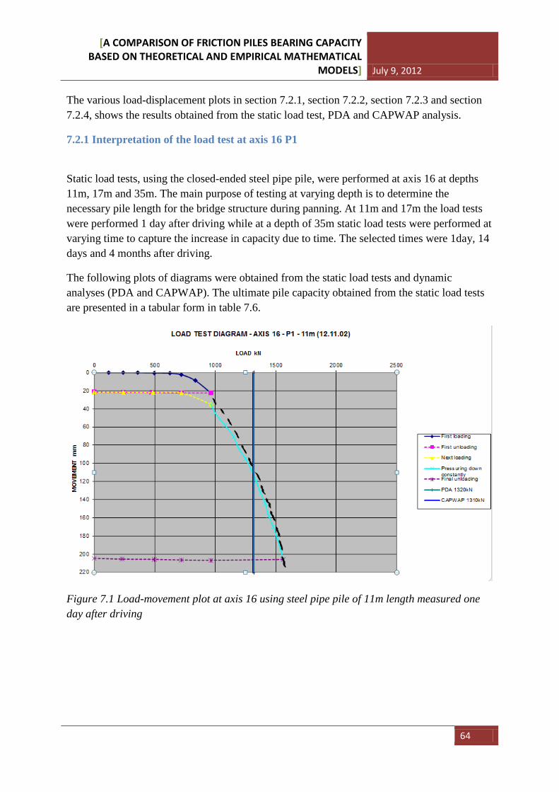
[A COMPARISON OF FRICTION PILES BEARING CAPACITY BASED ON THEORETICAL AND EMPIRICAL MATHEMATICAL
MODELS] July 9, 2012
64
The various load-displacement plots in section 7.2.1, section 7.2.2, section 7.2.3 and section 7.2.4, shows the results obtained from the static load test, PDA and CAPWAP analysis.
7.2.1 Interpretation of the load test at axis 16 P1
Static load tests, using the closed-ended steel pipe pile, were performed at axis 16 at depths 11m, 17m and 35m. The main purpose of testing at varying depth is to determine the necessary pile length for the bridge structure during panning. At 11m and 17m the load tests were performed 1 day after driving while at a depth of 35m static load tests were performed at varying time to capture the increase in capacity due to time. The selected times were 1day, 14 days and 4 months after driving.
The following plots of diagrams were obtained from the static load tests and dynamic analyses (PDA and CAPWAP). The ultimate pile capacity obtained from the static load tests are presented in a tabular form in table 7.6.
Figure 7.1 Load-movement plot at axis 16 using steel pipe pile of 11m length measured one day after driving
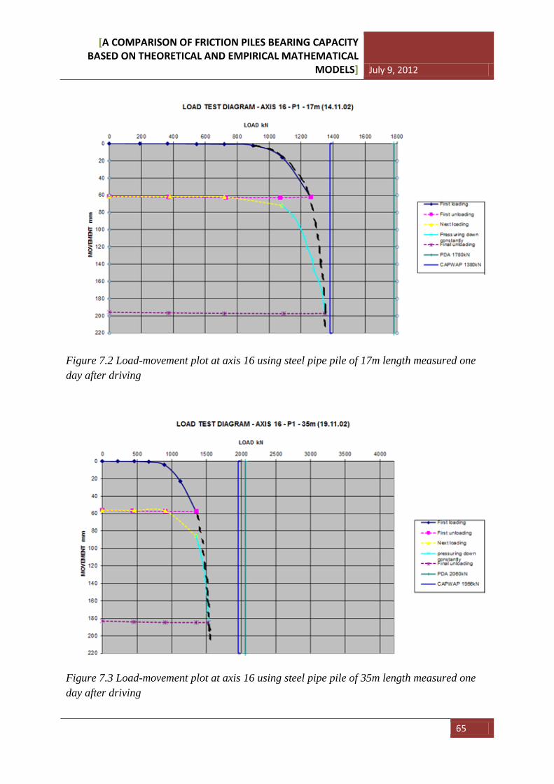
[A COMPARISON OF FRICTION PILES BEARING CAPACITY BASED ON THEORETICAL AND EMPIRICAL MATHEMATICAL
MODELS] July 9, 2012
65
Figure 7.2 Load-movement plot at axis 16 using steel pipe pile of 17m length measured one day after driving
Figure 7.3 Load-movement plot at axis 16 using steel pipe pile of 35m length measured one day after driving
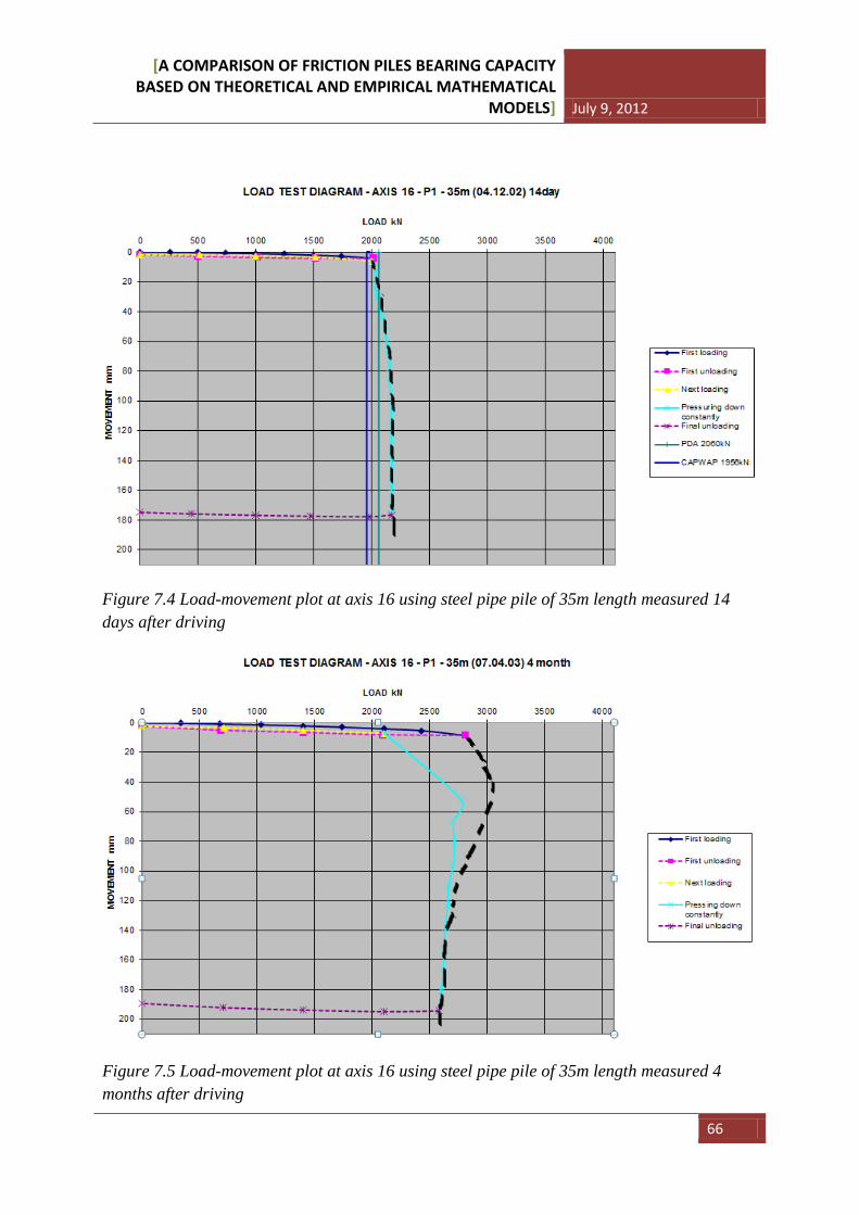
[A COMPARISON OF FRICTION PILES BEARING CAPACITY BASED ON THEORETICAL AND EMPIRICAL MATHEMATICAL
MODELS] July 9, 2012
66
Figure 7.4 Load-movement plot at axis 16 using steel pipe pile of 35m length measured 14 days after driving
Figure 7.5 Load-movement plot at axis 16 using steel pipe pile of 35m length measured 4 months after driving
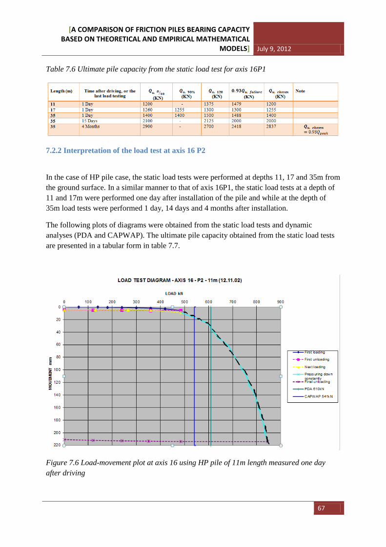
[A COMPARISON OF FRICTION PILES BEARING CAPACITY BASED ON THEORETICAL AND EMPIRICAL MATHEMATICAL
MODELS] July 9, 2012
67
Table 7.6 Ultimate pile capacity from the static load test for axis 16P1
7.2.2 Interpretation of the load test at axis 16 P2
In the case of HP pile case, the static load tests were performed at depths 11, 17 and 35m from the ground surface. In a similar manner to that of axis 16P1, the static load tests at a depth of 11 and 17m were performed one day after installation of the pile and while at the depth of 35m load tests were performed 1 day, 14 days and 4 months after installation.
The following plots of diagrams were obtained from the static load tests and dynamic analyses (PDA and CAPWAP). The ultimate pile capacity obtained from the static load tests are presented in a tabular form in table 7.7.
Figure 7.6 Load-movement plot at axis 16 using HP pile of 11m length measured one day after driving
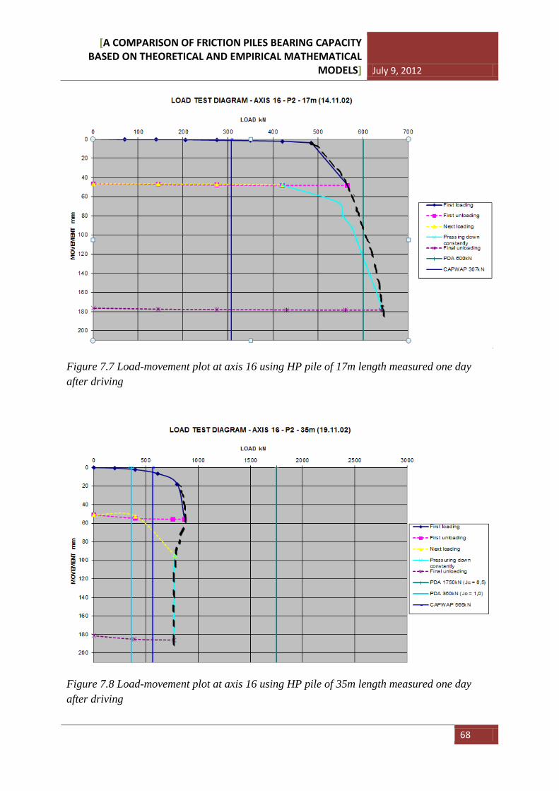
[A COMPARISON OF FRICTION PILES BEARING CAPACITY BASED ON THEORETICAL AND EMPIRICAL MATHEMATICAL
MODELS] July 9, 2012
68
Figure 7.7 Load-movement plot at axis 16 using HP pile of 17m length measured one day after driving
Figure 7.8 Load-movement plot at axis 16 using HP pile of 35m length measured one day after driving
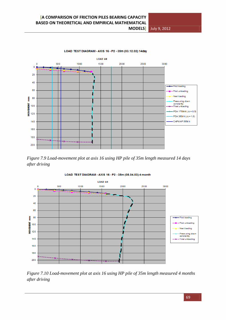
[A COMPARISON OF FRICTION PILES BEARING CAPACITY BASED ON THEORETICAL AND EMPIRICAL MATHEMATICAL
MODELS] July 9, 2012
69
Figure 7.9 Load-movement plot at axis 16 using HP pile of 35m length measured 14 days after driving
Figure 7.10 Load-movement plot at axis 16 using HP pile of 35m length measured 4 months after driving
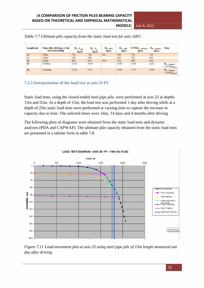
[A COMPARISON OF FRICTION PILES BEARING CAPACITY BASED ON THEORETICAL AND EMPIRICAL MATHEMATICAL
MODELS] July 9, 2012
70
Table 7.7 Ultimate pile capacity from the static load test for axis 16P2
7.2.3 Interpretation of the load test at axis 25 P1
Static load tests, using the closed-ended steel pipe pile, were performed at axis 25 at depths 15m and 25m. At a depth of 15m, the load test was performed 1 day after driving while at a depth of 25m static load tests were performed at varying time to capture the increase in capacity due to time. The selected times were 1day, 14 days and 4 months after driving.
The following plots of diagrams were obtained from the static load tests and dynamic analyses (PDA and CAPWAP). The ultimate pile capacity obtained from the static load tests are presented in a tabular form in table 7.8.
Figure 7.11 Load-movement plot at axis 25 using steel pipe pile of 15m length measured one day after driving
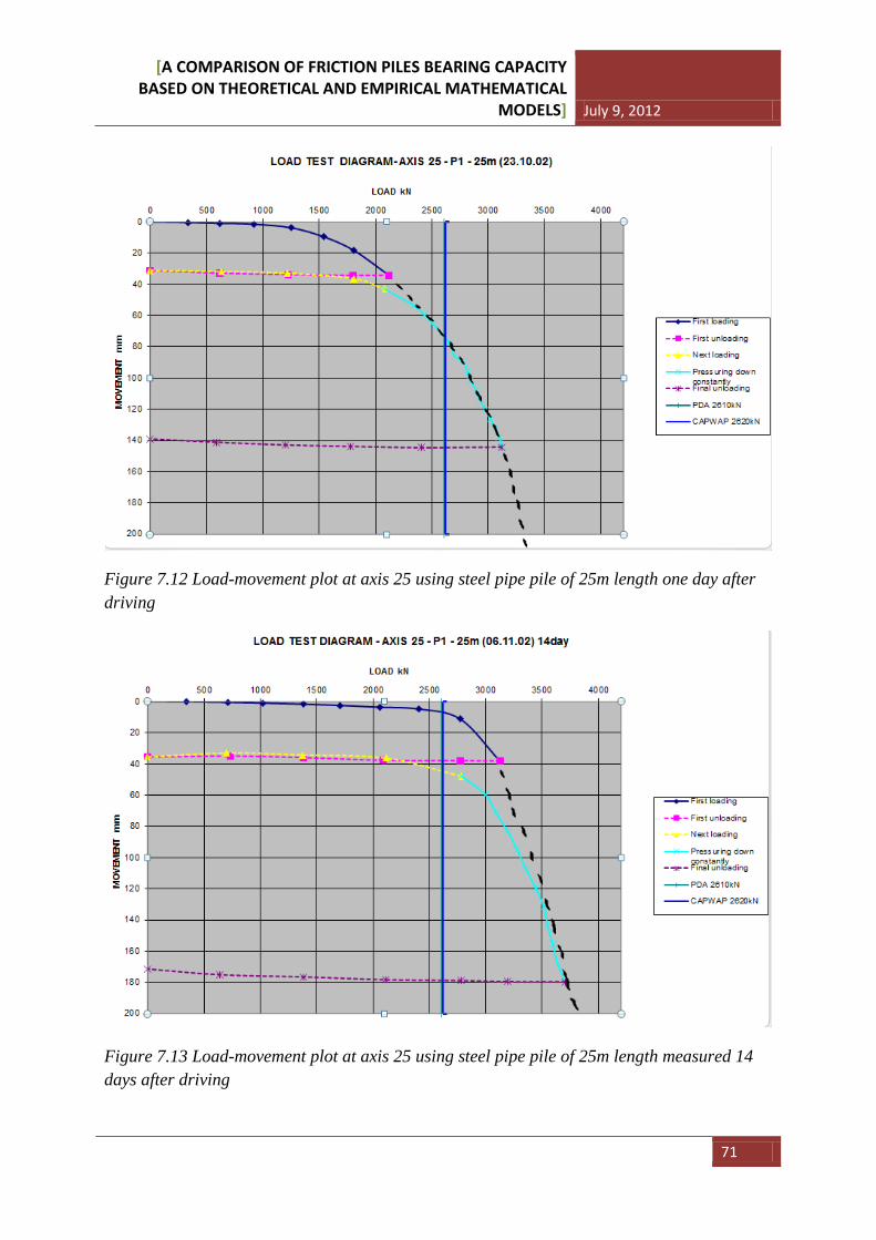
[A COMPARISON OF FRICTION PILES BEARING CAPACITY BASED ON THEORETICAL AND EMPIRICAL MATHEMATICAL
MODELS] July 9, 2012
71
Figure 7.12 Load-movement plot at axis 25 using steel pipe pile of 25m length one day after driving
Figure 7.13 Load-movement plot at axis 25 using steel pipe pile of 25m length measured 14 days after driving
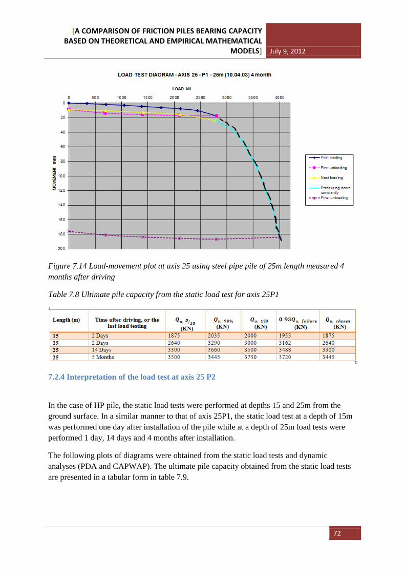
[A COMPARISON OF FRICTION PILES BEARING CAPACITY BASED ON THEORETICAL AND EMPIRICAL MATHEMATICAL
MODELS] July 9, 2012
72
Figure 7.14 Load-movement plot at axis 25 using steel pipe pile of 25m length measured 4 months after driving
Table 7.8 Ultimate pile capacity from the static load test for axis 25P1
7.2.4 Interpretation of the load test at axis 25 P2
In the case of HP pile, the static load tests were performed at depths 15 and 25m from the ground surface. In a similar manner to that of axis 25P1, the static load test at a depth of 15m was performed one day after installation of the pile while at a depth of 25m load tests were performed 1 day, 14 days and 4 months after installation.
The following plots of diagrams were obtained from the static load tests and dynamic analyses (PDA and CAPWAP). The ultimate pile capacity obtained from the static load tests are presented in a tabular form in table 7.9.
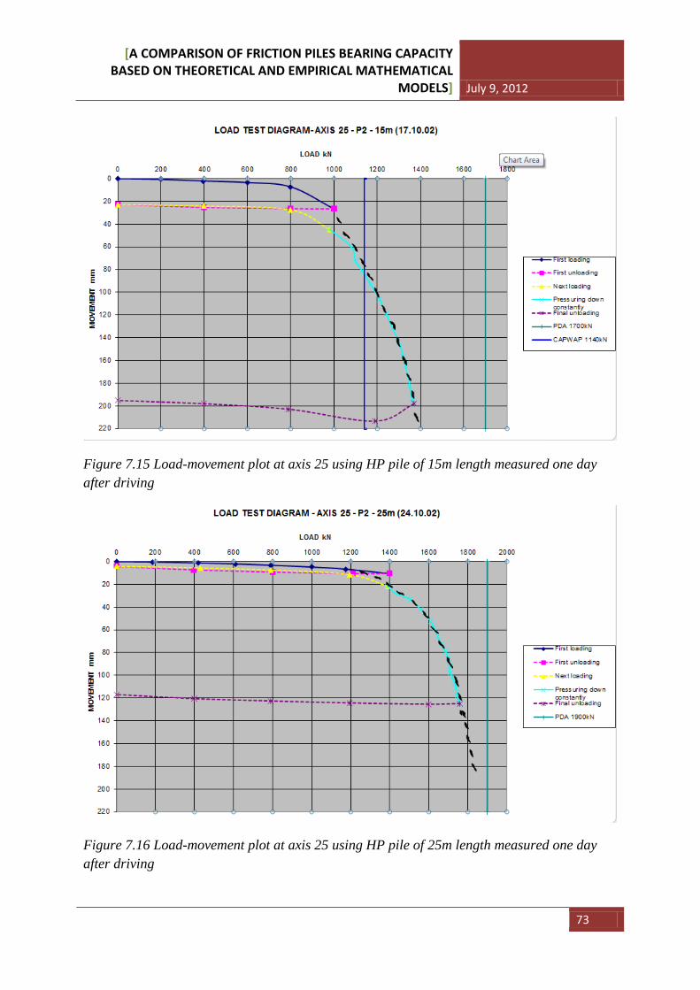
[A COMPARISON OF FRICTION PILES BEARING CAPACITY BASED ON THEORETICAL AND EMPIRICAL MATHEMATICAL
MODELS] July 9, 2012
73
Figure 7.15 Load-movement plot at axis 25 using HP pile of 15m length measured one day after driving
Figure 7.16 Load-movement plot at axis 25 using HP pile of 25m length measured one day after driving
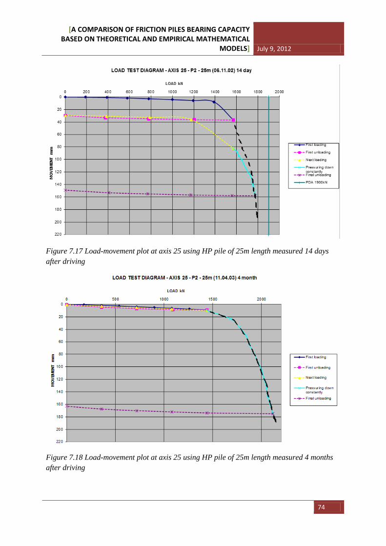
[A COMPARISON OF FRICTION PILES BEARING CAPACITY BASED ON THEORETICAL AND EMPIRICAL MATHEMATICAL
MODELS] July 9, 2012
74
Figure 7.17 Load-movement plot at axis 25 using HP pile of 25m length measured 14 days after driving
Figure 7.18 Load-movement plot at axis 25 using HP pile of 25m length measured 4 months after driving
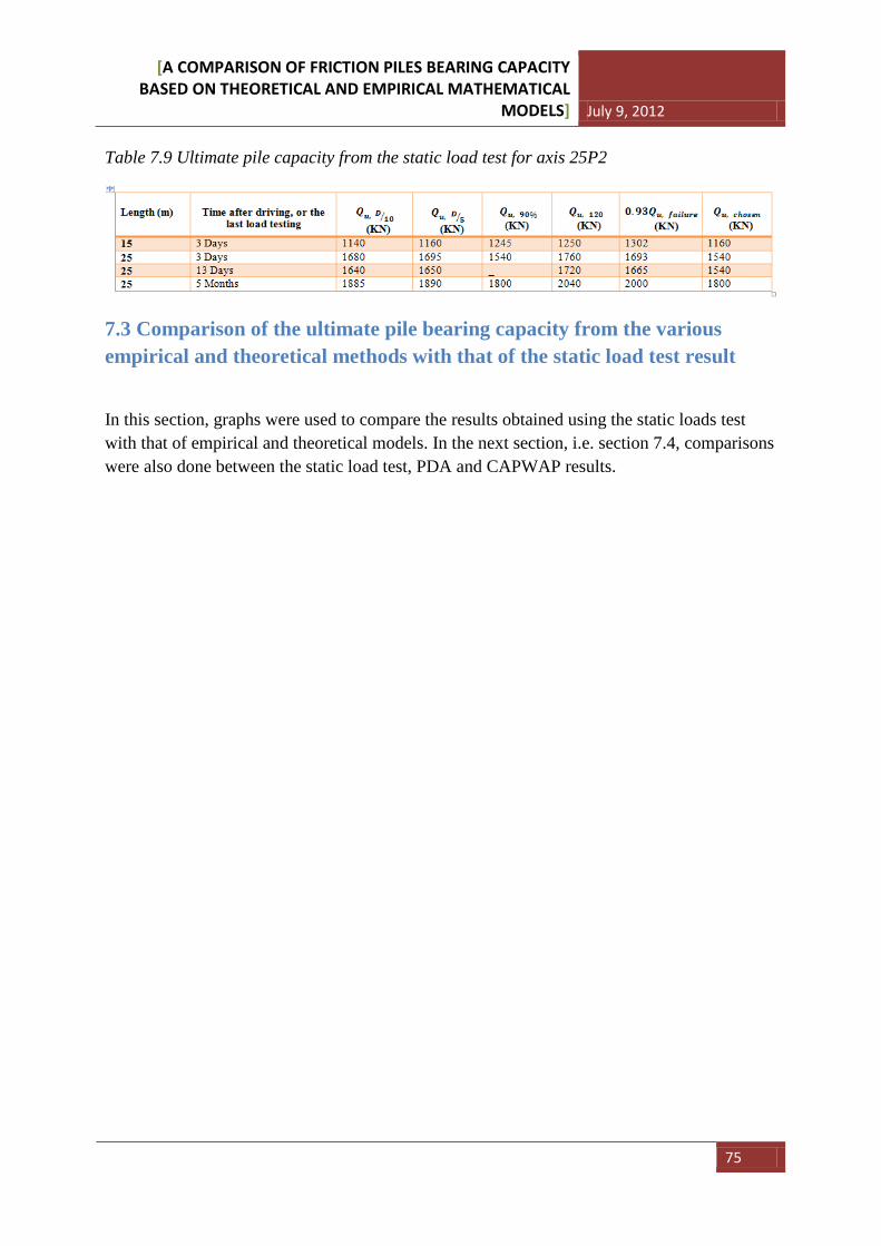
[A COMPARISON OF FRICTION PILES BEARING CAPACITY BASED ON THEORETICAL AND EMPIRICAL MATHEMATICAL
MODELS] July 9, 2012
75
Table 7.9 Ultimate pile capacity from the static load test for axis 25P2
7.3 Comparison of the ultimate pile bearing capacity from the various empirical and theoretical methods with that of the static load test result
In this section, graphs were used to compare the results obtained using the static loads test with that of empirical and theoretical models. In the next section, i.e. section 7.4, comparisons were also done between the static load test, PDA and CAPWAP results.
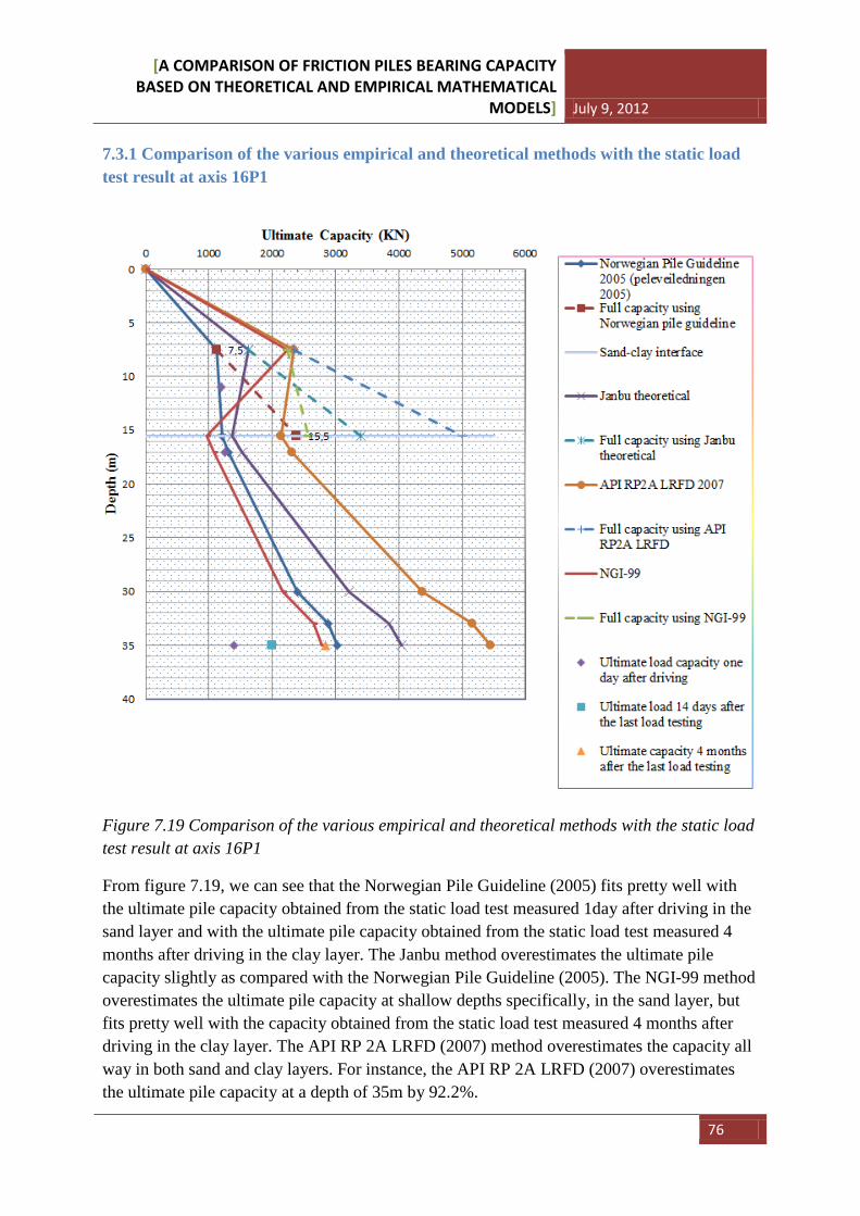
[A COMPARISON OF FRICTION PILES BEARING CAPACITY BASED ON THEORETICAL AND EMPIRICAL MATHEMATICAL
MODELS] July 9, 2012
76
7.3.1 Comparison of the various empirical and theoretical methods with the static load test result at axis 16P1
Figure 7.19 Comparison of the various empirical and theoretical methods with the static load test result at axis 16P1
From figure 7.19, we can see that the Norwegian Pile Guideline (2005) fits pretty well with the ultimate pile capacity obtained from the static load test measured 1day after driving in the sand layer and with the ultimate pile capacity obtained from the static load test measured 4 months after driving in the clay layer. The Janbu method overestimates the ultimate pile capacity slightly as compared with the Norwegian Pile Guideline (2005). The NGI-99 method overestimates the ultimate pile capacity at shallow depths specifically, in the sand layer, but fits pretty well with the capacity obtained from the static load test measured 4 months after driving in the clay layer. The API RP 2A LRFD (2007) method overestimates the capacity all way in both sand and clay layers. For instance, the API RP 2A LRFD (2007) overestimates the ultimate pile capacity at a depth of 35m by 92.2%.
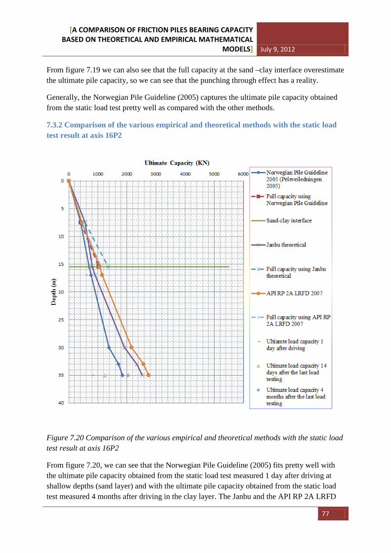
[A COMPARISON OF FRICTION PILES BEARING CAPACITY BASED ON THEORETICAL AND EMPIRICAL MATHEMATICAL
MODELS] July 9, 2012
77
From figure 7.19 we can also see that the full capacity at the sand –clay interface overestimate the ultimate pile capacity, so we can see that the punching through effect has a reality.
Generally, the Norwegian Pile Guideline (2005) captures the ultimate pile capacity obtained from the static load test pretty well as compared with the other methods.
7.3.2 Comparison of the various empirical and theoretical methods with the static load test result at axis 16P2
Figure 7.20 Comparison of the various empirical and theoretical methods with the static load test result at axis 16P2
From figure 7.20, we can see that the Norwegian Pile Guideline (2005) fits pretty well with the ultimate pile capacity obtained from the static load test measured 1 day after driving at shallow depths (sand layer) and with the ultimate pile capacity obtained from the static load test measured 4 months after driving in the clay layer. The Janbu and the API RP 2A LRFD
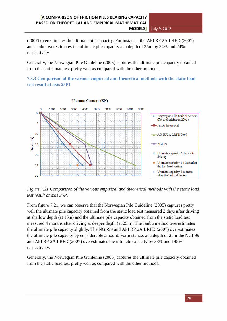
[A COMPARISON OF FRICTION PILES BEARING CAPACITY BASED ON THEORETICAL AND EMPIRICAL MATHEMATICAL
MODELS] July 9, 2012
78
(2007) overestimates the ultimate pile capacity. For instance, the API RP 2A LRFD (2007) and Janbu overestimates the ultimate pile capacity at a depth of 35m by 34% and 24% respectively.
Generally, the Norwegian Pile Guideline (2005) captures the ultimate pile capacity obtained from the static load test pretty well as compared with the other methods.
7.3.3 Comparison of the various empirical and theoretical methods with the static load test result at axis 25P1
Figure 7.21 Comparison of the various empirical and theoretical methods with the static load test result at axis 25P1
From figure 7.21, we can observe that the Norwegian Pile Guideline (2005) captures pretty well the ultimate pile capacity obtained from the static load test measured 2 days after driving at shallow depth (at 15m) and the ultimate pile capacity obtained from the static load test measured 4 months after driving at deeper depth (at 25m). The Janbu method overestimates the ultimate pile capacity slightly. The NGI-99 and API RP 2A LRFD (2007) overestimates the ultimate pile capacity by considerable amount. For instance, at a depth of 25m the NGI-99 and API RP 2A LRFD (2007) overestimates the ultimate capacity by 33% and 145% respectively.
Generally, the Norwegian Pile Guideline (2005) captures the ultimate pile capacity obtained from the static load test pretty well as compared with the other methods.
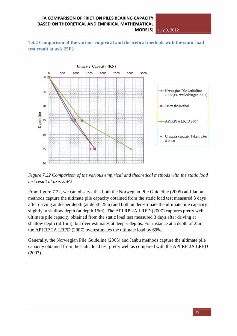
[A COMPARISON OF FRICTION PILES BEARING CAPACITY BASED ON THEORETICAL AND EMPIRICAL MATHEMATICAL
MODELS] July 9, 2012
79
7.4.4 Comparison of the various empirical and theoretical methods with the static load test result at axis 25P2
Figure 7.22 Comparison of the various empirical and theoretical methods with the static load test result at axis 25P2
From figure 7.22, we can observe that both the Norwegian Pile Guideline (2005) and Janbu methods capture the ultimate pile capacity obtained from the static load test measured 3 days after driving at deeper depth (at depth 25m) and both underestimate the ultimate pile capacity slightly at shallow depth (at depth 15m). The API RP 2A LRFD (2007) captures pretty well ultimate pile capacity obtained from the static load test measured 3 days after driving at shallow depth (at 15m), but over estimates at deeper depths. For instance at a depth of 25m the API RP 2A LRFD (2007) overestimates the ultimate load by 69%.
Generally, the Norwegian Pile Guideline (2005) and Janbu methods capture the ultimate pile capacity obtained from the static load test pretty well as compared with the API RP 2A LRFD (2007).
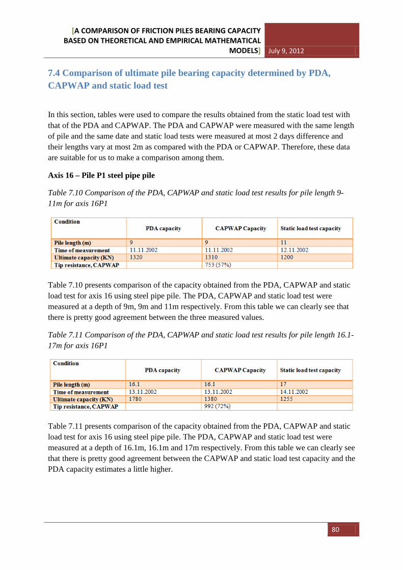
[A COMPARISON OF FRICTION PILES BEARING CAPACITY BASED ON THEORETICAL AND EMPIRICAL MATHEMATICAL
MODELS] July 9, 2012
80
7.4 Comparison of ultimate pile bearing capacity determined by PDA, CAPWAP and static load test
In this section, tables were used to compare the results obtained from the static load test with that of the PDA and CAPWAP. The PDA and CAPWAP were measured with the same length of pile and the same date and static load tests were measured at most 2 days difference and their lengths vary at most 2m as compared with the PDA or CAPWAP. Therefore, these data are suitable for us to make a comparison among them.
Axis 16 – Pile P1 steel pipe pile
Table 7.10 Comparison of the PDA, CAPWAP and static load test results for pile length 9-11m for axis 16P1
Table 7.10 presents comparison of the capacity obtained from the PDA, CAPWAP and static load test for axis 16 using steel pipe pile. The PDA, CAPWAP and static load test were measured at a depth of 9m, 9m and 11m respectively. From this table we can clearly see that there is pretty good agreement between the three measured values.
Table 7.11 Comparison of the PDA, CAPWAP and static load test results for pile length 16.1-17m for axis 16P1
Table 7.11 presents comparison of the capacity obtained from the PDA, CAPWAP and static load test for axis 16 using steel pipe pile. The PDA, CAPWAP and static load test were measured at a depth of 16.1m, 16.1m and 17m respectively. From this table we can clearly see that there is pretty good agreement between the CAPWAP and static load test capacity and the PDA capacity estimates a little higher.
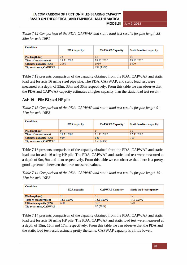
[A COMPARISON OF FRICTION PILES BEARING CAPACITY BASED ON THEORETICAL AND EMPIRICAL MATHEMATICAL
MODELS] July 9, 2012
81
Table 7.12 Comparison of the PDA, CAPWAP and static load test results for pile length 33-35m for axis 16P1
Table 7.12 presents comparison of the capacity obtained from the PDA, CAPWAP and static load test for axis 16 using steel pipe pile. The PDA, CAPWAP, and static load test were measured at a depth of 33m, 33m and 35m respectively. From this table we can observe that the PDA and CAPWAP capacity estimates a higher capacity than the static load test result.
Axis 16 – Pile P2 steel HP pile
Table 7.13 Comparison of the PDA, CAPWAP and static load test results for pile length 9-11m for axis 16P2
Table 7.13 presents comparison of the capacity obtained from the PDA, CAPWAP and static load test for axis 16 using HP pile. The PDA, CAPWAP and static load test were measured at a depth of 9m, 9m and 11m respectively. From this table we can observe that there is a pretty good agreement between the three measured values.
Table 7.14 Comparison of the PDA, CAPWAP and static load test results for pile length 15-17m for axis 16P2
Table 7.14 presents comparison of the capacity obtained from the PDA, CAPWAP and static load test for axis 16 using HP pile. The PDA, CAPWAP and static load test were measured at a depth of 15m, 15m and 17m respectively. From this table we can observe that the PDA and the static load test result estimate pretty the same. CAPWAP capacity is a little lower.
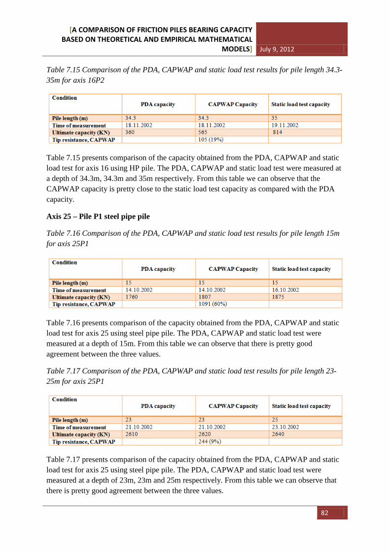
[A COMPARISON OF FRICTION PILES BEARING CAPACITY BASED ON THEORETICAL AND EMPIRICAL MATHEMATICAL
MODELS] July 9, 2012
82
Table 7.15 Comparison of the PDA, CAPWAP and static load test results for pile length 34.3-35m for axis 16P2
Table 7.15 presents comparison of the capacity obtained from the PDA, CAPWAP and static load test for axis 16 using HP pile. The PDA, CAPWAP and static load test were measured at a depth of 34.3m, 34.3m and 35m respectively. From this table we can observe that the CAPWAP capacity is pretty close to the static load test capacity as compared with the PDA capacity.
Axis 25 – Pile P1 steel pipe pile
Table 7.16 Comparison of the PDA, CAPWAP and static load test results for pile length 15m for axis 25P1
Table 7.16 presents comparison of the capacity obtained from the PDA, CAPWAP and static load test for axis 25 using steel pipe pile. The PDA, CAPWAP and static load test were measured at a depth of 15m. From this table we can observe that there is pretty good agreement between the three values.
Table 7.17 Comparison of the PDA, CAPWAP and static load test results for pile length 23-25m for axis 25P1
Table 7.17 presents comparison of the capacity obtained from the PDA, CAPWAP and static load test for axis 25 using steel pipe pile. The PDA, CAPWAP and static load test were measured at a depth of 23m, 23m and 25m respectively. From this table we can observe that there is pretty good agreement between the three values.
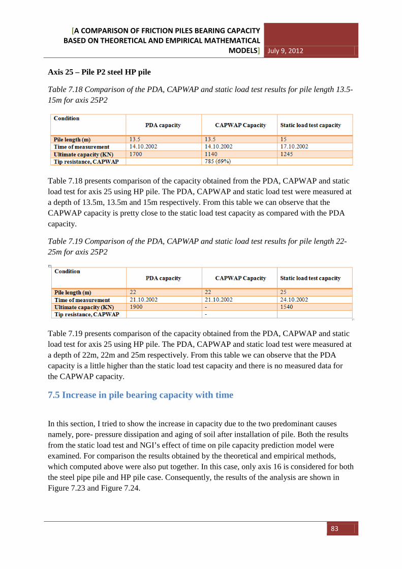
[A COMPARISON OF FRICTION PILES BEARING CAPACITY BASED ON THEORETICAL AND EMPIRICAL MATHEMATICAL
MODELS] July 9, 2012
83
Axis 25 – Pile P2 steel HP pile
Table 7.18 Comparison of the PDA, CAPWAP and static load test results for pile length 13.5-15m for axis 25P2
Table 7.18 presents comparison of the capacity obtained from the PDA, CAPWAP and static load test for axis 25 using HP pile. The PDA, CAPWAP and static load test were measured at a depth of 13.5m, 13.5m and 15m respectively. From this table we can observe that the CAPWAP capacity is pretty close to the static load test capacity as compared with the PDA capacity.
Table 7.19 Comparison of the PDA, CAPWAP and static load test results for pile length 22-25m for axis 25P2
Table 7.19 presents comparison of the capacity obtained from the PDA, CAPWAP and static load test for axis 25 using HP pile. The PDA, CAPWAP and static load test were measured at a depth of 22m, 22m and 25m respectively. From this table we can observe that the PDA capacity is a little higher than the static load test capacity and there is no measured data for the CAPWAP capacity.
7.5 Increase in pile bearing capacity with time
In this section, I tried to show the increase in capacity due to the two predominant causes namely, pore- pressure dissipation and aging of soil after installation of pile. Both the results from the static load test and NGI’s effect of time on pile capacity prediction model were examined. For comparison the results obtained by the theoretical and empirical methods, which computed above were also put together. In this case, only axis 16 is considered for both the steel pipe pile and HP pile case. Consequently, the results of the analysis are shown in Figure 7.23 and Figure 7.24.
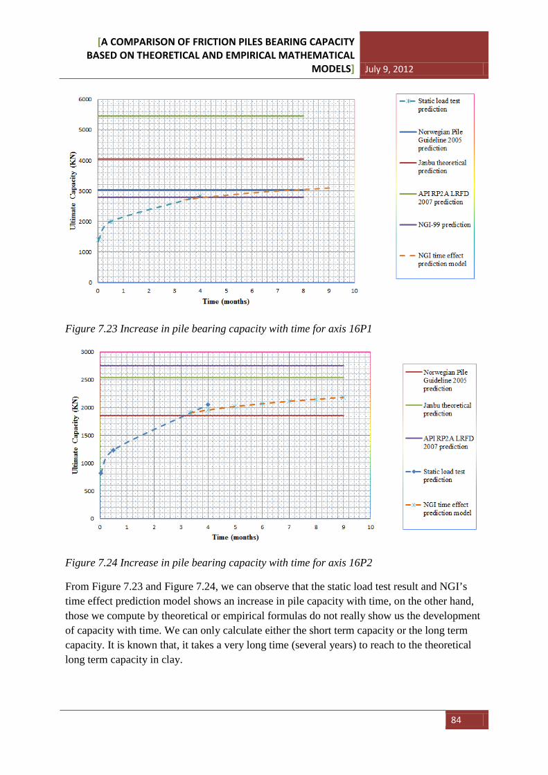
[A COMPARISON OF FRICTION PILES BEARING CAPACITY BASED ON THEORETICAL AND EMPIRICAL MATHEMATICAL
MODELS] July 9, 2012
84
Figure 7.23 Increase in pile bearing capacity with time for axis 16P1
Figure 7.24 Increase in pile bearing capacity with time for axis 16P2
From Figure 7.23 and Figure 7.24, we can observe that the static load test result and NGI’s time effect prediction model shows an increase in pile capacity with time, on the other hand, those we compute by theoretical or empirical formulas do not really show us the development of capacity with time. We can only calculate either the short term capacity or the long term capacity. It is known that, it takes a very long time (several years) to reach to the theoretical long term capacity in clay.
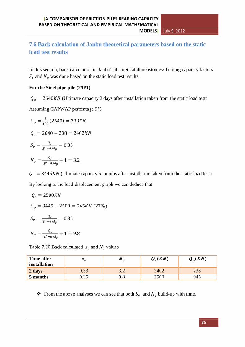
[A COMPARISON OF FRICTION PILES BEARING CAPACITY BASED ON THEORETICAL AND EMPIRICAL MATHEMATICAL
MODELS] July 9, 2012
85
7.6 Back calculation of Janbu theoretical parameters based on the static load test results
In this section, back calculation of Janbu’s theoretical dimensionless bearing capacity factors 𝑆𝑣 and 𝑁𝑞 was done based on the static load test results.
For the Steel pipe pile (25P1)
𝑄𝑢 = 2640𝐾𝑁 (Ultimate capacity 2 days after installation taken from the static load test)
Assuming CAPWAP percentage 9%
𝑄𝑝 = 9100
(2640) = 238𝐾𝑁
𝑄𝑠 = 2640 − 238 = 2402𝐾𝑁
𝑆𝑣 = 𝑄𝑠(𝑝′+𝑎)𝐴𝑝
= 0.33
𝑁𝑞 = 𝑄𝑝(𝑝′+𝑎)𝐴𝑝
+ 1 = 3.2
𝑄𝑢 = 3445𝐾𝑁 (Ultimate capacity 5 months after installation taken from the static load test)
By looking at the load-displacement graph we can deduce that
𝑄𝑠 = 2500𝐾𝑁
𝑄𝑝 = 3445 − 2500 = 945𝐾𝑁 (27%)
𝑆𝑣 = 𝑄𝑠(𝑝′+𝑎)𝐴𝑝
= 0.35
𝑁𝑞 = 𝑄𝑝(𝑝′+𝑎)𝐴𝑝
+ 1 = 9.8
Table 7.20 Back calculated 𝑠𝑣 and 𝑁𝑞 values
Time after installation
𝒔𝒗 𝑵𝒒 𝑸𝒔(𝑲𝑵) 𝑸𝒑(𝑲𝑵)
2 days 0.33 3.2 2402 238 5 months 0.35 9.8 2500 945
From the above analyses we can see that both 𝑆𝑣 and 𝑁𝑞 build-up with time.
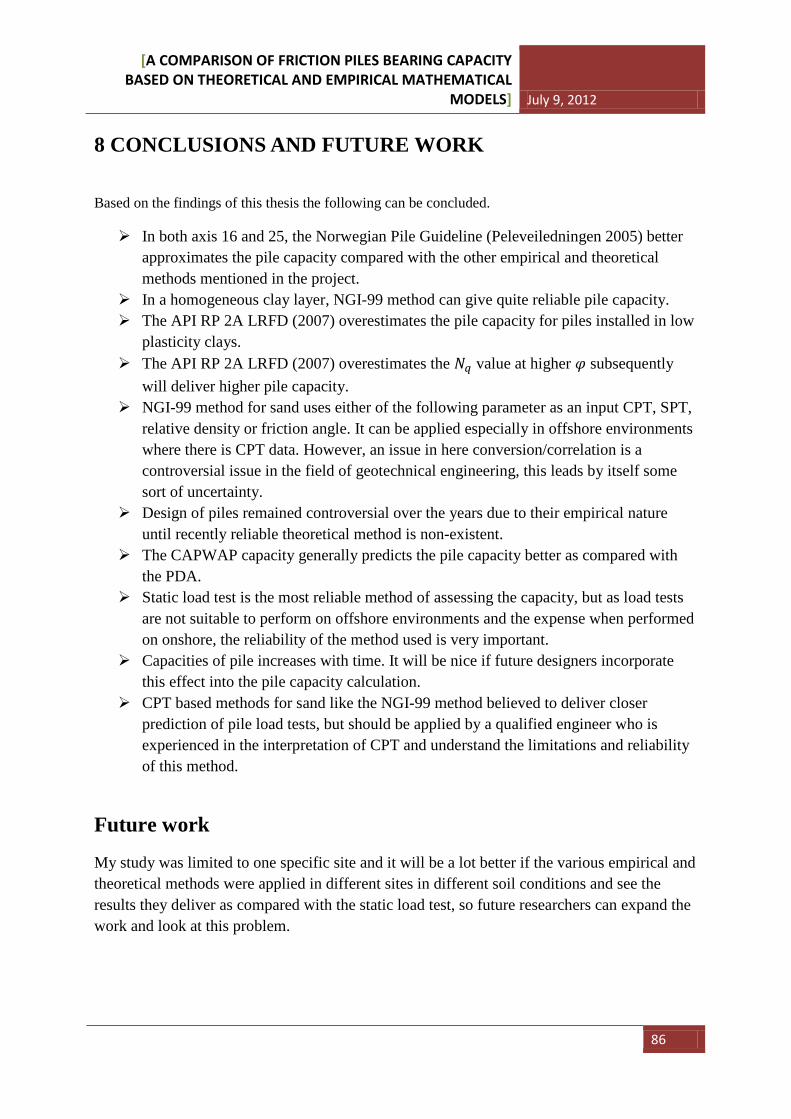
[A COMPARISON OF FRICTION PILES BEARING CAPACITY BASED ON THEORETICAL AND EMPIRICAL MATHEMATICAL
MODELS] July 9, 2012
86
8 CONCLUSIONS AND FUTURE WORK
Based on the findings of this thesis the following can be concluded.
In both axis 16 and 25, the Norwegian Pile Guideline (Peleveiledningen 2005) better approximates the pile capacity compared with the other empirical and theoretical methods mentioned in the project.
In a homogeneous clay layer, NGI-99 method can give quite reliable pile capacity. The API RP 2A LRFD (2007) overestimates the pile capacity for piles installed in low
plasticity clays. The API RP 2A LRFD (2007) overestimates the 𝑁𝑞 value at higher 𝜑 subsequently
will deliver higher pile capacity. NGI-99 method for sand uses either of the following parameter as an input CPT, SPT,
relative density or friction angle. It can be applied especially in offshore environments where there is CPT data. However, an issue in here conversion/correlation is a controversial issue in the field of geotechnical engineering, this leads by itself some sort of uncertainty.
Design of piles remained controversial over the years due to their empirical nature until recently reliable theoretical method is non-existent.
The CAPWAP capacity generally predicts the pile capacity better as compared with the PDA.
Static load test is the most reliable method of assessing the capacity, but as load tests are not suitable to perform on offshore environments and the expense when performed on onshore, the reliability of the method used is very important.
Capacities of pile increases with time. It will be nice if future designers incorporate this effect into the pile capacity calculation.
CPT based methods for sand like the NGI-99 method believed to deliver closer prediction of pile load tests, but should be applied by a qualified engineer who is experienced in the interpretation of CPT and understand the limitations and reliability of this method.
Future work
My study was limited to one specific site and it will be a lot better if the various empirical and theoretical methods were applied in different sites in different soil conditions and see the results they deliver as compared with the static load test, so future researchers can expand the work and look at this problem.
[A COMPARISON OF FRICTION PILES BEARING CAPACITY BASED ON THEORETICAL AND EMPIRICAL MATHEMATICAL
MODELS] July 9, 2012
87
REFERENCES
[1] Tomlinson, M.J. (1998). Foundation design and construction, 6th edition Pitman, London.
[2] Bowles, J.E. (1997). Foundation analysis and design, 5th edition, McGraw Hill International editions.
[3] American petroleum Institute. (1984). Recommended practice for planning, designing and constructing fixed offshore platforms. Code RP 2A, 15 Edition, Dallas, Texas.
[4] P.M. Aas. K. Karlsrud and C.J.F.Clausen. Bearing capacity of driven piles in clay, the NGI approach. Proceedings of the international symposium on Frontiers in offshore Geotechnics (IS-FOG2005), 19-21 Sept2005, Perth, WA, Australia.
[5] P.M. Aas. K. Karlsrud and C.J.F.Clausen. Bearing capacity of driven piles in sand, the NGI approach. Proceedings of the international symposium on Frontiers in offshore Geotechnics (IS-FOG2005), 19-21 Sept2005, Perth, WA, Australia.
[6] Lacasse and Nadim (1996). Model uncertainity in pile axial capacity predictions Offshore Technology Conference, Houston, May 1996, paper OCT 7996.
[7] American Petroleum Institute 1993. Recommended practice for planning, designing and constructing fixed offshore platforms –Working Stress Design, 20th edition API RP 2A-WSD, American petroleum Institute, Washington D.C., pp. 59-61. [8] Jardine R.J.& Chow F.C. 1996. New Design Methods for offshore Piles Jardine R.J. & Chow F.C. 1996. New Design Methods for Offshore Piles. Marine Technology Directorate Ltd., Publication MTD 96/103, London 1996. [9] Fugro Engineers B.V.2004. Axial Pile Capacity Design Method for Offshore Driven Piles in Sand. Report P1003 presented to the American petroleum Institute, issue 3, 5August 2004.
[10] Chow F.C., Jardine, R.J., Brucy F. & Nauroy J.F. 1998. Effects of Time on Capacity of Pipe Piles in Dense Marine Sand. ASCE, JGGE, Vol. 124, No. 3, March 1998.
[11] Lehane B.M. & Gavin K. 2004. (Discussion). Determination of bearing capacity of open-ended piles in sand. J. Geotech. & Geoenv. Engrg. ASCE, 130 (6): 656-658.
[12] Norwegian Pile Guideline 2005. (Peleveiledningen 2005)
[13] Norsk Geoteknisk Forening/NIF. Pelefundamentering i praksis. 23-25 April 2001.
[14] William Powrie Soil. Mechanics concepts and applications, 2nd edition.
[15] Shamsher Prakash Hari D. Sharma (1990). Pile foundations in engineering practice.
[16] P. Doherty. K. Gavin. The Shaft Capacity of Displacement Piles in Clay. Journal of Geotechnical and Geoenvironmental Engineering, ASCE: 389-410
[A COMPARISON OF FRICTION PILES BEARING CAPACITY BASED ON THEORETICAL AND EMPIRICAL MATHEMATICAL
MODELS] July 9, 2012
88
[17] Randolph, M.F. (2003) ‘Science and empiricism in pile foundation design’ Rankine Lecture, Geotechnique 53, No.10, pp847-875.
[18] Tomlinson, M.J. (1970). The adhesion of piles in stiff clay. Construction Industry Research and Information association Research report No. 26. London:CIRIA.
[19] Vijayvergiya, V. N. & Focht, J. A. (1972). A new way to predict the capacity of piles in clay. Proc. 4th Offshore Technology Conf. Houston 2, 865-874.
[20] Jardine, R.J., and Chow, F.C., Overy, R., and Standing, J. (2005) “ICP design methods for driven piles in sands and clays, Thomas Telford, London.
[21] White, D.J., and Lehane, B.M. (2004). “Friction fatigue on displacement piles in sand.” Geotechnique, 54(10), 645-658.
[22] Randolph, M.F., Dolwin, J., and Beck, R. 1994. Design of driven piles in sand. Geotechnique, 44(3): 427-448.
[23] Kyuho Paik and Rodrigo Salgado, M.ASCE. Determination of bearing capacity of open-ended piles in sand. Jornal of geotechnical and geoenvironmental. Vol.129, No. 1, January 2003. 46p.
[24] Kjell Karlsrud (2012). Prediction of load-displacement behavior and capacity of axially loaded piles in clay based on analyses and interpretation of pile load tests. Ph.D. Thesis. Norwegian University of Science and Technology.
[25] Fellenius, B.H., 2011. “Basics of foundation design, a text book.” Revised Electronic Edition, [www.Fellenius.net], 374p.
[26] American Petroleum institute (2000-2007). Recommended practice for planning, designing, and constructing fixed offshore platforms-working stress design. API RP 2A-WSD 21st ed. 2000, including Errata and Supplement Nos. 1-3, 2002-2007.
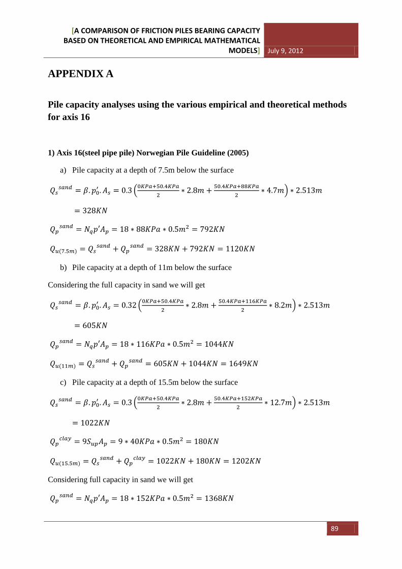
[A COMPARISON OF FRICTION PILES BEARING CAPACITY BASED ON THEORETICAL AND EMPIRICAL MATHEMATICAL
MODELS] July 9, 2012
89
APPENDIX A
Pile capacity analyses using the various empirical and theoretical methods for axis 16
1) Axis 16(steel pipe pile) Norwegian Pile Guideline (2005)
a) Pile capacity at a depth of 7.5m below the surface
𝑄𝑠𝑠𝑎𝑛𝑑 = 𝛽.𝑝0′ .𝐴𝑠 = 0.3 �0𝐾𝑃𝑎+50.4𝐾𝑃𝑎2
∗ 2.8𝑚 + 50.4𝐾𝑃𝑎+88𝐾𝑃𝑎2
∗ 4.7𝑚� ∗ 2.513𝑚
= 328𝐾𝑁
𝑄𝑝𝑠𝑎𝑛𝑑 = 𝑁𝑞𝑝′𝐴𝑝 = 18 ∗ 88𝐾𝑃𝑎 ∗ 0.5𝑚2 = 792𝐾𝑁
𝑄𝑢(7.5𝑚) = 𝑄𝑠𝑠𝑎𝑛𝑑 + 𝑄𝑝𝑠𝑎𝑛𝑑 = 328𝐾𝑁 + 792𝐾𝑁 = 1120𝐾𝑁
b) Pile capacity at a depth of 11m below the surface
Considering the full capacity in sand we will get
𝑄𝑠𝑠𝑎𝑛𝑑 = 𝛽.𝑝0′ .𝐴𝑠 = 0.32 �0𝐾𝑃𝑎+50.4𝐾𝑃𝑎2
∗ 2.8𝑚 + 50.4𝐾𝑃𝑎+116𝐾𝑃𝑎2
∗ 8.2𝑚� ∗ 2.513𝑚
= 605𝐾𝑁
𝑄𝑝𝑠𝑎𝑛𝑑 = 𝑁𝑞𝑝′𝐴𝑝 = 18 ∗ 116𝐾𝑃𝑎 ∗ 0.5𝑚2 = 1044𝐾𝑁
𝑄𝑢(11𝑚) = 𝑄𝑠𝑠𝑎𝑛𝑑 + 𝑄𝑝𝑠𝑎𝑛𝑑 = 605𝐾𝑁 + 1044𝐾𝑁 = 1649𝐾𝑁
c) Pile capacity at a depth of 15.5m below the surface
𝑄𝑠𝑠𝑎𝑛𝑑 = 𝛽.𝑝0′ .𝐴𝑠 = 0.3 �0𝐾𝑃𝑎+50.4𝐾𝑃𝑎2
∗ 2.8𝑚 + 50.4𝐾𝑃𝑎+152𝐾𝑃𝑎2
∗ 12.7𝑚� ∗ 2.513𝑚
= 1022𝐾𝑁
𝑄𝑝𝑐𝑙𝑎𝑦 = 9𝑆𝑢𝑝𝐴𝑝 = 9 ∗ 40𝐾𝑃𝑎 ∗ 0.5𝑚2 = 180𝐾𝑁
𝑄𝑢(15.5𝑚) = 𝑄𝑠𝑠𝑎𝑛𝑑 + 𝑄𝑝𝑐𝑙𝑎𝑦 = 1022𝐾𝑁 + 180𝐾𝑁 = 1202𝐾𝑁
Considering full capacity in sand we will get
𝑄𝑝𝑠𝑎𝑛𝑑 = 𝑁𝑞𝑝′𝐴𝑝 = 18 ∗ 152𝐾𝑃𝑎 ∗ 0.5𝑚2 = 1368𝐾𝑁
[A COMPARISON OF FRICTION PILES BEARING CAPACITY BASED ON THEORETICAL AND EMPIRICAL MATHEMATICAL
MODELS] July 9, 2012
90
𝑄𝑢(15.5𝑚) = 𝑄𝑠𝑠𝑎𝑛𝑑 + 𝑄𝑝𝑠𝑎𝑛𝑑 = 1022𝐾𝑁 + 1368𝐾𝑁 = 2390𝐾𝑁
d) Pile capacity at a depth of 17m below the surface
𝑄𝑠𝑠𝑎𝑛𝑑+𝑐𝑙𝑎𝑦 = 1022𝐾𝑁 + (𝛼𝑆𝑢𝐴𝑠) = 1022𝐾𝑁 + (0.62 ∗ 41𝐾𝑃𝑎 ∗ 2.513𝑚 ∗ 1.5𝑚)
= 1118𝐾𝑁
𝑄𝑝𝑐𝑙𝑎𝑦 = 9𝑆𝑢𝑝𝐴𝑝 = 9 ∗ 43𝐾𝑃𝑎 ∗ 0.5𝑚2 = 194𝐾𝑁
𝑄𝑢(17𝑚) = 𝑄𝑠𝑠𝑎𝑛𝑑+𝑐𝑙𝑎𝑦 + 𝑄𝑝𝑐𝑙𝑎𝑦 = 1118𝐾𝑁 + 194𝐾𝑁 = 1312𝐾𝑁
e) Pile capacity at a depth of 30m below the surface
𝑄𝑠𝑠𝑎𝑛𝑑+𝑐𝑙𝑎𝑦 = 1022𝐾𝑁 + (𝛼𝑆𝑢𝐴𝑠) = 1022𝐾𝑁 + (0.62 ∗ 40𝐾𝑃𝑎 ∗ 2.513𝑚 ∗ 14.5𝑚)
= 1926𝐾𝑁
𝑄𝑝𝑐𝑙𝑎𝑦 = 9𝑆𝑢𝑝𝐴𝑝 = 9 ∗ 105𝐾𝑃𝑎 ∗ 0.5𝑚2 = 473𝐾𝑁
𝑄𝑢(30𝑚) = 𝑄𝑠𝑠𝑎𝑛𝑑+𝑐𝑙𝑎𝑦 + 𝑄𝑝𝑐𝑙𝑎𝑦 = 1926𝐾𝑁 + 473𝐾𝑁 = 2399𝐾𝑁
f) Pile capacity at a depth of 33m below the surface
𝑄𝑠𝑠𝑎𝑛𝑑+𝑐𝑙𝑎𝑦 = 1926𝐾𝑁 + (𝛼𝑆𝑢𝐴𝑠) = 1926𝐾𝑁 + (0.62 ∗ 105𝐾𝑃𝑎 ∗ 2.513𝑚 ∗ 3𝑚)
= 2417𝐾𝑁
𝑄𝑝𝑐𝑙𝑎𝑦 = 9𝑆𝑢𝑝𝐴𝑝 = 9 ∗ 105𝐾𝑃𝑎 ∗ 0.5𝑚2 = 473𝐾𝑁
𝑄𝑢(33𝑚) = 𝑄𝑠𝑠𝑎𝑛𝑑+𝑐𝑙𝑎𝑦 + 𝑄𝑝𝑐𝑙𝑎𝑦 = 2417𝐾𝑁 + 473𝐾𝑁 = 2890𝐾𝑁
g) Pile capacity at a depth of 35m below the surface
𝑄𝑠𝑠𝑎𝑛𝑑+𝑐𝑙𝑎𝑦 = 2417𝐾𝑁 + (𝛼𝑆𝑢𝐴𝑠) = 2417𝐾𝑁 + (0.62 ∗ 80𝐾𝑃𝑎 ∗ 2.513𝑚 ∗ 2𝑚)
= 2666𝐾𝑁
𝑄𝑝𝑐𝑙𝑎𝑦 = 9𝑆𝑢𝑝𝐴𝑝 = 9 ∗ 80𝐾𝑃𝑎 ∗ 0.5𝑚2 = 360𝐾𝑁
𝑄𝑢(33𝑚) = 𝑄𝑠𝑠𝑎𝑛𝑑+𝑐𝑙𝑎𝑦 + 𝑄𝑝𝑐𝑙𝑎𝑦 = 2666𝐾𝑁 + 360𝐾𝑁 = 3026𝐾𝑁
2) Axis 16 (HP pile) Norwegian Pile Guideline (2005)
a) Pile capacity at a depth of 7.5m below the surface
𝑄𝑠𝑠𝑎𝑛𝑑 = 328𝐾𝑁 ∗ 1.476𝑚2.513𝑚
∗ 1.06 = 204𝐾𝑁
[A COMPARISON OF FRICTION PILES BEARING CAPACITY BASED ON THEORETICAL AND EMPIRICAL MATHEMATICAL
MODELS] July 9, 2012
91
𝑄𝑝𝑠𝑎𝑛𝑑 = 792𝐾𝑁 ∗ 0.136𝑚2
0.5𝑚2 = 215𝐾𝑁
𝑄𝑢(7.5𝑚) = 𝑄𝑠𝑠𝑎𝑛𝑑 + 𝑄𝑝𝑠𝑎𝑛𝑑 = 204𝐾𝑁 + 215𝐾𝑁 = 419𝐾𝑁
b) Pile capacity at a depth of 11m below the surface
Considering the full capacity in sand we will get:
𝑄𝑠𝑠𝑎𝑛𝑑 = 605𝐾𝑁 ∗ 1.476𝑚2.513𝑚
∗ 1.07 = 380𝐾𝑁
𝑄𝑝𝑠𝑎𝑛𝑑 = 1044𝐾𝑁 ∗ 0.136𝑚2
0.5𝑚2 = 284𝐾𝑁
𝑄𝑢(11𝑚) = 𝑄𝑠𝑠𝑎𝑛𝑑 + 𝑄𝑝𝑠𝑎𝑛𝑑 = 380𝐾𝑁 + 284𝐾𝑁 = 664𝐾𝑁
c) Pile capacity at a depth of 15.5m below the surface
𝑄𝑠𝑠𝑎𝑛𝑑 = 1022𝐾𝑁 ∗ 1.476𝑚2.513𝑚
∗ 1.09 = 654𝐾𝑁
𝑄𝑝𝑐𝑙𝑎𝑦 = 180𝐾𝑁 ∗ 0.136𝑚2
0.5𝑚2 = 49𝐾𝑁
𝑄𝑢(15.5𝑚) = 𝑄𝑠𝑠𝑎𝑛𝑑 + 𝑄𝑝𝑐𝑙𝑎𝑦 = 654𝐾𝑁 + 49𝐾𝑁 = 703𝐾𝑁
Considering the full capacity in sand we will get
𝑄𝑝𝑠𝑎𝑛𝑑 = 1368𝐾𝑁 ∗ 0.136𝑚2
0.5𝑚2 = 372𝐾𝑁
𝑄𝑢(15.5𝑚) = 𝑄𝑠𝑠𝑎𝑛𝑑 + 𝑄𝑝𝑠𝑎𝑛𝑑 = 654𝐾𝑁 + 372𝐾𝑁 = 1026𝐾𝑁
d) Pile capacity at a depth of 17m below the surface
𝑄𝑠𝑠𝑎𝑛𝑑 = 654𝐾𝑁
𝑄𝑠𝑐𝑙𝑎𝑦 = 96𝐾𝑁 ∗ 1.476𝑚2.513𝑚
∗ 1.1 = 62𝐾𝑁
𝑄𝑝𝑐𝑙𝑎𝑦 = 194𝐾𝑁 ∗ 0.136𝑚2
0.5𝑚2 = 53𝐾𝑁
𝑄𝑢(17𝑚) = 𝑄𝑠𝑠𝑎𝑛𝑑 + 𝑄𝑠𝑐𝑙𝑎𝑦 + 𝑄𝑝𝑐𝑙𝑎𝑦 = 654𝐾𝑁 + 62𝐾𝑁 + 53𝐾𝑁 = 769𝐾𝑁
e) Pile capacity at a depth of 30m below the surface
𝑄𝑠𝑠𝑎𝑛𝑑 = 654𝐾𝑁
𝑄𝑠𝑐𝑙𝑎𝑦 = 904𝐾𝑁 ∗ 1.476𝑚2.513𝑚
∗ 1.13 = 600𝐾𝑁
[A COMPARISON OF FRICTION PILES BEARING CAPACITY BASED ON THEORETICAL AND EMPIRICAL MATHEMATICAL
MODELS] July 9, 2012
92
𝑄𝑝𝑐𝑙𝑎𝑦 = 473𝐾𝑁 ∗ 0.136𝑚2
0.5𝑚2 = 129𝐾𝑁
𝑄𝑢(30𝑚) = 𝑄𝑠𝑠𝑎𝑛𝑑 + 𝑄𝑠𝑐𝑙𝑎𝑦 + 𝑄𝑝𝑐𝑙𝑎𝑦 = 654𝐾𝑁 + 600𝐾𝑁 + 129𝐾𝑁 = 1383𝐾𝑁
f) Pile capacity at a depth of 33m below the surface
𝑄𝑠𝑠𝑎𝑛𝑑 = 654𝐾𝑁
𝑄𝑠𝑐𝑙𝑎𝑦 = (904𝐾𝑁 + 491𝐾𝑁) ∗ 1.476𝑚2.513𝑚
∗ 1.13 = 926𝐾𝑁
𝑄𝑝𝑐𝑙𝑎𝑦 = 473𝐾𝑁 ∗ 0.136𝑚2
0.5𝑚2 = 129𝐾𝑁
𝑄𝑢(33𝑚) = 𝑄𝑠𝑠𝑎𝑛𝑑 + 𝑄𝑠𝑐𝑙𝑎𝑦 + 𝑄𝑝𝑐𝑙𝑎𝑦 = 654𝐾𝑁 + 926𝐾𝑁 + 129𝐾𝑁 = 1709𝐾𝑁
g) Pile capacity at a depth of 35m below the surface
𝑄𝑠𝑠𝑎𝑛𝑑 = 654𝐾𝑁
𝑄𝑠𝑐𝑙𝑎𝑦 = (904𝐾𝑁 + 491𝐾𝑁 + 249𝐾𝑁) ∗ 1.476𝑚2.513𝑚
∗ 1.14 = 1101𝐾𝑁
𝑄𝑝𝑐𝑙𝑎𝑦 = 360𝐾𝑁 ∗ 0.136𝑚2
0.5𝑚2 = 98𝐾𝑁
𝑄𝑢(35𝑚) = 𝑄𝑠𝑠𝑎𝑛𝑑 + 𝑄𝑠𝑐𝑙𝑎𝑦 + 𝑄𝑝𝑐𝑙𝑎𝑦 = 654𝐾𝑁 + 1101𝐾𝑁 + 98𝐾𝑁 = 1853𝐾𝑁
3) Axis 16 (steel pipe pile) Janbu theoretical
a) Pile capacity at a depth of 7.5m below the surface
From chart;
𝑡𝑎𝑛𝜑 = 0.7, 𝑟 = 0.9 → 𝑆𝑣 = 0.35
𝑡𝑎𝑛𝜑 = 0.7, 𝛽 = 0 → 𝑁𝑞 = 30
𝑄𝑠𝑠𝑎𝑛𝑑 = 𝑆𝑣(𝑝′ + 𝑎)𝐴𝑠 = 0.35 �0𝐾𝑃𝑎+50.4𝐾𝑃𝑎2
∗ 2.8𝑚 + 50.4𝐾𝑃𝑎+88𝐾𝑃𝑎2
∗ 4.7𝑚� ∗ 2.513
= 348𝐾𝑁
𝑄𝑝𝑠𝑎𝑛𝑑 = �𝑁𝑞 − 1�(𝑝′ + 𝑎)𝐴𝑝 = (30 − 1) ∗ 88𝐾𝑃𝑎 ∗ 0.5𝑚2 = 1276𝐾𝑁
𝑄𝑢(7.5𝑚) = 𝑄𝑠𝑠𝑎𝑛𝑑 + 𝑄𝑝𝑠𝑎𝑛𝑑 = 348𝐾𝑁 + 1276𝐾𝑁 = 1624𝐾𝑁
b) Pile capacity at a depth of 11m below the surface
Considering the full capacity in sand we will get:
[A COMPARISON OF FRICTION PILES BEARING CAPACITY BASED ON THEORETICAL AND EMPIRICAL MATHEMATICAL
MODELS] July 9, 2012
93
From chart;
𝑡𝑎𝑛𝜑 = 0.7, 𝑟 = 0.9 → 𝑆𝑣 = 0.35
𝑡𝑎𝑛𝜑 = 0.7, 𝛽 = 0 → 𝑁𝑞 = 30
𝑄𝑠𝑠𝑎𝑛𝑑 = 𝑆𝑣(𝑝′ + 𝑎)𝐴𝑠 = 0.35 �0𝐾𝑃𝑎+50.4𝐾𝑃𝑎2
∗ 2.8𝑚 + 50.4𝐾𝑃𝑎+116𝐾𝑃𝑎2
∗ 8.2𝑚� ∗ 2.513
= 662𝐾𝑁
𝑄𝑝𝑠𝑎𝑛𝑑 = �𝑁𝑞 − 1�(𝑝′ + 𝑎)𝐴𝑝 = (30 − 1) ∗ 116𝐾𝑃𝑎 ∗ 0.5𝑚2 = 1682𝐾𝑁
𝑄𝑢(11𝑚) = 𝑄𝑠𝑠𝑎𝑛𝑑 + 𝑄𝑝𝑠𝑎𝑛𝑑 = 662𝐾𝑁 + 1682𝐾𝑁 = 2344𝐾𝑁
c) Pile capacity at a depth of 15.5m below the surface
𝑡𝑎𝑛𝜑 = 0.7, 𝑟 = 0.9 → 𝑆𝑣 = 0.35
𝑡𝑎𝑛𝜑 = 0.7, 𝛽 = 0 → 𝑁𝑞 = 30
𝑄𝑠𝑠𝑎𝑛𝑑 = 𝑆𝑣(𝑝′ + 𝑎)𝐴𝑠 = 0.35 �0𝐾𝑃𝑎+50.4𝐾𝑃𝑎2
∗ 2.8𝑚 + 50.4𝐾𝑃𝑎+152𝐾𝑃𝑎2
∗ 12.7𝑚� ∗ 2.513
= 1192𝐾𝑁
𝑄𝑝𝑐𝑙𝑎𝑦 = 9𝑆𝑢𝑝𝐴𝑝 = 9 ∗ 40𝐾𝑃𝑎 ∗ 0.5𝑚2 = 180𝐾𝑁
𝑄𝑢(15.5𝑚) = 𝑄𝑠𝑠𝑎𝑛𝑑 + 𝑄𝑝𝑐𝑙𝑎𝑦 = 1192𝐾𝑁 + 180𝐾𝑁 = 1372𝐾𝑁
Considering the full capacity in sand we will get:
𝑄𝑝𝑠𝑎𝑛𝑑 = �𝑁𝑞 − 1�(𝑝′ + 𝑎)𝐴𝑝 = (30 − 1) ∗ 152𝐾𝑃𝑎 ∗ 0.5𝑚2 = 2204𝐾𝑁
𝑄𝑢(15.5𝑚) = 𝑄𝑠𝑠𝑎𝑛𝑑 + 𝑄𝑝𝑠𝑎𝑛𝑑 = 1192𝐾𝑁 + 2204𝐾𝑁 = 3396𝐾𝑁
d) Pile capacity at a depth of 17m below the surface
𝑄𝑠𝑠𝑎𝑛𝑑+𝑐𝑙𝑎𝑦 = 1192𝐾𝑁 + (𝑟𝑆𝑢𝐴𝑠) = 1192𝐾𝑁 + (0.9 ∗ 41𝐾𝑃𝑎 ∗ 2.513𝑚 ∗ 1.5𝑚)
= 1331𝐾𝑁
𝑄𝑝𝑐𝑙𝑎𝑦 = 9𝑆𝑢𝑝𝐴𝑝 = 9 ∗ 43𝐾𝑃𝑎 ∗ 0.5𝑚2 = 194𝐾𝑁
𝑄𝑢(17𝑚) = 𝑄𝑠𝑠𝑎𝑛𝑑+𝑐𝑙𝑎𝑦 + 𝑄𝑝𝑐𝑙𝑎𝑦 = 1331𝐾𝑁 + 194𝐾𝑁 = 1525𝐾𝑁
e) Pile capacity at a depth of 30m below the surface
𝑄𝑠𝑠𝑎𝑛𝑑+𝑐𝑙𝑎𝑦 = 1192𝐾𝑁 + (𝑟𝑆𝑢𝐴𝑠) = 1192𝐾𝑁 + (0.8 ∗ 53𝐾𝑃𝑎 ∗ 2.513𝑚 ∗ 14.5𝑚)
[A COMPARISON OF FRICTION PILES BEARING CAPACITY BASED ON THEORETICAL AND EMPIRICAL MATHEMATICAL
MODELS] July 9, 2012
94
= 2737𝐾𝑁
𝑄𝑝𝑐𝑙𝑎𝑦 = 9𝑆𝑢𝑝𝐴𝑝 = 9 ∗ 105𝐾𝑃𝑎 ∗ 0.5𝑚2 = 473𝐾𝑁
𝑄𝑢(30𝑚) = 𝑄𝑠𝑠𝑎𝑛𝑑+𝑐𝑙𝑎𝑦 + 𝑄𝑝𝑐𝑙𝑎𝑦 = 2737𝐾𝑁 + 473𝐾𝑁 = 3210𝐾𝑁
f) Pile capacity at a depth of 33m below the surface
𝑄𝑠𝑠𝑎𝑛𝑑+𝑐𝑙𝑎𝑦 = 2737𝐾𝑁 + (𝑟𝑆𝑢𝐴𝑠) = 2737𝐾𝑁 + (0.8 ∗ 105𝐾𝑃𝑎 ∗ 2.513𝑚 ∗ 3𝑚)
= 3370𝐾𝑁
𝑄𝑝𝑐𝑙𝑎𝑦 = 9𝑆𝑢𝑝𝐴𝑝 = 9 ∗ 105𝐾𝑃𝑎 ∗ 0.5𝑚2 = 473𝐾𝑁
𝑄𝑢(33𝑚) = 𝑄𝑠𝑠𝑎𝑛𝑑+𝑐𝑙𝑎𝑦 + 𝑄𝑝𝑐𝑙𝑎𝑦 = 3370𝐾𝑁 + 473𝐾𝑁 = 3843𝐾𝑁
g) Pile capacity at a depth of 35m below the surface
𝑄𝑠𝑠𝑎𝑛𝑑+𝑐𝑙𝑎𝑦 = 3370𝐾𝑁 + (𝑟𝑆𝑢𝐴𝑠) = 3370𝐾𝑁 + (0.8 ∗ 80𝐾𝑃𝑎 ∗ 2.513𝑚 ∗ 2𝑚)
= 3692𝐾𝑁
𝑄𝑝𝑐𝑙𝑎𝑦 = 9𝑆𝑢𝑝𝐴𝑝 = 9 ∗ 80𝐾𝑃𝑎 ∗ 0.5𝑚2 = 360𝐾𝑁
𝑄𝑢(35𝑚) = 𝑄𝑠𝑠𝑎𝑛𝑑+𝑐𝑙𝑎𝑦 + 𝑄𝑝𝑐𝑙𝑎𝑦 = 3692𝐾𝑁 + 360𝐾𝑁 = 4052𝐾𝑁
4) Axis 16 (HP pile) Janbu theoretical
a) Pile capacity at a depth of 7.5m below the surface
𝑄𝑠𝑠𝑎𝑛𝑑 = 348𝐾𝑁 ∗ 1.476𝑚2.513𝑚
∗ 1.06 = 217𝐾𝑁
𝑄𝑝𝑠𝑎𝑛𝑑 = 1276𝐾𝑁 ∗ 0.136𝑚2
0.5𝑚2 = 347𝐾𝑁
𝑄𝑢(7.5𝑚) = 𝑄𝑠𝑠𝑎𝑛𝑑 + 𝑄𝑝𝑠𝑎𝑛𝑑 = 217𝐾𝑁 + 347𝐾𝑁 = 564𝐾𝑁
b) Pile capacity at a depth of 11m below the surface
Considering the full capacity in sand we will get:
𝑄𝑠𝑠𝑎𝑛𝑑 = 662𝐾𝑁 ∗ 1.476𝑚2.513𝑚
∗ 1.07 = 416𝐾𝑁
𝑄𝑝𝑠𝑎𝑛𝑑 = 1682𝐾𝑁 ∗ 0.136𝑚2
0.5𝑚2 = 458𝐾𝑁
𝑄𝑢(11𝑚) = 𝑄𝑠𝑠𝑎𝑛𝑑 + 𝑄𝑝𝑠𝑎𝑛𝑑 = 416𝐾𝑁 + 458𝐾𝑁 = 874𝐾𝑁
c) Pile capacity at a depth of 15.5m below the surface
[A COMPARISON OF FRICTION PILES BEARING CAPACITY BASED ON THEORETICAL AND EMPIRICAL MATHEMATICAL
MODELS] July 9, 2012
95
𝑄𝑠𝑠𝑎𝑛𝑑 = 1192𝐾𝑁 ∗ 1.476𝑚2.513𝑚
∗ 1.09 = 763𝐾𝑁
𝑄𝑝𝑐𝑙𝑎𝑦 = 180𝐾𝑁 ∗ 0.136𝑚2
0.5𝑚2 = 49𝐾𝑁
𝑄𝑢(15.5𝑚) = 𝑄𝑠𝑠𝑎𝑛𝑑 + 𝑄𝑝𝑐𝑙𝑎𝑦 = 763𝐾𝑁 + 49𝐾𝑁 = 812𝐾𝑁
Considering the full capacity in sand we will get:
𝑄𝑝𝑠𝑎𝑛𝑑 = 2204𝐾𝑁 ∗ 0.136𝑚2
0.5𝑚2 = 599𝐾𝑁
𝑄𝑢(15.5𝑚) = 𝑄𝑠𝑠𝑎𝑛𝑑 + 𝑄𝑝𝑠𝑎𝑛𝑑 = 763𝐾𝑁 + 599𝐾𝑁 = 1362𝐾𝑁
d) Pile capacity at a depth of 17m below the surface
𝑄𝑠𝑠𝑎𝑛𝑑 = 763𝐾𝑁
𝑄𝑠𝑐𝑙𝑎𝑦 = 139𝐾𝑁 ∗ 1.476𝑚2.513𝑚
∗ 1.1 = 90𝐾𝑁
𝑄𝑝𝑐𝑙𝑎𝑦 = 194𝐾𝑁 ∗ 0.136𝑚2
0.5𝑚2 = 53𝐾𝑁
𝑄𝑢(17𝑚) = 𝑄𝑠𝑠𝑎𝑛𝑑 + 𝑄𝑠𝑐𝑙𝑎𝑦 + 𝑄𝑝𝑐𝑙𝑎𝑦 = 763𝐾𝑁 + 90𝐾𝑁 + 53𝐾𝑁 = 906𝐾𝑁
e) Pile capacity at a depth of 30m below the surface
𝑄𝑠𝑠𝑎𝑛𝑑 = 763𝐾𝑁
𝑄𝑠𝑐𝑙𝑎𝑦 = 1545𝐾𝑁 ∗ 1.476𝑚2.513𝑚
∗ 1.13 = 1025𝐾𝑁
𝑄𝑝𝑐𝑙𝑎𝑦 = 473𝐾𝑁 ∗ 0.136𝑚2
0.5𝑚2 = 129𝐾𝑁
𝑄𝑢(30𝑚) = 𝑄𝑠𝑠𝑎𝑛𝑑 + 𝑄𝑠𝑐𝑙𝑎𝑦 + 𝑄𝑝𝑐𝑙𝑎𝑦 = 763𝐾𝑁 + 1025𝐾𝑁 + 129𝐾𝑁 = 1917𝐾𝑁
f) Pile capacity at a depth of 33m below the surface
𝑄𝑠𝑠𝑎𝑛𝑑 = 763𝐾𝑁
𝑄𝑠𝑐𝑙𝑎𝑦 = (1545𝐾𝑁 + 633𝐾𝑁) ∗ 1.476𝑚2.513𝑚
∗ 1.13 = 1446𝐾𝑁
𝑄𝑝𝑐𝑙𝑎𝑦 = 473𝐾𝑁 ∗ 0.136𝑚2
0.5𝑚2 = 129𝐾𝑁
𝑄𝑢(33𝑚) = 𝑄𝑠𝑠𝑎𝑛𝑑 + 𝑄𝑠𝑐𝑙𝑎𝑦 + 𝑄𝑝𝑐𝑙𝑎𝑦 = 763𝐾𝑁 + 1446𝐾𝑁 + 129𝐾𝑁 = 2338𝐾𝑁
g) Pile capacity at a depth of 35m below the surface
[A COMPARISON OF FRICTION PILES BEARING CAPACITY BASED ON THEORETICAL AND EMPIRICAL MATHEMATICAL
MODELS] July 9, 2012
96
𝑄𝑠𝑠𝑎𝑛𝑑 = 763𝐾𝑁
𝑄𝑠𝑐𝑙𝑎𝑦 = (1545𝐾𝑁 + 633𝐾𝑁 + 322𝐾𝑁) ∗ 1.476𝑚2.513𝑚
∗ 1.14 = 1674𝐾𝑁
𝑄𝑝𝑐𝑙𝑎𝑦 = 360𝐾𝑁 ∗ 0.136𝑚2
0.5𝑚2 = 98𝐾𝑁
𝑄𝑢(35𝑚) = 𝑄𝑠𝑠𝑎𝑛𝑑 + 𝑄𝑠𝑐𝑙𝑎𝑦 + 𝑄𝑝𝑐𝑙𝑎𝑦 = 763𝐾𝑁 + 1674𝐾𝑁 + 98𝐾𝑁 = 2535𝐾𝑁
5) Axis 16 (steel pipe pile) API RP 2A (2007)
a) Pile capacity at a depth of 7.5m below the surface
𝑄𝑠𝑠𝑎𝑛𝑑 = 𝐾𝑝′𝑡𝑎𝑛𝛿𝐴𝑠
= 1 ∗ �0𝐾𝑃𝑎+50.4𝐾𝑃𝑎2
∗ 2.8𝑚 + 50.4𝐾𝑃𝑎+88𝐾𝑃𝑎2
∗ 4.7𝑚� ∗ 2.513 ∗ 𝑡𝑎𝑛300 = 574𝐾𝑁
𝑄𝑝𝑠𝑎𝑛𝑑 = 𝑁𝑞𝑝′𝐴𝑝 = 40 ∗ 88𝐾𝑃𝑎 ∗ 0.5 = 1760𝐾𝑁
𝑄𝑢(7.5𝑚) = 𝑄𝑠𝑠𝑎𝑛𝑑 + 𝑄𝑝𝑠𝑎𝑛𝑑 = 574𝐾𝑁 + 1760𝐾𝑁 = 2334𝐾𝑁
b) Pile capacity at a depth of 11m below the surface
Considering the full capacity in sand we will get:
𝑄𝑠𝑠𝑎𝑛𝑑 = 𝐾𝑝′𝑡𝑎𝑛𝛿𝐴𝑠
= 1 ∗ �0𝐾𝑃𝑎+50.4𝐾𝑃𝑎2
∗ 2.8𝑚 + 50.4𝐾𝑃𝑎+116𝐾𝑃𝑎2
∗ 8.2𝑚� ∗ 2.513 ∗ 𝑡𝑎𝑛300 = 1092𝐾𝑁
𝑄𝑝𝑠𝑎𝑛𝑑 = 𝑁𝑞𝑝′𝐴𝑝 = 40 ∗ 116𝐾𝑃𝑎 ∗ 0.5 = 2320𝐾𝑁
𝑄𝑢(11𝑚) = 𝑄𝑠𝑠𝑎𝑛𝑑 + 𝑄𝑝𝑠𝑎𝑛𝑑 = 1092𝐾𝑁 + 2320𝐾𝑁 = 3412𝐾𝑁
c) Pile capacity at a depth of 15.5m below the surface
𝑄𝑠𝑠𝑎𝑛𝑑 = 𝐾𝑝′𝑡𝑎𝑛𝛿𝐴𝑠
= 1 ∗ �0𝐾𝑃𝑎+50.4𝐾𝑃𝑎2
∗ 2.8𝑚 + 50.4𝐾𝑃𝑎+116𝐾𝑃𝑎2
∗ 8.2𝑚� ∗ 2.513 ∗ 𝑡𝑎𝑛300 = 1967𝐾𝑁
𝑄𝑝𝑐𝑙𝑎𝑦 = 9𝑆𝑢𝑝𝐴𝑝 = 9 ∗ 40𝐾𝑃𝑎 ∗ 0.5𝑚2 = 180𝐾𝑁
𝑄𝑢(15.5𝑚) = 𝑄𝑠𝑠𝑎𝑛𝑑 + 𝑄𝑝𝑐𝑙𝑎𝑦 = 1967𝐾𝑁 + 180𝐾𝑁 = 2147𝐾𝑁
Considering the full capacity in sand we will get:
[A COMPARISON OF FRICTION PILES BEARING CAPACITY BASED ON THEORETICAL AND EMPIRICAL MATHEMATICAL
MODELS] July 9, 2012
97
𝑄𝑝𝑠𝑎𝑛𝑑 = 𝑁𝑞𝑝′𝐴𝑝 = 40 ∗ 152𝐾𝑃𝑎 ∗ 0.5 = 3040𝐾𝑁
𝑄𝑢(15.5𝑚) = 𝑄𝑠𝑠𝑎𝑛𝑑 + 𝑄𝑝𝑠𝑎𝑛𝑑 = 1967𝐾𝑁 + 3040𝐾𝑁 = 5007𝐾𝑁
d) Pile capacity at a depth of 17m below the surface
𝑄𝑠𝑠𝑎𝑛𝑑+𝑐𝑙𝑎𝑦 = 1967𝐾𝑁 + (𝛼𝑆𝑢𝐴𝑠) = 1967𝐾𝑁 + (1.0 ∗ 41𝐾𝑃𝑎 ∗ 2.513𝑚 ∗ 1.5𝑚)
= 2122𝐾𝑁
𝑄𝑝𝑐𝑙𝑎𝑦 = 9𝑆𝑢𝑝𝐴𝑝 = 9 ∗ 45𝐾𝑃𝑎 ∗ 0.5𝑚2 = 194𝐾𝑁
𝑄𝑢(17𝑚) = 𝑄𝑠𝑠𝑎𝑛𝑑+𝑐𝑙𝑎𝑦 + 𝑄𝑝𝑐𝑙𝑎𝑦 = 2122𝐾𝑁 + 194𝐾𝑁 = 2316𝐾𝑁
e) Pile capacity at a depth of 30m below the surface
𝑄𝑠𝑠𝑎𝑛𝑑+𝑐𝑙𝑎𝑦 = 1967𝐾𝑁 + (𝛼𝑆𝑢𝐴𝑠) = 1967𝐾𝑁 + (1.0 ∗ 53𝐾𝑃𝑎 ∗ 2.513𝑚 ∗ 14.5𝑚)
= 3898𝐾𝑁
𝑄𝑝𝑐𝑙𝑎𝑦 = 9𝑆𝑢𝑝𝐴𝑝 = 9 ∗ 105𝐾𝑃𝑎 ∗ 0.5𝑚2 = 473𝐾𝑁
𝑄𝑢(30𝑚) = 𝑄𝑠𝑠𝑎𝑛𝑑+𝑐𝑙𝑎𝑦 + 𝑄𝑝𝑐𝑙𝑎𝑦 = 3898𝐾𝑁 + 473𝐾𝑁 = 4371𝐾𝑁
f) Pile capacity at a depth of 33m below the surface
𝑄𝑠𝑠𝑎𝑛𝑑+𝑐𝑙𝑎𝑦 = 3898𝐾𝑁 + (𝛼𝑆𝑢𝐴𝑠) = 3898𝐾𝑁 + (1.0 ∗ 105𝐾𝑃𝑎 ∗ 2.513𝑚 ∗ 3𝑚)
= 4690𝐾𝑁
𝑄𝑝𝑐𝑙𝑎𝑦 = 9𝑆𝑢𝑝𝐴𝑝 = 9 ∗ 105𝐾𝑃𝑎 ∗ 0.5𝑚2 = 473𝐾𝑁
𝑄𝑢(33𝑚) = 𝑄𝑠𝑠𝑎𝑛𝑑+𝑐𝑙𝑎𝑦 + 𝑄𝑝𝑐𝑙𝑎𝑦 = 4690𝐾𝑁 + 473𝐾𝑁 = 5163𝐾𝑁
g) Pile capacity at a depth of 35m below the surface
𝑄𝑠𝑠𝑎𝑛𝑑+𝑐𝑙𝑎𝑦 = 4690𝐾𝑁 + (𝛼𝑆𝑢𝐴𝑠) = 4690𝐾𝑁 + (1.0 ∗ 80𝐾𝑃𝑎 ∗ 2.513𝑚 ∗ 2𝑚)
= 5092𝐾𝑁
𝑄𝑝𝑐𝑙𝑎𝑦 = 9𝑆𝑢𝑝𝐴𝑝 = 9 ∗ 80𝐾𝑃𝑎 ∗ 0.5𝑚2 = 360𝐾𝑁
𝑄𝑢(35𝑚) = 𝑄𝑠𝑠𝑎𝑛𝑑+𝑐𝑙𝑎𝑦 + 𝑄𝑝𝑐𝑙𝑎𝑦 = 5092𝐾𝑁 + 360𝐾𝑁 = 5452𝐾𝑁
6) Axis 16 (HP pile) API RP 2A (2007)
a) Pile capacity at a depth of 7.5m below the surface
[A COMPARISON OF FRICTION PILES BEARING CAPACITY BASED ON THEORETICAL AND EMPIRICAL MATHEMATICAL
MODELS] July 9, 2012
98
Condition 1)
𝑄𝑠𝑠𝑎𝑛𝑑 = 𝐾𝑝′𝑡𝑎𝑛𝛿𝐴𝑠
= 1 ∗ �0𝐾𝑃𝑎+50.4𝐾𝑃𝑎2
∗ 2.8𝑚 + 50.4𝐾𝑃𝑎+88𝐾𝑃𝑎2
∗ 4.7𝑚� ∗ 1.307 ∗ 𝑡𝑎𝑛300 = 299𝐾𝑁
𝑄𝑝𝑠𝑎𝑛𝑑 = 𝑁𝑞𝑝′𝐴𝑝 = 40 ∗ 88𝐾𝑃𝑎 ∗ 0.136𝑚2 = 479𝐾𝑁
𝑄𝑢(7.5𝑚) = 𝑄𝑠𝑠𝑎𝑛𝑑 + 𝑄𝑝𝑠𝑎𝑛𝑑 = 299𝐾𝑁 + 479𝐾𝑁 = 778𝐾𝑁
Condition 2)
𝑄𝑠𝑠𝑎𝑛𝑑 = 𝐾𝑝′𝑡𝑎𝑛𝛿𝐴𝑠
= 0.8 ∗ �0𝐾𝑃𝑎+50.4𝐾𝑃𝑎2
∗ 2.8𝑚 + 50.4𝐾𝑃𝑎+88𝐾𝑃𝑎2
∗ 4.7𝑚� ∗ 2.2 ∗ 𝑡𝑎𝑛300 = 402𝐾𝑁
𝑄𝑝𝑠𝑎𝑛𝑑 = 𝑁𝑞𝑝′𝐴𝑝 = 40 ∗ 88𝐾𝑃𝑎 ∗ 0.0154𝑚2 = 54𝐾𝑁
𝑄𝑢(7.5𝑚) = 𝑄𝑠𝑠𝑎𝑛𝑑 + 𝑄𝑝𝑠𝑎𝑛𝑑 = 402𝐾𝑁 + 54𝐾𝑁 = 456𝐾𝑁
Therefore, Condition to 2 is the governing pile capacity
b) Pile capacity at a depth of 11m below the surface
Considering the full capacity in sand we will get:
Condition 1)
𝑄𝑠𝑠𝑎𝑛𝑑 = 𝐾𝑝′𝑡𝑎𝑛𝛿𝐴𝑠
= 1 ∗ �0𝐾𝑃𝑎+50.4𝐾𝑃𝑎2
∗ 2.8𝑚 + 50.4𝐾𝑃𝑎+116𝐾𝑃𝑎2
∗ 8.2𝑚� ∗ 1.307 ∗ 𝑡𝑎𝑛300 = 568𝐾𝑁
𝑄𝑝𝑠𝑎𝑛𝑑 = 𝑁𝑞𝑝′𝐴𝑝 = 40 ∗ 116𝐾𝑃𝑎 ∗ 0.136𝑚2 = 631𝐾𝑁
𝑄𝑢(11𝑚) = 𝑄𝑠𝑠𝑎𝑛𝑑 + 𝑄𝑝𝑠𝑎𝑛𝑑 = 568𝐾𝑁 + 631𝐾𝑁 = 1199𝐾𝑁
Condition 2)
𝑄𝑠𝑠𝑎𝑛𝑑 = 𝐾𝑝′𝑡𝑎𝑛𝛿𝐴𝑠
= 0.8 ∗ �0𝐾𝑃𝑎+50.4𝐾𝑃𝑎2
∗ 2.8𝑚 + 50.4𝐾𝑃𝑎+116𝐾𝑃𝑎2
∗ 8.2𝑚� ∗ 2.2 ∗ 𝑡𝑎𝑛300 = 765𝐾𝑁
𝑄𝑝𝑠𝑎𝑛𝑑 = 𝑁𝑞𝑝′𝐴𝑝 = 40 ∗ 116𝐾𝑃𝑎 ∗ 0.0154𝑚2 = 71𝐾𝑁
𝑄𝑢(11𝑚) = 𝑄𝑠𝑠𝑎𝑛𝑑 + 𝑄𝑝𝑠𝑎𝑛𝑑 = 765𝐾𝑁 + 71𝐾𝑁 = 836𝐾𝑁
[A COMPARISON OF FRICTION PILES BEARING CAPACITY BASED ON THEORETICAL AND EMPIRICAL MATHEMATICAL
MODELS] July 9, 2012
99
Therefore, Condition to 2 is the governing pile capacity
c) Pile capacity at a depth of 15.5m below the surface
Condition 1)
𝑄𝑠𝑠𝑎𝑛𝑑 = 𝐾𝑝′𝑡𝑎𝑛𝛿𝐴𝑠
= 1 ∗ �0𝐾𝑃𝑎+50.4𝐾𝑃𝑎2
∗ 2.8𝑚 + 50.4𝐾𝑃𝑎+152𝐾𝑃𝑎2
∗ 12.7𝑚� ∗ 1.307 ∗ 𝑡𝑎𝑛300 = 1023𝐾𝑁
𝑄𝑝𝑐𝑙𝑎𝑦 = 9𝑆𝑢𝑝𝐴𝑝 = 9 ∗ 40𝐾𝑃𝑎 ∗ 0.136𝑚2 = 49𝐾𝑁
𝑄𝑢(15.5𝑚) = 𝑄𝑠𝑠𝑎𝑛𝑑 + 𝑄𝑝𝑐𝑙𝑎𝑦 = 1023𝐾𝑁 + 49𝐾𝑁 = 1072𝐾𝑁
Considering the full capacity in sand we will get:
𝑄𝑝𝑠𝑎𝑛𝑑 = 𝑁𝑞𝑝′𝐴𝑝 = 40 ∗ 152𝐾𝑃𝑎 ∗ 0.136𝑚2 = 827𝐾𝑁
𝑄𝑢(15.5𝑚) = 𝑄𝑠𝑠𝑎𝑛𝑑 + 𝑄𝑝𝑠𝑎𝑛𝑑 = 1023𝐾𝑁 + 827𝐾𝑁 = 1850𝐾𝑁
Condition 2)
𝑄𝑠𝑠𝑎𝑛𝑑 = 𝐾𝑝′𝑡𝑎𝑛𝛿𝐴𝑠
= 0.8 ∗ �0𝐾𝑃𝑎+50.4𝐾𝑃𝑎2
∗ 2.8𝑚 + 50.4𝐾𝑃𝑎+152𝐾𝑃𝑎2
∗ 12.7𝑚� ∗ 2.2 ∗ 𝑡𝑎𝑛300 = 1378𝐾𝑁
𝑄𝑝𝑐𝑙𝑎𝑦 = 9𝑆𝑢𝑝𝐴𝑝 = 9 ∗ 40𝐾𝑃𝑎 ∗ 0.0154𝑚2 = 5.5𝐾𝑁
𝑄𝑢(15.5𝑚) = 𝑄𝑠𝑠𝑎𝑛𝑑 + 𝑄𝑝𝑐𝑙𝑎𝑦 = 1378𝐾𝑁 + 5.5𝐾𝑁 = 1384𝐾𝑁
Considering the full capacity in sand we will get:
𝑄𝑝𝑠𝑎𝑛𝑑 = 𝑁𝑞𝑝′𝐴𝑝 = 40 ∗ 152𝐾𝑃𝑎 ∗ 0.0154𝑚2 = 94𝐾𝑁
𝑄𝑢(15.5𝑚) = 𝑄𝑠𝑠𝑎𝑛𝑑 + 𝑄𝑝𝑠𝑎𝑛𝑑 = 1378𝐾𝑁 + 94𝐾𝑁 = 1472𝐾𝑁
d) Pile capacity at a depth of 17m below the surface
𝑄𝑠𝑠𝑎𝑛𝑑+𝑐𝑙𝑎𝑦 = 1023𝐾𝑁 + (𝛼𝑆𝑢𝐴𝑠) = 1023𝐾𝑁 + (1.0 ∗ 41𝐾𝑃𝑎 ∗ 1.307𝑚 ∗ 1.5𝑚)
= 1103𝐾𝑁
𝑄𝑝𝑐𝑙𝑎𝑦 = 9𝑆𝑢𝑝𝐴𝑝 = 9 ∗ 43𝐾𝑃𝑎 ∗ 0.136𝑚2 = 53𝐾𝑁
𝑄𝑢(17𝑚) = 𝑄𝑠𝑠𝑎𝑛𝑑+𝑐𝑙𝑎𝑦 + 𝑄𝑝𝑐𝑙𝑎𝑦 = 1103𝐾𝑁 + 53𝐾𝑁 = 1156𝐾𝑁
e) Pile capacity at a depth of 30m below the surface
[A COMPARISON OF FRICTION PILES BEARING CAPACITY BASED ON THEORETICAL AND EMPIRICAL MATHEMATICAL
MODELS] July 9, 2012
100
𝑄𝑠𝑠𝑎𝑛𝑑+𝑐𝑙𝑎𝑦 = 1023𝐾𝑁 + (𝛼𝑆𝑢𝐴𝑠) = 1023𝐾𝑁 + (1.0 ∗ 53𝐾𝑃𝑎 ∗ 1.307𝑚 ∗ 14.5𝑚)
= 2027𝐾𝑁
𝑄𝑝𝑐𝑙𝑎𝑦 = 9𝑆𝑢𝑝𝐴𝑝 = 9 ∗ 105𝐾𝑃𝑎 ∗ 0.136𝑚2 = 129𝐾𝑁
𝑄𝑢(30𝑚) = 𝑄𝑠𝑠𝑎𝑛𝑑+𝑐𝑙𝑎𝑦 + 𝑄𝑝𝑐𝑙𝑎𝑦 = 2027𝐾𝑁 + 129𝐾𝑁 = 2156𝐾𝑁
f) Pile capacity at a depth of 33m below the surface
𝑄𝑠𝑠𝑎𝑛𝑑+𝑐𝑙𝑎𝑦 = 2027𝐾𝑁 + (𝛼𝑆𝑢𝐴𝑠) = 2027𝐾𝑁 + (1.0 ∗ 105𝐾𝑃𝑎 ∗ 1.307𝑚 ∗ 3𝑚)
= 2439𝐾𝑁
𝑄𝑝𝑐𝑙𝑎𝑦 = 9𝑆𝑢𝑝𝐴𝑝 = 9 ∗ 105𝐾𝑃𝑎 ∗ 0.136𝑚2 = 129𝐾𝑁
𝑄𝑢(33𝑚) = 𝑄𝑠𝑠𝑎𝑛𝑑+𝑐𝑙𝑎𝑦 + 𝑄𝑝𝑐𝑙𝑎𝑦 = 2439𝐾𝑁 + 129𝐾𝑁 = 2568𝐾𝑁
g) Pile capacity at a depth of 35m below the surface
𝑄𝑠𝑠𝑎𝑛𝑑+𝑐𝑙𝑎𝑦 = 2439𝐾𝑁 + (𝛼𝑆𝑢𝐴𝑠) = 2439𝐾𝑁 + (1.0 ∗ 80𝐾𝑃𝑎 ∗ 1.307𝑚 ∗ 2𝑚)
= 2648𝐾𝑁
𝑄𝑝𝑐𝑙𝑎𝑦 = 9𝑆𝑢𝑝𝐴𝑝 = 9 ∗ 80𝐾𝑃𝑎 ∗ 0.136𝑚2 = 98𝐾𝑁
𝑄𝑢(35𝑚) = 𝑄𝑠𝑠𝑎𝑛𝑑+𝑐𝑙𝑎𝑦 + 𝑄𝑝𝑐𝑙𝑎𝑦 = 2648𝐾𝑁 + 98𝐾𝑁 = 2746𝐾𝑁
7) Axis 16 (steel pipe) NGI-99
a) Pile capacity at a depth of 7.5m below the surface
𝐷𝑟 = 0.4. 𝑙𝑛 �𝑞𝑐 [22. (𝜎′𝑣0.𝜎𝑎𝑡𝑚)0.5]� � = 0.4. 𝑙𝑛 �5000𝐾𝑃𝑎[22. (100𝐾𝑃𝑎. 58𝐾𝑃𝑎)0.5]� �
𝐷𝑟 = 0.44
𝐹𝐷𝑟 = 2.1. (𝐷𝑟 − 0.1)1.7 = 2.1. (0.44 − 0.1)1.7 = 0.33
𝐹𝑠𝑖𝑔 = (𝜎′𝑣0
𝜎𝑎𝑡𝑚)0.25 = � 58𝐾𝑃𝑎
100𝐾𝑃𝑎�0.25
= 0.87
𝐹𝑡𝑖𝑝 = 1.6 = (closed ended)
𝐹𝑙𝑜𝑎𝑑 = 1.3= (compression load)
𝐹𝑚𝑎𝑡 = 1.0 = (steel)
𝑄𝑠 = 𝑧𝑧𝑡𝑖𝑝
∗ 𝜎𝑎𝑡𝑚 ∗ 𝐹𝐷𝑟 ∗ 𝐹𝑠𝑖𝑔 ∗ 𝐹𝑡𝑖𝑝 ∗ 𝐹𝑙𝑜𝑎𝑑 ∗ 𝐹𝑚𝑎𝑡 ∗ 𝐴𝑠
[A COMPARISON OF FRICTION PILES BEARING CAPACITY BASED ON THEORETICAL AND EMPIRICAL MATHEMATICAL
MODELS] July 9, 2012
101
=3.75𝑚7.5𝑚
∗ 100𝐾𝑝𝑎 ∗ 0.33 ∗ 0.87 ∗ 1.6 ∗ 1.3 ∗ 1.0 ∗ 2.513𝑚 ∗ 7.5𝑚 = 563𝐾𝑁
𝑄𝑝 = 0.8 𝑞𝑐(1+𝐷𝑟2)
𝐴𝑝
= 0.8 ∗ 5000𝐾𝑃𝑎(1+0.442)
∗ 0.5𝑚2 = 1676𝐾𝑁
𝑄𝑢(7.5𝑚) = 𝑄𝑠 + 𝑄𝑝 = 563𝐾𝑁 + 1676𝐾𝑁 = 2239𝐾𝑁
b) Pile capacity at a depth of 11m below the surface
Considering the full capacity in sand we will get:
𝐷𝑟 = 0.4. 𝑙𝑛 �𝑞𝑐 [22. (𝜎′𝑣0.𝜎𝑎𝑡𝑚)0.5]� � = 0.4. 𝑙𝑛 �5000𝐾𝑃𝑎[22. (100𝐾𝑃𝑎. 72𝐾𝑃𝑎)0.5]� �
𝐷𝑟 = 0.39
𝐹𝐷𝑟 = 2.1. (𝐷𝑟 − 0.1)1.7 = 2.1. (0.39 − 0.1)1.7 = 0.26
𝐹𝑠𝑖𝑔 = (𝜎′𝑣0
𝜎𝑎𝑡𝑚)0.25 = � 72𝐾𝑃𝑎
100𝐾𝑃𝑎�0.25
= 0.92
𝐹𝑡𝑖𝑝 = 1.6 = (closed ended)
𝐹𝑙𝑜𝑎𝑑 = 1.3= (compression load)
𝐹𝑚𝑎𝑡 = 1.0 = (steel)
𝑄𝑠 = 𝑧𝑧𝑡𝑖𝑝
∗ 𝜎𝑎𝑡𝑚 ∗ 𝐹𝐷𝑟 ∗ 𝐹𝑠𝑖𝑔 ∗ 𝐹𝑡𝑖𝑝 ∗ 𝐹𝑙𝑜𝑎𝑑 ∗ 𝐹𝑚𝑎𝑡 ∗ 𝐴𝑠
=5.5𝑚11𝑚
∗ 100𝐾𝑝𝑎 ∗ 0.26 ∗ 0.92 ∗ 1.6 ∗ 1.3 ∗ 1.0 ∗ 2.513𝑚 ∗ 11𝑚 = 688𝐾𝑁
𝑄𝑝 = 0.8 𝑞𝑐(1+𝐷𝑟2)
𝐴𝑝
= 0.8 ∗ 5000𝐾𝑃𝑎(1+0.392)
∗ 0.5𝑚2 = 1736𝐾𝑁
𝑄𝑢(11𝑚) = 𝑄𝑠 + 𝑄𝑝 = 688𝐾𝑁 + 1736𝐾𝑁 = 2424𝐾𝑁
c) Pile capacity at a depth of 15.5m below the surface
𝐷𝑟 = 0.4. 𝑙𝑛 �𝑞𝑐 [22. (𝜎′𝑣0.𝜎𝑎𝑡𝑚)0.5]� � = 0.4. 𝑙𝑛 �5000𝐾𝑃𝑎[22. (100𝐾𝑃𝑎. 90𝐾𝑃𝑎)0.5]� �
𝐷𝑟 = 0.44
𝐹𝐷𝑟 = 2.1. (𝐷𝑟 − 0.1)1.7 = 2.1. (0.35 − 0.1)1.7 = 0.2
[A COMPARISON OF FRICTION PILES BEARING CAPACITY BASED ON THEORETICAL AND EMPIRICAL MATHEMATICAL
MODELS] July 9, 2012
102
𝐹𝑠𝑖𝑔 = (𝜎′𝑣0
𝜎𝑎𝑡𝑚)0.25 = � 90𝐾𝑃𝑎
100𝐾𝑃𝑎�0.25
= 0.97
𝐹𝑡𝑖𝑝 = 1.6 = (closed ended)
𝐹𝑙𝑜𝑎𝑑 = 1.3= (compression load)
𝐹𝑚𝑎𝑡 = 1.0 = (steel)
𝑄𝑠 = 𝑧𝑧𝑡𝑖𝑝
∗ 𝜎𝑎𝑡𝑚 ∗ 𝐹𝐷𝑟 ∗ 𝐹𝑠𝑖𝑔 ∗ 𝐹𝑡𝑖𝑝 ∗ 𝐹𝑙𝑜𝑎𝑑 ∗ 𝐹𝑚𝑎𝑡 ∗ 𝐴𝑠
=7.75𝑚15.5𝑚
∗ 100𝐾𝑝𝑎 ∗ 0.2 ∗ 0.97 ∗ 1.6 ∗ 1.3 ∗ 1.0 ∗ 2.513𝑚 ∗ 15.5𝑚 = 786𝐾𝑁
𝑄𝑝 = 0.8 𝑞𝑐(1+𝐷𝑟2)
𝐴𝑝
= 0.8 ∗ 5000𝐾𝑃𝑎(1+0.352)
∗ 0.5𝑚2 = 1782𝐾𝑁
𝑄𝑢(15.5𝑚) = 𝑄𝑠 + 𝑄𝑝 = 786𝐾𝑁 + 1782𝐾𝑁 = 2568𝐾𝑁
Case 2: Considering the tip resistance of the clay
𝑄𝑝𝑐𝑙𝑎𝑦 = 9𝑆𝑢𝑝𝐴𝑝 = 9 ∗ 40𝐾𝑃𝑎 ∗ 0.5𝑚2 = 180𝐾𝑁
𝑄𝑢(15.5𝑚) = 𝑄𝑠𝑠𝑎𝑛𝑑 + 𝑄𝑝𝑐𝑙𝑎𝑦 = 786𝐾𝑁 + 180𝐾𝑁 = 966𝐾𝑁
d) Pile capacity at a depth of 17m below the surface
𝑄𝑠𝑠𝑎𝑛𝑑+𝑐𝑙𝑎𝑦 = 786𝐾𝑁 + (𝛼𝑆𝑢𝐴𝑠) = 786𝐾𝑁 + (0.62 ∗ 41𝐾𝑃𝑎 ∗ 2.513𝑚 ∗ 1.5𝑚)
= 882𝐾𝑁
𝑄𝑝𝑐𝑙𝑎𝑦 = 9𝑆𝑢𝑝𝐴𝑝 = 9 ∗ 43𝐾𝑃𝑎 ∗ 0.5𝑚2 = 194𝐾𝑁
𝑄𝑢(17𝑚) = 𝑄𝑠𝑠𝑎𝑛𝑑+𝑐𝑙𝑎𝑦 + 𝑄𝑝𝑐𝑙𝑎𝑦 = 882𝐾𝑁 + 194𝐾𝑁 = 1076𝐾𝑁
e) Pile capacity at a depth of 30m below the surface
𝑄𝑠𝑠𝑎𝑛𝑑+𝑐𝑙𝑎𝑦 = 786𝐾𝑁 + (𝛼𝑆𝑢𝐴𝑠) = 786𝐾𝑁 + (0.62 ∗ 40𝐾𝑃𝑎 ∗ 2.513𝑚 ∗ 14.5𝑚)
= 1690𝐾𝑁
𝑄𝑝𝑐𝑙𝑎𝑦 = 9𝑆𝑢𝑝𝐴𝑝 = 9 ∗ 105𝐾𝑃𝑎 ∗ 0.5𝑚2 = 473𝐾𝑁
𝑄𝑢(30𝑚) = 𝑄𝑠𝑠𝑎𝑛𝑑+𝑐𝑙𝑎𝑦 + 𝑄𝑝𝑐𝑙𝑎𝑦 = 1690𝐾𝑁 + 473𝐾𝑁 = 2163𝐾𝑁
f) Pile capacity at a depth of 33m below the surface
[A COMPARISON OF FRICTION PILES BEARING CAPACITY BASED ON THEORETICAL AND EMPIRICAL MATHEMATICAL
MODELS] July 9, 2012
103
𝑄𝑠𝑠𝑎𝑛𝑑+𝑐𝑙𝑎𝑦 = 1690𝐾𝑁 + (𝛼𝑆𝑢𝐴𝑠) = 1690𝐾𝑁 + (0.62 ∗ 105𝐾𝑃𝑎 ∗ 2.513𝑚 ∗ 3𝑚)
= 2181𝐾𝑁
𝑄𝑝𝑐𝑙𝑎𝑦 = 9𝑆𝑢𝑝𝐴𝑝 = 9 ∗ 105𝐾𝑃𝑎 ∗ 0.5𝑚2 = 473𝐾𝑁
𝑄𝑢(33𝑚) = 𝑄𝑠𝑠𝑎𝑛𝑑+𝑐𝑙𝑎𝑦 + 𝑄𝑝𝑐𝑙𝑎𝑦 = 2181𝐾𝑁 + 473𝐾𝑁 = 2654𝐾𝑁
g) Pile capacity at a depth of 35m below the surface
𝑄𝑠𝑠𝑎𝑛𝑑+𝑐𝑙𝑎𝑦 = 2181𝐾𝑁 + (𝛼𝑆𝑢𝐴𝑠) = 2181𝐾𝑁 + (0.62 ∗ 80𝐾𝑃𝑎 ∗ 2.513𝑚 ∗ 2𝑚)
= 2430𝐾𝑁
𝑄𝑝𝑐𝑙𝑎𝑦 = 9𝑆𝑢𝑝𝐴𝑝 = 9 ∗ 80𝐾𝑃𝑎 ∗ 0.5𝑚2 = 360𝐾𝑁
𝑄𝑢(35𝑚) = 𝑄𝑠𝑠𝑎𝑛𝑑+𝑐𝑙𝑎𝑦 + 𝑄𝑝𝑐𝑙𝑎𝑦 = 2430𝐾𝑁 + 360𝐾𝑁 = 2790𝐾𝑁
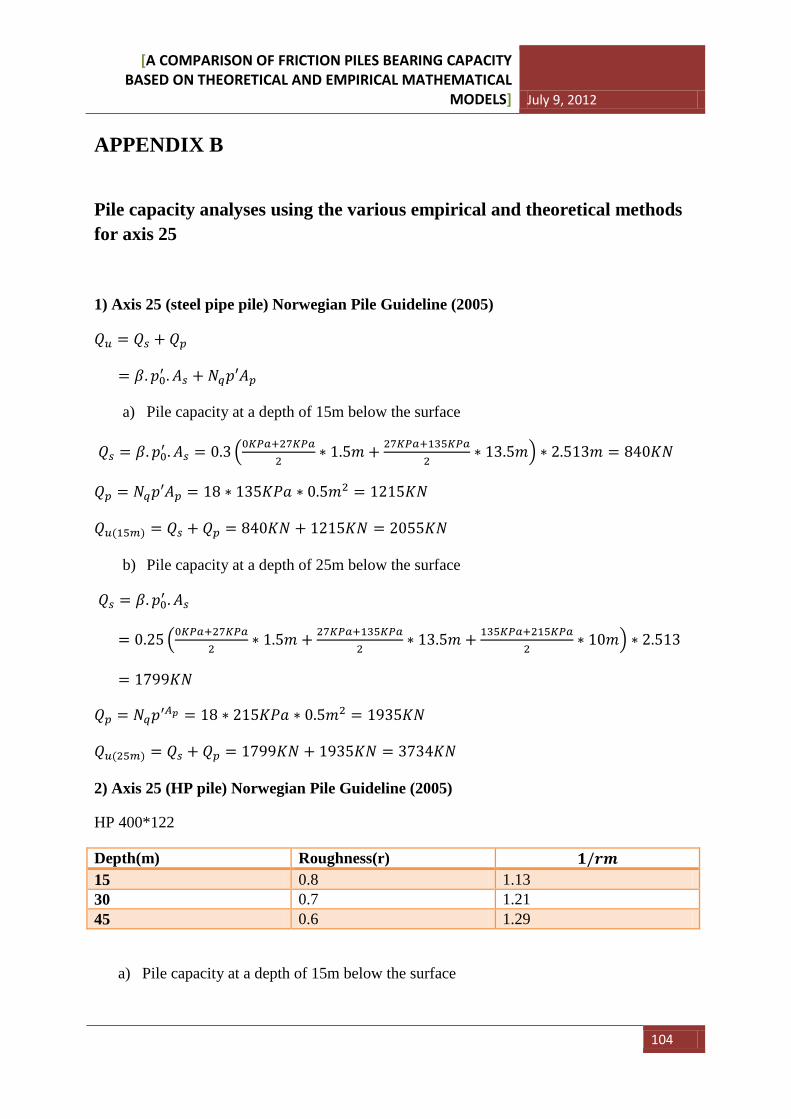
[A COMPARISON OF FRICTION PILES BEARING CAPACITY BASED ON THEORETICAL AND EMPIRICAL MATHEMATICAL
MODELS] July 9, 2012
104
APPENDIX B
Pile capacity analyses using the various empirical and theoretical methods for axis 25
1) Axis 25 (steel pipe pile) Norwegian Pile Guideline (2005)
𝑄𝑢 = 𝑄𝑠 + 𝑄𝑝
= 𝛽.𝑝0′ .𝐴𝑠 + 𝑁𝑞𝑝′𝐴𝑝
a) Pile capacity at a depth of 15m below the surface
𝑄𝑠 = 𝛽.𝑝0′ .𝐴𝑠 = 0.3 �0𝐾𝑃𝑎+27𝐾𝑃𝑎2
∗ 1.5𝑚 + 27𝐾𝑃𝑎+135𝐾𝑃𝑎2
∗ 13.5𝑚� ∗ 2.513𝑚 = 840𝐾𝑁
𝑄𝑝 = 𝑁𝑞𝑝′𝐴𝑝 = 18 ∗ 135𝐾𝑃𝑎 ∗ 0.5𝑚2 = 1215𝐾𝑁
𝑄𝑢(15𝑚) = 𝑄𝑠 + 𝑄𝑝 = 840𝐾𝑁 + 1215𝐾𝑁 = 2055𝐾𝑁
b) Pile capacity at a depth of 25m below the surface
𝑄𝑠 = 𝛽.𝑝0′ .𝐴𝑠
= 0.25 �0𝐾𝑃𝑎+27𝐾𝑃𝑎2
∗ 1.5𝑚 + 27𝐾𝑃𝑎+135𝐾𝑃𝑎2
∗ 13.5𝑚 + 135𝐾𝑃𝑎+215𝐾𝑃𝑎2
∗ 10𝑚� ∗ 2.513
= 1799𝐾𝑁
𝑄𝑝 = 𝑁𝑞𝑝′𝐴𝑝 = 18 ∗ 215𝐾𝑃𝑎 ∗ 0.5𝑚2 = 1935𝐾𝑁
𝑄𝑢(25𝑚) = 𝑄𝑠 + 𝑄𝑝 = 1799𝐾𝑁 + 1935𝐾𝑁 = 3734𝐾𝑁
2) Axis 25 (HP pile) Norwegian Pile Guideline (2005)
HP 400*122
Depth(m) Roughness(r) 𝟏/𝒓𝒎 15 0.8 1.13 30 0.7 1.21 45 0.6 1.29
a) Pile capacity at a depth of 15m below the surface
[A COMPARISON OF FRICTION PILES BEARING CAPACITY BASED ON THEORETICAL AND EMPIRICAL MATHEMATICAL
MODELS] July 9, 2012
105
𝑄𝑠 = 840𝐾𝑁 ∗ 1.476𝑚2.513𝑚
∗ 1.1 = 543𝐾𝑁
𝑄𝑝 = 𝑁𝑞𝑝′𝐴𝑝 = 18 ∗ 135𝐾𝑃𝑎 ∗ 0.136𝑚2 = 330𝐾𝑁
𝑄𝑢(15𝑚) = 𝑄𝑠 + 𝑄𝑝 = 543𝐾𝑁 + 330𝐾𝑁 = 873𝐾𝑁
b) Pile capacity at a depth of 25m below the surface
𝑄𝑠 = 1799𝐾𝑁 ∗ 1.476𝑚2.513𝑚
∗ 1.12 = 1183𝐾𝑁
𝑄𝑝 = 𝑁𝑞𝑝′𝐴𝑝 = 18 ∗ 215𝐾𝑃𝑎 ∗ 0.136𝑚2 = 526𝐾𝑁
𝑄𝑢(25𝑚) = 𝑄𝑠 + 𝑄𝑝 = 1183𝐾𝑁 + 526𝐾𝑁 = 1709𝐾𝑁
3) Axis 25 (steel pipe pile) API RP 2A (2007)
a) Pile capacity at a depth of 15m below the surface
𝑄𝑠 = 𝐾𝑝′𝑡𝑎𝑛𝛿𝐴𝑠
= 1 ∗ �0𝐾𝑃𝑎+27𝐾𝑃𝑎2
∗ 1.5𝑚 + 27𝐾𝑃𝑎+135𝐾𝑃𝑎2
∗ 13.5𝑚� ∗ 2.513𝑚 ∗ 𝑡𝑎𝑛300
= 1616𝐾𝑁
𝑄𝑝 = 𝑁𝑞𝑝′𝐴𝑝 = 40 ∗ 135𝐾𝑃𝑎 ∗ 0.5𝑚2 = 2700𝐾𝑁
𝑄𝑢(15𝑚) = 𝑄𝑠 + 𝑄𝑝 = 1616𝐾𝑁 + 2700𝐾𝑁 = 4316𝐾𝑁
b) Pile capacity at a depth of 25m below the surface
𝑄𝑠 = 𝐾𝑝′𝑡𝑎𝑛𝛿𝐴𝑠
= 1 ∗ �0𝐾𝑃𝑎+27𝐾𝑃𝑎2
∗ 1.5𝑚 + 27𝐾𝑃𝑎+135𝐾𝑃𝑎2
∗ 13.5𝑚 + 135𝐾𝑃𝑎+215𝐾𝑃𝑎2
∗ 10𝑚� ∗ 2.513𝑚 ∗
𝑡𝑎𝑛300
= 4155𝐾𝑁
𝑄𝑝 = 𝑁𝑞𝑝′𝐴𝑝 = 40 ∗ 215𝐾𝑃𝑎 ∗ 0.5𝑚2 = 4300𝐾𝑁
𝑄𝑢(25𝑚) = 𝑄𝑠 + 𝑄𝑝 = 4155𝐾𝑁 + 4300𝐾𝑁 = 8455𝐾𝑁
4) Axis 25 (HP pile) API RP 2A (2007)
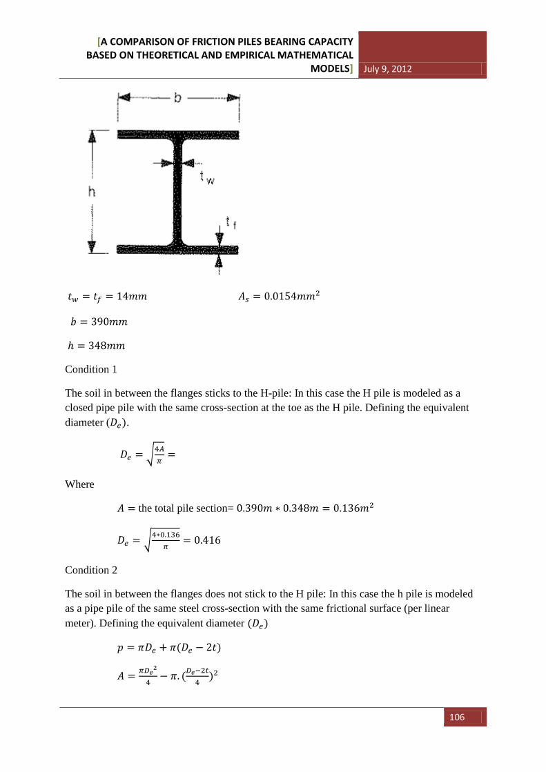
[A COMPARISON OF FRICTION PILES BEARING CAPACITY BASED ON THEORETICAL AND EMPIRICAL MATHEMATICAL
MODELS] July 9, 2012
106
𝑡𝑤 = 𝑡𝑓 = 14𝑚𝑚 𝐴𝑠 = 0.0154𝑚𝑚2
𝑏 = 390𝑚𝑚
ℎ = 348𝑚𝑚
Condition 1
The soil in between the flanges sticks to the H-pile: In this case the H pile is modeled as a closed pipe pile with the same cross-section at the toe as the H pile. Defining the equivalent diameter (𝐷𝑒).
𝐷𝑒 = �4𝐴𝜋
=
Where
𝐴 = the total pile section= 0.390𝑚 ∗ 0.348𝑚 = 0.136𝑚2
𝐷𝑒 = �4∗0.136𝜋
= 0.416
Condition 2
The soil in between the flanges does not stick to the H pile: In this case the h pile is modeled as a pipe pile of the same steel cross-section with the same frictional surface (per linear meter). Defining the equivalent diameter (𝐷𝑒)
𝑝 = 𝜋𝐷𝑒 + 𝜋(𝐷𝑒 − 2𝑡)
𝐴 = 𝜋𝐷𝑒2
4− 𝜋. (𝐷𝑒−2𝑡
4)2
[A COMPARISON OF FRICTION PILES BEARING CAPACITY BASED ON THEORETICAL AND EMPIRICAL MATHEMATICAL
MODELS] July 9, 2012
107
Where
𝑡 = wall thickness
𝑝 = ��390 − (2 ∗ 14)� ∗ 2� + (2 ∗ 390) + (2 ∗ 348) = 2200𝑚𝑚 = 2.2𝑚
𝐴𝑠 = �14 ∗ �348 − (2 ∗ 14)�� + (2 ∗ 390 ∗ 14) = 15400𝑚𝑚2 = 0.0154𝑚2
2.2 = 𝜋𝐷𝑒 + 𝜋(𝐷𝑒 − 2𝑡)……………………... (1)
0.0154 = 𝜋𝐷𝑒2
4− 𝜋. (𝐷𝑒−2𝑡
4)2………………….. (2)
Solving equation 1) and 2) simultaneously we obtain
𝐷𝑒 = 0.3654𝑚
𝑡 = 0.0153𝑚
a) Pile capacity at a depth of 15m below the surface
Condition 1)
𝑄𝑠 = 𝐾𝑝′𝑡𝑎𝑛𝛿𝐴𝑠
= 1 ∗ �0𝐾𝑃𝑎+27𝐾𝑃𝑎2
∗ 1.5𝑚 + 27𝐾𝑃𝑎+135𝐾𝑃𝑎2
∗ 13.5𝑚� ∗ 1.307𝑚 ∗ 𝑡𝑎𝑛300
= 840𝐾𝑁
𝑄𝑝 = 𝑁𝑞𝑝′𝐴𝑝 = 40 ∗ 135𝐾𝑃𝑎 ∗ 0.136𝑚2 = 734𝐾𝑁
𝑄𝑢(15𝑚) = 𝑄𝑠 + 𝑄𝑝 = 840𝐾𝑁 + 734𝐾𝑁 = 1574𝐾𝑁
Condition 2)
𝑄𝑠 = 𝐾𝑝′𝑡𝑎𝑛𝛿𝐴𝑠
= 0.8 ∗ �0𝐾𝑃𝑎+27𝐾𝑃𝑎2
∗ 1.5𝑚 + 27𝐾𝑃𝑎+135𝐾𝑃𝑎2
∗ 13.5𝑚� ∗ 2.2𝑚 ∗ 𝑡𝑎𝑛300
= 1132𝐾𝑁
𝑄𝑝 = 𝑁𝑞𝑝′𝐴𝑝 = 40 ∗ 135𝐾𝑃𝑎 ∗ 0.0154𝑚2 = 83𝐾𝑁
𝑄𝑢(15𝑚) = 𝑄𝑠 + 𝑄𝑝 = 1132𝐾𝑁 + 83𝐾𝑁 = 1215𝐾𝑁
Therefore, Condition to 2 is the governing pile capacity
b) Pile capacity at a depth of 25m below the surface
[A COMPARISON OF FRICTION PILES BEARING CAPACITY BASED ON THEORETICAL AND EMPIRICAL MATHEMATICAL
MODELS] July 9, 2012
108
Condition 1)
𝑄𝑠 = 𝐾𝑝′𝑡𝑎𝑛𝛿𝐴𝑠
= 1 ∗ �0𝐾𝑃𝑎+27𝐾𝑃𝑎2
∗ 1.5𝑚 + 27𝐾𝑃𝑎+135𝐾𝑃𝑎2
∗ 13.5𝑚 + 135𝐾𝑃𝑎+215𝐾𝑃𝑎2
∗ 10𝑚� ∗ 1.307𝑚 ∗
𝑡𝑎𝑛300
= 2161𝐾𝑁
𝑄𝑝 = 𝑁𝑞𝑝′𝐴𝑝 = 40 ∗ 215𝐾𝑃𝑎 ∗ 0.136𝑚2 = 1170𝐾𝑁
𝑄𝑢(25𝑚) = 𝑄𝑠 + 𝑄𝑝 = 2161𝐾𝑁 + 1170𝐾𝑁 = 3331𝐾𝑁
Condition 2)
𝑄𝑠 = 𝐾𝑝′𝑡𝑎𝑛𝛿𝐴𝑠
= 0.8 ∗ �0𝐾𝑃𝑎+27𝐾𝑃𝑎2
∗ 1.5𝑚 + 27𝐾𝑃𝑎+135𝐾𝑃𝑎2
∗ 13.5𝑚 + 135𝐾𝑃𝑎+215𝐾𝑃𝑎2
∗ 10𝑚� ∗ 2.2𝑚 ∗
𝑡𝑎𝑛300
= 2910𝐾𝑁
𝑄𝑝 = 𝑁𝑞𝑝′𝐴𝑝 = 40 ∗ 215𝐾𝑃𝑎 ∗ 0.0154𝑚2 = 132𝐾𝑁
𝑄𝑢(25𝑚) = 𝑄𝑠 + 𝑄𝑝 = 2910𝐾𝑁 + 132𝐾𝑁 = 3042𝐾𝑁
Therefore, Condition to 2 is the governing capacity
5) Axis 25 (steel pipe) Janbu Theoretical
a) Pile capacity at a depth of 15m below the surface
From chart;
𝑡𝑎𝑛𝜑 = 0.7, 𝑟 = 0.8 → 𝑆𝑣 = 0.24
𝑡𝑎𝑛𝜑 = 0.7, 𝛽 = 0 → 𝑁𝑞 = 30
𝑄𝑠 = 𝑆𝑣(𝑝′ + 𝑎)𝐴𝑠
= 0.24 �0𝐾𝑃𝑎+27𝐾𝑃𝑎2
∗ 1.5𝑚 + 27𝐾𝑃𝑎+135𝐾𝑃𝑎2
∗ 13.5𝑚� ∗ 2.513𝑚 = 672𝐾𝑁
𝑄𝑝 = �𝑁𝑞 − 1�(𝑝′ + 𝑎)𝐴𝑝 = (30 − 1) ∗ 135𝐾𝑃𝑎 ∗ 0.5𝑚2 = 1958𝐾𝑁
𝑄𝑢(15𝑚) = 𝑄𝑠 + 𝑄𝑝 = 672𝐾𝑁 + 1958𝐾𝑁 = 2630𝐾𝑁
b) Pile capacity at a depth of 25m below the surface
[A COMPARISON OF FRICTION PILES BEARING CAPACITY BASED ON THEORETICAL AND EMPIRICAL MATHEMATICAL
MODELS] July 9, 2012
109
𝑡𝑎𝑛𝜑 = 0.7, 𝑟 = 0.7 → 𝑆𝑣 = 0.18
𝑡𝑎𝑛𝜑 = 0.7, 𝛽 = 0 → 𝑁𝑞 = 30
𝑄𝑠 = 𝑆𝑣(𝑝′ + 𝑎)𝐴𝑠
= 0.24 �0𝐾𝑃𝑎+27𝐾𝑃𝑎2
∗ 1.5𝑚 + 27𝐾𝑃𝑎+135𝐾𝑃𝑎2
∗ 13.5𝑚 + 135𝐾𝑃𝑎+215𝐾𝑃𝑎2
∗ 10𝑚� ∗ 2.513𝑚
= 1295𝐾𝑁
𝑄𝑝 = �𝑁𝑞 − 1�(𝑝′ + 𝑎)𝐴𝑝 = (30 − 1) ∗ 215𝐾𝑃𝑎 ∗ 0.5𝑚2 = 3118𝐾𝑁
𝑄𝑢(25𝑚) = 𝑄𝑠 + 𝑄𝑝 = 1295𝐾𝑁 + 3118𝐾𝑁 = 4412𝐾𝑁
6) Axis 25 (HP pile) Janbu theoretical
a) Pile capacity at a depth of 15m below the surface
𝑄𝑠 = 672𝐾𝑁 ∗ 1.476𝑚2.513𝑚
∗ 1.1 = 434𝐾𝑁
𝑄𝑝 = (30 − 1) ∗ 135𝐾𝑃𝑎 ∗ 0.136𝑚2 = 532𝐾𝑁
𝑄𝑢(15𝑚) = 𝑄𝑠 + 𝑄𝑝 = 434𝐾𝑁 + 532𝐾𝑁 = 966𝐾𝑁
b) Pile capacity at a depth of 25m below the surface
𝑄𝑠 = 1295𝐾𝑁 ∗ 1.476𝑚2.513𝑚
∗ 1.12 = 852𝐾𝑁
𝑄𝑝 = (30 − 1) ∗ 215𝐾𝑃𝑎 ∗ 0.136𝑚2 = 848𝐾𝑁
𝑄𝑢(25𝑚) = 𝑄𝑠 + 𝑄𝑝 = 852𝐾𝑁 + 848𝐾𝑁 = 1700𝐾𝑁
7) Axis 25 (steel pipe) NGI-99
a) Pile capacity at a depth of 15m below the surface
𝐷𝑟 = 0.4. 𝑙𝑛 �𝑞𝑐 [22. (𝜎′𝑣0.𝜎𝑎𝑡𝑚)0.5]� � = 0.4. 𝑙𝑛 �7100𝐾𝑃𝑎[22. (100𝐾𝑃𝑎. 75𝐾𝑃𝑎)0.5]� �
𝐷𝑟 = 0.52
𝐹𝐷𝑟 = 2.1. (𝐷𝑟 − 0.1)1.7 = 2.1. (0.52 − 0.1)1.7 = 0.48
𝐹𝑠𝑖𝑔 = (𝜎′𝑣0
𝜎𝑎𝑡𝑚)0.25 = � 75𝐾𝑃𝑎
100𝐾𝑃𝑎�0.25
= 0.93
𝐹𝑡𝑖𝑝 = 1.6 = (closed ended)
[A COMPARISON OF FRICTION PILES BEARING CAPACITY BASED ON THEORETICAL AND EMPIRICAL MATHEMATICAL
MODELS] July 9, 2012
110
𝐹𝑙𝑜𝑎𝑑 = 1.3= (compression load)
𝐹𝑚𝑎𝑡 = 1.0 = (steel)
𝑄𝑠 = 𝑧𝑧𝑡𝑖𝑝
∗ 𝜎𝑎𝑡𝑚 ∗ 𝐹𝐷𝑟 ∗ 𝐹𝑠𝑖𝑔 ∗ 𝐹𝑡𝑖𝑝 ∗ 𝐹𝑙𝑜𝑎𝑑 ∗ 𝐹𝑚𝑎𝑡 ∗ 𝐴𝑠
=7.5𝑚15𝑚
∗ 100𝐾𝑝𝑎 ∗ 0.48 ∗ 0.93 ∗ 1.6 ∗ 1.3 ∗ 1.0 ∗ 2.513𝑚 ∗ 15𝑚 = 1750𝐾𝑁
𝑄𝑝 = 0.8 𝑞𝑐(1+𝐷𝑟2)
𝐴𝑝
= 0.8 ∗ 7100𝐾𝑃𝑎(1+0.522)
∗ 0.5𝑚2 = 2204𝐾𝑁
𝑄𝑢(15𝑚) = 𝑄𝑠 + 𝑄𝑝 = 1750𝐾𝑁 + 2204𝐾𝑁 = 3954𝐾𝑁
b) Pile capacity at a depth of 25m below the surface
𝐷𝑟 = 0.4. 𝑙𝑛 �7100𝐾𝑃𝑎[22. (100𝐾𝑃𝑎. 115𝐾𝑃𝑎)0.5]� � = 0.44
𝐹𝐷𝑟 = 2.1. (𝐷𝑟 − 0.1)1.7 = 2.1. (0.44 − 0.1)1.7 = 0.33
𝐹𝑠𝑖𝑔 = (𝜎′𝑣0
𝜎𝑎𝑡𝑚)0.25 = �115𝐾𝑃𝑎
100𝐾𝑃𝑎�0.25
= 1.035
𝑄𝑠 = 12.5𝑚25𝑚
∗ 100𝐾𝑝𝑎 ∗ 0.33 ∗ 1.035 ∗ 1.6 ∗ 1.3 ∗ 1.0 ∗ 2.513𝑚 ∗ 25𝑚 = 2232𝐾𝑁
𝑄𝑝 = 0.8 ∗ 7100𝐾𝑃𝑎(1+0.442)
∗ 0.5𝑚2 = 2346𝐾𝑁
𝑄𝑢(25𝑚) = 𝑄𝑠 + 𝑄𝑝 = 2232𝐾𝑁 + 2346𝐾𝑁 = 4578𝐾𝑁
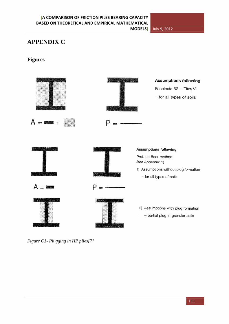
[A COMPARISON OF FRICTION PILES BEARING CAPACITY BASED ON THEORETICAL AND EMPIRICAL MATHEMATICAL
MODELS] July 9, 2012
111
APPENDIX C
Figures
Figure C1- Plugging in HP piles[7]
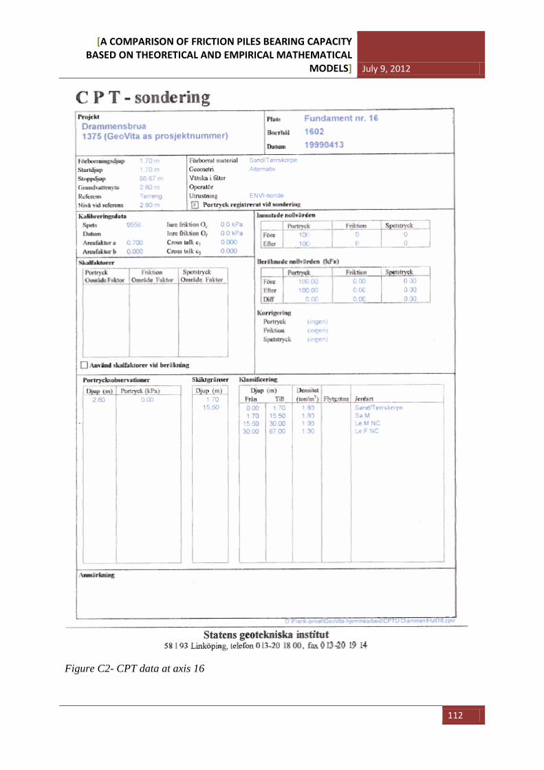
[A COMPARISON OF FRICTION PILES BEARING CAPACITY BASED ON THEORETICAL AND EMPIRICAL MATHEMATICAL
MODELS] July 9, 2012
112
Figure C2- CPT data at axis 16
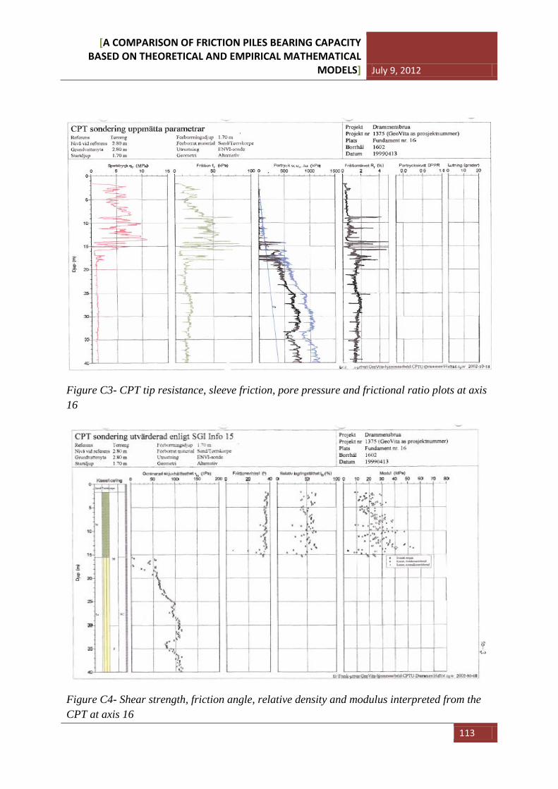
[A COMPARISON OF FRICTION PILES BEARING CAPACITY BASED ON THEORETICAL AND EMPIRICAL MATHEMATICAL
MODELS] July 9, 2012
113
Figure C3- CPT tip resistance, sleeve friction, pore pressure and frictional ratio plots at axis 16
Figure C4- Shear strength, friction angle, relative density and modulus interpreted from the CPT at axis 16
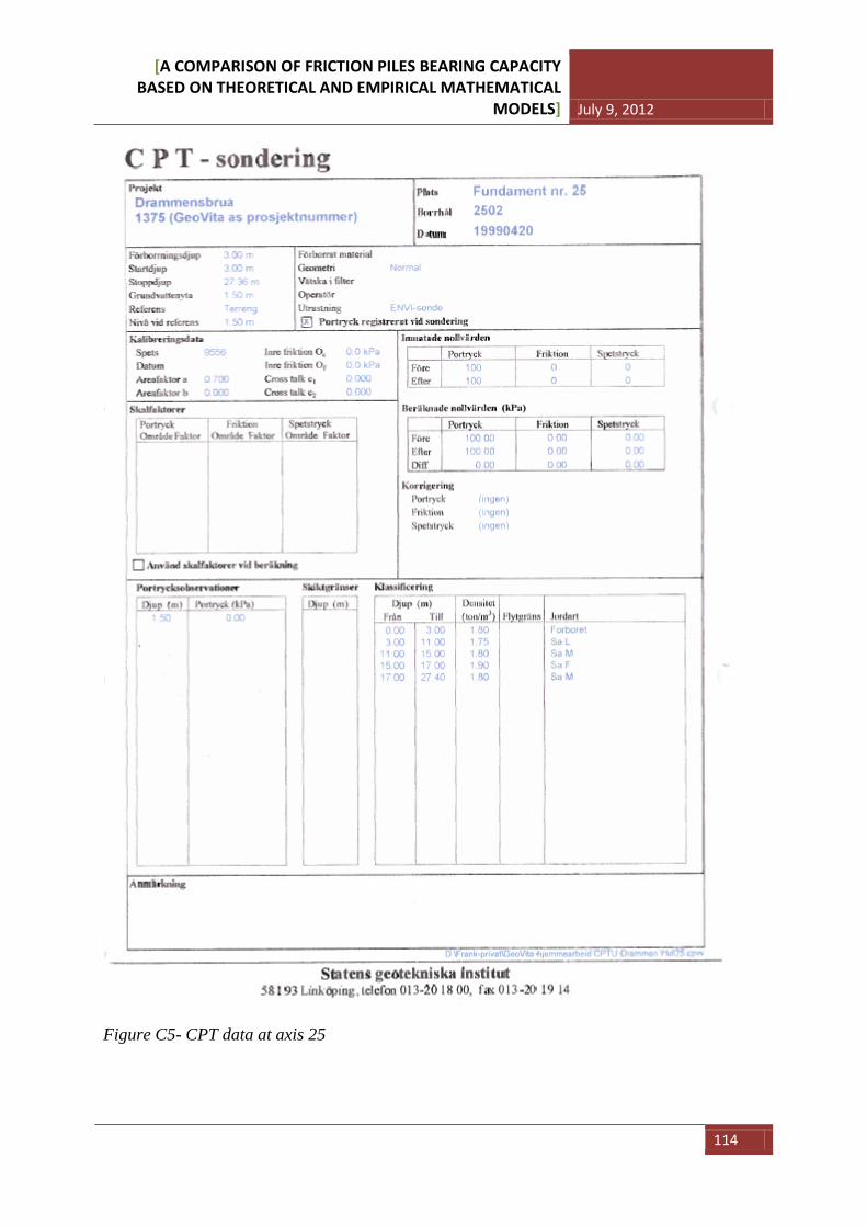
[A COMPARISON OF FRICTION PILES BEARING CAPACITY BASED ON THEORETICAL AND EMPIRICAL MATHEMATICAL
MODELS] July 9, 2012
114
Figure C5- CPT data at axis 25
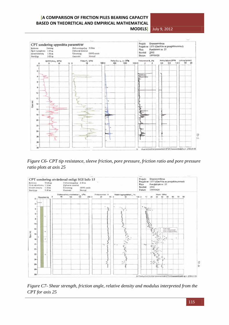
[A COMPARISON OF FRICTION PILES BEARING CAPACITY BASED ON THEORETICAL AND EMPIRICAL MATHEMATICAL
MODELS] July 9, 2012
115
Figure C6- CPT tip resistance, sleeve friction, pore pressure, friction ratio and pore pressure ratio plots at axis 25
Figure C7- Shear strength, friction angle, relative density and modulus interpreted from the CPT for axis 25
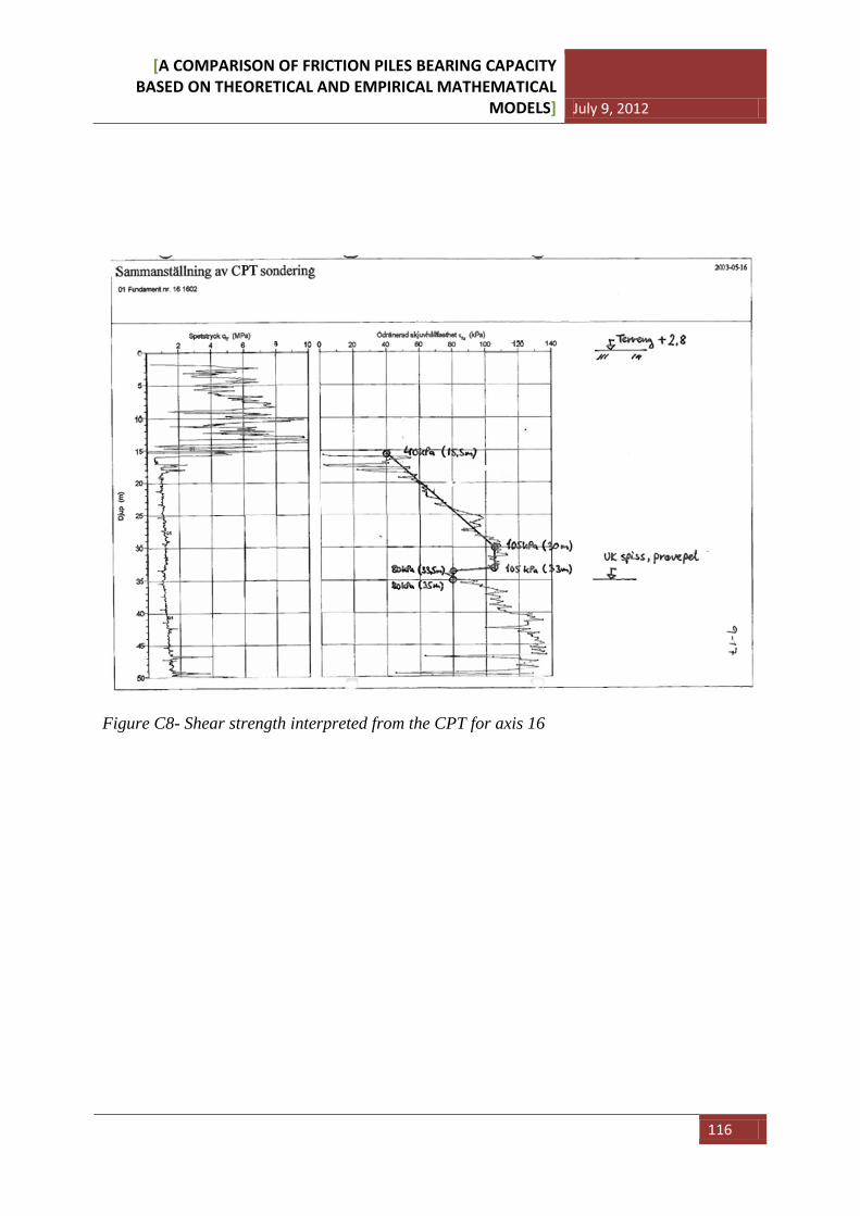
[A COMPARISON OF FRICTION PILES BEARING CAPACITY BASED ON THEORETICAL AND EMPIRICAL MATHEMATICAL
MODELS] July 9, 2012
116
Figure C8- Shear strength interpreted from the CPT for axis 16