1. I ntroduction

A Comparison of Complementaryand Kalman Filtering

WALTER T. HIGGINS, JR.Member, IEEEArizona State UniversityTempe, Ariz. 85281

Abstract

A technique used in the flight control industry for estimation when

combining measurements is the complementary filter. This filter isusually designed without any reference to Wiener or Kalman filters,

although it is related to them. This paper, which is mainly tutorial,reviews complementary filtering and shows its relationship to Kal-

man and Wiener filtering.

A simple estimation technique that is often used in theflight control industry to combine measurements is thecomplementary filter [1]. This filter is actually a steady-state Kalman filter (i.e., a Wiener filter) for a certain classof filtering problems. This relationship does not appear tobe well known by many practitioners of either comple-mentary or Kalman filtering. One exception is the tutorialpaper by Brown [2] which discusses this relationshipwithout going into the mathematical details.

The complementary filter users do not consider anystatistical description for the noise corrupting the signals,and their filter is obtained by a simple analysis in the fre-quency domain. The proponents of the Kalman filteringapproach work in the time domain and do not pay muchattention to the transfer function or frequency domain(Wiener filter) approach to the filtering problem, since it isa less general approach to the filtering problem. TheWiener filter solution to this class of multiple-input estima-tion problems appeared in the literature [3], [4] well be-fore Kalman published his classic paper [5].

This paper reviews complementary filtering and showshow this technique is related to Kalman and Wiener filter-ing. Since both Kalman and complementary filtering areunder consideration for use in the Space Shuttle Reentryand Landing Navigation System, the relationship betweenthem should be well understood.

11. Complementary Filtering

Manuscript received August 6, 1974; revised December 27, 1974.Copyright 1975 by IEEE Thans. Aerospace and Electronic Systems,Vol. AES-li, no. 3, May 1975.

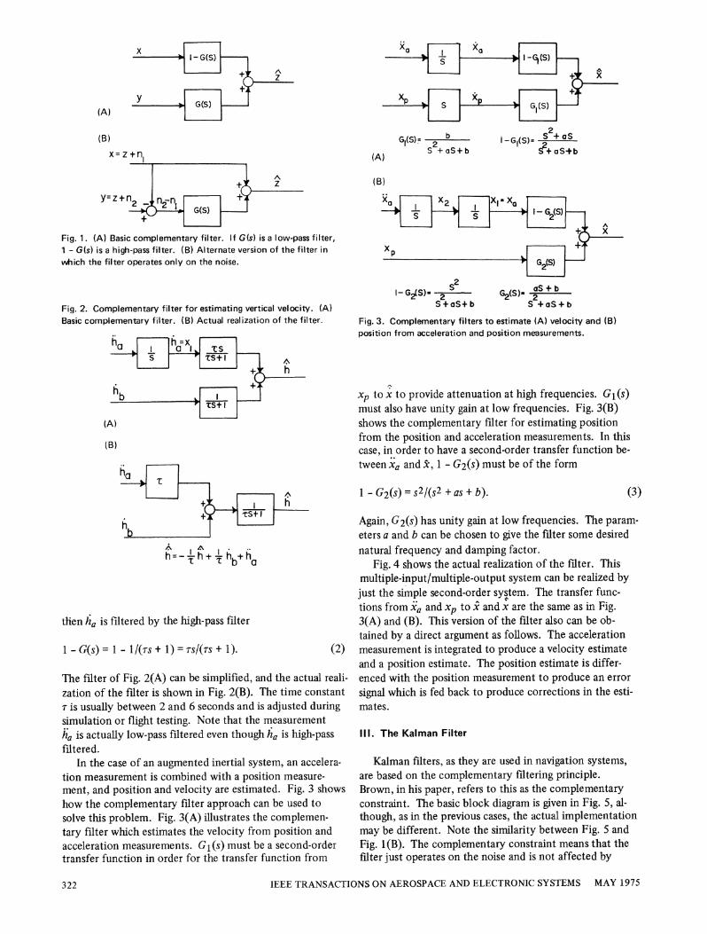
The basic complementary filter is shown in Fig. 1(A)where x and y are noisy measurements of some signal z andz is the estimate of z produced by the filter. Assume thatthe noise in y is mostly high frequency, and the noise in xis mostly low frequency. Then G(s) can be made a low-pass filter to filter out the high-frequency noise in y. IfG(s) is low-pass, [1 - G(s)] is the complement, i.e., a high-pass filter which filters out the low-frequency noise in x.No detailed description of the noise processes are consid-ered in complementary filtering.

The complementary filter can be reconfigured as inFig. 1(B). In this case the input to G(s) is y - x = n2 - n I,so that the filter G(s) just operates on the noise or error inthe measurements x and y. Note that, in the case of noise-less or error-free measurements, z = z [1 - G(s)] + zG(s) =z; i.e., the signal is estimated perfectly.A typical application of the complementary filter is to

combine measurements of vertical acceleration and baro-metric vertical velocity to obtain an estimate of verticalvelocity. To fit the previous discussion, assume that theacceleration measurement is integrated to produce a veloc-ity signal ha, as shown in Fig. 2. The integration attenu-ates the high-frequency noise in the acceleration measure-ment, whereas the noise in hb is not changed. Therefore, ifhb is filtered by the low-pass filter

G(s) = 1/(rs + 1), (1)

IEEE TRANACTIONS ON AEROSPACE AND ELECTRONIC SYSTEMS VOL. AES-1 1, NO. 3 MAY 1975 321

(A)

(B)

Az

+I- IFig. 1. (A) Basic complementary filter. If G(s) is a low-pass filter,1 - G(s) is a high-pass filter. (B) Alternate version of the filter inwhich the filter operates only on the noise.

Fig. 2. Complementary filter for estimating vertical velocity. (A)Basic complementary filter. (B) Actual realization of the filter.

(A)

(B)

^ A .h= y h + y hbiha

thten ha is filtered by the high-pass filter

1 - G(s) = 1 - l/(Ts + 1) = TS/(TS + 1). (2)

The filter of Fig. 2(A) can be simplified, and the actual reali-zation of the filter is shown in Fig. 2(B). The time constantT is usually between 2 and 6 seconds and is adjusted duringsimulation or flight testing. Note that the measurementha is actually low-pass filtered even though ha is high-passfiltered.

In the case of an augmented inertial system, an accelera-tion measurement is combined with a position measure-ment, and position and velocity are estimated. Fig. 3 showshow the complementary filter approach can be used tosolve this problem. Fig. 3(A) illustrates the complemen-tary filter which estimates the velocity from position andacceleration measurements. Gl(s) must be a second-ordertransfer function in order for the transfer function from

(A)

(B)

b KG(S)- S +aS=2 S -I(SS +aS+b S2+ S+b

2 G252(S) aS2S+aS+b S +aS+b

Fig. 3. Complementary filters to estimate (A) velocity and (B)position from acceleration and position measurements.

xp to x to provide attenuation at high frequencies. G1(s)must also have unity gain at low frequencies. Fig. 3(B)shows the complementary filter for estimating positionfrom the position and acceleration measurements. In thiscase, in order to have a second-order transfer function be-tween xa and x, 1 - G2(s) must be of the form

1 - G2(s) = s2/(s2 + as + b). (3)

Again, G2(s) has unity gain at low frequencies. The param-eters a and b can be chosen to give the filter some desirednatural frequency and damping factor.

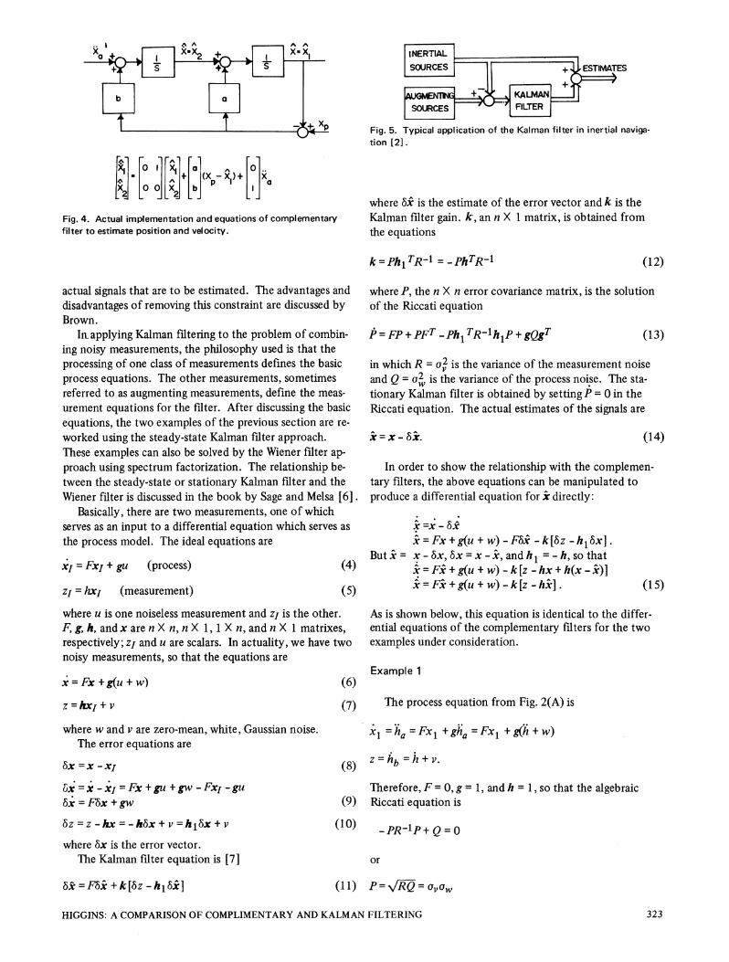
Fig. 4 shows the actual realization of the filter. Thismultiple-input/multiple-output system can be realized byjust the simple second-order system. The transfer func-tions from xa and xp to x and x are the same as in Fig.3(A) and (B). This version of the filter also can be ob-tained by a direct argument as follows. The accelerationmeasurement is integrated to produce a velocity estimateand a position estimate. The position estimate is differ-enced with the position measurement to produce an errorsignal which is fed back to produce corrections in the esti-mates.

Ill. The Kalman Filter

Kalman filters, as they are used in navigation systems,are based on the complementary filtering principle.Brown, in his paper, refers to this as the complementaryconstraint. The basic block diagram is given in Fig. 5, al-though, as in the previous cases, the actual implementationmay be different. Note the similarity between Fig. 5 andFig. 1(B). The complementary constraint means that thefilter just operates on the noise and is not affected by

IEEE TRANSACTIONS ON AEROSPACE AND ELECTRONIC SYSTEMS MAY 1975322

|SOURCES ESTIMATES

:~~~~~~~~~~~~~~~~~~~|SOURCES FITE

Fig. 5. Typical application of the Kalman filter in inertial naviga-tion [2].

RI X1[ ] [a1 A °1

Fig. 4. Actual implementation and equations of complementaryfilter to estimate position and velocity.

where 6k is the estimate of the error vector and k is theKalman filter gain. k, an n X 1 matrix, is obtained fromthe equations

k =Ph1 TR-1 = - PhTR-l (12)

actual signals that are to be estimated. The advantages anddisadvantages of removing this constraint are discussed byBrown.

hInapplying Kalman filtering to the problem of combin-ing noisy measurements, the philosophy used is that theprocessing of one class of measurements defines the basicprocess equations. The other measurements, sometimesreferred to as augmenting measurements, define the meas-urement equations for the filter. After discussing the basicequations, the two examples of the previous section are re-worked using the steady-state Kalman filter approach.These examples can also be solved by the Wiener filter ap-proach using spectrum factorization. The relationship be-tween the steady-state or stationary Kalman filter and theWiener filter is discussed in the book by Sage and Melsa [6].

Basically, there are two measurements, one of whichserves as an input to a differential equation which serves asthe process model. The ideal equations are

XI = Fxj + gu (process)

zj = hxj (measurement)

(4)

(5)

where P, the n X n error covariance matrix, is the solutionof the Riccati equation

P = FP +PFT - Ph TR-h1p+gQgT (13)

in which R = u2 is the variance of the measurement noiseand Q = u2 is the variance of the process noise. The sta-tionary Kalman filter is obtained by setting P = 0 in theRiccati equation. The actual estimates of the signals are

x=x- x. (14)

In order to show the relationship with the complemen-tary filters, the above equations can be manipulated toproduce a differential equation for x directly:

x =x -6*xx=Fx+g(u + w) -FA -k[6z -h,6x].

Butk= x - Ax,6x = x -i, andhi = -h, so thatx = Fk + g(u + w) - k [z - hx + h(x - x)]x = Fk + g(u + w) - k[z - hx].

where u is one noiseless measurement and zj is the other.F, g, h, andx are n X n, n X 1, 1 X n, and n X I matrixes,respectively; zj and u are scalars. In actuality, we have twonoisy measurements, so that the equations are

x = Fx + g(u + w)

z =hxj + v

where w and v are zero-mean, white, Gaussian noise.The error equations are

Ax =x -XI

X= X -X= Fx +gu +gw - Fx1 -gu6x = F8x + gw

6z = z -hx = -hbx +1v =hlx + v

where 6x is the error vector.The Kalman filter equation is [7]

x6 =F~x +k[6z -hl x6]

(6)

(7)

(8)

As is shown below, this equation is identical to the differ-ential equations of the complementary filters for the twoexamples under consideration.

Example 1

The process equation from Fig. 2(A) is

xi =k =Fxl +gh, =Fxj +g(h+w)

Z=hb =h + v.

Therefore, F = 0, g = 1, and h = 1, so that the algebraic(9) Riccati equation is

(10) -PR-lP+ Q = 0

or

(11) P=V-=aa,

HIGGINS: A COMPARISON OF COMPLIMENTARY AND KALMAN FILTERING

(15)

323

assumption that the measurements are corrupted by sta-tionary white noise produces a stationary Kalman filterthat is identical in form to the complementary filter.

The filter equation is obtained by substituting into (15):

x ha + (wlav) [hb-X]

x=(-ow lav)xi + (awulav)hb +ha (16

This equation is identical to the equation of the comple-mentary filter in Fig. 2(B), where the time constant of thefilter is now r = a,/ow Note that a time constant of four,as in the complementary filter, means that the barometricsignal is assumed to be much noisier than the accelerome-ter signal. In the complementary filter, the time constantis chosen to get most of the information from the accelero-meter signal and use the barometric information only as along-term reference.

Example 2

The process equation from Fig. 3(B) is

KlX ] FF[olX[!]L=X$LX1i=Li[i]+[jY.w

IV. Digital Implementation

Since modern inertial navigation systems use digital com-puters, the continuous filters can be replaced by discrete

) approximations, or the problem can be formulated as asampled measurement problem from the start. The com-plementary or stationary Kalman filter has a considerableadvantage over the normal Kalman filter because the Ric-cati equation and Kalman gains are not computed. There-fore, the update rate of the complementary filter can behigher than the normal Kalman filter. This is an importantconsideration in the applications to automatic landingproblems, especially in an unpowered vehicle, such as thespace shuttle, which has a rapid descent rate before finalflare.

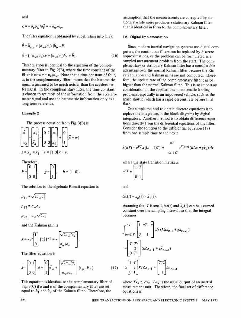
One simple method to obtain discrete equations is toreplace the integrators in the block diagrams by digitalintegrators. Another method is to obtain difference equa-tions directly from the differential equations of the filter.Consider the solution to the differential equation (17)from one sample time to the next:

i(nT) = eFTx[(n - 1)7] +nT

eF(t-) (kAx +gx,) dr(n-l)T

Therefore,

F=[ ] g= h=[l 0].

The solution to the algebraic Riccati equation is

Pi1 = /2u u3

P12 = UcwJv

P22 = gw 2av

and the Kalman gain is

L 2aw/lavk= _ P [av2]-1 = _

The filter equation is

X=; X+ uxa + (x; P -X 1) (IL0 0 1 aw /Or

This equation is identical to the complementary filter ofFig. 3(C) if a and b of the complementary filter are setequal to k, and k2 of the Kalman filter. Therefore, the

where the state transition matrix isI T

eFT =

LO 1

and

Ax(t) =x14t) - x(t).Assuming that T is small, Ax(t) and x, (t) can be assumedconstant over the sampling interval, so that the integralbecomes

nT -r

L ] dr(kAxn-1 +gxan-)(n-1)T 0 1

T T2.L 2 (kAx1n- +gxan-1)0 T

1T ~~T/217) L 2 kTAxn-1 + [T2vxnfl

where Txa - Avx . Avx is the usual output of an inertialmeasurement unit. Therefore, the final set of differenceequations is

IEEE TRANSACTIONS ON AEROSPACE AND ELECTRONIC SYSTEMS MAY 1975

and

k = - a Uv la 2 = - orv v w lav -

324

T T1/T 2

Xn=[l0 1 n-i + 01]kTAxn-1 + [11 Av1n-

V. Conclusions

The relationship between the complementary filter andthe Kalman filter has been shown. The complementaryfilter is simpler because it involves less computation. Thequestion that remains to be answered is how does the ac-

curacy of the two techniques compare? Does the use offixed or preprogrammed gains degrade the filter perform-ance significantly? In idealized cases, as the examples inthis paper, the mean-squared error for given white-noise in-puts can be compared. However, in a specific real-worldproblem, the noise is not really white, the position meas-

urement is a nonlinear function of certain ranges andangles, and the filter equations are higher order, since thereare three positions and velocities to be determined. A truecomparison of the two filters would probably involve an

extensive Monte Carlo simulation.

References

[1] S.S. Osder, W.E. Rouse, and L.S. Young, "Navigation, guid-ance and control systems for V/STOL aircraft," Sperry Tech.vol. 1, no. 3, 1973.

[2] R.G. Brown, "Integrated navigation systems and Kalmanfiltering: a perspective," Navigation, J. Inst. Navigation, vol.19, no. 4, pp. 355-362, Winter 1972-73.

[3] R.M. Stewart and R.J. Parks, "Degenerate solutions andalgebraic approach to the multiple input linear filter designproblems," IRE Trans. Circuit Theory, vol. CT4, pp. 10-14,1957.

[4] J.S. Bendat, "Optimum filters for independent measurementsof two related perturbed messages," IRE Trans. Circuit Theory,vol. CT-4, pp. 14-19, 1957.

[5] R.E. Kalman, "A new approach to linear filtering and predic-tion problems," Trans. ASME, J. Basic Engrg., vol. 82D, pp.3445, March 1960.

[6] A.P. Sage and J.L. Melsa, Estimation Theory with Applicationsto Communications and Control. New York: McGraw-Hill,1971.

[7] J.S. Meditch, Stochastic Optimal Linear Estimation and Con-trol. New York: McGraw-Hill, 1969.

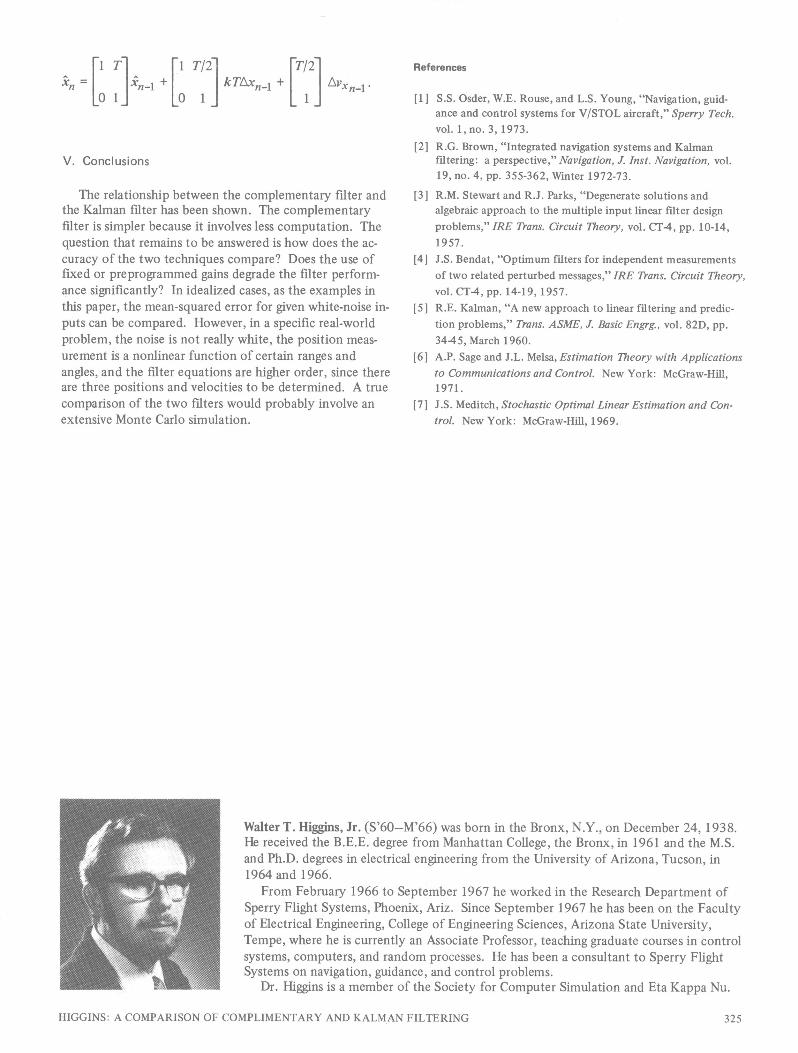
Walter T. Higgins, Jr. (S'60-M'66) was born in the Bronx, N.Y., on December 24, 1938.He received the B.E.E. degree from Manhattan College, the Bronx, in 1961 and the M.S.and Ph.D. degrees in electrical engineering from the University of Arizona, Tucson, in1964 and 1966.

From February 1966 to September 1967 he worked in the Research Department ofSperry Flight Systems, Phoenix, Ariz. Since September 1967 he has been on the Facultyof Electrical Engineering, College of Engineering Sciences, Arizona State University,Tempe, where he is currently an Associate Professor, teaching graduate courses in controlsystems, computers, and random processes. He has been a consultant to Sperry FlightSystems on navigation, guidance, and control problems.

Dr. Higgins is a member of the Society for Computer Simulation and Eta Kappa Nu.

HIGGINS: A COMPARISON OF COMPLIMENTARY AND KALMAN FILTERING 325