POEF-LMUS-87

L O C K H E E D M A R T I N * A Comparison of

Attribute Sampling Plans

J ~ J W 0 4 M97 Brian M. Laming

O S T I

May 1997

MSfRlBUTtdN O f THIS DOCUMENT tS U N t l M ~

NOTICE

This report was prepared as an account of work sponsored by an agency of the United States Government. Neither the United States Government nor any agency thereof, nor any of their employees, makes any warranty, express or implied, or assumes any legd liability or responsibility for the accuracy, completeness, or usefulness of any information, apparatus, product, or process disclosed, or represents that its use would not infringe privately owned rights. Reference herein to any specific commercial pro- duct, process, or service by trade name, trademark, manufacturer, or otherwise, does not necessarily constitute or imply its endorsement, re- commendation, or favoring by the United States Government or any agency thereof. The views and opinions of authors expressed herein do not necessarily state or reflect those of the United States Government or any agency thereof.

This report has been reproduced directly from the best available copy.

Available to Doe and DOE contractors from the Oftice of Scientific and Technical Information, P. 0. Box 62, Oak Ridge, TN 37831; prices available from (423) 576-840 1.

Available to the public from the National Technical Information Service, U. S. Department of Commerce, 5285 Port Royal Rd., Springfield, VA 22161.

Portions of this document may be illegible in electronic image produds Images are produced from the best available original dorlmrent.

BY Brian M. Laming

May 1997

DISCLAIMER

This report was prepared as an account of work sponsored by an agency of the United States Government. Neither the United States Government nor any agency thereof, nor any of their employees, makes any warranty, express or implied, or assumes any legal liability or responsi- bility for the accuracy, completeness, or usefulness of any information, apparatus, product, or process disclosed, or represents that its use would not infringe privately owned rights. Refer- ence herein to any specific commercial product, process, or service by trade name, trademark, manufacturer, or otherwise does not necessarily constitute or imply its endorsement, recom- mendation, or favoring by the United States Government or any agency thereof. The views and opinions of authors expressed herein do not necessarily state or reflect those of the United States Government or any agency thereof.

A Comparison of Attribute Sampling Plans

LOCKHEED MARTIN UTILITY SERVICES, INC. Portsmouth Gaseous Diffusion Plant P.O. Box 628 Piketon, Ohio 45661

POEF-LMUS-87

Under Contract USEC-96-C-000 1 to the

UNITED STATES ENRICHMENT CORPORATION

A COMPARISON OF ATTRIBUTE SAMPLING PLANS

I. ABSTRACT

This report describes, compares, and provides sample size selection criteria for the most common sampling plans for attribute data (i.e., data that is qualitative in nature such as Pass-Fail, Yes- No, Defect-Nondefect data).

This report is being issued as a guide in prudently choosing the correct sampling plan to meet statistical plan objectives.

11. IN!PRODUCTION

In plans based on attributes, consideration is given only to the number of items in the sample conforming or failing to conform to certain quality specifications. This conformance generally relates to a single quality characteristic of the item.

Whenever a decision is based upon a sample size (versus 100% inspection of a population of items) there are risks that the decision will be an incorrect one. So, why not just examine the total population? This will obviously provide risk-free results, however, time and cost usually prevent such an extensive evaluation and thus a sampling plan is utilized.

Sampling plans minimize the amount of inspection required by sampling only a fraction of the population. The information in the sample is then used to make inferences about what's in the total population. A sampling plan shpuld be employed if and only if the auditor and auditee are willing to accept the risks associated with the particular sampling plan. Sampling risks cannot be avoided as long as samples are employed as the basis for decision making.

111. SPECIFYING SAMPLING RISKS

Sampling only a fraction of the population and applying statistical tests to these samples creates two kinds of risks. There is a risk of rejecting a population of acceptable quality. There is also the risk of accepting a population of unacceptable quality. Paramount to employing any sampling plan, then, is awareness of the magnitude of the r i s k s for the given sampling plan. The notation given below is necessary in developing a quality sampling plan and specifying the risks that will be utilized.

Notation

AQL - Acceptable quality level expressed as a percent. a - the chance of rejecting a population of acceptable quality. Commonly

known as the "producers risk". 1-a - the chance of accepting a population of acceptable quality. RQL - Rejectable quality level expressed as a percent. B - the chance of accepting a population of unacceptable quality.

Commonly known as the "consumers" risk. 1-B - the chance of rejecting a population of unacceptable quality. c - acceptance number, the maximum allowable number of defectives in a

sample of size n allowed to accept the population. More than c defectiveswill cause rejection ofthe population. Often c is specified as zero.

n - Sample size. The number of items in the sample. N - Population size. The number of items in the lot, batch, etc.

IV. TYPES OF SAMPLING PLANS AVAILABLE

Sampling plans exist that emphasize only the AQL risk; this means that the main emphasis is placed on minimizing the risk of rejecting items of good quality (AQL or better quality). For example, an auditor might wish to reject a population only a = 5% of the time when the AQL is 1% or better (or equivalently, accept the population 95% of the time when the AQL is 1% o r better). The plan does not control the B risk and thus can result in accepting poor quality populations (i.e., populations with a nonconformance rate worse than the A Q L ) .

Sampling plans also exist that emphasize only the RQL risk; this means that the main emphasis is placed on minimizing the risk of accepting items of poor quality (RQL or worse quality). For example, the auditor might wish to accept a population only B = 5% of the time when the RQL is 1% or worse (or equivalently, reject the population 95% of the time when the RQL is 1% or worse). The plan does not control the a risk and thus can result in rejecting acceptable quality populations (io@., rejecting populations with a nonconformance rate better than the R Q L ) .

There is a third type of sampling plan that emphasizes both the AQL and RQL risk simultaneously; this means that the main emphasis is placed on keeping both risks reasonably small.

Below is a detailed description of each of the most popular attribute sampling plans.

Vo AQL PLANS

AQL plans emphasize the CY risk and not the B risk. The most common

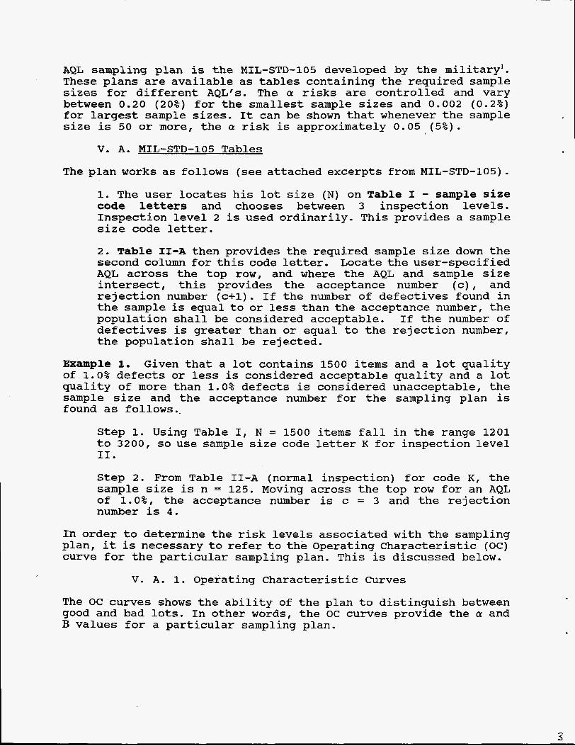
AQL sampling plan is the MIL-STD-105 developed by the military'. These plans are available as tables containing the required sample s i z e s f o r different AQL's. The a risks are controlled and vary between 0.20 (20%) for the smallest sample sizes and 0.002 (0.2%) for largest sample sizes, It can be shown that whenever the sample size is 50 or more, the a risk is approximately 0.05 (5%).

V. A. MIL-STD-105 Tables

The plan works as follows (see attached excerpts from MIL-STD-105).

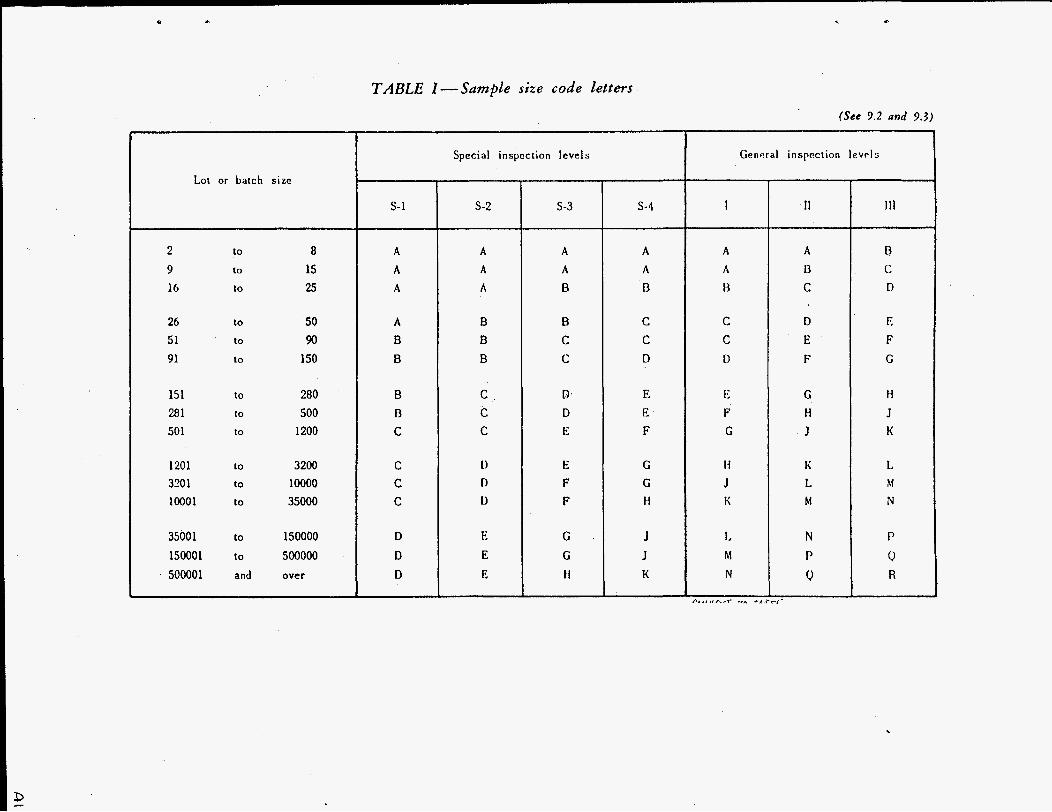
1. The user locates his lot size (N) on Table I - sample size code letters and chooses between 3 inspection levels. Inspection level 2 is used ordinarily. This provides a sample size code letter.

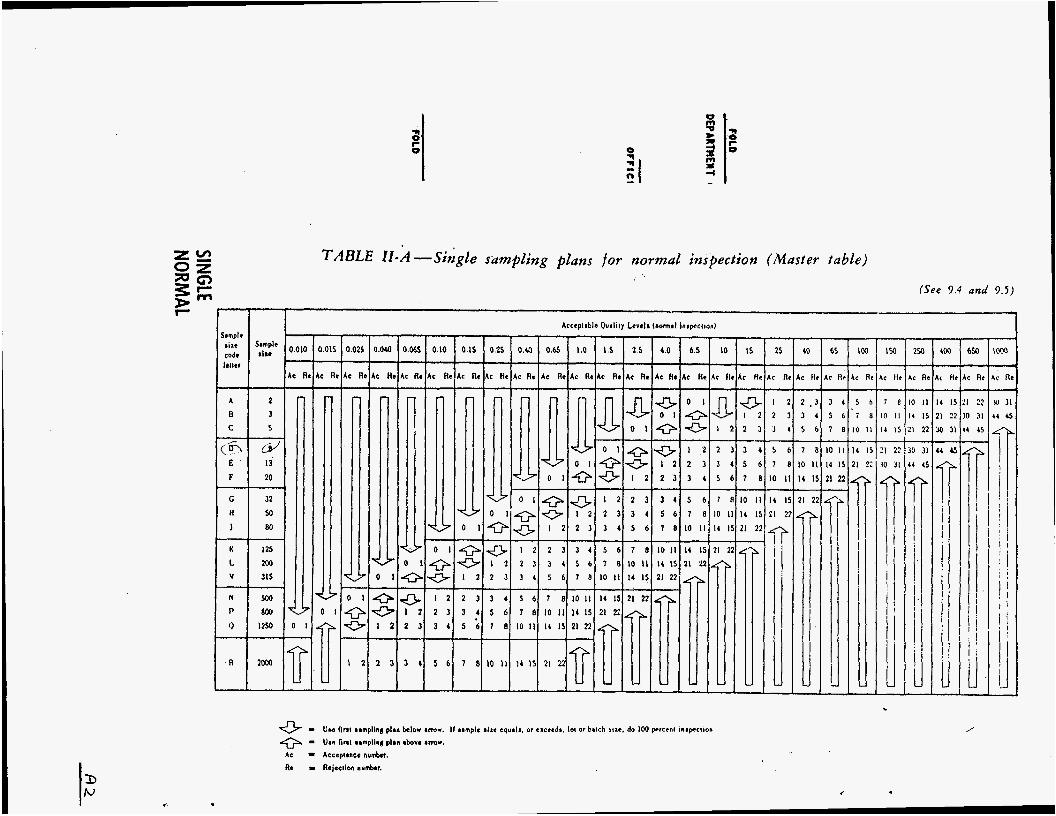
2. Table 11-A then provides the required sample size down the second column forthis code letter. Locate the user-specified AQL across the top row, and where the AQL and sample size intersect, this provides the acceptance number (c) , and rejection number (c+l). If the number of defectives found in the sample is equal to or less than the acceptance number, the population shall be considered acceptable. If the number of defectives is greater than or equal to the rejection number, the population shall be rejected.

Example 1. Given that a lot contains 1500 items and a lot quality of 1.0% defects or less is considered acceptable quality and a lot quality of more than 1.0% defects is considered unacceptable, the sample size and the acceptance number for the sampling plan is found as follows..

Step 1. Using Table I, N = 1500 items fall in the range 1201 to 3200, so use sample size code letter K for inspection level 11.

Step 2. From Table 11-A (normal inspection) for code K, the sample size is n = 125. Moving across the top row for an AQL of 1.0%: the acceptance number is c = 3 and the rejection number is 4 .

In order to determine the risk levels associated with the sampling plan, it is necessary to refer to the Operating Characteristic (OC) curve for the particular sampling plan. This is discussed below.

V. A, 1. Operating Characteristic Curves

The OC curves shows the ability of the plan to distinguish between good and bad lots. In other words, the OC curves provide the a and B values for a particular sampling plan.

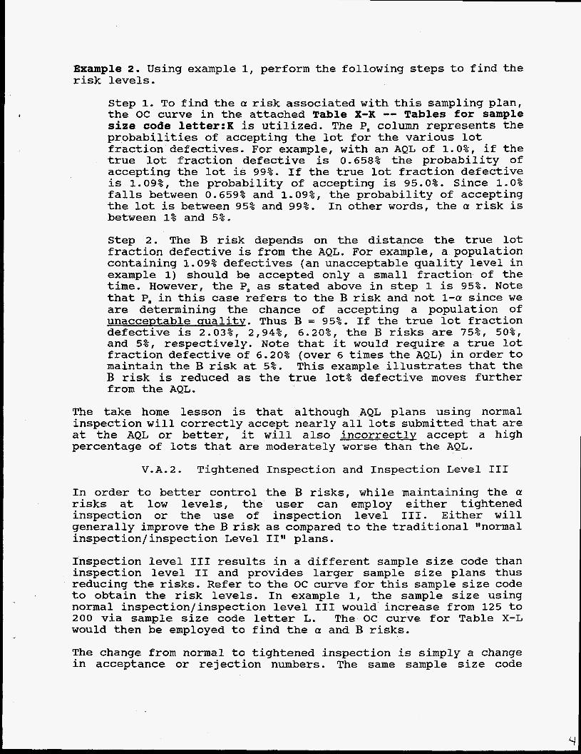
Example 2. Using example 1, perform the following steps to find the risk levels.

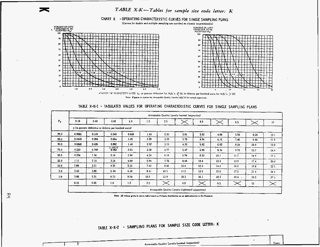
Step 1. To find the a risk associated with this sampling plan, the OC curve in the attached Table X-K -- Tables for sample size code 1etter:K is utilized. The Pa column represents the probabilities of accepting the lot for the various lot fraction defectives. For example, with an AQL of l.O%, if the true lot fraction defective is 0.658% the probability of accepting the lot is 99%. If the true lot fraction defective is 1.09%, the probability of accepting is 95.0%. Since 1.0% falls between 0.659% and l.O9%, the probability of accepting the lot is between 95% and 99%. In other words, the a! risk is between 1% and 5%.

Step 2. The B risk depends on the distance the true lot fraction defective is from t h e AQL. For example, a population containing 1.09% defectives (an unacceptable quality level in example 1) should be accepted only a small fraction of the time. However, the Pa as stated above in step 1 is 95%. Note that Pa in this case refers to the B risk and not 1-a! since we are determining the chance of accepting a population of unacceptable crualitv. Thus B = 95%. If the true lot fraction defective is 2.03%, 2,94%, 6.20%, the B risks are 75%, 50%, and 5%, respectively. Note that it would require a true lot fraction defective of 6.20% (over 6 times the AQL) in order to maintain the B risk at 5%. This example illustrates that the B risk is reduced as the true lot% defective moves further from the AQL.

The take home lesson is that although AQL plans using normal inspection will correctly accept nearly all lots submitted that are at the AQL or better, it will also incorrectly accept a high percentage of lots that are moderately worse than the AQL.

V.A.2. Tightened Inspection and Inspection Level I11

In order to better control the B risks, while maintaining the a! risks at low levels, the user can employ either tightened inspection or the use of inspection level 111. Either will generally improve the B risk as compared to the traditional Itnormal inspection/inspection Level 11" plans.

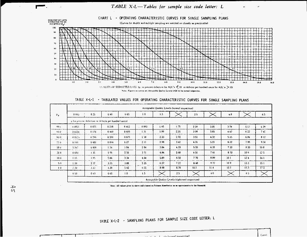
Inspection level I11 results in a different sample size code than inspection level I1 and provides larger sample size plans thus reducing the risks. Refer to the OC curve for this sample size code to obtain the risk levels. In example 1, the sample size using normal inspection/inspection level I11 would increase from 125 to 200 via sample size code letter L. The OC curve for Table X-L would then be employed to find the a! and B risks.

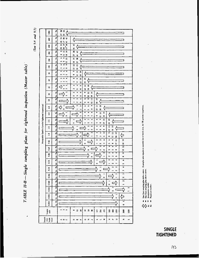
The change from normal to tightened inspection is simply a change in acceptance or rejection numbers. The same sample size code

4

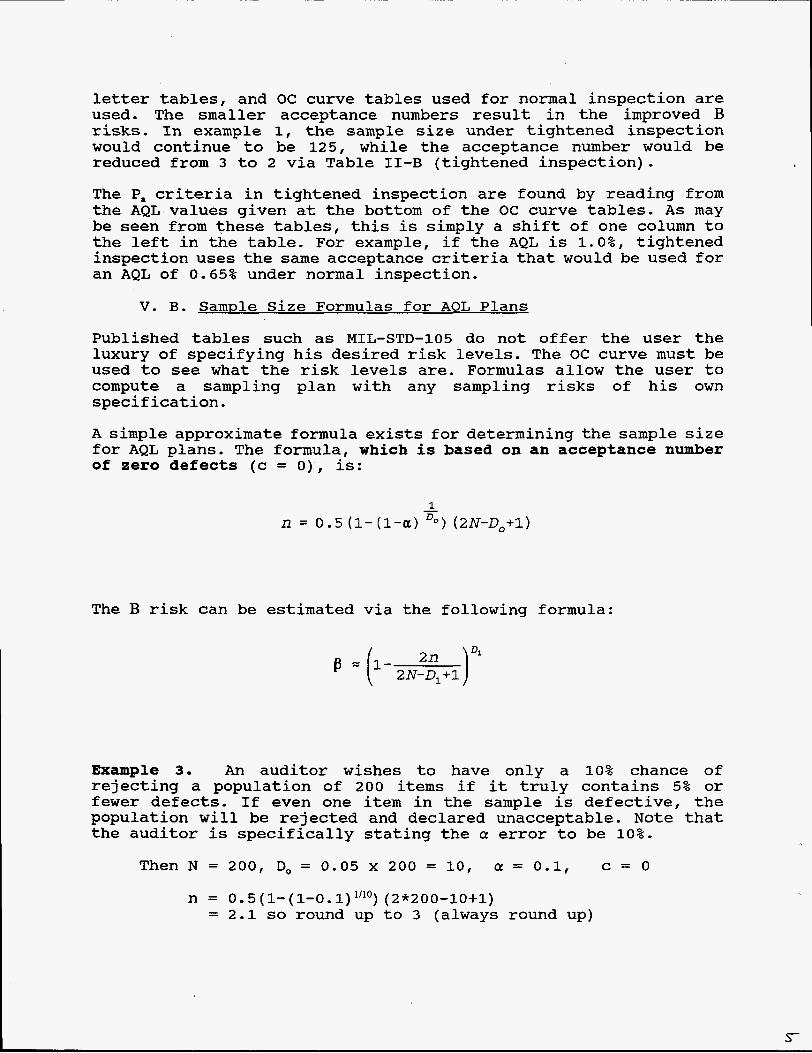
letter tables, and OC curve tables used for normal inspection are used. The smaller acceptance numbers result in the improved B risks. In example 1, the sample size under tightened inspection would continue to be 125, while the acceptance number would be reduced from 3 to 2 via Table 11-B (tightened inspection).

The Pa criteria in tightened inspection are found by reading from the AQL values given at the bottom of the OC curve tables. As may be seen from these tables, this is simply a shift of one column to the left in the table. For example, if the AQL is 1.0%, tightened inspection uses the same acceptance criteria that would be used for an AQL of 0.65% under normal inspection.

V. B. Sample Size Formulas for AOL Plans

Published tables such as MIL-STD-105 do not offer the user the luxury of specifying his desired risk levels. The OC curve must be used to see what the risk levels are. Formulas allow the user to compute a sampling plan with any sampling risks of his own specification.

A simple approximate formula exists for determiningthe sample size for AQL plans. The formula, which is based on an acceptance number of zero defects (c = 0) , is:

1 - R = O.S(l-(l-E) Do) (2N-DO+1)

The B risk can be estimated via the following formula:

Example 3. An auditor wishes to have only a 10% chance of rejecting a population of 200 items if it truly contains 5% or fewer defects. If even one item in the sample is defective, the population will be rejected and declared unacceptable. Note that the auditor is specifically stating the CY error to be 10%.

Then N = 200, Do = 0.05 x 200 = 10, CY = 0.1, c = 0

n = 0.5(1-(1-0.1)1’10) (2*200-10+1) = 2.1 so round up to 3 (always round up)

.

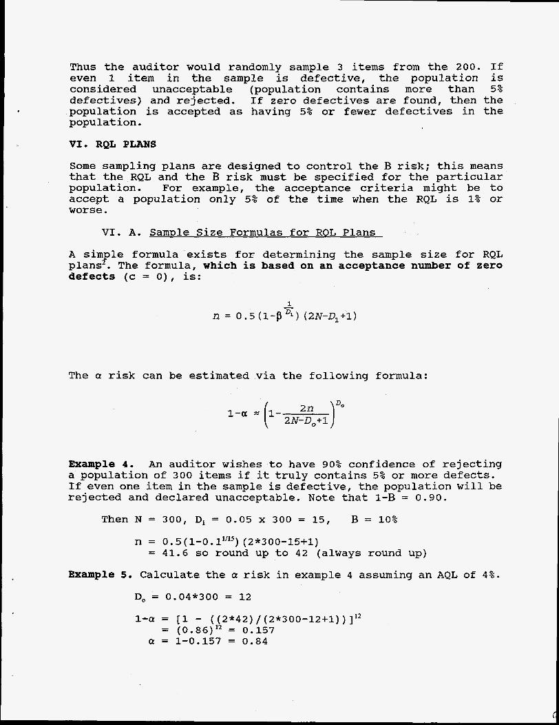
Thus the auditor would randomly sample 3 items from the 200, If even 1 item in the sample is defective, the population is considered unacceptable (population contains more than 5% defectives) and rejected. If zero defectives are found, then the population is accepted as having 5% or fewer defectives in the population.

VI. RQL PLANS

Some sampling plans are designed to control the B risk; this means that the RQL and the B risk must be specified for the particular population. For example, the acceptance criteria might be to accept a population only 5% of the time when the RQL is 1% or worse.

VI, A. SamDle Size Formulas for ROL Plans

A simple formula exists for determining the sample size for RQL plans2. The formula, which is based on an acceptance number of zero defects (c = O), is:

The a risk can be estimated via the following formula:

2 N- D,+1

Example 4. An auditor wishes to have 90% confidence of rejecting a population of 300 items if it truly contains 5% or more defects. If even one item in the sample is defective, the population will be rejected and declared unacceptable. Note that 1-B = 0.90.

Then N = 300, D, = 0.05 x 300 = 15, B = 10%

n = 0.5(1-0,11’15) (2*300-15+1) = 41.6 so round up to 42 (always round up)

Example 5 . Calculate the a risk in example 4 assuming an AQL of 4%.

Do = 0.04*300 = 12

1-a = [l - ((2*42)/(2*300-12+1)) 112 = (0 .86)12 = 0.157

CY = 1-0.157 = 0.84

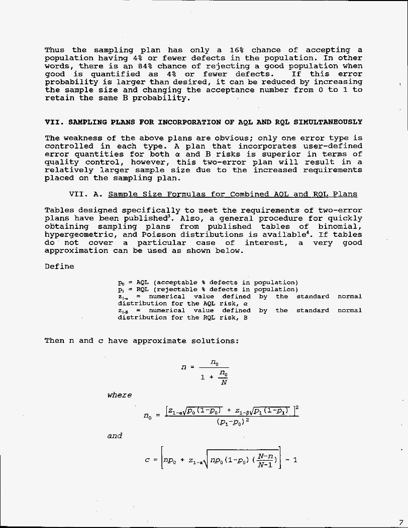
Thus the sampling plan has only a 16% chance of accepting a population having 4% or fewer defects in the population. In other words, there is an 84% chance of rejecting a good population when good is quantified as 4% or fewer defects. If this error probability is larger than desired, it can be reduced by increasing the sample size and changing the acceptance number from 0 to 1 to retain the same B probability.

VII. SAMPLING PLANS FOR INCORPORATION OF AQL AND RQL SIMULTANEOUSLY

The weakness of the above plans are obvious; only one error type is controlled in each type. A plan that incorporates user-defined error quantities for both a and B risks is superior in terms of quality control, however, this two-error plan will result in a relatively larger sample size due to the increased requirements placed on the sampling plan.

VII. A. Samrsle Size Formulas for Combined AOL and ROL Plans

Tables designed specifically to meet the requirements of two-error plans have been published3. Also, a general procedure for quickly obtaining sampling plans from published tables of binomial, hypergeometric, and Poisson distributions is available4. If tables do not cover a particular case of interest, a very good approximation can be used as shown below.

Define

po = AQL (acceptable % defects in population) pI = RQL (rejectable % defects in population) 2,- = numerical value defined by the standard normal distribution for the AQL risk, a =I-B - - numerical value defined by the standard normal distribution for the RQL risk, B

Then n and c have approximate solutions:

n0

n0 1 + - N

n =

where

and

r I 1

‘ I

7

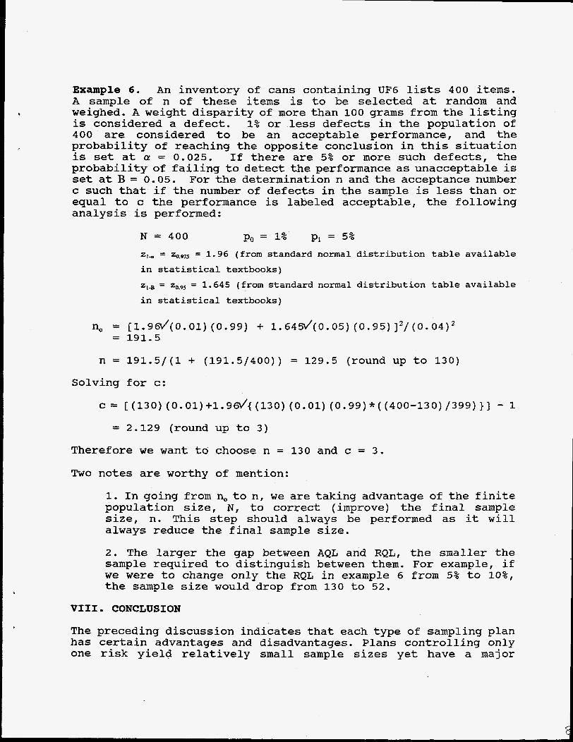
Example 6 . An inventory of cans containing UF6 lists 400 items. A sample of n of these items is to be selected at random and weighed. A weight disparity of more than 100 grams from the listing is considered a defect. 1% or less defects in the population of 400 are considered to be an acceptable performance, and the probability of reaching the opposite conclusion in this situation is set at a: = 0.025. If there are 5% or more such defects, the probability of failing to detect the performance as unacceptable is set at B = 0.05. For the determination n and the acceptance number c such that if the number of defects in the sample is less than or equal to c the performance is labeled acceptable, the following analysis is performed:

N = 400 po = 1% p, = 5%

zI* = zo.975 = 1.96 (from standard normal d is tr ibut ion tab le avai lable i n s t a t i s t i c a l textbooks) z ~ . ~ = z , , ~ ~ = 1.645 (from standard normal d is tr ibut ion tab le avai lable

i n s t a t i s t i c a l textbooks)

no = [1.96t/(0.01) (0.99) + 1.645/(0.05) (0.95)]2/(0.04)2 = 191.5

n = 191.5/(1 + (191.5/400)) = 129.5 (round up to 130)

Solving for c:

c = [ (130) (0.01)+1.9d((130) (0.01) (0.99)*( (400-130)/399)}] - 1 = 2.129 (round up to 3 )

Therefore we want to choose n = 130 and c = 3 .

Two notes are worthy of mention:

1. In going from no to n, we are taking advantage of the finite population size, N, to correct (improve) the final sample size, n. This step should always be performed as it will always reduce the final sample size.

2 . The larger the gap between AQL and RQL, the smaller the sample required to distinguish between them. For example, if we were to change only the RQL in example 6 from 5% to lo%, the sample size would drop from 130 to 52.

VIII. CONCLUSION

The preceding discussion indicates that each type of sampling plan has certain advantages and disadvantages. Plans controlling only one risk yield relatively small sample sizes yet have a major

disadvantage; the other risk is ignored and may be unacceptably large. Therefore, in using published tables, the user should always inspect the OC curve if the risks are not otherwise stated, to see that the plan accomplishes what is desired. Plans controlling both risks provide maximum desired protection for acceptance and rejection at the consequence of additional sampling. No one type of plan, therefore, can be recommended as being the best in all circumstances.

Any well-thought-out sampling plan must consider the acceptable quality levels and the risks associated with these levels. The auditor and auditee should be fully cognizant of the different types of risks of incorrect decisions embodied in the sampling plan and come to a common agreement regarding an appropriate sampling plan before beginning.

IX. REFERENCES

1. Department of Defense, Sampling Procedures and Tables f o r Inspection by Attributes, Military Standard 105E, Government Printing Office, Washington, D.C., May, 1989.

2. John Jaech, Statistical Methods in Nuclear Material Control, TID-26298, NTIS, Springfield, Virginia, 1973.

3 . Theodore S. Sherr, Attribute Sampling Inspection Procedure Based on the Hypergeometric Distribution, USAEC Report WASH-1210, Division of Nuclear Materials Security, May 1972. These tables provide solutions for 16 different combinations of a, B, AQL, and RQL . 4 . William, Guenther, "Use of the Binomial, Hypergeometric, and Poisson Tables to Obtain Sampling Planstt, Journal of Quality Technology, Vol. No. 2, April 1969.

DISTRIBUTION

Technical Information (2) Technical Library (2) Central Files (2) NMCtA (2) Laboratory QA and Statistical Services (5)

,

U f

TABLE I-Sample size code letters

(See 9.2 and 9.3)

Special inspection levels Cenvral inspection l e v ~ l s

Lot or batch size

-t C I3

D E F

C H J

K L M

N P P 0 0 R

I s- 1 s-2

A A A A A A

A B B B B B

C C C

L) 0 L)

D E D E D E

s-4 s-3

2 9 16

to

to to

8 15 25

A A B

C C D

E E F

C C H

I c,

26 51 91

to

to

to

50 90

150

151 281 501

to

to

to

280 500

1200

B B C

D, D E

E F C

H J K

E F F

H J K

L hl N

1201 3-301 10001

3200 10000 35000

C to to to

C C

L M N

35001 150001 500001

to 150000 to 500000 and over

C C ti

J J K

8 c 0 e

TABLE 11-A -Single sampling plans for normal inspection (Master table)

(See 9.4 and 9 , j J

Acerptabld Qual i ly Ltvdlr ( n o n i l inrpcciion)

h

I

1 2

a I UM lint i i m p l i n g plan below anow. I f i m p l t i i z c equals. or eiceedi. lot or batch stm. do 100 prccnt inaptction

+ - Uan nnt aamplin8 plan i b v r imr. l e Accopcaner numbrr. Re I Rcieclion number.

1

AC R l

10 I I I 4 IS 2 1 22

:I 22 IO 31

30 31 44 45

,

I

6% - E Re

I ?? 3 31

t 45 - r i . I

- Li

i ! i : i

1

c

Y i Q.

I Ep 4 rs

- I ;- E“3 I

c - a - 0 Y ” Y

* .4

.I .-

SINGLE TI WTENfD

(33

PiXCEYT OC LOIS , I. XPECTED fo BE ACCEPTED tP.1

TABLE X-K-Tables for sample size code letter: K

CHART K - OPERATING CHARACTERISTIC CURVES FOR SINGLE SAMPLING P IANS (Curves for double m d multiple simplin8 are mmtchnl am closely as practicable)

1.0 2 0 3 0 4 0 5.0 611 7 0

la,

PO

80

IO

m

Y)

40

SO

10

10

0

TABLE X-K-1 - TABULATED VALUES FOR OPERATING CHARACTERISTIC CURVES FOR SINGLE SAMPLING PLANS

Acccpiablc Vuality Lcveli (normal inspection)

pm 0.10 0.40 0.65 1 .o I .5 2.5 1x1 4.0 6.5 IO

p (in percent defective or defects per hundred uniisJ

99.0 0.0081 0. I I9 0.349 0.658 I .43 2.33 2.81 3.82 4.88 5.90 8.28 1p I

75.0 0.230 0.769 '$g

9s.u 0.0410 0.284 0.654 I .09 2.09 3.19 3.76 4.94 6.15 7.40 9.95 11.9

90.0 0.0840 0.426 0.882 1.40 2.52 3.73 4.35 5.62 6.92 8.24 10.9 13.0 .--

2.03 3.38 4.77 5.47 6.90 8.34 9 79 12.1 14.9

25.0 1 .11 2.15 3.14 4.09 5.94 7.75 8.64 10.4 12 2 13.9 17 4 20 0

10.0 1 .a ~ 3.11 4.26 5.35 7.42 9.42 10.4 12.3 14.2 16. I 19.8 22 5

50.0 0.554 1.34 2.14 2.94 4.54 6.14 6.94 8.53 10. I 11.1 I4 9 17.3

- 5.0 2.40 3.80 5.04 6.20 8.4i 10 5 I1.5 13.6 15.6 17.5 21.4 24 2

1.0 3.68 5.31 6.73 8.04 10.5 12 fl 18.3 16.1 18.3 20.4 . 24.5 21 5 -

, I .o , 1 .5 2.5 > < \ 4.0 X 6.5 x 10 x 0.15 C.65 - ~~

Acceptable Quality Levels (tiKhtened inspection) J

N O W All 1d.r dn. I. &pn Id. b r u d OD Pol- dl.ulkil.. u - 9plod.vlom ID LL. 8hul.l.

TABLE X-K-2 - SAMPLING PLANS FOR SAMPLE SIZE CODE LETTER: K'

PERCENTOFLOTS EXPECTED TO HE

ACCWTEO Ira)

TABLE X-L-Tables for sample size code letter: L

CHART L - OPERATING CHARACTERISTIC CURVES FOR SINGLE SAMPLING PLANS (Cunes for double and multiple sampling are matched a 3 closely as pncocable)

100

w

80

70

M

51'

( ( 8

M

20

I U

n

TABLE X-L - I - TABULATED VALUES FOR OPERATING CHARACTERISTIC CURVES FOR SINGLE SAMPLING PLANS

1 1 Acceptable Vudtly Levels (nonnal mspcctton) 1

t- 25 0

5 0

I I O

--.--I 35 I 96 2 56 3 71 4 84 540 6 51 7 61 8 70 10 9 I ? 5

1 9 5 2 6 6 3 30 4 6 4 5 89 650 7 70 889 IO I 12 4 14 I

I 50 2 37 3 15 3 88 5 26 6 57 7 22 848 9 7: I O 9 13 3 IS 1

2 30 J J? 4 2 0 5 02 (r 55 8 0 0 8 70 10 I I I 4 12 7 I5 3 17 2

^__I_- _ _ _ _ - -

0 IO 0 40 0 bs I O I S x 2 5 X 4 0 x 6 5 X

TABLE X-L-2 - SAMPLING PLANS FOR SAMPLE S I Z E CODE LRTER: L