A comparative study on the path length performance of maze ......A~stract-Maze-searching algorithms first appeared in graph theory and, more recently, have been studied in works on

IEEE TRANSACTIONS ON ROBOTICS AND AUTOMATION, VOL. I , NO. 1 , FEBRUARY 1991

~

57

A Comparative Study on the Path Length Performance of Maze-Searching and

Robot Motion Planning Algorithms

Vladimir J. Lumelsky , Senior Member, IEEE

A~stract-Maze-searching algorithms first appeared in graph theory and, more recently, have been studied in works on computational complexity. Although the formulation of the maze-search problem shows a clear relation to robotics, there have been no consistent attempts to connect these two fields. In this paper, a number of existing maze- searching and robot motion planning algorithms are studied from the standpoint of a single performance criterion. Our main motivation is to build a framework for selecting basic planning algorithms for au- tonomous vehicles and robot arm manipulators that operate in an environment filled with unknown obstacles of arbitrary shapes. In choosing an appropriate criterion, it is noted that besides convergence, minimizing the length of generated paths is a single major consideration in planning algorithms. In addition, since no complete information is ever available, optimal solutions are ruled out. Accordingly, the performance criterion is defined in terms of the upper bound on the length of generated paths as a function of the length of maze walls. The comparison shows that the special structure of graphs that correspond to planar environments with obstacles actually allows one to exceed the efficiency of general maze-searching algorithms.

I. INTRODUCTION E are considering the problem of path planning for a point W automation (a robot) operating in a planar scene with

obstacles. Only approaches that guarantee convergence (non- heuristic approaches) will be considered. In the accepted model (referred to in the literature as the model with incomplete information, motion planning with uncertainty, or sensor-based robot motion planning), the objective of the automaton is, starting in the initial position S , to generate a collision-free path to a predefined target point T or to prove that T cannot be reached. The automaton has no knowledge about the geometry and positions of the obstacles. The automaton has sensors that allow it to detect an obstacle once it approaches one and to walk along the obstacle boundary. Each obstacle is of finite perimeter and of arbitrary shape and presents a simple closed curve. In general, the environment (maze) is infinite. Any disk of finite radius would intersect a finite number of obstacles. Similarly, a straight-line segment of finite length intersects obstacles in a finite number of points. Obstacles do not touch each other. Depending on the specific algorithm, some additional input information may be assumed. By its very nature, the problem calls for on-line (real-time) algorithms. Since these algorithms operate with limited information available to the automaton at a

Manuscript received February 9, 1989. This work was supported by the National Science Foundation under Grants DMC-87 12357 and IN-8805943 and by a grant from Philips Corporation.

The author is with the Department of Electrical Engineering, Yale Univer- sity, New Haven, CT 06520.

IEEE Log Number 9040305.

given moment, they can be called local algorithms. In general, local algorithms can be expected to be quite different and not as efficient as global algorithms.

As formulated, the problem of robot motion planning is quite similar to the maze-search problem, which was first considered in graph theory and, more recently, in works on computational complexity. In spite of this similarity, very little attention has been paid to comparative studies on maze-searching algorithms and robot motion planning with incomplete information. In those rare works where maze searching is tied to robot motion planning, e.g., [4], no attempts have been made to assess the algorithm performance quantitatively. This is in contrast with extensive literature that ties motion planning and graph search problems within the context of the model with complete information [l].

The importance of comparing the performance of various algorithms of motion planning with incomplete information lies in the following facts:

Besides convergence, minimizing the length of generated paths is a single major consideration in robot motion planning systems. Because of the lack of complete information, optimal solutions are ruled out. As will be shown below, different algorithms exhibit significant variation in their path length performance. The importance of such algorithms is underscored by the fact that they can be used, with proper modifications, for sensor-based collision-free motion planning of industrial robot arm manipulators [6].

The latter connection is due to the fact that for some two- and three-dimensional arm manipulators, the motion planning problem can be reduced to that of a point automaton operating in a certain two-dimensional manifold, with the workspace obstacles forming an unknown maze in the manifold. As a simple example, any two- or three-dimensional two-link manipulator with revolute and/or sliding joints can be represented by a point on the surface of a common torus or of a subset of such torus.

’ The model with incomplete information is distinct from another formulation of the robot motion planning problem, which is often referred to as the model with complete information, in which full information about the geometry and positions of the robot and obstacles in the scene is given. All the surfaces of the obstacles and the robot are then assumed to be algebraic, e.g., presenting polygons. Consequently, path planning becomes a one-time, off-line computational operation, which calls for global algorithms. A survey of work in this area can be found in [I].

1042-296X/91/02OO-OO57$01 .OO 0 1991 IEEE

Authorized licensed use limited to: University of Wollongong. Downloaded on September 28, 2009 at 11:45 from IEEE Xplore. Restrictions apply.

58 IEEE TRANSACTIONS ON ROBOTICS AND AUTOMATION, VOL. 7. NO. I , FEBRUARY 1991

One difficulty with comparing the performance of different algorithms is that, for some motion planning algorithms, their performance is either not known or has been presented in terms of different criteria. This paper attempts to study the performance of various algorithms within a framework of a single performance criterion tied to the length of generated paths.

There are two different versions of the maze-search problem that one finds in literature. In one version, which is also considered in this paper, the automaton is required to escape from or find a specific point inside or outside a planar continu- ous maze. In another version, which is more typical for the work in computational complexity, the maze is assumed to be divided into finite cells, and the automaton must eventually visit every reachable cell. The complexity of the latter problem has been investigated in a number of works (see [2] and [3] and references therein). When the goal is to escape from the maze, the maze is assumed to be of finite size.’ When the goal is to find a prespecified location, the maze may be infinite.

As defined in graph theory, a maze presents a finite collection of enclosed narrow corridors interconnected in different ways with clearly defined intersections. A maze can easily be reduced to a graph, where maze corridors become the edges and their intersections-the vertices of the graph. Note that this formulation carries an implicit assumption that the point automaton follows both walls of the corridor simultaneously. In general, this may or may not be possible. For example, obstacles in the robot environment may be of irregular shapes and far apart so that the robot would follow only one “wall” at a time; the environment itself can be finite or infinite. Furthermore, the obstacles may be disconnected, which renders some popular maze-searching strategies (such as, “At a junction, always take the passageway on the extreme right”[l2]) inadequate. As a result, the maze-to-graph reduction is not simple and, more importantly, not unique.

To assure consistency in comparing various approaches to the maze-search problem, we utilize instead the above model of the environment used in robotics that presents a certain generaliza- tion of the idea of maze and can be called a “general maze.” A general maze does not necessarily have clearly defined corridors and intersections. In the special case when the maze is built out of narrow corridors, the automaton will be assumed to follow one wall at the time, which means that, on the graph, the corridor will correspond to two edges, both connecting the same two vertices.

In the following sections, a single framework for relating different approaches to motion planning with incomplete information is introduced (Section 11,) and five different motion planning algorithms are evaluated in terms of their path length performance. Out of these, two maze-searching algorithms are reviewed in Section 111, and two robot motion planning algorithms are reviewed in Section IV. This is followed, in Section V, by still another maze-searching strategy, called the Pledge algorithm [4], whose performance is derived anew. Section VI contains a summary on the performance of the five algorithms. Finally, in Section VII, the performance of those algorithms is compared in an example with the same single maze.

* Imagine, for example, that the automaton is a mouse looking for food located inside or outside the maze-this is the context of the MicroMouse competition of mechanical mice conducted annually in the United States (under the auspices of the Institute of Electrical and Electronics Engineers) and also in England and Japan.

tT :d7

12;

1

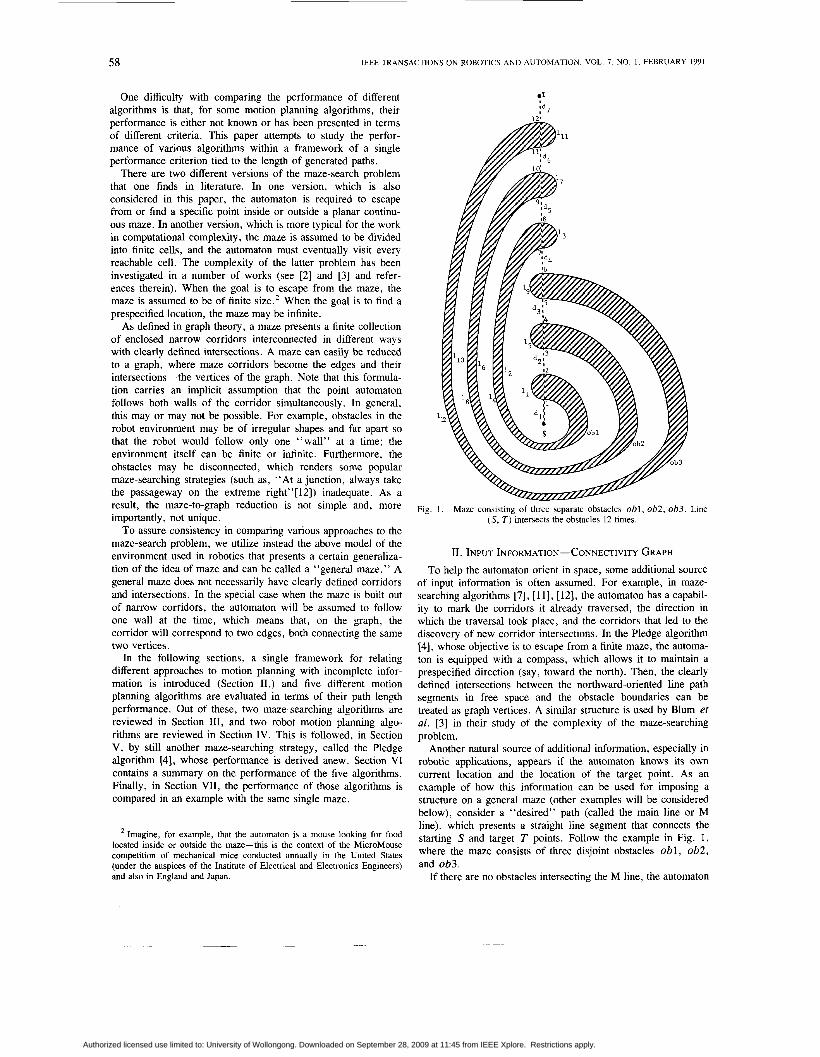
Fig. 1. Maze consisting of three separate obstacles obl, ob2, ob3. Line ( S , T ) intersects the obstacles 12 times.

11. INPUT INFORMATION- CONNECTIVITY GRAPH To help the automaton orient in space, some additional source

of input information is often assumed. For example, in maze- searching algorithms [7], [ 1 11, [ 121, the automaton has a capability to mark the corridors it already traversed, the direction in which the traversal took place, and the corridors that led to the discovery of new corridor intersections. In the Pledge algorithm [4], whose objective is to escape from a finite maze, the automaton is equipped with a compass, which allows it to maintain a prespecified direction (say, toward the north). Then, the clearly defined intersections between the northward-oriented line path segments in free space and the obstacle boundaries can be treated as graph vertices. A similar structure is used by Blum et al. [3] in their study of the complexity of the maze-searching problem.

Another natural source of additional information, especially in robotic applications, appears if the automaton knows its own current location and the location of the target point. As an example of how this information can be used for imposing a structure on a general maze (other examples will be considered below), consider a “desired” path (called the main line or M line), which presents a straight line segment that connects the starting S and target T points. Follow the example in Fig. I , where the maze consists of three disjoint obstacles ob l , ob2, and ob3.

If there are no obstacles intersecting the M line, the automaton


LUMELSKY: PATH LENGTH PERFORMANCE OF MOTION PLANNING ALGORITHMS 59

IS

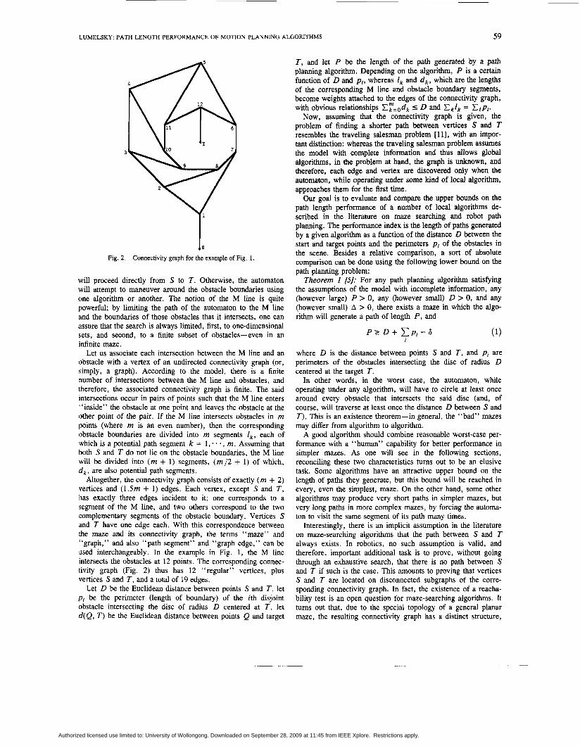
Fig. 2. Connectivity graph for the example of Fig. 1 .

will proceed directly from S to T . Otherwise, the automaton will attempt to maneuver around the obstacle boundaries using one algorithm or another. The notion of the M line is quite powerful; by limiting the path of the automaton to the M line and the boundaries of those obstacles that it intersects, one can assure that the search is always limited, first, to one-dimensional sets, and second, to a finite subset of obstacles-even in an infinite maze.

Let us associate each intersection between the M line and an obstacle with a vertex of an undirected connectivity graph (or, simply, a graph). According to the model, there is a finite number of intersections between the M line and obstacles, and therefore, the associated connectivity graph is finite. The said intersections occur in pairs of points such that the M line enters “inside” the obstacle at one point and leaves the obstacle at the other point of the pair. If the M line intersects obstacles in m points (where m is an even number), then the corresponding obstacle boundaries are divided into m segments I,, each of which is a potential path segment k = 1, * * * , rn. Assuming that both S and T do not lie on the obstacle boundaries, the M line will be divided into (m + 1) segments, (m /2 + 1) of which, d,, are also potential path segments.

Altogether, the connectivity graph consists of exactly (m + 2) vertices and (1.5m + 1) edges. Each vertex, except S and T , has exactly three edges incident to it; one corresponds to a segment of the M line, and two others correspond to the two complementary segments of the obstacle boundary. Vertices S and T have one edge each. With this correspondence between the maze and its connectivity graph, the terms “maze” and “graph,” and also “path segment” and “graph edge,” can be used interchangeably. In the example in Fig. 1, the M line intersects the obstacles at 12 points. The corresponding connectivity graph (Fig. 2) thus has 12 “regular” vertices, plus vertices S and T , and a total of 19 edges.

Let D be the Euclidean distance between points S and T , let pi be the perimeter (length of boundary) of the ith disjoint obstacle intersecting the disc of radius D centered at T , let d(Q, T ) be the Euclidean distance between points Q and target

T , and let P be the length of the path generated by a path planning algorithm. Depending on the algorithm, P is a certain function of D and pi, whereas I, and dk, which are the lengths of the corresponding M line and obstacle boundary segments, become weights attached to the edges of the connectivity graph, with obvious relationships CF=odk s D and C k l k = X i p i .

Now, assuming that the connectivity graph is given, the problem of finding a shorter path between vertices S and T resembles the traveling salesman problem [ 111, with an important distinction: whereas the traveling salesman problem assumes the model with complete information and thus allows global algorithms, in the problem at hand, the graph is unknown, and therefore, each edge and vertex are discovered only when the automaton, while operating under some kind of local algorithm, approaches them for the first time.

Our goal is to evaluate and compare the upper bounds on the path length performance of a number of local algorithms described in the literature on maze searching and robot path planning. The performance index is the length of paths generated by a given algorithm as a function of the distance D between the start and target points and the perimeters p i of the obstacles in the scene. Besides a relative comparison, a sort of absolute comparison can be done using the following lower bound on the path planning problem:

Theorem 1 [5]: For any path planning algorithm satisfying the assumptions of the model with incomplete information, any (however large) P > 0, any (however small) D > 0, and any (however small) A > 0, there exists a maze in which the algorithm will generate a path of length P , and

P ? D + C p i - 6 (1) i

where D is the distance between points S and T , and p i are perimeters of the obstacles intersecting the disc of radius D centered at the target T .

In other words, in the worst case, the automaton, while operating under any algorithm, will have to circle at least once around every obstacle that intersects the said disc (and, of course, will traverse at least once the distance D between S and T ) . This is an existence theorem-in general, the “bad” mazes may differ from algorithm to algorithm.

A good algorithm should combine reasonable worst-case performance with a “human” capability for better performance in simpler mazes. As one will see in the following sections, reconciling these two characteristics turns out to be an elusive task. Some algorithms have an attractive upper bound on the length of paths they generate, but this bound will be reached in every, even the simplest, maze. On the other hand, some other algorithms may produce very short paths in simpler mazes, but very long paths in more complex mazes, by forcing the automaton to visit the same segment of its path many times.

Interestingly, there is an implicit assumption in the literature on maze-searching algorithms that the path between S and T always exists. In robotics, no such assumption is valid, and therefore, important additional task is to prove, without going through an exhaustive search, that there is no path between S and T if such is the case. This amounts to proving that vertices S and T are located on disconnected subgraphs of the corresponding connectivity graph. In fact, the existence of a reachability test is an open question for maze-searching algorithms. It turns out that, due to the special topology of a general planar maze, the resulting connectivity graph has a distinct structure,


60 IEEE TRANSACTIONS ON ROBOTICS AND AUTOMATION, VOL. 7, NO. 1 , FEBRUARY 1991

which allows one to develop a target reachability test based on an appropriate necessary and sufficient condition (see Section IV) *

111. MAZE-SEARCHING ALGORITHMS In addition to the assumptions of the model with incomplete

information described in the Introduction, assume that the automaton is capable of identifying the corridors it already traversed, the direction in which the traversal took place, and the corridors that led to the discovery of the corridor intersections. In the case of a general infinite or finite maze, the automaton will also need some additional orientation means in order to reduce the maze to a finite connectivity graph. For specificity, assume that the automaton knows its own current coordinates and those of the target, and the graph is based on the M line as described in Section 11.

Since in the worst case the automaton will have to traverse every edge of the graph at least once in order to reach its target, the problem of generating shorter paths is closely related to that of generating an Eulerian chain in the graph-that is, such a path between the start and target vertices where each edge on the path is traversed exactly once. The necessary and sufficient condition for such a path to exist was given by Euler based on the famous Konigsberg bridge problem that he formulated in 1736; his theorem says that for the Eulerian chain to exist, the number of edges incident to every vertex of the graph must be even; if the start and target vertices are distinct, each of them must have an odd number of incident edges [ l l ] . Such graphs are called Euler graphs. Interestingly, there exist a number of global algorithms, but there are no local algorithms for finding Eulerian chains [ 121.

One of the main driving forces behind Euler’s work on the Konigsberg bridge problem was his interest in the topological characteristics of closed curves; in fact, the problem became the beginning of the field of topology. All the subsequent studies of the maze-search problem were tied to the graph theory alone and did not take into account the topologies that generated the graphs. One of the first systematic local maze-searching algorithms, described by Wiener in 1873 [ l l ] , reduced the problem to a rather inefficient exhaustive search, in which each edge would be traversed many times but not less than twice. Two other algorithms, by Tremaux and Tarry, traverse every edge exactly twice [ l l ] . Since both are quite similar, we consider only the latter.

Tarry’s Algorithm: For a given maze (graph), when the automaton arrives at a vertex U , the following input information is assumed: 1) the subset of those edges incident to U that the automaton used previously to leave U , i.e., those edges that were traversed in the direction pointing away from U ; 2) the entrance edge via which the automaton first arrived at U. The procedure is very simple:

Upon arrival at U , continue via an edge ( U , U?, which was not yet traversed in the direction of U to U’. Choose the entrance edge as a last resort.

1)

2) Tarry’s theorem states that under this algorithm, assuming the

start and target vertices are distinct and there is a path between them, the target vertex is guaranteed to be reached, and every edge will be traversed exactly twice, once in each direction, with the exception of the edges incident to the start and target vertices, which will be traversed once each. Using our terminology and ignoring the lengths of the edges incident to S and T (in the worst case, they will be zeros), the upper bound on the

length of paths generated by the algorithm can be presented as follows:

Theorem 2: For any finite maze, Tarry’s algorithm will generate a path of length P such that

P = 2 D + 2 c p i (2) I

where pi are the perimeters of the obstacles in the maze. Fraenkel’s Algorithm: The version of Tarry’s algorithm

suggested by Fraenkel [7] is more economical; the algorithm never traverses each edge of the path more than twice, and if “lucky,” some ( or even all) edges may be traversed just once. In addition to the input information available in Tarry’s algorithm, Fraenkel’s algorithm makes use of a counter, which at the start vertex is set to zero. The algorithm operates as follows:

1) Whenever you arrive at a vertex not visited before, increase the counter by 1 .

2) If you arrive at a vertex U such that before entering it there was at least one edge incident to it that was not traversed before and on arrival at U there remains at most one such edge, decrease the counter by 1 . As long as the counter is positive, the tour is conducted according to Tarry’s algorithm, except whenever possible, an edge not traversed before is preferred to an edge already traversed before.

4) As soon as the counter contains zero, leave all edges via their entrance edges.

The accompanying theorem states (it is derived for the case when the start and target vertices coincide) that, under this algorithm, the target vertex, if reachable, is guaranteed to be reached, and every edge will be traversed at least once but never more than twice, once in each direction. Using our terminology, the upper bound on the length of paths generated by the algorithm can be presented as follows:

Theorem 3: For any finite maze, Fraenkel’s algorithm will generate a path of length P such that

3)

P I 2 0 + 2 c p i i

(3)

where pi are the perimeters of the obstacles in the maze. In other words, the worst-case estimates of the length of

generated paths for Tarry’s and Fraenkel’s algorithms are identical. However, the performance of Fraenkel’s algorithm can be better, and never worse, than that of Tarry’s algorithm. For example, if the graph presents a Euler graph, Fraenkel’s automaton, if “lucky,” may traverse each edge only once. Note that our connectivity graph is not a Euler graph (each vertex has an odd number of edges incident to it), but it could be transformed into a Euler graph, for example, by duplicating all the M line segments between obstacles, except those incident to S and T .

Each of the two algorithms above is based solely on the graph-theoretical considerations and is not trying to exploit the topology of the mazes that produce the connectivity graphs. For example, the fact that each obstacle boundary must represent a closed curve is not taken into account. Algorithms that exploit the maze topology are considered in the next section.

IV. ROBOT MOTION PLANNING ALGORITHMS In addition to the assumptions of the model with incomplete

information described in the Introduction, assume that the automaton knows its own coordinates and those of the target at all times. The main idea of the two algorithms described below



comes from the following simple topological facts: 1) Although the planar regions of the free space between obstacles present two-dimensional sets, the fact that any such set is compact suggests that exploring one-dimensional sets, such as obstacle boundaries, should be sufficient for solving the problem at hand; 2) there are only two directions for following a simple closed curve (an obstacle boundary) -clockwise or counterclockwise; 3) if one starts walking in one direction along a simple closed curve, one will eventually come back to the starting point; 4) in the vicinity of a given point lying on the curve, if one tries both directions of following the curve, one exhausts all the possibili- ties for local exploration of the curve. These facts are corollaries to the Jordan curve theorem:

Jordan Curve Theorem [8]: Any closed curve homeomor- phic to a circle drawn around and in the vicinity of a given point on an orientable surface divides the surface into two separate domains, for which the curve is their common boundary.

In our case, the closed curve presents the boundary of a given obstacle, and the two domains are the obstacles and the free space, respectively. The vertices of the connectivity graph on which algorithm operates represent intersections between some straight line(s) aiming toward the target T and the obstacles within the disc of radius D centered at T . The automaton is said to define a hit point H on the obstacle when, while moving along a straight line toward T , it contacts the obstacle at point H. It defines a leave point L on the obstacle when it leaves the obstacle at point L in order to continue its straight line walk toward T . Touching an obstacle tangentially does not count-the automaton simply continues its straight line walk toward T . Thus, no point can be defined as both an H and an L point.

Algorithm Bugl [5]: In this procedure, when encountering an ith obstacle, the automaton defines a hit point Hi, i = 1,2, * . When leaving the ith obstacle, to continue its travel toward T , the automaton defines a leave point L,; initially, i = 1; L o = S. The procedure uses three registers R , , R , , R , , to store intermediate information; all three are reset to zero when a new hit point Hi is defined. Specifically, R , is used to store the coordinates of the current point Q, of the minimum distance between the obstacle boundary and T ; R , integrates the length of the obstacle boundary starting at Hi; R , integrates the length of the obstacle boundary starting at Q,. The test for target reachability mentioned in Step 3 of the procedure is formulated later in this section. The procedure consists of the following steps:

From point L i - , , move toward the target T along a straight line until one of the following occurs: a) T is reached. The procedure stops. b) An obstacle is encountered, and a hit point Hi is

defined. Go to Step 2. Turn left and follow the obstacle boundary. If T is reached, stop. Otherwise, after having traversed the whole boundary and having returned to Hi , define a new leave point Li = Q,. Go to Step 3. Based on the contents of registers R , and R, , determine the shorter way along the boundary to L; , and use it to reach L;. Apply the test for target reachability. If T is not reachable, the procedure stops. Otherwise, set i = i + 1 and go to Step 1.

It can be shown that the following necessary and sufficient condition holds: If the automaton, after having arrived at point L i , discovers that the straight line ( L , , T ) crosses some obstacle at Doint L j . then T is not reachable-either point S or T is

trapped inside the ith obstacle. Based on that , the test for target reachability used in Step 3 of the procedure is formulated as follows.

Test fo r Target Reachability, Bugl Algorithm: If, after having defined a point L , the automaton discovers that the straight line segment ( L , T ) crosses the obstacle at point L , then target T is not reachable.

Under this algorithm, the vertices of the connectivity graph are produced by the intersections between the straight line segments ( L i , T ) and those obstacles that intersect the disc of radius D centered at T . Once the automaton leaves an obstacle, it never returns to it again. The following theorem gives an upper bound on the length of paths produced by the algorithm.

Theorem 4 [5]: The length P of a path generated by the Bugl Algorithm is bounded by

P S D + 1 . 5 . cpi (4) i

where pi refer to the perimeters of obstacles that intersect the disc of radius D centered at T .

Algorithm Bug2 [5]: The connectivity graph in this procedure is based on the M line, as explained in Section 11. The hit and leave points are those of intersections between the M line and the obstacles. Because the automaton may define more than one hit or leave point on the same,obstacle, the numbering changes; the superscript j in the H J or L J indicates the j th Occurrence of the respective point on the same or other obstacle. Initially, j = 1; Lo = S. The test for target reachability built into Steps 2(b) and (c) of the procedure is explained later in this section. The algorithm consists of the following steps:

From point L J - ' , move along the M line until one of the following occurs: a) T is reached. The procedure stops. b) An obstacle is encountered, and a hit point H J is

defined. Go to Step 2. 2) Turn left and follow the obstacle boundary until one of

the following occurs: a) T is reached. The procedure stops. b) The M line is met at a point Q such that the distance

d ( Q , T ) c d ( H J , T ) , and the line (Q, T ) does not cross the current obstacle at point Q. Define the leave point LJ = Q . Set j = j + 1. Go to Step 1.

c) The automaton returns to H J and thus completes a closed curve without having defined the next hit point f f J + ' . The target is trapped and cannot be reached. The procedure stops.

1)

Under this procedure, a local cycle is created if the automaton passes some point(s) of its path more than once.

Test for Target Reachability, Bug2 Algorithm: If, on the pth local cycle, p = 0, 1, a , after having defined a point H J , the automaton returns to this point before it defines at least the first two out of the possible set of points LJ, H J + ' , LJ+', . a , H k , it means that the automaton has been trapped, and hence, target T is not reachable.

Let n, be the number of intersections between the M line and the ith obstacle; thus n, is a characteristic of the set (scene, start, target) and not of the specific algorithm. Obviously, for any convex obstacle n, = 2. Then, the following theorem gives an upper bound on the length of paths produced by the algorithm.

Theorem 5 f5/: The length of a path generated by the Bug2



I I

ob2 ( 5 )

niPi P I : D + C -

i 2

where p i refer to the perimeters of obstacles that intersect the disc of radius D centered at T.

In other words, the worst-case performance of the Bug2 Algorithm is not bounded; it may generate any (finite) number of local cycles. It can be shown, however [ 5 ] , that in the case of convex obstacles and in many cases on nonconvex obstacles, the performance of Bug2 is very good; namely, the worst-case upper bound approaches the lower bound (1)

and, on average, the performance is better than the lower bound (1)

P 5 D + 0.5 * c p i . (7) i

V. PATH LENGTH PERFORMANCE OF PLEDGE ALGORITHM

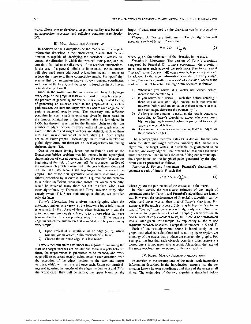
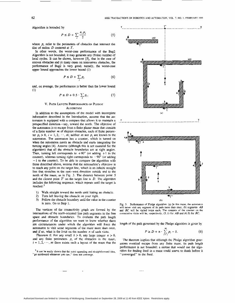
In addition to the assumptions of the model with incomplete information described in the Introduction, assume that the automaton is equipped with a compass that allows it to maintain a prespecified direction-say , toward the north. The objective of the automaton is to escape from a finite planar maze that consists of a finite number m of disjoint obstacles, each of finite perimeter p i > 0, i = 1,2; .* , m; neither m nor p i are known to the automaton. The automaton has a counter, which is turned on when the automaton meets an obstacle and starts integrating the turning angles [4]. Assume (although this is not essential for the algorithm) that all the obstacle boundaries are at right angles. Then, turning left corresponds to +90” (or adding + 1 to the counter), whereas turning right corresponds to - 90” (or adding - 1 to the counter). To be able to compare the algorithm with those described above, assume that the automation’s objective is to reach any point on the target line, which is an infinite straight line that stretches in the east-west direction outside and to the north of the maze, as in Fig. 3. The distance between point S and the closest point T‘ on the target line is D . The algorithm includes the following sequence, which repeats until the target is r e a ~ h e d . ~

1) Walk straight toward the north until hitting an obstacle. 2) Turn left leaving the obstacle on your right. 3) Follow the obstacle boundary until the value in the counter

is zero. Go to Step 1.

The vertices of the connectivity graph are formed by the intersections of the north-oriented line path segments in the free space and obstacle boundaries. To evaluate the path length performance of the algorithm we want to know whether there are circumstances under which the algorithm will force the automaton to visit some segments of the maze more than once, and if so, what is the limit on the number n of such visits.

Theorem 6: For any small 6 > 0, any large integer n > 0, and any finite perimeters pi of the obstacles in the maze, i = 1,2, * * * , m there exists such a layout of the maze that the

It can be easily shown that the more appealing and straightforward idea, “go northward whenever you can,” does not converge.

I I

I

I I I

A ob1

(a)

T T . _ _ _ _ _ _ _ _ _ _ _ _ _ _ _ _ _ _ _ - - - - - - - - - - - - - - - - - - - - - - - - - - - - - - - -

’1 (b)

Fig. 3. Performance of Pledge algorithm: (a) In this maze, the automaton will never visit any segment of its path more than once; (b) segments A B and BC will be visited twice each. The contents of the counter on the consecutive visits will be, respectively, (5, 1 ) for A B and (4,O) for BC.

length of the path generated by the Pledge algorithm is given by m

i = 1 P r D + n . c p i - 6 . (8)

The theorem implies that although the Pledge algorithm guar- antees eventual escape from any finite maze, its path length performance is not bounded; a mouse that would use the algorithm for finding food in a maze could starve to death before it “converged” to the food.


LUMELSKY: PATH LENGTH PERFORMANCE OF MOTION PLANNING ALGORITHMS

Proof: The first term in (8) is rather obvious, and so we concentrate on the second term. Assume for now that the maze presents a single connected obstacle whose total perimeter of the walls in p; multiple obstacles will be considered later. Thus, it is to be shown that

P 2 D + n ‘ p - 6. (9) Apparently, if the value of the automaton’s counter is always below 360°, the automaton will never visit any segment of the maze more than once [see Fig. 3(a)]. Only if the value of the counter exceeds 360” is there a chance that the subsequent “unwinding” of the counter during the related motion will bring the automaton “underneath” (that is, to the south of) a part of the maze it has passed before, in which case it may have to repeat some segments of its path (see Fig. 3(b); here, two numerals on the same arrow refer to the contents of the counter at each of the subsequent visits of the corresponding path segment).

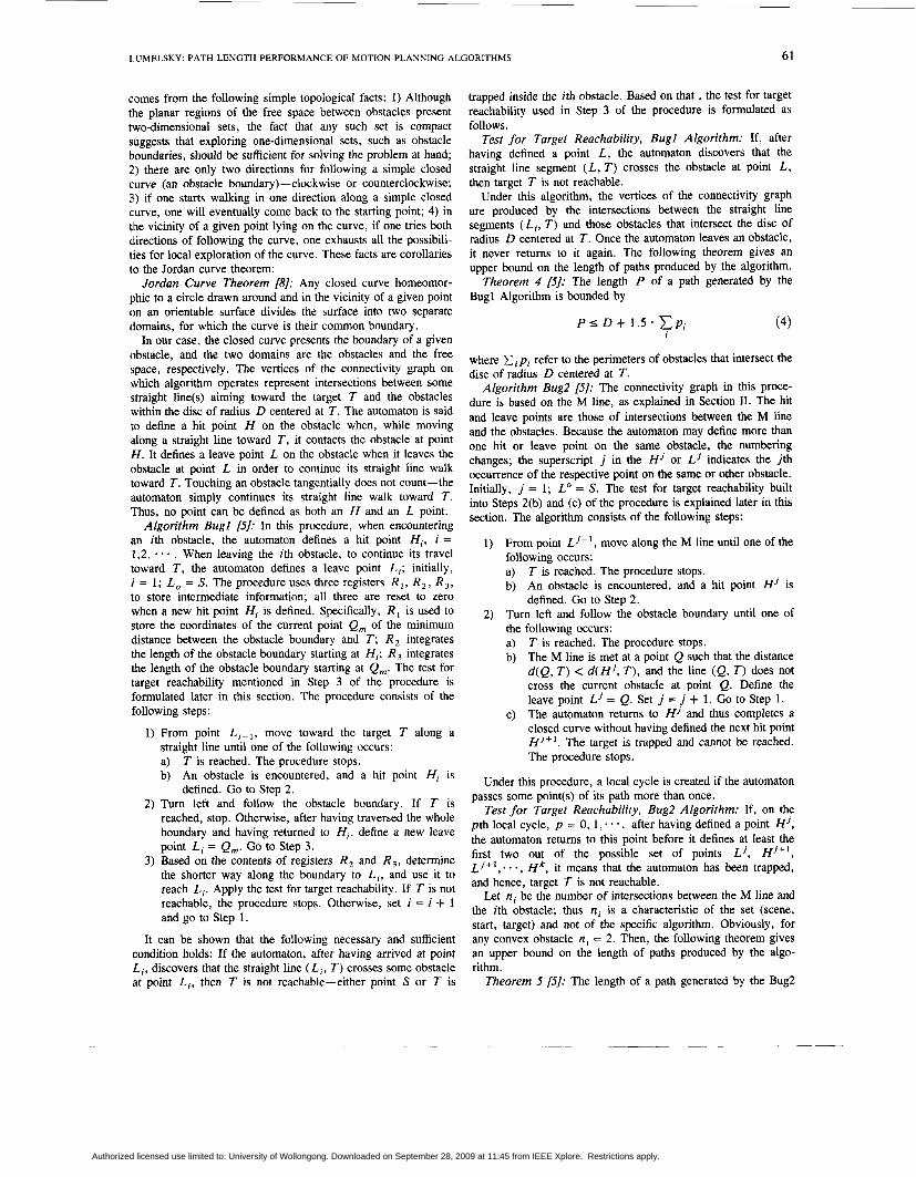
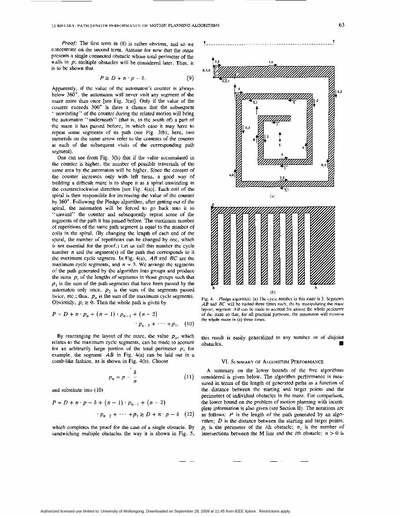
One can see from Fig. 3(b) that if the value accumulated in the counter is higher, the number of possible traversals of the same area by the automaton will be higher. Since the content of the counter increases only with left turns, a good way of building a difficult maze is to shape it as a spiral unwinding in the counterclockwise direction [see Fig. 4(a)]. Each coil of the spiral is then responsible for increasing the value of the counter by 360”. Following the Pledge algorithm, after getting out of the spiral, the automaton will be forced to go back into it to “unwind” the counter and subsequently repeat some of the segments of the path it has passed before. The maximum number of repetitions of the same path segment is equal to the number of coils in the spiral. (By changing the length of each end of the spiral, the number of repetitions can be changed by one, which is not essential for the proof.) Let us call this number the cycle number n and the segment(s) of the path that corresponds to it the maximum cycle segment. In Fig. 4(a), AB and BC are the maximum cycle segments, and n = 3. We arrange the segments of the path generated by the algorithm into groups and produce the sums pi of the lengths of segments in those groups such that p, is the sum of the path segments that have been passed by the automaton only once, p2 is the sum of the segments passed twice, etc.; thus, pn is the sum of the maximum cycle segments. Obviously, pi 2 0. Then the whole path is given by

By rearranging the layout of the maze, the value pn, which relates to the maximum cycle segments, can be made to account for an arbitrarily large portion of the total perimeter p; for example, the segment AB in Fig. 4(a) can be laid out in a comb-like fashion, as is shown in Fig. 4(b). Choose

6 p = p - -

n and substitute into (10)

P = D + n * p - 6 + ( n - 1) * p n - ] + ( n - 2 )

.p,-, + * * a +p1 2 D + TI ‘ p - 6 (12)

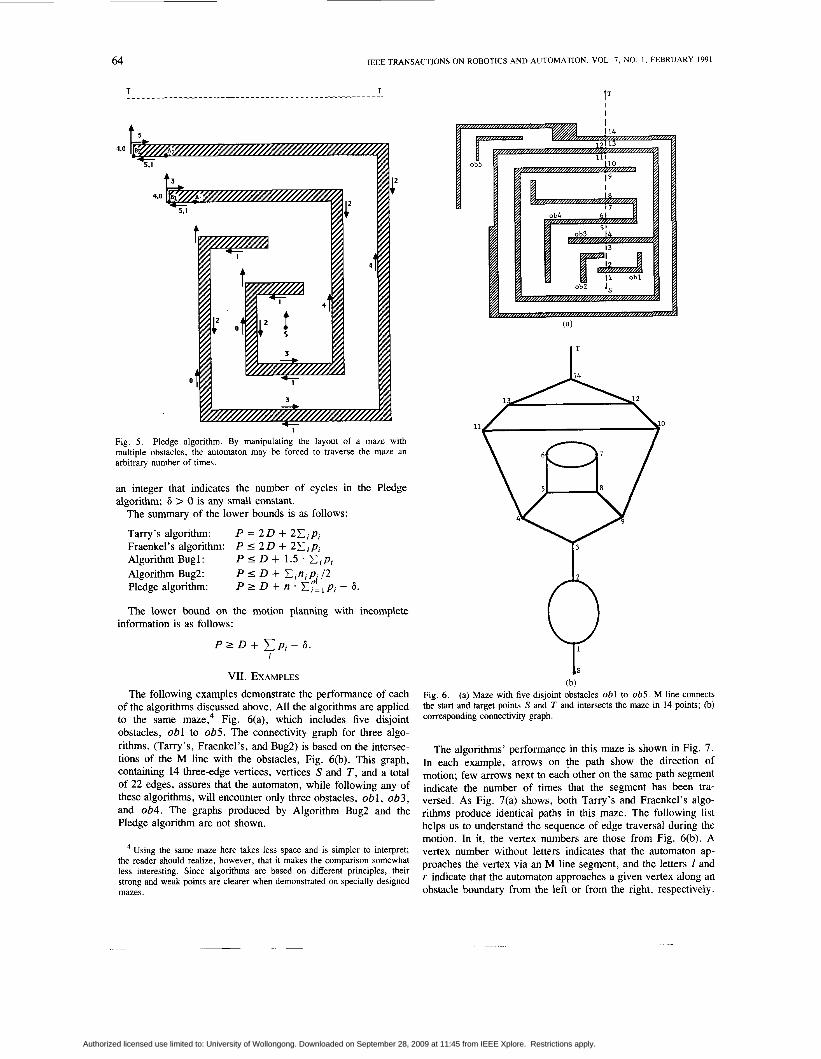
which completes the proof for the case of a single obstacle. By sandwiching multiple obstacles the way it is shown in Fig. 5,

8.4.0

~

63

C

B A

(b) Fig. 4. Pledge algorithm: (a) The cycle number in this maze is 3. Segments AB and BC will be visited three times each; @) by manipulating the maze layout, segment AB can be made to account for almost the whole perimeter of the maze so that, for all practical purposes, the automaton will traverse the whole maze in (a) three times.

this result is easily generalized to any number m of disjoint obstacles. rn

VI. SUMMARY OF ALGORITHM PERFORMANCE A summary on the lower bounds of the five algorithms

considered is given below. The algorithm performance is mea- sured in terms of the length of generated paths as a function of the distance between the starting and target points and the perimeters of individual obstacles in the maze. For comparison, the lower bound on the problem of motion planning with incomplete information is also given (see Section 11). The notations are as follows: P is the length of the path generated by an algorithm; D is the distance between the starting and target points; pi is the perimeter of the ith obstacle; ni is the number of intersections between the M line and the ith obstacle; n > 0 is



T I = 1

I I

Fig. 5 . Pledge algorithm. By manipulating the layout of a maze with multiple obstacles, the automaton may be forced to traverse the maze an arbitrary number of times.

an integer that indicates the number of cycles in the Pledge algorithm; 6 > 0 is any small constant.

The summary of the lower bounds is as follows:

Tarry’s algorithm: Fraenkel’s algorithm: Algorithm Bugl: Algorithm Bug2: Pledge algorithm:

The lower bound on the motion planning with incomplete

P = 2 0 + 2 C i p i P 5 2 D + 2 1 pi P 5 D + 1.5 * C i p i P 5 D + Cini Pi 12 P 2 D + n * Cy= pi - 6.

information is as follows:

P r D + C p i - 6 . i

VI1 . EXAMPLES The following examples demonstrate the performance of each

of the algorithms discussed above. All the algorithms are applied to the same maze,4 Fig. 6(a), which includes five disjoint obstacles, ob1 to ob5. The connectivity graph for three algorithms, (Tarry’s, Fraenkel’s, and Bug2) is based on the intersections of the M line with the obstacles, Fig. 6(b). This graph, containing 14 three-edge vertices, vertices S and T , and a total of 22 edges, assures that the automaton, while following any of these algorithms, will encounter only three obstacles, obl , ob3, and ob4. The graphs produced by Algorithm Bug2 and the Pledge algorithm are not shown.

Using the same maze here takes less space and is simpler to interpret; the reader should realize, however, that it makes the comparison somewhat less interesting. Since algorithms are based on different principles, their strong and weak points are clearer when demonstrated on specially designed mazes.

I’

(b) Fig. 6. (a) Maze with five disjoint obstacles ob1 to ob5. M line connects the start and target points S and T and intersects the maze in 14 points; (b) corresponding connectivity graph.

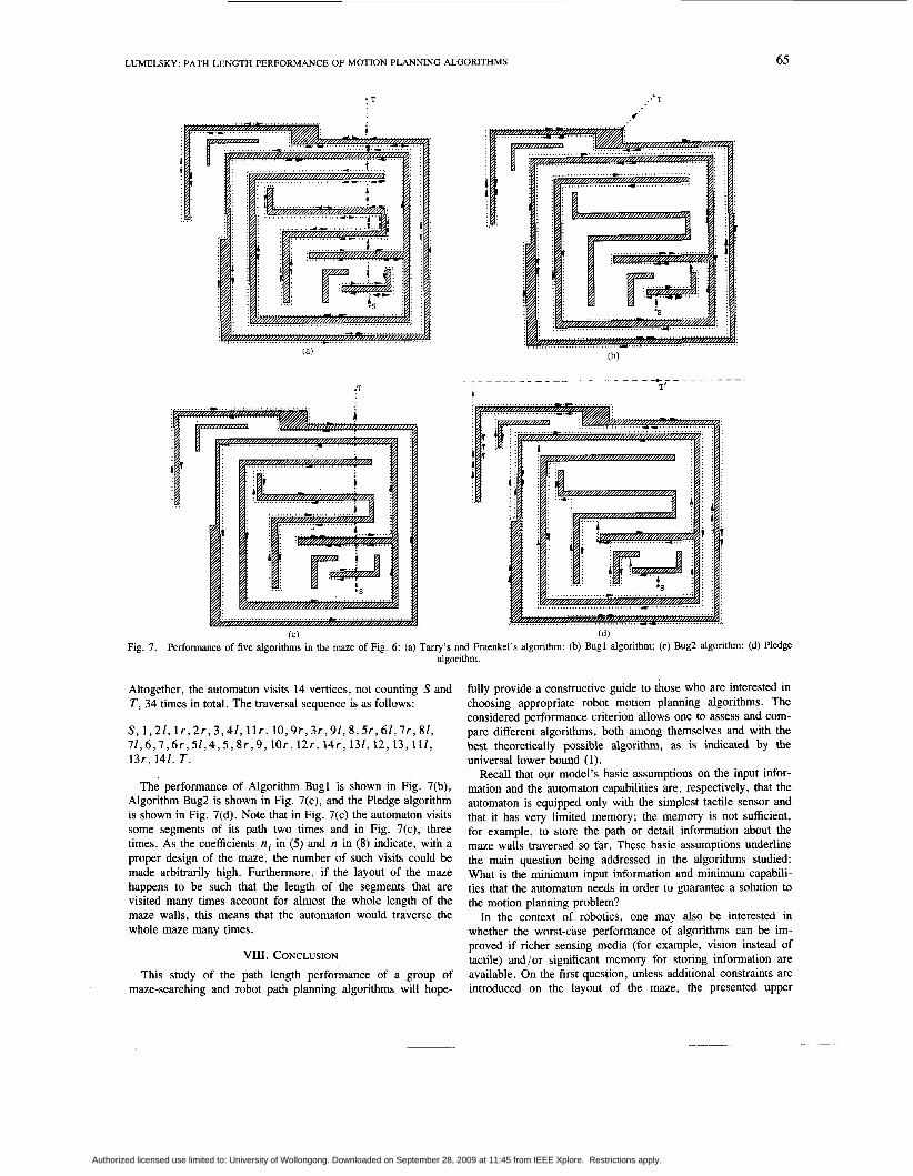
The algorithms’ performance in this maze is shown in Fig. 7. In each example, arrows on the path show the direction of motion; few arrows next to each other on the same path segment indicate the number of times that the segment has been traversed. As Fig. 7(a) shows, both Tarry’s and Fraenkel’s algorithms produce identical paths in this maze. The following list helps us to understand the sequence of edge traversal during the motion. In it, the vertex numbers are those from Fig. 6(b). A vertex number without letters indicates that the automaton approaches the vertex via an M line segment, and the letters I and r indicate that the automaton approaches a given vertex along an obstacle boundary from the left or from the right, respectively.



‘ T

Fig. 7. Performance of five algorithms in the maze of Fig. 6: (a) Tarry’s and Fraenkel’s algorithm: (b) Bugl algorithm; (c) Bug2 algorithm; (d) Pledge algorithm.

Altogether, the automaton visits 14 vertices, not counting S and T , 34 times in total. The traversal sequence is as follows:

S , 1 , 2 l , l r , 2 r , 3,41, l l r , 10 ,9 r , 3 r , 9 1 , 8 , 5 r , 61,7r , 81, 71 ,6 ,7 ,6 r , 5 1 , 4 , 5 , 8 r , 9 , lor, 12r , 14 r , 131,12,13,111, 13r, 141, T .

The performance of Algorithm Bugl is shown in Fig. 7(b), Algorithm Bug2 is shown in Fig. 7(c), and the Pledge algorithm is shown in Fig. 7(d). Note that in Fig. 7(c) the automaton visits some segments of its path two times and in Fig. 7(c), three times. As the coefficients ni in (5) and n in (8) indicate, with a proper design of the maze, the number of such visits could be made arbitrarily high. Furthermore, if the layout of the maze happens to be such that the length of the segments that are visited many times account for almost the whole length of the maze walls, this means that the automaton would traverse the whole maze many times.

VIII. CONCLUSION This study of the path length performance of a group of

maze-searching and robot path planning algorithms will hope-

fully provide a constructive guide to those who are interested in choosing appropriate robot motion planning algorithms. The considered performance criterion allows one to assess and compare different algorithms, both among themselves and with the best theoretically possible algorithm, as is indicated by the universal lower bound (1).

Recall that our model’s basic assumptions on the input information and the automaton capabilities are, respectively, that the automaton is equipped only with the simplest tactile sensor and that it has very limited memory; the memory is not sufficient, for example, to store the path or detail information about the maze walls traversed so far. These basic assumptions underline the main question being addressed in the algorithms studied: What is the minimum input information and minimum capabilities that the automaton needs in order to guarantee a solution to the motion planning problem?

In the context of robotics, one may also be interested in whether the worst-case performance of algorithms can be improved if richer sensing media (for example, vision instead of tactile) and/or significant memory for storing information are available. On the first question, unless additional constraints are introduced on the layout of the maze, the presented upper


66 IEEE TRANSACTIONS ON ROBOTICS AND AUTOMATION, VOL. 7 , NO. 1 , FEBRUARY 1991

bounds for the algorithms are not affected by improved sensing. This is simply because a “tough” maze can always be designed that would defeat any richer sensing media. On the second question, again, if no additional constraints are imposed on the shape of the maze walls, in principle, storing such information would require an infinite memory. On the other hand, if the maze walls can be assumed to be “not too wavy” and suffi- ciently distant, on the average, from each other, one can take advantage of the additional capabilities -for example, to elimi- nate local cycles in Algorithm Bug2 and the Pledge algorithm (see also [13] on incorporating proximity and vision sensing in the motion planning function).

From the presented analysis, one can draw the following conclusions:

Different algorithms produce very different paths, and in general, no one is a substitute for the other. In terms of the worst-case performance, Algorithm Bug1 is the best that can be offered today. Its better performance comes from exploiting specifics of maze topology -that the corresponding connectivity graph is of special structure, with each vertex having exactly three edges incident to it. However, in an “average” maze, other algorithms may exhibit better performance. In princible, algorithms that have unbounded worst-case performance, such as Bug2 and the Pledge algorithm, are more risky-in an unfortunate case, they can produce very long paths. Thus, one possible strategy is that unless some additional information about the topology of the maze suggests that the risk is warranted, they should be avoided. On the other hand, a more adventurous strategist may argue that these algorithms are better because in more typical mazes, their performance can significantly exceed that of other algorithms; after all, mazes that are “dangerous” for the Bug2 and Pledge algorithms are rather special and rare. Still ahother approach is to try to combine better features of different algorithms in a single procedure (see [5 ] for one such procedure).

ACKNOWLEDGMENT The author wishes to thank A. Stepanov for good discussions

and T. Skewis for bringing Tarry’s algorithm to the author’s attention and for generating clever counter examples.

REFERENCES [ l ] C. Yap, “Algorithmic motion planning,” in Advances in

Robotics, I: Algorithmic and Geometric Issues, J . Schwartz and C. Yap, Eds. Hillsdale, NJ: L. Erlbaum Associates, 1987. L. Budah, “Environments, labyrinths, and automata,” in Fun- [2]

damentals of Computation Theory, Karpinsky, Ed. New York: Springer Verlag, 1977, pp. 54-64. M. Blum and D. Kozen, “On the power of the compass (or, why mazes are easier to search than graphs),” in Proc. 19th Ann. Symp. Foundations of Comput. Sci. (FOCS) (Ann Arbor, MI), 1978. H. Abelson and A. diSessa, Turtle Geometry. Cambridge, MA: MIT Press, 1980, pp. 176-199. V. Lumelsky and A. Stepanov, “Path planning strategies for a point mobile automaton moving amidst unknown obstacles of arbitrary shape,” Algorithrnica, vol. 2, pp. 403-430, 1987. V. Lumelsky, “Effect of kinematics on dynamic path planning for planar robot arms moving amidst unknown obstacles,” IEEE J . Robotics Automat., vol. RA-3, pp. 207-223, 1987. A. S . Fraenkel, “Economic traversal of labyrinths,” Math. Mag., vol. 43, pp. 125-130, 1970; vol. 44, p. 12, 1971. H. Behnke et al., Eds., Fundamentals of Mathematics. Cam- bridge, MA: MIT Press, 1974, vol. 11, Geometry, ch. 16, Topology. A. Aho, J. Hopcroft, and J. Ullman, The Design and Analysis of Computer Algorithms. Reading, MA: Addison-Wesley,

R. Aleliunac, R. Karp, R. Lipton, L. Lovasz, and C. Rackoff, “Random walks, universal traversal sequences, and the complexity of maze problems,” in Proc. 20 Symp. Foundations Com- put. Science (FOCS), 1979. 0. Ore, Theory of Graphs. Providence, RI: Amer. Math. Society, 1962. C. Berge, Graphs and Hypergraphs. Amsterdam: North-Hol- land, 1973. V. Lumelsky and T. Skewis, “Incorporating range sensing in the robot navigation function,” IEEE Trans. Syst., Man, Cybern., vol. 20, no. 5, pp. 1058-1069, Sept./Oct. 1990.

1974, pp. 172-198.

Vladimir J. Lumelsky (M’80-SM’83) received the B.S. and M.S. degrees in electrical engineering and computer science in Leningrad in 1962, and the Ph.D. degree in applied mathematics from the Institute of Control Sciences (ICs), U.S.S.R. National Academy of Sciences, Moscow, in 1970.

From 1967 to 1975, he held academic positions in ICs conducting research in pattern recognition, factor analysis, and control systems. From 1976 to 1980, he was on the re-

search staff at Ford Motor Company Scientific Laboratories, Dearborn, MI. From 1980 to 1985, he was with the General Electric Research Center, Schenectady , NY, doing research in robotics, image processing, pattern recognition, control theory, and industrial automation. Since 1985, he has been on the faculty of the Department of Electrical Engineering at Yale University. His research interests are in robotics, image processing, pattern recognition, and control theory.

Dr. Lumelsky is a member of the Editorial Board of the IEEE TRANSACTIONS ON ROBOTICS AND AUTOMATION and of the Board of Governors of the IEEE Society of Robotics and Automation. He is a member of the ACM and Robotics International of SME.


Documents

A comparative study on the path length performance of maze ......A~stract-Maze-searching algorithms first appeared in graph theory and, more recently, have been studied in works on