International Journal on Electrical Engineering and Informatics - Volume 8, Number 4, December 2016

A Comparative Study on Decomposition of Test Signals Using Variational

Mode Decomposition and Wavelets

Anusha S1, Ajay Sriram

1, and T Palanisamy

2

1Department of Electrical and Electronics Engineering,

2Department of Mathematics, Amrita School of Engineering- Coimbatore,

Amrita Vishwa Vidyapeetham, Amrita University, India

Abstract: The decomposition of signals into their primitive or fundamental constituents play a

vital role in removing noise or unwanted signals, thereby improving the quality and utility of

the signals. There are various decomposition techniques, among which the linear wavelet

technique and the Variational Mode Decomposition (VMD) are the most recent and widely

used ones. This paper presents a comparative study of the decomposition of spatially

inhomogeneous test functions namely Doppler and Bumps used by statisticians. An effort is

made in this article to compare the efficiency of the noise removal in the resulting

decompositions at various approximation levels using wavelets and by varying the number of

reconstruction modes in VMD. Surprisingly it is found that the VMD technique yields better

results with more accuracy for a specific set of parameters irrespective of the spatial character

of the function.

Keywords: Variational mode decomposition, Doppler, Bumps.

1. Introduction

Myriads of techniques exist, for a signal to be processed and analyzed. Decomposition is

one such technique, which includes determining the number of signals present, their epochs

and amplitudes. The key idea of analysis is to represent signals as a superposition of simpler

signals so that each such signal can be operated upon independently. The motivation for our

work arose from the investigations of brain waves such as electroencephalogram and visual

evoked responses, the desire to distinguish between multiple echoes in a noisy environment in

radar and sonar and the need to locate the seismic source in seismology where the data consists

of the arrivals of various waves. Under all such occasions, there has been a requirement to seek

methods by which composite waveforms may be decomposed[1]. However, the digital data

decomposition involves plethora of problems like filter realizability, signal resolution

capability, the effects of additive noise and a frequency (spectrum) compatibility between

signal waveform and filter response pulse. Such problems can be dealt by implementing

various linear filter operations and decomposition techniques.

For signals that are to be processed, the prior knowledge about the characteristics of the

signal is either known or unknown. Even when the knowledge about the signal is known,

information about its spatial homogeneity may still be unknown. Spatially inhomogeneous

functions may have, for example, jump discontinuities and high frequency oscillations [2].

Such functions might require a greater amount of smoothing in some portions of the domain,

and less smoothing in other places [3].However, various techniques exist for signal processing

to be carried out with or without prior details. Our effort in this paper is to identify a

decomposition technique that would yield efficient denoising results inspite of the absence of

prior knowledge or spatial homogeneity. For this purpose, we make a comparison between the

widely used linear wavelet techniques and the recently developed Variational Mode

Decomposition(VMD) [4] by employing them on the standard test functions, Bumps and

Doppler defined by Donoho & Johnstone (1994) . These functions have been particularly

chosen because they caricature spatially variable functions arising in imaging, spectroscopy

and other scientific signal processing [5]. Similar signal decomposition techniques that are

Received: September 4th

, 2016. Accepted: December 23rd

, 2016

DOI: 10.15676/ijeei.2016.8.4.13

885

based on linear wavelets have been used for ECG signals [6], for smoothing noisy data [7-8]

and for curve estimation [9]. We present this study on decomposition of spatially

inhomogeneous signals using VMD and linear wavelet techniques to compare the efficiency of

noise removal that has not been attempted so far.

The rest of the paper is organized as follows. Section 2 briefly reviews about wavelets and

VMD. The comparison between decomposition techniques discussed above is explained in

Section 3. The observations made in our study is summarized and concluded in Section 4.

2. Review of Wavelet and VMD

A. Wavelet

In this sub-section we give a brief review of wavelet theory, on which the function

representation is to be made. Wavelet decomposition method is motivated by the fact that the

important information appears through a simultaneous analysis of the signal 's time and

frequency properties[10]. In fact, the ability of Fourier analysis to go from time domain to

frequency domain and to have a dictionary that allows us to infer properties in one domain

from the information in the other domain revolutionized mathematics. But, when computing

the Fourier coefficients all values of the function in time domain are taken into account for

each frequency and therefore frequency information is obtained at the cost of time information.

This drawback of Fourier transform can be overcome by constructing a complete orthonormal

set in ),(2 RL the collection of all square integrable functions defined over 𝑅of the form

Zkjkj ,, }{ for some ),(2 RL known as wavelet system. They are compactly supported and

band limited. For this purpose Mallat[11] determined the conditions that a sequence of

embedded vector spaces }:{ ZjV j should satisfy. Under these conditions the sequence will

become a multi-resolution analysis (MRA) which in turn yields a compactly supported wavelet

system. Since, MRA requires 10 VV and if }:)2(2{ ,1 Zkktk is a complete

orthonormal set in ,1V for some ,0V such that

R

dtt ,1)( we can express

k

Zk

ku ,1)(

. Letting

Zk

kkvt ,1)()( where )1()1()(:)({ kukvkvv k and

Zk

k ZlzkzW )(:)( 2

,00 where )(2 Zl is the collection square summable

sequences, we can easily see that }:)({ Zkkt is orthonormal to }:)({ Zkkt .

This W0 is the complement of V0inV1 and is obviously orthonormal to 0V and hence

.001 WVV If jW is the subspace spanned by }:)2(2{ 2 Zkktj

j

then it can be shown

that Wj is orthogonal complement of jV in 1jV for every Zj . Obviously, Wj’s are not

nested but ...... 10 WW As a result jZjWRL

)(2 and j

mj

mn WVV

1

for nm .

Therefore, },:)2(2{ 2 Zkjktj

j

forms an orthonormal basis for ).(2 RL Thus the MRA

eventually yields an orthonormal basis which consists of functions known as wavelets. The

projection of any function of )(2 RL in jV can be thought of as the approximation of that

Anusha S, et al.

886

function and the projection over jW gives the detail to go over to the next approximation level

in .1jV This enables us to view any function of )(2 RL in various resolutions.

B. Variational Mode Decomposition

In this section, we give a brief review of VMD. This technique decomposes the given

function f into various components 𝑓𝑘 for 𝑘 = 1,2, … 𝐾 known as modes using calculus of

variation. The Fourier transform of each component of the function 𝑓𝑘is assumed to have

compact support around the mean of the independent variable of the Fourier transform. This is

otherwise known as the central frequency[12] and is denoted by𝜔𝑘 .VMD will find out these

central frequencies and the components centered on those frequencies concurrently by

minimizing the sum of the lengths of the supports ∆𝜔𝑘 of the Fourier transforms or bandwidths

of components subject to the condition that sum of the components is equal to the given

function. For this purpose, we construct an analytic function corresponding to the original

component 𝑓𝑘(𝑡)as𝑓𝑘(𝑡) + j𝑓𝑘𝐻(𝑡) by finding the Hilbert Transform 𝑓𝑘

𝐻 of the component 𝑓𝑘

which in fact forms the conjugate harmonic of the component 𝑓𝑘 . For the sake of convenience,

we wish to shift the bandwidth of the analytic signal 𝑓𝑘𝐴(𝑡) for k = 1,2,...K, from ωk to 0. This

can be accomplished by multiplying the analytic function 𝑓𝑘𝐴 with the complex exponential

𝑒−𝑗𝜔𝑘𝑡.Further, we know that the measure of bandwidth of the components can be calculated

by finding the integral of the square of the time derivative of the frequency-translated function

component

𝑓𝑘𝐷(𝑡) = 𝑓𝑘

𝐴(𝑡)𝑒−𝑗𝜔𝑘𝑡

𝑖. 𝑒. ∆𝜔𝑘 = ∫(𝜕𝑡( 𝑓𝑘𝐷))(𝜕𝑡(𝑓𝑘

𝐷))̅̅ ̅̅ ̅̅ ̅̅ ̅̅ 𝑑𝑡

= ∫ |𝜕𝑡(𝑓𝑘𝐷)|2𝑑𝑡

= ||𝜕𝑡(𝑓𝑘𝐷)||

2

2

Thus, the bandwidth is the squared L2 norm of the gradient of the demodulated function

components [13].Therefore, the required minimization problem is

𝑚𝑖𝑛

𝑓𝑘,𝜔𝑘,∑||𝜕𝑡(𝑓𝑘

𝐷)||2

2 𝑠𝑢𝑐ℎ 𝑡ℎ𝑎𝑡

𝑘

∑ 𝑓𝑘

𝑘

= 𝑓

𝑖. 𝑒.𝑚𝑖𝑛

𝑓𝑘,𝜔𝑘,∑ ||𝜕𝑡[((𝛿(𝑡) + 𝑗/𝜋𝑡) ∗ 𝑓𝑘(𝑡))𝑒−𝑗𝜔𝑘𝑡]||

2

2

𝑘

𝑠𝑢𝑐ℎ 𝑡ℎ𝑎𝑡 ∑ 𝑓𝑘

𝑘

= 𝑓

The above constrained optimization problem will be solved by converting into

unconstrained optimization problem. In fact, we find the central frequencies 𝜔𝑘 for 𝑘 =1,2, … 𝐾and the respective modes by minimizing the sum of the bandwidths using augmented

Lagrangian method [14].

𝐿(𝑓𝑘, 𝜔𝑘 , 𝜆) = 𝛼𝑚𝑖𝑛

𝑓𝑘,𝜔𝑘∑||𝜕𝑡(𝑓𝑘

𝐷)||2

2

𝑘

+ ||𝑓 − ∑ 𝑓𝑘

𝑘

||22 + 𝜆(𝑓 − ∑ 𝑓𝑘

𝑘

)

where 𝛼 is the balancing parameter of the data-fidelity constraint and 𝜆 is the Lagrangian

multiplier. In fact, we can customize our optimization procedure of VMD based on our need.

In the next section, the decomposition of certain test functions are made using VMD and

wavelet decomposition techniques. The results are then analyzed by considering various modes

under varying bandwidth constraints and noise tolerance of VMD and various levels of

A Comparative Study on Decomposition of Test Signals Using Variational

887

different wavelets. Also a comparative study is carried out between the performance of VMD

and Wavelet.

3. Experimental Results

Two of the few test functions mainly used by statisticians, namely Doppler, with high

frequency oscillations and Bumps, with jump discontinuities, and the sine, a smooth function

are considered here for the analysis and comparison of performance between VMD and

wavelet decomposition. In fact we study the efficiency of VMD and wavelet decomposition

techniques in eliminating noise from the signal and a comparative study is also made. For this

purpose we add Gaussian noise to the Doppler and Bumps function respectively. While we

work with VMD technique, we have mainly considered three parameters, i.e., number of

modes, noise tolerance and bandwidth constraints, which are varied and applied on each

function, whose results are obtained using MATLAB. We have obtained results for the number

of reconstruction modes 2,3 and 4, for noise tolerance 0,1,2,3 and 4 and for bandwidth

constraints 100,90,75,50 and 30 for Doppler whereas for 2000,1000,500,100,90,50 and 30 for

Bumps. In wavelet decomposition technique we have used three wavelets, namely coiflet of

order 5,4 and 3, for each of which we have varied the approximation levels through 2,3,4,5,6

and 7. The efficiency of noise removal of the above discussed techniques over these test

functions made us review the performance of these decomposition techniques over a smooth

function as well.

A. Results based on Variational Mode Decomposition

A.1. Results of Doppler

When we used VMD over Doppler, we varied initially the bandwidth constraint(𝛼)for

modes 2,3 and 4 and for fixed noise tolerance(𝜏). We used the mean square error (MSE) to

study the performance. The conclusion so obtained on the bandwidth constraint show that the

resulting MSE is better for 𝛼 < 100. Hence we found out the result by varying bandwidth

constraint 𝛼 = 90, 𝛼 = 75, 𝛼 = 50 𝑎𝑛𝑑 𝛼 = 30. The best result was found to be for the mode,

𝑘 = 2 at 𝛼 = 30 for fixed noise tolerance 𝜏 = 0, which is shown in Table 1. Further, we kept

the bandwidth constraint constant at 𝛼 = 30and the noise tolerance was increased which is

shown in Table 2. The MSE was found to be negligible for the noise tolerance 𝜏 = 4and 𝑘 = 2.

The plot of original Doppler function embedded on the first mode of VMD are depicted in

Figure 1 for the parameters = 2 , 𝛼 = 30 and 𝜏 = 0 and in Figure 2 for parameters 𝑘 = 2,

𝛼 = 30 and 𝜏 = 4.

Table 1. Variation in Bandwidth Constraint

No. of modes α = 100 α = 90 α = 75 α = 50 α = 30

K=2 0.0852 0.0862 0.072 0.069 0.046

K=3 0.1742 0.1654 0.151 0.0969 0.062

K=4 0.207 0.19623 0.1928 0.1642 0.1466

Table 2. Variation in noise tolerance

No. of modes (k) τ =1 τ =2 τ =3 τ =4

K=2 0.011 0.012 0.0101 0.010

K=3 0.063 0.065 0.064 0.067

K=4 0.1359 0.1372 0.1352 0.1321

Anusha S, et al.

888

Figure 1

Figure 2

A.1.2 Results of Bumps test function

For Bumps, when the bandwidth constraint 𝛼 is varied on a scale from 2000 to 30, choosing

certain intermediate values, it is seen that the MSE goes on decreasing with decreasing α value,

which is shown in Table 3. Thus, the bandwidth constraint is fixed at a value of 30 and the

performance is analyzed for different noise tolerance 𝜏 = 1, 𝜏 = 2, 𝜏 = 3 and 𝜏 = 4, with

number of modes taken as 2,3 and 4 under each case which is shown in Table 4. It is seen that

the least MSE occurs for 𝜏 = 2, 𝑘 = 2. The plot of original Bumps function embedded on the

A Comparative Study on Decomposition of Test Signals Using Variational

889

first mode of VMD are depicted in Figure 3 for the parameters = 2 , 𝛼 = 30 and 𝜏 = 0 and in

Figure 4 for parameters 𝑘 = 2 , 𝛼 = 30 and 𝜏 = 4.

Table 3. Variation in Bandwidth constraint

No. of

modes (k)

𝜶 = 𝟐𝟎𝟎𝟎

𝜶 = 𝟏𝟎𝟎𝟎

𝜶 = 𝟓𝟎𝟎

𝜶 = 𝟏𝟎𝟎

𝜶 = 𝟗𝟎

𝜶 = 𝟓𝟎

𝜶 = 𝟑𝟎

𝑲 = 𝟐 0.1795 0.1648 0.1577 0.1159 0.1045 0.0811 0.0668

𝑲 = 𝟑 0.1858 0.1779 0.1739 0.1529 0.1563 0.1392 0.1356

𝑲 = 𝟒 0.1886 0.1854 0.1813 0.1689 0.1669 0.1656 0.1596

Figure 3.

Figure 4

Anusha S, et al.

890

Table 4. Variation in noise tolerance No. of

modes (k) 𝝉 = 𝟏 𝝉 = 𝟐 𝝉 = 𝟑 𝝉 = 𝟒

𝑲 = 𝟐 0.0244 0.0237 0.024108 0.025745

𝑲 = 𝟑 0.103487 0.0936 0.0842 0.086071

𝑲 = 𝟒 0.1492 0.1486 0.150116 0.150646

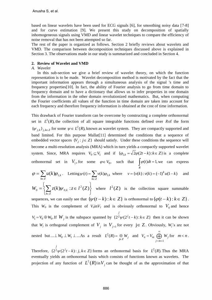
B. Results based on Wavelets

When wavelet techniques are used over the considered test functions, the decompositions at

various approximation levels are obtained using coiflet of order 3,4 and 5 and analyzed. For

both Doppler and Bumps, we see that the MSE is the least for second level, under coiflet of all

orders analyzed, i.e., lower the approximation level, lower the MSE. It is also observed that

among coiflet of order 3,4 and 5, coiflet of order 5 yields better results than the other ones. The

plot of original Doppler function embedded on the seventh and second approximation level of

coiflet wavelet of order 5 are depicted in Figure 5 and in Figure 6, for the plot of original

Bumps function embedded on the seventh and second approximation level of coiflet wavelet of

order 5.

B.1 Wavelet results of Doppler

Figure 5(a)

A Comparative Study on Decomposition of Test Signals Using Variational

891

Figure 5(b)

B.2 Wavelet results of Bumps

Table 6. Variation in levels of various wavelets for bumps function

Wavelets Level 7 Level 6 Level 5 Level 4 Level 3 Level2

Coif5 0.2313 0.1617 0.0629 0.0213 0.0063 0.0034

COif4 0.2308 0.1618 0.0671 0.0251 0.0053 0.0032

Coif3 0.2293 0.1620 0.0694 0.0228 0.0067 0.0034

Figure. 6(a)

Anusha S, et al.

892

Figure. 6(b)

C. Wavelet and VMD for a smooth curve

Because of the difference in the nature of smoothness of the test functions namely Doppler

and Bumps, we got motivated to study the performance of the above discussed decomposition

techniques also over a smooth function. Hence, we considered 𝑓(𝑥) = 𝑠𝑖𝑛𝑥 for the analysis of

Wavelet and VMD techniques in order to conclude their performances over smooth and non-

smooth functions.

Table 7. Variation in Bandwidth constraint and noise tolerance of sine function No. of

modes(𝐾) 𝛼 = 2000

𝜏 = 0

𝛼 = 1000 𝜏 = 0

𝛼 = 500 𝜏 = 0

𝛼 = 100 𝜏 = 0

𝛼 = 90 𝜏 = 0

𝛼 = 50 𝜏 = 0

𝛼 = 30

𝜏 = 4 𝐾 = 2 0.001847 0.000639 0.000231 0.000022 0.000013 0.000004 0.000001

𝐾 = 3 0.002137 0.000736 0.000265 0.000025 0.000020 0.000001 0.000000

𝐾 = 4 0.002522 0.000895 0.000322 0.000031 0.000026 0.000001 0.000000

Table 8. Variation in levels of various wavelets for sin function

Wavelets Level

2

Level

4

Level

5

Level

6

Level

8

Level

10

Coif5 0.5516 0.5304 0.4875 0.3887 0.2615 0.098

COif4 0.5516 0.5264 0.4834 0.388 0.2585 0.143

Coif3 0.5532 0.5289 0.4814 0.3882 0.2548 0.1454

When the VMD technique is applied over sine function, the MSE decreases as the

bandwidth constraint decreases and an increase in noise tolerance results in an decreasing

MSE. The least error is obtained at the same case as obtained for the specific test functions

Doppler and Bumps. Further, in the case of wavelet technique the MSE decreases when the

approximation level increases for the sine function and it is found that MSE obtained by

varying the approximation levels of various wavelets is comparatively more than the MSE

obtained by VMD. Also it is interesting to note that the MSE is less for higher approximation

levels in case of smooth function whereas the MSE is found to be less for lower approximation

levels in case of specific test functions.

A Comparative Study on Decomposition of Test Signals Using Variational

893

4. Conclusion

We performed the VMD and Wavelet based noise removal over spatially inhomogeneous

test functions, Doppler with high frequency oscillations and Bumps with jump discontinuities.

Also, we have performed the wavelet and VMD based noise removal on sine function to

observe their performances on a spatially homogeneous function and thereby we extended our

study to spatially homogeneous functions as well in order to compare the performance of these

techniques with spatially homogeneous or inhomogeneous functions. Our study reveals that the

VMD technique yields better results when the parameters namely the number of modes 𝑘 = 2,

bandwidth constraint 𝛼 = 30and noise tolerance 𝜏 = 4, despite the spatial characteristics of the

function. Thus the VMD technique performs equally well for all the functions that we studied,

irrespective of the spatial inhomogeneity and thus with or without prior knowledge for the

afore mentioned parameters. On the other hand, while we used linear wavelet techniques, the

best results for Doppler and Bumps were obtained at level 2 whereas for the sine function, it

was obtained at level 10. Thus, the approximation levels of linear wavelet techniques are varied

to get better results depending upon the spatial characteristics of the function.

From the above discussion, we note that the VMD technique performs on par with linear

wavelet techniques for the spatially homogeneous functions and VMD performs better than the

linear wavelet technique in the case of spatially inhomogeneous functions. Also, as better

results are obtained in VMD technique for the same parameters despite the spatial

characteristics of the signal, the prior knowledge of the signal is not required. Hence our

comparative study concludes based on the efficiency of noise removal on these functions that

in the case of signals without prior knowledge or when the signal is spatially inhomogeneous,

VMD technique will result in better recovery of the signal than the linear wavelet technique

after the noise removal.

5. References

[1]. Childers, D. G., Varga, R. S. and Perry.N. W. (1970). Composite Signal

Decomposition. IEEE Transactions on Audio and Electroacoustics. vol. AU-18, No. 4:

471-477.

[2]. Palanisamy. T., (2016). Smoothing the Difference-based Estimates of Variance

UsingVariational Mode Decomposition.Communications in Statistics - Simulation and

Computation ,(In Press)

[3]. R.Todd Ogden. (1997). Essential wavelets for Statistical Applications and Data Analysis.

Birkhäuser.

[4]. Dragomiretskiy, K. and Zosso, D. (2014). Variational Mode Decomposition. IEEE

Transactions on Signal Processing. 2:531-544.

[5]. Donoho, D. L. and Johnstone I. M \(1994). Ideal Spatial Adaptation by Wavelet

Shrinkage.Biometrika, Vol. 81, No. 3: 425-455.

[6]. Sadhukhan, D. and Mitra, M. (2014). ECG Noise Reduction Using Linear and Non-linear

Wavelet Filtering.Proc. of Int. Conf. on Computing, Communication & Manufacturing.

2014

[7]. Amato U and Vuza D.T. (1994). Wavelet Regularization for Smoothing Data. Technical

report N. 108/94, Instituto per ApplicazionidellaMatematica, Napoli.

[8]. Antoniadis, A. (1994). Smoothing noisy data with coiflets.StatisticaSinica4 (2),651-678.

[9]. Antoniadis, A. and Gregoire, G. and Mckeague, I. (1994). Wavelet methods for curve

estimation. J. Amer. Statist. Assoc. 89 (428), 1340-1353.

[10]. Palanisamy, T. and Ravichandran, J. (2015). A wavelet-based hybrid approach to estimate

variance function in heteroscedastic regression models. Stat. Papers. 56(3):911-932.

[11]. Mallat, S. G. (1989). Multiresolution approximations and wavelet orthonormal bases of

L2 (R). Transactions of the American Mathematical Society.Vol.315, No.1, 69-87

[12]. Aneesh C, S. K, Hisham P M, Soman, K. P. (2015). Performance comparison of

Variational Mode Decomposition over Empirical Wavelet Transform for the classification

Anusha S, et al.

894

of power quality disturbances using Support Vector Machine.Procedia Computer

Science.46:372-380.

[13]. Wang, Y. M. R, Xiang, J. and Zheng, W. (2015). Research on variational mode

decomposition and its application in detecting rub-impact fault of the rotor system.

Mechanical Systems and SignalProcessing.60-61:243-251.

[14]. Huang, N. E., Shen, Z., Long, S. R., Wu, M.. C., Shih, H. H., Zheng, Q., Yen,N. C.,

Tung, C. C. and.Liu. H. H. (1998). The empirical mode decomposition and the Hilbert

spectrum for nonlinear and non-stationary time series analysis.Proc. Royal Soc. A: Math.,

Phys. Eng. Sci.. vol. 454, no. 1971:. 903–995.

Anusha S was born in Trichy, Tamil Nadu, India. She is currently a senior

undergraduate student doing final project at the Department of Electrical

Engineering, Amrita Vishwa Vidyapeetham, Amrita University, Coimbatore,

India.

Ajay Sriram was born in Trichy, Tamil Nadu, India. He is currently doing

his Master’s in Electrical Engineering specializing in wireless systems at

KTH Royal Institute of technology under the Integrated Master’s programme

of Amrita Vishwa Vidyapeetham.

T. Palanisamy is currently working as Associate Professor in the

Department of Mathematics, Amrita School of Engineering - Coimbatore,

Amrita University, India. He obtained his Doctoral Degree from Amrita

University, Coimbatore. His area of research is estimation of variance

function in heteroscedastic regression models. His research interest also

includes regression analysis, signal processing and image processing using

wavelet techniques and sparse representation theory. Dr. Palanisamy has

published number of research articles in reputed National and International

Journals. He is also a reviewer for reputed journals in Statistics. He has organized an

International Conference on Applications of Fractals and Wavelets in January 2015.

A Comparative Study on Decomposition of Test Signals Using Variational

895