Embed Size (px)
Citation preview
A Comparative Study of VariousVersions of the SABR Model Adapted
to Negative Interest Rates
IRINA SHADRINA
Master’s Thesis to obtain the degree inActuarial Science and Mathematical FinanceUniversity of AmsterdamFaculty of Economics and BusinessAmsterdam School of Economics
Author: Irina ShadrinaStudent nr: 11088397Email: [email protected]
Date: July 23, 2017Supervisor: Prof. dr. L. J. van GastelSecond reader: Prof. dr. ir. M. H. Vellekoop

SABR Volatility Smile Interpolation — Irina Shadrina iii
Abstract
In this thesis we compare different extensions of the SABR modeladapted to negative interest rates. Namely, we introduce and discussanalytical properties of the Shifted SABR, the Normal SABR, the FreeBoundary SABR and the Mixture SABR models.To compare numerical outcomes of the models we compute approxima-tion formulae for the implied Normal volatility in terms of the modelsparameters and compare the quality of the volatility smile approxima-tion using data on swaptions as a benchmark.Computational results show that the approximation quality of the Dis-placed SABR model outperforms the other models. Moreover, in somespecial cases of the market data the approximation quality is onlysufficient for the Displaced SABR model. We also conclude that theHagan approach can not be used for calibration of the parameters ofthe Free Boundary SABR and Mixture SABR models.Finally, we conclude, using our quality estimation criteria, that theDisplaced SABR model is the most suitable model for modelling thevolatility smile in the presence of negative rates.
Keywords negative interest rates, Black’s model, Bachelier’s model, SABR model, Displaced
SABR model, Normal SABR model, Free Boundary SABR model, Mixture SABR model, swap-
tions
Contents
Preface vi
1 Introduction 1
1.1 Economic background . . . . . . . . . . . . . . . . . . . . . . . . . . . . 1
1.2 Problem statement . . . . . . . . . . . . . . . . . . . . . . . . . . . . . . 3
1.3 Thesis outline . . . . . . . . . . . . . . . . . . . . . . . . . . . . . . . . . 5
2 Interest rate derivatives 6
2.1 Market of interest rate derivatives . . . . . . . . . . . . . . . . . . . . . 6
2.2 Interest rates . . . . . . . . . . . . . . . . . . . . . . . . . . . . . . . . . 6
2.3 Interest rate derivatives . . . . . . . . . . . . . . . . . . . . . . . . . . . 7
3 Mathematical framework 9
3.1 Assumptions . . . . . . . . . . . . . . . . . . . . . . . . . . . . . . . . . 9
3.2 Ito calculus . . . . . . . . . . . . . . . . . . . . . . . . . . . . . . . . . . 9
3.3 Pricing under the risk neutral measure . . . . . . . . . . . . . . . . . . . 11
4 Implied volatility 13
4.1 Black’s model . . . . . . . . . . . . . . . . . . . . . . . . . . . . . . . . . 13
4.2 Bachelier’s model . . . . . . . . . . . . . . . . . . . . . . . . . . . . . . . 13
4.3 Implied volatility . . . . . . . . . . . . . . . . . . . . . . . . . . . . . . . 14
4.4 Comparison of Normal and Black volatilities . . . . . . . . . . . . . . . . 14
4.5 Volatility smile . . . . . . . . . . . . . . . . . . . . . . . . . . . . . . . . 15
4.6 Local volatility models . . . . . . . . . . . . . . . . . . . . . . . . . . . . 15
5 SABR model 17
5.1 Model definition . . . . . . . . . . . . . . . . . . . . . . . . . . . . . . . 17
5.2 Risk-neutral probability density function . . . . . . . . . . . . . . . . . . 18
5.3 Results of Hagan et. al. . . . . . . . . . . . . . . . . . . . . . . . . . . . 19
5.3.1 Impact of parameters . . . . . . . . . . . . . . . . . . . . . . . . 20
5.3.2 Problems with Hagan et. al. formula . . . . . . . . . . . . . . . . 20
5.4 Results of Antonov et. al. . . . . . . . . . . . . . . . . . . . . . . . . . . 20
5.5 Parameters calibration . . . . . . . . . . . . . . . . . . . . . . . . . . . . 21
5.5.1 Hagan’s formula . . . . . . . . . . . . . . . . . . . . . . . . . . . 21
5.5.2 Antonov’s formula . . . . . . . . . . . . . . . . . . . . . . . . . . 22
5.5.3 Fit to the market . . . . . . . . . . . . . . . . . . . . . . . . . . . 22
6 SABR extensions for negative interest rates 23
6.1 Displaced SABR . . . . . . . . . . . . . . . . . . . . . . . . . . . . . . . 23
6.1.1 Advantages of the Displaced SABR model . . . . . . . . . . . . . 24
6.1.2 Disadvantages of the Displaced SABR model . . . . . . . . . . . 24
6.2 Normal SABR . . . . . . . . . . . . . . . . . . . . . . . . . . . . . . . . 24
6.2.1 Hagan’s approximation formula . . . . . . . . . . . . . . . . . . . 24
6.2.2 Antonov’s explicit solution . . . . . . . . . . . . . . . . . . . . . 25
iv

SABR Volatility Smile Interpolation — Irina Shadrina v
6.2.3 Practical computations with Antonov’s formula . . . . . . . . . . 256.2.4 Advantages of the Normal SABR model . . . . . . . . . . . . . . 266.2.5 Disadvantages of the Normal SABR model . . . . . . . . . . . . 26
6.3 Free Boundary SABR . . . . . . . . . . . . . . . . . . . . . . . . . . . . 266.3.1 Antonov’s solution . . . . . . . . . . . . . . . . . . . . . . . . . . 266.3.2 Hagan’s approximation formula . . . . . . . . . . . . . . . . . . . 276.3.3 The approximation formula for the At-The-Money volatility . . . 276.3.4 Advantages of the Free Boundary SABR model . . . . . . . . . . 296.3.5 Disadvantages of the Free Boundary SABR model . . . . . . . . 29
6.4 Mixture SABR . . . . . . . . . . . . . . . . . . . . . . . . . . . . . . . . 296.4.1 Definition of Mixture SABR . . . . . . . . . . . . . . . . . . . . . 296.4.2 Analytical formulas for the Mixture SABR model . . . . . . . . . 316.4.3 Advantages of the Mixture SABR model . . . . . . . . . . . . . . 326.4.4 Disadvantages of the Mixture SABR model . . . . . . . . . . . . 33
7 Comparison of the models 347.1 Comparison criteria . . . . . . . . . . . . . . . . . . . . . . . . . . . . . 347.2 Market data . . . . . . . . . . . . . . . . . . . . . . . . . . . . . . . . . . 34
7.2.1 Implied normal volatility . . . . . . . . . . . . . . . . . . . . . . 347.3 Methodology . . . . . . . . . . . . . . . . . . . . . . . . . . . . . . . . . 367.4 Computational results . . . . . . . . . . . . . . . . . . . . . . . . . . . . 36
7.4.1 Displaced SABR . . . . . . . . . . . . . . . . . . . . . . . . . . . 367.4.2 Normal SABR and Free Boundary SABR . . . . . . . . . . . . . 377.4.3 Approximation of different kind of smiles . . . . . . . . . . . . . 37
7.5 Mixture model . . . . . . . . . . . . . . . . . . . . . . . . . . . . . . . . 40
8 Conclusions 418.1 Summary . . . . . . . . . . . . . . . . . . . . . . . . . . . . . . . . . . . 418.2 Discussion . . . . . . . . . . . . . . . . . . . . . . . . . . . . . . . . . . . 41
8.2.1 Stickiness at zero . . . . . . . . . . . . . . . . . . . . . . . . . . . 418.2.2 Shortcomings of Antonov’s approach . . . . . . . . . . . . . . . . 42
8.3 Conclusion . . . . . . . . . . . . . . . . . . . . . . . . . . . . . . . . . . 42
Appendix 1 44
Appendix 2 48
References 49
Preface
Statement of Originality: This document is written by Irina Shadrinawho declares to take full responsibility for the contents of this docu-ment. I declare that the text and the work presented in this documentis original and that no sources other than those mentioned in the textand its references have been used in creating it. The Faculty of Eco-nomics and Business is responsible solely for supervision of completionof the work, not for the contents.Acknowledgement: I would like to thank my supervisor Leendert vanGastel for his assistance during the writing of this thesis.
vi
Chapter 1
Introduction
1.1 Economic background
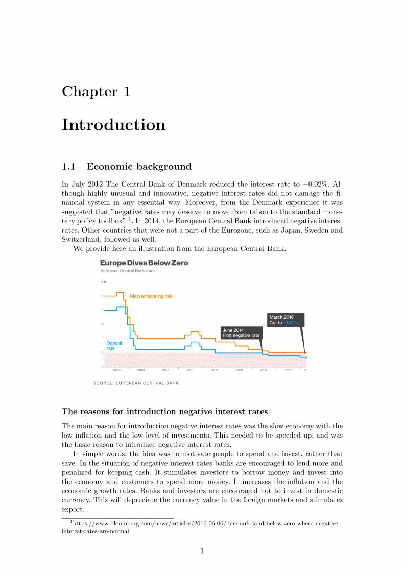
In July 2012 The Central Bank of Denmark reduced the interest rate to −0.02%. Al-though highly unusual and innovative, negative interest rates did not damage the fi-nancial system in any essential way. Moreover, from the Denmark experience it wassuggested that ”negative rates may deserve to move from taboo to the standard mone-tary policy toolbox” 1. In 2014, the European Central Bank introduced negative interestrates. Other countries that were not a part of the Eurozone, such as Japan, Sweden andSwitzerland, followed as well.
We provide here an illustration from the European Central Bank.
The reasons for introduction negative interest rates
The main reason for introduction negative interest rates was the slow economy with thelow inflation and the low level of investments. This needed to be speeded up, and wasthe basic reason to introduce negative interest rates.
In simple words, the idea was to motivate people to spend and invest, rather thansave. In the situation of negative interest rates banks are encouraged to lend more andpenalized for keeping cash. It stimulates investors to borrow money and invest intothe economy and customers to spend more money. It increases the inflation and theeconomic growth rates. Banks and investors are encouraged not to invest in domesticcurrency. This will depreciate the currency value in the foreign markets and stimulatesexport.
1https://www.bloomberg.com/news/articles/2016-06-06/denmark-land-below-zero-where-negative-interest-rates-are-normal
1
2 Irina Shadrina — SABR Volatility Smile Interpolation
Possible negative consequences
We would like to discuss possible negative implications if the negative interest rates willstay on the market for a long time.
One of the first concerns that comes to mind is whether the low rates will cause thebubbles on the housing market.
Also, banks are encouraged to move from safe assets, like government bonds, to morerisky ones. This raises the financial stability risk and the risk of bank runs. Moreover,a possible result of that would by that the rules of banking capital requirements willimply the higher obligatory reserves.
Banks are not sure about the reaction of the depositors on the introduction of thenegative interest rates for their deposits and are afraid to lose customers. This can makethe banks less profitable. Lower profitability means lower earnings, and that will makeit harder for banks to build up capital during the next credit cycle. A notable exampleis described in the article ”In the era of negative interest rates, Japans second-largestbank finds itself having to run just to stand still.” 1
Negative interest rates put pressure profitability of insurers and pension companies.Negative interest rates reduce the discount on the cash flows from assets. The presentvalue of liabilities of the insurance companies and pension funds is getting bigger, andso do the computed reserves. Moreover, to keep reserves on a bank account, companieswould have to pay.
If negative interest rates stay for a substantially long period, financial institutionswill be forced to change their behaviour. This will cause additional risks and unknowneffects. Typical market behaviour could be changed as well.
If more countries will introduce negative interest rates, this will also diminish ex-pected positive effects for the economy of the countries that did this first. For instance,the currency depreciation would probably be turned back.
Expected timeframe for the existence of the negative interest rates
It is difficult to predict how long these low interest rates will stay, but it seems possiblethat they will be low for quite some time. This is certainly the view of financial markets,where the return on government bonds is negative for a range of countries, even at longmaturities. 2 For instance, most private-sector forecasters don not expect Denmarkscentral bank to return to the positive interest rates again before 2018, at the earliest. 3
End-customer perspective on negative interest rates
It was always believed that the interest rates could not go below zero. Indeed, people canalways withdraw cash and keep it outside the banking system (say, at home), earningthe zero interest rate.
Nowadays, we realize that the customers are ready to pay for their bank account:it is convenient to use and can be cheaper, than keep the financial means in cash athome. The extra costs occur since cash needs to be stored, secured and insured. Thus,it is natural to suppose that the negative interest rates are limited from below, sincea person or a company is able to choose to keep the money in cash, if it will be moreprofitable for them, taking into account all extra costs and risks mentioned above.
However, there are many reasons to pay for storing money on the bank account andso the idea of negative interest rate is something we have to get used to.
1https://www.bloomberg.com/news/articles/2017-05-31/japan-s-second-largest-bank-has-to-run-just-to-stand-still
2https://www.ecb.europa.eu/press/key/date/2016/html/sp160728.en.html3https://www.bloomberg.com/news/articles/2016-06-06/denmark-land-below-zero-where-negative-
interest-rates-are-normal
SABR Volatility Smile Interpolation — Irina Shadrina 3
1.2 Problem statement
When most of the popular risk or pricing models in finance were developed, the generalassumption that the interest rates can not go below zero was one of the basic requiredproperties. Indeed, this reflected the market situation of that time and the expectationsfor the future interest rates behaviour.
For instance, the lognormal distribution was often used in stochastic modelling as agood reflection of the dynamics of the interest rates, financial instrument (like stocks)and some interest rate derivatives. The advantages of the lognormal distribution in-cluded that it was asymmetric (skewed to the right) and could not go below zero.
This kind of models is not able to reflect the negative interest rates. They are notdefined in this case or give wrong results and predict the wrong dynamics. In order tocope with negative interest rates these models should be adapted or new models shouldbe considered.
For instance, the Black-76 model, typically used to price options and compute themarket implied volatilities, assumes that the underlying process follows lognormal dis-tribution and assigns zero probability to non-positive interest rates.
The SABR model, developed by Hagan et. al. Hagan et al. [2002], is popular in fi-nancial industry because of the availability of an analytic asymptotic implied volatilityformula. Practical applications of the SABR model include interpolation of volatilitysurfaces and the hedging of volatility risk. In its original formulation the model is notsuitable for applications in the case of negative interest rates. In order to adapt theSABR model to the situation of negative interest rates, the following models were pro-posed in the literature (see Antonov et al. [2015a], Antonov et al. [2015b]): the DisplacedSABR, the Free Boundary SABR, the Normal SABR, and the Mixture SABR.
The aim of this thesis is to compare these models in terms of the quality of thevolatility smile interpolation. To our best knowledge there are no recent works wherethese models are calibrated to the nowadays market data and compared in this context.
The research question is the following.
Which extension of the SABR model is the most suitable for modelling the volatilitysmile in the presence of negative interest rates?
In order to answer this question we formulate a number of subquestions to set upcomparison criteria. They are arranged below in two groups, one deals with the quality ofthe computational output, and the other one deals with the evaluation of the analyticalproperties of the models.
The quality of the computational output of the models
One of the most important criteria for evaluation of the quality of modelling the volatilitysmile is whether it fits the market data. We want to choose the model that provides theefficient interpolation of the volatility smile. Thus, our first subquestion is:
(1) Does the model has sufficient fit to the market data? In which circumstances /states of the market?
To model the volatility smile we implement the following procedure. First, we cal-ibrate the model parameters using the market data. Second, we model the volatilitysmile using the estimated parameters.
There are two possible ways for the parameter calibration.
The first one is to use the approximation formula for the implied Normal volatilityintroduced in Hagan et al. [2002]. In this case we use the market data of the impliedNormal volatility to calibrate the model parameters. Then we model the volatility smile
4 Irina Shadrina — SABR Volatility Smile Interpolation
with the formula mentioned above. In this thesis we refer to this method as Hagan’sapproach.
The second way is to use an analytical formula for option prices derived for themodel. In this case we calibrate the model parameters using the market data of optionprices (or compute the option prices from the market data of the implied volatility).Then we compute option prices using the analytical formula mentioned above. Afterthat we model the volatility smile inserting the normal volatility values from optionprices. In this thesis we refer to this method as Antonov’s approach (we call it like thatsince it the only way to use their analytical formulas).
Since there is a one-to-one correspondence between the implied volatility and theoption price, it is important that the computed option prices are consistent. Amongother properties, they should not permit arbitrage. Thus, our second subquestion is:
(2) Does the model have arbitrage in option prices?
For the practical implementation of the model, the consistency of parameters is suf-ficient. We suppose that someone calibrates the parameters of the model to the currentmarket data daily (or it could be the case that someone recalibrates just one parameter,keeping the rest fixed). In this case, we want to avoid jumps in the recalibrated modelparameters. The reason to avoid jumps is that they can cause the corresponding jumpsin the dependant risk metrics and/or option prices computed using the model. Thus,our third subquestion is:
(3) Does the model have consistent and stable parameters?
The other issue that we find important for practical implementation of the model isthe complexity of its implementation. The model which permits an easy implementa-tion and recalibration of parameters guarantees transparency and comparability of theresults. We want that the volatility smile modelled by the model will not substantiallydepend on the algorithm we choose for implementation.
Therefore, our fourth subquestion is:
(4) Is the calibration of parameters stable and simple enough? Is the model easy toimplement in a computer code? Are the computational costs relatively small?
Evaluation of the analytical properties of the models
The models that we use for the volatility smile modelling assume different behaviourof the underlying forward. It is important that the behaviour of the forward reflectsthe behaviour we observe on the market. This helps us to avoid the misspecification ofthe model. Unquestionably, in our analysis we have to take into account the change ofmeasure, since we model the forward rate behaviour under the risk-neutral measure andthe observed market behaviour corresponds to the real world measure. Still, there areproperties conserved by the change of measure.
Our fifth subquestion is:
(5) Do the properties of the forward under the model reflect the expected marketbehaviour?
We find important to pay attention in our analysis to the following aspects. Themodel has to be not over-parametrized. All other things being equal, the model withless parameters should be preferred. The model has to be not too complex. Otherwiseit can have difficulty with the analytical tractability.
Our next subquestion is:
SABR Volatility Smile Interpolation — Irina Shadrina 5
(6) Which model is less parametrized? Which model is the least complex one?
One of the applications of the SABR model is the hedge of the volatility risk. Itis important to pay attention to the possibility to implement the hedge in models wecompare.
Our last subquestion is:
(7) Which model is the most consistent in terms of the hedge purposes? Is the hedgeprocess for the model described in the literature?
1.3 Thesis outline
The thesis is organized as follows. In Chapter 2 we review some definitions related to thefixed income security market. In Chapter 3 we introduce the mathematical frameworkand notations. In Chapter 4 we introduce the concept of the implied volatility. First,we consider the fundamental models: the Black and the Bachelier ones. Further, wegive a definition of the implied volatility and discuss its properties. The Chapter 5 isdevoted to the SABR model. In Chapter 6 we introduce extensions of the SABR modeladapted to negative interest rates: the Displaced SABR, the Free Boundary SABR, theNormal SABR, and the Mixture SABR. Chapter 7 contains computational results forall models. We investigate which extension of the SABR model is the most suitable forthe modelling of the volatility smile. Chapter 8 is devoted to the conclusion.
Chapter 2
Interest rate derivatives
In this Chapter we introduce some definitions related to the fixed income security mar-ket. Our goal is to give a short recollection of the main concepts that we use throughoutthe thesis. For a detailed explanation we refer the reader to Veronesi [2010] and Hull[2011], which we follow below closely.
2.1 Market of interest rate derivatives
A derivative can be defined as a financial instrument whose value depends on the valueof other, in general more basic, variables, usually assets [Hull, 2011, p.1].
In the case of an interest rate derivative [Hull, 2011, p.648] the underlying basicvariable is an interest rate or a set of different interest rates. Here are some examplesof interest rate derivatives: interest rate swaps, forward rate agreements, swaptions,interest rate caps and floors. Interest rate derivatives are commonly used to hedgeagainst interest rate movements, or in order to reduce or increase the interest rateexposure.
The derivatives market is the financial market for derivatives. Interest rate deriva-tives are traded in Over-The-Counter (OTC) and exchange-traded markets. Over-the-counter (OTC) trading is done directly between two parties, as opposite to the exchangetrading, which occurs via exchanges. Products traded on the exchange market must bewell standardized. In the meanwhile, the OTC market does not have this limitation.The OTC derivatives market is significant in some asset classes, such as: interest rates,foreign exchange, stocks, and commodities. From our discussion above it is clear thatthe OTC derivatives are important for hedging purposes (to hedge against interest raterisk, for instance). They can also be used to increase or to refine holder’s risk profile,for portfolio immunization or for speculation.
The interest rate derivatives play an important role in the current economy. Theinterest rates derivatives market is the largest in the world. The Bank for InternationalSettlements estimates the notional amount of the OTC derivatives contracts outstandingin December 2016 by $483 trillions BIS Monetary and Economic Department [2017].Their gross market value (the cost of replacing all outstanding contracts at currentmarket prices) $15 trillion.Notional amount of the OTC interest rate derivatives wasestimated by $368 trillions at end of December 2016, op. cit. Interest rate swaps are thesingle largest segment in the OTC derivatives market. At the end of December 2016,they accounted for 57% of the notional amount of all outstanding OTC derivatives and59% of the total gross market value, op. cit.
2.2 Interest rates
A discount factor [Veronesi, 2010, p.30] is the factor by which a future cash flow mustbe multiplied in order to obtain the present value. We determine the discount factor
6
SABR Volatility Smile Interpolation — Irina Shadrina 7
between two dates t and T as Z(t, T ).Interest rates [Veronesi, 2010, p.32] are closely related to discount factors, but are
more similar to the concept of return on an investment. The interest rate is the per-centage on the amount of money that a borrower promises to pay the lender.
The compounding frequency of the interest accruals refers to the number of timeswithin a year in which the interests are paid on the invested capital. For a given payoff,a higher compounding frequency results in a lower interest rate:
Payoff = P (1 +rn(t, T )
n)n,
where P is the value of the principal, and rn(t, T ) is the annualized n-times compoundedinterest rate, defined at time t for the future period T .
The continuously compounded interest rate is obtained by increasing the compound-ing frequency n to infinity.
limn→∞
(1 +rn(t, T )
n)n(T−t) = eR(t,T )(T−t)
The continuously compounded interest rate R(t, T ) is related with the n-times com-pounded interest rate rn(t, T ) by the following formula:
R(t, T ) = n log(1 +rn(t, T )
n).
People usually think of continuous compounding as daily compounding, since thereis no substantial difference between the daily compounded interest and the rate obtainedwith higher frequency.
Let us recall some standard interest rates available on the market. The LondonInterbank Offered Rate (LIBOR) [Hull, 2011, p.76] is produced daily by the Associationof British Banks, and it reflect the average of the interest rates estimated by the leadingbanks in London. It is an index that measures the cost of funds to large global banksoperating in London financial markets. The Euro Interbank Offered Rate (EURIBOR)is a daily reference rate, published by the European Money Markets Institute, based onthe averaged interest rates at which the banks in the Eurozone offer to lend unsecuredfunds to other banks.
The forward rate [Hull, 2011, p.84] is the rate of interest for the future period oftime, based on the today’s interest rates. To compute it from the given yield curve wecan use the no-arbitrage argument. It is applied in the following way. Suppose we havetwo historical continuously compounded interest rates r1 = r(t, T1) and r2 = r(t, T2),defined at the moment t, where t < T1 < T2 are the parameters for the starting andending moments for the action of these interest rates. To compute the value of thecontinuously compounded forward rate f := f(t, T1, T2) we use the equation
e−r2·(T2−t) = e−r1·(T1−t) · e−f ·(T2−T1).
Thus, for t = 0 we obtain
f(0, T1, T2) =r2T2 − r1T1T2 − T1
.
2.3 Interest rate derivatives
The Forward Rate Agreement (FRA) [Veronesi, 2010, p.162] is a contract in which oneparty pays the forward rate f(0, T1, T2) during a given future period from T1 to T2. Theother pays future market floating rate rn(T1, T2).
A forward contract [Veronesi, 2010, p.168] is a contract in which one party agrees tobuy and the other agrees to sell a given security at a given future time and at a givenprice, called the forward price.
8 Irina Shadrina — SABR Volatility Smile Interpolation
A plain vanilla fixed-for-floating interest rate swap contract [Veronesi, 2010, p.172]is an agreement in which:
• One party makes n fixed payments per year at an (annualized) rate s (the swaprate) on a notional N up to date T (tenor);
• The other party makes payments linked to a floating rate index rn(t) (typicallyLIBOR).
Denote by T1, T2, . . . , TM the payment days, ∆ = Ti − Ti−1 with ∆ = 1n . The net
payment at each of these days is computed in the following way:
Net payment at Ti = N ×∆× [rn(0, Ti−1)− s].
Cash flows correspond to long position in floating rate bond, and short position incoupon bond. No-arbitrage swap rate could be computed by the formula:
s = n× 1− Z(0, T )∑Mj=1 Z(0, Ti)
,
here T is the tenor of swap (duration of swap), Ti - payments dates, n - number ofpayments per year. A fixed-for-floating swap does not cost anything to enter, but canchange the duration of a portfolio.
The swap curve [Veronesi, 2010, p.177] at time t is the set of swap rates for allmaturities.
Futures and forward contracts [Veronesi, 2010, p.25] are contracts where two partiesagree to exchange a security (or cash, or a commodity) at a fixed time in the future fora price agreed today. Futures are traded on regulated exchanges. Forwards are tradedon the over-the-counter (OTC) market. A forward swap contract [Veronesi, 2010, p.179]means that two parties agree to enter into a fixed swap contract at a fixed future dateand for a fixed forward swap rate.
A call or put option [Veronesi, 2010, p.25] is a contract which gives the holder theright, but not the obligation, to buy or sell an underlying asset at a fixed strike price ona fixed date (maturity). Intuitively, an option is the financial equivalent of an insurancecontract.
A swaption [Veronesi, 2010, p.211] is the option on a swap rate. A swaption isAt-the-money (ATM) if the forward swap rate is (approximately) equal to the strike.
An interest rate cap [Veronesi, 2010, p.665] is a contract that pays the differencebetween LIBOR and a fixed rate, if this difference is positive, otherwise it pays zero. Itlooks like series of call options on the LIBOR rate. The cap insures a borrower with afloating-rate loan against increases in the LIBOR rate. A floor is exactly the reverse: aseries of put options on the LIBOR rate.

Chapter 3
Mathematical framework
In this Chapter we introduce some definitions related to the stochastic calculus. Thebasic reference for this Chapter is Etheridge [2002].
3.1 Assumptions
Before we introduce the main definitions and theorems important for our further work,we would like to mention the assumptions under which this theory was build up.
• The market is complete.
• No riskless arbitrage opportunity exists.
• Risk-free interest rate exists and is non-negative.
• It is possible to borrow and lend money at the same risk free interest rate.
• It is possible to sell (or buy) any quantity of any asset at any time.
• All securities are infinitely divisible.
• Short selling is allowed.
• There are no transaction costs.
• Underlying asset pays no dividends.
• You can buy and sell at the same time.
• Trading is continuous in time.
3.2 Ito calculus
The arbitrage [Etheridge, 2002, p.5] is the opportunity to earn a risk-free profit. Insimple words, there exists a trading strategy as follows: either we receive a positiveamount today and a non-negative tomorrow (with probability one) or we pay a zeroamount today and receive non-negative amount tomorrow (with a positive probabilityfor a positive profit).
A complete market [Etheridge, 2002, p.16] is the market where every contingentclaim can be replicated.
Statement (Law of One Price). [Veronesi, 2010, p.9] In the absence of arbitragetwo assets with the same payoff must have the same market price.
9
10 Irina Shadrina — SABR Volatility Smile Interpolation
The risk free rate is the rate of interest that can be earned in the absence of anyrisks (for instance, no risk of default, no reinvestment risk). The risk-free rate playsan important role in the mathematical theory of asset pricing. In the past, the LIBORrates were used as the risk-free rates. However, under stressed market conditions LIBORturned out to be a weak proxy for the risk free rate. Therefore, nowadays the marketpractice is to discount with the overnight index swap (OIS) rates Hull and White [2013].In the negative interest rate environment the suitable proxy for the risk-free rate is stilla subject for discussion. We can use the negative value of OIS, set the risk-free interestrate equal to zero (since we can keep cash and earn approximately the zero risk freerate), take the average of the appropriate interest rates from the past, or choose anothercurrency where the interest rates are positive (USD, for instance). As we can see, if weassume the negative value for the risk-free interest rate, we can create the arbitrageopportunity just by keeping money in cash, which is not consistent with our theory.Thus the fact that negative risk free rates are possible could only be explained withproperties not included in our model, such as the cost of saving cash or the fact thatthere is no risk-free asset in the real market.
We consider the probability space Haugh [2010] (Ω,F , P ). Here P is the real worldprobability measure, Ω is the universe of possible outcomes, the σ-algebra F representsthe set of possible events where an event is a subset of Ω. A filtration Ftt≥0 reflectsthe evolution of the information throughout time. For example, if at the moment t wealready know whether the event A happened, we assume that A ∈ Ft.
The Brownian motion Haugh [2010] Wt, t ≥ 0 is a stochastic process, such that
• W0 = 0,
• Wt is almost surely continuous,
• Wt has independent increments,
• Wt −Ws ∼ N (0, t− s) for 0 ≤ s ≤ t.
Note that Wt is almost surely nowhere differentiable.
The filtration Ft considered in this thesis is generated by the Brownian motionthat is specified in the model description.
A stochastic process Xt, t ≥ 0 is called martingale [Etheridge, 2002, p.33] withrespect to the filtration Ft and probability measure P if
EP [|Xt|] <∞ for all t ≥ 0 and EP [Xt+s|Ft] = Xt for all t, s ≥ 0
A stochastic differential equation [Etheridge, 2002, p.91] is an equation of the fol-lowing form:
dXt = µ(t,Xt)dt+ σ(t,Xt)dWt.
Here µ(t,Xt) is predictable and (Lebesgue) integrable function, and σ(t,Xt) is Ito-integrable function. They satisfy
∫ t0 (σ2s + |µ2s|)ds <∞.
An Ito-process Haugh [2010] is a solution of a stochastic differential equation. It canbe expressed as the sum of an integral with respect to the Brownian motion and anintegral with respect to time:
Xt = X0 +
∫ t
0µ(s,Xs)ds+
∫ t
0σ(s,Xs)dWs.
We proof the property of the sum of two uncorrelated Brownian motions with thezero-drift. This property we will use in the Chapter 9 of this thesis.
SABR Volatility Smile Interpolation — Irina Shadrina 11
Lemma 1 (Ito’s Lemma). Haugh [2010] Suppose f(t, x) is a twice continuouslydifferentiable function on R. Consider the Ito process dXt = µ(t,Xt)dt + σ(t,Xt)dWt.Then the process Zt := f(t,Xt) satisfies the following stochastic equation:
dZt =∂f
∂t(t,Xt)dt+
∂f
∂x(t,Xt)dXt +
1
2
∂2f
∂x2(t,Xt)(dXt)
2
= (∂f
∂t(t,Xt) +
∂f
∂x(t,Xt)µ(t,Xt) +
1
2
∂2f
∂x2(t,Xt)σ
2(t,Xt))dt+∂f
∂x(t,Xt)σ(t,Xt)dWt.
Theorem 1 (Fokker-Planck (the forward Kolmogorov) equation). [Gardiner,2004, p.138] The probability density function p(t, x) of a stochastic Ito-process dXt =µ(t,Xt)dt+ σ(t,Xt)dWt satisfies the following equation:
∂
∂tp(t, x) = − ∂
∂x[µ(t, x)p(t, x)] +
1
2
∂2
∂x2[σ2(t, x)p(t, x)].
Theorem 2 (Martingale representation theorem). [Etheridge, 2002, p.100] LetWt be the standard Brownian motion with a filtration Ft. If Mt is a martingale, adaptedto Ft and E[M2
t ] < ∞, then there exists a unique Ft-predictable stochastic process Ctsuch that
dMt = CtdWt.
The coefficient Ct may be deterministic or random, and may depend on any infor-mation that is available at time t.
3.3 Pricing under the risk neutral measure
A Risk-neutral probability measure (or an equivalent martingale measure) is a probabilitymeasure Q such that the discounted price of the derivative process is martingale.
As we can see, under the risk-neutral measure the derivative earns risk-free interestrate. Under this measure the derivative price (with no intermediate payments) can becomputed as the discounted value of its expected payoff at the payment day.
Theorem 3. Haugh [2005] The market is free of arbitrage and complete if and only ifthere exists a risk-neutral probability measure Q equivalent to the real world measure Psuch that the discounted price process St/Bt is a martingale. Here we denote by St theprice process of a risky asset, and by Bt the price process of a risk-free asset.
We can price financial derivatives under the risk-neutral measure using the followingformula:
V (0, T ) = e−rT × (expected payoff at T, computed under Q).
Risk-neutral density-based tests
Here we present a no-arbitrage test and some tests for the existence of the risk-neutraldensity, discussed in the literature Breeden and Litzenberger [1978]. These tests areused to check whether the model is consistent.
• Put-Call parity must be satisfied.
• The implied risk-neutral probability density function is integrated to one.
• The implied risk-neutral probability density function is positive.
• The risk-neutral density function produces call prices decreasing monotonicallywith respect to the strike.
12 Irina Shadrina — SABR Volatility Smile Interpolation
The risk-neutral market implied probability density function can be computed as thesecond order derivative of the call option price with respect to the strike Breeden andLitzenberger [1978]. The value at a price x of the discounted risk neutral density fST (x)is the second partial derivative of the call price with respect to the strike, evaluated atx:
e−rT fST (x) =∂2
∂K2C(K,T )|K=x.
Chapter 4
Implied volatility
In this Chapter we introduce the conception of implied volatility. First, the fundamentalmodels: the Black and the Bachelier models are examined. These models assume thatthe underlying forward rate follows the lognormal and the normal process, respectively,with a constant volatility and a constant risk-free rate. Further, we give the definitionof the implied volatility and discuss their properties.
4.1 Black’s model
The market standard for quoting option prices is Black’s model, developed by FischerBlack in 1976. This variant of the BlackScholes option pricing model is usually used toprice options on interest rate caps and floors or swaptions. The Black’s model assumesthat a forward rate Ft (for instance the LIBOR forward or a forward swap rate) followsa driftless lognormal process.
Namely, in Black’s model the forward rate is modelled under the risk-neutral measureby the following dynamics:
dFt = σBFtdWt,
F (0) = F0.
The parameter σB is called the Black volatility. This stochastic equation has the follow-ing solution: F = F0 × exp(−1
2σ2t+ σWt). As we can see from this solution, the values
of the forward rate F are always positive for F0 > 0.
The price of the call option with the maturity T and the strike K under this modelis given by:
V Bcall = e−rT [F0N(d1)−KN(d2)],
where
d1 =log(F0/K) + (σ2B/2)T
σ√T
,
d2 = d1 − σ√T ,
N(·) is the cumulative normal distribution and r is the risk-free rate.
4.2 Bachelier’s model
European option prices are often quoted by using the Normal (Bachelier) model. In thismodel the forward asset price Ft follows the following dynamics:
dFt = σNdWt,
13
14 Irina Shadrina — SABR Volatility Smile Interpolation
where F (0) = F0. The parameter σN is called the normal volatility. This stochasticequation has the following solution: F (t) = F0 +σNW (t). The price of the option underthis model is:
V Ncall = e−rT [(F0 −K)N(d1) +
σN√T√
2πe−d
21/2],
where d1 = F0−KσN√T
.
Note that the formula for options prices contains only the difference between thestrike and the initial forward value. Thus, if we shift a both on the same shift parameters we obtain the same option price under this model (the price does not depends on theshift value).
4.3 Implied volatility
To find the implied volatility we solve the equation for σ, using the market data for theoption price:
Price(r, T, σ, F0) = Market price.
The option value under the Black or Bachelier model is the increasing function ofσ. Thus we can find the unique solution of the equation:
σimpl = f(r, T, F0,Market price),
where σimp is the implied volatility.There is no analytical solution for this equation but we can use numerical methods
to find the approximate value of σimp.European option prices are often quoted by using the Normal (Bachelier) or the
Black model. The values of the implied volatility are given as annualized percentages:
volatility = 100× σimp ×√
250%
4.4 Comparison of Normal and Black volatilities
Implied lognormal volatility is measured by the relative changes of the forward rate.On the contrary, the Normal model measures the implied normal volatility in absolutechanges of the forward rate. Thus it makes more sense to compare implied normalvolatilities with historical moves of the underlying forward rate.
The Black model does not permit the process to go below zero, thus the impliedBlack volatility is determined only for positive values of the forward rate. It is possible tocompute the shifted lognormal implied volatility in the case of negative or zero forwards.In this case, the value of the shifted lognormal volatility depends on the value of theshift parameter. Under the Normal model there is non-zero probability for forward rateto be negative. One of the disadvantages of the Normal model is that extreme negativevalues are possible (though with small probability).
The normal model seems to capture the rates dynamics better than the lognormalmodel Hohmann et al. [2015].
Since both volatilities are determined from the formulas
PriceBlack(r, T, σB, F0) = PriceNormal(r, T, σN , F0) = Market price,
there is a one-to-one relation between the implied Black and the implied Normal volatil-ities. Usually, we can approximately express one through the other. For instance, in thecase of swaption pricing we have the following relationship between the volatilities forthe ATM swaptions Hohmann et al. [2015]:
σB ≈σNdF
.
SABR Volatility Smile Interpolation — Irina Shadrina 15
This approximation is less accurate in the case of low interest rates, when F is close tozero.
In the case of risk-neutral modelling the Normal volatility has advantages comparedto the Black volatility Hohmann et al. [2015].
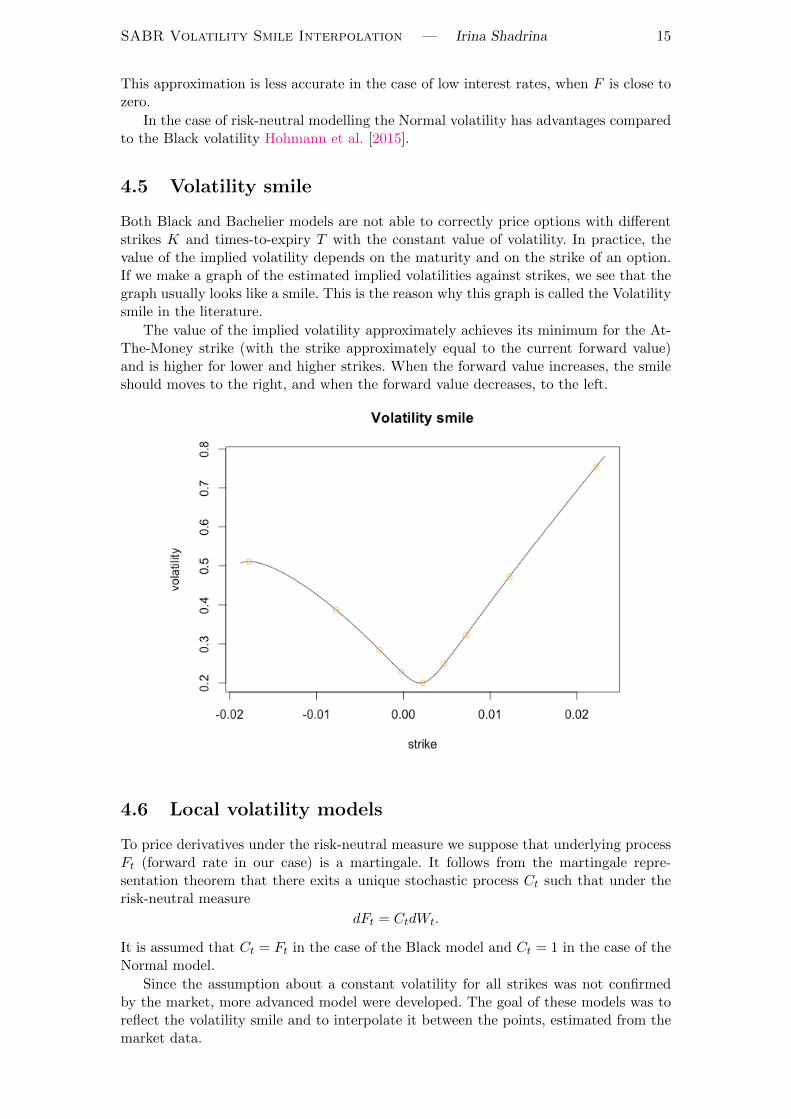
4.5 Volatility smile
Both Black and Bachelier models are not able to correctly price options with differentstrikes K and times-to-expiry T with the constant value of volatility. In practice, thevalue of the implied volatility depends on the maturity and on the strike of an option.If we make a graph of the estimated implied volatilities against strikes, we see that thegraph usually looks like a smile. This is the reason why this graph is called the Volatilitysmile in the literature.
The value of the implied volatility approximately achieves its minimum for the At-The-Money strike (with the strike approximately equal to the current forward value)and is higher for lower and higher strikes. When the forward value increases, the smileshould moves to the right, and when the forward value decreases, to the left.
4.6 Local volatility models
To price derivatives under the risk-neutral measure we suppose that underlying processFt (forward rate in our case) is a martingale. It follows from the martingale repre-sentation theorem that there exits a unique stochastic process Ct such that under therisk-neutral measure
dFt = CtdWt.
It is assumed that Ct = Ft in the case of the Black model and Ct = 1 in the case of theNormal model.
Since the assumption about a constant volatility for all strikes was not confirmedby the market, more advanced model were developed. The goal of these models was toreflect the volatility smile and to interpolate it between the points, estimated from themarket data.
16 Irina Shadrina — SABR Volatility Smile Interpolation
One of extensions of the Black model is a class of models called local volatilitymodels. Local volatility models are specified by assuming that Ct is a function of t andFt. The stochastic process Ft follows the following stochastic equation:
dFt = C(t, F (t))dWt,
where C(t, F ) is an instantaneous volatility.Local volatility models give correct option prices but predict wrong dynamics. Namely,
when the forward F (0) = f increases, the volatility curve shifts to left Hagan et al.[2002], which does not reflect the typical market behaviour. This property causes prob-lems by hedging.
Constant Elasticity of Variance (CEV) model
The CEV model is one of the Local volatility models. The forward rate has the followingdynamics:
dFt = σF βt dWt,
where σ is a positive constant and β ∈ [0, 1].There is an analytical solution for the risk-neutral probability density function. An-
alytic pricing formulas for the CEV model in terms of Bessel function series have beenderived for any value of β, but these formulas are computationally intensive. There arealso various analytical approximations for the transition density function.
The transition probability density function can be found as a solution of the back-ward Kolmogorov equation with absorbing (for all values of β) or reflecting (for β ∈[12 , 1)) boundary conditions. The CEV process with the absorbing condition is a mar-tingale Antonov and Spector [2012].
Chapter 5
SABR model
In this Chapter we introduce the SABR (stochastic alpha, beta, rho) model, developedby Hagan et. al. and introduced in Hagan et al. [2002]. The SABR model is widely usedin the financial industry, especially in the interest rate derivative markets. The mostattractive properties of the model is that it captures the volatility smile and reflects thecorrect dynamics of the volatility smile. Moreover, there is a closed-form approximationformula for the Black and Normal implied volatilities, as a function of the SABR modelparameters.
5.1 Model definition
By comparison with the CEV model, the SABR model adds a new stochastic factor tothe dynamics of the forward rate. Namely, it assumes that the volatility parameter itselffollows a lognormal stochastic process.
The SABR model is specified under the risk-neutral probability measure by thefollowing system of stochastic differential equations:
dFt = αtC(Ft)dWt,
dαt = ναtdZt,
dWtdZt = ρdt,
F (0) = f, α(0) = α are the initial conditions.
Here
• C(x) is the local volatility function, defined for x > 0 and assumed to be positive,smooth, and integrable around zero Hagan et al. [2015, first draft in 2001],∫ K
0
du
C(u)<∞;
• F (0) = f > 0 is the currently observed forward rate;
• ν > 0 is the volatility-of-volatility (volvol) of the forward rate;
• α(0) = α > 0 is the initial value for αt;
• dWt and dZt are two ρ−correlated Brownian motions;
• ρ ∈ (−1, 1).
The processes αt and Ft are correlated. If Ft changes, then αt changes as well. Thischange is proportional to the correlation coefficient ρ between the Brownian motions.
17
18 Irina Shadrina — SABR Volatility Smile Interpolation
Two Brownian motions dWt and dZt are correlated. We can express the second process
dZt from the first one using the Choleski decomposition: dZt = ρdWt+√
(1− ρ2)dW (1)t ,
where dW(1)t and dWt are two uncorrelated Brownian motions. Therefore,
Ft = F0 + α0
∫ t
0C(Fs)dWs + νρ
∫ t
0αk
∫ s
0C(Fs)dWsdWk
+ ν√
1− ρ2∫ t
0C(Fs)
∫ s
0αkdW
(1)k dWs.
In order to determine the model we have to estimate 4 parameters (f, ν, α, ρ) andchoose the function C(F ). For the standard SABR model we set C(F ) = F β, whereβ ∈ [0, 1). In this case the model is defined by 5 parameters (α, β, ρ, ν, f).
5.2 Risk-neutral probability density function
To apply the risk-neutral pricing theory described in the Chapter 3 we suppose thatthere exists a risk-neutral measure, under which the stochastic process Ft is a martingale.Our goal is to find the risk-neutral probability density function corresponding to thestochastic process Ft.
Let us define the risk-neutral probability density function implied by the two-dimensional process Ft as in Hagan et al. [2002]:
p(t, f, α, T, F,A)dFdA
= P (F ′ < F (T ) < F ′ + dF,A < α(T ) < A+ dA)|F (t) = f, α(t) = α).
Here we suppose that the economy of the market is in state F (t) = f , α(t) = α.
If we find the probability density function, then the value of the European call optionat the maturity T is the expected payoff of the option:
V (T, T ) = (expected payoff op the option at T)
= EQ[|F (T )−K|+|F (t) = f, α(t) = α]
=
∫ ∞−∞
∫ ∞K
(F −K)p(t, f, α, T, F,A)dFdA
The function p(·) satisfies the two-dimensional Fokker-Planck (Kolmogorov forward)partial differential equation Hagan et al. [2002]:
pT =1
2A2[C2(F )p]FF + ρν[A2C(F )p]FA +
1
2ν2[A2p]AA,
for T > t with
p = δ(F − f)δ(A− α) at T = t.
There is no analytical solution of this equation in the general case. When the SABRmodel was introduced, the approximation formula for the implied Normal and Blackvolatilities were derived in Hagan et al. [2002]. The explicit solution in the particularcase of β = 0 (Normal SABR) was given in Antonov et al. [2015b]. The explicit solutionin the zero-correlated case was given in Antonov et al. [2013] together with the mappingtechnique to the general case.
Once we find the approximate (or explicit) solution we check whether it is satisfac-tory, in the following sense. We have to check, whether the process Ft defined by thedensity function is martingale. It is also important that no-arbitrage conditions are pre-served: the put-call parity is true, the implied risk neutral density function is integratedto one, and it is positive.
SABR Volatility Smile Interpolation — Irina Shadrina 19
5.3 Results of Hagan et. al.
The SABR model was introduced in 2002 by Hagan et. al. in Hagan et al. [2015, firstdraft in 2001]. In Hagan et al. [2002] the approximation formula for the implied Normaland Black volatilities in terms of the SABR parameters was computed.
Hagan et. al. find the approximated solution of the Kolmogorov forward equationmentioned above. They use the singular perturbation technique and the known solutionof the Kernel Heat equation. For the simplicity they expressed the implied Normal andBlack volatilities in terms of the SABR parameters.
They suppose that α2T << 1, ν2T << 1. They also suppose that the values off and K are close to each other. The authors suggest that under the typical marketconditions this values are small. Thus the approximation formula is the most efficientin the area around the ATM values with relatively small T and volatilities.
The following approximation formula for the Normal implied volatility in the SABRsetting is proposed by Hagan et. al. in Hagan et al. [2014] as the most robust one:
σN (K) ≈ α(f −K)∫ fK
dxC(x)
· ζ
ξ(ζ)[1 +
[gα2 +
1
4ρνα
C(f)− C(K)
f −K+ ν2
2− 3ρ2
24
]τex
],
where τex is the time to exercise, and
ζ :=ν
α
∫ f
K
dx
C(x),
ξ(ζ) := log
(√1− 2ρζ + ζ2 − ρ+ ζ
1− ρ
),
g :=
log
(√C(f)C(K)
∫ fK
dxC(x)
f−K
)(∫ f
KdxC(x)
)2The typical choice for the function C(F ) is C(F ) = F β. In this case we obtain the
following equations:
σN (K) ≈ α(1− β)(f −K)
f1−β −K1−β · ζ
ξ(ζ)[1 +
[gα2 +
1
4ρνα
fβ −Kβ
f −K+ ν2
2− 3ρ2
24
]τex
],
where τex is the time to exercise,
ζ =ν
α
f1−β −K1−β
1− β,
ξ(ζ) = log
(√1− 2ρζ + ζ2 − ρ+ ζ
1− ρ
),
g =(1− β)2
(f1−β −K1−β)2log
((fK)
β2f1−β −K1−β
(1− β)(f −K)
),
and
σATM (K) ≈ αfβ(1 +
[−β(2− β)
24
α2
f2−2β+
1
4
ρναβ
f1−β+
2− 3ρ2
24ν2]τex)
In their recent article Hagan et al. [2016] written in 2016, the authors improved theaccuracy of their approach. They introduce the boundary correction formula, that can
20 Irina Shadrina — SABR Volatility Smile Interpolation
be used for the Displaced SABR, for instance. If we assume that we have a barrier suchthat for the forward holds Ft ≥ Fmin, then we can correct the option price formula byadding an extra term:
Vcall(τex,K) = V Ncall(τex, f,K, σN )− V N
call(τex, f,−K + 2Fmin, σN )
They also provide the new method to estimate the option price values by numericallysolving the effective forward equation.
5.3.1 Impact of parameters
The parameter β represents the expectation of traders about the distribution of theforward rate. Setting β close to zero we get a model close to the stochastic Normalmodel. If we take β close to one we a model closer to the stochastic Lognormal model.The volatility smile shifts upwards if one decreases β and downwards if one increases β.Also β influences the curvature of the volatility smile. The higher is β, the flatter is theskew.
Note that β = 0 determines the stochastic Normal model, β = 12 gives the stochastic
CIR model, and β = 1 corresponds to the stochastic Lognormal model.The parameter ρ controls the rotation of the curve. If we increase the value of ρ the
curve turns counter clockwise around the ATM value.The parameter ν (volvol) is the volatility of volatility. It has impact on the smile
curvature. The growth of ν increases the smile effect and vice versa.The parameter α governs the vertical location of the smile. The increase of α leads
to an upward shift of the entire smile, while the decrease results in a downward shift.As we can see, the influence of the parameters α and β partly overlaps. Thus if we fixthe value of β and estimate the value of α further, the parameter α can compensate thedifference.
The Backbone is the curve that is traced out from the ATM volatility when theinitial forward value f changes. It depends almost entirely on the value of β. If we takeβ = 0 the curve move down exponentially by increasing the initial forward value. If wetake β = 1 it moves right through the line.
5.3.2 Problems with Hagan et. al. formula
The original SABR approximation formula (and its improved version as well) leads tonegative probability densities for low strikes. Thus, the resulting pricing is not arbitragefree. However, the exact probability density obtained by numerically solving the effectiveforward equation proposed in Hagan et al. [2016] is always positive.
The approximation quality declines with time. For instance, for maturities largerthan 1 year the approximation error can be higher than 1% or even more for the ATMvalues Antonov and Spector [2012].
In 2014 Hagan et. al. proposed in Hagan et al. [2014] the no-arbitrage technique toreconstruct the no-arbitrage probability density function. They suppose that possibleforward values are limited on [Fmin, Fmax] and put absorbing boundary conditions onthe bounds. The probability density function, which is guaranteed to be positive (andsatisfies no-arbitrage conditions), can be found by solving the effective forward equation.As soon as we solve it numerically, we can compute the option prices and find thecorresponding Normal implied volatility which is guaranteed to be arbitrage free.
5.4 Results of Antonov et. al.
Antonov et. al. in Antonov and Spector [2012] find the explicit solution for the zero-correlation case (ρ = 0). Using the mapping technique (similarly to Hagan et. al.), theypropose the mimicking approximation for the general case.
SABR Volatility Smile Interpolation — Irina Shadrina 21
They set the absorbing boundary condition at zero, which guarantees the processFt to be martingale.
5.5 Parameters calibration
The general idea is that we try to find the optimal values of parameters by minimizingthe differences between the market values and the values estimated by the model. Theobjective function is
minν,α,ρ,β
∑(σmarket − σHagan)2.
Here σmarket are the market implied normal volatilities and σHagan are the values com-puted in the model.
It is possible to use in the formula above a weighted sum and put more weight forthe values around ATM. Indeed, these values are the most important in the case ofswaption pricing.
5.5.1 Hagan’s formula
The most convenient way to calibrate the SABR model to the market data is to use theHagan’s approximation formula. The model’s parameters have the following restrictions:ρ ∈ [−1, 1], β ∈ [−1, 1), ν ≥ 0, α > 0.
In Hagan et al. [2002] the authors advise to fix te value of β before other parameterscalibration. Usually the value of β can be chosen from prior believes of the appropriatemodel. For instance, β = 1 determines the stochastic lognormal model (typically chosenfor FX option markets), β = 1
2 defines the stochastic CIR model (used for interest ratemarkets), and β = 0 means the stochastic normal model (used in the case of zero ornegative forwards) . Other way to estimate it, is to run the liner regression betweennatural logarithm of the observed ATM volatility and natural logarithm of the forward.The following relationship is approximately true:
log σATM ≈ logα− (1− β) log f.
Thus the value of β can be estimated from the value of the slope plus one. It followsfrom the parameters properties (see above), that the choice of β does not substantiallyaffect the shape of the smile curve.
Since the ATM values should be fitted perfectly the value of α could be find as thesolution of the cubic equation for α. The smallest positive real root of the equationbelow, solved for α should be taken:
σATM (K) ≈ αfβ(1 + [−β(2− β)
24
α2
f2−2β+
1
4
ρναβ
f1−β+
2− 3ρ2
24ν2]τex)
The objective function in this case is:
minν,ρ
∑(σmarket − σHagan(α(β, ρ, ν), β, ρ, ν))2.
The local Levenberg-Marquardt algorithm was recommended in Floc’h and Kennedy[2014] as a fast and effective local minimizer for parameters calibration. Since the localminimum is possible and different sets of parameters could lead to almost the samevolatility smile, the efficient initial guess is important. In Gauthier and Rivaille [2009]and Floc’h and Kennedy [2014] are suggested methods for computing the parameters.
22 Irina Shadrina — SABR Volatility Smile Interpolation
5.5.2 Antonov’s formula
It is possible to estimate the values of parameters using the explicit formula for the zerocorrelation case, introduced in Antonov and Spector [2012]. In this case the differencesbetween the options prices, computed by Antonov’s formula, and the market values ofoption prices should be minimized. It is computationally more time consuming, includesthe computation of two dimensional integral (or the use of its approximation formula)and the results can depends on the grids, used by discretezation.
5.5.3 Fit to the market
Then the SABR model was introduced in 2002 by Hagan and all. Hagan et al. [2002] itwas the following market situation: interest rates were significantly positive, the volatil-ities were on ”normal levels”, quotes were in log-normal volatility or premium. In thiscircumstances the model gave a reasonably good fit to the market observed volatilitystructure. In its original formulation the SABR model is not suitable for applications inthe case of negative/zero interest rates. Therefore, several modifications of this modelwere proposed in the literature: Displaced SABR, Normal SABR, Free Boundary SABR,Mixture SABR.
Chapter 6
SABR extensions for negativeinterest rates
As we mentioned in the previous chapter, the SABR model is defined for the positiveinterest rate environment. In order to adapt the SABR model to the situation of negativeinterest rates, the following models were proposed in the literature: the Displaced SABR,the Free Boundary SABR, the Normal SABR, and the Mixture SABR. In this Chapterwe introduce this models and discuss their analytical properties.
6.1 Displaced SABR
It is now commonly accepted that interest rates do not need to be strictly positive. Aswe discussed in the Introduction part, it seems to be natural to suppose that negativeinterest rates are limited from below on the negative side. Let us suppose that thegeneral qualitative properties of the forward rate distribution did not change, when thenegative interest rates were introduced in the market. Moreover, suppose we are ableto estimate the minimal possible negative value of the forward. In this case, the mostnatural solution would be if we just shift the dynamics in a way that the boundarymoves from zero to the minimum possible forward determined by the market.
The Displaced SABR model is similar to the classic SABR model apart from thefact that a shift parameter s is introduced in the stochastic process of the forward rate.We introduce the Displaced model as a change of variable F ′ = F + s for s > 0 in theoriginal SABR model. As we can see dF ′ = dF . That gives us the following system ofequation:
dFt = αt(Ft + s)βdWt,
dαt = ναtdZt,
dWtdZt = ρdt,
F (0) = f, α(0) = α
This is equivalent to the assumption the F ′ follows the usual SABR model, that is, thatF ′ satisfies the following system of stochastic equations:
dF ′t = αtF′βt dWt,
dαt = ναtdZt,
dWtdZt = ρdt,
F ′(0) = f + s > 0, α(0) = α
Thus we are able to use the ordinary SABR results for F ′. We use the original formulasgiven in the previous chapter, but apply the changes f → f + s and K → K + sin our computations. The function C(F ) is equal to (F + s)β in this case. Note that
23
24 Irina Shadrina — SABR Volatility Smile Interpolation
the Bachelier option pricing formula depends only on the difference between the initialforward f and the strike K. So the value of the shift is not relevant in the option pricescomputations. However, it has influence on the values of the implied normal volatilityvalues that we compute from the Displaced SABR model.
6.1.1 Advantages of the Displaced SABR model
This set-up of the model reflects the current beliefs about existing of the minimumnegative interest rate (the boundary from below on the negative side).
It is easy to transform the ordinary SABR model to the Displaced SABR model. Inthe Displaced SABR model, the arbitrage problem with the implied probability densityfunction are shifted from zero to −s (we typically see the arbitrage around zero forthe ordinary SABR). Thus we have no problems with the probability density functionaround zero.
6.1.2 Disadvantages of the Displaced SABR model
The main drawback of this model is that in the case when the interest rates go belows (the floor for the rate value), a recalibration of the model parameters is necessaryand can cause jumps in greeks and option values. Also, sometimes the Displaced SABRmodel does not attain certain market prices Antonov et al. [2015b].
6.2 Normal SABR
In order to set up the Normal SABR model we take β = 0 or, equivalently, the functionC ≡ 1 in the SABR model. Thus under the Normal SABR model the forward ratefollows the following stochastic process:
dFt = αtdWt,
dαt = ναtdZt,
dWtdZt = ρdt.
As we can see from the equations above, in the Normal SABR model the incrementsof the forward rate do not depend on its current value. Typically this does not reflectthe beliefs about the forward rates behaviour. Another disadvantage is that the ”real”risk-neutral distribution is probably not symmetric. Indeed, it is very improbable thatinterest rates ever become below −10%. Hence, this approach makes sense only for shorttime horizons.
6.2.1 Hagan’s approximation formula
As it is advised in Hagan et al. [2002], in order to obtain the approximation formula forthe implied Normal volatility we can set C(f) = 1 and assume the free boundary. TheHagan’s approximation formula then simplifies to:
σN (K) ≈ α ζ
ξ(ζ)
[1 + ν2
2− 3ρ2
24τex
],
where τex is the time to exercise, and
ζ =ν
α(f −K),
ξ(ζ) = log
(√1− 2ρζ + ζ2 − ρ+ ζ
1− ρ
).
In this case the At-The-Money volatility is given by
σATM (K) ≈ α(1 +2− 3ρ2
24ν2τex).
SABR Volatility Smile Interpolation — Irina Shadrina 25
6.2.2 Antonov’s explicit solution
In Antonov et al. [2015b] the explicit for the Normal SABR with the free boundary isgiven.
Vcall(T,K) = EQ[FT −K]
= |f −K|+ +V0π
∫ ∞s0
G(γ2T, s)
sinh s
√sinh2 s− (k − ρ cosh s)2ds,
where
cosh s0 =−ρk +
√k2 + ρ2
ρ2
k =K − fV0
+ ρ
V0 =α
ν
ρ =√
1− ρ2
G(t, s) = 2√
2e−
t8
t√
2πt
∫ ∞s
ue−u2
2t
√coshu cosh sdu
Antonov et. al. suggest that this solution guarantees the positivity of the impliedprobability density function and that it is integrated to one.
The function G(t, s) is a one dimensional integral. In Antonov et al. [2013] an ap-proximation for it was given by a closed formula.
G(t, s) =
√sinh s
se−
s2
2t− t
8 (R(t, s) + δR(t, s)),
where:
R(t, s) = 1 +3tg(s)
8s2− 5t2(−8s2 + 3g(s)2 + 24g(s))
128s4
+35t3(−40s2 + 3g(s)3 + 24g(s)2 + 120g(s))
1024s6
g(s) = s coth s− 1
δR(t, s) = et8 − 3072 + 384t+ 24t2 + t3
3072
6.2.3 Practical computations with Antonov’s formula
We face with the problem with the uncertainties of the type 0/0 and ∞/∞ in theimplementation of Antonov’s formula in the program code. To avoid it, we do thefollowing steps.
First, we rewrite
Vcall(T,K) = EQ[FT −K]
= |f −K|+ +V0π
∫ ∞s0
G(γ2T, s)
√1− (k − ρ cosh s)2
sinh2 sds.
Secondly, following advise of the authors given in Antonov et al. [2013] we replaceR(t, s) by its fourth-order expansion for small s as a square root expression in G(t, s)expression. We obtain the following expression for the small s case (which determinesthe around at-the-money area).
26 Irina Shadrina — SABR Volatility Smile Interpolation
R(t, s) ≈ 1 + (1/8)t+ (1/128)t2 + (1/3072)t3+
(−(1/120)t− (1/4032)t2 − (1/15360)t3)s2+
((1/1260)t+ (1/56320)t3 − (1/40320)t2)s4
G(t, s) ≈√
1 + s2/6 + s4/120 e−s2/(2t)(R(t, s) + δR(t, s)).
6.2.4 Advantages of the Normal SABR model
This model gives a relatively good approximation to the volatility smile with a smallnumber of parameters. It is arbitrage free, since an explicit solution exists Antonov et al.[2015b].
6.2.5 Disadvantages of the Normal SABR model
As we have already mentioned above, the main disadvantage of this model is that thedynamics of the forward is not really consistent with the observable market data.
6.3 Free Boundary SABR
In Antonov et al. [2015a] Antonov et. al. propose an extension of the SABR modelcalled the Free Boundary SABR. Under the Free Boundary SABR model the forwardrate follows the following system of stochastic equations:
dFt = αt|Ft|βdWt, (6.1)
dαt = ναtdZt,
dWtdZt = ρdt,
F (0) = f, α(0) = α
with β ∈ [0, 1/2). As we can see, we set C(F ) = |F |β in this case. The non-negativenessof the function C(F ) guarantees that the increments of the stochastic process Ft arealways well defined. This model does not assume boundary conditions for Ft.
6.3.1 Antonov’s solution
In the case of ρ = 0, the explicit solution was computed in Antonov et al. [2015a]. Thissolution involves the computation of a two-dimensional integral. In Antonov et al. [2013]an asymptotic expansion of the function G(t, s) is derived, which reduces the overallcomputation to a one-dimensional integral. In the general case the authors apply theMarkovian projection to approximate this model by means of a projection onto the zerocorrelation case.
In Antonov et al. [2015a] authors determine the probability density function for theFree Boundary SABR model in terms of the Free Boundary CEV model. As a solutionfor the Fokker-Planck equation, the CEV probability density consists of two terms:the absorbing at zero solution and the reflecting at zero solution. Namely, p(t, f) =12(pR(t, |f |) + sign(f)pA(t, |f |). Since one of these two densities is singular at zero, weobserve the singularity around zero in the full density. In particular, the probabilitydensity function of the Free Boundary SABR model has two maxima. One of thesemaxima occurs exactly at F = 0. This singularity at F = 0 means a high probabilitythat the forward attains this value. This stickiness at zero has the consequence thatzero acts as an attractor of Monte-Carlo paths.
SABR Volatility Smile Interpolation — Irina Shadrina 27
6.3.2 Hagan’s approximation formula
For our computations we use the expression of the normal implied volatility obtainedfrom the Hagan’s approximation formula Hagan et al. [2014] by setting C(F ) = |F |β,as it was advised in Kienitz [2015].
σN (K) ≈ α(f −K)∫ fK
dx|x|β
· ζ
ξ(ζ)·
[1 +
[−β(2− β)
24|fK|β−1sgn(fK)α2 +
1
4ρνα|f |β − |K|β
f −K+ ν2
2− 3ρ2
24
]τex
],
where τex is the time to exercise, and
ζ =ν
α
∫ f
K
dx
|x|β,
ξ(ζ) = log
(√1− 2ρζ + ζ2 − ρ+ ζ
1− ρ
),
and ∫ f
K=
dx
|x|β=
f|f |β −
K|K|β
1− β
Let us mention that in Hagan et al. [2002] it was assumed that C(x) is smooth,symmetric and integrable around zero function. The function |x|β is not differentiableat zero. Although we can approximate is with a sequence of functions that satisfy theconditions of Hagan et al. [2002] that differ from |x|β only on a small punctured intervalaround zero, whose length tends to zero.
The quality of the approximation formula for the case fK < 0 is very questionablefrom the theoretical point of view. In this case f and K are lying on different sides of 0.The function |F |β has singularity at zero. Therefore, it is not correct to use the Tailorexpansion to obtain the approximation formula for this case. Indeed, this formula isbased on the approximation of the analytically derived function
g(K) := log
∫ fK√C(f)C(K)
C(x) dx
f −K
· (∫ f
K
dx
C(x)
)−2
by the first term of its Taylor series, in the case C(x) := |x|β. But in this case (whenf and K are of different sign) the corresponding Taylor series does not converge, so itsfirst order approximation has nothing to do with the actual value of g at the point K.
6.3.3 The approximation formula for the At-The-Money volatility
For our computations we derive the At-The-Money volatility approximation separatelyfrom the general case to avoid the 0/0 and ∞/∞ uncertainties. In our derivation wefollow the steps proposed in Hagan et al. [2002] for the ordinary SABR model. TheATM volatility is computed for the case K = f . If we try to substitute K = f in ourformula, we obtain 0/0 expressions. Thus we have to compute this case separately. Iff > 0, K > 0, we can use the usual Hagan’s approximation formula, see Chapter 4. So,here we assume that f < 0, K < 0.
Let us express f and K in the following way:
f = −elog(−f), K = −elog(−K).
28 Irina Shadrina — SABR Volatility Smile Interpolation
We obtain then the following expression:
f −K = −(elog(−f) − elog(−K)) =
= −e12log(−f)+ 1
2log(−K)(e
12log(−f)− 1
2log(−K) − e−(
12log(−f)− 1
2log(−K))) =
= −√fK(e
12log f
K − e−12log f
K ).
Then we use the expansion of sinhx = ex−e−x2 and obtain the following Taylor series
expansion for x = 12 log f
K :
f −K = −2√fK(
1
2log
f
K+
1
6(1
2log
f
K)3 +
1
120(1
2log
f
K)5 + . . . )
= −√fK log
f
K(1 +
1
24(log
f
K)2 +
1
1920(log
f
K)4 + . . . )
Following the same steps and taking the Tailor series expression for x = 12β log f
K :
(−f)β − (−K)β = β(fK)β2 log
f
K(1 +
1
24(β log
f
K)2 +
1
1920(β log
f
K)4 + . . . )
Thus we obtain the following expressions:
(−f)1−β − (−K)1−β = (1− β)(fK)1−β2 log
f
K(1 +
1
24(1− β)2(log
f
K)2+
1
1920(1− β)4(log
f
K)4 + . . . ).
and
(−f)β − (−K)β
f −K=β(fK)
β2 log f
K (1 + 124(β log f
K )2 + 11920(β log f
K )4 + . . . )
−√fK log f
K (1 + 124(log f
K )2 + 11920(log f
K )4 + . . . ).
Since we consider the case K = f we have log fK = 0. So, for f < 0, K < 0, the following
approximation is valid:(−f)β − (−K)β
f −K≈ −β|f |β−1.
In the case K = f the value of ζ is small and
χ(ζ) = ζ + o(ζ2).
Therefore, we have:ζ
χ(ζ)=
ζ
ζ + o(ζ2)≈ 1.
We substitute all expressions derived above in the main approximation formula forthe implied volatility and obtain the following final formula:
σATM ≈ α|f |β(1 + [−β(2− β)
24|f |2(β−1)α2 − 1
4ρναβ|f |β−1 +
2− 3ρ2
24ν2]τex)
As it was mentioned above, for the case f > 0, K > 0 we obtain the ordinary SABRformula for ATM volatility.
σATM (K) ≈ αfβ(1 +
[−β(2− β)
24
α2
f2−2β+
1
4
ρναβ
f1−β+
2− 3ρ2
24ν2]τex)
Thus we obtain the following final formula for the At-The-Money volatility:
σATM ≈ α|f |β(1 + [−β(2− β)
24|f |2(β−1)α2 +
1
4sgn(f)ρναβ|f |β−1 +
2− 3ρ2
24ν2]τex)
SABR Volatility Smile Interpolation — Irina Shadrina 29
6.3.4 Advantages of the Free Boundary SABR model
Negative forward rates are allowed. No extra parameter is needed by comparison withthe SABR model. The explicit solution exists in the zero correlation case.
6.3.5 Disadvantages of the Free Boundary SABR model
The model restricts the possible values for β ∈ [0, 12). In the original SABR model weallow β ∈ [0, 1). This limitation on β parameter means that models with propertiessimilar to the stochastic CIR model and stochastic lognormal model are not includedin the Free Boundary model. Although, in some circumstances this kind of models canreflect the market behaviour better.
Taking into account the stickiness of the risk-neutral density function at zero wecan suppose that the initial sign of the stochastic forward rate has influence on theinterest rate curve. Thus, in the case of implementing Monte Carlo simulations, theforward process with negative starting value predominantly stays on the negative sideand vice versa. This property could affect the hedging parameters. Probably, if we taketwo starting values with small differences but different sign, the options prices we obtainwill differ substantially. This can cause problems by hedging and affect the stability ofthe calibrated parameters.
6.4 Mixture SABR
The Mixture SABR model was introduced in Antonov et al. [2015b]. It is claimed tobe the more efficient in comparison with the previous models introduced above, for thefollowing reasons. This model can be solved exactly. It is arbitrage free. It has effect of”stickiness” near the zero forward rate (which reflects the observed market behaviourat that time).
In Antonov et al. [2015b] some analytical and computational research was done,though no explicit analytical formulas for the implied normal volatility, the probabilitydensity function and the price of the call option under this model were provided. In thischapter we derive explicit formulas for the implied volatility and option prices underthe Mixture model. Furthermore, we discuss some properties of the model that couldbe useful to make a decision whether this model is appropriate for the volatility smileinterpolation and option pricing.
6.4.1 Definition of Mixture SABR
The Mixture SABR was proposed first in Antonov et al. [2015b]. The goal was toneglect some drawbacks of the previous models, proposed and discussed in Antonovet al. [2015a].
Assume that the forward rate Ft can be written as
Ft = χF(1)t + (1− χ)F
(2)t ,
where
• F (1) follows a zero-correlation Free Boundary SABR model with the parameters(α1, β1, 0, ν1):
dF(1)t = α
(1)t |F
(1)t |β1dW
(1)t ,
dα(1)t = ν1α
(1)t dZ
(1)t ,
dW(1)t dZ
(1)t = 0
F (1)(0) = f, α(1)(0) = α1
30 Irina Shadrina — SABR Volatility Smile Interpolation
• F (2) follows a Normal SABR model with the parameters (α2, 0, ρ2, ν2),
dF(2)t = α
(2)t dW
(2)t ,
dα(2)t = ν2α
(2)t dZ
(2)t ,
dW(2)t dZ
(2)t = ρ2
F (1)(0) = f, α(2)(0) = α2
• χ is a random variable taking the value 1 with the probability p and 0 with theprobability 1− p.
We suppose that all Wiener processes are uncorrelated with each other and χ is
independent from F(1)t , F
(2)t , α
(1)t , α
(2)t .
This model is arbitrage free and permits negative interest rates Antonov et al. [2015b].It has closed-form solution for option prices and gives extra degrees of freedom becauseof new parameters. The model has 7 parameters (α1, α2, β1, ρ2, ν1, ν2, p) to be calibratedto market data.
Let us comment now on the parameter choices for the Mixture SABR. It is alwaysuseful to keep the same ATM volatility for both models Antonov et al. [2015b], leadingto the following relation of the initial stochastic volatility:
σ0 = α1Fβ10 = α2.
The value of p can be parametrized by an auxiliary parameter s via the followingformula given in Antonov et al. [2015b]:
p =σ0β1e
s
σ0β1es + |ν2ρ2|
.
This guarantees that the Mixture SABR model is reduced to either the zero-correlatedFree Boundary model or the Normal SABR model when ρ2 = 0 or β1 = 0, respectively.The probability parameter can be also used to control the singularity at zero. Namely,excluding it from the calibration parameters and setting it to small value reduces thesingularity arising from the zero-correlated Free Boundary model Antonov et al. [2015b].
In Antonov et al. [2015b] the following reduced parametrization set was proposed.
ν2 =ν1
1− β1
p =σ0β1
σ0β1 + |ν2ρ2|.
The reduced parametrization, proposed by the authors, increases the number ofparameters need to be calibrated to 4 parameters, like the original SABR model.
We would like to comment on the choice for p proposed by the authors.
We can rewrite the equation for p as:
p =1
1 + |ρ2ν2|β1σ0
, for σ0β1 6= 0.
For the case σ0 << 1 and 0 < β1 < 1/2 we obtain close to extreme choices for p:p ≈ 0 or p = 1.
SABR Volatility Smile Interpolation — Irina Shadrina 31
6.4.2 Analytical formulas for the Mixture SABR model
Probability density function, option prices
First, let us compute the distribution function of Ft. We use the independence of theunderlying stochastic processes and the random variable χ in our computation.
P (Ft ≤ x) = P (Ft ≤ x, χ ∈ 0, 1)
= P (χ = 1)P (F(1)t ≤ x) + P (χ = 0)P (F
(2)t ≤ x)
= pP (F(1)t ≤ x) + (1− p)P (F
(2)t ≤ x).
Thus, the cumulative distribution function of the Mixture model process is the weightedsum of the Normal model distribution functions and the Free Boundary distributionfunction.
We introduce the following notation:
• f1 is the probability density function of the zero-correlated Free SABR model;
• f2 is the probability density function of the Normal SABR model.
Then the probability density function of the Mixture model can be computed by thefollowing expression:
ft = (P (Ft ≤ x))′t = pf(1)t + (1− p)f (2)t .
Using these properties we can compute the call option price for the Mixture SABRmodel:
V callMixture = pV call
Zero Free Boundary + (1− p)V callNormal.
The explicit formulas for VZero Free Boundary and VNormal are given in Antonov et al.[2015b].
Martingale properties, no-arbitrage conditions
Below we show that the process Ft satisfies the no-arbitrage conditions. We assume
that the underlying processes F(1)t and F
(2)t satisfy the no-arbitrage conditions, as it
was mentioned in Antonov et al. [2015b].
We check the following properties of the probability density function of the stochasticprocess Ft:
1. Two underlying models (the zero-correlated Free Boundary SABR and the NormalSABR) have the same domain of definition, with the same σ-algebras, which allowsto consider their weighted sum.
2. Normalization:∫ +∞−∞ ft = p
∫ +∞−∞ f
(1)t + (1− p)
∫ +∞−∞ f
(2)t = 1.
3. Martingale property: E[FT ] = F0, since the processes F(1)t and F
(2)t are martin-
gales.
4. f ≥ 0 as a sum of two non-negative functions with positive weights: ft = pf(1)t +
(1− p)f (2)t .
32 Irina Shadrina — SABR Volatility Smile Interpolation
Implied normal volatility for the Mixture model
The value of the implied normal volatility under the Mixture model can be computedby the formula:
σNMixture =√p2σ2Zero Free Boundary + (1− p)2σ2Normal
Using the derivation of the approximation formulas for the Normal implied volatilityHagan et al. [2002] we find the implied normal volatilities for the underlying modelsthat satisfy the following equations:
dF(1)t ≈ σ(1)N dW
(1)t , F (1)(0) = f,
dF(2)t ≈ σ(2)N dW
(2)t , F (2)(0) = f.
Our goal is to find an approximation for σN such that
dFt ≈ σNdWt.
Let us define the process F′t = pF
(1)t + (1 − p)F (2)
t . This process F′t differs from Ft
but it has the same distribution function and density function as Ft. The option pricescomputed for these two processes are the same. Thus, we can conclude that σN = σ
′N
(this follows from the definition of the implied normal volatility). Here σ′N is determined
by the equation:
dF′t ≈ σ
′NdW
′t , F
′(0) = f.
Since F′
is the sum of two uncorrelated Ito’s processes, the variance of F′
and hence
the σN is equal to σN =
√p2σ
(1)2N + (1− p)2σ(2)2N .
The other way to determine the value of σN is to solve the equation Hagan et al.[2002]
V (τex, f) = p|f −K|
4√π
∫ ∞(f−K)2
2σ(1)2N
τex
e−q
q32
dq+(1−p) |f −K|4√π
∫ ∞(f−K)2
2σ(2)2N
τex
e−q
q32
dq =|f −K|
4√π
∫ ∞(f−K)2
2σ2Nτex
e−q
q32
dq
Then we solve the equation:
p
∫ ∞(f−K)2
2σ(1)2N
τex
e−q
q32
dq + (1− p)∫ ∞
(f−K)2
2σ(2)2N
τex
e−q
q32
dq =
∫ ∞(f−K)2
2σ2Nτex
e−q
q32
dq
This is equivalent to the following equation: Let us suppose that σ(1) ≤ σ(2) We cansee from the formula, that σN ∈ [σ(1), σ(2)]. Then we obtain the following formula
(1− p)∫ (f−K)2
2σ2Nτex
(f−K)2
2σ(2)2N
τex
e−q
q32
dq = p
∫ (f−K)2
2σ(1)2N
τex
(f−K)2
2σ2Nτex
e−q
q32
dq
Thus we see that σN can be characterized by the following property. The value (f −K)2/2σ2Nτex divides the segment [(f −K)2/2σ
(2)2N τex, (f −K)2/2σ
(2)2N τex] in such a way
that the square under the curve eq/q3/2 is divided in two parts with the proportionp/(1− p).
6.4.3 Advantages of the Mixture SABR model
The model has a closed-form solution and gives an extra degree of freedom because ofthe new parameter p.
SABR Volatility Smile Interpolation — Irina Shadrina 33
6.4.4 Disadvantages of the Mixture SABR model
The Mixture model can be seen as over-parametrized in comparison with the other mod-els described above. It is difficult to calibrate 6 parameters of the model simultaneously.The use of the restriction authors advise for the parameters, makes the model less un-derstandable from the practical point of view. There is no answer on the question ”Whywe mix the Normal and the Free Boundary models, except to the fact, that analyticalsolutions exist for both models?”.
The structure of the model can cause jumps in risk metrics and in Monte Carlosimulated paths because of the mixture structure.
Some general drawbacks of mixture-type models are discussed in Piterbarg [2003].We can apply the same arguments to the Mixture SABR model. Namely, it is notpossible to price path dependent derivatives using the mixture model, and there is alsoexplained a problem that occurs once one tries to apply a mixture models for hedging.
Chapter 7
Comparison of the models
In this Chapter we compare the models introduced in the previous Chapter. We as-sume that Ft is the stochastic process of the swap forward rate. Let us recall that weinvestigate which extension of the SABR model is the most suitable for the modellingof the volatility smile in the presence of negative interest rates. In order to answer thisquestion we formulate comparison criteria.
7.1 Comparison criteria
We aim to evaluate the models by the criteria, introduced in the Chapter 1. Let usbriefly recall them.
Computational: the quality of the fit (cf. the Subquestion (1) from the Introductionsection), the absence of arbitrage in the computed option prices (cf. the Sub-question (2)), the parameters consistency (cf. the Subquestion (3)), easiness ofimplementation and computational costs (cf. the Subquestion (4)).
Analytical: reflection of the analytical properties of the model in real market (cf. theSubquestion (5)); number of parameters of the model; existence intuitive expla-nation for models parameters; the complexity of the model (cf. the Subquestion(6)); hedging under the model (cf. the Subquestion (7)).
All other things being equal, the model with less parameters should be preferred. Ideally,we select the model that optimizes all our criteria with respect to the other models.
7.2 Market data
7.2.1 Implied normal volatility
For our analysis we use the data of the implied normal volatilities for the 6-monthsEURIBOR swaptions ranging from 1M X 2Y to 15Y x 30Y. We chose the followingtesting days: 04.11.2014, 01.07.2016, 03.01.2017, 15.03.2017, 30.05.2017, 31.05.2017. Wechoose a day with quite hight ATM (At-The-Money) value (04.11.2014), days withnegative ATM values and two days in a row to check the stability of parameters.
We observe different behaviour for the implied volatilities of swaptions with smallexpiry and maturity and swaption with long expiry and maturity. The volatility smilelooks more like a smile in the case of small expiry and maturity (less than 2 years). Thus,we observe the lower values for the implied volatilities around At-The-Money values. Ifthe distances between strikes and the At-The-Money value increase, then the values ofthe implied volatilities increase as well.
34
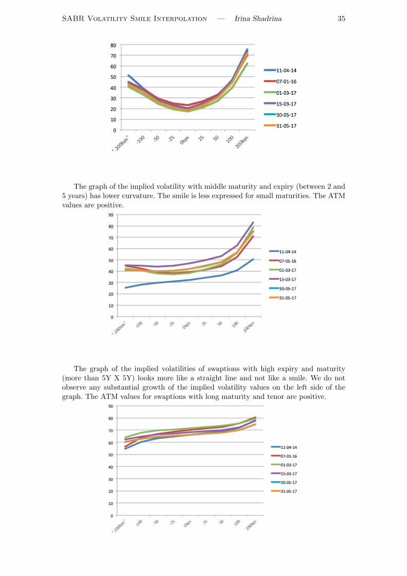
SABR Volatility Smile Interpolation — Irina Shadrina 35
The graph of the implied volatility with middle maturity and expiry (between 2 and5 years) has lower curvature. The smile is less expressed for small maturities. The ATMvalues are positive.
The graph of the implied volatilities of swaptions with high expiry and maturity(more than 5Y X 5Y) looks more like a straight line and not like a smile. We do notobserve any substantial growth of the implied volatility values on the left side of thegraph. The ATM values for swaptions with long maturity and tenor are positive.
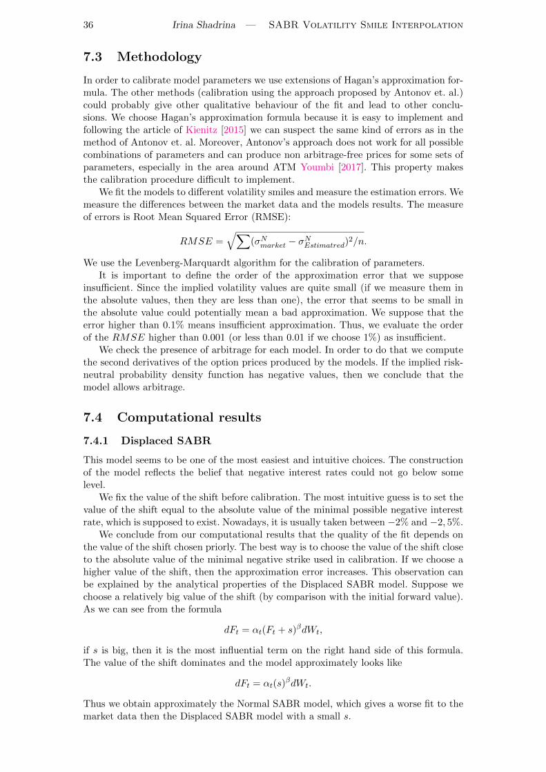
36 Irina Shadrina — SABR Volatility Smile Interpolation
7.3 Methodology
In order to calibrate model parameters we use extensions of Hagan’s approximation for-mula. The other methods (calibration using the approach proposed by Antonov et. al.)could probably give other qualitative behaviour of the fit and lead to other conclu-sions. We choose Hagan’s approximation formula because it is easy to implement andfollowing the article of Kienitz [2015] we can suspect the same kind of errors as in themethod of Antonov et. al. Moreover, Antonov’s approach does not work for all possiblecombinations of parameters and can produce non arbitrage-free prices for some sets ofparameters, especially in the area around ATM Youmbi [2017]. This property makesthe calibration procedure difficult to implement.
We fit the models to different volatility smiles and measure the estimation errors. Wemeasure the differences between the market data and the models results. The measureof errors is Root Mean Squared Error (RMSE):
RMSE =√∑
(σNmarket − σNEstimatred)2/n.
We use the Levenberg-Marquardt algorithm for the calibration of parameters.It is important to define the order of the approximation error that we suppose
insufficient. Since the implied volatility values are quite small (if we measure them inthe absolute values, then they are less than one), the error that seems to be small inthe absolute value could potentially mean a bad approximation. We suppose that theerror higher than 0.1% means insufficient approximation. Thus, we evaluate the orderof the RMSE higher than 0.001 (or less than 0.01 if we choose 1%) as insufficient.
We check the presence of arbitrage for each model. In order to do that we computethe second derivatives of the option prices produced by the models. If the implied risk-neutral probability density function has negative values, then we conclude that themodel allows arbitrage.
7.4 Computational results
7.4.1 Displaced SABR
This model seems to be one of the most easiest and intuitive choices. The constructionof the model reflects the belief that negative interest rates could not go below somelevel.
We fix the value of the shift before calibration. The most intuitive guess is to set thevalue of the shift equal to the absolute value of the minimal possible negative interestrate, which is supposed to exist. Nowadays, it is usually taken between −2% and −2, 5%.
We conclude from our computational results that the quality of the fit depends onthe value of the shift chosen priorly. The best way is to choose the value of the shift closeto the absolute value of the minimal negative strike used in calibration. If we choose ahigher value of the shift, then the approximation error increases. This observation canbe explained by the analytical properties of the Displaced SABR model. Suppose wechoose a relatively big value of the shift (by comparison with the initial forward value).As we can see from the formula
dFt = αt(Ft + s)βdWt,
if s is big, then it is the most influential term on the right hand side of this formula.The value of the shift dominates and the model approximately looks like
dFt = αt(s)βdWt.
Thus we obtain approximately the Normal SABR model, which gives a worse fit to themarket data then the Displaced SABR model with a small s.
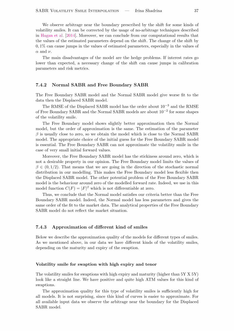
SABR Volatility Smile Interpolation — Irina Shadrina 37
We observe arbitrage near the boundary prescribed by the shift for some kinds ofvolatility smiles. It can be corrected by the usage of no-arbitrage techniques describedin Hagan et al. [2014]. Moreover, we can conclude from our computational results thatthe values of the estimated parameters depend on the shift. The change of the shift by0, 1% can cause jumps in the values of estimated parameters, especially in the values ofα and ν.
The main disadvantages of the model are the hedge problems. If interest rates golower than expected, a necessary change of the shift can cause jumps in calibrationparameters and risk metrics.
7.4.2 Normal SABR and Free Boundary SABR
The Free Boundary SABR model and the Normal SABR model give worse fit to thedata then the Displaced SABR model.
The RMSE of the Displaced SABR model has the order about 10−3 and the RMSEof Free Boundary SABR and the Normal SABR models are about 10−2 for some shapesof the volatility smile.
The Free Boundary model shows slightly better approximation then the Normalmodel, but the order of approximation is the same. The estimation of the parameterβ is usually close to zero, so we obtain the model which is close to the Normal SABRmodel. The appropriate choice of the initial guess for the Free Boundary SABR modelis essential. The Free Boundary SABR can not approximate the volatility smile in thecase of very small initial forward values.
Moreover, the Free Boundary SABR model has the stickiness around zero, which isnot a desirable property in our opinion. The Free Boundary model limits the values ofβ ∈ (0, 1/2). That means that we are going in the direction of the stochastic normaldistribution in our modelling. This makes the Free Boundary model less flexible thenthe Displaced SABR model. The other potential problem of the Free Boundary SABRmodel is the behaviour around zero of the modelled forward rate. Indeed, we use in thismodel function C(F ) = |F |β which is not differentiable at zero.
Thus, we conclude that the Normal model satisfies our criteria better than the FreeBoundary SABR model. Indeed, the Normal model has less parameters and gives thesame order of the fit to the market data. The analytical properties of the Free BoundarySABR model do not reflect the market situation.
7.4.3 Approximation of different kind of smiles
Below we describe the approximation quality of the models for different types of smiles.As we mentioned above, in our data we have different kinds of the volatility smiles,depending on the maturity and expiry of the swaption.
Volatility smile for swaption with high expiry and tenor
The volatility smiles for swaptions with high expiry and maturity (higher than 5Y X 5Y)look like a straight line. We have positive and quite high ATM values for this kind ofswaptions.
The approximation quality for this type of volatility smiles is sufficiently high forall models. It is not surprising, since this kind of curves is easier to approximate. Forall available input data we observe the arbitrage near the boundary for the DisplacedSABR model.
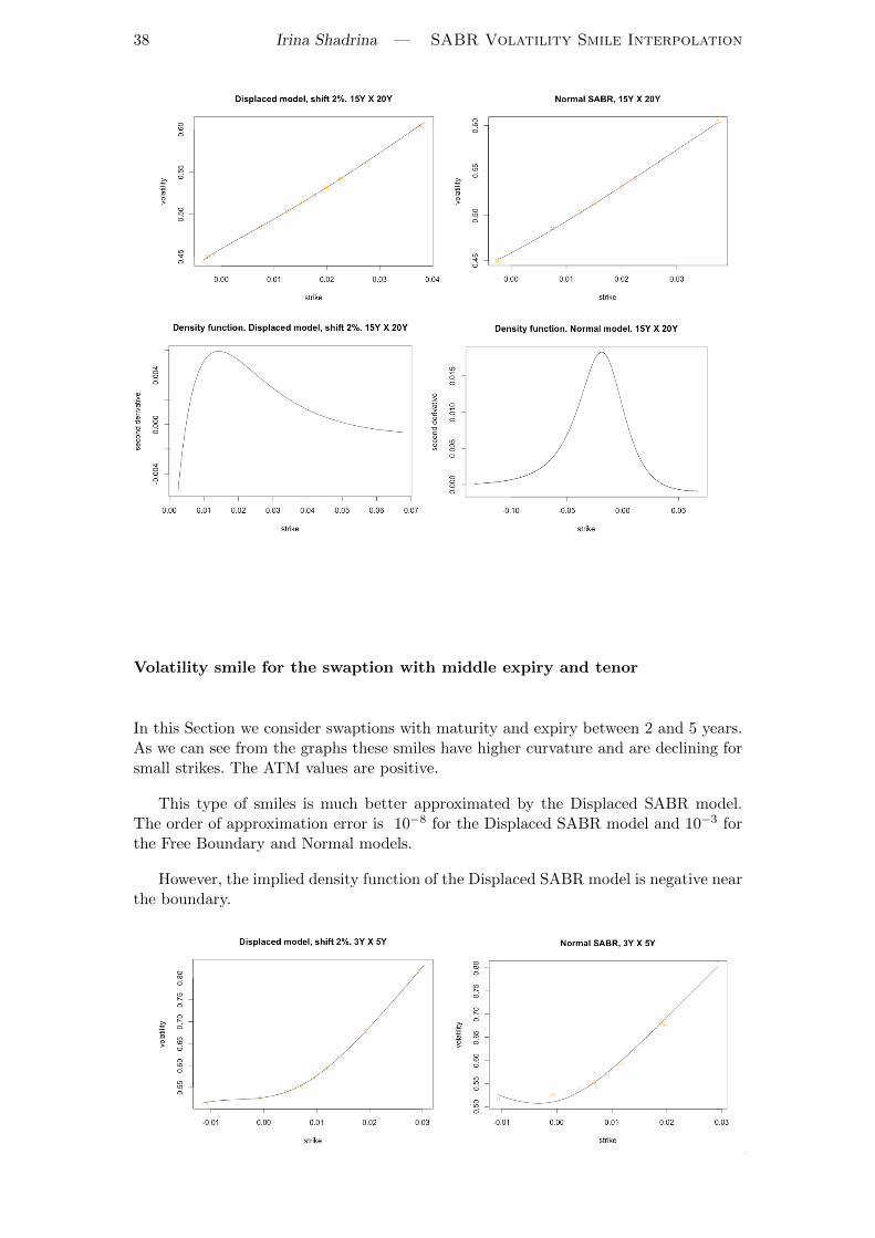
38 Irina Shadrina — SABR Volatility Smile Interpolation
Volatility smile for the swaption with middle expiry and tenor
In this Section we consider swaptions with maturity and expiry between 2 and 5 years.As we can see from the graphs these smiles have higher curvature and are declining forsmall strikes. The ATM values are positive.
This type of smiles is much better approximated by the Displaced SABR model.The order of approximation error is 10−8 for the Displaced SABR model and 10−3 forthe Free Boundary and Normal models.
However, the implied density function of the Displaced SABR model is negative nearthe boundary.
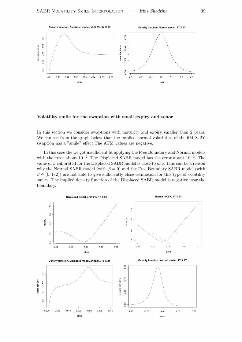
SABR Volatility Smile Interpolation — Irina Shadrina 39
Volatility smile for the swaption with small expiry and tenor
In this section we consider swaptions with maturity and expiry smaller than 2 years.We can see from the graph below that the implied normal volatilities of the 6M X 2Yswaption has a ”smile” effect.The ATM values are negative.
In this case the we got insufficient fit applying the Free Boundary and Normal modelswith the error about 10−2. The Displaced SABR model has the error about 10−3. Thevalue of β calibrated for the Displaced SABR model is close to one. This can be a reasonwhy the Normal SABR model (with β = 0) and the Free Boundary SABR model (withβ ∈ (0, 1/2)) are not able to give sufficiently close estimation for this type of volatilitysmiles. The implied density function of the Displaced SABR model is negative near theboundary.
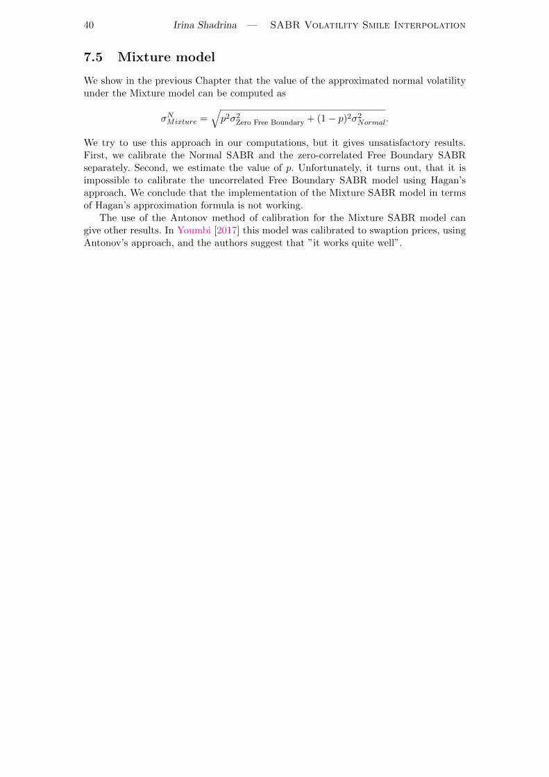
40 Irina Shadrina — SABR Volatility Smile Interpolation
7.5 Mixture model
We show in the previous Chapter that the value of the approximated normal volatilityunder the Mixture model can be computed as
σNMixture =√p2σ2Zero Free Boundary + (1− p)2σ2Normal.
We try to use this approach in our computations, but it gives unsatisfactory results.First, we calibrate the Normal SABR and the zero-correlated Free Boundary SABRseparately. Second, we estimate the value of p. Unfortunately, it turns out, that it isimpossible to calibrate the uncorrelated Free Boundary SABR model using Hagan’sapproach. We conclude that the implementation of the Mixture SABR model in termsof Hagan’s approximation formula is not working.
The use of the Antonov method of calibration for the Mixture SABR model cangive other results. In Youmbi [2017] this model was calibrated to swaption prices, usingAntonov’s approach, and the authors suggest that ”it works quite well”.
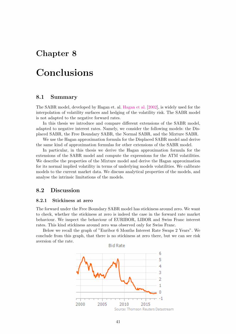
Chapter 8
Conclusions
8.1 Summary
The SABR model, developed by Hagan et. al. Hagan et al. [2002], is widely used for theinterpolation of volatility surfaces and hedging of the volatility risk. The SABR modelis not adapted to the negative forward rates.
In this thesis we introduce and compare different extensions of the SABR model,adapted to negative interest rates. Namely, we consider the following models: the Dis-placed SABR, the Free Boundary SABR, the Normal SABR, and the Mixture SABR.
We use the Hagan approximation formula for the Displaced SABR model and derivethe same kind of approximation formulas for other extensions of the SABR model.
In particular, in this thesis we derive the Hagan approximation formula for theextensions of the SABR model and compute the expressions for the ATM volatilities.We describe the properties of the Mixture model and derive the Hagan approximationfor its normal implied volatility in terms of underlying models volatilities. We calibratemodels to the current market data. We discuss analytical properties of the models, andanalyse the intrinsic limitations of the models.
8.2 Discussion
8.2.1 Stickiness at zero
The forward under the Free Boundary SABR model has stickiness around zero. We wantto check, whether the stickiness at zero is indeed the case in the forward rate marketbehaviour. We inspect the behaviour of EURIBOR, LIBOR and Swiss Franc interestrates. This kind stickiness around zero was observed only for Swiss Franc.
Below we recall the graph of ”Euribor 6 Months Interest Rate Swaps 2 Years”. Weconclude from this graph, that there is no stickiness at zero there, but we can see riskaversion of the rate.
41
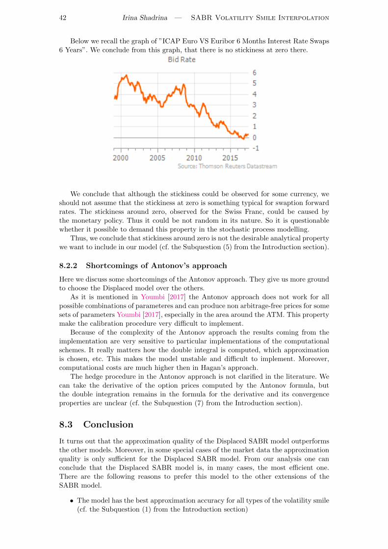
42 Irina Shadrina — SABR Volatility Smile Interpolation
Below we recall the graph of ”ICAP Euro VS Euribor 6 Months Interest Rate Swaps6 Years”. We conclude from this graph, that there is no stickiness at zero there.
We conclude that although the stickiness could be observed for some currency, weshould not assume that the stickiness at zero is something typical for swaption forwardrates. The stickiness around zero, observed for the Swiss Franc, could be caused bythe monetary policy. Thus it could be not random in its nature. So it is questionablewhether it possible to demand this property in the stochastic process modelling.
Thus, we conclude that stickiness around zero is not the desirable analytical propertywe want to include in our model (cf. the Subquestion (5) from the Introduction section).
8.2.2 Shortcomings of Antonov’s approach
Here we discuss some shortcomings of the Antonov approach. They give us more groundto choose the Displaced model over the others.
As it is mentioned in Youmbi [2017] the Antonov approach does not work for allpossible combinations of parameteres and can produce non arbitrage-free prices for somesets of parameters Youmbi [2017], especially in the area around the ATM. This propertymake the calibration procedure very difficult to implement.
Because of the complexity of the Antonov approach the results coming from theimplementation are very sensitive to particular implementations of the computationalschemes. It really matters how the double integral is computed, which approximationis chosen, etc. This makes the model unstable and difficult to implement. Moreover,computational costs are much higher then in Hagan’s approach.
The hedge procedure in the Antonov approach is not clarified in the literature. Wecan take the derivative of the option prices computed by the Antonov formula, butthe double integration remains in the formula for the derivative and its convergenceproperties are unclear (cf. the Subquestion (7) from the Introduction section).
8.3 Conclusion
It turns out that the approximation quality of the Displaced SABR model outperformsthe other models. Moreover, in some special cases of the market data the approximationquality is only sufficient for the Displaced SABR model. From our analysis one canconclude that the Displaced SABR model is, in many cases, the most efficient one.There are the following reasons to prefer this model to the other extensions of theSABR model.
• The model has the best approximation accuracy for all types of the volatility smile(cf. the Subquestion (1) from the Introduction section)
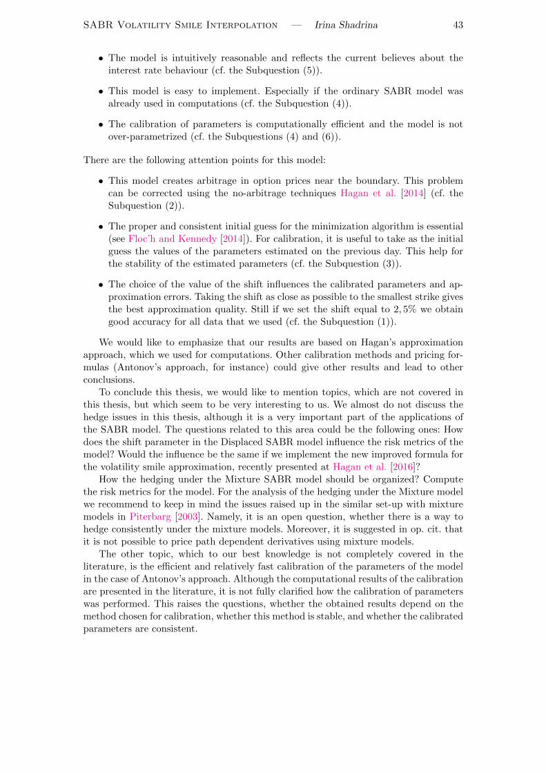
SABR Volatility Smile Interpolation — Irina Shadrina 43
• The model is intuitively reasonable and reflects the current believes about theinterest rate behaviour (cf. the Subquestion (5)).
• This model is easy to implement. Especially if the ordinary SABR model wasalready used in computations (cf. the Subquestion (4)).
• The calibration of parameters is computationally efficient and the model is notover-parametrized (cf. the Subquestions (4) and (6)).
There are the following attention points for this model:
• This model creates arbitrage in option prices near the boundary. This problemcan be corrected using the no-arbitrage techniques Hagan et al. [2014] (cf. theSubquestion (2)).
• The proper and consistent initial guess for the minimization algorithm is essential(see Floc’h and Kennedy [2014]). For calibration, it is useful to take as the initialguess the values of the parameters estimated on the previous day. This help forthe stability of the estimated parameters (cf. the Subquestion (3)).
• The choice of the value of the shift influences the calibrated parameters and ap-proximation errors. Taking the shift as close as possible to the smallest strike givesthe best approximation quality. Still if we set the shift equal to 2, 5% we obtaingood accuracy for all data that we used (cf. the Subquestion (1)).
We would like to emphasize that our results are based on Hagan’s approximationapproach, which we used for computations. Other calibration methods and pricing for-mulas (Antonov’s approach, for instance) could give other results and lead to otherconclusions.
To conclude this thesis, we would like to mention topics, which are not covered inthis thesis, but which seem to be very interesting to us. We almost do not discuss thehedge issues in this thesis, although it is a very important part of the applications ofthe SABR model. The questions related to this area could be the following ones: Howdoes the shift parameter in the Displaced SABR model influence the risk metrics of themodel? Would the influence be the same if we implement the new improved formula forthe volatility smile approximation, recently presented at Hagan et al. [2016]?
How the hedging under the Mixture SABR model should be organized? Computethe risk metrics for the model. For the analysis of the hedging under the Mixture modelwe recommend to keep in mind the issues raised up in the similar set-up with mixturemodels in Piterbarg [2003]. Namely, it is an open question, whether there is a way tohedge consistently under the mixture models. Moreover, it is suggested in op. cit. thatit is not possible to price path dependent derivatives using mixture models.
The other topic, which to our best knowledge is not completely covered in theliterature, is the efficient and relatively fast calibration of the parameters of the modelin the case of Antonov’s approach. Although the computational results of the calibrationare presented in the literature, it is not fully clarified how the calibration of parameterswas performed. This raises the questions, whether the obtained results depend on themethod chosen for calibration, whether this method is stable, and whether the calibratedparameters are consistent.
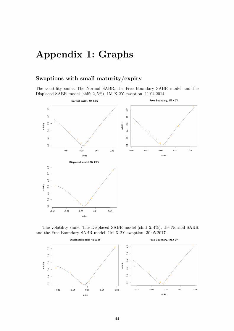
Appendix 1: Graphs
Swaptions with small maturity/expiry
The volatility smile. The Normal SABR, the Free Boundary SABR model and theDisplaced SABR model (shift 2, 5%). 1M X 2Y swaption. 11.04.2014.
The volatility smile. The Displaced SABR model (shift 2, 4%), the Normal SABRand the Free Boundary SABR model. 1M X 2Y swaption. 30.05.2017.
44
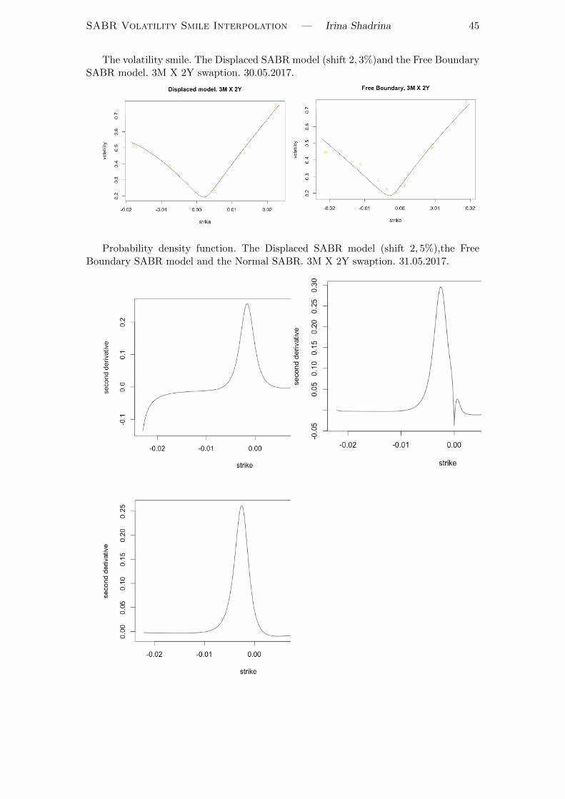
SABR Volatility Smile Interpolation — Irina Shadrina 45
The volatility smile. The Displaced SABR model (shift 2, 3%)and the Free BoundarySABR model. 3M X 2Y swaption. 30.05.2017.
Probability density function. The Displaced SABR model (shift 2, 5%),the FreeBoundary SABR model and the Normal SABR. 3M X 2Y swaption. 31.05.2017.
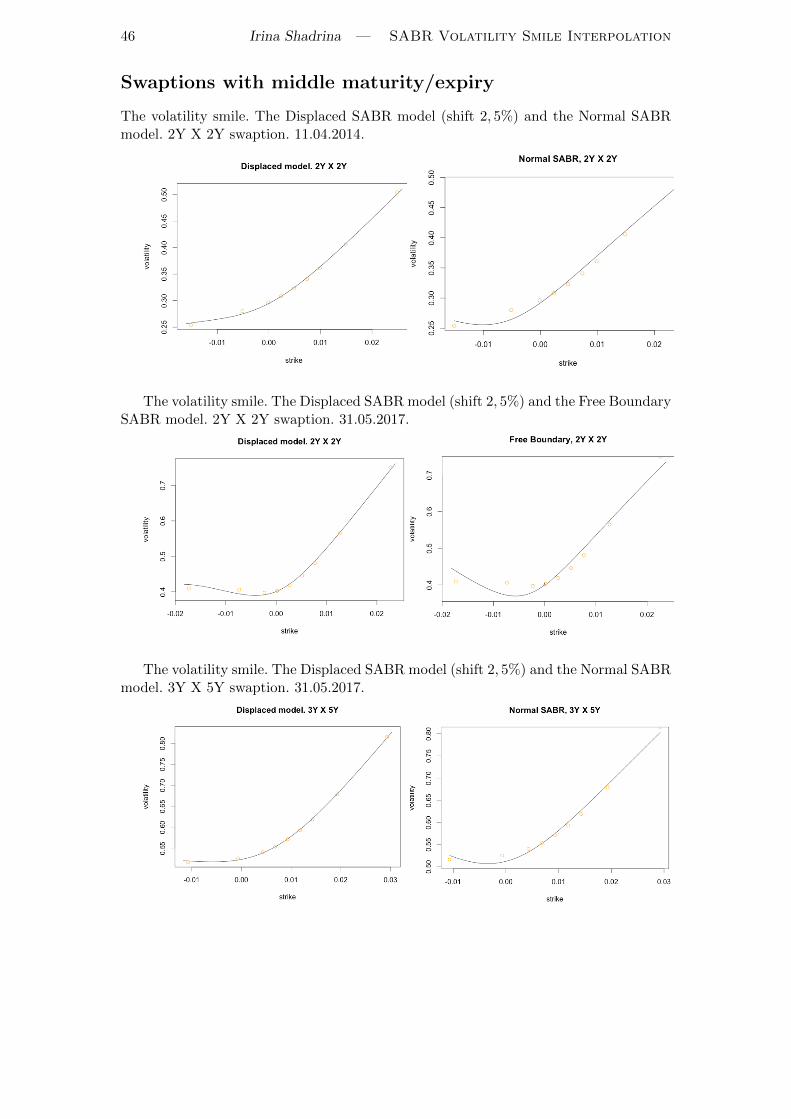
46 Irina Shadrina — SABR Volatility Smile Interpolation
Swaptions with middle maturity/expiry
The volatility smile. The Displaced SABR model (shift 2, 5%) and the Normal SABRmodel. 2Y X 2Y swaption. 11.04.2014.
The volatility smile. The Displaced SABR model (shift 2, 5%) and the Free BoundarySABR model. 2Y X 2Y swaption. 31.05.2017.
The volatility smile. The Displaced SABR model (shift 2, 5%) and the Normal SABRmodel. 3Y X 5Y swaption. 31.05.2017.
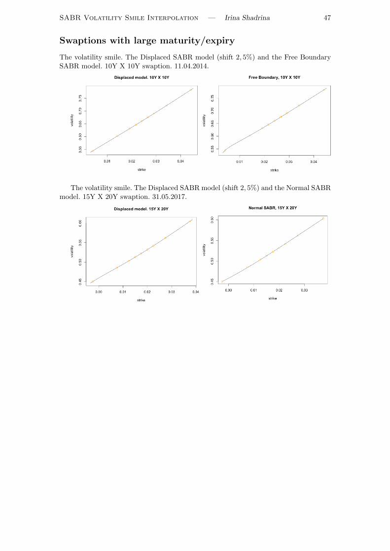
SABR Volatility Smile Interpolation — Irina Shadrina 47
Swaptions with large maturity/expiry
The volatility smile. The Displaced SABR model (shift 2, 5%) and the Free BoundarySABR model. 10Y X 10Y swaption. 11.04.2014.
The volatility smile. The Displaced SABR model (shift 2, 5%) and the Normal SABRmodel. 15Y X 20Y swaption. 31.05.2017.
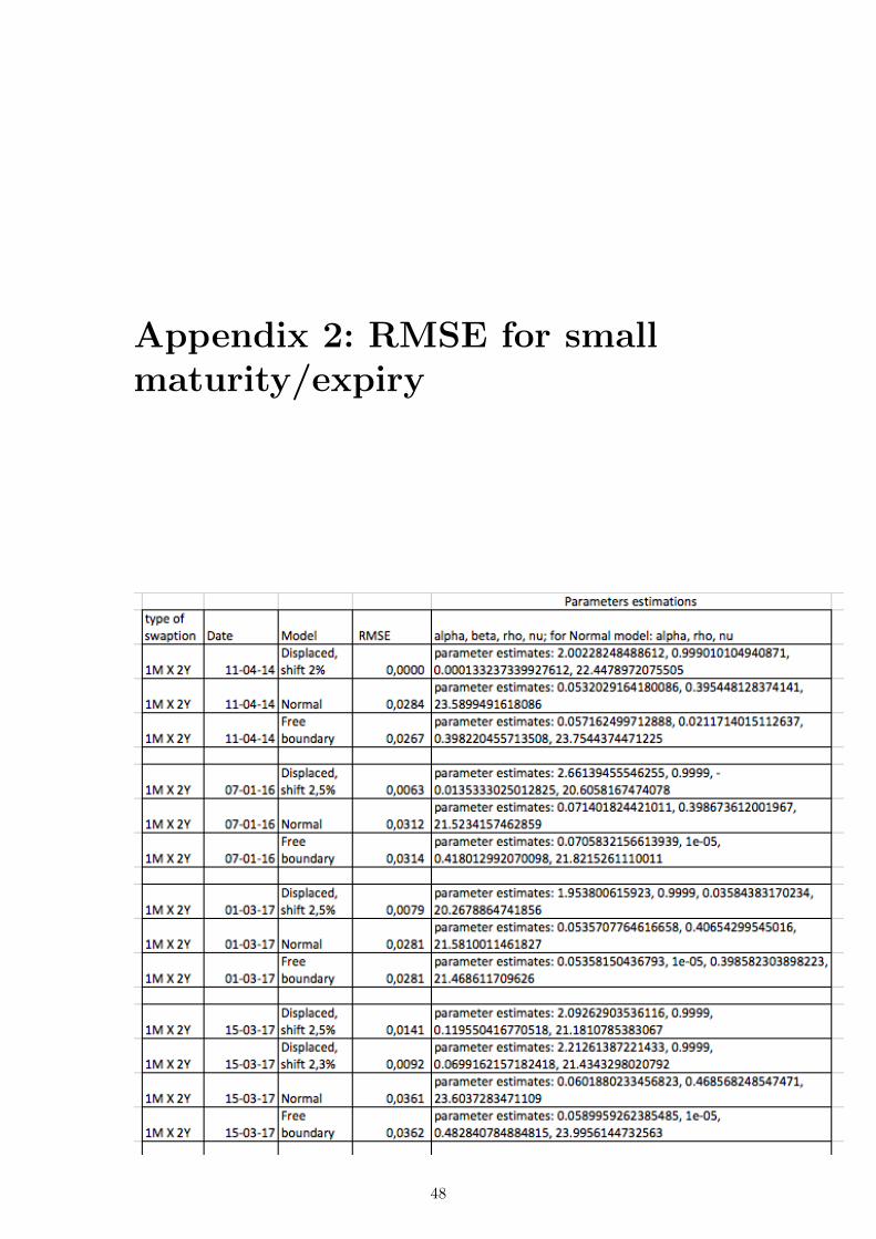
Appendix 2: RMSE for smallmaturity/expiry
48
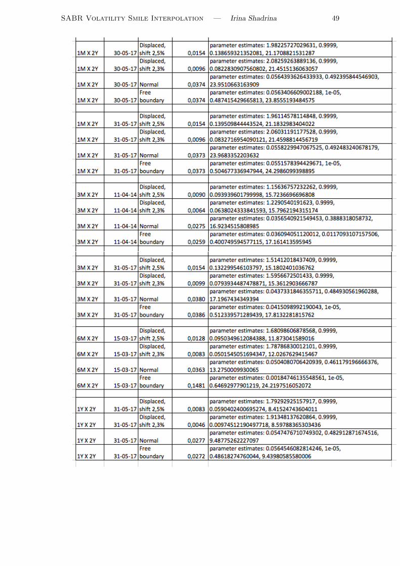
SABR Volatility Smile Interpolation — Irina Shadrina 49
Bibliography
A. Antonov and M. Spector. Advanced analytics for the SABR model. SSRN ElectronicJournal, 2012. URL http://dx.doi.org/10.2139/ssrn.2026350.
A. Antonov, M. Konikov, and M. Spector. SABR spreads its wings. Risk, 26(8):58, 2013. URL http://janroman.dhis.org/finance/SABR/SABR%20spread%20its%
20wings.pdf.
A. Antonov, M. Konikov, and M. Spector. The free boundary SABR: natural extensionto negative rates. SSRN Electronic Journal, 2015a. URL http://dx.doi.org/10.
2139/ssrn.2647344.
A. Antonov, M. Konikov, and M. Spector. Mixing SABR models for negative rates.SSRN Electronic Journal, 2015b. URL http://dx.doi.org/10.2139/ssrn.2653682.
BIS Monetary and Economic Department. Statistical release OTC derivatives statisticsat end-december 2016, 2017. URL http://www.bis.org/statistics/d5_1.pdf.
D. T. Breeden and R. H. Litzenberger. Prices of state-contingent claims implicit inoption prices. Journal of business, pages 621–651, 1978. URL http://dx.doi.org/
10.1086/296025.
A. Etheridge. A course in financial calculus. Cambridge University Press, 2002.
L. Floc’h and G. J. Kennedy. Explicit SABR calibration through simple expansions.SSRN Electronic Journal, 2014. URL http://dx.doi.org/10.2139/ssrn.2467231.
C. Gardiner. Handbook of Stochastic Methods for Physics, Chemistry, and the NaturalSciences. Springer, 2004.
P. Gauthier and P.-Y. H. Rivaille. Fitting the smile, smart parameters for SABR andHeston. SSRN Electronic Journal, 2009. URL http://dx.doi.org/10.2139/ssrn.
1496982.
P. Hagan, A. Lesniewski, and D. Woodward. Probability Distribution in the SABRModel of Stochastic Volatility, pages 1–35. Springer International Publishing, Cham,2015, first draft in 2001. ISBN 978-3-319-11605-1. doi: 10.1007/978-3-319-11605-1 1.URL https://doi.org/10.1007/978-3-319-11605-1_1.
P. S. Hagan, D. Kumar, A. S. Lesniewski, and D. E. Woodward. Managing smilerisk. The Best of Wilmott, 1:249–296, 2002. URL https://www.researchgate.net/
publication/235622441_Managing_Smile_Risk.
P. S. Hagan, D. Kumar, A. Lesniewski, and D. Woodward. Arbitrage-free SABR.Wilmott, 2014(69):60–75, 2014. ISSN 1541-8286. doi: 10.1002/wilm.10290. URLhttp://dx.doi.org/10.1002/wilm.10290.
P. S. Hagan, D. Kumar, A. S. Lesniewski, and D. E. Woodward. Universalsmiles. Wilmott, 2016(84):40–55, 2016. URL https://www.researchgate.net/
publication/295010218_universal_smiles.
50
SABR Volatility Smile Interpolation — Irina Shadrina 51
M. Haugh. Martingale pricing theory. University Lecture, 2005. URL http://www.
columbia.edu/~mh2078/stochastic_calculus.pdf.
M. Haugh. Introduction to stochastic calculus. University Lecture, 2010. URL http:
//www.columbia.edu/~mh2078/stochastic_calculus.pdf.
D. Hohmann, M. Horig, D. Aktuar, and F. Ketterer. The new normal. Technicalreport, Milliman Research Report, 2015. URL http://careers.milliman.com/
uploadedFiles/insight/2015/2079LDP_20150911.pdf.
J. C. Hull. Options, Futures, And Other Derivatives. Pearson Education Limited, 2011.
J. C. Hull and A. White. LIBOR vs. OIS: The derivatives discounting dilemma. 2013.URL http://dx.doi.org/10.2139/ssrn.2211800.
J. Kienitz. Approximate and PDE solution to the boundary free SABR model-applications to pricing and calibration. 2015. URL http://dx.doi.org/10.2139/
ssrn.2647344.
V. Piterbarg. Mixture of models: A simple recipe for a... hangover? 2003. URL http:
//dx.doi.org/10.2139/ssrn.393060.
P. Veronesi. Fixed income securities: Valuation, risk, and risk management. John Wiley& Sons, 2010.
D. K. Youmbi. Implementation of the free boundary SABR model. 2017. URL https:
//ssrn.com/abstract=2996763.