A C O M P A R A T I V E S T U D Y O F M O D E L S F O R P R E D A T I O N

A N D P A R A S I T I S M

by

T. ROYAMA

Canadian Forestry Service, P. O. Box 4000,

Fredericton, New Brunswick, Canada

T A B L E O F C O N T E N T S

Page 1. Introduction 1

2. A brief inquiry into the role of

models in scientific inference 2

3. A background theory of the

structure of predation and parasitism 9

4. The existing models 20

a) The LOTKA-VOLTERRA model 21

b) The NICHOLSON-BAILEY model 24

c) HOLLiNG'S disc equation 31

d) The IVLEV-GAusE equation 35

e) ROYAMA'S model of random

searching and probability of

random encounters 42

f) WATT'S equation 55

g) The T~o~esoN-SwoY equations

for parasitism 61

h) The HASSELL-VARLSY model of

social interference in parasites 66

i) A geometric model for social

interaction among parasites

(this study) 70

Appendix to w 4i. Is the concept

of 'area of discovery' useful in

studies of predation and

parasitism ? 74

j) HOLLING'S hunger model 76

5. Discussion and conclusions 78

6. Summary 84

7. Acknowledgements 85

8. References 85

Appendix 1. The proof of L I = I / 2 R X 88

Appendix 2. The proof of

L z - ~ ( I / 2 ~ - , X R ) / U X - Re- ~rR~'X 88 I _ e - ~ R ~ X

Appendix 3. The proof of eq. (4i. 6) 89

Appendix 4. List of symbols 90

1. INTRODUCTION

ELTON (1935), in his r ev iew of the works of the g rea t b iomathemat ic ian , the late

ALFRED J. LOTKA, wro te :

" W h e n LOTKA publ ished his f irst notes on this subjec t in 1920, an imal ecology

had en te red on a new phase, though we are p robab ly only now beginning to see the

impor tance of it." However , " l ike mos t mathemat ic ians , he t akes the hopeful b iologis t

to the edge of a pond, points out tha t a good swim will help his work, and then

pushes h im in and leaves h im to drown."

When NICHOLSON and BAILEY (1935) publ ished the i r theore t ica l paper, SMITH

(1939) p red ic ted that "in tha t admi rab l e work by NICHOLSON and BAILEY, 'The

Balance of An ima l Populat ions ' , wil l be found enough populat ion p rob lems to keep

s e v e r a l l abora tor ies busy for the nex t twen ty years ."

Shor t ly a f te r the publ icat ion of these theore t ica l works, there arose among ecolo-

gists a storm of controversy which has lasted for more than 20 years ~nd hss not

yet subsided. Much of the dispute has been based on varying degrees of mutual

misunderstanding, and many innocent students of natural history have perhaps been

drowned. Nevertheless, theoretical approaches and mathematical concepts still play

an important role in animal population ecology, chiefly for the following reason. In

the study of population processes, what we can observe is an integrated complex of

factors. But the elemental components and their interactions are not always apparent

and indeed may even be impossible to detect by ordinary observation. Wherever

unobservables are involved, they must be detected through reasoning by analogy.

For the past decade, biomathematics and statistics have become increasingly more

sophisticated, while the students of natural history have by observation accumulated

a vast amount of information on animal behaviour. Yet, there seems to be an increas-

ing gap between the two approaches. My aim is to bridge this gap, and the scope

of this paper is to show what the existing theories on predation and parasitism really

mean, and what role these theories would, or would not, play in leading to an under-

standing of predation processes in relation to population dynamics.

Before the existing theories are critically reviewed, I shall discuss the role of

models in general terms and then consider some basic attributes of predation and

parasitism. In fact, these two sections are the result of my comparative study of the

existing models rather than a starting point. Nevertheless, this part of the conclusion

is presented first because the argument can then be more readily followed.

2. A BRIEF INQUIRY INTO THE ROLE OF MODELS IN SCIENTIFIC INFERENCE

To make a critical study of existing predation (parasitism) models, we need to

have a clear idea of what a 'model' is. However, the concept of models in science

varies from one case to another, depending on what is aimed at in each individual

case. Thus it is perhaps better to examine the past use of the word rather than to

begin with an attempt to define it.

The word 'model' has been used more or less synonymously with: an assumption;

a hypothesis; a proposition; a theory; a law; or even a mere mathematical equation.

A typical example and positive justification for this broad usage of the word is found

in WALKER (1963, p. 4) :

"The word model in a particular sentence may refer to one or more of many

related aspects of the general notion. Thus cortical model refers to the model as it

is recorded in the structure and arrangement of molecules in the memory banks of

the brain. Conceptual model refers to the mental picture of the model that is intro-

spectively present when one thinks about the model. This picture probably corresponds

to some scanning process over the appropriate memory banks. The verbal model

consists of the spoken or written description of the model. The postulational model is a certain type of verbal model that consists of a list of the postulates of the model.

The geometrical model refers to the diagrams or drawings that are used to describe

the model. The mathematical model refers to the equations or other relationships

that provide the quantitative predictions of the model. The material model is the

arrangement and interactions of fundamental particles, their fields and aggregates.

When a writer refers to the 'Bohr model of the hydrogen atom', he may have in

mind any or all of these aspects; the reader must select the aspects appropriate to

the context."

WALKER'S broad usage of the word includes, in later chapters of his book, the

MENDELIAN law of inheritance and the DARWINIAN theory of natural selection as

models. Clearly, the word 'model' in WALKER'S sense is used to categorize similar,

but distinctly different notions in a single, convenient, descriptive term. This catego.

rization may at times be needed in scientific communication, but I would rather use

the word in a much restricted sense in this paper, in order to emphasize the role of

a certain type of model that distinguishes itself from other similar notions, e.g.

'assumptions', 'hypotheses', 'theories', or 'descriptions' of laws and rules.

A dictionary (e. g. The WEBSTER's Third International Dictionary, 1968) treats

the word as a synonym for : Example, Pattern, Exemplar, Paradigm, Ideal, etc.; or it

is something perfect of its kind. The dictionary also states that a model is: a thing

that serves as a pattern or source of inspiration for an artist or writer; or an analogy

used to help visualize, often in a simplified way, something that cannot be observed

directly. The last definition is particularly important and most relevant to my inves-

tigation.

WALKER further stated that "the main purpose of a model is to make predictions",

and that "if a mathematical model predicts future events accurately, there is no ne-

cessity for any interpretation or visualization of the process described by the equation."

These statements should be interpreted with caution, however. If they are taken

literally, it might be concluded that the purpose of an assumption, hypothesis, theory,

etc. is to predict but not to aid understanding of natural order: that is to say,

WALKER'S statement might be taken erroneously as synonymous with 'the aim of

science is predictions'. TOULMIN (1961) pointed out that the ancient Babylonian

astronomers who predicted the motion of stars amazingly accurately by arithmetic

means failed to understand underlying mechanisms, while the Ionian philosophers'

crude model of the universe eventually led to 20 th-century physics.

The understanding of natural order is achieved through the formation of new

concepts. SCHON (1967) emphasized the role of metaphor in the formation of a new

concept, through which a novel idea or discovery was made. He maintained that the

new concept would emerge by shifting already existing concepts to a new situation

by metaphor. That is to say, the old concepts, shifted to the new situation by meta-

phor, are models for the new concept. If we use the word 'model' in a similar way,

and I am inclined to do so here, then some of WALKER'S examples should be exclud-

ed.

For example, the DARWINIAN theory can be a model if its principle is shifted

and applied, say, to social phenomena, but as long as the theory remains in the domain

of organic evolution I do not call it a model. Similarly, while the MENDELIAN law

itself is by the same token not a model of M~NDELIAN inheritance, its principle can

be demonstrated by a model in which equal numbers of red and white balls in a jar

are sampled at random, two balls at a time. The statistical expectation of the propor-

tion of white-white pairs is one-quarter of the total number of pairs drawn. This

model can be stated by a simple mathematical equation, and the equation is just the

means of statement. The equation as a statement of the model can at the same time

be a statement of the law, since the symbolic expression for both the model and the

law takes the same form. By means of the balls-in-a-jar model, however, the empirical

law found by MENDEL becomes understandable and intelligible, and the model leads

to the postulation of particulate inheritance--a hypothesis; the reliability of this hypo-

thesis is tested in an organized way against further observations until it emerges as

a biological theory and principle.

We should distinguish, however, between an equation as a general, symbolic

method of statement, and one as a mathematical operation as a means of reasoning. In

a model as simple as the balls-in-a-jar example, the mathematical probability of a pair

of one kind, say white-white, may be obtained intuitively and correctly (i. e. a priori),

whereas often a more complicated mathematical operation is required to draw a con-

clusion. An equation that states a result of inferences should therefore be distinguished

from an equation which is adopted as a convenient description of an empirical law,

such as a polynomial equation obtained in curve-fitting by the least squares method.

The latter is generally not the statement of a model nor a hypothes is ; i t is merely

one casual and tentative way, among many others, of describing what has been

observed, although it may at times play a certain role in the formulation of ideas,

as a tentative part of a model.

In a very few cases, an empirical law can be stated accurately by a simple math-

ematical equation in which the value of every coefficient involved is clearly defined,

but without understanding. A typical example of this is NEWTON'S gravitational law,

i.e. the force of gravitational interaction is proportional to the product of the masses

of two interacting bodies and inversely proportional to the square of the distance

between them. This is an accurate statement. It should be noticed, however, that

even this accurate statement of the universal law had no rational explanatory model

behind it until the early 20 th century when EINSTEIN explained it in his relativistic

theory of gravity (GAMoW 1962).

A similar example is seen in the logistic law in demography first formulated by

VERHURST (1838), which was later generalized to population growth in other animal

species by PEARL (1927). The VERHURST-PEARL logistic law assumes that the instan-

taneous rate of increase per animal is proportional to the still unutilized opportunity

for growth, and is expressed in the well-known mathematical equation. But no positive

rationalization of the assumption has been m a d e ; t h e r e is no rational relationship

between the assumption (CHAPMAN's (1931) concept of 'environmental resistance')

and the attributes of the subject (population growth), so the latter remain unknown.

The logistic equation was derived through metaphoric inferences rather than through

comparisons between the attributes of the subject and those of a model in which

factors involved are known.

Thus, we can see that differences between (a) a deductive model (deduced only

by reasoning) and (b) a descriptive equation like that of the logistic law, lie in

differences between (a) a comparison of components in the subject with equivalent

parts of the model and (b) a metaphoric juxtaposition of the observed trend of the

subject with that of some known concepts.

While the importance of metaphor, as SCHON (1967) emphasized, is appreciated,

it should be borne in mind that metaphor alone does not necessarily lead to explana-

tions and understandings. Quoting one of SCHON'S examples, the original concept of

'foot', restricted to an animal's foot, can be shifted to a much broader concept includ-

ing 'the foot of a mountain'. Although this example certainly shows the importance

of metaphor in, say, the evolution of languages, such juxtaposition does not immediately

imply the understanding of the structure of the foot of mountains. In other words,

metaphor, playing its important role in one situation, or in a certain part of the proc-

ess in the formation of ideas, can be too vague to be useful in another. In the

example of the logistic law, metaphor led to the formulation of the equation that can

often describe observed relationships satisfactorily, but such success often depends

on how the observed relationships are described deterministically.

Normally, in the field of population ecology, a deterministic description of phenom-

ena is often so difficult that a descriptive, empirical equation can be adopted only

casually. Such casual equations often involve some coefficients whose nature is not

known. The equation is then hard to rationalize as there can be some other forms

of equations which fit the same observation equally well. Also, the coefficients must

be estimated from a limited set of observed data (our observations are, at any rate,

limited), and the more limited the number of observations, the less generalized the

estimate will be. Further, the more coefficients that are involved and that need to be

estimated, the more flexible the equation becomes since the degrees of freedom for

fitting increase. The above statement simply suggests that a good fit does not imply

that the equation concerned explains the mechanism.

Conversely, if an equation, derived from metaphoric inference, did not fit observed

relationships, it would have to be rejected. The rejection, however, involves a risk

of rejecting a correct assemblage of right components. This is because the disagree-

ment could be due to some other components or conditions which were missed, and

not due to inappropriate metaphor; if this is so, the equation need not be rejected

but only improved by further search for these overlooked factors. The difficulty is,

however, that there is no systematic way to know whether the disagreement is due

to the inadequate assemblage of factors or to inappropriate metaphor.

Hence, the fitting of an empirical equation to observed relationships in certain

subjects, and I imply that animal predation is one such subject, has a limited value

theoretically. In the following, another method, i.e. analogies by attributes, will be

explored.

Normally, reasoning starts from a set of tentative propositions. This set of

propositions is one kind of hypothesis. Because it is only tentatively assumed, it does

not necessarilly and immediately postulate mechanisms underlying the subject.

Often, an early, tentative hypothesis is a mere collection of all the factors that

can be conceived, whereas what one can observe is the integrated complex of factors

interacting with each other. It is, however, difficult in many cases to extract each

component of the subject to compare with an assumed one purely by the observational

method. It is possible, instead, to integrate the assumed components on a theoretical

basis so that the assumption-system can be compared with the observed whole. The

difficulty is that a mere list of components will not necessarily provide the method

of integration. By some means, we have to assume the structure as well. It is at

this stage that analogies can play a role, and it is the structure thus derived from

analogies (or some known examples) that I call a 'model' here. When the model to

adopt is determined, a method of calculating the model's attributes will follow. An

analytic (i. e. mathematical) method can be used for the calculation, or the method

commonly called 'Monte Carlo simulation' may be useful. Here, mathematics is used

not as a convenient means of description, but as a means of inference.

Now, we recognize two early stages of inferences; the collection of components,

and the arrangement and integration of them by a tentative model. The tentative

model may be called a hypothesis, but it should be borne in mind that it is only

tentative and not more than a convenient assumption. Such tentative hypotheses do

not enable us to postulate the mechanism of the subject. The tentative hypothesis,

however, is now compared with observation and will in general need refinement, as

it often does not agree with the facts with a desirable degree of precision. A refine-

ment will be made through alteration of the arrangement, adding some more compo-

nents which have previously been missed, etc. As the stage of refinement advances,

the hypothesis would enable one to postulate more confidently. Finally, as the degree

of agreement with the facts increases, the postulational hypothesis would eventually

emerge as a theory or even a principle.

There are three important points in the gradual process of inferences mentioned

above; they will be discussed more in detail below. First is the formulation of a

tentative hypothesis; second, the evaluation of agreement ~nd disagreement between

the theoretical and the observed; third, the fact-observation relationship. The third

one is a question of whether an observation can be accepted as fact.

For the following discussion, some symbols will be used as defined below:

0 : the result of observation,

Ko : t he set of all major components involved (not particularly known) in the

observed system,

So : the structure of the observed system,

KA : the set of all assumed components in the model system,

S~ : the structure of the model system,

E : theoretical expectation deduced from KA and S.x.

When E and 0 are compared, we will get either an agreement or a disagreement,

i.e. E=O or E r respectively, to which various conditions (causes) contribute as

below:

Conditions

C1. K~ and S~ are involved in Ka and So respectively (so that both K~4 and S~

are, at least, not false).

cu. if KA and S~ are both sufficient, then E=O.

c~2. if either KA or S:~ is inadequate, then E ~ O.

c~a. if O is false or inadequate under c~I, then E:~O.

Cz. Ko does not involve the whole of K~, and/or So does not involve the whole

of S.~ (so that KA and/or S.n are/is, at least partly, false),

c21. if false parts of Ka and Sn, or false parts of O and K~, (or S:,z), are

adjusted so that they cancel out each other, then E - O .

c~2. if not c21, then Er

Now, one can claim that his hypothesis is right only when c , under C~ holds.

However, the fact that an agreement (E~O) exists is not sufficient to establish the

hypothesis, since E=O also occurs when c~1 under C2 is involved. Therefore, if a

comparison between E and O is the only available method, we have to be contented

with an assessment of the relative credibility of these causes. The assessment can

be done much the same way as for the calculation of the LAPLACIAN probability (see

BURNSIDE 1928 ; POL~CA 1955).

Let Pr {E=O} be the probability of event (E=O) taking place. As it takes place

either when cu or when C~l is involved (the probability of which will be written as

Pr {(E=O) ]c~} and Pr {(E=O) Icy} respectively), we get

Pr{E=O} =Pr{(E=O) i c~} +Pr{(E=O) !c2~.

Also, as C~l is dependent on C~,

Pr{(E=O) [c,} =Pr~c,}Pr{C~}

and similarly,

Pr { (E= O) I ce~} =Pr {c~x} Pr {C~}.

From these formulae, the following conclusions are drawn. If Ka is comprised

of only those components which are either axiomatic, a priori (known to be true

without appeal to the particular facts of evidence), or can be deduced from concepts

already known to be true, Ka must be involved in Ko. In other words, Pr {C~} is

high but Pr {C2~ is low. Therefore. if an agreement (E=O) was observed under

these circumstances, P r { ( E - O ) [cH[ is high as compared with Pr {(E=O) lc2~} ; i. e.

the credibility of reasoning that the agreement is due to a right hypothesis is com-

paratively high. However, the more axiomatic K~ is, the lower Pr {cn} will be, and

so the less likely is event (E=O) to occur.

For the above reason, a simple, deductive model often fails to agree with obser-

vation. But such failures in deductive models are more likely to be caused either

by c~2 or c~3 than by c2z. If so, there is no reason to reject the hypothesis ; it only

needs further elaboration. The only case in which at least a part of the components

or the structure should be rejected, is C~. Here, a careful observation of the disagree-

ment is of paramount importance.

There are, broadly speaking, two possible kinds of alterations when a disagree-

ment is observed. A method frequently seen in the literature is to adjust the struc-

ture of the model or to add some more components to obtain E=O. Here, Pr{E=O}

certainly increases, but at the same time there is a risk of getting a high Pr{C2}, and hence Prl(E=O)[c21}. The risk is greater if the added components are those

whose trend is not fully understood. The estimation of coefficients involved in the

empirical equation could amount to this kind of adjustment, as the coefficients often

have to be estimated by comparing E with O. The recent predation models in fact

involve such a risk, as will be shown later. The worst thing is to obtain E=O by

adjustment when the first disagreement was in fact caused by c22 ; it only increases

Prl(E=O)]c21} and has no meaning at all.

The second type of improvement is to look for more of the axiomatic components,

or of those which are known to be true for any reason, without making a particular

effort to obtain E=O. This keeps Pr {C2} to a low level, and therefore the improve-

ment, if any, increases, though only gradually, Pr {c1~}.

Although the second method will provide a steady approach to the goal, a question

arises whether a collection of axiomatic assumptions can eventually produce a suffi-

cient model. WALKER (1963) argued that "it is a common misconception that new

models are constructed by strict logical deduction from observed facts and from

previous models". Certainly, nothing new will come from mere accumulations of

known concepts. However, a model is not a mere collection of already known com-

ponents but involves a positive recombination of them which is applied to a new

situation. And the role of the model is to produce a useful recombination by analogy.

The efficiency of finding a useful model depends on the efficiency in selecting

axiomatic components and recombining them. A model is therefore required to have

room for accommodating added components and recombining them. This calls for

a general and idealized model to start with: too specific a model has to be rejected

upon finding a disagreement because of its limited capacity for modification, or it

could involve a high value of Pr{(E=O)Ic2~}, particularly when some coefficients

involved have to be estimated rather than determined by independent and direct

observations of what these coefficients' represent.

The role of idealization is again seen in the history of the physical sciences,

which should be understood in the context of fact-observation relationships and of

the notions 'realistic' and 'unrealistic'. In the ARISTOTELIAN doctrine, certain natural

phenomena as observed were taken for granted as axioms. Thus, a cart pulled by a horse

(a constant force) moves at a constant speed, but comes to a stop (a natural state

of rest) when the force is removed. Inorganic chemical processes were explained by

analogy with physiological processes, such as seeds becoming ripe, which were accept-

ed as natural, axiomatic, and were not questioned.

A significant change in the way that natural order was regarded came at the

t ime of the Renaissance when BURIDAN (OPPENHEIMER 1956), and later GALILEI,

made the earliest announcement of the principle of physical inertia. In 1612, GALILEI

wrote to a pupil of his:

"For I seem to have observed that physical bodies have physical inclination to

some motion ...... through an intrinsic property ...... And therefore, all external impedi-

ments removed, . ..... it will maintain itself in that state in which it has once been

placed" (translation by DRAKE 1957).

The recognition of the "physical inclination through an intrinsic property" is

important, in the context of the present discussion, as GALILEI could not have been

able to observe a ship floating on a perfectly calm, smooth, resistanceless water and,

once pushed, moving at a constant speed without the faintest sign of slowing down.

The discovery, or recognition, of inertia must therefore have been made with only

an idealized situation in mind, a situation which to other natural philosophers of the

period must have been 'unrealistic'. A similar example is found in the history of

chemistry, when the existence of chemically pure substances was recognized only

under idealized, artificial, and therefore unnatural conditions (TouLMIN 1961).

These examples illustrate the point that a fact as observed in a natural state is

not ultimate, for it is only the visible part of the whole. Inferences by models can

only help one to generalize an observation, and, as POINCAR~ (1952) pointed out,

"without generalization, prediction is impossible". It is perhaps particularly true with

ecological studies that generalization is possible, not in a thing in itself which we

observe under natural conditions, but in an idealized situation. Here, analogies by

models play an important role.

3. A BACKGROUND THEORY OF THE STRUCTURE OF PREDATION AND PARASITISM

In the first place, it will be made clear that what I mean by 'background' in this

section involves only those components and conditions which, under each idealized

assumption, are known a priori; that is, they are known to be involved in the ideal-

ized process of predation and parasitism without any need of confirmation by observ-

ation. The need for such theories is undeniable since, as already pointed out in w 2,

they are the starting point for gradual inferences. It should be borne in mind that a

direct comparison of this background theory with any observation might result in

disagreement; but such disagreement, unlike that caused by condition c~2, will not

invalidate the theory.

10

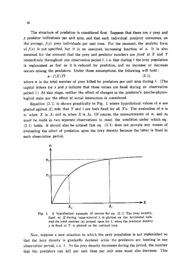
The s t ruc tu re of preda t ion is cons idered first. Suppose tha t there a re x p rey and

y p reda to r individuals per uni t area, and tha t each indiv idual p reda to r consumes, on

the average, f(x) prey individuals pe r uni t t ime. F o r the moment , the analyt ic fo rm

of f(x) is not specified, but it is an assumed, increas ing function of x. I t is also

assumed for the m o m e n t that the p rey and p reda to r numbe r s are fixed at X and Y

respec t ive ly th roughou t one observa t ion per iod t, i .e . that dur ing t the p rey populat ion

is rep lenished as fast as it is r educed by predat ion, and no increase or decrease

occurs among the preda tors . Under these assumpt ions , the fo l lowing will hold :

n-~f(X) Yt (3.1)

where n is the total n u m b e r of p rey ki l led by p reda to r s pe r uni t area du r ing t. (The

capital l e t t e r s for x and y indicate tha t these values are fixed dur ing an observa t ion

per iod t.) A t this stage, ne i ther the effect of changes in the p reda to r ' s psycho-phys io-

logical s ta te nor the effect of social in terac t ion is considered.

Equat ion (3.1) is shown graphica l ly in Fig. 1 where hypothet ica l values of n a re

plot ted agains t X; note that Y and t a re both fixed for all X's . The evaluat ion of n is

nl when X is X~ and n2 when X is Xz. Of course, the me a su re me n t s of n~ and n~

mus t be made in two separa te observa t ions to mee t the condi t ion under which eq.

(3.1) holds. I t should also be not iced tha t eq. (3.1) does not provide any means of

eva lua t ing the effect of preda t ion upon the p rey dens i ty because the la t te r is fixed in

each observa t ion period.

rl

n~

N y X2

>• Xl

Fig. 1. A hypothetical example of curves for eq. (3. 1) The prey density, fixed at X during time-interval t, is plotted on the horizontal axis, and the total number (n) preyed upon for t, when the predator density y is fixed at Y, is plotted on the vertical axis.

Now, suppose a new si tuat ion in which the p rey populat ion is not rep lenished so

tha t the p rey dens i ty is g radua l ly deple ted while the p reda to r s a re hunt ing in one

observa t ion period, i . e . t . As the p rey dens i ty decreases dur ing the period, the n u m b e r

tha t the p reda to r s can kil l per uni t t ime per uni t area m u s t also decrease. Th is

11

situation is easily seen from Fig. 1. Suppose XI, is the initial prey density. At this

moment, the prey are killed at the rate of n J Y t . But if the prey density is depleted

to X2, the rate of predation is decreased to n~/Yt. Hence, the overall rate of predation

must be something between n l / Y t and n2/Yt. To evaluate the overall rate of predation,

we must use calculus.

As mentioned before, eq. (3.1) holds only when the prey density does not change

during t. In our new situation in which the density x decreases as t increases, eq.

(3. 1) holds only for such a short period that a reduction in x at this moment can

practically be ignored. Let us denote this short period by `it and an accordingly small

fraction of number killed by `in. Substituting x, `it, and `in for X, t, and n respectively

in eq. (3.1), we have

`in = f ( x ) Yztt, or ` in/dt =f(x) Y (3.2)

and for `it->0, we have

d n / d t : f ( x ) Y (3.3).

Clearly, the derivative d n / d t is the rate of capturing prey, and so it is a positive

function of x. If, however, the rate of depletion in prey density, i.e. dx /d t , is consi-

dered, it is a negative function of x, but its absolute value must be equal to dn /d t ,

because the prey population is reduced according to the number consumed. So, we

have

d x / d t = - f ( x ) Y (3.4).

Let xo be the initial prey density (when t=0) which is reduced to x over a period

of time, i.e. t, and integrating eq. (3.4), we have

f x (3.5). dx

= - xo f C x i -

Now, I shall explain in more detail the reason why the differential equation and

the integration (i. e. eqs. (3.4) and (3.5) respectively) are used as a means of deduction,

because this means of deduction should be understood thoroughly so that my criticism

of various models in later sections will be followed readily.

Suppose that the initial prey density was xo when t=0, and that it took `ito to

reduce the prey density by ,Ix. Assuming that `ito and so `ix were sufficiently small,

and substituting xo, - ` ix , and `it0 for x, `in, and `it in eq. (3.2), we have

Ydto = - ` i x / f (xo) .

At this moment, the prey density is reduced to Xo-`ix. Suppose, for further reduc-

tion in the prey density by as much as `ix, it took `itl. Then for the same reason as

above, we get

Y`it~ = - ` i x / f ( xo - dX) .

In general, at the i th interval, it takes `its to reduce the density by another `ix. As

the prey density has been reduced to xo- i ` i x by this time, the evaluation of `it~ is

given by

12

Y Jr, = - J x / f ( x o - i J x ) .

Thus we have the following summation :

YJto = - J x / f ( x o )

Y J t , J x / f ( x o - ,fx)

Y~at~ = - J x / f (xo - 2Jx)

+) Y J t , = - J x / f ( x o - i J x )

i i Y Z J t , = - ~ { J x / f ( x o - iJx) }.

i = 0 i = 0

Now, let t be the total time taken to the i th interval. Then t is the summation of

all J t 's to the i th interval, i.e. i

t = ~ d t , i = 0

so that i

Y ~ , f t , = Yt . i - O

Similarly, let x be the prey density at the i th interval, which is the difference between

the initial density xo and the total number of prey taken per unit area, i.e. iJx . So,

X = X o - i J x .

As x is a continuous variable, we can make Jx infinitesimally small, which is now

written as dx. Also, under these circumstances, the summation sign ~ is replaced by

the integral sign ~. Further, it is clear that x varies from xo to x when i varies from

0 to i. Thus

i f x dx l im ~ { J x / f ( x o - lax) } : f ( x ) "

Jx~O i~O xo

Hence, y t = _ f ; ~ d x f(X)' and we have eq. (3.5).

For further discussion, the integral in the right-hand side of eq. (3.5) must be

evaluated. As the form of f ( x ) has not been specified, a few forms will be assumed

below for convenience.

Let us assume first that f ( x ) is a linear function of x ; that is, the prey are killed

in proportion to their density. Then,

f ( x ) = a x (3.6)

where a is any positive constant. As will b e seen later, eq. (3.6) is the basis of the

classical models by LOTKA (!925), VOLTERRA (1926), and NICHOLSON and BAILEY

(1935), but I shall not discuss its ecological meaning as this is not needed at the

moment. Substituting the right-hand side of eq. (3.6) for f ( x ) in eq. (3.5), we have

a Y t = - ( x d x d xo X

which yields

a Y t = - In x (3. 7). Xo

13

As the prey density is reduced from Xo to x during time t, the difference (xo-x) is

the number of prey individuals killed per unit area during t. So, removing the 'ln'

sign and rearranging, eq. (3. ,7) will be solved with respect to x o - x as below,

Xo - x = Xo ( 1 - e - ~ ' )

or, setting z equal to Xo--X,

z =Xo (1 - e -art) (3.8).

This is in fact the familiar NICHOLSON-BAILEY 'Competition equation' (see w

Now we have three variables in eq. (3.8), z being the dependent variable and

x0 and Yt independent ones. In this particular example, the predator density Y and

the t ime t (for which the prey population is exposed to predation) are mutually com-

plementary. That is to say, the effect of predation upon prey density exerted by twice

as many predators for half the time, is exactly the same as the effect by half as many

predators for twice the t ime since

(2 Y) (t/2) = (Y/2) (2 t).

This holds only because neither social interference (or social facilitation) among pred-

ators nor changes in physiological state are considered: they have been ignored,

for the t ime being, for simplicity.

Under the above circumstances, eq. (3. 8) represents a surface in a three-dimen-

sional coordinate system, i.e. the z-, x0-, and Yt-axes, in which z is the only

dependent variable, and x0 and Yt are mutually independent. This does not mean

that Yt is ecologically independent of x0, particularly in a closed system in which the

predator density in one generation is determined by the prey density in the preceding

generation. But, within a generation, Yt and xo are mathematically independent of

each other, in the sense that we can think of any Yt-value for a given x0-value.

Figure 2a shows a surface generated by eq. (3.8), the surface being determined

primarily for a given value of the constant a.

In this figure, any cross-section of the surface parallel to the Z-Xo plane is linear,

which suggests that for any fixed value of YL the number of prey killed per unit

area increases linearly with the initial prey density. However, the cross-section parallel

to the z -Y t plane is exponential, suggesting that for any fixed value of x0, the share

of food for each predator decreases progressively as the predator density increases,

or it becomes progressively harder for each individual to find its food as the t ime

spent hunting increases. This is in fact the 'law of diminishing returns' when the

predators put more effort (or predator-hours, i.e. Yt) into hunting.

If both sides of eq. (3. 8) are divided by x0, then

Z/Xo: (1-e -~') (3. 9).

The right-hand side of eq. (3. 9) does not involve x0, and therefore z/xo is uninflu-

enced by changes in x0. Graphically, the surface on the Z/Xo-Xo Yt coordinate system

is perfectly parallel to the xo-Yt plane so that the cross-sections parallel to the z/xo

-Y t plane maintain a constant shape along the x0-axis (Fig. 2b) . Under these

circumstances, we do not need a three-dimensional coordinate system but a simple

14

Z-Xo PLANE ~ . . . ' ~

0 Xll ~

Fig. 2a. An example of surfaces generated by eq. (3.8). x0 is the initial prey density, Yt the hunting effort (i.e. predator-hours), and z the reduction of the prey density at the end of the interval t.

A zl~-x, PLANE

,*'"'i

Fig. 2b. Same as Fig. 2a, but the proportion of the prey density reduced from the initial density, i.e. Z/Xo, is plotted on the vertical axis, cf. eq. (3. 9).

two-dimensional one, i .e. a Z/Xo-Yt system. This is in fact the method of presenta-

t ion originally used by N[CHOLSON (1933) who called the curve the 'competi t ion curve' .

This simple method of presentat ion is possible, however, only under the part icular

15

assumption that f(x) is a linear function of x. If f(x) is not a linear function, gener-

ally speaking, the x0-axis is still required since the ratio z/xo again changes as x0

changes, This will be shown in the following example.

Observations by various authors have shown that the function f(x) is not normally

linear, and there is a good reason to believe that it should not be so (see w 4c). In

fact, f(x) is more like the curve shown in Fig. 1, which increases as x increases but

gradually approaches a plateau. This type of curve can be generated by various

equations. For convenience, however, we shall assume the following function used

extensively in IVLEV'S (1955) s tudy on fish predation (see w 4d):

f(x) -~ b (1 - e- a,~) (3.10)

where b and a are any positive constants. Al though the biological meaning of this

equation is as open to cri t icism as the NICHOLSON-BAILEu one, this is not important

at the present stage of the argument .

Substi tuting the r ight-hand side of eq. (3. 10) for f(x) in eq. (3.5), we have

Y t = - f x dx (3.11), xo 1 -- e - ~

which yields

1 ln{(l_e_axo)e_~br~+e_~,, } (3.12) Z - - a

where z = x 0 - x.

Equation (3. 12) generates a surface on the z-xo-Yt coordinate sys tem (Fig. 3a)

which has a more complex shape than that generated by eq. (3.8) or Fig. 2a.

Al though the cross-sections parallel to the z-Yt plane are very similar to those in

Fig. 2a, as they also represent the law of diminishing returns, those parallel to z-xo

Fig 3a.

Z

�9 -,.. \ " , , :~ �9 ., \ -,. :

0 x ~

Same as Fig. 2a, but the surface is generated by eq. (3. 12).

16

Fig. 3b.

z/x, T x o PLANE

/ / / ,' !"--r , j,

0 • ~

Same as Fig. aa, but proportion z/xo is plotted on the vertical axis.

plane are also curvilinear and similar to the curve generated by eq. (3. 10), Clearly,

we cannot present eq. (3. 12) in a two-dimensional coordinate system showing the

relationship between Z/Xo and Yt, since the relationship changes as Xo changes (Fig.

3b).

These two examples show that, though no ecological reality is attached to them

at the moment, the number of prey killed by predators per unit area, i.e. z, is expressed

as a function of two independent variables (x0 and Yt). So we can write this rela-

tionship in a general form using a functional symbol F as

z = F (Xo, Yt) (3.13).

Equation (3. 13) will be called an 'overall hunting equation' iand the function F

an 'overall hunting function' as opposed to eq. (3.1), or (3.4), which is called an

'instantaneous hunting equation' and the function f an 'instantaneous hunting function'.

(The instantaneous hunting function may be a function of x, y, and t as a general

case ; see later. ) The essential difference between the overall and the instantaneous

equations is that the former involves the effect of diminishing returns whereas the

latter holds only at an instant and so does not involve this effect. If one intends to

build a model to study a predator-prey interacting system, what is needed, from a

theoretical point of view, is the overall hunting equation, since this is the equation

which provides the estimates of the number of prey killed and of the final density

of prey at the end of a hunting period. The former estimate gives a basis for calculat-

ing the number of predators' progeny and the latter the number of prey's progeny.

Equation (3. 13), however, does not take into consideration a number of other

factors which are likely to be involved in an actual predation process, e.g. the effect

17

of social interactions among predators and the effect of hunger. One way to incorpo-

rate these factors and~ their influence on the form of an overall hunting equation will

be shown in the following paragraphs.

Social interactions among predators may be classified into two major categories,

social interference and facilitation. These cause a reduction or increase, respectively,

in the instantaneous hunting efficiency of each predator as compared to what it would

potentially exhibit if these factors were not operating (for a detailed discussion, see

w 4i). Let S be the factor by which f ( x ) is reduced or increased. Then an effective

instantaneous hunting function will be Sf(x) . Also the effect of social interaction

must vary as the densities of both predators and prey vary. For instance, too many

predators hunting too few prey would experience more intense interference, than other-

wise, among the predators. Therefore, S must at least be a function of both Y and x,

which will be written as S (Y, x). Incorporating the factor S (Y, x) into eq. (3.4),

we have

dx /d t= - S ( Y , x) f (x) Y (3. 14),

and so

Yt = _ ~,jx dx (3.15). xo S (Y, x) f (x)

However, the intensity of social interaction might change with time, in which case, S

may also be a function of t. The complex function S f in eq. (3.14) is a generalized

instantaneous hunting function and can be written as f (x , Y ) , and for further gener-

alization as above it may be written as f (x , Y, t). But I shall avoid such complica-

tions at the moment.

The integral on the right-hand side of eq. (3.15) generally involves Y but not

t. This suggests that if z ( = x o - x ) is evaluated in eq. (3. 15), it would be a function

of xo, Y, and t, rather than one of x0 and Yr. Here, Y and t no longer form a single

complex variable. Thus the overall hunting equation becomes

z =F(x0, Y, t) (3.16).

Equation (3. 16) has three independent variables, and so it can be presented only

in a four-dimensional coordinate system, or more practically in a series of three-dimen-

sional coordinate sys tems ; i f , for instance, z, x0, and Y formed the three axes of a

graph, separate graphs would be needed for each l. This means that if any social

interaction is involved, different results should be expected between observations with

different values of t.

The effect of hunger can be incorporated in much the same way as is that of

social interactions. Suppose f ( x ) is an instantaneous hunting function of an individual

predator when it can potentially exert its maximum output in hunting. If the predator

is partially satiated, the maximum performance will only be partially realized. This

partial realization will be expressed by a factor H, which is an index of the hunger

level and is naturally defined between 0 and 1 ; H may also be less than unity when

the animal has been so starved that it cannot exert its full potential effort. Under

18

these circumstances, the effective instantaneous hunting function is Hf(x) instead of

f(x) , so that we have, from eq. (3.4),

dx/dt =--Hf(x) Y (3.17).

Naturally, H is dependent on the net food intake into the stomach and the speed

of digestion. No doubt, the net food intake depends on the density of food, the density

of predators, and the time spent in hunting; 3nd the speed of digestion is also a

function of time, at least. Therefore, an argument similar to that in social interaction

applies here too. One essential difference between the effect of social interaction and

hunger is that the latter involves the effect of initial state ; i. e. the factor H is

influenced by the level of satiation or hunger just before the start of the observation.

So if this initial state is denoted by the symbol I0, we can write the factor H as

H(x, Y, t]I0), and so the instantaneous hunting equation will be of the form

dx/dt=-H(x, Y, t! Io)f(x) Y (3.18).

Both functions S and H in the above examples are indices of the partial realization

of the potential performance that an individual predator could exert if the influence

of social interaction or hunger did not exist. Of course, this index method of building

a model may not toke account of the actual and detailed processes of such psycho-

logical and physiological states, although these states must actually have influences on

particular components of the hunting activity ; e.g. the threshold at which searching

or catching action is triggered must be reflected in, say, the effective speed of search-

ing or the distance at which a predator reacts to a prey. Nevertheless, the index

method has the advantage of illustrating some basic properties that a model must

have, without going into too minute and unnecessary details of the structure, and

provides a criterion for evaluating some of the models reviewed in later sections.

For instance, it shows that all the components that one wants to incorporate into a

model have to be considered in the form of an instantaneous hunting equation from

which the overall equation will be derived. To incorporate new components directly

into the overall function that had been derived before these components were dis-

covered is not valid, unless the new components are known to have no influence on the

effect of diminishing returns. Some examples of models containing such erroneous

treatment will be reviewed later.

A model for parasitism has a different structure than that for predation, and a

brief account of it will be given below.

In predation, prey individuals normally disappear from the hunting area one after

another as they ~re preyed upon, and so these "already eaten" prey are no longer

available to the predators. This process is described by a differential equation, e.g.

eq. (3. 4), which is the basis of a predation model. In parasitism, however, host

individuals do not necessarily disappear and are still available to parasites during the

course of hunting. Under these circumstances, the approach based on a differential

equation loses its logical basis. Also, the availability of already parasitized hosts has

different influences on those parasites that do not discriminate between parasitized

19

and unparasitized hosts and on those that do.

A typical, idealized parasite of the indiscriminate type can be defined as one

which parasitizes fresh host individuals and already parasitized ones with equal prob-

ability. In the following, for simplicity, it is assumed ideally that a parasite individual

lays only one egg at a time.

Suppose the host density is X (the capital letter indicates, as before, that the

density is not subject to change during the course of attack) and n eggs are laid by

Y parasites per unit area for t ime interval t. Then eq. (3.1) holds here too. As the

parasites do not recognize already parasitized hosts, some hosts receive more than

one parasite egg. Then our task is to find the total number of hosts receiving at

least one egg, since those hosts receiving at least one egg are assumed to be killed

eventually.

Let Pr{i} be the probability of one host individual receiving i eggs. Then XPr{i}

is the number of hosts per unit area, each of which receives i parasite eggs. There-

fore, the total number of hosts parasitized, i.e. z, will be n

z = X ~ Pr{i} (3. 19). i=l

Clearly, since

Pr {i} = 1 - Pr {0}, i ~ l

the right-hand side of the above equation is substituted for that in eq. (3. 19), and

we have

z = X(1 - Pr ~0} ) (3.20).

Normally, the frequency distribution of a probability is determined by its mean and

variance about the mean. Since n eggs are laid in X hosts per unit area, the mean

number of eggs laid in each host is n/X, and so, if the variance V is known, we can

write

Pr{O~ =r V) (3.21)

where ff is a functional symbol. Since n is given by eq. (3. 1), we have

Pr{0} = r Yt/X, V).

Substituting the right-hand side of the above equation for Pr{O} in eq. (3. 20), we get

z = X [ 1 - O ( f ( Y ) Yt /X, V)] (3. 22).

Equation (3. 22) is an overall hunting equation for an indiscriminate parasite comparable

to eq. (3. 13) for predators. If social interaction is involved among the parasites

concerned, the same argument as in predation applies here too ; the function f is then

S(Y, X ) f (X) , or in general f ( X , Y, t).

Generally, eqs. (3. 13) and (3. 22) differ from each other, even if they have the same

f ( X ) , Y, and t. Only under a few special circumstances will these two turn out to

be of the same form. For instance, if the parasites are assumed to distribute their

eggs at random over the host individuals, and if the number of hosts is sufficiently

large so that the probability of a given host individual being found by each parasite

20

individual is sufficiently small, the number of hosts receiving no egg, i.e. Pr {0}, will

be the first term (or the 0 term) of a POISSON series, i.e.

Pr{O} =e -~/x

So if we assume f ( X ) = a X , we have from eq. (3. 1),

n =aXYt

so that

Pr {0} = e -~r~

and substituting the right-hand side of the above equation for Pr{O} in eq. (3.20),

we get

z = X ( 1 - e -art) (3.23).

Since X is equivalent to x0 in the case of predation, the above equation is identical

in form to eq. (3. 8).

If, however, we assume that eq. (3.10) holds instead of eq. (3. 6) for f (x ) , other

things being equal, we have for parasitism

z = X ( 1 - e -b(1-e-ax) Yt/X) (3.24),

which is not the same as eq. (3.12). Obviously, a predator does not find 'already

eaten' prey individuals nor spend any time eating such imaginary prey, and this

makes the difference. In the first example for parasitism, no account is taken of the

time that the parasite has to spend laying eggs, so that it becomes the same as in a

predation model in which the time spent eating prey is not considered. Also, as will

be discussed in detail later, we cannot assume without contradiction that the instan-

taneous hunting function is the same for predation and parasitism. This implies that

predation and parasitism models cannot logically be considered to have the same form.

As far as I know, this point has been entirely overlooked in population theories.

If the parasite concerned has the ability to detect a host already carrying one or

more eggs, then one assumption set forth in the above indiscriminate parasitism

model breaks down. That is, discriminate parasites would not spend the same amount

of time on already parasitized hosts as on fresh hosts, since in the former case only

the time spent in examination would be involved whereas, in the latter, the time

spent laying eggs is also involved. Even their paths of search may be influenced if

they can detect an already parasitized host from some distance by scent and do not

approach for a close examination. The situation is then halfway between predation

and indiscriminate parasitism.

Bearing these background theories in mind, we can now take a close look at the

existing models.

4. THE EXISTING MODELS

The models to be studied here are those by LOTKA (1925)-VoLTERRA (1926),

NICHOLSON-BAILEY (1935), HOLLING (1959b), IVLEV (1955)-GAosE (1934), ROYAMA

(1966), WATT (1959), THOMPSON (1924)-SToY (1932), HASSELL-VARLnY (1969), and

21

HOLLING (1966). In order to maintain consistency throughout this study, an effort

will be made, as far as possible, to use the same symbols denoting the same factors,

parameters, etc. For example, x stands for the density of a prey (host) species as

against y for the predator (parasite) density, and t for a time-interval during which

the prey (host) species are exposed to predation (parasitism). Symbols used exten-

sively are listed and defined in Appendix 4. The consistency of using the same sym-

bols for the same meaning in different models makes it difficult to use those of the

original authors.

Each subsection begins with the presentation of the model concerned, more or

less in the manner that the original author presented it, so that the way he reasoned

can be studied easily.

a). The LOTKA-VOLTERRA model

LOTKA (1925) and VOLTERRA (1926) independently proposed equations which

are essentially the same. Both authors' methods are largely analytical (i. e. by mathe-

matical analysis), though considering to some extent analogies from kinetics. VOLTE-

RRA was thinking of predation whereas it was explicitly stated by LOTKA that his

equations were for parasitism.

Their first assumption is the geometric increase of a population; in the case of

the prey population, its instantaneous rate of increase per individual, i.e. (dx /d t ) /x , is

assumed to be constant in the absence of predators. Thus we have d x / d t - r x where

r is a coefficient of increase (or of net birth -= birth minus death due to factors other

than predation). Similarly, for the predator population, we have d y / d t = - r ' y where

- r ' is a coefficient of decrease in the absence of the prey population, as predators

will die if no food is available. However, if the two populations are put together,

the prey population will now diminish as much as it is preyed upon. That is to say,

in the presence of predators, the coefficient of increase must be equal to the difference

between the net birth in the absence of predators and the death due to predation.

It is assumed secondly that the number preyed upon is proportional to the number

of encounters between prey and predator individuals, and so the rate of loss due to

predation is equal to the rate at which an individual prey is encountered by predators,

i.e. ax where a is a proportionality factor of encounters. Then r, under these circum-

stances, should be replaced by the expression ( r - a y ) . Similarly, the predator popula-

tion can now increase because food is available, and its rate of increase per predator

must be equal to the difference between the death rate and the birth rate due to the

intake of food. So, under the assumption that the birth rate is proportional to the

amount of food eaten, which in the above assumption is proportional to the number

of encounters with prey, the coefficient of the net increase in the predator population

is equal to the expression ( - r ' + a ' x ) , where a' is a positive constant. Thus we have,

dx /d t = ( r - ay) x

= r x - a y x (4a. la)

22

d y / d t : ( - r ' +a'x)y

= -r 'y+a'xy (4a. lb).

Both LOTKA and VOLTERRA, assuming that all the coeffients involved were constant,

solved the above two equations simultaneously, from which emerged the familiar

'LOTKA-VoLTERRA oscillation' in a predator-prey interacting system. Both LOTKA and

VOLTERRA were aware that the assumption that the coefficients a and a' were cons-

tant was too simple, but VOLTERRA justified his assumption by stating that the

frequency of encounters between the prey and the predators must be in linear

proportion to the densities. For LOTKA, however, the justification of the constant

coefficients seemed to be purely for operational convenience, that is, to solve the

simultaneous equations. LOTKA carefully stated that factor a can, in a broad assump-

tion, be expanded as power series in x and y, i.e.

a:oz+~x +ry + ............

and a=oz can be an approximation if ~, r, etc. are sufficiently small for values of

both x and y not too large.

Some unreasonable aspects can be pointed out in the LOTKA-VoLTERRA equations

from a theoretical point of view. First, LOTKA stated that the model is primarily

for parasitism, although he did not exclude predation explicitly. As I have pointed

out in w 3, however, the instantaneous hunting equation for parasitism would not take

the form of a differential equation as in eq. (4a. la). Therefore, LOTKA was mistaken

in this respect. Secondly, because VOLTERRA was thinking of a predation process,

the way he reasoned to get eq. (4a. lb) is not acceptable. First, it is obviously

incorrect to assume that predators die of starvation at the same rate when prey is

available as when no prey is available. In other words, the presence of the prey

population causes not only the rise of predator population by reproduction but also a

decrease in the death rate, because the predators are not as starved as when no prey

was given. This suggests that the first term in the right-hand side of eq. (4a. lb)

must also involve x, the prey density. It is acceptable, however, to assume that, in

eq. (4a. la), the coefficient of increase for the prey population is equal to the

difference between r, the rate of net increase in the absence of enemies, and ay, the

rate of death due to predation when the predator population is added to the system

concerned. This is because it can be assumed that r is not influenced directly by

the presence of predators; its influence, if any, operating only through changes in

the prey numbers due to predation.

At this stage, let us rewrite eqs. (4a. la) and (4a. lb) in general forms for further

discussion, i. e.

dx/dt=g~(x) - f ( x , y) (4a. 2a)

dy/dt=g2(x, y) (4a. 2b)

where gl, ge, and f are functional symbols. Note that the linear term for x in the

second equation is now excluded for the reason given above.

The second function, i.e. f(x, y), on the right-hand side of eq. (4a. 2a) is of

23

course an instantaneous hunting function which has been referred to in w 3 as f(x) Y. The expression f(x, y) is a general one, and f(x) Y more specific. Whichever expression

is convenient will be used in this paper.

The above form of presentation was in fact used by GAUSE (1934) in his explana-

tion of VOLTERRA'S theory, though GAUSE did not explicitly explain why the linear

term for x in the second equation was excluded.

The following two points were raised by GAUSE (1934). First, the assumption

of a geometric increase in the prey population in the absence of predators is not

correct, since the population growth in any animal species, in the absence of natural

enemies, would normally follow the logistic law, and so a population would not grow

indefinitely. That is to say, function g~(x) in eq. (4a. 2a) would not be a linear

function of x but should be an instantaneous form of the logistic law, and this sugges-

tion sounds reasonable. GAUSE'S second point is that in the predator population the

rate of increase per predator at different densities of prey would not be a linear

function of the prey density either ; i .e. (dy/dt)/y is not a linear function of x.

This conclusion of GAUSE'S was based on an observation by SMIRNOV and WLADIMI-

gOW (see GAUSE 1934, p. 139), which showed that the rate of increase of a parasite

population, Morrnoniella vitripennis, in relation to the density of its host, Phorrnia groenlaudica, was not linear, and an exponential function of x was more appropriate

for gs(x, y). This suggestion, however, is not immediately acceptable for reasons

discussed in detail in w 4d.

My last point is concerned with the interpretation of t. If g~ is a non-zero positive

function for all x 's~0, (x of course is never negative), it means that progeny are

produced in the prey population, and at the same time these progeny are susceptible

to predation during t. Similarly, if g2 takes at times a positive value, it means that

the predator population must also produce their progeny which attack the prey during

t. Hence, there is no clear distinction between generations ; generations are continuous

as in protozoa. Under these circumstances, the solution of simultaneous eqs. (4a. la)

and (4a. lb) generates the predator-prey oscillations that were actually shown by

both LOTKA and VOLTERRA.

However, generations can be discrete, as in many insect species, in which case

the progeny of prey produced during the time vulnerable to predation in the present

generation may be attacked only in the following generation. Also, the progeny of

predators produced in the present generation may not attack the prey in this generation.

The populations in the present generation are then only subject to decrease during t

(within the generation), in which case both functions g~ and g2 will never become

positive. Under these circumstances, a solution of the two simultaneous equations

gives changes in numbers in both populations of the present generation, only during

the period of predation within the generation (see w 4b). Hence, in this case, separate

equations are required to compute the number of progeny to be produced to form

the next generation by the survivors of each population in the previous generation (s).

24

This problem will not be discussed any further in this paper.

The solution of simultaneous eqs. (4a. la) and (4a. lb) under the assumption of dis-

crete generations was not considered by the original authors. The solution, as I will

show in the next section, is in fact possible and is related to the NICHOLSON-BAILEY

model.

b). The NICHOLSON-BAILEY model

This model is known as the 'Competition model'. It is, primarily, constructed for

the purpose of demonstrating NICHOLSON'S hypothesis that animal populations are in

the state of balance fluctuating around a steady density of each species concerned,

and that this steady density (or steady state) is brought about by competition among

the members of the parasite species (NICHOLSON 1933). NICHOLSON with the collabo-

ration of a mathematician, BAILEY (NICHOLSON and BAILEY 1935), intended to con-

struct a model on the assumption of a very simple, idealized situation, concerning a

theoretical relationship in densities between host and parasite species. By altering

conditions in this simple model, they drew numerous conclusions about the mode of

existence of steady states.

Whether or not NICHOLSON'S basic philosophy that animal populations are in the

state of balance is a useful one, is not of concern here. It is more important to

determine whether the basic premises in the NICHOLSON-BAILEY theory can produce

a reasonable model for parasitism, so that a comparison between the model and

observation can provide any useful direction. The following is the reasoning by the

original authors.

Let x0 be the number of objects (hosts) originally present in a unit area, and let

x be the number left undiscovered after an area s has been traversed (by all parasites

concerned). Then the number of previously undiscovered objects discovered in a

fraction of area traversed, i.e. ds, is xds. This must be equal to the decrease, - d x ,

of the number of undiscovered objects per unit area, i.e.

- d x - - x d s (4b. 1),

and since x=xo when s=0, integrating eq. (4b. 1) for the range (0, s), and hence

(x0, x), we obtain

X ~Xoe-*

from which we have

z / x o : 1 - e- ' (4b. 2)

where z = x o - x . Factor s is called by the authors the 'area traversed', which is the

area that is searched effectively by all parasites involved and includes possible overlaps.

In passing, the average area traversed by each individual parasite is called the 'area of

discovery'. As against the area traversed, the net total area searched by all parasites

concerned is called the 'area covered', which excludes areas already searched. Thus,

the right-hand side of eq. (4b. 2) shows that the proportion of the 'area covered'

increases only asymptotically as the 'area traversed' increases, and that therefore the

25

number of hosts attacked in terms of a proportion of the initial number present per

unit area, i.e. Z/Xo, increases only asymptotically. Hence, the equation shows a simple

example of the law of diminishing returns. As it is important to understand the

geometric meaning of the above equation in order to see if the assumptions involved

are reasonable, an illustration will be given.

Before doing so, however, it should be pointed out that NICHOLSON and BAILEY

failed to recognize the distinction between the predation and parasitism processes.

For the reason already given in w 3, the differential equation as in eq. (4b. 1) is a

starting point of deduction in the predation process, whereas NICHOLSON and BAILEY

were aiming at constructing a parasitism model. Since I am examining the reasoning

of NICHOLSON and BAILEY, their differential equation as a means of deduction has to

be taken seriously. Since their reasoning is based on this differential equation, it is

unreasonable to use the word 'parasite', and hence, for the remaining part of this

section, I shall use the word 'predator' instead. Although the NICHOLSON-BAILEY

equation can be regarded as one for parasitism because, as pointed out in w 3, an

equation for predation can take the same form as one for parasitism under a particular

assumption, the maintenance of consistency between terminology and reasoning is

more important here. The case in which the NICHOLSON-BAILEY equation is considered

to be a parasitism model will be discussed in w 4g.

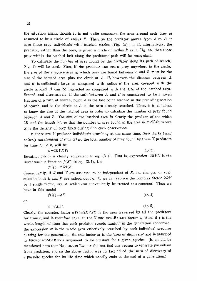
Suppose a number of prey individuals are scattered at random over a plane where

one predator searches with an average speed V, completely independently of the distribution of the prey individuals, from point A to B (see Fig. 4). The path of the

predator between A and B is assumed to be rectilinear, and all the prey individuals

in the plane remain stationary. (It can be shown that an irregular path may be as-

sumed without influencing the conclusion, or that there is no need to assume a stationary

distribution of prey individuals.) As in Fig. 4a, each prey individual has an area around

it within, and only within, which the predator can recognize the prey. To simplify

[" �9 �9 .

(a) (b)

Fig. 4. A geometric interpretation of the NICHOLSON-BAILEY (1935) model. For explanation see text.

26

the situation again, though it is not quite necessary, the area around each prey is

assumed to be a circle of radius R. Then, as the predator moves from A to B, it

sees those prey individuals with hatched circles (Fig. 4a) ; o r if, alternatively, the

predator, rather than the prey, is given a circle of radius R as in Fig. 4b, then those

prey within the hatched belt along the predator's path will be recognized.

To calculate the number of prey found by the predator along its path of search,

Fig. 4b will be used. First, if the predator can see a prey anywhere in the circle,

the size of the effective area in which prey are found between A and B must be the

size of the hatched area plus the circle at A. If, however, the distance between A

and B is sufficiently large as compared with radius R, the area covered with the

circle around A can be neglected as compared with the size of the hatched area.

Second, and alternatively, if the path between A and B is considered to be a given

fraction of a path of search, point A is the last point reached in the preceding section

of search, and so the circle at A is the area already searched. Thus, it is sufficient

to know the size of the hatched area in order to calculate the number of prey found

between A and B. The size of the hatched area is clearly the product of the width

2R and the length Vt, so that the number of prey found in the area is 2RVXt, where

X is the density of prey fixed during t in each observation.

If there are Y predator individuals searching at the same time, their paths being

entirely independent of each other, the total number of prey found by these Y predators

for time t, i. e. n, will be

n-:2RVXYt (4b. 3).

Equation (4b. 3) is clearly equivalent to eq. (3.1). That is, expression 2RVX is the

instantaneous function f ( X ) in eq. (3.1), i.e.

f ( x ) : 2 RVX. Consequently, if R and V are assumed to be independent of X, i.e. changes or vari-

ation in both R and V are independent of X, we can replace the complex factor 2RV

by a single factor, say, a, which can conveniently be treated as a constant. Thus we

have in this model

f ( X ) - a X (4b. 4)

o r

n =aXYt. (4b. 5).

Clearly, the complex factor aYt(=-2RVYt) is the area traversed by all the predators

for time t, and is therefore equal to the NICHOLSON-BAILEY factor s. Also, if t is the

whole length of time that each predator spends hunting in the generation concerned,

the expression at is the whole area effectively searched by each individual predator

hunting for the generation. So, this factor at is the 'area of discovery' and is assumed

in NICHOLSON-BAILEY'S argument to be constant for a given species. (It should be

mentioned here that NICHOLSON-BAILEY did not find any reason to separate parasitism

from predation, and so the above factor was in fact called the area of discovery of

a parasite species for its life time which usually ends at the end of a generation.)

Now, if the prey density in the present model is subject to decrease because of

predation, X should be replaced by variable x. Then eq. (4b. 4) becomes . f ( x ) = a x ,

which is identical to eq. (3.6) in every respect. Thus in conclusion we have eq. (3.8)

which is identical to eq. (4b. 2). The above discussion will be summarized below.

If the predator 's paths are independent of each other as well as of the distribution

of prey individuals, and also if the paths are deflected every now and then, predators

will sooner or later cross those paths already traversed by themselves or by others,

where the probability of finding still-undiscovered prey will be effectively nil, provided

that all the prey discovered are eaten. (If a proportion of prey in the area traversed

is not discovered, the predator 's effectiveness is reduced by lessening the effective

area of discovery by that proportion. If, however, this proportion is independent of

prey density, it does not influence the end conclusion.) Now, the paths intersect each

other more frequently as either the t ime spent hunting by each predator or the

number of predators hunting increases, and so the efficiency of finding prey drops

progressively.

This is the geometric meaning of 'competition' in NICHOLSON'S concept and is, as

already mentioned, synonymous with the 'law of diminishing returns' . The effect of

diminishing returns still exists even when only an individual predator is hunting.

The effect can still be called 'competition' since the predator is competing with itself,

so to speak. In this respect, the NICHOLSONIAN competition should be distinguished

from competition caused by social interference.

As already mentioned, the NICHOLSON-BAILEY model assumes animals with discrete

generations. Let us introduce this condition into the LOTKA-VOLTERRA eqs. (4a. la)

and (4a. lb) . As generations are discrete, no birth will take place during t in both

populations; the coefficient of increase for the prey species will never exceed zero,

i.e. r<0 . Also, the coefficient a ' for the predator species must be zero as no birth

takes place in this species either. Thus, we have

d x / d t = ( r - a y ) x

d y / d t = - r ' y

where r_<_O and r 'kO.

Let the initial density of the predator population be y0, then the second equation

yields y =yoe -''~.

Substituting the right-hand side of the above equation for y in the first equation, we

have

d x / d t = (r - ayoe- r,~) x,

and integrating

z = x0 [1 - e { r t - ayo (1 - e -r ' t ) / r '} ] (4b. 6)

(note that z = x o - x ) . Now, NmHOLSON and BAILEY ignored decrease in both prey

and predator populations caused by factors other than predation. This of course

means that both coefficients r and r ' tend to zero. Then eq. (4b. 6) becomes

28

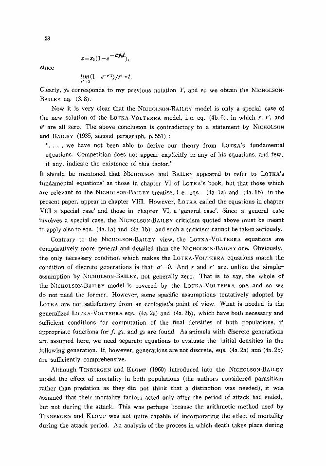
z =Xo (1 - e -ay~

since

l ira (1 - e - , ' t ) / r ' : t. r~-~O

Clearly, y0 corresponds to my previous notation Y, and so we obtain the NICHOLSON-

BAILEY eq. (3. 8).

Now it is very clear that the NICHOLSON-BAILEY model is only a special case of

the new solution of the LOTKA-VOLTERRA model, i.e. eq. (4b. 6), in which r, r ' , and

a' are all zero. The above conclusion is contradictory to a statement by NICHOLSON

and BAILEY (1935, second paragraph, p. 551) :

" . . . , we have not been able to derive our theory from LOTKA'S fundamental

equations. Competition does not appear explicitly in any of his equations, and few,

if any, indicate the existence of this factor."

It should be mentoned that NICHOLSON and BAILEY appeared to refer to 'LOTKA'S

fundamental equations' as those in chapter VI of LOTKA'S book, but that those which

are relevant to the NICHOLSON-BAILEY treatise, i.e. eqs. (4a. la) and (4a. lb) in the

present paper, appear in chapter VIII. However, LOTKA called the equations in chapter

VIII a 'special case' and those in chapter VI, a 'general case'. Since a general case

involves a special case, the NICHOLSON-BAILEY criticism quoted above must be meant

to apply also to eqs. (4a. la) and (4a. lb) , and such a criticism cannot be taken seriously.

Contrary to the NICHOLSON-BAILEY view, the LOTKA-VOLTERRA equations are

comparatively more general and detailed than the NICHOLSON-BAILEY one. Obviously,

the only necessary condition which makes the LOTKA-VOLTERRA equations match the

condition of discrete generations is that a ' - 0 . And r and r ' are, unlike the simpler

assumption by NICHOLSON-BAILEY, not generally zero. That is to say, the whole of

the NICHOLSON-BAILEY model is covered by the LOTKA-VOLTERRA one, and so we

do not need the former. However, some specific assumptions tentatively adopted by

LOTKA are not satisfactory from an ecologist's point of view. What is needed is the

generalized LOTKA-VOLTERRA eqs. (4a. 2a) and (4a. 2b), which have both necessary and

sufficient conditions for computation of the final densities of both populations, if

appropriate functions for f , gl, and gz are found. As animals with discrete generations

are assumed here, we need separate equations to evaluate the initial densities in the

following generation. If, however, generations are not discrete, eqs. (4a. 2a) and (4a. 2b)

are sufficiently comprehensive.

Although TINBERGEN and KLOMP (1960) introduced into the NICHOLSON-BAILEY

model the effect of mortality in both populations (the authors considered parasitism

rather than predation as they did not think that a distinction was needed), it was

assumed that their mortality factors acted only after the period of attack had ended,

but not during the attack. This was perhaps because the arithmetic method used by

TINBERGEN and KLOMP was not quite capable of incorporating the effect of mortality

during the attack period. An analysis of the process in which death takes place during

29

the attack period is now possible with the aid of the generalized LOTKA-VOLTERRA

eqs. (4a. 2a) and (4a. 2b).

The final point of investigation in this section will be concerned with the real

meaning of the 'area of discovery' in the NICHOLSON-BAILEY terminology, i.e. at, or

2RVt in my notation.

In the dynamics of gas molecules, the movement of a molecule can be regarded

as ideally haphazard and independent of other molecules before it collides with an-

other. Then the number of collisions that will occur during time interval At will be

2RVxAt in which R is the effective radius, V the average speed of each molecule,

and x the population density of the molecules. Clearly, the NICHOLSON-BAILEY model,

as well as the second term in LOTKA-VOLTERRA eq. (4a. la), is an analogy to the

'law of mass-action' in physical chemistry. (This was perhaps the reason by which

VOLTERRA justified his assumption of the linear relationship between the frequency

of encounters and the densities of prey and predator species.) The competition equa-

tion as expressed in eq. (3.8) is in fact identical to what is called in chemistry

the 'velocity equation for a unimolecular reaction'.

It is not difficult to visualize what the effective radius of a gas molecule is,

since it is the radius in which an effective contact with another molecule is made so

that a reaction takes place. However, what is the effective radius for a predator ?

NICHOLSON and BAILEY assumed that this was the radius within which a predator

could recognize the prey. However, for the competition equation to be an exact analogy

to the velocity equation, as the form of the NICHOLSON-BAILEY equation implies, the

path of a predator (a molecule) has to be completely independent of the position of

the prey (other molecules) immediately before the collision. In other words, the

predator's recognition of a prey has to be made, strictly speaking, by bodily contact.

If, however, recognition was made well away from the prey, the predator would have

to approach it, and this immediately means a digression from a free path. The problem

now is, how much deviation from the competition equation would be expected by

the digression from a free path. This degression can be serious under certain circum-

stances as will be discussed in w 4e.

Also, if it is assumed that recognition occurs at some distance from the prey,

the predator may see more than one prey individual at a time. Unless the pred-

ator can catch the prey in a sweeping action, each prey must be handled individually.

Under these circumstances, recognition will not result in immediate capture. In other

words, the number of prey that a predator can capture would not increase as fast as

the number of recognitions increases with increasing density of prey population.

This problem will be discussed in ~ 4d.

The last point, which is more important than any other, is the effect of the time

spent catching, killing, digesting, etc., for each victim. In the analogy of unimolecular

reaction, there is no need to think about the time involved in actions taking place

after a collision is made since each molecule ceases to capture more. In the predation

30

models, each predator continues to catch a number of prey during the period concerned.

While it is handling the victim, the predator temporari ly stops searching, and this

handling time should be separated from effective searching time. No doubt, as the

number of captures increases within a given period, the smaller is the proportion of

the period available for searching, and hence the number of captures increases only

asymptotically as the prey density increases (for details see w 4c).

It is clear that because of their neglect of some unavoidable physical properties

t h e N I C H O L S O N - B A I L E Y concept of the 'area of discovery' is quite unsatisfactory as a

basis of calculating the number of captures. The te rm may be used as one denoting

the efficiency of a predator 's catching activity now for a historical reason, but if so it

should be borne in mind that the te rm loses its geometric implication and becomes

only metaphorical.

The usage of the te rm 'area of discovery', widely seen in the literature of popu-

lation dynamics, is in fact of this metaphorical nature, because it is not an 'area'

measurable in physical dimensions. It is a value to be calculated from eq. (3. 7),

i.e. in the NICHOLSON-BAILEY model for predation,

at= 1 in Xo (4b. 7) X0 - - z

(note that X=Xo-Z), and for a special case of parasitism, i.e. in eq. (3. 23),

= + I n X (4b. 8). a t X - z

If we accept this metaphorical implication of the term, for historical reasons,

and redefine it as a calculated value in the right-hand side of eqs. (4b. 7) or (4b. 8), the

concept of 'area of discovery' becomes one way of expressing the hunting efficiency

(though not necessarily a useful one: see the appendix to w 4i), completely emanci-

pated from its original implication as a geometric measure of the effective area of

recognition (or catching) as in Fig. 4. Naturally, the value under the logarithmic

sign in eqs. (4b. 7) and (4b. 8) involves various factors which are of no geometric

significance, e.g. the t ime spent in activities other than searching, mortality in both

hunting and hunted species, and social interactions among the hunters.

In order to make a clear distinction between the two concepts : (1) ' the area of

discovery' as a measure of hunting efficiency, defined by the right-hand side of eqs.

(4b. 7) and (4b. 8), and (2) 'the effective area of recognition' as truly a geometric measure

in models appearing in this paper, I shall use, throughout this paper, a symbol /~ for

the former measure as distinguished from a plain symbol a for the latter. Thus, the

/~ for predation is :

i ~ = 1 In Xo (4b. 9), X0 - - Z

and the /~ for parasitism is :

i~ = ~ l n X (4b. 10). X - z . [

31

In this scheme, the NICHOLSON-BAILEY model is a particular case in which ii=-at

(constant). However, as will be shown in later sections (also summarized in the

appendix to w 4i), the value /~ cannot normally be constant but a function (and often

a decreasing function) of both predator and prey (or parasite and host) densities.

It should be recalled again here that the NICHOLSON-BAILEY model, although in

their paper used extensively as a model of para~ is essentially a predation model,

a special case of the LOTKA-VOLTERRA model. For the reason given in w 3, it turns

out to be of the same form as a parasite model only because the instantaneous hunting

function is assumed to be linear. This assumption is no longer reasonable, however.

c). HOLLING'S disc equation

HOLLING (1959b) performed the following simulation experiment. A number of

cardboard discs were placed on a table in a casual way. A blind-folded subject tapped

the table with a finger to discover discs, again in a casual manner. When a disc was

found, it was picked up and carried to a corner of the table, then a new series of

taps was performed to find another disc, and so on. After a series of experiments at

various disc densities, the number of discs handled in a given time was plotted against

the density of the discs. The curve thus obtained looked like that in Fig. 1, i.e. the

number of discs taken increased as the disc density increased but gradually leveled

off.

HOLLING'S explanation for this trend was as follows. It was assumed that the

probability of finding a disc with a tap was proportional to the density of the discs.

Thus, letting a be the proportionality factor, which HOLLING called the 'instantaneous

rate of discovery', and t, be the time spent tapping, the number of discs touched

(i.e. n) for t, would be

n=aXt, (4c. 1)

where X is the density of the discs. This evaluation is reasonable provided that the

disc density is kept constant during each experiment ; thus capital letter X is used

above. HOLLING, however, did not explicitly mention that X was kept constant to

meet this condition.

Now if an average time h was spent handling a disc each time one was found,

the total time spent handling n discs must be hn. Thus the total hunting time t (i. e.

total time tapping+total time handling) must be

t=t,+hn (4c. 2).

Eliminating t~ from eqs. (4c. 1) and (4c. 2) we have

n =aXt/(1 +ahX) (4c. 3).

This is HOLLING'S disc equation and describes his experiments very well. HOLLING

showed that this equation also fitted observed relationships in experiments with

various living predator and parasite species very well. Equation (4c. 3) clearly shows

that, because of the involvement of factor h, the number of prey captured by a

predator for a given time is limited, and under no circumstances can exceed l/h, since

32

lim n / t = l / h . X~co

(It should be mentioned in passing, however, that there is a logical jump from the

assumption of the disc model to the above conclusion (see w 4d).)

Although this model is excellent to demonstrate the effect of the handling t ime

upon the number of captures, the application of this model to various observations

with actual animals, by HOLLING himself and by others, is open to criticism. Let us

examine the disc experiment more critically below.

First, the assumption that the probability of finding a disc is proportional to the

density of discs is justified only when the discs do not overlap and only for as long

as the disc density is kept constant. Clearly, the mathematical probability of touching

a disc at a tap must, under these circumstances, be equal to the proportion of the

total area covered with the discs to the area of the table, provided that every part

of the table has an equal probability of being tapped. Hence, letting R, S, and X be

the radius of each disc, the size of the table, and the density of discs (fixed during

t in each set of experiment), respectively, the probability of discovery, P, at each tap

will be P=1rR~SX/S-TrR2X. As the frequency with which discs are touched (i. e. n)

for tapping t ime to must be the product of P, t~, and the frequency of tapping per

unit t ime (i. e. k), we have

n =Pkts

= ~R~Xkts (4c. 4).

Comparing eq. (4c. 4) with eq. (4c. 1), we find that HOLLING'S factor a, his instanta-

neous rate of discovery, is in fact ~R2k. As zc, R, and k can all be assumed to be

constant, factor a can also be constant.

Now, if eq. (4c. 1) is compared with eq. (4b. 5), it is clear that the former is a

special case of the latter; that is, t in eq. (4b. 5) is replaced by t~, and Y is set equal

to 1. Hence, HOLLING'S disc equation also applies to the NICHOLSON-BAILEY geometric

model as in Fig. 4. This means that HOLLING'S model seems reasonable if, and

perhaps only if, the predator is either a sweep-feeder or tap-feeder (such as plankton-

feeders or shore birds probing their beaks into the sand), but in either case discovery

of prey should be made by bodily contact. This implies that the size of the disc is

either the size of the body of the prey in the case of a tap-feeder, or the ambit of

the catching apparatus in the case of a sweep-feeder. Although both NICHOLSON-BAILEY

and HOLLING assumed that the factor s or a involves the distance at which the

predator perceives a prey (HOLLING 1961), the distance should be restricted, for the

reason raised above, only to a very limited area around the prey or the predator. If

this limitation is removed, the size of the disc should, in the case of the tap-feeder,

set the upper limit of the disc density, because the probability of discovery is zcR2X,

which should not exceed unity. This is somewhat artificial, and the problem will be

discussed in w 4d and e.

In HOLLING'S disc eq. (4c. 3), the number of predators searching does not explicitly

33

appear. This is perhaps because HOLLING used only one finger and also because n is

the number of discs removed per table. If, however, there are two fingers tapping

independently, the frequency of tapping, k in eq. (4c. 4), will be doubled provided

that there is no interference. In general, if there are Y fingers tapping per unit

area of the table we have, in place of eq. (4c. 1),

n =aXYG (4c. 5)

in which n is the number of discs removed per unit area rather than per table.

This generalization would not influence eq. (4c. 2), and so, eliminating t~, we get

n = aXY t / (1 + ahX) (4c. 6).

As the disc density has been fixed in the above model situation, eq. (4c. 6) is obvious-

lY an instantaneous equation comparable to eq. (3.1), in which

f ( X ) = a X / (l +ahX) (4c. 7).

Hence the overall hunting equation for predation, i.e. eq. (3.13), will be evaluated

by integrating

dx /d t = - a x Y / (1 + ahx) (4c. 8).

Thus we have

z =x0 (1 - e -~(rt-7~)) (4c. 9).

Equation (4c. 9) is an overall form of HOLLINC'S disc equation, taking account of the

effect of diminishing returns, and is thus comparable with the LOTKA-VOLTERRA and

the NICHOLSON-BAILEY equations. It is at once clear that the equation is a generalized

NICHOLSON-BAILEY model, or that the latter is a special case of the former in which

factor h - 0 (cf. eq. (3.8)). Equation (4c. 9) represents a surface in a Z-Xo-Yt co-

ordinate system, the shape of which is very much like that in Fig. 3a. A cross-section

parallel to the z - Y t plane shows the effect of diminishing returns similar to the

cross-section in the NmHOLSON-BAILEY competition surface (Fig. 2). The shape of

a cross-section parallel to the Z-Xo plane in HOLLING'S surface is, however, curvilinear,

unlike the NICHOLSON-BAILEY one which is rectilinear (see Fig. 2a). (It is difficult to

make the variable z in eq. (4c. 9) perfectly dependent : nevertheless the surface can

be drawn by assuming that Xo is the dependent variable and z and Yt independent

ones.)

If the disc model is applied to parasitism of the indiscriminate type, the right-

hand side of eq. (4c. 7) should be substituted for f ( x ) in eq. (3. 22). Hence, if the

fingers tap, for example, entirely at random, the function r will be the zero-term of

a POISSON series, and so we have

z = X ( 1 - e -a~/(l+ahz~) (4c. 10).

This also generates a surface similar to that in Fig. 3a.

My intention in generalizing HOLLING'S disc equation is in fact to point out three

mistakes commonly seen in the scattered publications in which the original disc equa-

tion was applied directly to observed data (see e .g . HOLLING 1959). First, the

density of the predators is not always 1. If eq. (4c. 3) is fitted to observed data in

which Yr the estimates of the factor a and h in the equation inevitably involve

34

the effect of Y. In order to show the point, let us assume that a and h in eq. (4c. 6)

are the true estimates of the factors originally defined, whereas those in eq. (4c. 3)

are superficial and are written a ' and h' respectively. Then the fit of eq. (4c. 3) to

data, which should be correctly fitted by eq. (4c. 6), means that

a'Xt/ (1 + a'h'X) = aXYt / (1 + ahX) and transposing we get

h'=h/Y+ (a ' -aY) /aa 'XY or

a'=aY/ (l + a X ( h - h'Y) ).

Thus, estimates a ' and h' not only change as the predator density changes but also

they are a decreasing function of the prey density, unless a'=aY and h'=h/Y. Fur-

ther, they are not independent of the units in which the densities of both populations

are measured. Hence, such estimates have no universal value.

Secondly, the depletion of prey or, in the case of parasitism, superparasitism,

often occurred in the observations. If eq. (4c. 3) is applied to such data, it is the

same as fitting the instantaneous equation to one of the cross-sections parallel to the

Z-Xo plane of the surface generated by eq. (4c. 9) in the case of predation, or eq.

(4c. 10) in the case of parasitism. Obviously, the curve of a cross-section parallel to

the Z-Xo plane, as in Fig. 3a, changes as Y or t changes, and therefore the estimates

for factors a and h should change accordingly. Again such estimates have no univer-

sal value.

The third point is concerned with a precaution that should be taken when prey

density is changed by changing the size of the experimental universe, a method often

adopted to obtain an extremely high prey density with relatively few individuals (e. g.

MORRIS 1963; HAYNES and SISOJEVIC 1966). If this is done, however, it should

be noticed that the predator density changes too. To assess z in this method, we

measure a cross-section of the surface which goes diagonally across the xo-Yt plane.

As far as I know, all the published literature in which HOLLING'S disc equation

is applied, involves at least one of the above three misapplications. Yet, the goodness

of fit is, in many cases, remarkably high. This is because the equation involves two

factors that are normally estimated from the observed relationships between z and

x0. That is to say, the nature of the estimation ensures that the resultant curve fits

the observation well. Hence, a good fit does not constitute verification of the theory.

In my opinion, the significance of HOLLING'S simulation experiment with discs

and tapping is to show the importance of the factor h, and this simple model is

sufficient to show that "the area of discovery", i.e. /i, cannot be independent of prey

or host density, as clearly deduced from eqs. (4c. 9) or (4c. 10). However, an application

of the original model as in eq. (4c. 3) to a situation in which the effect of diminishing

returns is obviously involved, is incorrect.

35

d). The IVLEV-GAusE equation

IVLEV (1955), in his study of the feeding ecology of fish, proposed an equation

and used it rather extensively for the analysis of predation processes. One of IVLEV'S

fundamental ideas which led him to the study of feeding ecology appears to have

emerged from his dissatisfaction with one of VOLTERRA'S assumptions that the number

of prey taken by predators is a linear function of the prey density. IVLEV wrote in

his book (pp. 20-21, English edition, 1961):

" . . . , according to VOLTERRA'S position, in the case of an unlimited increase in

the concentration of the food material, there must also be an unlimited increase in

the amount of the food taken. This 'unlimited' increase is a biological absurdity,

since each individual is only capable of consuming a strictly limited quantity of

food in each unit time."

This criticism led IVLEV to propose a new hunting equation in the following quota-

tion:

" . . . the actual ration of food eaten by the predator over a certain period of t ime

will, under favorable feeding conditions, tend to approach a certain definite size,

above which it cannot under any circumstances increase and which also corresponds

to the physiological condition of full saturation. Hence the mathematical interpret-

ation of the given law takes a form which has been used fairly widely in quanti-

tative biology and physical chemistry. If the amount of the maximal ration is taken

as b, then the relation between the size of the actual ration u and the density of

the prey population v must be proportional to the difference between the actual and

maximal rations and can be expressed by

du/dv =a (b- u), (4d. 1)

where a represents the coefficient of proportionality. Integrating this equation, we

get

u =b (1 - e -~') ." (4d. 2)

(The symbols are mine).

Although IVLEV'S criticism of VOLTERRA is a correct one, there appear to be some

ambiguities and confusions in the second statement quoted above. It is not clear

what IVLEV was aiming at in these equations, because of inadequate definition of the

symbols in the equations. As far as I know, it is not explicitly mentioned anywhere

in his book, whether eq. (4d. 2) represents an overall hunting equation or an instan-

taneous relationship.

IVLEV'S treatise covers a wide range of problems in feeding ecology, which

includes problems in natural population and competition between species feeding on

the same food resources. Needless to say, these problems cannot be solved unless

the depletion of the resources is considered ; the notion of 'competition' in the VOL-

TERRA-GAusE (as well as in the NICHOLSON-BA1LEY) line of thought would not have

emerged without this fundamental phenomenon, the depletion of some essential requi-

36

site, e.g. space and food. It should have therefore been of fundamental importance

for IVLEV to make his position absolutely clear; whether he was aiming at an overall

relationship, which includes the effect of depletion, or an instantaneous relationship,

in which the effect is not considered.

Having studied IVLEV's inference critically, I reached the conclusion that eq.

(4d. 2) is not an overall hunt ing equation. This conclusion would seriously influence

the value of IVLEV'S treatise, and therefore I should present the proof of this conclu-

sion in order to eliminate the possibility that my remarks are too critical.

In order to prove m y point, let us assume firstly that eq. (4d. 2) is an overall

hunt ing equation equivalent to z=F(xo, Y, t) in my sys tem presented in w 3. Thus,

under this hypothesis, IVLEV'S symbol u is equivalent to m y z, and obviously v cannot

be x. i t follows that v=xo, the initial prey density. Then eqs. (4d. 1) and (4d. 2)

become respectively

dz/dxo = a ( b - z) (4d. 1') and

z ~ b (1 - e - aXo ) (4d. 2 ' ) .

Now, according to IVLEV, Z approaches, over a certain period of time, the maximal

ration b. In the meantime, b mus t be a positive value, and it has to be independent

of x0, since otherwise eq. (4d. 2') will not be yielded by eq. (4d. 1'). However, since

x0 is any given initial density of the prey, it can take any positive value. Thus, we

can choose a value of Xo smaller than b. Under these circumstances, z can exceed

the value of x0, which suggests that the predators can eat more than supplied, and

this is of course absurd.

I t is clear that IVLEV's symbol u cannot be z, and therefore we have to give up

the hypothesis that eq. (4d. 2) represents an overall hunt ing equation. The second

alternative is therefore that u is the number of prey taken by a given number of

predators per unit area for a given period of t ime when the prey density is kept

constant; the equation represents an instantaneous relationship. Under this hypothesis,

u is equivalent to n, and it follows that v is X, a fixed prey density. Hence, f rom

eqs. (4d. 1) and (4d. 2) we have

d n / d X : a ( b - n) (4d. 1") and

n = b (1 - e -~x) (4d. 2").

Equation (4d. 2") has no contradiction as an instantaneous hunt ing equation, i.e.

n = f ( X ) Y t , if the factor Y t in eq. (4d. 2") is either unity or involved in the factor

b. The latter situation is a general one, and so we can wri te :

b~bYt .

So that we have n = b ( 1 - e -~x) Y t (4d. 3).

IVLEV, when fitting his eq. (4d. 2) to observations with some fish species (figure

1 of his book), stated that five young fish were introduced into a container and

allowed to feed for 1.5 to 2 hours. No mention was made, however, of either how

37

big the container Was or if the prey density was kept constant; though, judging from

his statement (chapter 2, p. 18 of his book) that "Food consumption was s tud i ed . . .

by estimation of the food left over out of the quantity given . . . . ", the prey density

was apparently not kept constant. Obviously, in the light of my analysis leading to

eq. (4d. 3), IVLEV's variable u must have been influenced by the size of container and

consequently the density of fish: more precisely, the size of container influence-~ the

density of fish, and consequently the coefficient b, if the density of food species was

kept constant to meet the condition required for describing the instantaneous relation-

ship. If the food species diminished gradually during the course of predation, the

estimates of both coefficients a and b obtained by fitting eq. (4d. 3), even though it

takes factors Y and t into account, would have been different between observations

with different predator density, simply because it amounts to fitting an instantaneous

equation to one particular cross-section of the hunting surface. Hence, these coeffici-

ents a and b estimated in IVLEV'S experiments are specific to these experiments and

have no universal meaning. This is the same criticism I raised in regard to HOLLINO'S

model. In order to eliminate the awkwardness pointed out above, it is necessary to

deduce an overall hunting equation. But before doing so, I shall examine in more

detail the reason why IVLEV'S instantaneous equation takes such specific form: although

eq. (4d. 3) has no apparent contradiction as an instantaneous hunting equation, the

justification for starting our inference from the differential eq. (4d. 1) is yet to be

rationalized.

IVLEV obtained his idea concerning eq. (4d. 1) from three existing equations

developed in physical chemistry and physiology. The first was an equation for uni-

molecular reaction. The velocity equation for a simple unimolecular reaction takes

the form

dx /d t = - a x

where x is the density of molecules at time t, and a the reaction coefficient. So,

letting x0 be the initial density of the molecules, we have

z =x0 (1 - e -~)

where z - - x o - x . As already seen, this is the NICHOLSON-BAILEY equation in which

Y=I . Of course, there is a resemblance between the velocity equation and IVLEV's

equation in their mathematical form, but the meanings are entirely different since

the derivative dx /d t in the velocity equation is the rate of change in time, whereas

d n / d X in IVLEV'S is the rate of change with density. These two attributes are,

needless to say, totally irrelevent to each other. Therefore, the quotation of the

velocity equation by IVLEV is absolutely irrelevant in his context.

IVLEV also quoted the "WEBER-FECHNER law" (but without citing the literature

source). As far as I know, this is a law in neuro-physiology representing the rela-

tionship between the strength of a stimulus and the reaction of a nerve. However,

there appears to be no possible resemblance between this law and IVLEV'S equation

in their mathematical forms.

38

The last one is MITSCHERLICH'S formula concerning the relationship between

plant growth and nutrient supply. MITSCHERLICH (cited by RUSSELL 1961) assumed

that a plant or crop should produce a certain maximum yield if all conditions were

ideal, but insofar as any essential factor is deficient there is a corresponding short-

age in the yield. Further, it is assumed that the increase of crop produced by unit

increment of the lacking factor is proportional to the decrement from the maximum,

thus

dn/dx=a(b-n) where n is the yield obtained when the amount of the factor present is X, b the

maximum yield obtainable if the factor was present in excess, and a is constant.

While it may be understandable that IVLEV quoted MITSCHEgLmH'S equation,

since prey density can, in a way, be compared to the nutrient supply in plants, the

comparison is more like a metaphorical juxtaposition and does not really aid his

argument in predation. IVLEV'S failure to recognize the distinction between the overall

and instantaneous relationships, and also to incorporate the factors Y and t, implies

that such comparisons did not give a sufficient insight into the structure of predation.

Also, as already mentioned, there will be a number of mathematical equations which

can equally well describe the trend of the hunting curve that IVLEV obtained for

fish predation (figure I of IVLEV'S book). For instance, HOLLING's disc equation

shows a very similar trend, yet the meaning of the equation is quite different from

MITSCHERLICH'S formula. As I have shown in w 3, the formulation of a differential

equation in predation models has a definite significance as a means of inference. That

is, it is often an instantaneous relationship, between the components concerned, that

is self-explanatory and so can be formulated intuitively and correctly. IVLEV's equa-

tion, however, appears not to have been developed theoretically, but has been borrow-

ed by metaphor from other fields in which the development of a differential equation

has no relevant significance to predation.

It is, however, true that IVLEV'S equation has a remarkable descriptive power.

It might therefore be that some essential meaning or some fundamental structure of

predation processes is reflected in the equation. To find this out, the following sim-

ulation experiments will be considered.

Suppose a set-up similar to the disc experiments by HOLLING. The only difference

is that the distribution of the discs is ideally at random, and hence the discs may

overlap each other. To make calculation easier, however, the model is slightly modified,

though the principle of the model process remains unaffected. I t will be assumed that

the prey individuals are particles and a predator has a ring of radius R around itself.

Then, the ring, representing the recognition zone of the predator, is tossed over the

hunting area (a table), again at random; it should be strictly at random so that every

part of the table has an equal chance of receiving a toss of the ring.

Under these circumstances, the total number of particles (written as n~) falling

within the ring after a number of tosses will be in proportion to the density of the

39

particles. As the average number of particles within the ring is 7rR2X and the

number of tosses in time ts is kt,, where k is the frequency of tosses per unit time,

the total number caught by the ring will be

n~ =~R~kXt~.

Although the right-hand side of the above formula is the same as in eq. (4c. 4)

describing HOLLING'S experiment, notation n, in the left-hand side is not n as in eq.

(4c. 4). It was assumed in HOLLING'S model that all the discs tapped were taken,

and it was a justifiable assumption since only one disc was discovered at a time as

there was no overlap of the discs. In the present model, however, more than two

particles may occur within the ring at one toss. Thus, if the predator is allowed to

catch only one prey individual within its recognition zone at a time, the total number

captured (i. e. n) will be the number of successful tosses rather than ns, the total

number discovered.

In the present model, the distribution of the prey individuals and the tosses of

the ring are ideally at random, and so, provided that R is not too large as compared

with the table, the frequency of tosses in which a given number of particles falls

must follow a POISSON series with its mean equal to the average number of particles

in the ring at one toss, i.e. rcR~X. Hence, as the frequency with which no particle

occurs within the ring in the period t, will be kt,e -~R*X the total frequency of

successful tosses in t, will be

n =kt, ( l - e - ~R~X ).

In the above model, only one ring was assumed to be tossed at the frequency of k

per unit time per table. If there are Y rings per unit area tossed independently,

each at the average frequency of k per unit time, the total frequency is kYts, and

so the above equation becomes

n=kYt~(1 -e -'~R~X ) (4d. 4).

If kYt~ in the above equation is set equal to b, and rcR 2 to a, we have IVLEV'S eq.

(4d. 2"). Thus, we find that IVLEV'S equation, in terms of the toss-a-ring simulation,

is a generalized version of HOLLING'S experiment, since eq. (4d. 4) is a generalization

of eq. (4c. 5). That is, recognition zones can overlap, and so there is no restriction

to the range of variation in the prey density X (remembering that HOLLING'S eq.

(4c. 5) holds in the disc experiment only for X<I/=R2).

Now, eq. (4d. 4) suggests that the amount of ration per unit time per predator,

i.e. n/Yt~, can under no circumstances exceed the value of k. That is, the number

captured is limited by the frequency of tosses but not by the factor h as in HOLLING's

concept, which is not yet considered in the toss-a-ring experiment. The frequency of

tosses is of course equivalent to the frequency of taps, and therefore the factor k is

in fact involved in HOLLING'S disc experiment too. However, in HOLLING'S experi-

ment, the maximum ration is obtained when the prey density reaches 1/~R 2, because

of the limitation that r:R2X should not exceed unity, since it is the probability of

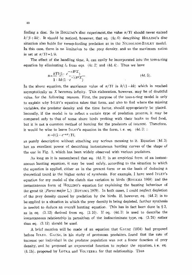
40

finding a disc. So in HOLLING's disc experiment, the value n/Yt should never exceed

k/(l+hk). It should be noticed, however, that eq. (4c. 6) describing HOLLING'S disc

situation also holds for sweep-feeding predation as in the NICHOLSON-BAILEY model.

In this case, there is no limitation to the prey density, and so the maximum ration

is set at n/Yt~l/h. The effect of the handling time, h, can easily be incorporated into the toss-a-ring

equation by eliminating t~ from eqs. (4c. 2) and (4d. 4). Thus we have

kYt( l_e -~R2X) (4d. 5).

n=l + hk( l_e- ~R2x )

In the above equation, the maximum value of n/Yt is k/(l+hk) which is reached

asymptotically as X becomes infinity. This elaboration, however, may be of doubtful

value, for the following reasons. First, the purpose of the toss-a-ring model is only

to explain why IVLEV'S equation takes that form, and also to find where the missing

variables, the predator density and the t ime factor, should appropriately be placed.

Secondly, if the model is to reflect a certain type of predation process, it may be

compared only to that of some shore birds probing with their beaks to find food,

but it is not a common method of hunting for the predators of interest. Therefore,

it would be wise to leave IVLEV's equation in the form, i.e. eq. (4d. 3) :

n = b (1 - e -~x) Yt, as purely descriptive without attaching any serious meaning to it. Equation (4d. 3)

has an excellent power of describing instantaneous hunting curves of the shape of

the one in Fig. 1, which has been widely observed with various predators.

As long as it is remembered that eq. (4d. 3) is an empirical form of an instant-

aneous hunting equation, it may be used safely, according to the situation to which

the equation is applied, either as in the present form or as the basis of deducing a

theoretical trend in the higher order of synthesis. For example, I have used IVLEV'S

equation for my model of the clutch size variation in birds (RoYAMA 1969) and the

instantaneous form of HOLLING'S equation for explaining the hunting behaviour of

the great tit (Parus major L.) (ROYAMA 1970). In both cases, I could neglect depletion

of the prey density caused by predation by the birds. If, however, eq. (4d. 3) is to

be applied to a situation in which the prey density is being depleted, further synthesis

is needed to deduce an overall hunting equation. This has in fact been done in w 3,

as in eq. (3. 12) derived from eq. (3.10). If eq. (4d. 3) is used to describe the

instantaneous relationship in parasitism of the indiscriminate type, eq. (3. 24) rather

than eq. (3.12) should be used.

A brief mention will be made of an equation that GAUSE (1934) had proposed

before IVLEV. GAUSE, in his study of protozoan predators, found that the rate of

increase per individual in the predator population was not a linear function of prey

density, and he proposed an exponential function to replace the equation, i.e. eq.

(4. lb) , proposed by LOTKA and VOLTERRA for that relationship. Thus

41

(dy/dt)/y = C ( 1 - e-~) (4d. 6)

where C and ,t are positive constants. I shall examine in the following: (1) whether

GAUSE'S proposal of eq. (4d. 6) is acceptable, and (2) why the right-hand side of eq.

(4d. 6) takes the same form as that of IVLEV'S eq. (4d. 2 ' ) .

Although GAUSE was aiming at the formulation of the relationships between a

protozoan predator and its prey, his experimental justification of eq. (4d. 6) came

from an observation by ~MIRNOV and WLADIMIROW (cited by GAUSE 1934, pp. 139-140)

of a parasite, Mormoniella vitripennis, attacking its host, Phormia groenlandica. It

should be remembered that the relationship expressed in the form of a differential

equation as in eq. (4d. 6) will not be appropriate in the case of an entomophagous

parasite in which generations are discrete. This is because, while the expression

C ( 1 - e -~*) stands for the number of progeny (per unit area) produced per parasite

during t in the present generation to form the next generation, these progeny will

not reproduce in the present generation. Therefore, it is incorrect to equate the (dy/

dt)/y to C(1-e-~*). Before making further comments on eq. (4d. 6), however, I shall

investigate the second point, i.e. why were changes in the density of the parasites'

progeny, in relation to changes in host density as observed by SMIRNOV and WLADI-

MIROW, described by the formula C ( 1 - e -~) which is of the same form as IVLEV'S ?

Let Y' be the density of progeny in the parasite population produced to form the

next generation, and z the density of hosts attacked in the present generation. Let

us assume hypothetically that Y' is more or less proportional to z, i.e. Y'=c'z where

c' is a proportionality constant. In the meantime, it has been shown that although it

is an instantaneous equation, eq. (4d. 3) can nevertheless describe one cross-section,

parallel to the z -X plane, of an overall hunting surface for parasitism, e. g. eq.

(3.22). In other words, although eq. (4d. 3) should correctly be used to estimate the

value of n, the equation can, because of its considerable flexibility in fitting, also

describe the z -X relationship, provided that the coefficients a and b are appropriately

chosen for a given value of Yt, i.e. for a given cross-section of the hunting surface.

Under these circumstances, one may obtain, though only superficially,

Y'=c'b(1-e -ax) Yt,

or by transposing Yt to the left-hand side,

Y'/Yt =c'b (1 - e -ax) (4d. 7).

In the SMIRNOWWLADIMIROW observation, as presented in figure 40 of GAUSE'S

(1934) book, the factor Yt appears to be fixed at the same value for different values

of X throughout the observation, and this consistency satisfies the condition under

which eq. (4d. 7) has been derived. Clearly, the expressions Y'/Yt and X in eq.

(4d. 7) are equivalent to (dy/dt)/y and x respectively in eq. (4d. 6), and the constants

c'b and a in eq. (4d. 6) can be written as C and 2 respectively as in eq. (4d. 6).

And this is why GAUSE's equation can be deduced from IVLEV'S.

The reasoning which led to eq. (4d. 7) explains why GAUSE adopted eq. (4d. 6),

and also why GAUSE and IvLgv proposed the same function, though GAUSE was

42

thinking of a function equivalent to g2 in eq. (4a. 2b) while IVLEV was thinking of

one equivalent to the function f in eq. (4a. 2a). This reasoning suggests, however,

that GAUSE'S propgsal of his equation, the justification of which was based erroneously

on an observation of parasites with discrete generations, is not acceptable, for two

reasons, if applied to predators with continuous generations. First, as pointed out by

NICHOLSON and BAILEY (1935, p. 552, first paragraph), the number of progeny in a

predator population, unlike that in a parasite population, will not in general be propor-

tional to the number of prey eaten by the parental predators. This objection might

be avoided if it could be verified that the exponential function as in eq. (4d. 6) still

holds for protozoan predators in which the value and the ecological significance of

the coefficient ~ are different from those of the coefficient a in eq. (4d. 7), and there-

fore that the similarity between the two equations is only coincidental.

My second objection, however, seems unavoidable. Clearly, dy/dt is a linear func-

tion of y in eq. (4d. 6), suggesting that the predator population exhibits a geometric

increase for any given value of x. This contradicts GAUSE'S own suggestion of a

logistic law with respect to the natural increase of the prey population in the absence

of predators; in particular with respect to the function gl (x) in the generalized LOTKA-

VOLTERRA eq. (4a. 2a). GAUSE'S inconsistency in this respect, i.e. adopting the logistic

law for gl and neglecting it for gz, appears to be attributed to the misconception in

his statement (GAuSE 1934, p. 53, last paragraph): "In the general form the rate of

increase in the number of individuals of the predatory species resulting from the

devouring of the prey dN2/dt Eequivalent to dy/dt in my notation] can be represented

by means of a certain geometrical increase which is realized in proportion to the

unutilized opportunity of growth. This unutilized opportunity is a function of the

number of prey at a given moment." It appears that GAUSE overlooked in the last

sentence above that the 'unutilized opportunity of growth' in the predator population

is a function not only of the density of prey but also of the density of the predators

at the same time.

To summarize, in section IV of chapter III in his book, GAUSE (1934) tried to

improve the LOTKA-VOLTERRA formulation of the prey-predator system. His sugges-

tions, however, were reasonable only with respect to the function gl (x) in eq. (4a. 2a)

and not with g2(x, y) in eq. (4a. 2b). As to the function f(x, y) in eq. (4a. 2a),

there was no suggestion by GAUSE, and the function f was left uncriticized as a

linear function of x, which is unreasonable. For these reasons, GAUSE'S mathematical

investigations into the prey-predator interaction system are unsatisfactory.

e). ROYAMA'S model of random searching and probability of random encounters

In the previous sections, it has been shown that the instantaneous hunting func-

tion, i. e. f , is, unlike the simple assumption by LOTKA and VOLTERRA and by

NICHOLSON and BAILEY, not a linear function of prey or host density. This finding

influences the notion of 'the area of discovery' that was originally used by NICHOLSON

43

and BAILEY but redefined in w as /~=(1/Y) In{xo/(Xo-Z)} for predation, and / i=

( l /Y) ln{X/(X-z)} for parasitism. If the instantaneous function f (x ) i s a non-linear

function, z is also a non-linear function of x0 or X, and hence /~ cannot be constant.

Although the models proposed by HOLLING and IVLEV, reviewed in w 4c and d, are

adequate to show that /~ will not be constant theoretically, these models are not quite

sufficient to show how /~ can logically vary. One of the key points for this analysis

seems to lie in understanding the coefficient a (not /~).

The coefficient a appeared consistently in the instantaneous hunting function of

models reviewed in preceding sections, with the same geometric meaning, namely the

size of an area immediately around either a prey or a predator individual within

which the predator would take action to catch the prey. In all the models, it was

assumed that the coefficient a was constant, or independent of variables x, y, and t.

Some objections arose among ecologists (see below) against the validity of the assump-

tion that the coefficient was constant,

yet. The main purpose of the present

nature of this coefficient.

The justification of the assumption

and the debate has not quite been settled

section is to give a much clearer idea of the

that a is constant is partly concerned with

the validity of the assumption of random searching--whether or not such an assumption

is reasonable in predation or parasitism theories. The idea of random searching and

random encounter is not new. It has been used very widely among theorists, and

while the concept of randomness is clearly defined in the field of mathematics,

confusion has resulted from loose application of the concept to an ecological situation.

First, one must separate the concepts of random searching and random encounters, as the one does not necessarily follow the other. Perhaps the most satisfactory defini-

tion of the te rm 'random searching' is that the path of each individual predator is

affected neither by the location of prey individuals in the hunting area nor by the

paths of other members of the predator population. 'Random encounter', as opposed

to ' random searching', can be defined as meaning that every prey individual in the

area concerned has an equal probability of being encountered by predators searching

for a limited t ime interval. Now, the simple theory of the kinetics of gas molecules,

used by LOTKA, VOLTERRA, and NICHOLSON and BAILEY, assumes random encounters

between molecules, and so the theory can be a model for random searching to a

limited extent. This is because, as pointed out earlier, the analogy can be reasonably

applied to hunting behaviour only when an encounter is made by bodily contact;

otherwise, random encounters are approximately guaranteed only if either (1) the

number of predators searching independently is high, (2) the t ime for searching is

unlimited, or (3) the density of prey is relatively low.

This can be illustrated by assuming that a few molecules are marked as predators,

and all other molecules, unmarked, are prey. Then the movement of these few marked

molecules for a certain limited t ime interval must be limited to a small fraction of

the total area concerned, so that the unmarked molecules located in the immediate

44

vicinity of any one of the marked molecules must have higher chances of being

encountered by the marked ones than those located remotely. However, if the number

of marked molecules is high, all the unmarked molecules have an equal chance of

being encountered by any of the marked one~.

LAING (1937) and ULLYETT (1947) were aware of a part of the above point and

stated, in their crit icism of the NICHOLSON-BAILEY theory based on random searching,

that a predator or a parasite can perceive the location of prey or host at a certain

distance away from it ; the search therefore can only be at random (a free path or

undirected path would be better words for random searching : my comment) as long

as the predator or parasite remains outside this zone of p e r c e p t i o n ; a s soon as it

enters this zone, its actions cease to be random and become, instead, directed towards

the prey or host. THOMPSON (1939) thus wrote that a theory that equates animal

action and random action covers at least only a fraction of the field, and that any

theory based on the assumption that search is random cannot be accepted as a valid

general theory.

Although these crit icisms sound reasonable, no at tempt has been made, as far

as I am aware, to find what and how much bias might be involved in a theory based

on random searching as against the more likely situation raised by the above authors.

I investigated this problem to some extent in a previous paper (RoYAMA 1966), but

because it was written in a language not normally accessible to English-speaking

readers, and also because I have since found some mathematical errors in it, all the

points will be revised here.

The investigation will be made with a situation in which a predator recognizes a

prey from some distance. For the moment, it is assumed that only one predator is

searching and that the prey density is kept constant. Suppose a number of particles

of kind P (prey) are scattered at random over a sufficiently large plane (a two-dimen-

sional space), each particle being given a circle of radius R as the recognition radius.

One particle of another kind Q (a predator) can recognize P only within the area

covered by the circles, so that Q's path is undirected when Q is outside the recogni-

tion area, but it is directed towards the nearest P within the recognition area. For

simplicity, it is supposed that all P ' s remain stationary, but that Q moves around in

the manner described. Also the radius R is the same for each P (although this as-

sumption is not quite essential). At the moment, the time spent handling P ' s after

they are caught by Q is not considered.

Now, the start ing point of Q will be determined on the plane at random. Then

one or other of the following two cases wilt occur (see Fig. 5). Case 1: the start ing

point happens to be outside any of the circles of P's. Then Q determines the direction

of its movement at random and moves along a (straight) free path until it contacts

a P ' s circle; then goes to the centre of the circle to capture the P. Case 2: the start-

ing point happens to be within one of the circles. Then Q immediately goes to the

nearest centre, where the P is located, along the shortest path. A situation is first

45

Fig. 5. ROYAMA'S first geometric model in which a predator (Q) recognizes its prey (P's, black dots) within a circle around each P, and searching by Q is discontinued each time a P is captured. A starting ponit (cross) is determined at random for each new search. For further explanation see the text.

cons idered in which Q discont inues searching each t ime it captures a P, and so the

nex t s t a r t ing point is de t e rmined again at r andom over the plane. Th i s is perhaps

comparab le to a b i rd col lect ing food for i ts young, and each t ime a food i tem is found

it is t aken to the nest, and the next hunt ing s ta r t s independent ly of the previous

search.

Suppose n of P ' s were caught by Q dur ing the total t ime spent in searching, ts,

(note tha t t h e number caught can be smal le r than the n u m b e r seen). Let n~ be the

n u m b e r of occur rences of case 1, L1 the average dis tance that Q t ravel led be tween

the s t a r t ing point outs ide any circle and the pe r iphe ry of the first c ircle tha t Q hap-

pened to encounter , and G the average speed of m o v e m e n t while Q was on an undi-

r ec ted path. S imi lar ly , let n2 be the number of occur rences of case 2, L2 the average

d is tance be tween the s ta r t ing point inside the c i rc les and the neares t cent re of the

circles, and Ve the average speed of m o v e m e n t along a d i rec ted path. Then we have

the fo l lowing fo rmula

ts = ( L1/ VI +R/V2) nl q- ( L2/ V2) ne (4e. 1).

Now, let Pr{n f f and Pr{ne} be the probabi l i ty tha t cases 1 and 2 occur respect ive ly ,

then

m = n P r { n , }

n2 = nPr {n2},

but s ince n l+n2=n ,

n2 = n ( 1 - P r {nd) ,

and so eq. (4e. 1) becomes

46

t ,=[ (LJV~ + R/V2) Pr {nl} + L2(1-Pr{n~} ) /V2]n (4e. 2).

Therefore, if L~, L~, and Pr{nl} are evaluated as functions of the density of pts (i. e.

X) , n can be determined as a function of X. Details of the evaluation of L1 and

L2 will be given in Appendices 1 and 2 respectively, and the end results alone will

be shown below:

L1 = 1/2RX (4e, 3) and

L2= {$(V'2rcX R ) / 1 / X - R e ,R X }/(1--e ,,R X ) (4e. 4)

where $ ( 1 / 2 ~ X R ) = ~ 2 ~ f ~ R e -02/2d0"

Now if we assume a sufficiently large area, the probability of Q's starting point

happening to be outside any of the circles of P's must be the 0-term of a PomsoN

series with its mean zcReX. Thus

- ~ r R 2 X Pr {Ytl} =e (4e. 5).

Eliminating L~, L2, and Pr{n~} from eqs. (4e. 2) to (4e. 5) inclusive and solving with

respect to n, we have - ~r R ~ X

n=[2RV~ V2/{V2 e +2R V ~ / X ~(v~2rcXR)} ]Xt8 (4e. 6).

Now, if there is Y number of Q's per unit area, the total number of P's caught will

be obtained simply by multiplying the right-hand side of eq. (4e. 6) by II, since the

equation is an instantaneous one. So, if the expression in the outer brackets on the

right-hand side of eq. (4e. 6) is denoted by a function a(X), where a is a functional

symbol, we have

n = a ( X ) XYt, (4e. 7).

Equation (4e. 7) is clearly comparable to eq. (4b. 5) in the NICHOLSON-BAILEY model

(note that in the NICHOLSON-BAII.EY model there is no distinction between t and ts)

and is also comparable to eq. (4c. 5) in HOLLING'S model. That is to say, the coeffi-

cient a for the two models is in fact comparable to the function a(X) in my model.

Now, it is clear that the coefficient a can no longer be considered to be independent

of X if a predator recognizes a prey from a distance and has to approach to seize it.

The new coefficient a(X) is normally a decreasing function of prey density. (It should

be noticed that the coefficient a in the NICHOLSON-BAILEY model is equal to 5 per

unit time, but neither the a in HOLLINa'S disc model nor a(X) in eq. (4c. 7) is /i

per unit time.) Let us examine the nature of a(X) more closely.

If the density of P ' s (i. e. X) is very low, then

lim a(X)=2RV1. X+O

So, if R and 171 are independent of X, eqs. (4e. 6) or (4e. 7) converges with the NICHOLSON-

BAILEY equation (cf. eq. (4b. 3)), or with HOLLISG'S before the introduction of the

factor h. This is reasonable because, if the prey density is low, a large part of the

predator 's movement should be undirected and therefore independent of the location

of prey individuals, in which case the analogy of unimolecular reaction is approxi-

47

mately true. Consequently, HOLLING'S disc equation should be a good approximation

for low prey densities.

On the other hand, if X is very large, then

lira a(X)=lim 2V~/v'X. X~o~ X~oo

Thus, when X increases, a (X) decreases in inverse proportion to the square root of

X. This is because the probability of any one P being found in the recognition

radius of a O increases as X increases, and so in its extreme situation, the movement

of the Q is largely governed by the location of P's. Under these circumstances, the

movement of the Q can no longer be independent of the location of P's. More

precisely, if the Q is most attracted to the closest one of the P's found in the recog-

nition area, then O's path consists largely of the distance to the closest P. As already

demonstrated by MORISITA (1054) and CLARK and EVANS (1954), the distance between

an arbitrarily selected point and the closest one of a number of randomly distributed

points in a two-dimensional plane is inversely proportional to the square-root of the

density of the random points. The same conclusion applies when the recognition

radius R is large relative to X. This suggests that HOLLING'S disc equation would

show its bias, even if X is low, when R is very large. Conversely, if R is comparatively

small, the disc equation is again a good approximation even if X is high. That is to

say, the equation holds whenever the R is reduced to an immediate area around the

prey so that a capture is made practically by bodily contact, and this confirms my

previous conclusion.

It should be pointed out, however, that the inverse proportionality of a(X) to

the square-root of X holds only when the hunting area is a two-dimensional plane.

If the hunting area is one-dimensional, such as thin branches of a tree, a (X) is in-

versely proportional to X ; a n d if it is a three-dimensional space, a(X) is inversely

proportional to the cubic-root of X (for the proof, see CLARK 1956).

The above investigation suggests that if HOLLING'S disc eq. (4c. 6) is applied to

my present model, the coefficient a thus estimated will show a decreasing trend as X

increases. MORRIS (1063) applied the disc equation to the instantaneous hunting curve

observed with Podisus maculiventris (Hemiptera) eating larvae of Hyphantria cunea (Lepidoptera). (MORRIS kept the density of the prey constant during the observation

to meet the condition for an instantaneous hunting curve.) It was found that, when

the factor h was assumed to be constant, the factor a decreased as the prey density

was increased. MORRIS thought that this was due to satiation by the predator. While

this interpretation is reasonable, it is equally tenable that the trend observed was due

to a decrease in the factor a as in my a(X). Hence, it is not known, unless the

experiment is designed accordingly, to what extent the trend is attributable to satiation

and to what extent to the geometric property of the hunting behaviour.

MILLER (1960) pointed out that both HOLLING'S and WATT'S equations (to be

reviewed in the next subsection) tended to deviate from the observed trend in various

48

animals when the prey densities were increased. My factor a (X) suggests that in

the case of parasitism, in which satiation might not be important, a deviation from

the observed would become greater as host density became higher.

Now, the handling-time factor h can be incorporated into my model by eliminating

t~ from eqs. (4c. 2) and (4e. 7), i.e.

n = {a (X ) X Y t } / { 1 + a (X ) hX} (4e. 8).

Some interesting characteristics are observed in curves generated by eq. (4e. 8).

The shape of the curves will change with changes in the ratio between the speed of

the predators' undirected movement and directed movement (see Fig. 6). As pointed

out already, eqs. (4e. 6) or (4e. 7) has two asymptotes, the one for X-~0 where n approac

2RVI Xt , , a straight line passing through the origin of the n - X coordinates; and the

other for X~oo where n-~2V~v 'Xt , . Therefore: (1) If the speed of undirected move-

ment is not lower than that of directed movement, i.e. V~ > V~, the curve generated

by eq. (4e. 8) will be a monotonically increasing one with its tangent ever-decreasing;

this is very much like the curve generated by HOLLING'S or IVLEV'S equations. (2) If

Va is considerably smaller than V2, the curve may be a gentle sigmoid. (3) If V1

and V~ have a certain ratio, the curve may be approximately linear for a wide range

of the prey density, in which case NICHOLSON-BAILEY'S model, rather than HOLLING'S

or IVLEV's, could be a better approximation (the Iinearity must sooner or later break

down as X increases, however). All of these trends have been observed with living

predators and parasites (see e.g. HOLLING 1959a). Equation (4e. 8) would not,

however, generate very strongly sigmoid curves. A probable mechanism which causes

such a strong sigmoid form has been discussed elsewhere (RoYAMA 1970).

R= 2 v2-- 200

h = 0.0'1

(~) V~ = 600 {2) = 50

{3) = 1 0

Fig. 6. Three examples of curves generated by eq. (4e. 8).

:~X

Now, from eqs. (4e. 8) and (3. 4), we have

d x / d t = - a (x) x Y / {1 +a (x) hx} ,

and so the overall hunting equation for predation is obtained by integrating the above

differential equation, i.e.

Yt = (1/2R V1) [ln (nR 2x) - nR 2x + (nR 2x) 2/2.21 - (nR ~x) 3/3.3 ! + . . . . ]xo

49

- - - - rr R ~ x X o + (l/V2) [2fO(V'2rrxR)l/x + (e )/rrR] x +h(xo-x) (4e. 9)

(the expression [ f (0)]0 0~ reads f(Oo) -f(O)).

Although I am unable to solve eq. (4e. 9) with respect to z : x o - x , the hunting surface

on the Z-Xo-Yt coordinate system can be calculated numerically with a computer.

Incidentally, the numerical values for the normal (or GAUSSIAN) integral ~ in eq.

(4e. 4) can easily be obtained from a table of the normal (or GAUSSIAN) probability

function.

Surfaces generated by eq. (4e. 9) will almost certainly fit a wide variety of hunting

surfaces actually exhibited by various predators, since the equation has four (rather

than two as in HOLLING'S and IVLEV'S ones) independent coefficients, R, V,, Vz, and

h, to be estimated from the observed surfaces. This suggests that a close fit does

not prove anything, unless the coefficients are measured independently and directly

in separate observations, which at the moment is technically difficult. However, the

model was designed primarily to show what degree of deviation of a(X) from the

constant a in simpler models could be expected. No at tempt was therefore made to

fit the equation to any observed data.

Another inquiry by a similar model will be made, secondly, into a situation in

which a predator or a parasite continues to hunt without leaving the area each t ime

a victim is captured, so that the starting point of a new path of search is the place

where the previous victim is captured. This situation is too complex to handle with

an analytic (mathematical) method, and so a Monte Carlo simulation has been used.

Two hundred points, representing prey, were plotted at random on a sheet of

graph paper (30• each point being given a circle of 2cm in radius. The

predator 's starting point was determined also at random. The direction of walk was

then determined again by chance with predetermined probability of occurrence; five

angles measured f rom a reference line, which was the previous path except for the

starting point, i.e. 0, • and • were given an equal chance of occurrence (a

backward movement with reference to the immediately previous path was excluded).

When the predator had moved up to the periphery of a circle, it went to the centre,

and the point was removed permanently from the area. If a second point was within

the 2-cm recognition radius from that point, the predator went straight to the second

one to catch it. If another point was not within 2cm, the predator determined its

direction in the manner described above, and carried on. A part of this simulation

experiment is shown in Fig. 7. The number of points removed is plotted on the

horizontal axis against the distance traversed by the predator on the vertical axis

(Fig. 8).

If we assume an equal speed of movement for the undirected and the directed

paths (i. e. VI= Vz), the distance traversed, L, per unit area is the product of the

speed of movement and the predator-hours. Thus, if VI~V2=I, then L=Yt, . Also

the effect of handling t ime is not essential in the present discussion and so is not

50

Fig. 7. I{OYAMA'S second geometric model in which predator Q continues to search for prey without shifting the starting point after each capture. Other features are the same as in Fig. 5.

200

(3 LI.I

0 ~E h l r,."

U") I.I.I

~.~ 100 I'-- n "

I.L 0

6 Z

R= 2CN

I I f I I I

I00 200 300 400 500 600

DISTANCE TRAVERSED (CM)

~ . _ - -

Fig. 8. An observed relationship (solid line with black dots) between the number of prey taken (vertical axis) and the distance traversed by a predator (horizontal axis) in a Monte Carlo simulation of the predation model of continuous search (cf. Fig. 7). The broken curve is generated by eq. (4e. 9) for R=2, 12"1=1, and h=0 as in the present Monte Carlo simulation. For details see text.

considered; thus L = Yr. So the horizontal axis in Fig. 8 is equivalent to the Yt-axis

i n Fig. 2a, and the vertical axis is of course the z-axis . Thus the graph in Fig. 8 is

equivalent to a cross-section in which x 0 = 2 0 0 / ( 3 0 x 3 9 ) parallel to the z-Yt plane in

Fig. 2a, i .e . it is a competit ion curve in the NICHOLSON-BAILEY sense.

T h e curve with solid circles is not monotonic but wavy , and there is a clear ten-

5T

dency towards a number of miniature waves. The explanation of this trend is rather

simple. As the direction and the length of each path are determined by chance, the

predator's track is a kind of MA~KOV'S chain, although the probability distributions

of both the direction of directed paths and the length of all paths are dependent

stochastically on the location of the prey which were encountered�9 This is a complex

(or a generalized) 'random walk'�9 Thus the predator's path of search was often

deflected in an irregular manner and, because of the nature of a 'random walk', the

predator tended to stay in a restricted area for some time. Consequently, the prey

density in that vicinity was gradually depleted, and this caused a temporary drop in

the predator's hunting efficiency. However, as the density of prey in the vicinity was

lowered, the predator's undirected paths increased in length and eventually led to a

pIace where the prey had not been exploited. Then the hunting efficiency increased

temporarily before decreasing again. Thus the hunting curve was a kind of composite

competition curve and became wavy. Figure 8 also includes a curve (broken line)

calculated from eq. (4e. 9) for the same values of R and V (h=0, of course)�9 The

observed curve in this simulation model is always lower than the calculated one,

but this is because factor h is not considered (see p. 54).

Now, the same principle should also apply to an indiscriminate parasite�9 The

same set-up was used again except that none of the points (hosts) was removed from

the area and parasitized hosts were left exposed to superparasitism. It was assumed

that one egg was laid at each encounter. The result of the first experiment is shown

•,,• 100

ILl N I-.- 8C

n

k.- if) O 4s 212

tL O

�9 2c o

Z

o

/ - 2 OBS. .o'"

/ "/jl~ - o c>- . . . . . ~ THEOR. / - ' /

O ' /

o J "

..ff7

/ ~ I I L i i i

0 50 73 93 I10 13C, ~5~

No. OF EGGS LAID (.n)

Fig. 9. An observed relationship (solid line with black dots) between the total number of hosts parasitized (z) and the total number of eggs laid (n) in the~first serie~of Monte Carlo simulation of the parasitism model of continuous search. The broken line with open circles is a theoretical relationship expected from the binomial distri- bution�9

52

in Fig. 9, in which the total number of hosts parasitized, z, is plotted on the vertical

axis against the total number of eggs laid, n, on the horizontal axis. It should be

noticed, however, that this method of presentation is comparable to that in Fig. 8

for the predation model, showing the effect of diminishing return3. Here again, a

wavy tendency is discernible, which shows that the occurrence of superparasitism is

periodically increased in accordance with changes in the number of eggs laid.

One important difference between the predation model and the present parasitism

one is that the number of hosts freshly found hardly increased after 130 eggs had

been laid in this example. This is because the parasite could not get out of the area

already searched because no host individuals were removed from the area and the

parasite repeatedly re-parasitized them. Also, it is noticeable that the observed number

of hosts attacked was always lower than that expected in a random encounter, i.e.

a binomial series (SToY's formula; see w 4g), because of excessive superparasitism.

Although the indiscriminate parasite in this model is unable to avoid superparasit-

ism, to continue searching in the area already searched is obviously inefficient. If,

however, the parasite periodically moved to start a new search elsewhere, it would

raise its hunting efficiency, and so would be favoured by natural selection. If the

parasite is unable to know whether the area where it starts a new search has already

been searched by itself or by other parasites, the shift of hunting area can be only

at random. Of course, a random shift of hunting area certainly involves the risk of

hitting an area which has already been searched by itself or by other parasites; but

the parasite at least avoids the disadvantage of staying in an area which has just

been searched by itself.

In the second series of 'experiments', the parasite left the area after each five

eggs had been laid and travelled for a certain distance in a randomly determined

direction (Fig. 10 a). Again, a wavy trend is seen, but the observed number of hosts

: ~- OBS, v

. . . . . . . THEOR. .-'" / 80 /o" __N

n r

ff~ 4O l.-- ffl 0 212 ~ 20

o 6

Z

o 40 ~ 1oo 12o ~o

No. OF EGGS LAiD (n)

Fig. 10a. A result from the second series of Monte Carlo simulations of parasitism similar to the first series, except that a parasite, after every five eggs have been laid, moves 7. 5 unit lengths in a randomly determined direction.

~ 300

O 1.1.1 N

I . - -

20O nr"

n

U~

U') 0 "r 100

b- o

Z

�9 0BS .

o - . . . . . ~ THEOR.

/ I I

. . . . - o

I I i i i i i J

SO0 1 0 0 0

No. OF EGGS LAID (n)

Fig. 10 b. A relationship between z and n actually observed with a para- site species, Encarsia formosa G^~AN, laying eggs on its host species, Trialeurodes vaporariorum (W~sTW.), in BURNETT'S experiment. The solid line with black dots is the observed relationship and the broken line with open circles is the one expected from the binomial distri- bution (adapted from BURI~ET1" 1958; table IV).

attacked is much closer to that expected by THOMPSON'S formula for a random distri-

bution of eggs. Thus the efficiency was on the whole raised in the second experi-

ment as compared with the first; it should be noticed that for the lower numbers of

eggs laid, less superparasitism occurred than expected in a random distribution.

Only two published sets of data are available to compare with my simulation

model; in other published data, changes in the distribution pattern were not observed

in accordance with the number of eggs laid. The first is BURNETT'S (1958) study of

the distribution of the eggs laid by Encarsia formosa GAHAN on Trialeurodes vapora-

riorum (WESTW.), in which periodic deviations from a random distribution in accord-

ance with the number of parasites searching is clearly shown. For comparative

purposes, the number of hosts attacked is plotted against the number of eggs laid

by all parasites (Fig. 10b, adapted from BURNETT'S table IV). A striking similarity,

in the way that the observed curve deviates from the expected, is immediately appar- ent in Fig. 1 0 a a n d b.

BURNETT (Op. cit.) also showed a periodic deviation from a random distribution

in accordance with changes in host density, rather than parasite density. Although I

did not attempt to make any simulation experiment to compare with this experiment

by BURNETT, the result may be deduced from Fig. 10a and b. Obviously, the curves

shown in Fig. 10a and b are cross-sections of the hunting surface (as in Fig. 3a)

parallel to the z-Yt plane, whereas the figure for BURNETT'S second experiment is

a cross-section parallel to the z-xo plane. Now, the periodicity of waves (or wave

length) is likely to be subject to change according to the initial prey density x0.

That is, it is likely that the wave length becomes longer as x0 increases, since the

54

effect of local depletion of prey upon the hunting efficiency will be less at higher

values of x0. If a cross-section parallel to the z-xo plane is observed under these

circumstances, it should again be wavy.

A similar tendency to periodic deviation from a random distribution in accordance

with changes in the host density was shown by SIMMONDS (1943, see also citation by

WILLIAMS 1964). SIMMONDS, and

odic deviation in relation to the

SIMMONDS' experiments, however,

WILLIAMS as well, presented and analysed the peri-

parasite/host ratio, rather than to the density. In

parasite density was kept constant and host density

changed for ratios between 1/200 and 1/25, but for those between 2/25 and 10/25 the

parasite density was changed and the host density kept constant. Therefore, the

former corresponds to a cross-section parallel to the z -xo plane in the hunting surface,

but the latter is a cross-section parallel to the z - Y t plane, and so they are not com-

parable even if the ratio declines continually. Keeping this point in mind, one can

compare my simulation model and SIMMONDS' observation, and find again a close simi-

larity between them. It should be borne in mind that from the standpoint of my

simulation model, it is not the parasite/host ratio which is essential: it is the geo-

metric properties of parasites' searching activity, changing as the densities change,

that results in the pattern described above.

Now, a question is posed as to whether the wavy trend in the hunting surface is

inherent in predation and parasitism. As already shown, a hunting curve comes closer

to the one expected in the random encounters between prey and predators, and

between hosts and parasites, when the predators, or parasites, shift their hunting area

frequently. Of course, an approach to the curve expected in random encounters

suggests a rise in the average hunting efficiency. This is, however, just an apparent

relationship, because the time needed to handle a victim has been excluded in the

above models. If, in reality, a hunter shifts its hunting area much too often, the time

involved in travelling f rom place to place will also increase. Consequently, the advan-

tage of shifting will eventually be cancelled by the disadvantage. Hence, there must

be an optimal frequency of shifts and an optimal distance (average) of travel that

result in the highest hunting efficiency. Therefore, a perfectly smooth hunting surface

would not at any rate be expected. If, however, the prey or host individuals also

move around independently of each other and of the predators or parasites, then

random encounters might again be expected.

It should be mentioned that the wavy pattern of a hunting curve (i. e. z plotted

against n) is caused entirely by uninterrupted searching in the first simulation experi-

ment, i.e. the predator 's path is continuously increased with time. If the experi-

ment was designed, however, so that the paths of some predators consisted of a

number of short ones, as in the second simulation experiment, the wavy trend will

be less pronounced. If the predator 's path was completely discontinuous, that is, if n

was varied entirely by Y, and t was extremely short, the waves would eventually

disappear. However, as long as the path of each predator is allowed to be continuous

55

for a sufficiently long period of time, as in experiments on insect parasites cited in

this section, the effect of the uninterrupted searching will not be eliminated entirely,

and hence the wavy trend will result.

Finally, it should be mentioned that my simulation models are not a postulational

hypothesis but suggest some points to be borne in mind in order to make observa-

tions systematic. A problem is left unconsidered as to what would be expected when

the distribution of prey or hosts is non-random. However, the assumption of a non-

random distribution of the prey or hosts further requires the consideration of non-

random searching by predators or parasites. As countless non-random distributions

or non-random searching patterns are conceivable from a theoretical point of view,

it is impractical to t ry every combination of them. The one way to tackle the

problem is to assume that natural selection will favour those predators or parasites

which adjust their searching pattern in such a way that the highest efficiency is

achieved. Then our task in model building is to find out the best searching pattern

and to compare it with observations. My theoretical study of this problem will be

published elsewhere, however.

f). WATT'S equation

WATT (1959) proposed an equation which describes the relationship between the

attacking and attacked species and which has been admired as one of the most precise

and complete equations proposed to date (HoLLING 1966). The equation was fitted

to some observed data for various parasites and predators in order to demonstrate

its high descriptive power.

WATT'S equation, however, is most difficult to comprehend, firstly because the

definition of some notations is not clear, secondly because some assumptions are

incomprehensible, and thirdly because there seem to be some errors in mathematical

operation.

In order to show the above points, WATT'S own presentation (WATT 1959, p. 133)

will be quoted first and will later be compared with my general formulae shown in

w 3. The following quotation is verbat im except for equation numbers, the omission

of one unnecessary equation, and changes in three symbols, i.e. g->r, a->a, and b o B.

"Definition of Symbols:

Na the number attacked

No the initial number of hosts or prey vulnerable to attack

P the number of parasites or predators actually searching

A coefficient of attack, the Na per P (an instantaneous rate)

K the maximum number of attacks that can be made per P during

the period the No are vulnerable.

"Since we seek an integral equation of form Na :f(No, P), this could be obtained

from a partial differential equation of type

ON.~/ONo=r~(No, P) (4f. 1)

56

o r o n e s u c h a s

ON~/OP=rz(No, P) (4f. 2).

"The reason for starting with (4f. 1) rather than (4f. 2) was that the structure

(4f. 1) should have was more intuitively obvious. In general, there will probably be

more than one road to a complex integral equation, and a large part of the problem

of obtaining it has been solved when we have ascertained the easiest route.

"Equation (4f. 3) states that all parasites or predators can generate a total of PK

attacks, and ON.#ONo diminishes gradually as NA approaches this maximum.

ON~/ONo = PA ( P K - N.4) (4f. 3)

"However, the larger A is, the greater d A / d P will be [For this statement to be

consistent with eq. (4f. 4) below, it must be ]dA/dPL rather than dA/dP: TANAKA

in lit.I, because it will be more difficult for parasites or predators to find unattacked

host or prey. At the same time, dA/dP [This must be [dA/dP[ again] must decrease

in inverse ratio to P, because the greater P is, the greater inter-attack competition

will be. This competition might take any form from active interference to superpara-

sitism. The above ideas are expressed in the equation

dA/dP= - [~A/P (4f. 4)

o r

A =trP-~ (4f. 5)

where ~ and /~ are positive constants. Substituting (4f. 5) in (4f. 3) we get

ON.~/ONo = PerP-~ ( P K - N.4) (4f. 6)

and integrating,

N A = P K ( 1 - e aNoP ) (4f. 7)."

This is the first part of WATT'S modelling process, and some statements need to

be reinterpreted for the following reason.

First, the definition of Na is insufficient, since it does not specify whether the

density of the attacked species is (1) subject to reduction as it is attacked, or (2)

kept constant. If it is (1), Na is equivalent to my notation z, but if (2), N~ must be

equivalent to n. Although WATT was not specific in this respect, it seems certain

that he was aiming at the evaluation of z rather than n, since he stated, in the

sentence following eq. (4f. 3), "because it wilt be more difficult for parasites or pred-

ators to find unattacked hosts or prey", and also because his equation was fitted to

data in which the reduction in the attacked individuals was unmistakable.

Let us therefore assume (1), f rom which it automatically follows that No and P

are equivalent to x0 and Y, respectively, in my notation. Also it is clear that the

model is concerned with animals with discrete generations, because no account is

taken of any changes in the density of the attacking species during the period the

attacked species is vulnerable. Thus, WATT'S eq. (4f. 7) must be what I called an

overall hunting equation, i.e. z=F(xo, Y, t), in which t is not considered as a vari-

able. In fact, the factor t in WATT'S equation is concealed in factor K and, hence,

is treated as constant, as will be shown later. Thus, NA=f(No, P) must be equivalent

57

to z = F (xo, Y, t). Also one must remember that z should not under any circum-

stances exceed x0 as no animal can eat more than is supplied. This is synonymous

with saying that NA should not exceed No no mat te r how large P is. However, the

calculation of N,,=lim f(No, P) as in eq. (4f. 7) shows the following results: p ~

when 1) 0 ~ 2 , NA-~c~,

2) ~=2, Na-~KNo, and

3) ~ 2 , NA-~O,

The first case is of course contradictory, and therefore the coefficicnt t~ should not

be smaller than 2. However, WATT did not give any such restriction to /~. Now, if

we assume that no social interference between individuals of the attacking species is

involved, then theoretically all the attacked individuals must eventually be wiped out

if P increases indefinitely, i.e. NA must tend to No under these circumstances. The

only possible instance in which NA can tend to No is the second case in which /~=2.

However, since NA-~ozKNo there, ezK ought to be unity to be consistent with the

above condition, i.e. NA-)No. In the meantime, ez and K are defined by WATT as

constants. Then no matter what situation is considered (i. e. whether or not the

system under consideration involves social interaction), the relationship ezK=I should

hold. So that eq. (4f. 5) becomes A = 1/KP~ which should hold for all real and positive

values of P. I t follows that the smaller P is, the larger will A be without any limit.

On the other hand, the coefficient A is defined by WATT as "the NA per P (an

instantaneous rate)". So, it has to be concluded that N• per P-~c~ when P becomes

infinitesimally small. This of course contradicts the assumption that each individual

at tacker has a capacity limited by K.

In the third case, where / ~ 2 , NA-~0, suggesting that if social interference is

involved, no attack could be made when the attacking species is crowded. Although

this suggestion sounds reasonable, it is only superficial, because it does not remove

the contradiction with respect to A and K as pointed out above. In subsequent

paragraphs, it will be shown that WATT made serious mistakes in mathematics which

reflect a certain misconception in his model-building approach, and that what is re-

presented by the factor ~ is an artifact.

Clearly, the partial derivatives ~NJONo and ON.~/OP are equivalent to Oz/Oxo and

Oz/OY, respectively, in my notations. The first is the tangent of cross-sections of the

hunting surface f(No, P), equivalent to F(x0, Y) of my notation, parallel to the N•

-No (or Z-Xo) plane; and the second is the tangent of cross-sections parallel to the

N.~-P (or z-Y) plane. Hence, the functions rl and r2 should satisfy the following

three conditions. (1), a mathematical condition : integrating rl and r2 with respect to

No and P respectively, we have

f lvo rldN~=NA+c~ and

f p r2dP=N.4+c2

58

where ci and ce are integral constants. Hence, the following relationship should hold:

f ~f,dN~-cl= f r~dP-c~.

That is, the functions rl and r2 are not independent of each other.

(2), an ecological condition that the function rl should reflect: since rl is a partial

derivative ON~/ONo, it should reflect the limited capacity of each predator according

to its maximum number of attacks, i . e . K .

(3), an ecological condition that the function r2 should reflect: since r2 is a partial

derivative ONA/~P, it should reflect the effect of both types of competition, i.e. the

effect of diminishing returns and the effect of social interference.

In the derivation of eq. (4f. 7), WATT evaluated the factor A arbitrarily, neg-

lecting the first condition and part of the third condition, i.e. the effect of diminishing

returns. Although it seems as though WATT was considering the effect of compe-

tition, i.e. condition (3), his consideration in terms of the factor A was concerned

only with the effect of social interference. This is obvious because eq. (4f. 4) does

not involve No, whereas the effect of diminishing returns should be a function of

No. The neglect of the effect of diminishing returns in WATT'8 mathematics, and

hence the failure to determine the function r2 in relation to r~, resulted in the contra-

diction when eq. (4f. 7) was regarded as an overall hunting equation.

My alternative interpretation of eq. (4f. 7) is therefore that it is an instantaneous

hunting equation equivalent to eq. (3. 1); i.e. Na is not z, but n. It automatically

follows that No is X, and this means that the density of the attacked species is kept

constant during the attack period. Then P is Y. Now, K was defined by WATT as

' the maximum number of attacks made per P during an attack period' (though the

expression 'per P ' is not clear, this is perhaps 'per individual predator'). Then K

corresponds to the expression bt used in my toss-a-ring experiment, i.e. b was the

frequency of tosses per unit t ime so that the maximum possible number of attacks

for t ime t per individual ring was bt (see w 4d). So, changing WATT'S notations to

mine as above, except A, eq. (4f. 3) is rewritten as

On/OX= A Y(Ybt - n) and eliminating A from the above equation, using the relationship A--aY-a (cf. eq.

(4f. 5) in which P ~ Y, and a-=a), we have

n=b(1-e -aYI-pX) Yt (4f. 8).

If we set ~=1, then eq. (4f. 8) becomes

n=b(1-e -~) Yt, and this equation is identical to eq. (4d. 3), i.e. IVLEV'S equation with the addition

of the attack period t and the density, Y, of the attacking species.

While WATT stated that the structure of eq. (4f. 3) was intuitively obvious, it

appears that intuition was a poor guide in this case, and the structure has become

intelligible in the light of the toss-a-ring experiment. That is, eq. (4f. 7), which is

equivalent to eq. (4f. 8), represents a generalized instantaneous equation of the toss-

59

a-ring model, m winch the area of the ring (t. e. a = a ) diminishes, or increases, by

the factor Y:-P, as the number of rings per unit area, i.e. Y, increases. Therefore

the equation is considered to imitate the effect of social interaction incorporated into

the effective area of each attacking individual; the effective area is now aY a-~ rather

than simply a. Clearly, (1) if 0<l~<l , the effective area increases as Y increases,

and so it may be considered as social facilitation; (2) if ~>1, the effective area

diminishes as Y increases, and this will happen when social interference is involved;

and (3) if ~=1, the effective area is not influenced by the social interactions of the

attacking species at all. I t should be noticed, however, not only that there is no

rational reason to believe that the effective area should increase or diminish by the

particular factor yl-~, but also that this assumption is absurd; because (1) for 0 < ~

<1 , the effective area, i.e. a Y 1-,~, increases indefinitely as Y increases, and (2) for

/971, the effective area increases without limit as Y decreases. The relationship in

eq. (4f. 5) is a mere assumption, and we may, with equal force, assume alternatively

that

A =ah/( l+ahX) Y (4f. 9)

where h is a constant. Also, since K in WATT'S definition is the maximum possible

number of attacks per individual of the attacking species, this factor is equivalent to

t/h in HOLLING'S equation. So we may write K=t/h. Substituting A and K as above

for these in eq. (4f. 3) and using my notations, the equation is rewrit ten as

~n/OX: Y {ah/ (l + ahX) Y} ( Yt / h - n)

and integrating we have

n=eXYt / ( l+ahX) ('." n=O when X : 0 ) .

Needless to say, this is HOLLING'S disc equation to which Y and t are added (see

w 4c). Now it is clear that WATT'S eq. (4f. 3) is a general one from which various

forms of an instantaneous hunting equation can be derived if the coefficient A is given

a reasonable function. So it is theoretically interesting. However, the difficulty is

that the form function A should take to generate an intelligible hunting equation is

beyond our intuition (see, for example, eq. (4f. 9)).

Equation (4f. 7) now appears to be an instantaneous hunting equation comparable

to eq. (3.1). Then the contradiction encountered when NA was assumed to be z is

removed, but the way in which the effect of social interaction is incorporated is still

unreasonable. (In an instantaneous equation, the number eaten, N~ which is now

considered to be n, can increase indefinitely as the number of predators increases

indefinitely, as pointed out in w 4c and d.) WATT showed various examples of ob-

served data to which eq. (4f. 7) was fitted (see WATT 1959, pp. 134-142). The fit was

invariably good, so he claimed that the usefulness of the model was verified. This is

an illusion, however; WATT in fact made the identical error to that of HOLLING and

IVLEV, that is, to fit an instantaneous equation to the data in which the effect of

diminishing returns was involved. Equation (4f. 4) or (4s 5) is only concerned with the

effect of social interactions, but the equation has nothing to do with the effect of

60

diminishing returns (e. g. superparasitism). However, eq. (4f. 7 )could behave as

though the effect of diminishing returns was taken into account. This is because for a

certain range of B (i. e. in the vicinity of 2) the cross-section of the hunting surface

parallel to the NA-P plane (i. e. the z -Y plane in my notation) resembles, though

only superficially, the effect of diminishing returns. Therefore, if the equation is fitted

to data in which the density of available attacked individuals is reduced, the estimate

of 0 will inevitably be close to 2. Such estimates of 0 are artifacts which, while

they avoid the logical contradiction that is inevitably encountered when N• applies

to a diminishing population, reflect no logical interpretation with respect to social

interactions. These clearly illustrate that fitting a curve is not in itself a verification

of the model concerned. It is only necessary to add that case c2~ under C2 in w 2

actually happened.

In the second half of WATT's modelling process, it was assumed that the rela-

tionship between the number of attacking individuals, P~, in one generation and that

of the next generation, P~, could be derived f rom the following differential equation

dP~/dNo~,: -cP~

and this, according to WATT, yields

-cNop P. =P2,e

where No. is the initial density of the attacked species in the first generation, and c

is a proportionality factor. The equation is totally incomprehensible, and I do not

quite understand why the attacking species manages to rear as many offspring as

the parents when food is practically unobtainable, i.e. when No, approaches zero.

Because all the variables involved in the above equation should be able to take any

positive real values, it should hold when No, tends to zero, in which case P~ tends to

P.. When he was working on gravitation, ISAAC NEWTON invented calculus, by which

he managed to reduce the scattered distribution of the gravitational force on a solids

sizable body into a sizeless point called the centre of gravity. The principle is to

start from a simpler and self-explanatory situation and to draw a conclusion that is

not intuitively obvious. As already mentioned in w 3, the process of predation is often

self-explanatory only when an instantaneous situation is assumed, and this is why we

often start f rom a differential equation. It may well happen, too, that an empirical

equation is first found to describe an observed trend, then a differential equation is

derived from this empirical one to see if it indicates something immediately intel-

ligible. The differential equations used by WATT fit into neither of the two cases. Even

though WATT claimed that eq. (4f. 3) was obvious, it turned out to be due to his

illusion. The same criticism applies to IVLEV (see w 4d). If a differential equation

does not suggest anything obvious, why do we have to start from it ? Clearly, the

differential equations used by WATT and IVLEV have nothing to do with inferences;

the same applies to the array of differential equations listed by WATT (1961, figure

61

7; or 1968, figure i i . 2). It is a misuse of mathematical language as a formal system

of inferences, and its consequence is now obvious.

Finally, model oscillations in the densities of an attacking and attacked species

calculated by MILLER (1960) and IT5 (1963) using WATT'S equation must be men-

tioned. Both authors found stable oscillations rather than of a relaxation type as

expected in the NICHOLSON-BAILEV model. While the difficulty of the latter model

was thus removed, this was done at the expense of logical meaning. First, because

WATT'S equation is an instantaneous one, there is no way to estimate the final density

of the attacked population. Therefore in these examples the final density had to be

calculated by subtracting the number eaten f rom the initial density, i.e. No-NA

( = X - n in my notation). This was of course logically incorrect, but a numerical

value was obtained anyway. In fact, as pointed out in the early part of w 3, n is

always larger than z, and so the calculated value of X - n is smaller than xo-z. In

other words, the estimates of the final density by MILLER and by IT3 must have

been lower than they should actually be. Secondly, however, the factor /~ in the

vicinity of 2 sets the upper limit of the number attacked when the density of the

attacking species increases, and in conjunction with factor K and a in the range of

not greater than ozK=l, the upper limit of the number attacked could be set much

lower than it could in the NICnOLSON-BAILEY model. In other words, with ~-~2 and

aK_<l, WATT'S parasites or predators are more modest than NICHOLSON-BAILEY'S.

Consequently, a 'delayed increase' in the density of the attacking species would not

catch up with an increase in the density of the attacked species as rapidly as in a

typically NICHOLSOmAN oscillation, and so the density of the attacked species in the

subsequent generations would not be brought down so low; hence a relative stability

in the oscillation is achieved. Although this suggests that the effect of social inter-

action, which varies inversely to the density of the attacking species, might have a

stabilizing function, this model involves so many contradictions that it is not safe to

imp ly a possible ecological mechanism. The effect of social interference among para-

sites on the host-parasite oscillation will be discussed again in detail in w 4h.

g). The THOMPSoN-SToY equations for parasitism

THOMPSON'S equation, first proposed in 1924 in the French language and repeated

in 1939 in English, has been considered to be essentially the same as the NICHOLSON-

BAILEY equation. Contrary to that belief, they are in fact essentially different from

each other. THOMPSON'S equation is truly for parasitism of the indiscriminate type,

whereas the NICHOLSON-BAILEY one is essentially a predation model. The difference

has, because of the superficial similarity of the equations, been entirely overlooked

even by the authors themselves. THOMPSON'S derivation of his equation is shown

below.

Let X be the number of hosts present in a unit area, n the total number of

parasites' eggs per unit area laid by all the parasite individuals during a period of

62

hunting t, and z the total number of hosts parasitized per unit area by the end of

that period. If encounters between parasites and hosts are at random (for the defini-

tion of random encounter, see w 4e), a further increment of the number of eggs laid,

i.e. An, will be distributed with equal probability among the unparasitized and the

already parasitized hosts (this statement is not strictly true; see later). Then, letting

Az be an increment in the number of hosts parasitized, the ratio Az/Jn must be

proportional to the proportion of the hosts unparasitized, i.e.

,~z/,~n = ( X - z) I X

and thus for An-~O, the following differential equation is obtained,

dz/dn = ( X - z ) / X (4g. 1)

and integrating, we get

z = X(1 - e -~/x) (4g. 2).

This is THOMPSON'S equation. Note that the meaning of the differential equation in

eq. (4g. 1) is entirely different from that in eq. (3. 5) which represents a predation

process. Therefore the derivation of a parasite model by means of a differential

equation as above may be justified, but this is not inconsistent with my earlier state-

ment in w 3.

If eq. (4g. 2) is compared to eq. (3. 20), it will be found that the probability of

a host individual receiving no parasite egg, i.e. Pr{0}, is equal to the expression

e - ' / z which is the 0- term of a PoIssON series. So it becomes clear that THOMPSON'S

statement (in italics above) is not quite rigorous but requires an additional condi-

tion: the statement is correct if the number of hosts is sufficiently large so that the

probability of a given host individual being found by each parasite individual is

sufficiently small.

In a laboratory experiment, however, the animals are often confined to a small

cage, and, unless the density of hosts is sufficiently large, the condition which could

ensure the PoIssoN distribution is not satisfied. So, let us look at the problem more

closely from the probabilistic point of view. As already mentioned, the precise ex-

pression of ' random encounters' is that each host individual in the area concerned has

an equal probability of being parasitized. Let this probability be p and the probability

that a given host individual does not receive any egg be q, i.e. p + q = l . Then, the

frequency distribution of nM eggs over the hosts in area M will be given by the

fol lowing bionomial series,

(p+q)'~ =q'~ +nMq~t-lp/1 !+ n M ( n M - 1) q'~-2pz/2 ! + . . . . . . +p~M

where q ~ is the proportion of hosts unparasitized, so that 1 - q "~ is the proportion

of the hosts parasitized. If the density of hosts is X, the probability of each host

being parasitized (i. e. p) is equally 1/MX, and as q = l - p , we have

q ~ = (1 - 1/MX) "~. Also, the total number of hosts parasitized per area M (i. e. zM) is the proportion

of hosts parasitized (i. e. 1 - q "~) multiplied by the total number of hosts in area M

(i. e. MX), thus

63

zM=MX {1- ( 1 - 1 / M X ) n~} and so

z = X {1 - ( 1 - 1 / M X ) ~'~} (4g. 3).

This is SwoY's model for random and indiscriminate parasitism (appendix to SALT

1932), and holds for all values of p; that is, STOY'S equation is more general than

THOMPSON'S.

In order to compare THOMPSON'S model with STOY'S, let us calculate the deriva-

tive dz/dn in eq. (4g. 3) which is differentiable for all real values of MX larger than

1, and thus

dZ (MX ln MX ) X - z dn M X - 1 X (4g. 4).

If eqs. (4g. 4) and (4g. 1) are compared, it is at on ceclear that THOMPSON's differential

equation is a special case of eq. (4g. 4) in which the expression in the brackets tends

to 1. This occurs only when MX tends to infinity, i.e.

lim MX ln{MX/(MX-1)} =1 MX~oo

and MX~c~ means that p=I/MX->O. This is of course the well-known relationship

between the POISSON and bionomial distributions; i.e. the PolssoN distribution is a

special case of the binomial distribution in which p is sufficiently small.

The above analysis illustrates that although THOMPSON'S reasoning, as it appeared

in his differential eq. (4g. 1) under the assumption of random encounters, was appar-

ently reasonable, it was in fact not sufficiently precise because it is not obvious that

the equation requires the condition p~0 . Here again a differential equation was used

rather uncritically; it should have been noticed that calculus was not quite an appro-

priate method of reasoning in a parasitism model.

The above argument, however, excludes the possibility that THOMPSON'S eq.

(4g. 1) might be more appropriate than STOY'S if, paradoxically, random encounters

are not assumed. That is to say, there is a possibility, though not demonstrated here,

that some non-random encounters might again satisfy the condition expressed in eq.

(4g. 1). One such example is given in my simulation model for parasitism in w 4e, in

which the observed frequency was fairly close to that expected in a PoIssoN series,

while the underlying mechanism is clearly of a non-PoIssoN type. TORII (1956) has

already pointed out that an agreement between the observed and expected frequencies

alone would not imply that the same mechanism is involved, as it is possible that

different mechanisms could yield an almost identical frequency distribution. This

suggests that an agreement between the observed and the expected in THOMPSON'S

equation could be entirely irrelevant to the test of the hypothesis of random encoun-

ters. Conversely, it may be suggested that the assumption of random encounters is

not very important.

In passing, we may note that TORII (1956) also showed that the index of disper-

sion, i.e. the variance-mean ratio, which is unity in the PolssoN distribution, could

statistically be less than unity if the binomial series was involved. This is because,

64

in the binomial series, the variance is npq as against the mean which is np, and so

the variance-mean ratio is npq/np=q (where n is the number of eggs laid, p the

probability of a given host receiving one egg, and q = l - p ) . If p is not sufficiently

small, the variance-mean ratio, which is q = l - p , must be smaller than unity. This

refutes the common belief that if the ratio is less than unity the parasites concerned

are of the discriminate type. The interpretation of frequency distribution of parasite

progeny on hosts should therefore be made with the utmost caution.

Another relevant point here is the use of the negative binomial series developed

by BLISS and FISHER (1953). The expectation of the 0- term (the proportion of hosts

receiving no parasite eggs) in the negative binomial series is given by

Pr{0} = (1 +m/k) --k (4g. 5)

where m is the mean number of eggs per host, which in my notation is n/X. Sub-

stituting n / X for m in eq. (4g. 5) we have

Pr {0} = (1+ n/kX) -k (4g. 6).

Here k is a positive constant, and if k-~oo the negative binomial distribution coincides

with the PoISsON distribution, and if k-~0, it becomes the logarithmic series (BLISS

and FISHER 1953). When we choose an appropriate value of k, the negative binomial

series describes various types of non-random distribution (excluding an even distribu-

tion). Substituting the right-hand side of eq. (4g. 6) for Pr{O} in eq. (3.20) we have

z = X {1 - (1 +n/kX) - k} (4g. 7).

GRIFFITHS and HOLLING (1969) proposed the use of eq. (4g. 7) for parasitism in

which the parasite egg distribution is not random (or, more precisely, the variance-

mean ratio is larger than unity). The negative binomial series, however, does not

distinguish the type of underlying mechanisms involved, and so it is purely a descrip-

tive formula. Although the negative binomial distribution is identical with what is

known as the POLYA-EGGENBERGER distribution (IT(5 1963) which has a specific model

structure, I found it difficult to relate this model structure to the process of para-

sitism. In passing, although GRIFFITHS and HOLLING (lOt, cit.) suggested the use of

eq. (4g. 7) also for predation, it is not legitimate to do so.

As already discussed in w 3, predation and parasitism models will not differ from

each other in the form of the instantaneous hunting function, i.e. eq. (3. 1) holds

for both cases as long as the prey or host density can be considered to be constant.

In parasitism, the overall equation in general form is eq. (3.22), in which f ( X ) can

be anything as long as it is not influenced by the pattern of encounters between

parasites and hosts. Therefore, THOMPSON did not have to assume a particular form

for f ( X ) but only needed to say that n was the number of eggs laid. It does not

matter whether n is an observed value or an assumed function of X, as long as one

can justify the assumption of the POISSON or similar distribution. Consequently, if

f ( X ) Yt in eq. (3. 1) is used as the theoretical expectation of n, the following simul-

taneous equations will hold,

,~n = f ( X ) Y, Jt

65

Az/An = ( X - z ) / X from which we get

dz/dt = ( X - z)f(X) Y /X and integrating we have

z = X ( 1 - e -f(I) r~/I) (4g. 8).

Clearly, HOLLING'S introduction of the factor h, or IVLEV'S equation justified in a

toss-a-ring model, does not influence the assumption of Po~ssoN-type encounters, and

so eqs. (4c. 10) or (3.24) as specific forms of eq. (4g. 8) are obtained for these two

cases respectively (n in STOY'S equation can for the same reason be replaced by

f (x) Yt).

In the NICHOLSON-BAILEY predation model, however, it is crucial to assume a

particular type of f (X) , because the evaluation of the overall hunting equation is

influenced by f (X) , even if encounters are made at random. As already shown, if

f (X) is a linear function of X, the overall equation is coincidentally of the same

form as THOMPSON'S, but if f (X) is of HOLLING'S type or IVLEV'S, the overall equation

is eq. (4c. 9) or (3. 12), which are quite different from eqs. (4c. 10) and (3. 24) respectively.

THOMPSON (1939) argued against NICHOLSON-BAILEY (1935) and stated that, while

the NICHOLSON-BAILEY assumption of random searching was not justifiable, the fact

that THOMPSON himself arrived at the same equation "merely illustrates the well-

known fact that identical quantitative relationship may be developed from biologically

different postulates, since these postulates are not, in their ontological significance,

incorporated in the formula". Now it is clear that THOMPSON was mistaken in that

he was comparing incomparables, i.e. predation and parasitism, and that the resem-

blance does not signify anything. The ontological significance for the two postulates

becomes obvious under general circumstances in which f (X) is not a linear function

of X.

WATT (1959), in his review of various predation and parasitism models, made

similarly erroneous comments that the NICHOLSON-BAILEY and THOMPSON equations

are identical, and furthermore, that THOMPSON'S equation should have a constant

factor in front of the exponent, to express the efficiency of different parasites. The

suggestion is nonsensical because the exponent n/X (in my notation) is just a straight-

forward "mean number of parasite eggs per host" laid by all the parasite individ-

uals for the entire observation period, and the mean number is a mean number no

matter how efficient are the parasites concerned. What does a mean number multi-

plied by a constant factor signify ? A correct interpretation is as follows. (1) If n

is an observed value, it should be observed under standard conditions in which the

t ime of observation and the densities of both host and parasite populations, i.e. t, X,

and Y respectively, are fixed (a standard may be determined conveniently); then

differences between values of n for different parasite species reflect differences in

efficiency between the species. (2) If n is an expected value, i.e. a theoretical expec-

:tation when t, X, and Y are known, it should be replaced by f (X) Yt as in eq.

66

(4g. 8). Then f ( X ) for a standard X is the efficiency of the species concerned. (For

further discussion, see the appendix to w 4i).

It should be pointed out here that, on the whole, the review of models by WATT

(1959) is invalid, firstly because his mathematics is often wrong, and secondly because

he was confused between instantaneous and overall functions, between parasitism

and predation, and between the Z-Xo and z -Y relationships. It should also be noticed

that the criticism against the assumption f (x )=ax invalidating the NICHOLSON-BAILEY

predation equation does not invalidate THOMPSON'S parasitism equation, since the latter

does not assume f (x)=ax.

h). The HASSELL-VARLEY model of social interference in parasites

Although this model is called by the authors (HASSELL and VARLEY 1969) 'a

new model' based on the NICHOLSON-BAILEY competition equation (see w it is in

fact a special case of the generalized THOMPSON'S model for indiscriminate parasites,

eq. (4g. 8), in which the instantaneous hunting function is a modified NICHOLSON-

BAILEY linear function. As already pointed out, THOMPSON'S equation for parasitism

takes the same form as the NICHOLSON-BAILEY 'competition equation' for predation

if the instantaneous hunting function f ( X ) is assumed to be a linear function of X,

i.e. f ( X ) =aX, in which the coefficient a is the 'effective area of recognition per

unit time'. Under these circumstances, the value of /~, as defined by eq. (4b. 8), be-

comes at, a constant.

It has been shown in w 4e, however, that the /~ cannot be constant, but is at least

a function of X, host density. HASSELL and VARLEY, however, found that in some

published data the value of ~ was not independent of Y, parasite density. These data

are shown graphically in Fig. 11; this is a reproduction of figure 1 in HASSELL and

VARLEY (1969) with a slightly different arrangement. These data show that the

value of In ii tends to decrease as the value of In Y increases. The interpretation of

these relationships by HASSELL and VARLEY is that the parasites interfered with each

other more strongly as their density increased, and hence the reduction in "the area

of discovery", i.e. /f. The authors stated that "the striking feature of the relationships

in (Fig. 11) is that they are linear over several orders of magnitude", and that "the

data for Chelonus texanus CRESS. [curve (c)] cover a narrow range of parasite den-

sities but seem to imply a curvilinear relationship".

Thus, it was concluded that the relationships were described by the following

formula

In ii=ln Q - m In Y (4h. 1)

o r

= O Y-~ (4h. 1'),

in which the factor Q is called "the quest constant" and m "the mutual interference

constant".

If the above relationships are incorporated into the NICHOLSON-BAILEY model

67

0.200

0,100

0.050

0,020

0,0]0

0,005

: O

(~)0,002' , , , , T ~ I

1.0 W.

0,05( �9

o.0~

0,OLC

0,00 ~ .

Iol

I I I I I i m'f I 10.0

I n I I I I I I I I I I

100.0

0.002

(el

o.ool i i i i i i I i i i i i i i i I t i i i t i i i i I t

1.o 1o.o IOO.O

No. OF PARASITES PER FT 2

Fig. 11. Observed relationships between the values of fi and parasi te densities, in na tura l logari thmic scale on both axes. (a) Dahlbominus fuscipennis (ZETT.) a t tacking Neodiprion sertifer (GEoFr.) between 17. 5 and 24.0~ (BuRNETT 1956; table I ) ; (a') the same as (a) but below 17.5~ (b) Encarsia formosa GAHAN at tacking Trialeurodes vaporariorum (WEsrw.) (BURNETT 1958; table IV) ; (c) Chelonus texanus CRmss. a t tacking Ephestia kiihniella ZmLL. (ULLYEXT 1949a; table II) ; (d) Cryptus inornatus PRAtt a t tacking Loxostege stricticalis L. (ULLYETT 1949b; table III) ; (e) Nemeritis canescens (GRAY.) a t tacking Anagasta kiihniella (ZsLL) (HuFFAK~m and KENN~rr 1969; figure 1). All figures, except (e), are calculated from original numerical data, and the densities of parasi tes are expressed consistently as the number per square foot. However, the constant host density per square foot differs considerably between obser- vations (i.e. 4 / f t 2 in (a) and (a'), 2074 in (b), 3600 in (c), and 354 in (d)), and therefore these curves are not comparable with each other.

68

(more correctly, into THOMPSON's equation, i.e. eq. (4g. 8), since the authors were

dealing with parasitism rather than predation), the following relationship will be

obtained: _Qyl-~.

Z = X ( 1 - e ) (4h. 2).

The main theme of the HASSELL-VARLEY paper is to show that host-parasite

oscillations, which are unstable under the NICHOLSON-BAILEY assumption of a constant

~, can be stabilized if the value of m in eq. (4h. 1') is sufficiently large, so that the

value of ~ becomes sufficiently small as Y increases. While the end conclusion by

HASSELL and VARLEY, that the effect of social interference among parasites plays an

important role in stabilizing host-parasite oscillations, might still be correct, their

usage of eq. (4h. 2) as a basis of reasoning is not logically sound.

First, if eq. (4h. 1) holds for any given constant value of Q and for all positive

values of Y, then for m~0, the value of ~ increases without limit as Y increases.

This is exactly the same misconception that is involved in WATT'S equation reviewed

in ~4f; it has been shown that eq. (4f. 8) is a generalized instantaneous hunting equ-

ation for the toss-a-ring model in which the effective area a diminishes by the factor

YI-,~ as Y increases. If we use the same analogy, that the effective area a diminishes

by the factor yl-.~ as Y increases, in the THOMPSONIAN model of the NICHOLSON-

BAILEY type, rather than the toss-a-ring model, we have

z : X ( 1 - e -av ' -~r t ) (4h. 3).

Equation (4h. 3) is perfectly equivalent to eq. (4h. 2) because, if the coefficients involv-

ed in these two equations are estimated from the same set of data, the value of Q

is the same as that of at and the value of m is the same as that of ~ - 1 . As already

pointed out in w 4f, however, the assumption that the effective area, d, changes by the

factor y l - , as Y changes, is not acceptable. And if one criticizes NICHOLSON and

BAILEY in that the assumption of a constant a is biologically absurd, one may on the

same logical basis criticize the postulation of an unlimited increase in 6 as equally

absurd. It might have been that HASSELL and VARLEY, as well as WATT, thought

that such an assumption was an approximation and could be used for practical purposes

in the context of their argument. But, then, they should have referred to an objective

criterion to set limits within which such an approximation could be tolerated for their

further speculation on host-parasite oscillations based on that relationship. If, on the

contrary, we start from an axiomatic view that the // will not exceed a certain finite

value as Y decreases, a conclusion will be deduced that the relationship between the

values of In gi and In Y has to be curvilinear. And from this point of view, it is

obvious that every observed relationship in Fig. 11 is in fact curved to some degree;

it varies from the most pronounced trend in (c) to the least pronounced one in (e).

Secondly, it is clear, upon comparison with eq. (4h. 3), that eq. (4h. 2) ignores

the fact that the d is also a function of X, the host density; the fact established in

the preceding sections of this paper. Since HASSELL and VARLEY were fully aware

9

of this fact, it is curious that they ignored it. One possible justification may be

related to two statements. The first one (the last paragraph of the introductory part

of their paper) stated:

"These oscillations can be stabilized [the NICHOLSON-BAILEY equations generate

host-parasite oscillations with ever-increasing amplitude] by reducing the area

of discovery as parasite density increases, but changes in area of discovery in

relation to host density do not promote stability".

The second statement (the second and third paragraphs on p. 1135 of their paper)

is summarized below:

The NICHOLSON-BAILEY equation did not exactly fit the observed relationship

between the winter moth, Operophtera brumata (L.), and its parasite Cratiech-

neumon culex (MuELLER) in two aspects: (1) the calculated peak of the parasite's

density lagged two generations after the peak of the host 's density whereas the

observed lag was only one generation; (2) while in the NICHOLSON-BAILEy model

more than two parasite species could not coexist [because of the competitive

exclusion of one species by another], there were several parasite species coexisting

in the field. But, when eq. (4h. 2) was used instead of the NICHOLSON-BAILEY, it was found that both of the above difficulties disappeared.

With respect to the first statement, it is certainly agreeable that reduction of "the

area of discovery", i. e. d, in relation to increase in host density will not promote

stability. I t should be noticed, however, that such changes in the d tend to accelerate

instability (see TINBERGEN and KLOMP 1960). This implies that the effect of changes

in the d in relation to host density, which must be involved in actual host-parasite

interaction systems, has to be counteracted by other factors, or conditions, more

strongly than in a hypothetical situation in which changes in host density have no

influence on the value of d. Since the HASSELL-VARLEY equation assumes that the d

is independent of host density, this bias has to be cancelled out by another bias, and

this latter bias is in fact involved in the assumption expressed by eq. (4h. 1). Hence,

the fact that the observed relationship between O. brumata and C. culex agreed with

the theoretical relationship expressed in eq. (4h. 2) suggests that this model is another

example of c21 under C2 in w 2.

It was pointed out in w that HOLLING'S disc equation involved some bias, be-

cause it assumed that the discovery of a prey was regarded as the capture of it.

Nevertheless, the model enhanced the importance of the factor h, the handling time.

By the same token, although these models involve certain contradictions, the HASSELL- VARLEY model, as well as WATT'S model, implies strongly the significance of social

interference among parasites as one important regulatory mechanism in host-parasite

interaction systems. As the effect of social interference seems very important, I shall

investigate it more in detail in the following subsection.

7O

i). A geometric model for social interaction among parasites (this study)

In w 3, I introduced a function S, by which the effect of social interaction among

attacking species upon the instantaneous hunting efficiency is indicated. Thus, if

social interaction is involved, the instantaneous hunting equation for predation is given

by eq. (3. 14) rather than eq. (3. 4). As already explained, however, the instantaneous

equation for parasitism does not take the form of a differential equation as in eq.

(3. 14), but, for indiscriminate parasites, it is expressed in terms of the number of

eggs laid per unit area, i.e. n, as in eq. (3. 1). Thus, the equation for indiscriminate

parasitism, equivalent to eq. (3. 14) for predation, will be written as:

n=S(Y, X) f (X) Yt (4i. 1),

and f rom eq. (3.22), we have an overall hunting equation for indiscriminate parasites

as below: z = X { 1 - r (Y, X) f (X ) Yt/X, V)} (4i. 2).

In order to study some fundamental characteristics of the function S, I shall again

use a geometric model similar to those used previously.

Suppose, firstly, that a given parasite individual encounters, within an area 8

around itself, other parasite individuals in the course of hunting. If the number of

these other parasites encountered within the area 8 is 0, 1, 2 . . . . . . . or i, the instan-

taneous hunting efficiency of the given parasite, i.e. f ( X ) , is changed by factors 2o,

21, ~2 . . . . . . or 2~ respectively. I t is conceivable, as a more general case, that 2 is

influenced not only by the number of parasites in the 8, but also by the number of

hosts. This is because, as already pointed out in w 3, the effect of, say, interference

might be strengthened or weakened if a lesser or greater number of hosts, respec-

tively, is available within the 8. Thus, it is more appropriate to indicate the number

of hosts too. Thus, 1~ is the index of the degree of social interaction when there

are i parasites and j hosts within the area 8; it should be noted that both i and j

take discrete values, 0, 1, 2 . . . . . , independently of each other.

Secondly, let m ( j) be the probability of finding j hosts within the 6. Then the

average partial realization of the potential efficiency for a fixed value of i will be o o

2~:~o(j). Similarly, let o(i) be the probability of finding i parasites within the 3. j - 0 Then the overall degree of changes in the instantaneous hunting efficiency for all j ' s

and i's, i.e. S(Y, X), will be

S(Y, X ) = ~ { ~ 2~:~o(j)} o(i) (4i. 3). i=o j=0

Now, ~o is the probability-distribution function of j (and can be determined when both

the average number of hosts within the area 8 and its variance are known). So the o o

value of ~2~jco(j) can be determined for a given value of X and for each value of i. j - 0

Therefore, if the value of X is fixed in the following argument, the expression c o

~ , ~ o ( j ) can be indicated simply by 2,(X). Then, eq. (4i. 3) will be written as c o

j=o S(Y, X) = ~ ,~,(X) o(i) (4i.4). i~0

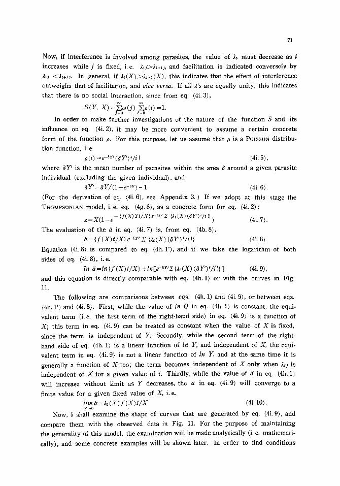
71

Now, if in terference is involved among parasites, the value of ~l~ mus t decrease as i

increases while j is fixed, i.e. 2~j~2~+lj, and facilitation is indicated converse ly by

, ~ <,t~+lj. In general, if a~(X)>2~+I(X), this indicates that the effect of in terference

outweighs that of facilitation, and vice versa. If all 2's are equally unity, this indicates

that there is no social interaction, since f rom eq. (4i. 3), c~ co

S ( Y , X)=32,~o(j) ~ o ( i ) = 1 . j = 0 i = 0

In order to m a k e fur ther invest igat ions of the nature of the function S and its

influence on eq. (4i. 2), it m a y be more convenient to a s sume a certain concrete

fo rm of the function 0. For this purpose, let us assume that 0 is a PomsoN distr ibu-

t ion function, i .e.

p (i) : e -~r' (8 Y') ' / i ! (4i. 5),

where 6Y' is the mean number of parasi tes within the area 6 around a given parasi te

individual (excluding the given individual), and

6Y' = 8 Y / ( 1 - e -~r) - 1 (4i. 6).

(For the derivat ion of eq. (4i. 6), see Appendix 3.) If we adopt at this s tage the

THOMPSONIAN model, i .e. eq. (4g. 8), as a concrete fo rm for eq. (4i. 2):

z : X ( 1 - e - {f(X) Yt/X} e -~Y' X (2~ (X) (5II')*/i !} ) (4i. 7).

T h e evaluation of the // in eq. (4i. 7) is, f rom eq. (4b. 8),

d= { f ( X ) t / X } e -at' X {,is(X) (6Y ' ) ' / i !} (4i. 8).

Equation (4i. 8) is compared to eq. (4h. 1'), and if we take the logar i thm of both

sides of eq. (4i. 8), i .e.

In ii =In { f (X) t / X } + ln[e-Sr'X {~, (X) (6 Y') ' / i !} ] (4i. 9),

and this equation is direct ly comparable with eq. (4h. 1) or with the curves in Fig.

11.

The fol lowing are compar isons between eqs. (4h. 1) and (4i. 9), or be tween eqs.

(4h. 1') and (4i. 8). First , while the value of In Q in eq. (4h. 1) is constant, the equi-

valent t e rm (i. e. the first t e rm of the r ight-hand side) in eq. (4i. 9) is a function of

X; this t e rm in eq. (4i. 9) can be t reated as constant when the value of X is fixed,

since the t e rm is independent of Y. Secondly, while the second t e rm of the r ight-

hand side of eq. (4h. 1) is a linear function of In Y, and independent of X, the equi-

valent t e rm in eq. (4i. 9) is not a linear function of In Y, and at the same t ime it is

general ly a function of X too; the t e rm becomes independent of X only when 2,5 is

independent of X for a given value of i. Third ly , while the value of // in eq. (4h. 1)

will increase without l imit as Y decreases, the d in eq. (4i. 9) will converge to a

finite value for a g iven fixed value of X, i .e.

lim ?i =20 (X) f (X) t / X (4i. 10). Y ~ 0

Now, I shall examine the shape of curves that are genera ted by eq. (4i. 9), and

compare them with the observed data in Fig. 11. For the purpose of mainta ining

the general i ty of this model, the examinat ion will be made analytically (i. e. mathemat i -

cally), and some concrete examples will be shown later. In order to find conditions

72

Under which the value of In ~, for a given fixed value of X, is increasing, decreasing,

or remaining constant, the first order partial derivative Oln ii/Oln Y will be calculated

below:

Oln ii . . dY ' ~-Y,~+I (X) (~Y')~ 1 ) (4i. 11) Oln Y= o" ~ d Y - - - - ; ~ Y ' \ ~

L z 2 , ( x ) ~ ~i )

in which the derivative d Y ' / d Y is, f rom eq. (4i. 6):

d Y' /d Y= { (1 - e -~r) -/~ Ye -~r } / (1 - e -st) 2>0.

From the above evaluation of the partial derivative, the following conclusions will be

drawn:

(1). When Y->O, the partial derivative converges to zero, so that the curve is parallel

to the In Y axis at the level of

In i i= ln{ f ( X ) t / X } +ln 20(X)

(see eq. (4i. 10)). ~ o o

(2). When Y is sufficiently small, so that ~ 2i+1 (X) (~Y') ~/i [ and 2E 2i (X) (~Y') ~/i ! i=1 i ~ l

are negligible as compared with ,h(X)and ;o(X) respectively, then

Oln ii/Oln Y ~ - - ~ Y ( d Y ' / d Y ) {2~ ( X ) / 2 o ( X ) - 1 } .

Therefore: (a) if 2~ (X) >20 (X) , i.e. social facilitation, the curve is increasing

as Y increases, but (b) if At (X) <~0 (X), i.e. interference, the curve is decreas-

ing as Y increases.

(3). The condition (2) can be generalized to a situation in which Y is sufficiently c o

small so that, for a certain number, e.g. k, the sums ZA,+,(X) (SY')*/i! and i = k

oa k - 1

Z A~(X) (SY')*/i! are negligible as compared with the sums ~2~+1 (X)(SY')~/i! i = k i=0

k - 1 and 2EA~(X)(6Y')~/i!. Therefore: (a) if the effect of social facilitation out-

i=0

weighs that of interference, for this range of Y, i.e. k - I k - 1 ~. A,+~ (X) (6 Y ' ) ' / i !> ~ At(X) (SY') ' / i [, i=0 i=0

the partial derivative in eq. (4i. 11) is positive, and so the curve is increasing,

but (b) if the effect of interference outweighs that of facilitation, the curve is

decreasing.

(4). When Y becomes sufficiently large, both lower and higher terms in the series

{2,(X)(~Y')~/i!} will become negligible as compared with mid-terms, i .e. for

certain numbers k and k', we have c o k t

2~(X) (~Y')~/i ! ~ ~ At(X) (~Y') ' / i ! i=O i = k

and the same applies to the series {A,+~(X)(~Y')*/i!}. Now it is unlikely that

the degree of social facilitation increases indefinitely as i increases; the effect

of interference must sooner or later become apparent. Hence, beyond a certain

number for i, e. g. k, the inequality A, (X) >Ak+~ (X) will always hold. Under

these circumstances, the partial derivative becomes always negative, and hence

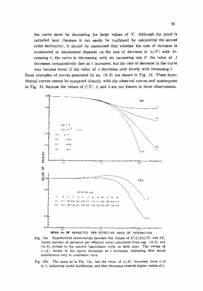
73

the curve must be decreasing for large values of Y. Although the proof is

curtailed here (because it can easily be confirmed by calculating the second

order derivative), it should be mentioned that whether the rate of decrease is

accelerated or decelerated depends on the rate of decrease in 2~(X) with in-

creasing i; the curve is decreasing with an increasing rate if the value of 2

decreases comparatively fast as i increases, but the rate of decrease in the curve

may become lower if the value of 2 decreases only s lowly with increasing i.

Some examples of curves generated by eq. (4i. 9) are shown in Fig. 12. These hypo-

thetical curves cannot be compared directly with the observed curves and scattergram

in Fig. 11, because the values of f ( X ) , t, and ~ are not known in these observations.

tOO

0,50

0,10

0,0. ~

X

: 0

l,f,- 0

=, ~ 1.0C

o~5o

0,IC

Xo(x} = 1.0

e )h(x) = 0,5 I

(1} o= 0

(2 ) = 0,25

13) = 0.50

[z, ) = 0,75

i ' ' ' I I

0,1

( i ~ 1 l

I I I L I I I i | I I I I I I I I I I I

1.0 10,0

t

{1)

(2 )

0 , 2 0 , 5 , B , 0 , 2 , , , 5 \ \,~, 1.00 1,50 0,80 0.50 0.25 0,21 0.18 014 011 0.09 0.08 0.07

1oo , . , 2 o l o o . . . . o.o oJo o: 21; ::: ::; 0,50 030 0.27 0.25 0,23

(1}

. . . . . 0:, . . . . . . . . ,'0 . . . . . . . . ,~0 ' ' MEAN No. OF PARASITES PER EFFECTIVE AREA OF INTERACTION

Fig. 12a. Hypothetical relationships between the values of ii/{f(X)t/X} and 6Y, (mean number of parasites per effective area) calculated from eqs. (4i. 6) and (4i. 8), plotted in the natural logarithmic scale on both axes. The values of 2i (X) shown in the figure decreases as i increases, indicating that social interference only is considered here.

Fig. 12b. The same as in Fig. 12a, but the value of 2 i (X) increases from i = 0 to 1, indicating social facilitation, and then decreases towards higher values of i.

74

However, the similarity in their shapes can be compared, if desired, by parallel

translation of the relative position of the coordinate systems between the observed

and hypothetical relationships, since the curves are drawn on the ln-ln scale. Then,

the shapes of curves (a) and (a') in Fig. l l a are comparable to a certain part of

curve (1) in Fig. 12b. The scattergram (e) in

12a, and so on. A strict comparison will not be

however.

It should be mentioned finally that fitting a

tionships may be justified only for the purpose

Fig. l l b resembles curve (3) in Fig.

at tempted here for the above reason,

straight line to these observed rela-

of showing the declining tendency of

the value of ~ with increasing parasite density. In other words, the only conclusion

that one can draw from such linear regression analysis is restricted to the suggestion

that social interference is involved among parasites. However, there is no justified

basis for adopting the hypothesis that the relationship is linear. Also, the assumption

of the 'quest constant' by HASSELL and VARLEY (1969) (see w 4h) is justified only in

the linear regression analysis of those data in which host density is known to be

constant: the assumption is, however, hardly justified for speculating about the stabili-

ty of host-parasite oscillations in which host density is changing all the time. The

possibility of stable oscillations induced by social interference among parasites is yet

to be demonstrated on a more reasonable basis; until it is, the suggestion by HASSELL

and VARLEY is only a possibility.

Appendix to w 4i. Is the concept of 'area of discovery' useful in studies

of predation and parasitism ?

I t has been shown in this paper that the concept of 'area of discovery', originally

introduced by NICHOLSON (1933), cannot be used as a geometric attribute of the

hunting process, since this simple, but highly hypothetical, concept involves a contra-

diction from the energetics point of view. But the concept has been shifted, as one

way of expressing the hunting efficiency of predators or parasites, and has been widely

used in the literature of population dynamics. The shifted concept is now defined as

d in eq. (4b. 7) for predation and in eq. (4b. 8) for parasitism. The definition, how-

ever, is not a straightforward expression of hunting efficiency, as it is the logarithm

of the reciprocal value of the survival rate, for a specified value of the initial density

of the hunted species per hunter.

My question here is whether this concept of 'area of discovery' is altogether

useful in the study of predation and parasitism. Of course, the concept has played a

significant role in its original context as a species specific constant under a given

condition. But, once the original meaning of this index as a species specific constant

is lost, what does the shifted concept signify ? Is there any particular advantage in

using this index in shifted, and more general, situations ? In order to answer these

questions, the index d will be evaluated in various models reviewed in this paper

and will be compared with the instantaneous hunting function on which each model

75

is based. As the evaluation of t h e / / i s in general different between models for preda-

tion and parasitism, I shall use a symbol //, for predation and i/2 for parasitism, so

that: //1 : 1 x0 In _r X o - - z

i i 2 = l _ l n X X - z "

Also, the expression f(x, Y) will be used as a general form of the instantaneous

hunting function; x should be replaced by X for parasitism.

1. The LOTKA-VOLTERRA model

The definition of //1 does not fit here, since the model takes into account changes

in the densities of both predator and prey populations during the hunting period, t.

In other words, first, the value of Y, defined as a fixed predator density during t,

does not exist, and secondly the value of z is influenced by mortality in the prey

population due to factors other than predation. Under these general circumstances,

the redefined concept of 'area of discovery' just does not exist. If, however, it is as-

sumed as a specific case that mortali ty in the prey population does not occur except

by predation, and that predator density is fixed during t, the model converges to the

NICHOLSON-BAILEY model.

2. The NICHOLSON-BAILEY model

f(x, Y)=ax

//1 =at.

3. HOLLING'S disc model

f(x, Y)=ax/( l+ahx)

//1 : a t - a h z / Y / /2-at/( l+ahX), under the THOMPSONIAN assumption.

4. IVLEV'S model

f(x, Y) = b (1 - e -~') //1 = - (1/Y) In [-1 + (1/axo) In { (1 - e - axo) e - abYt + e- aXo } ]

i iz-bt(1-e-~x)/x , under the THOMPSONIAN assumption.

5. WATT's model

Same as IVLEV'S, but a ~ a y l - ~ .

6. ROYAMA'S model in w 4e

f(x, Y) =a (x) x Yt/{1+ a (x) hx} where a (x) is defined in p. 46, w 4e.

//1: may be evaluated from eq. (4e. 9), but since its analytical solution

with respect to z is difficult, the evaluation will not be at tempted

here.

62 =a (X) t~ {1 +a (X) hX}, under the THOMPSONIAN assumption.

7. THOMPSON'S model

~i2=n/XY,

and if n is evaluated as f (X , Y ) Y t ,

ii2=f(X, Y ) t / X .

So, if f (X , Y ) = a X as in the NICHOLSON-BA[LEY model,

gi 2 - at.

8. The HASSELL-VARLEY model

ii2_O y -,~

or, using my system of notations,

5z =aY1-Bt.

(Note that the THOMPSONIAN assumption is inherent to this model. )

9. ROYAMA'S model in w

52 -e -~y' ~. ~2~(X) (~Y')~/i!} f ( X ) t / X , under the THOMPSONIAN assumption. i-0

(For symbols, see eq. (4i. 8) .)

A comparison between the evaluation of the 52 and the function f (as in the

second equation in 7 above) clearly shows that the 'area of discovery' of parasites

of the indiscriminate type is directly related to the instantaneous hunting efficiency

under the THOMPSONIAN assumption, i.e. that the distribution of parasite eggs fol-

lows a POISSON series. In other words, the shifted concept of 'area of discovery',

under the THOMPSONIAN assumption, still maintains its significance as an index of

the hunting efficiency of the parasites concerned. Such significance, however, is re-

stricted only to the situation in which the THOMPSONIAN assumption holds. If a gener-

alization is made to cover those indiscriminate parasites which do not distribute

eggs after the POISSON fashion, those which discriminate between parasitized and

unparasitized hosts, or predators, the 'area of discovery' is not directly related to the

hunting efficiency (compare, for instance, the 5Vs with corresponding f ' s in the above

list). Furthermore, if the 'area of discovery' is calculated from data in which mortali ty

in either hunting or hunted, or both, species occurs during the hunting period, as is

the case with the LOTKA-VOLTERRA model, the index cannot be calculated. This

suggests that the calculation of the index from the data obtained in the field is theo-

retically difficult, since mortali ty among the hunting species certainly occurs; calcu-

lating the index by using the average density might be attempted, but then it has to

be remembered that the index could not be linearly related to the efficiency.

Thus, the concept of 'area of discovery' loses its significance on general ground,

and there is no particular advantage in using it. What is essential is to find the

method of determining the instantaneous hunting function directly. This problem is,

however, beyond the scope of this paper.

j). HOLLING'S hunger model

In w 3, I showed one method of incorporating the hunger component. The hunger

level there was defined by function H which expressed a partial realization of the

potential maximum performance that each predator can exert in hunting at given

prey and predator densities. HOLLING (1966), in his study of the predation behaviour

77

of Hierodula crassa GIGLIO-TOs., approached the problem from a different direction.

A female mantid, H. crassa, had been deprived of food for various lengths of t ime

before flies (as prey) were offered, and then the weight of flies eaten by the mantid

was measured for each length-class of deprivation time. It was found that the weight

of flies eaten increased as the deprivation time increased (and hence the mantid was

hungrier), gradually leading to a plateau.

The effect of hunger revealed itself not only in the mantid's increased demand

for food to the level of satiation, but also in other components, e.g. the size of the

area of reaction to the prey, speed of reaction, capture success, time spent in pursuing

and in eating prey, and in the digestive pause. The influence of the deprivation time

on each of these components was expressed by separate descriptive equations which

were then synthesized to describe the relationship between the number of prey killed,

the density of prey, and the time involved; the relationship thus obtained was illust-

rated by HOLLING (1966) in his figure 29.

It is not my intention here to review critically every detail of HOLLING'S mathe-

matical treatment, as the study of the effect of hunger is still in its infancy, and also

because I have not had sufficient experience with the problem myself. There are,

however, a few things to be pointed out which HOLLINC seems to have missed.

First, in this study again HOLLING did not recognize the effect of diminishing

returns. It is not certain whether, in the observation that appeared in his figure 29,

the prey density was kept constant during each set of observations. If so, the figure

represents an instantaneous hunting surface equivalent to eq. (3. 18) in which dx/d t

is written simply as n. If, however, the prey density was depleted during the course

of observation, the figure represents a particular one of the overall hunting surfaces

which is specific only to the mantid density used in this particular experiment. In

this case, the density of predators should have been stated (the number of mantids

used might have been just one, but as the fly density was expressed per square cen-

timetre, the mantid density could not be unity). Also, the theoretical curve fitted to

the data in the same figure is in fact an instantaneous rate, and so if the density was

depleted, the comparison is not justifiable.

Secondly, if our aim is to obtain an overall hunting equation, which is no doubt

needed in population dynamics, an appropriate instantaneous hunting equation is

required, the reason for this being explicit in earlier sections of the present paper.

To obtain an instantaneous hunting equation, f rom which the final synthesis is made,

the experimental analysis of the elemental components should have been designed

accordingly. However, the observed relationship, for instance, between the amount of

prey eaten and the deprivation time in HOLLING'S original paper (1966, figures 4 and

5) is not appropriately tailored for the above purpose. This is because the time

involved in consuming a given amount of prey was not explicitly considered by the

author. Suppose the amount eaten up to the state of satiation (see HOLLING'S defini-

tion, 1966 p. 16) was W~ and W2, when the deprivation time was 7", and 2"2, and tl

78

and t2 hours were required to consume WI and Wz, respectively, after the flies were

offered. Then the rates of consumption W~/t~ and W2/t~ could be considered as

instantaneous rates if tl and t2 were not too large. It might be technically difficult to

keep tPs sufficiently small, for otherwise W's could not be measured. If t's are long,

then digestion may take place during those hours, and this must influence the value

of W. Then what is required is the measurement of the relationship between W and

t for various Tts, f rom which the instantaneous rate, d W/dt, may be obtained. And,

of course, it is d W/dt which should be incorporated in the synthesized instantaneous

hunting equation.

Although HOLLING'S approach, which he called an 'experimental component analy-

sis', is no doubt important, some technical difficulties are expected, namely how to

design experiments to meet theoretically required conditions; the example cited above

clearly illustrates these difficulties. This is why I proposed a simpler approach in w 3,

which can tentatively be used for calculating a predator-prey interaction without going

through the details of physiological studies of hunger.

In passing, HULLING tOO used differential equations, which could yield curves

resembling observed ones, without attaching any significance to the equations as the

means of inference. I must again suggest avoiding this unjustifiable operation.

5. DISCUSSION AND CONCLUSIONS

In this section, I shall deal with problems that are more methodological than

technical. Before doing so, however, what was dealt with in w 4 will be summarized

in the following diagram (Fig. 13). It is a flow diagram of reasoning leading to

each model reviewed, and shows the scope that is covered by that model. The dia-

gram is based on my own study and not necessarily identical to what the authors

claimed in their original papers, as their verbal statements were often wrong.

The reasoning starts from (A), a generalized instantaneous hunting equation.

This generalization is obvious from eq. (3. 18), in which H(x, Y, t)f(x) can be written

as f(X, Y, t) if x is fixed at X. From (A) there are two main streams, dealing with

parasitism and predation.

The predation flow is further divided into subflows 1 and 2. Subflow 2 goes

directly to the determination of specific forms of (A) to evaluate n, the number of

prey taken per unit area in t ime interval t when the prey density is kept constant.

All the models after 1955 (except mine) belong to this flow. Since (A) is an instan-

taneous equation, it cannot be used for comparison with observation except for cases

in which reduction in the prey density can be neglected. Also (A) does not give any

means of estimating the final density of the prey or host population at the end of

each generation. Hence, these equations in the category of (A) cannot be used, as

they stand, for the study of prey-predator or host-parasite interaction systems.

Subflow 1, however, incorporates the effects upon the number of prey taken per

unit area (i. e. z) of (a) diminishing returns, (b) changes in the number in the prey

79

population caused by factors other than predation, and (c) changes in the numbers

in the predator population. All the classical models before 1935, and also mine, come

into this flow. In the diagram, (a), (b), and (c) are assumed to be independent of

each other, and under this assumption the simultaneous equations (B) are a priori.

However, if there is any interaction between these effects, the equations are not a

priori and so need experimental confirmation. Also, the use of calculus can be justi-

fied only under the assumption that the pattern of the~ispatial distribution and move-

ments of the animals concerned remain unchanged throughout the time-interval t.

This is perhaps only approximately so, or may be even a very poor approximation as

my first simulation model for predation in w clearly shows, and it requires experi-

mental verification. Until then calculus is only a tentative method.

In the step under the heading 'special cases' in the diagram, the flows diverge

according to the more specific assumptions adopted, and within the scope of each

hypothetical situation (or assumption adopted), all of them are legitimate in that

there is no logical contradiction at this stage. This step is followed by the specification

of the functions involved, under the heading 'specific equations'.

The specific forms of the function f ( X , Y, t) are one of the major concerns in

this study. The meaning of each form was interpreted in the light of the geometric

properties of hunting behaviour under the assumption of random distribution in the

prey population. The assumption of random distribution is legitimate in a theoretical

study like this, as the first step towards more general, irregular distribution patterns

in future studies (the problem will be discussed elsewhere). Some other assumptions

appearing in certain specific forms in WATT (1959), NICHOLSON-BAILEY (1935), LOTKA-

VOLTERRA (1925-1926), and GAUSE (1934) are not legitimate: in the WATT equation,

as well as in HASSELL and VARLEY, rl-,~ as a measure of the degree of social inter-

action is contradictory to the premise that a predator has a limited capacity to attack

its prey; in the NICHOLSON-BAILEY equation, f ( x ) as a linear function of x is a priori

impossible; in the LOTKA-VOLTERRA equations, the same criticism as in the NICHOLSON-

BAILEY applies, and also the assumption of a constant r ' is theoretically incorrect;

finally, in GAUSE'S equation, his suggestion concerning g~(x)-- f (x)y (GAusE 1934,

formula (25), p. 57) is not comprehensible.

The evaluation of z (the reduction of the prey density during time-interval t in

a system with discrete generations) is possible only through the reasoning of subflow

1. Such an evaluation was made in the original literature only by NICHOLSON and

BAILEY. All of the three recent models (i.e. IVLEV, HOLLING, and WATT) were

concerned only with the evaluation of n, and LOTKA and VOLTERRA gave only one

special solution for a system with continuous generations. Therefore, tho~e evaluations

in the diagram were made in the present study (w 4). It should also be mentioned

here that the evaluation of z made in this study, except for the LOTKA-VOLTERRA

equations, assumed that both functions gl and g2 were zero as in the NICHOLSON-

BAILEY equation, but this is only possible in an idealized, experimental set-up. The

80 �84

assumption, however, plays a legitimate role in the process of inferences as discussed

in w 2. If the assumption does not hold, the functions gl and gz have to be determined

experimentally, as there seems no method presently available to deduce specific

forms for these functions by analogy. But this problem is not relevant to the present

study of hunting behaviour.

GAUSE'S model is inadequate, because the logistic law was taken into account

only in gl and not in g2. Also, f is not specified. It is pointed out here, however,

that GAUSE'S equation is applied specifically to a system with continuous generations,

since the introduction of a logistic function as a specific form for g~ positively ex-

cludes the case of discrete generations.

It is clearly shown in this comparative study that it is LOTKA and VOLTERRA,

the pioneers in the theoretical study of the prey-predator interaction system, whose

thought and insight covered the widest scope, and who laid the foundation for the

formalization of the system, although their specific forms were unsatisfactory. All

other later models covered only a fraction of the basic structure of the system. Yet,

surprisingly, none of the later authors appeared to be aware of this fact. Thus,

NICHOLSON and BAILEY proposed their model as an alternative to the LOTKA-VOLTERRA

one without noticing that the scope of their model had already been potentially covered

by the earlier model. In other words, while LOTKA and VOLTERRA gave one solution

to a system with continuous generations, the NICHOLSON-BAILEY competition equation

is nothing more than another solution of the LOTKA-VOLTERRA equations in a system

with discrete generations. The at tempts by HOLLING, IVLEV, and WATT were con-

cerned only with the improvement of the specific form of function f , and completely

neglected the reasoning along subflow 1 in Fig. 13, and thus these authors failed to

separate n from z. WATT'S proposal of his equation even involves a contradiction;

the proposal can hardly be called an improvement. Yet, the claims by these recent

authors that their models were more realistic than the classical ones have been ac-

cepted by many ecologists in this field. These facts are an indication of the lack of

rigorousness in the attitude of ecologists, and this will be considered below.

First, some concepts and terminology used in this field of ecology are too loose;

thus confusion occurs in communication between ecologists or even within the mind

of a single person. For example, WATT (1962) stated that the classical models failed

because the reasoning started f rom 'a priori assumption' and was purely deductive,

and thus he proposed (WATT 1959) what he called a 'deductive-inductive method'.

This criticism of the classical models and the proposal of the alternative are not

convincing for the following reasons.

First, the premise in the classical models as appeared in specific form, e.g. f (x )

=ax, is not a priori. Strictly speaking, the phrase a priori means that which is

"marked by being knowable by reasoning f rom what is considered self-evident and

therefore without appeal to the particular facts of evidence" (WEBSTER'S 3 rd Interna-

t ional Dictionary 1968), f rom which is derived secondarily that which is ' intuitive' or

81

'without experience'. If one uses the phrase to mean just ' intuitive or without expe-

rience' completely emancipated f rom the original meaning, one might include any as-

sumption set forth without confirmation by observation. Then, the expression 'a priori

assumption' is tautological, since an 'assumption' is a premise adopted before a thing

is known. Although the premise in the classical models was set forth without support

from factual evidence, it is not a priori. On the contrary, the premise is a priori

impossible as it violates the second law of thermodynamics. If any reasoning starts

from an assumption which is a priori impossible, the conclusion drawn deductively

is bound to be contradictory upon comparison with a fact. (This is the case with c22

under C2 in w Thus, it is to be expected that the specific form of the classical

models would fail to describe real events satisfactorily. This, however, does not

entirely invalidate the classical models, as will be shown later.

The second point is concerned with deductive and inductive methods of inference.

Today everyone knows, as WALKER (1963) pointed out (see w 2), that deduction

does not produce more than has been involved in the premise, and therefore this

method of inference alone will not contribute to our knowledge of natural order. I t

is impossible to believe that mathematicians like LOTKA and VOLTERRA did not know

this rule: rather, they must have had a firm reason to present their models as deduc-

tive ones. We know, as FRANCIS BACON himself had long ago pointed out, that a

simple induction, i.e. a mere enumeration of facts, is no better, and even 'childish',

and that a new concept would be formed only by what BACON called 'gradual induc-

tion', i.e. a gradual passage from concrete facts to broader and broader generaliza-

tions (DucASSE 1960). The process of gradual induction, however, does not exclude

a phase which is deductive, e.g. once a certain assumption is made, perhaps by

induction, a conclusion can be drawn only by reasoning, and then this conclusion is

compared with observation. This is very similar to what I described in w 2. My

interpretation of the LOTKA-VoLTERRA method is that they were showing what such

deductive phases of reasoning could be like. Tha t is, what they have shown is a

model of deductive reasoning which is conveniently separated from the entire process

of inference.

I t was rather unfortunate that the premise in the classical models was in fact

biologically absurd (IVLEV 1961) and did not appeal to ecologists. However, for a

mathematician who tries to show the basic structure and the method of analysis (to

form a hypothesis), the adoption of such specific forms might have been merely

trivial and only tentative since it can be changed readily if desired; but the principle

of the mathematical method remains uninfluenced. This attitude is very clear in

LOTKA'S work. I t is unfortunate that ecologists became too much concerned with

such a casual premise and failed to see the more fundamental aspect of the idea.

This point is clearly illustrated in the three recent model builders, as reviewed above,

who failed to distinguish n from z. This failure to understand the classical model

is not only seen in these authors but also in others (e. g. ANDREWARTHA and BIRCH

82

1954; MILNE 1957) who thought that the premise and the structure of the classical

models were far too simple to be realistic. It should be pointed out, however, that

those who proposed what was claimed to be more realistic, taking so many conceiv-

able factors into account, have never been able to formalize the ideas that they stated

only verbally, or have not even tried to do so. From such verbal statements, one

cannot draw a quantitatively expressed conclusion that can be compared with ob-

served quantities for testing.

Now it is clear that the criticism of the classical models was due to insufficient

understanding of the nature of inferences. As pointed out in w 4f, although WATT

claimed that the assumption of the coefficient A as it appeared in eq. (4f. 5) was

based on an empirical fact, it was in fact an illusion, since the assumption proved to

be nothing but dogmatic and even impossible a priori. Obviously, the author did not

test his hypothesis (i, e. eq. (4f. 5)) by any means and this positively violates, con-

t rary to what was claimed, the code of rules for inferences by induction. The same

criticism applies to the HASSELL-VARLEY model in w 4h.

The above discussion suggests that the stage we are in is still very primitive,

with an evident lack of rigor in methodology. This, however, may well be because

the nature of the objects we are studying have influenced the development of ideas

in this field. My point may be illustrated by contrast with the development of the

physical sciences.

In physics, some properties of certain objects were, very fortunately, describable

deterministically (sensu BORN 1964--predictable without the causal relationships being

known; a timeless and spaceless link between the events, e.g. a railway time-table).

The arithmetic prediction of the stars ' motion by the Babylonians or, more recently,

KEPLER'S Law, are perhaps typical examples. As modern physicists went into the

more minute details of atoms, and as the required measurements became finer and

finer, they eventually reached a stage where the classical method of induction was no

longer applicable. A positive barrier was encountered when HEISENBERG enunciated

his Uncertainty Principle in 1927; this predicts that some physical attributes of the

object being measured are influenced by interaction between the object and the meas-

uring system. However, before this stage was reached, there were enough examples

of success in macrophysics, i.e. in NEWTONIAN physics, which encouraged the phys-

icists to explore thoroughly the method of induction.

In the field of population dynamics, however, difficulties similar to those that

modern physics is currently facing have been a major problem from the beginning.

Some may be only technical difficulties in obtaining accurate measurements. For

example, the concept of the handling time (h), originally suggested by HOLLING

(1956), was found to be highly idealized in my study of the great tit, Parus major

L. (ROYAMA 1970). I tried to t ime the tit as it searched for food and as it handled

each item. The information was used to calculate a theoretical value for the amount

of food that the tit could collect per day using HOLLING'S disc equation (for the

83

justification of its use, see ROYAMA 1970). It was found that, for an intuitively rea-

sonable magnitude for the factor a, the calculated value for h was ridiculously high.

When the factor a was so adjusted as to obtain a more reasonable value for h, then

such values of a were inexplicably low. My conclusion was therefore that the estima-

tion of h by observation was far lower than it actually was. This is perhaps because

what was recorded as searching time must have contained a high proportion that was

spent upon various activities other than pure searching, e.g. watching for enemies.

These activities must have occupied such short intervals that they were hardly sepa-

rable by direct observation.

Beside such difficulties in measuring each activity separately and accurately, there

are more profound ones which may not be solved technically. The first is the time

factor. In order to take a sufficiently reliable measurement, say, of the fluctuation in

numbers of an animal species from year to year, the life span of a single ecologist

may not be sufficiently long: perhaps he can study only some twenty generations of

a univoltine species. From a mere accumulation of sampling data, he can draw

conclusions by guessing, not by induction. The second difficulty lies in differences

between natural and experimental situations. The development of comparative ethology

in the past decade shows that the behaviour of animals has so evolved that its biologi-

cal goal is attained by responding appropriately to a chain of stimuli provided in

the animals' natural environment (see e.g. TINBERGEN 1951; for more recent develop-

ment see HINDE 1966). We cannot be certain on the one hand, however, if some of

the necessary stimuli are lacking in an experimental set-up in which the animals

concerned may not behave in an intelligible manner. But, on the other hand, we may

not be able to know, without experimental studies, what stimuli are involved in the

animals' normal environment where evolution has taken place. Then we will not be

certain whether we can establish a fact from which to follow the formula of induction

laid out by the classical physics, or rather if a fact at hand is a meaningful one that

can be used to start the gradual process of induction.

These arguments may be metaphysical problems, but are sufficient to show that

the primitive stage we are in at the moment, as compared with physical sciences, is

perhaps due to the above-mentioned difficulties, which prevented us consciously or

subconsciously from developing the method of inference by induction, starting from

an elemental stage where a deterministic prediction would not have been hard to make.

For the time being, ecology will perhaps remain largely descriptive, even if we

cannot expect to develop a deterministic law governing the hunting behaviour of

animals directly from such enumerations. A theoretical study by models, i.e. infer-

ence by analogy, will not replace the tedious process of enumeration, but it will at

least partially help in the interpretation of observed facts. The method will be useful,

however, only provided that the models are appropriately constructed and used. The

idea is perhaps the same as that suggested by OPPENHEIMER (1956) to a group of

psychologists as 'pluralism' in the method.

84

What is required at the present stage is to make use of the formalism of mathe-

matics to a thorough extent in the quest of certitude. Some ecologists might suggest

that the complexity of natural order almost prohibits this formalism. But this amounts

to giving up the quest for certitude, because, if mathematics cannot handle the com-

plexity, it would be even more difficult for the verbal method of inference to cope

with the problem, and we do not have a better alternative, at least at the present

stage of the development in population dynamics.

6. SUMMARY

1. This is a critical study of major existing models for predation and parasitism,

and its aim is to evaluate the roles played, or those not played, by these models in

helping our insight into the relationships underlying prey-predator and host-parasite

interaction systems.

2. The concept of a model, and the role it plays in the process of reasoning that

leads eventually to understanding of the system, is considered first in general terms.

I t is pointed out that a model is a means through which a hypothesis is formed;

the model is an analogy to the thing to be understood, constructed from already

known concepts.

3. The basic structure of predation and parasitism are then presented in terms of

mathematical equations of general forms. This is to help readers to understand the

examination of existing models which follows in the subsequent sections. Two differ-

ent sets of inferences are discussed, the one leading to a model for predation and

the other to a model for parasitism. The role played by a differential equation as a

means of deduction is explained.

4. Models proposed by LOTKA, VOLTERRA, NICHOLSON and BAILEY, HOLLING,

IVLEV, GAUSE, ROYAMA, WATT, THOMPSON, STOY, and HASSELL and VARLEY are

critically examined, with particular attention to their logical structures rather than

to their ability to generate a theoretical trend that superficially fits an observed one.

The logical structures of these models are summarized in the form of diagrams in

w 5. The critical study is developed by means of analogies to various geometric

models, which clearly show some misconceptions involved in each model reviewed.

It also shows that the logical structure in the classical models (those proposed before

1935) are sound, but the assumptions involved are often inadequate to describe an

actual biological system; on the other hand, recent models (proposed after 1955) either

involve contradiction in logic or are much too often erroneously applied to the analysis

of actual predation and parasitism. It is pointed out that the mere fitting of curves

to data can neither establish a particular mechanism nor provide verification of the

model concerned.

5. Finally, the types of inferences, which can or cannot help us in understanding

the processes of predation and parasitism, are considered by comparison to similar

problems in the development of physical sciences. In ecology, inference by induction,

85

which has been and Still is to a large ex ten t the major scientific method, has inherent ly

many of the s a m e problems as modern physics, such as HEISENBERG'S Uncer ta in ty

Principle. Perhaps cer ta in types of difficulty that are encountered by the observat ional

method can be overcome, if not entirely, wi th the aid of inferences by analogy, and

it is in inferences where the model plays its role.

ACKNOWLEDGEMENTS: I am grateful to the following people for their very constructive com-

ments and suggestions which led to much greater clarity in my presentation: Drs. R.F. MORRIS,

G.L. BASKERVILLE and M.M. NEILSON (Canadian Forestry Service, Fredericton), M.E. SOLOMON

(University of Bristol), and Y. IT6 (National Institute of Agricultural Sciences, Tokyo). Professor

S. TANAKA'S (Ocean Research Institute, University of Tokyo) comments on my mathematical treat-

ments helped to minimize erroneous arguments.

REPERENCES

ANDREWARTItA , H.G. and L.C. BIRcH (1954) The distribution and abundance of animals. Univ.

Chicago Press, Chicago.

BLiss, C.I. and R. A. FISHER (1953) Fitting the negative binomial distribution to biological data

and note on the efficient fitting of the negative binomial. Biometrics 9 : 179-200.

BORN, M. (1964) Natural philosophy of cause and chance. Dover, New York.

BURNETT, T. (1956) Effects of natural temperatures on oviposition of various numbers of an insect

parasite (Hymenoptera, Chalcidoidae, Tenthredinidae). Ann. Ent. Soc. Amer. 49:55-59.

BURNETT, T. (1958) Effect of host distribution on the reproduction of Encarsia formosa GAHAN

(Hymenoptera : Chalcidoidae). Can. Ent. 90 : 179-191.

BURNSIDE, W. (1928) Theory of probability (1959 ed.). Dover, New York.

CHAeMA~, R.N. (1931) Animal ecology. McGraw-Hill, New York & London.

CLAaK, P.J. (1956) Grouping in spatial distributions. Science 123 : 373-374.

CLARK, P.J. and F. C. EVANS (1954) Distance to nearest neighbor as a measure of spatial relation-

ship in populations. Ecology 35 : 445-453.

DRAKE, S. (1957) Discoveries and opinions of GALILEO. Doubleday, New York.

DUCASSE, C.J. (1960) FRANCIS BACON'S philosophy of science. Chapter 3 in "Theories of scientific

method : Renaissance through the nineteenth century". Univ. Washington Press, Seattle.

ELTON, C. (1935) Review of A. J. LOTKA (1934). ~ Anita. Ecol. 4 : 148-149.

GAMOW, G. (1962) Gravity. Doubleday, New York.

GAuss, G.F. (1934) The struggle for existence. Williams & Wilkins, Baltimore.

GRIFFITnS, K.J. and C.S. HoLLInG (1969) A competition submodel for parasites and predators.

Can. Ent. 101 : 785-818.

HASSELL, M.P. and G. C. VARLEY (1969) New inductive population model for insect parasites and

its bearing on biological control. Nature 223 : 1133-1137.

HAYNES, O.L. and P. SIsojEvtc (1966) Predatory behavior of Philodromus rufus WALCKENAER (Ara-

neae : Thomisidae). Can. Ent. 98 : 113-133.

HINDS, R.A. (1966) Animal Behavior. McGraw-Hill, New York.

HOLLIN6, C.S. (1959a) The components of predation as revealed by a study of small mammal

predation of the European pine sawfly. Can. Ent. 91 : 293-320.

HOLLINC, C.S. (1959b) Some characteristics of simple types of predation and parasitism. Can. Ent. 91 : 385-398.

86

HOLLING, C.S. (1961) Principles of insect predation. Ann. Rev. Ent. 6 : 163-182.

HOLLING, C.S. (1966) The functional response of inver tebra te predators to prey density. Mere.

Ent. Soe. Can. 48:3-86.

HUFFAKER, C.B. and C. E. KENNETT (1969) Some aspects of assessing efficiency of na tura l enemies.

Can. Ent. 101 �9 425-447.

ITb, Y. (1963) DSbutsu Seitai-gaku Ny~mon (Introduction to animal ecology]. Kokin-shoin, Tokyo.

IVLF.V, V.S. (1955) Experimental ecology of the feeding of fishes (English t ranslat ion by D. SCOTT

1961). Yale Univ. Press, New Haven.

LAING, J. (1937) Host finding by insect parasites. I. Observations on the finding of hosts by

Alysia manducator, Mormoneilla vitripennis, and Trichogramma evanescens. J. Anita. Ecol.

6 : 298-317.

LOTKA, A.J. (1925) Elements of physical biology. Williams & Wilkins, Baltimore.

MILLSR, C.A. (1960) The interact ion of the spruce budworm, Choristoneura fumiferana (CLsM.),

and the parasi te Glypta fumiferana (VIEs.). Can. Ent. 92 : 839-850.

MILNE, A. (1957) Theories of na tura l control of insect populations. Cold Spring Harbor Syrup.

Quant. Biol. 22 : 253-267.

MORRIS, R.F. (1963) The effect of predator age and prey defence on the functional response of

Podisus maculiventris SAY to the density of Hyphantria cunea DRURY. Can. Ent. 95 : 1009-1020.

MORISXTA, M. (1954) Est imat ion of population density by spacing method. Mere. Fac. Sci. Kyushu

Univ. E 1 : 187-197.

NICHOLSOS, A.J. (1933) The balance of animal populations. J. Anim. Ecol. 2 �9 132-178.

NmaoLsor~, A.J. and V. A. BAILEY (1935) The balance of animal populations. Par t 1. Proc. Zool.

Soc. London 1935, Pa r t 3 : 551-598.

OeeENamMsa, R. (1956) Analogy in science. Amer. Psychol. 11 : 127-135.

PEARL, R. (1927) The growth of populations. Quart. Rev. Biol. 2 : 532-548.

POINCARL H. (1952) Science and hypothesis (English ed.). Dover, New York.

PogvA, G. (1955) Mathematics and plausible reasoning. Vol. 2. Patterns of plausible inference.

Princeton Univ. Press, Princeton.

ROYAMA, T. (1966) Mathemat ical models of predatory behaviour in population dynamics. (In

Japanese.) Biol. Sci., Tokyo, 18 : 97-105.

ROYAMA, T. (1969) A model for the global var ia t ion of clutch size in birds. Oikos 20 : 562-567.

RO~rAMA, T. (1970) Factors governing the hunt ing behaviour and selection of food by the great

tit, Parus major L. ]. Anita. Ecol. 39 : 619-668.

RUSSELL, E.M. (1961) Soil conditions and plant growth (9th ed.) Longmans, Norwich.

SCHON, D.A. (1967) Invention and the evolution of ideas. Butler & Tanner , Frome & London.

SMITH, H.S. (1939) Insect populations in relations to biological control. Ecol Monogr. 9 : 311-320.

SIMMONDS, F.J . (1943) Occurrence of superparasi t ism in Nemeritis canescens. Rev. Can. Biol.

2 : 15-40.

STov, R.H. (1932) Appendix to G. SALT (1932) [Superparas i t i sm by Collyria calcitrator GRAV.]

Bull. Ent. Res. 23 : 215-216.

THOMPSON, W.R. (1924) La th6orie math6mat ique de Faction des parasi tes entomophages et le

facteur du hassard. Ann. Fac. Sci. Marseille 2".69-89.

THOMeSON, W.R. (1939) Biological control and the theories of the interact ion of populations.

Parasitology 31 : 299-388.

87

TINBERGEN, L. and H. KLOMP (1960) The na tura l control of insects in pinewoods. II. Conditions

for damping of Nicholson oscillations in parasite-host systems. Arch. ne~rl. 7.ooi. 13 : 344-379.

TINBERGEN, N. (1951) The study of instinct. Clarendon Press, Oxford.

TORII, T. (1956) Konchfe-Shftdan no Suikei-h5 [Statistical analysis of insect populations]. Chapter 7

in "Seitai-gaku Gaisetsu" [Outline of ecology,, (ed. by N. YAGI and K. NOMURA). Yoken-do,

Tokyo.

TOULMIN, S. (1961) Foresight and understanding. Harper (Torchbook ed. 1963), New York & Evanston.

ULLY~TT, G.C. (1947) Mortal i ty factors in populations of Plutella maculipennis CURTIS (Tineidae :

Lep.), and the i r relat ion to the problem of control. Ent. Metal, Dep. Agr. Forest., Union of

South Africa 2 (part 6) : pp. 202.

ULLY~TT, G.C. (1949a) Distr ibut ion of progeny by Chelonus texanus CRESS. (Hymenoptera : Brac-

onidae). Can. lent. 81:25-44.

ULLYETT, G.C. (1949b) Distr ibution of progeny by Cryptus inornattus PRATT (Hymenoptera : Ichneu-

monidae). Can. Ent. 81:285-299.

VBRnURST, P.E. (1838) Notice sur la loi que la population suit dans son accroissement. Corresp.

Math. Phys. 10 : 113-121.

VOLT~RRA, V. (1926) Variazioni e fluttuazioni del numero d'individui in specie animali conviventi.

Mere. R. Accad. Naz. dei Lincei, Ser. VI, Vol. 2 [English t ransla t ion in CHAeMAr~ 1931].

WALKER, M. (1963) The nature of scientific thought. Prentice-Hall, New Jersey.

WATT, K. E.F. (1959) A mathemat ica l model for the effect of densities of at tacked and a t tacking

species on the number attacked. Can. Ent. 91 : 129-144.

WATT, K. E.F. (1961) Mathemat ical models for use in insect pest control. Can. Ent. Suppl.

1 9 : 1-62.

WATT, K .E .F . (1962) Use of mathemat ics in population ecology. Ann. Rev. Ent. 7:243-260.

WATT, K. E.F. (1968) Ecology and resource management. McGraw-Hill, New York.

WILLIAMS, C.B. (1964) Patterns in the balance of nature and related problems in quantitative

ecology. Academic Press, London & New York.

8 8 �84

Appendix 1. The proof of L I = I / 2 R X :

Suppose particles of kind P are dis t r ibuted at r andom with density X over a two-dimensional

plane of sufficiently large area. Let l be the distance between Q's s ta r t ing point A and the periph-

ery of the circle of radius R around P tha t Q first encountered from outside the circle when

moving in an a rb i t ra r i ly determined direction. Suppose tha t l comprises very small sections of

length ,~l, and t ha t l~ is defined by izll ( i=1 , 2 . . . . . c~o). Let ~7l be the probabil i ty tha t a t least

one part icle of kind P falls within, and only within, a locus (li, l i+dl). Then the average distance

t h a t Q travels f rom outside to encounter the per iphery of the first, i .e. L~, is oo

Lt=lim ~2 IpT~ (i). d l~O i = l

Now, ~2~ is the product of the following probabil i t ies:

(1) probabil i ty tha t a t least one part icle of kind P is found within area 2R(li+zff), which for

the assumption of the Po~ssos distr ibut ion is, for j = l , 2 . . . . . cr

~,, [ {2R(l~+dl) X} J/j !] e -2R(I,+aI)X, j - 1

(2) probabil i ty tha t all of these j part icles within area 2R(li+dl) are found within locus (li, li

+dl), i.e. {2RJ1/2R (l~ +all) } ~.

Thus,

~ = ~ [ (2R (li + AI) X} J/j !]e-2R(h + ~l)X {2Rdl/2R (li + Jl) }

= ~, { (2RJIX) J/j !} e 2 R J I X - 2RI~X

j = l

- 2 R d l X - 2 R l i X = ( 1 - e ) e

Since, by a theorem in the theory of limit,

lira (1 - e - 2R~IX) ~all = 2 RX, J l ~ 0

and so, by wri t ing l~ simply as l, we have

lira ~7~ = 2RXe- 2RIX dl. 6l ~ 0

Hence, f rom eq. (i),

L~=2RX f : Ie -2RlX dl

=I/2RX.

Appendix 2. The proof of L 2 = { O ( V ' ~ X R ) / 1 / X - R e -TrR2X } / ( 1 - e -~rR~X )

on a two dimensional plane

Suppose tha t the radius R consists of a number of very small sections of length dr, and tha t

ri is defined as idr( i=l , 2 . . . . . oo). Let tti be the probabil i ty of at least one point of A's fall ing

within, and only within, a locus (ri, ri+dr). Then the average distance between the centre of a

circle of radius R and the neares t A within the circle, i.e. L2, is oo co

Lz=limar~o { i=5-2'1 r~pd / { ~lt~}~ (ii).

Now, pi is the product of the following probabili t ies:

89

(1)

assumption of a PoxssoN distribution,

~E [ {z (r, + J r ) 'Aq s~ j!] e - ~'(' '+ dr)2X , j ~ l

(2) probability that all of these j points fall within a locus (ri, r i + d r ) , i.e.

[ {z (r~ +dr ) 2_ r, ri~}/~r (ri +dr ) 2],,.

With a similar calculation as for 7] in Appendix 1, we have

l . - wr~.X ~m ta~=2~rXe dr. d r--*O

Thus,

Similarly,

probability that at least one point of A's falls w i th in radius r i + d r ; this is, under the

co PR - *rr2X lira i= a~lFi=|o 2r, r X e dr

J r--~0 '=

= l _ e - ~ r R ~ X (iii).

oo PR ~ -wrO-X lira ]E r q 2 ~ = l 2.'rr X e dr

zIr~O i=1 dO

and integrating by parts,

fR2~ , r , e - , r rO~X, [ 'R -wr~ ar=Jo e ' d r - R e - ' R ~ ' x (iv).

Let O(t) be the normal probability function, i.e.

1 t - t 2 / 2 $(t) = . 7 , - - f e dt,

V~Tr JO

and setting t equal to l / 2 z X r , the integral in the right-hand side of eq. (iv) will be writ ten as

�9 ( 1 / ~ R ) / V ' X . Thus, from eqs. (ii), (iii), and (iv) and using symbol ~, we have

L.=[, )

Appendix 3. The proof of eq. (4i. 6)

Let Y be the density of particles distributed at random over an area A, each one of the

particles having a circle of area 6 around it. Then the density of the particles, Y", within the

total area covered with these circles, i.e. A', is

Y " - = - A Y / A '

Suppose that a large number of points, i.e. U, with circles of, also, area ~ are placed to

cover the whole area of A independently of the distribution of the particles. Then, the number

U' of these points that include at least one of the particles will he, on the assumption of the

Poissos distribution,

U ' = U ( 1 - e -~r) (vi),

and the proportion U / U ~ must be equal to the proportion A / A ' . Thus from eqs. (v and vi), we

find

Y " = Y / ( 1 - e - ~ Y ) .

Thus a circle of area c~ around each particle contains on the average 6Y~P number of parti-

cles. However, since ~Y~ is, as defined in w 4i, the mean number of particles in each circle less

the one at the centre, we have

6 Y ' = 6 Y " - - I

= ~ Y / ( 1 - e -~r) - 1 .

90

Appendix 4. List of symbols

The following symbols with the same meaning appear in more than two sections and in the

flow diagram of Fig. 13. Sections indicated in the parentheses are the places where definitions

are given. Symbols used in one section only, or those defined each time they appear, are not

listed.

Variables :

x (w Prey or host density.

X ( / / ) Fixed prey or host density during t. (For t see below. )

x0(H) Initial prey density when /-=-0.

y (H) Predator or parasite density.

Y ( / t ) Fixed predator or parasite density during t.

t ( t t) Interval of a hunting period.

(I t) Number of prey taken, or number of parasite eggs laid, per unit area, when the density

of the hunted species is fixed during t.

z ( t t) Number of prey taken, or number of hosts parasitized, per unit area during t , when

the density of the hunted species is not replenished.

L(w 4c) Time spent in searching only.

:Functional symbols :

f (w 3) Instantaneous hunting function.

F ( tt ) Overall hunting function.

gl(w 4a) Function characterizing the instantaneous rate of increase (or decrease) of prey popula-

tion in the abscense of predators.

g , (M) Characterizing the instantaneous rate of increase (or decrease) of predator population

in the presence of food species.

S(w Characterizing the degree of social interaction (interference or facilitation) among

predators or parasites by which the f changes.

H ( ~t ) Characterizing the partial realization of the potential performance in hunting in accor-

dance with the degree of hunger or satiation.

( t t) Probability of a host receiving no parasite egg.

:Factors independent of the variables listed above :

a (w 4b) Effective area of recognition.

b (w 4d) Positive proportionality factor.

c (zt) Positive proportionality factor.

/~ (w 4f) Coefficient of social interaction. (See also w 4h. )

r(w 4a) Coefficient of increase in prey population in the absense of predators.

r t ( / / ) Coefficient of decrease in predator population in the absense of food species.

a ' ( # ) Coefficient of increase in predator population due to feeding.

h (w 4c) Time spent in handling an individual prey or host.

M(w 4g) Size of hunting area.

Other parameters :

~(w 4b) 'Area of discovery' defined as in eqs. (4b. 9) and (4b. 10).

k (w 4g) Factor characterizing the degree of aggregation in the negative binomial distribution.

(The symbol k used in w w 4c and d stands for the frequency of tapping fingers or that

of tossing rings. )

91

4. LOTKA, VOLTERRA, NICHOLSON ~ BAILEY, HOLLING, IVLEV, GAUSE, ~JJ, WATT, THOMPSON, STOY,

~ , ~ ~ ' ~ : ~ i ~ ~ . l : l ; ~ b ~ ' ~ : ~ 6 ~ b t : P__ ~ 8 , ~ A . ~ ~ ~, ~ / ~ 6 ~ o ~