Embed Size (px)
Citation preview
A COMPARATIVE STUDY OF FIVEALGORITHMS FOR PROCESSING
ULTRASONIC ARC MAPS
a thesis
submitted to the department of electrical and
electronics engineering
and the institute of engineering and science
of bilkent university
in partial fulfillment of the requirements
for the degree of
master of science
By
Arda Kurt
August 2005

I certify that I have read this thesis and that in my opinion it is fully adequate,
in scope and in quality, as a thesis for the degree of Master of Science.
Prof. Dr. Billur Barshan(Supervisor)
I certify that I have read this thesis and that in my opinion it is fully adequate,
in scope and in quality, as a thesis for the degree of Master of Science.
Assoc. Prof. Dr. Orhan Arıkan
I certify that I have read this thesis and that in my opinion it is fully adequate,
in scope and in quality, as a thesis for the degree of Master of Science.
Asst. Prof. Dr. H. Murat Karamuftuoglu
Approved for the Institute of Engineering and Science:
Prof. Dr. Mehmet BarayDirector of the Institute Engineering and Science
ii
ABSTRACT
A COMPARATIVE STUDY OF FIVE ALGORITHMSFOR PROCESSING ULTRASONIC ARC MAPS
Arda Kurt
M.S. in Electrical and Electronics Engineering
Supervisor: Prof. Dr. Billur Barshan
August 2005
In this work, one newly proposed and four existing algorithms for processing ul-
trasonic arc maps are compared for map-building purposes. These algorithms are
the directional maximum, Bayesian update, morphological processing, voting and
thresholding, and arc-transversal median algorithm. The newly proposed method
(directional maximum) has a basic consideration of the general direction of the
mapped surface. Through the processing of arc maps, each method aims at over-
coming the intrinsic angular uncertainty of ultrasonic sensors in map building, as
well as eliminating noise and cross-talk related misreadings. The algorithms are im-
plemented in computer simulations with two distinct motion-planning schemes for
ground coverage, wall following and Voronoi diagram tracing. As success criteria of
the methods, mean absolute difference with the actual map/profile, fill ratio, and
computational cost in terms of CPU time are utilized. The directional maximum
method performed superior to the existing algorithms in mean absolute error, was
satisfactory in fill ratio and performed second best in processing times. The results
indicate various trade-offs in the choice of algorithms for arc-map processing.
Keywords: Ultrasonic sensors, map building, arc maps, Bayesian update scheme,
morphological processing, voting and thresholding, arc-transversal median algo-
rithm, wall following, Voronoi diagram, motion planning, mobile robots.
iii
OZET
ULTRASONIK ARK HARITASI ISLEMEYE DAYALI BES
YONTEMIN KARSILASTIRMALI INCELEMESI
Arda Kurt
Elektrik Elektronik Muhendisligi, Yuksek Lisans
Tez Yoneticisi: Prof. Dr. Billur Barshan
Agustos 2005
Bu calısmada, biri yeni gelistirilmis, dordu ise onceden varolan, ultrasonik ark
haritası isleyerek harita cıkarımına yonelik bes yontem karsılastırılmıstır. Bu
yontemler sırasıyla yonlu maksimum, Bayesian guncelleme, morfolojik isleme, oy-
lama ve esikleme, ve ark-dogrultusal medyan yontemleridir. Yeni gelistirilen yontem
(yonlu maksimum), haritalanan yuzeyin genel dogrultusuna dair temel bir bilgiyi
isleme dahil etmektedir. Tum yontemler ark haritaları isleme yoluyla ultrasonik
algılayıcılara ozgu acısal belirsizligin, sinyal gurultusunun ve capraz-konusmanın
haritalamaya olumsuz etkilerini ortadan kaldırmayı hedeflemektedir. Karsılastırma
amaclı bilgisayar benzetimlerinde alan kapsamaya yonelik olarak duvar takibi ve
Voronoi grafigi cizimi taramaya dayalı iki degisik hareket-planlama yontemi kul-
lanılmıstır. Basarım olcutu olarak cıkarılan haritanın gercek profil ile arasındaki or-
talama mutlak fark, gercek haritanın ne oranda cıkarılabildigine dair doluluk oranı ve
islemin bilgisayar ortamında aldıgı sure kullanılmıstır. Yeni one surulen yontem olan
yonlu maksimum ortalama mutlak hata alanında diger yontemlerden daha yuksek
bir basarı sergilemis, doluluk oranında basarılı olmus, hesaplama suresinde de ikinci
en iyi dereceyi elde etmistir. Yontem seciminde her yontemin kendine ozgu avantaj
ve dezavantajları goz onunde bulundurulmalıdır.
Anahtar sozcukler : Ultrasonik algılayıcılar, haritalama, ark haritaları, Bayesian
guncelleme, morfolojik isleme, oylama ve esikleme, ark-dogrultusal medyan yontemi,
duvar takibi, Voronoi grafigi cizimi, hareket planlama, gezer robotlar.
iv
Contents
1 Introduction 1
2 Basics of Ultrasonic Sensing 4
2.1 Ultrasonic Transducers . . . . . . . . . . . . . . . . . . . . . . . . . . 4
2.2 Ultrasonic Time-of-Flight Measurement . . . . . . . . . . . . . . . . . 6
2.3 Representing Angular Uncertainty by Arc Maps . . . . . . . . . . . . 9
3 Algorithm Descriptions 11
3.1 Bayesian Update (BU) . . . . . . . . . . . . . . . . . . . . . . . . . . 11
3.2 Morphological Processing (MP) . . . . . . . . . . . . . . . . . . . . . 17
3.3 Voting and Thresholding (VT) . . . . . . . . . . . . . . . . . . . . . . 19
3.4 Arc-Transversal Median (ATM) . . . . . . . . . . . . . . . . . . . . . 20
3.5 Directional Maximum (DM) . . . . . . . . . . . . . . . . . . . . . . . 21
3.6 Results of Simulation Examples . . . . . . . . . . . . . . . . . . . . . 23
4 Indoor Mapping Simulations 25
v

CONTENTS vi
4.1 Wall Following (WF) . . . . . . . . . . . . . . . . . . . . . . . . . . . 25
4.2 Voronoi Diagram (VD) Tracing . . . . . . . . . . . . . . . . . . . . . 35
4.3 Results of Indoor Mapping Simulations . . . . . . . . . . . . . . . . . 44
5 Conclusions 48
A Ultrasonic Signal Models 50
B Wall-following (WF) Algorithm 52
C MATLAB Simulation Codes 55
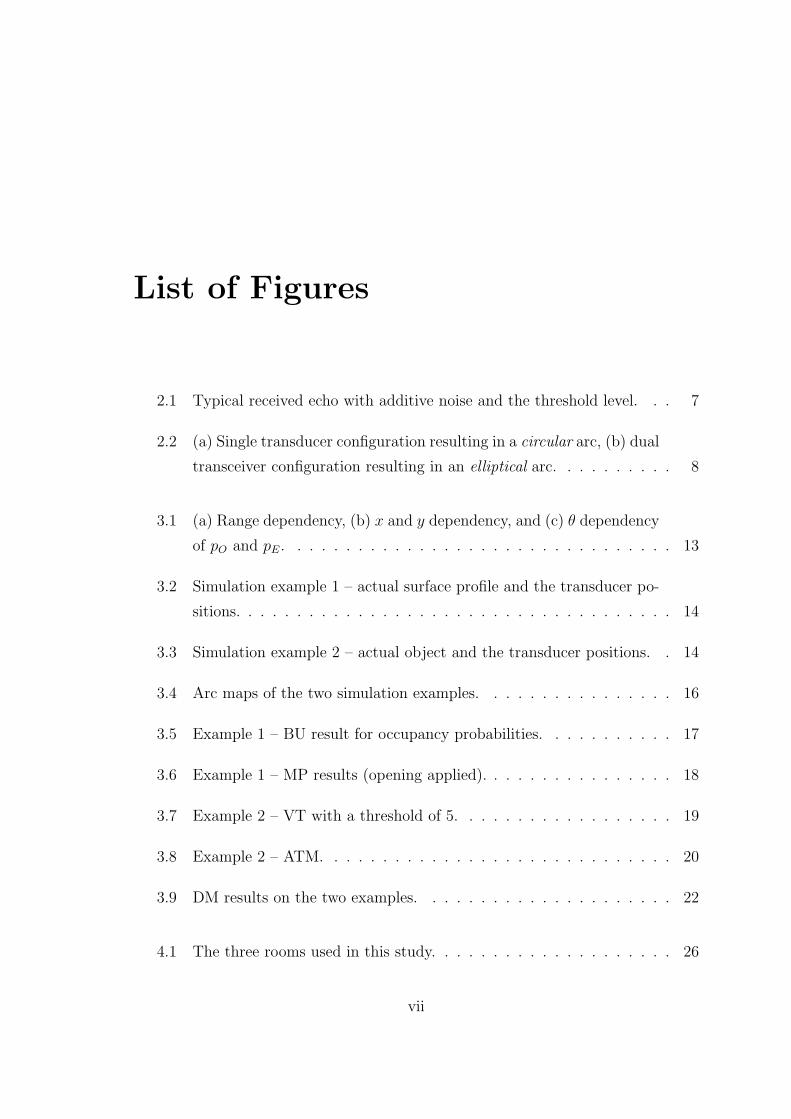
List of Figures
2.1 Typical received echo with additive noise and the threshold level. . . 7
2.2 (a) Single transducer configuration resulting in a circular arc, (b) dual
transceiver configuration resulting in an elliptical arc. . . . . . . . . . 8
3.1 (a) Range dependency, (b) x and y dependency, and (c) θ dependency
of pO and pE. . . . . . . . . . . . . . . . . . . . . . . . . . . . . . . . 13
3.2 Simulation example 1 – actual surface profile and the transducer po-
sitions. . . . . . . . . . . . . . . . . . . . . . . . . . . . . . . . . . . . 14
3.3 Simulation example 2 – actual object and the transducer positions. . 14
3.4 Arc maps of the two simulation examples. . . . . . . . . . . . . . . . 16
3.5 Example 1 – BU result for occupancy probabilities. . . . . . . . . . . 17
3.6 Example 1 – MP results (opening applied). . . . . . . . . . . . . . . . 18
3.7 Example 2 – VT with a threshold of 5. . . . . . . . . . . . . . . . . . 19
3.8 Example 2 – ATM. . . . . . . . . . . . . . . . . . . . . . . . . . . . . 20
3.9 DM results on the two examples. . . . . . . . . . . . . . . . . . . . . 22
4.1 The three rooms used in this study. . . . . . . . . . . . . . . . . . . . 26
vii
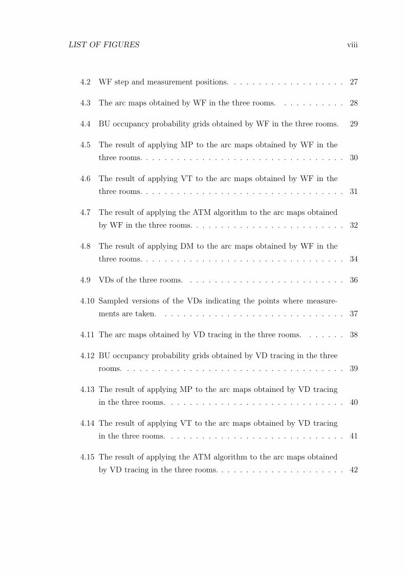
LIST OF FIGURES viii
4.2 WF step and measurement positions. . . . . . . . . . . . . . . . . . . 27
4.3 The arc maps obtained by WF in the three rooms. . . . . . . . . . . 28
4.4 BU occupancy probability grids obtained by WF in the three rooms. 29
4.5 The result of applying MP to the arc maps obtained by WF in the
three rooms. . . . . . . . . . . . . . . . . . . . . . . . . . . . . . . . . 30
4.6 The result of applying VT to the arc maps obtained by WF in the
three rooms. . . . . . . . . . . . . . . . . . . . . . . . . . . . . . . . . 31
4.7 The result of applying the ATM algorithm to the arc maps obtained
by WF in the three rooms. . . . . . . . . . . . . . . . . . . . . . . . . 32
4.8 The result of applying DM to the arc maps obtained by WF in the
three rooms. . . . . . . . . . . . . . . . . . . . . . . . . . . . . . . . . 34
4.9 VDs of the three rooms. . . . . . . . . . . . . . . . . . . . . . . . . . 36
4.10 Sampled versions of the VDs indicating the points where measure-
ments are taken. . . . . . . . . . . . . . . . . . . . . . . . . . . . . . 37
4.11 The arc maps obtained by VD tracing in the three rooms. . . . . . . 38
4.12 BU occupancy probability grids obtained by VD tracing in the three
rooms. . . . . . . . . . . . . . . . . . . . . . . . . . . . . . . . . . . . 39
4.13 The result of applying MP to the arc maps obtained by VD tracing
in the three rooms. . . . . . . . . . . . . . . . . . . . . . . . . . . . . 40
4.14 The result of applying VT to the arc maps obtained by VD tracing
in the three rooms. . . . . . . . . . . . . . . . . . . . . . . . . . . . . 41
4.15 The result of applying the ATM algorithm to the arc maps obtained
by VD tracing in the three rooms. . . . . . . . . . . . . . . . . . . . . 42

LIST OF FIGURES ix
4.16 The result of applying DM to the arc maps obtained by VD tracing
in the three rooms. . . . . . . . . . . . . . . . . . . . . . . . . . . . . 43
A.1 Geometry of the problem with the given sensor pair when the target
is a plane (adopted from [1]). . . . . . . . . . . . . . . . . . . . . . . 50
B.1 WF algorithm flowchart. . . . . . . . . . . . . . . . . . . . . . . . . . 54

List of Tables
3.1 Error criteria for the two simulation examples. . . . . . . . . . . . . . 23
4.1 Mean absolute error – indoor simulations with WF. . . . . . . . . . . 44
4.2 Fill ratio – indoor simulations with WF. . . . . . . . . . . . . . . . . 45
4.3 CPU time – indoor simulations with WF. . . . . . . . . . . . . . . . . 45
4.4 Mean absolute error – indoor simulations with VD tracing. . . . . . . 45
4.5 Fill ratio – indoor simulations with VD tracing. . . . . . . . . . . . . 46
4.6 CPU time – indoor simulations with VD tracing. . . . . . . . . . . . 46
x
Chapter 1
Introduction
The basic awareness of the surrounding environment is a notable feature of intelligent
mobile robots. This awareness can be accomplished by means of simple sensor
utilization and processing of obtained sensory data according to the perceptive needs
of the robot such as navigation, tracking and/or avoidance of targets, path-planning
and localization. In static but unknown environments, where an a priori map of the
working area is not available, or in dynamically changing environments, the robot
is supposed to build an accurate map of its surroundings by using the sensory data
it gathers for autonomous operation. Therefore, the selection of an appropriate
map-building scheme is an important issue.
Ultrasonic sensors have been widely utilized in robotic applications due to their
accurate range measurements and low cost. The frequency range at which air-borne
ultrasonic transducers operate is associated with a large beamwidth that results in
angular uncertainty of the echo-producing target. Thus having an intrinsic uncer-
tainty of the actual angular direction of the range measurement and being prone to
various phenomena such as multiple and higher-order reflections and cross-talk be-
tween transducers, a considerable amount of modeling, processing and interpretation
of the sensory data is necessary.
Being a low-cost solution to the sensory perception problem with robust charac-
teristics, ultrasonic sensors have been widely used in map-building applications [2,3].
1
CHAPTER 1. INTRODUCTION 2
Grid-based and feature-based approaches have been in use to represent the environ-
ment since the early days of map building. The occupancy grids were introduced
in [4] and a Bayesian update scheme for cell occupancy probabilities was suggested.
In [5], a dynamic map-building method via correlating fixed beacons was developed
and map building in dynamic environments has been investigated in a number of
studies [6, 7].
As an alternative to grid-based approaches to map building and world represen-
tation for mobile robots, feature-based approaches have also been popular [5,6,8,9].
In this school of map representation, the world model is described in terms of natural
features of the environment (e.g., planes, corners, edges and cylinders) the orienta-
tion and position of which are known [10, 11]. The echo patterns of planes, corners
and edges were first modeled in [10] and they have been used as natural beacons for
map building in [6]. Planes and corners were differentiated by using the amplitude
and time-of-flight characteristics of the ultrasonic data [11]. In [12] and [13], the
complete waveform of the received echo is processed using matched filters in order
to achieve higher accuracy. In [14], maximum likelihood estimation is employed in
a 3-D setting. Evidential reasoning was utilized in [1] in a multi-sensor fusion appli-
cation. In addition to map-building applications of ultrasonic target differentiation,
it was reported in [15] that an ultrasonic sensor mounted at the tip of a robot arm
could be used to differentiate coins and O-rings.
Map-building applications can also be classified according to the coverage scheme
employed. The systematic way the unknown environment to be mapped is covered,
or motion planning, may be roughly divided into three approaches. One method
of ground coverage scheme involves pseudo-random steps with collision avoidance
[16–18]. The more systematic wall following type coverage can further be divided
into two general cases: simple rule-based wall following [19] and potential field-based
wall following [20]. In the second case, each obstacle/wall creates a potential field
and the mobile platform aims at staying on constant potential lines. There also
exist different approaches to the wall-following problem that cannot be included
under the above two categories [21, 22], for example, those which employ fuzzy-
logic based control methods [23]. The third and most sophisticated coverage scheme
involved in map building is based on Voronoi diagrams that can be constructed
CHAPTER 1. INTRODUCTION 3
iteratively [24–26].
The main contribution of this thesis is that it provides a valuable comparison
between the performances of one newly proposed and four existing algorithms for
processing ultrasonic arc maps for map-building purposes. The comparison is based
on three different error criteria. Each method is found to have certain advantages
and disadvantages which make them suitable for map building under different con-
straints and requirements. The newly proposed method is promising as it intro-
duces a sense of direction in the data acquisition and processing. This is found to
be beneficial and the determination of such directional awareness is proved to be
cost-effective since most motion-planning approaches already involve a similar sense
of direction. The newly proposed method also results in the minimum mean abso-
lute error between the true map and constructed map. Another contribution of this
thesis is the comparison it provides between two different motion-planning schemes
which are wall following and Voronoi diagram tracing for map-building applications.
Even though the simulation results demonstrated in this thesis are solely based on
ultrasonic data and map-building applications, the same approach can conveniently
be extended to other sensing modalities such as radar and infrared, as well as other
mobile robot applications.
This thesis is organized as follows: In Chapter 2, the basics of ultrasonic sensing
are reviewed. Descriptions and a basic comparison of five different map-building
techniques are given in Chapter 3, through two simulation examples. Chapter 4
expands the comparison to indoor map-building scenarios. The results are presented
and discussed at the end of each chapter with numerical success measures, while final
notes, conclusions, and future work form Chapter 5.
Chapter 2
Basics of Ultrasonic Sensing
This chapter reviews the basics of ultrasonic sensing, in particular, time-of-flight
(TOF) measurement using ultrasonic sensors. Operating principles, governing equa-
tions and uncertainties related to ultrasonic sensors are summarized.
2.1 Ultrasonic Transducers
Ultrasonic sensors operate at frequencies between 20–300 kHz. They perform trans-
duction by converting electrical signals to acoustical waves and converting the re-
ceived reflection of the transmitted waves back into electrical signals. Acoustical
waves transmitted by the transducer exhibit different characteristics in the near
field, where Fresnel diffraction is dominant, and the far field, where Fraunhofer
diffraction is dominant. According to the harmonically vibrating circular piston
model of the transducer in the near field [27], the beam is confined to a cylinder
with radius a, which is the radius of the transducer aperture. The length of this field
is rmin = (4a2−λ2)
4λ∼= a2
λfrom the face of the transducer where λ is the wavelength
of the acoustic transmission. On the other hand, the beam is confined to a cone
with angle 2θ0 in the far field. We are mainly interested in the far field since the
range measurements of interest correspond to this region and the complexity of the
acoustical interference is high in the near field [27].
4
CHAPTER 2. BASICS OF ULTRASONIC SENSING 5
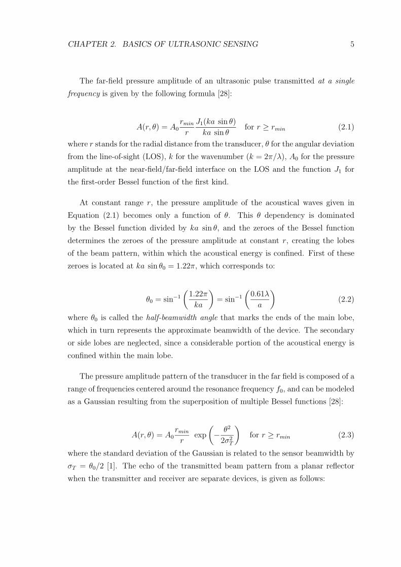
The far-field pressure amplitude of an ultrasonic pulse transmitted at a single
frequency is given by the following formula [28]:
A(r, θ) = A0rmin
r
J1(ka sin θ)
ka sin θfor r ≥ rmin (2.1)
where r stands for the radial distance from the transducer, θ for the angular deviation
from the line-of-sight (LOS), k for the wavenumber (k = 2π/λ), A0 for the pressure
amplitude at the near-field/far-field interface on the LOS and the function J1 for
the first-order Bessel function of the first kind.
At constant range r, the pressure amplitude of the acoustical waves given in
Equation (2.1) becomes only a function of θ. This θ dependency is dominated
by the Bessel function divided by ka sin θ, and the zeroes of the Bessel function
determines the zeroes of the pressure amplitude at constant r, creating the lobes
of the beam pattern, within which the acoustical energy is confined. First of these
zeroes is located at ka sin θ0 = 1.22π, which corresponds to:
θ0 = sin−1
(
1.22π
ka
)
= sin−1
(
0.61λ
a
)
(2.2)
where θ0 is called the half-beamwidth angle that marks the ends of the main lobe,
which in turn represents the approximate beamwidth of the device. The secondary
or side lobes are neglected, since a considerable portion of the acoustical energy is
confined within the main lobe.
The pressure amplitude pattern of the transducer in the far field is composed of a
range of frequencies centered around the resonance frequency f0, and can be modeled
as a Gaussian resulting from the superposition of multiple Bessel functions [28]:
A(r, θ) = A0rmin
rexp
(
−θ2
2σ2T
)
for r ≥ rmin (2.3)
where the standard deviation of the Gaussian is related to the sensor beamwidth by
σT = θ0/2 [1]. The echo of the transmitted beam pattern from a planar reflector
when the transmitter and receiver are separate devices, is given as follows:
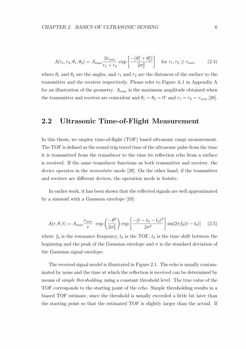
CHAPTER 2. BASICS OF ULTRASONIC SENSING 6
A(r1, r2, θ1, θ2) = Amax
2rmin
r1 + r2
exp
[
−(θ21 + θ2
2)
2σ2T
]
for r1, r2 ≥ rmin (2.4)
where θ1 and θ2 are the angles, and r1 and r2 are the distances of the surface to the
transmitter and the receiver respectively. Please refer to Figure A.1 in Appendix A
for an illustration of the geometry. Amax is the maximum amplitude obtained when
the transmitter and receiver are coincident and θ1 = θ2 = 0◦ and r1 = r2 = rmin [28].
2.2 Ultrasonic Time-of-Flight Measurement
In this thesis, we employ time-of-flight (TOF) based ultrasonic range measurement.
The TOF is defined as the round-trip travel time of the ultrasonic pulse from the time
it is transmitted from the transducer to the time its reflection echo from a surface
is received. If the same transducer functions as both transmitter and receiver, the
device operates in the monostatic mode [29]. On the other hand, if the transmitter
and receiver are different devices, the operation mode is bistatic.
In earlier work, it has been shown that the reflected signals are well approximated
by a sinusoid with a Gaussian envelope [10]:
A(r, θ, t) = Amax
rmin
rexp
(
−θ2
2σ2T
)
exp
[
−(t − t0 − td)2
2σ2
]
sin[2πf0(t − t0)] (2.5)
where f0 is the resonance frequency, t0 is the TOF, td is the time shift between the
beginning and the peak of the Gaussian envelope and σ is the standard deviation of
the Gaussian signal envelope.
The received signal model is illustrated in Figure 2.1. The echo is usually contam-
inated by noise and the time at which the reflection is received can be determined by
means of simple thresholding, using a constant threshold level. The true value of the
TOF corresponds to the starting point of the echo. Simple thresholding results in a
biased TOF estimate, since the threshold is usually exceeded a little bit later than
the starting point so that the estimated TOF is slightly larger than the actual. If
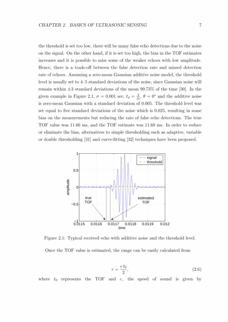
CHAPTER 2. BASICS OF ULTRASONIC SENSING 7
the threshold is set too low, there will be many false echo detections due to the noise
on the signal. On the other hand, if it is set too high, the bias in the TOF estimates
increases and it is possible to miss some of the weaker echoes with low amplitude.
Hence, there is a trade-off between the false detection rate and missed detection
rate of echoes. Assuming a zero-mean Gaussian additive noise model, the threshold
level is usually set to 4–5 standard deviations of the noise, since Gaussian noise will
remain within ±3 standard deviations of the mean 99.73% of the time [30]. In the
given example in Figure 2.1, σ = 0.001 sec, td = 3f0
, θ = 0◦ and the additive noise
is zero-mean Gaussian with a standard deviation of 0.005. The threshold level was
set equal to five standard deviations of the noise which is 0.025, resulting in some
bias on the measurements but reducing the rate of false echo detections. The true
TOF value was 11.66 ms, and the TOF estimate was 11.68 ms. In order to reduce
or eliminate the bias, alternatives to simple thresholding such as adaptive, variable
or double thresholding [31] and curve-fitting [32] techniques have been proposed.
0.0115 0.0116 0.0117 0.0118 0.0119 0.012−1
−0.5
0
0.5
1
time
ampl
itude
signalthreshold
trueTOF
estimatedTOF
Figure 2.1: Typical received echo with additive noise and the threshold level.
Once the TOF value is estimated, the range can be easily calculated from
r =c t02
, (2.6)
where t0 represents the TOF and c, the speed of sound is given by
CHAPTER 2. BASICS OF ULTRASONIC SENSING 8
����������������������������������������������������������������������������������������������������������������
����������������������������������������������������������������������������������������������������������������
T/R
line−of−sight
surface
r
sensitivityregion
circular arc
r_min
ultrasonic transducer
(a) monostatic mode
����������������������������������������������������������������������������������������������������������������
����������������������������������������������������������������������������������������������������������������
sensitivityregion
surface
joint
T Rultrasonic transducer pair
elliptical arc
(b) bistatic mode
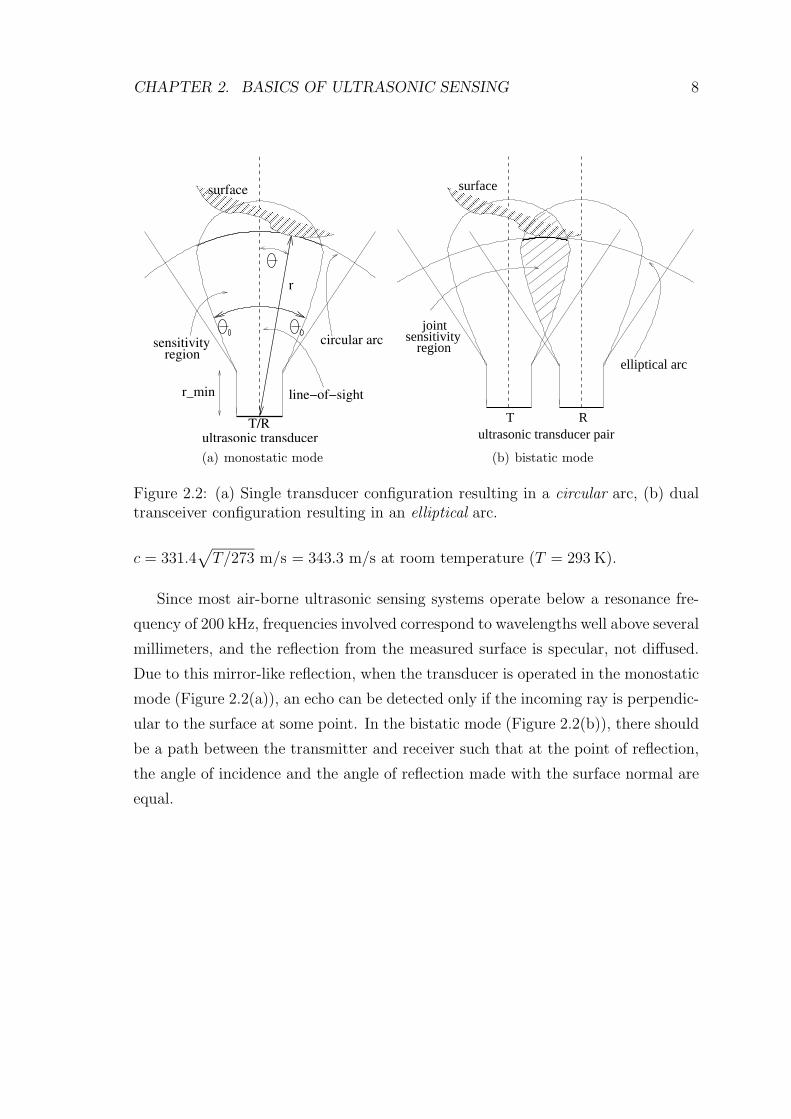
Figure 2.2: (a) Single transducer configuration resulting in a circular arc, (b) dualtransceiver configuration resulting in an elliptical arc.
c = 331.4√
T/273 m/s = 343.3 m/s at room temperature (T = 293 K).
Since most air-borne ultrasonic sensing systems operate below a resonance fre-
quency of 200 kHz, frequencies involved correspond to wavelengths well above several
millimeters, and the reflection from the measured surface is specular, not diffused.
Due to this mirror-like reflection, when the transducer is operated in the monostatic
mode (Figure 2.2(a)), an echo can be detected only if the incoming ray is perpendic-
ular to the surface at some point. In the bistatic mode (Figure 2.2(b)), there should
be a path between the transmitter and receiver such that at the point of reflection,
the angle of incidence and the angle of reflection made with the surface normal are
equal.
CHAPTER 2. BASICS OF ULTRASONIC SENSING 9
2.3 Representing Angular Uncertainty by Arc
Maps
In this study, simple ultrasonic range sensors are modeled that measure the TOF and
provide a range measurement according to Equation (2.6). Although such devices
return accurate range data, typically they cannot provide direct information on the
angular position of the point on the surface from which the reflection was obtained.
Most commonly, the large beamwidth of the transducer is accepted as a device limi-
tation that determines the angular resolving power of the system, and the reflection
point is assumed to be along the LOS. According to this naive approach, a simple
mark is placed along the LOS of the transducer at the measured range, resulting in
inaccurate maps with large angular errors. Alternatively, the angular uncertainty in
the range measurements has been represented by regions of constant depth [33] and
ultrasonic arc maps [34,35] that represent the angular uncertainty while preserving
more information. This is done by drawing arcs spanning the beamwidth of the
sensor at the measured range, representing the angular uncertainty of the object
location and indicating that the echo-producing object can lie anywhere on the arc.
Thus, when the same transducer transmits and receives, all that is known is that the
reflection point lies on a circular arc of radius r, as illustrated in Figure 2.2(a). More
generally, when one transducer transmits and another receives, it is known that the
reflection point lies on the arc of an ellipse whose focal points are the transmitting
and receiving elements (Figure 2.2(b)). The arcs are tangent to the reflecting surface
at the actual point(s) of reflection. Arc segments near the actual reflection points
tend to reinforce each other. Arc segments not actually corresponding to any re-
flections and simply representing the angular uncertainty of the transducers remain
more sparse and isolated. Similarly, those arcs caused by higher-order reflections,
crosstalk, and noise also remain sparse and lack reinforcement. By combining the
information inherent in a large number of such arcs, angular resolution far exceeding
the beamwidth is obtained.
Apart from the wide beamwidth, another commonly noted disadvantage of ultra-
sonic range sensors is the difficulty associated with interpreting spurious readings,
crosstalk, higher-order, and multiple reflections. The proposed method is capable of
CHAPTER 2. BASICS OF ULTRASONIC SENSING 10
effectively suppressing the first three of these, and, although not implemented here,
it would have the intrinsic ability to process echoes returning from surface features
further away than the nearest (i.e., multiple reflections) informatively.
The device that is modeled and used in this study is the Polaroid 6500 series
transducer [36] operating at a resonance frequency of f0 = 49.4 kHz, corresponding
to a wavelength of λ = c/f0 = 6.9 mm. The half beamwidth of the transducer is θ0 =
±12.5◦, the transducer aperture radius is a = 2 cm and rmin = 5.7 cm. We use a pair
of these transducers, with a center-to-center separation of 9 cm. Each transducer
is fired in sequence and both transducers detect the resulting echoes. After a pulse
is transmitted, if echoes are detected at both transducers, this corresponds to one
circular and one elliptical arc. Hence, with two transducers each firing in its own
turn, at most four arcs are obtained at each position of the transducer pair. The
signal models of these echoes are provided in Appendix A.
In the following chapters, we introduce a new method to process these arc maps
and compare it with the existing methods.
Chapter 3
Algorithm Descriptions
In this work, we implemented and compared the following algorithms for processing
arc maps, the last of which is developed in this thesis:
• Bayesian update scheme [3],
• morphological processing of arc maps [34,35],
• voting and thresholding of arc maps [37,38],
• arc-transversal median algorithm [39],
• and directional maximum algorithm.
Different arc maps, each corresponding to a certain set of TOF measurements is
processed by each method and the results are compared.
3.1 Bayesian Update (BU)
Occupancy grids representing the probability of occupancy are introduced primar-
ily by Elfes and Moravec [3, 4]. A Bayesian update scheme for these occupancy
11
CHAPTER 3. ALGORITHM DESCRIPTIONS 12
grids by using ultrasonic sensor data was suggested in [3] and is included in this
thesis as an earlier example of related work. Starting with a blank or completely
uncertain occupancy grid, each range measurement updates the grid formation in a
Bayesian manner. For a certain measurement, the following sensor characteristics
and obtained data are listed for each pixel P (x, y) of the map to be updated:
• r range measurement returned by the ultrasonic sensor
• rmin lower range threshold (near-field limit)
• rǫ maximum ultrasonic range measurement error
• θ0 sensor half-beamwidth angle
• 2θ0 beamwidth angle subtending the main lobe of the sensitivity region
• S = (xs, ys) position of the ultrasonic sensor
• σ distance from P (x, y) to S = (xs, ys)
Occupancy probability of the scanned pixels are defined over two distinct prob-
ability measures: (pE, probability of emptiness and pO, probability of occupancy).
These probability density functions are defined as follows:
pE(x, y) = p[point (x, y) is empty]
= Er(σ) · Ea(θ)
where Er(σ) and Ea(θ) are respectively the range and angle dependency of the
probability density function for emptiness, given by:
Er(σ) =
{
1 − [(σ − rmin)/(r − rǫ − rmin)]2 for σ ∈ [rmin, r − rǫ],
0 otherwise,
and
Ea(θ) = 1 − (θ/θ0)2, for θ ∈ [−θ0, θ0].
CHAPTER 3. ALGORITHM DESCRIPTIONS 13
Likewise, pO is defined as:
pO(x, y) = p[position (x, y) is occupied]
= Or(σ) · Oa(θ)
where Or(σ) and Oa(θ) are respectively the range and angle dependency of the
probability density function for occupancy, and defined as:
Or(σ) =
{
1 − [(σ − r)/rǫ]2, for σ ∈ [r − rǫ, r + rǫ]
0 otherwise,
and
Oa(θ) = 1 − (θ/θ0)2, for θ ∈ [−θ0, θ0].
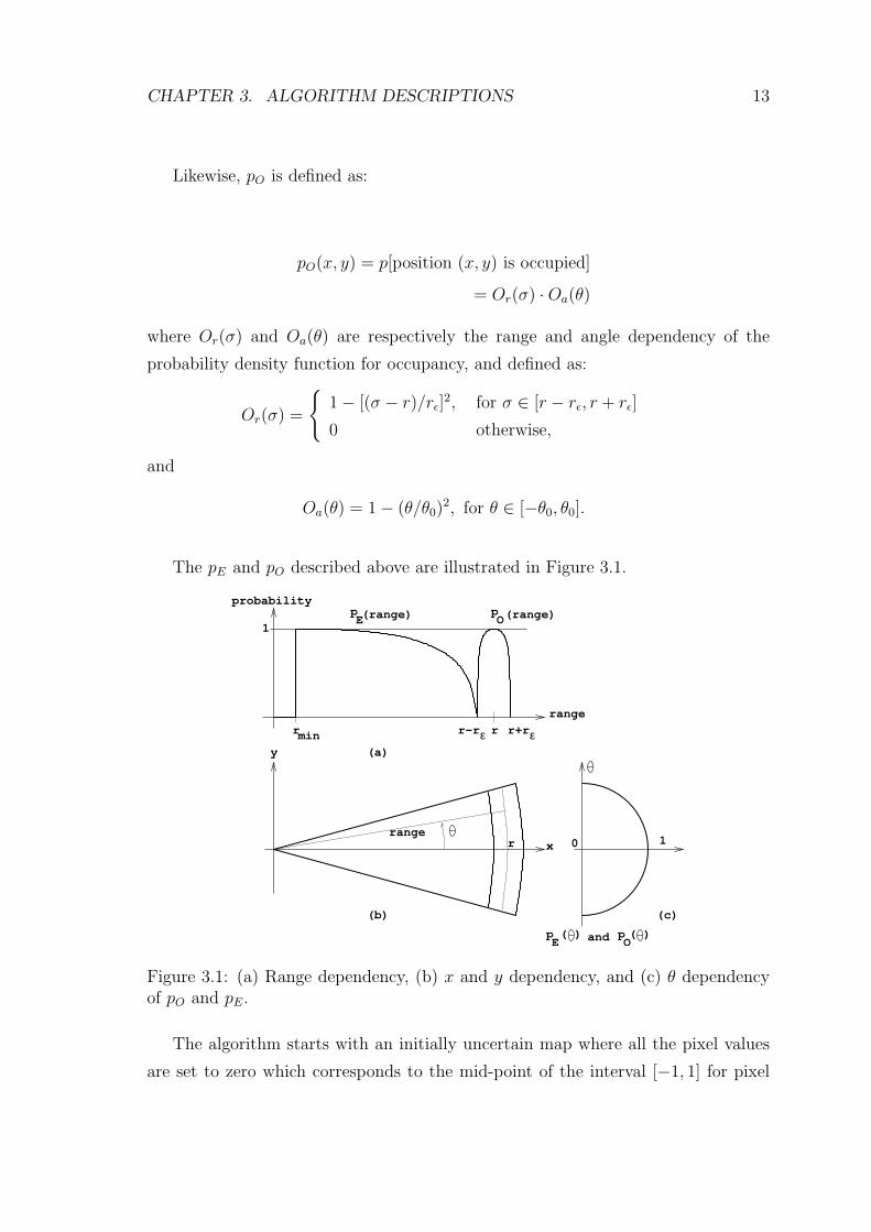
The pE and pO described above are illustrated in Figure 3.1.
rmin
r
EpO(range)
range
1
r x10
( )E
pprobability
(range)
ε εr−r r+r
y
range
( )Opp and
(a)
(b) (c)
Figure 3.1: (a) Range dependency, (b) x and y dependency, and (c) θ dependencyof pO and pE.
The algorithm starts with an initially uncertain map where all the pixel values
are set to zero which corresponds to the mid-point of the interval [−1, 1] for pixel
CHAPTER 3. ALGORITHM DESCRIPTIONS 14
values. For each range measurement, pE and pO values are calculated for the cells
inside the field of view of the transducer by using the above formulas. The following
Bayesian update rules are used to update the existing values in the cell array:
pE(cell) := pE(cell) + pE(reading) − pE(cell) × pE(reading)
pO(cell) := pO(cell) + pO(reading) − pO(cell) × pO(reading)
The map of the environment is built by iteratively updating the contents of each cell
via a number of range measurements. In the end, pE and pO arrays form modified
probability distribution functions that vary between –1 and 1.
pixels
pixe
ls
200 400 600 800
0
100
200
300
400
500
600
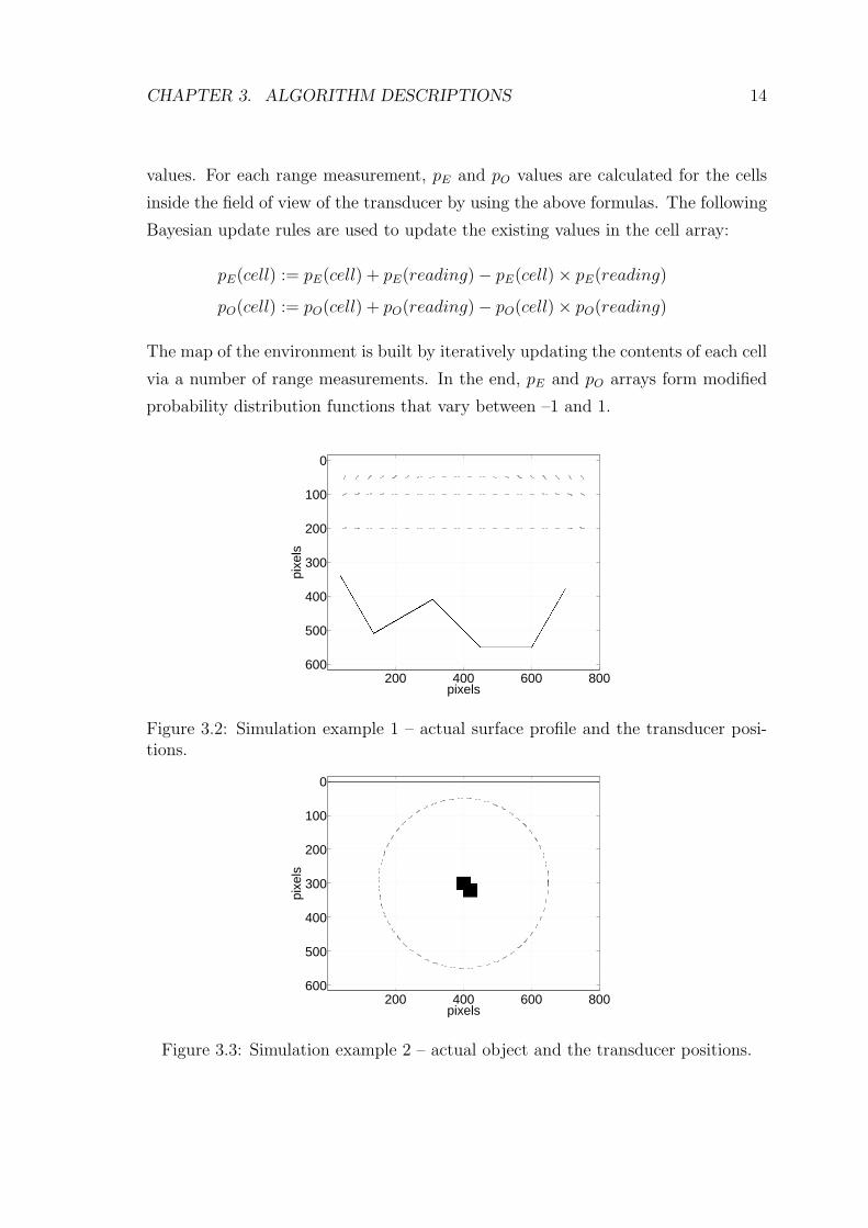
Figure 3.2: Simulation example 1 – actual surface profile and the transducer posi-tions.
pixels
pixe
ls
200 400 600 800
0
100
200
300
400
500
600
Figure 3.3: Simulation example 2 – actual object and the transducer positions.
CHAPTER 3. ALGORITHM DESCRIPTIONS 15
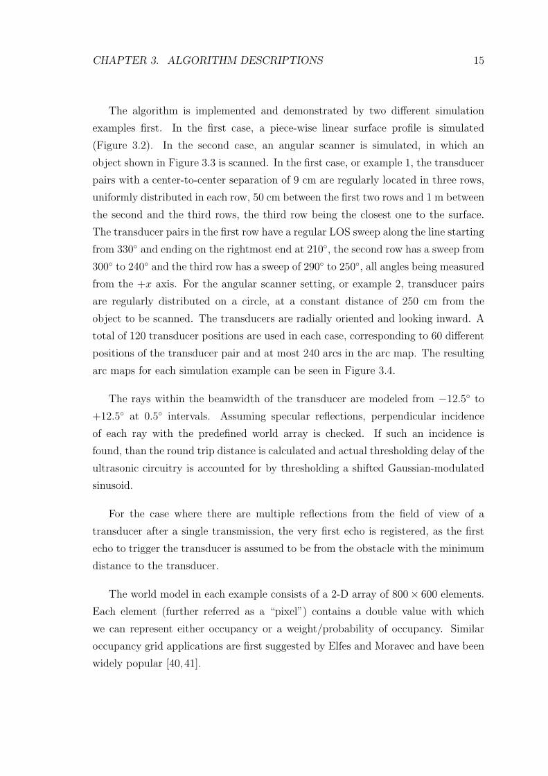
The algorithm is implemented and demonstrated by two different simulation
examples first. In the first case, a piece-wise linear surface profile is simulated
(Figure 3.2). In the second case, an angular scanner is simulated, in which an
object shown in Figure 3.3 is scanned. In the first case, or example 1, the transducer
pairs with a center-to-center separation of 9 cm are regularly located in three rows,
uniformly distributed in each row, 50 cm between the first two rows and 1 m between
the second and the third rows, the third row being the closest one to the surface.
The transducer pairs in the first row have a regular LOS sweep along the line starting
from 330◦ and ending on the rightmost end at 210◦, the second row has a sweep from
300◦ to 240◦ and the third row has a sweep of 290◦ to 250◦, all angles being measured
from the +x axis. For the angular scanner setting, or example 2, transducer pairs
are regularly distributed on a circle, at a constant distance of 250 cm from the
object to be scanned. The transducers are radially oriented and looking inward. A
total of 120 transducer positions are used in each case, corresponding to 60 different
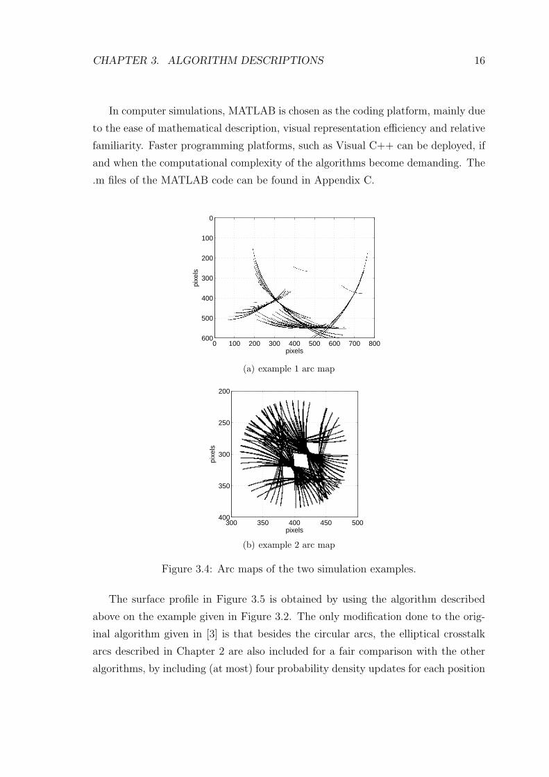
positions of the transducer pair and at most 240 arcs in the arc map. The resulting
arc maps for each simulation example can be seen in Figure 3.4.
The rays within the beamwidth of the transducer are modeled from −12.5◦ to
+12.5◦ at 0.5◦ intervals. Assuming specular reflections, perpendicular incidence
of each ray with the predefined world array is checked. If such an incidence is
found, than the round trip distance is calculated and actual thresholding delay of the
ultrasonic circuitry is accounted for by thresholding a shifted Gaussian-modulated
sinusoid.
For the case where there are multiple reflections from the field of view of a
transducer after a single transmission, the very first echo is registered, as the first
echo to trigger the transducer is assumed to be from the obstacle with the minimum
distance to the transducer.
The world model in each example consists of a 2-D array of 800× 600 elements.
Each element (further referred as a “pixel”) contains a double value with which
we can represent either occupancy or a weight/probability of occupancy. Similar
occupancy grid applications are first suggested by Elfes and Moravec and have been
widely popular [40,41].
CHAPTER 3. ALGORITHM DESCRIPTIONS 16
In computer simulations, MATLAB is chosen as the coding platform, mainly due
to the ease of mathematical description, visual representation efficiency and relative
familiarity. Faster programming platforms, such as Visual C++ can be deployed, if
and when the computational complexity of the algorithms become demanding. The
.m files of the MATLAB code can be found in Appendix C.
pixels
pixe
ls
0 100 200 300 400 500 600 700 800
0
100
200
300
400
500
600
(a) example 1 arc map
pixels
pixe
ls
300 350 400 450 500
200
250
300
350
400
(b) example 2 arc map
Figure 3.4: Arc maps of the two simulation examples.
The surface profile in Figure 3.5 is obtained by using the algorithm described
above on the example given in Figure 3.2. The only modification done to the orig-
inal algorithm given in [3] is that besides the circular arcs, the elliptical crosstalk
arcs described in Chapter 2 are also included for a fair comparison with the other
algorithms, by including (at most) four probability density updates for each position
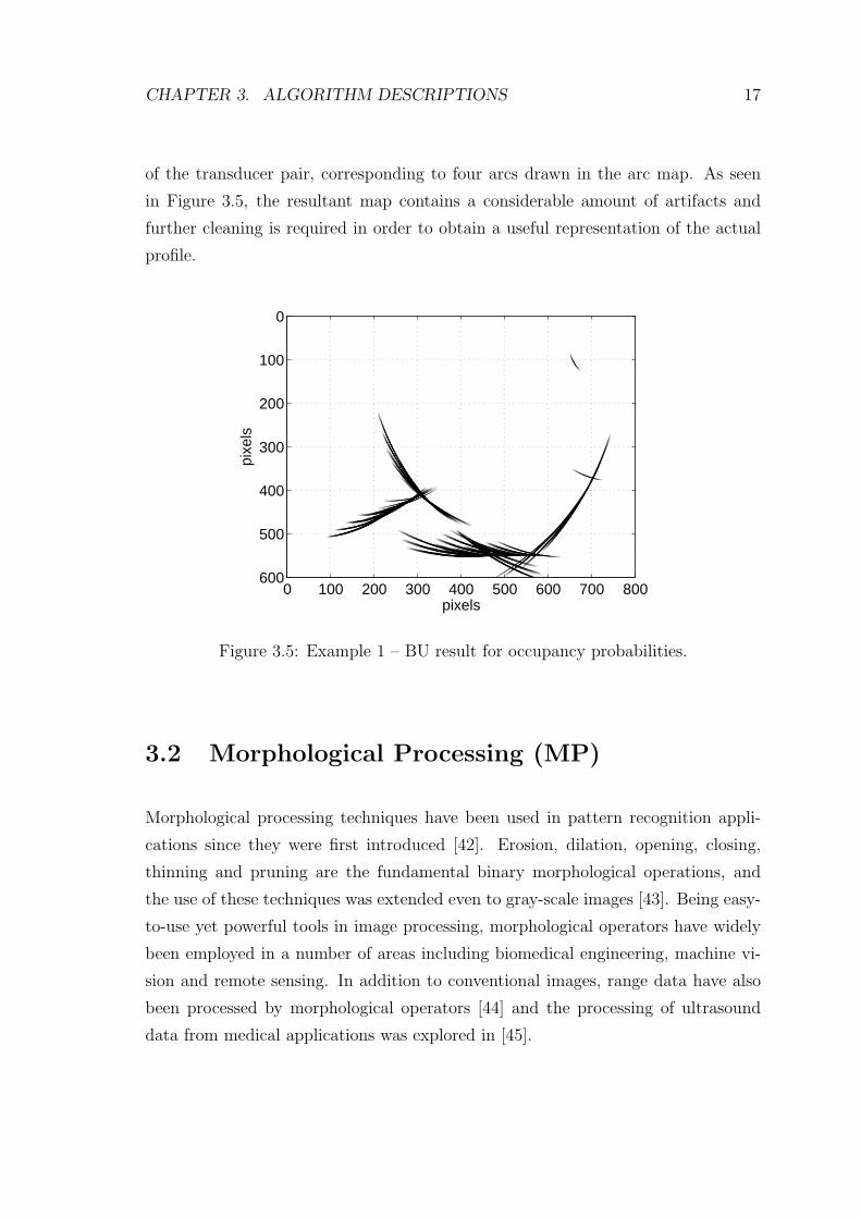
CHAPTER 3. ALGORITHM DESCRIPTIONS 17
of the transducer pair, corresponding to four arcs drawn in the arc map. As seen
in Figure 3.5, the resultant map contains a considerable amount of artifacts and
further cleaning is required in order to obtain a useful representation of the actual
profile.
pixels
pixe
ls
0 100 200 300 400 500 600 700 800
0
100
200
300
400
500
600
Figure 3.5: Example 1 – BU result for occupancy probabilities.
3.2 Morphological Processing (MP)
Morphological processing techniques have been used in pattern recognition appli-
cations since they were first introduced [42]. Erosion, dilation, opening, closing,
thinning and pruning are the fundamental binary morphological operations, and
the use of these techniques was extended even to gray-scale images [43]. Being easy-
to-use yet powerful tools in image processing, morphological operators have widely
been employed in a number of areas including biomedical engineering, machine vi-
sion and remote sensing. In addition to conventional images, range data have also
been processed by morphological operators [44] and the processing of ultrasound
data from medical applications was explored in [45].
CHAPTER 3. ALGORITHM DESCRIPTIONS 18
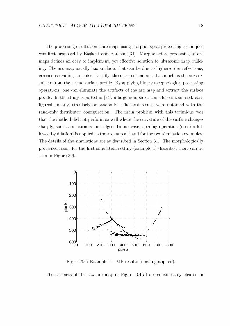
The processing of ultrasonic arc maps using morphological processing techniques
was first proposed by Baskent and Barshan [34]. Morphological processing of arc
maps defines an easy to implement, yet effective solution to ultrasonic map build-
ing. The arc map usually has artifacts that can be due to higher-order reflections,
erroneous readings or noise. Luckily, these are not enhanced as much as the arcs re-
sulting from the actual surface profile. By applying binary morphological processing
operations, one can eliminate the artifacts of the arc map and extract the surface
profile. In the study reported in [34], a large number of transducers was used, con-
figured linearly, circularly or randomly. The best results were obtained with the
randomly distributed configuration. The main problem with this technique was
that the method did not perform so well where the curvature of the surface changes
sharply, such as at corners and edges. In our case, opening operation (erosion fol-
lowed by dilation) is applied to the arc map at hand for the two simulation examples.
The details of the simulations are as described in Section 3.1. The morphologically
processed result for the first simulation setting (example 1) described there can be
seen in Figure 3.6.
pixels
pixe
ls
0 100 200 300 400 500 600 700 800
0
100
200
300
400
500
600
Figure 3.6: Example 1 – MP results (opening applied).
The artifacts of the raw arc map of Figure 3.4(a) are considerably cleared in
CHAPTER 3. ALGORITHM DESCRIPTIONS 19
Figure 3.6. However, the corners are still distorted while edges have major discon-
tinuities.
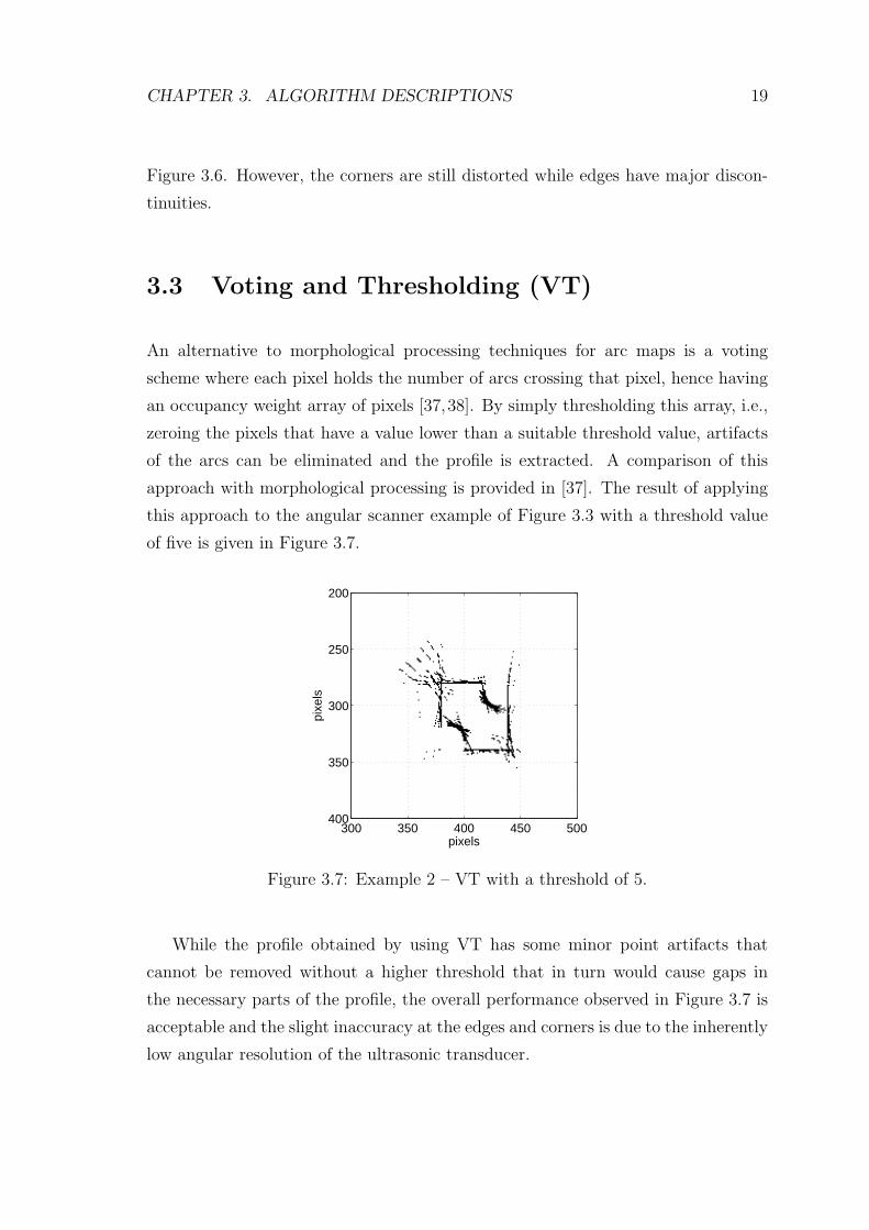
3.3 Voting and Thresholding (VT)
An alternative to morphological processing techniques for arc maps is a voting
scheme where each pixel holds the number of arcs crossing that pixel, hence having
an occupancy weight array of pixels [37,38]. By simply thresholding this array, i.e.,
zeroing the pixels that have a value lower than a suitable threshold value, artifacts
of the arcs can be eliminated and the profile is extracted. A comparison of this
approach with morphological processing is provided in [37]. The result of applying
this approach to the angular scanner example of Figure 3.3 with a threshold value
of five is given in Figure 3.7.
pixels
pixe
ls
300 350 400 450 500
200
250
300
350
400
Figure 3.7: Example 2 – VT with a threshold of 5.
While the profile obtained by using VT has some minor point artifacts that
cannot be removed without a higher threshold that in turn would cause gaps in
the necessary parts of the profile, the overall performance observed in Figure 3.7 is
acceptable and the slight inaccuracy at the edges and corners is due to the inherently
low angular resolution of the ultrasonic transducer.
CHAPTER 3. ALGORITHM DESCRIPTIONS 20
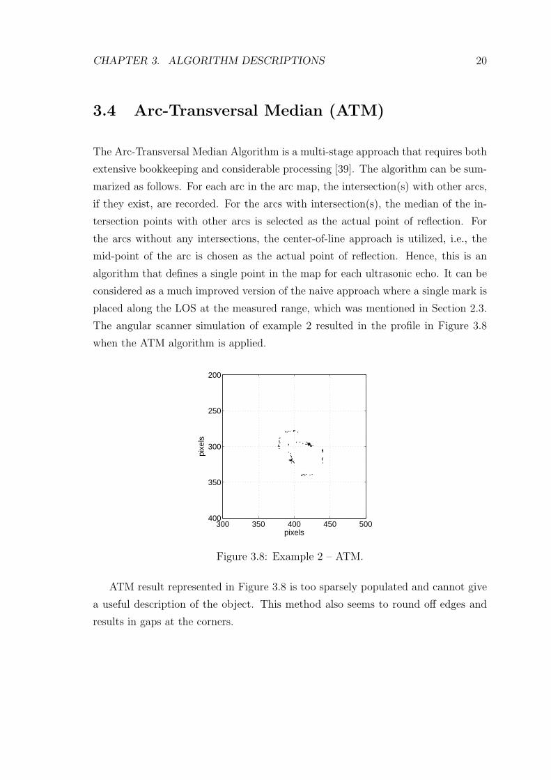
3.4 Arc-Transversal Median (ATM)
The Arc-Transversal Median Algorithm is a multi-stage approach that requires both
extensive bookkeeping and considerable processing [39]. The algorithm can be sum-
marized as follows. For each arc in the arc map, the intersection(s) with other arcs,
if they exist, are recorded. For the arcs with intersection(s), the median of the in-
tersection points with other arcs is selected as the actual point of reflection. For
the arcs without any intersections, the center-of-line approach is utilized, i.e., the
mid-point of the arc is chosen as the actual point of reflection. Hence, this is an
algorithm that defines a single point in the map for each ultrasonic echo. It can be
considered as a much improved version of the naive approach where a single mark is
placed along the LOS at the measured range, which was mentioned in Section 2.3.
The angular scanner simulation of example 2 resulted in the profile in Figure 3.8
when the ATM algorithm is applied.
pixels
pixe
ls
300 350 400 450 500
200
250
300
350
400
Figure 3.8: Example 2 – ATM.
ATM result represented in Figure 3.8 is too sparsely populated and cannot give
a useful description of the object. This method also seems to round off edges and
results in gaps at the corners.
CHAPTER 3. ALGORITHM DESCRIPTIONS 21
3.5 Directional Maximum (DM)
In this method, we assume that we have a designated direction-of-interest (DOI)
in any map-building scenario. This direction may be based on prior knowledge,
or it can be predetermined by the map-building procedure as demonstrated in the
indoor map-building examples in the following chapter. For instance, in our profile
determination scenario (example 1), the vertical direction is the DOI, while in the
angular scanner case the DOI is the radial direction, which changes as the angular
position of the scanner head changes. If DOI is not known, it can be found from the
distribution of the data and is chosen perpendicular to the direction along which
the spread of the collected data is maximum.
Once the DOI is given or determined, the arc map that contains the artifacts is
scanned along this DOI; column-wise for the indoor profile case and radial direction-
wise for the angular scanner case. Each column/directional array is processed as to
leave only the directional maximum value and blank-out the rest of the pixels. If
there exist more than one pixel with the maximum value in the array, the algorithm
selects the one encountered first in the DOI. This step constitutes the actual artifact
removal step of the algorithm. As a final step, morphological processing is applied to
the arc maps of these two examples, consisting of applying the bridging and dilation
operations twice.
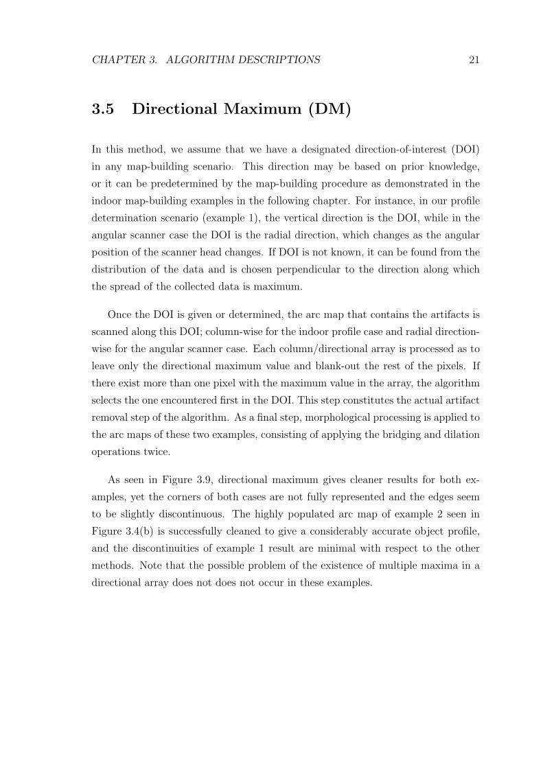
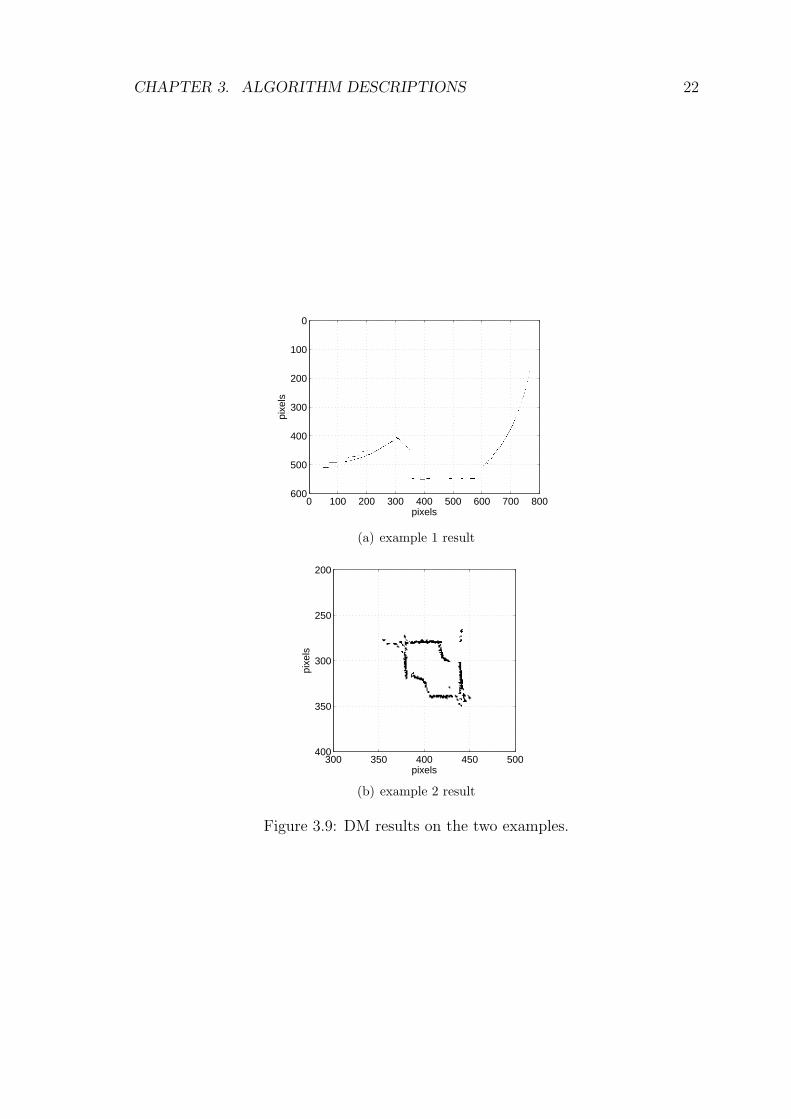
As seen in Figure 3.9, directional maximum gives cleaner results for both ex-
amples, yet the corners of both cases are not fully represented and the edges seem
to be slightly discontinuous. The highly populated arc map of example 2 seen in
Figure 3.4(b) is successfully cleaned to give a considerably accurate object profile,
and the discontinuities of example 1 result are minimal with respect to the other
methods. Note that the possible problem of the existence of multiple maxima in a
directional array does not does not occur in these examples.
CHAPTER 3. ALGORITHM DESCRIPTIONS 22
pixels
pixe
ls
0 100 200 300 400 500 600 700 800
0
100
200
300
400
500
600
(a) example 1 result
pixels
pixe
ls
300 350 400 450 500
200
250
300
350
400
(b) example 2 result
Figure 3.9: DM results on the two examples.
CHAPTER 3. ALGORITHM DESCRIPTIONS 23
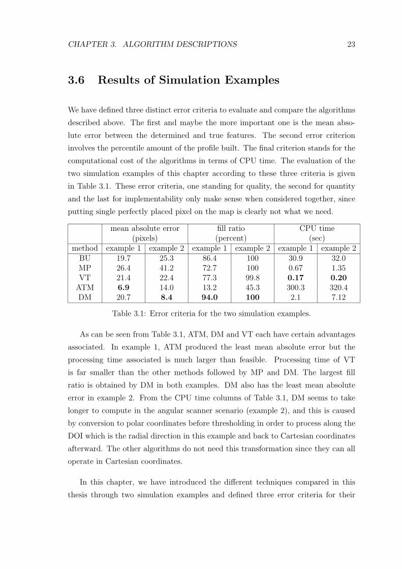
3.6 Results of Simulation Examples
We have defined three distinct error criteria to evaluate and compare the algorithms
described above. The first and maybe the more important one is the mean abso-
lute error between the determined and true features. The second error criterion
involves the percentile amount of the profile built. The final criterion stands for the
computational cost of the algorithms in terms of CPU time. The evaluation of the
two simulation examples of this chapter according to these three criteria is given
in Table 3.1. These error criteria, one standing for quality, the second for quantity
and the last for implementability only make sense when considered together, since
putting single perfectly placed pixel on the map is clearly not what we need.
mean absolute error fill ratio CPU time(pixels) (percent) (sec)
method example 1 example 2 example 1 example 2 example 1 example 2BU 19.7 25.3 86.4 100 30.9 32.0MP 26.4 41.2 72.7 100 0.67 1.35VT 21.4 22.4 77.3 99.8 0.17 0.20
ATM 6.9 14.0 13.2 45.3 300.3 320.4DM 20.7 8.4 94.0 100 2.1 7.12
Table 3.1: Error criteria for the two simulation examples.
As can be seen from Table 3.1, ATM, DM and VT each have certain advantages
associated. In example 1, ATM produced the least mean absolute error but the
processing time associated is much larger than feasible. Processing time of VT
is far smaller than the other methods followed by MP and DM. The largest fill
ratio is obtained by DM in both examples. DM also has the least mean absolute
error in example 2. From the CPU time columns of Table 3.1, DM seems to take
longer to compute in the angular scanner scenario (example 2), and this is caused
by conversion to polar coordinates before thresholding in order to process along the
DOI which is the radial direction in this example and back to Cartesian coordinates
afterward. The other algorithms do not need this transformation since they can all
operate in Cartesian coordinates.
In this chapter, we have introduced the different techniques compared in this
thesis through two simulation examples and defined three error criteria for their

CHAPTER 3. ALGORITHM DESCRIPTIONS 24
comparison. In the following chapter, the same techniques will be compared in
indoor environments using two different approaches for motion planning.
Chapter 4
Indoor Mapping Simulations
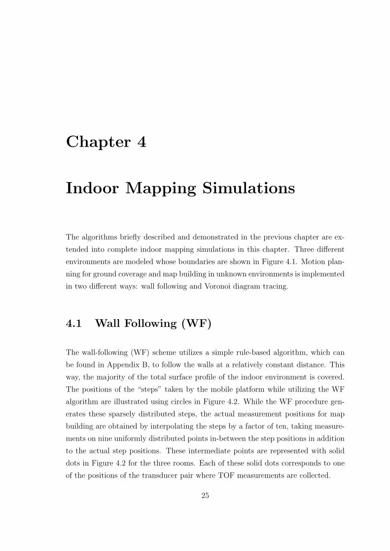
The algorithms briefly described and demonstrated in the previous chapter are ex-
tended into complete indoor mapping simulations in this chapter. Three different
environments are modeled whose boundaries are shown in Figure 4.1. Motion plan-
ning for ground coverage and map building in unknown environments is implemented
in two different ways: wall following and Voronoi diagram tracing.
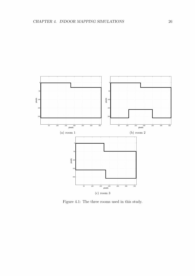
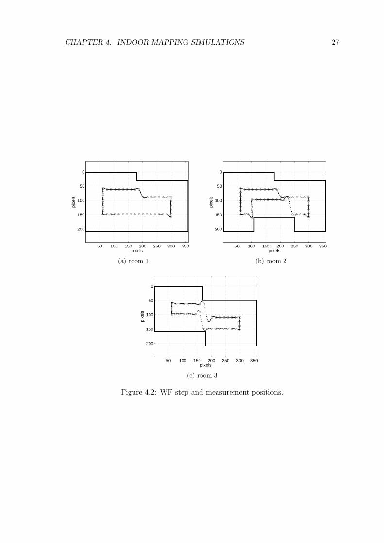
4.1 Wall Following (WF)
The wall-following (WF) scheme utilizes a simple rule-based algorithm, which can
be found in Appendix B, to follow the walls at a relatively constant distance. This
way, the majority of the total surface profile of the indoor environment is covered.
The positions of the “steps” taken by the mobile platform while utilizing the WF
algorithm are illustrated using circles in Figure 4.2. While the WF procedure gen-
erates these sparsely distributed steps, the actual measurement positions for map
building are obtained by interpolating the steps by a factor of ten, taking measure-
ments on nine uniformly distributed points in-between the step positions in addition
to the actual step positions. These intermediate points are represented with solid
dots in Figure 4.2 for the three rooms. Each of these solid dots corresponds to one
of the positions of the transducer pair where TOF measurements are collected.
25
CHAPTER 4. INDOOR MAPPING SIMULATIONS 26
pixels
pixe
ls
50 100 150 200 250 300 350
0
50
100
150
200
(a) room 1
pixels
pixe
ls
50 100 150 200 250 300 350
0
50
100
150
200
(b) room 2
pixels
pixe
ls
50 100 150 200 250 300 350
0
50
100
150
200
(c) room 3
Figure 4.1: The three rooms used in this study.
CHAPTER 4. INDOOR MAPPING SIMULATIONS 27
pixels
pixe
ls
50 100 150 200 250 300 350
0
50
100
150
200
(a) room 1
pixels
pixe
ls
50 100 150 200 250 300 350
0
50
100
150
200
(b) room 2
pixels
pixe
ls
50 100 150 200 250 300 350
0
50
100
150
200
(c) room 3
Figure 4.2: WF step and measurement positions.
CHAPTER 4. INDOOR MAPPING SIMULATIONS 28
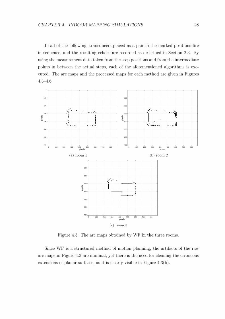
In all of the following, transducers placed as a pair in the marked positions fire
in sequence, and the resulting echoes are recorded as described in Section 2.3. By
using the measurement data taken from the step positions and from the intermediate
points in between the actual steps, each of the aforementioned algorithms is exe-
cuted. The arc maps and the processed maps for each method are given in Figures
4.3–4.6.
pixels
pixe
ls
0 100 200 300 400 500 600 700 800
100
200
300
400
500
600
700
(a) room 1
pixels
pixe
ls
0 100 200 300 400 500 600 700 800
100
200
300
400
500
600
700
(b) room 2
pixels
pixe
ls
0 100 200 300 400 500 600 700 800
100
200
300
400
500
600
700
(c) room 3
Figure 4.3: The arc maps obtained by WF in the three rooms.
Since WF is a structured method of motion planning, the artifacts of the raw
arc maps in Figure 4.3 are minimal, yet there is the need for cleaning the erroneous
extensions of planar surfaces, as it is clearly visible in Figure 4.3(b).
CHAPTER 4. INDOOR MAPPING SIMULATIONS 29
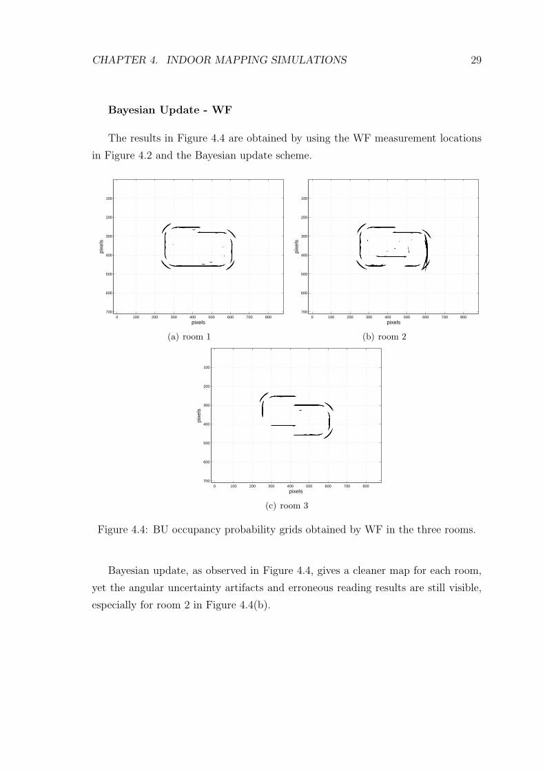
Bayesian Update - WF
The results in Figure 4.4 are obtained by using the WF measurement locations
in Figure 4.2 and the Bayesian update scheme.
pixels
pixe
ls
0 100 200 300 400 500 600 700 800
100
200
300
400
500
600
700
(a) room 1
pixels
pixe
ls
0 100 200 300 400 500 600 700 800
100
200
300
400
500
600
700
(b) room 2
pixels
pixe
ls
0 100 200 300 400 500 600 700 800
100
200
300
400
500
600
700
(c) room 3
Figure 4.4: BU occupancy probability grids obtained by WF in the three rooms.
Bayesian update, as observed in Figure 4.4, gives a cleaner map for each room,
yet the angular uncertainty artifacts and erroneous reading results are still visible,
especially for room 2 in Figure 4.4(b).
CHAPTER 4. INDOOR MAPPING SIMULATIONS 30
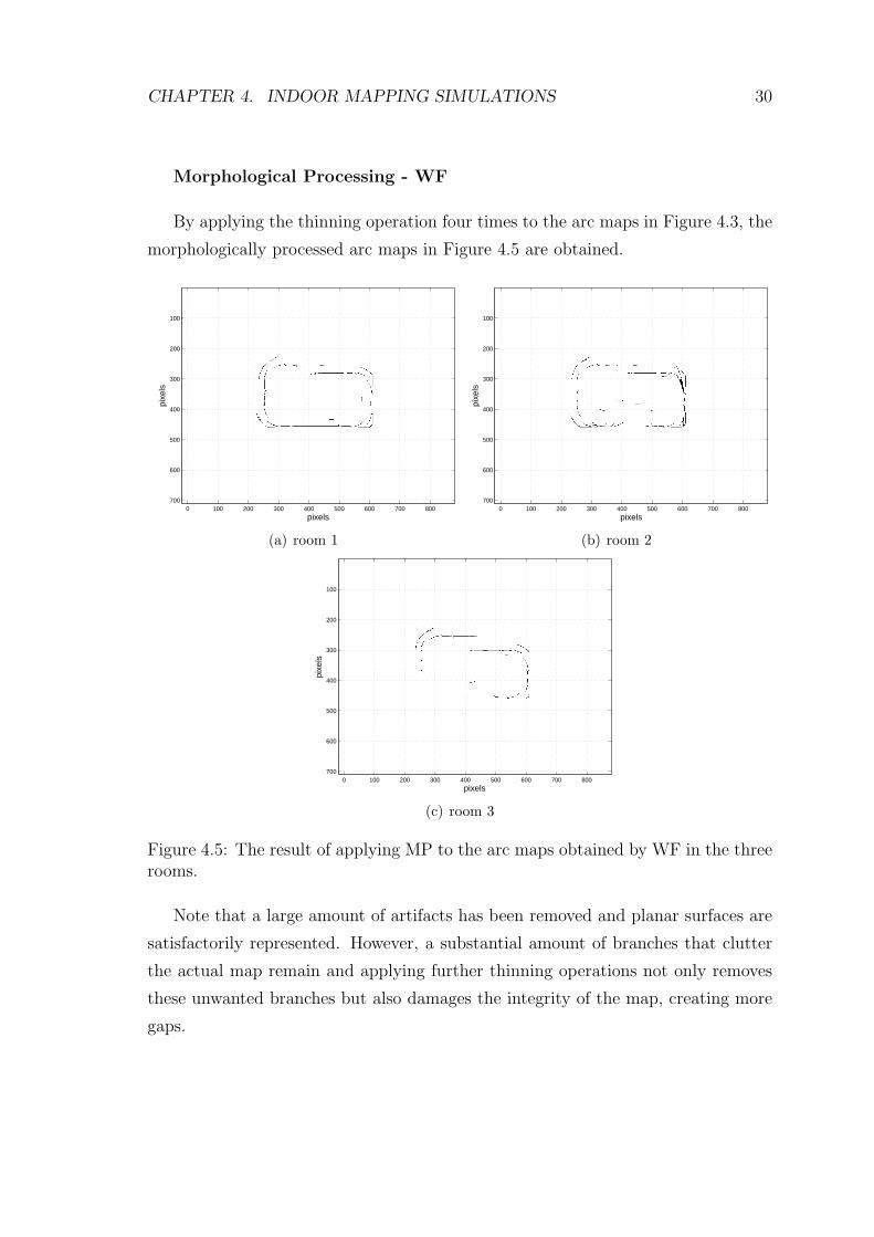
Morphological Processing - WF
By applying the thinning operation four times to the arc maps in Figure 4.3, the
morphologically processed arc maps in Figure 4.5 are obtained.
pixels
pixe
ls
0 100 200 300 400 500 600 700 800
100
200
300
400
500
600
700
(a) room 1
pixels
pixe
ls
0 100 200 300 400 500 600 700 800
100
200
300
400
500
600
700
(b) room 2
pixels
pixe
ls
0 100 200 300 400 500 600 700 800
100
200
300
400
500
600
700
(c) room 3
Figure 4.5: The result of applying MP to the arc maps obtained by WF in the threerooms.
Note that a large amount of artifacts has been removed and planar surfaces are
satisfactorily represented. However, a substantial amount of branches that clutter
the actual map remain and applying further thinning operations not only removes
these unwanted branches but also damages the integrity of the map, creating more
gaps.
CHAPTER 4. INDOOR MAPPING SIMULATIONS 31
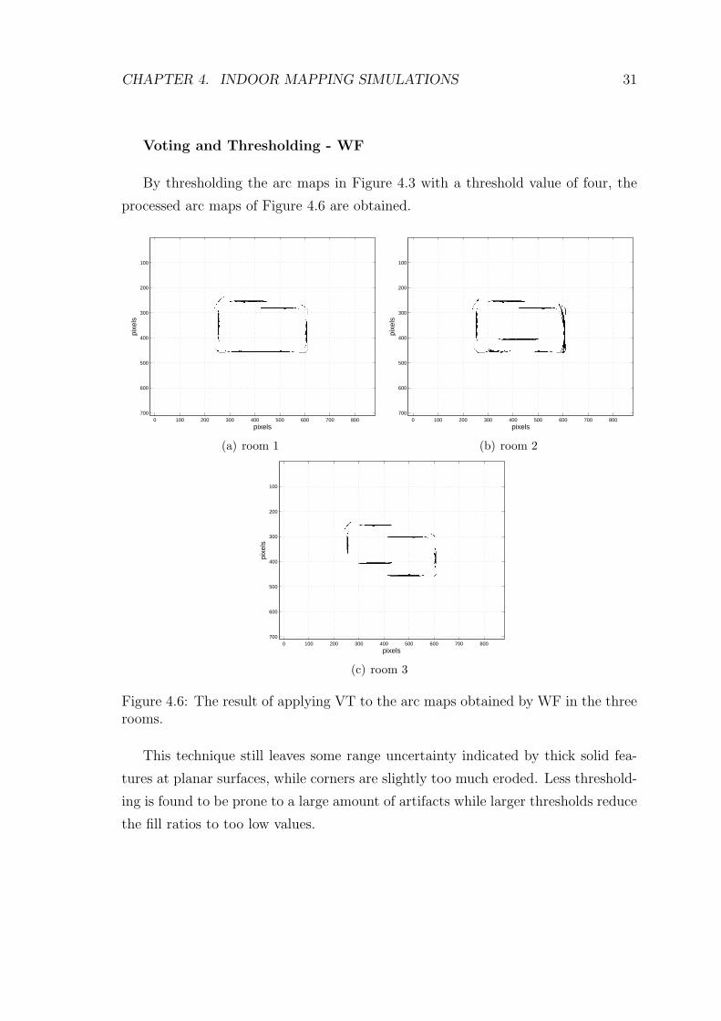
Voting and Thresholding - WF
By thresholding the arc maps in Figure 4.3 with a threshold value of four, the
processed arc maps of Figure 4.6 are obtained.
pixels
pixe
ls
0 100 200 300 400 500 600 700 800
100
200
300
400
500
600
700
(a) room 1
pixels
pixe
ls
0 100 200 300 400 500 600 700 800
100
200
300
400
500
600
700
(b) room 2
pixels
pixe
ls
0 100 200 300 400 500 600 700 800
100
200
300
400
500
600
700
(c) room 3
Figure 4.6: The result of applying VT to the arc maps obtained by WF in the threerooms.
This technique still leaves some range uncertainty indicated by thick solid fea-
tures at planar surfaces, while corners are slightly too much eroded. Less threshold-
ing is found to be prone to a large amount of artifacts while larger thresholds reduce
the fill ratios to too low values.
CHAPTER 4. INDOOR MAPPING SIMULATIONS 32
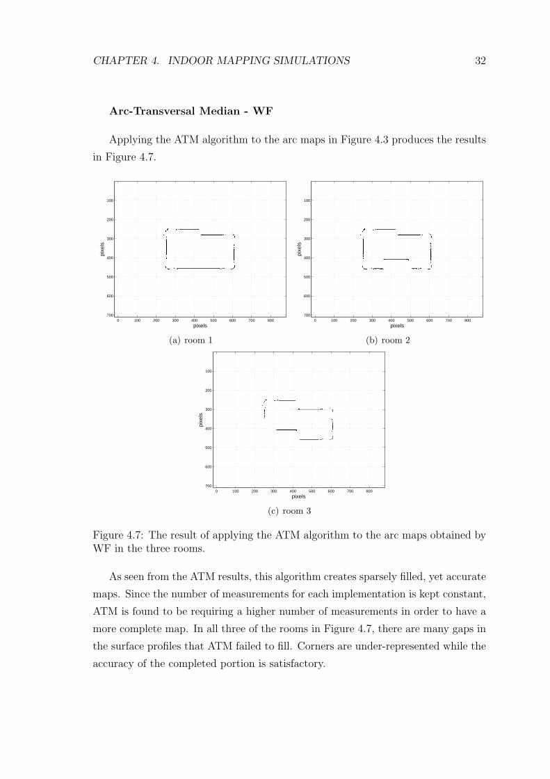
Arc-Transversal Median - WF
Applying the ATM algorithm to the arc maps in Figure 4.3 produces the results
in Figure 4.7.
pixels
pixe
ls
0 100 200 300 400 500 600 700 800
100
200
300
400
500
600
700
(a) room 1
pixels
pixe
ls
0 100 200 300 400 500 600 700 800
100
200
300
400
500
600
700
(b) room 2
pixels
pixe
ls
0 100 200 300 400 500 600 700 800
100
200
300
400
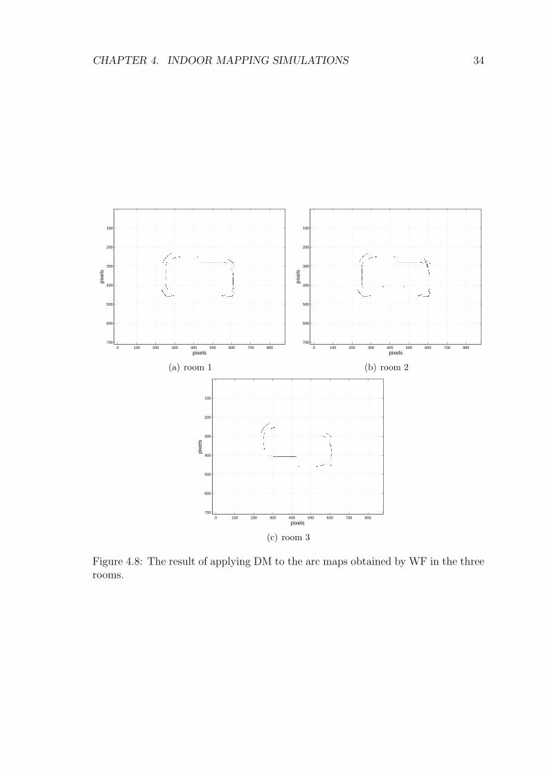
500
600
700
(c) room 3
Figure 4.7: The result of applying the ATM algorithm to the arc maps obtained byWF in the three rooms.
As seen from the ATM results, this algorithm creates sparsely filled, yet accurate
maps. Since the number of measurements for each implementation is kept constant,
ATM is found to be requiring a higher number of measurements in order to have a
more complete map. In all three of the rooms in Figure 4.7, there are many gaps in
the surface profiles that ATM failed to fill. Corners are under-represented while the
accuracy of the completed portion is satisfactory.
CHAPTER 4. INDOOR MAPPING SIMULATIONS 33
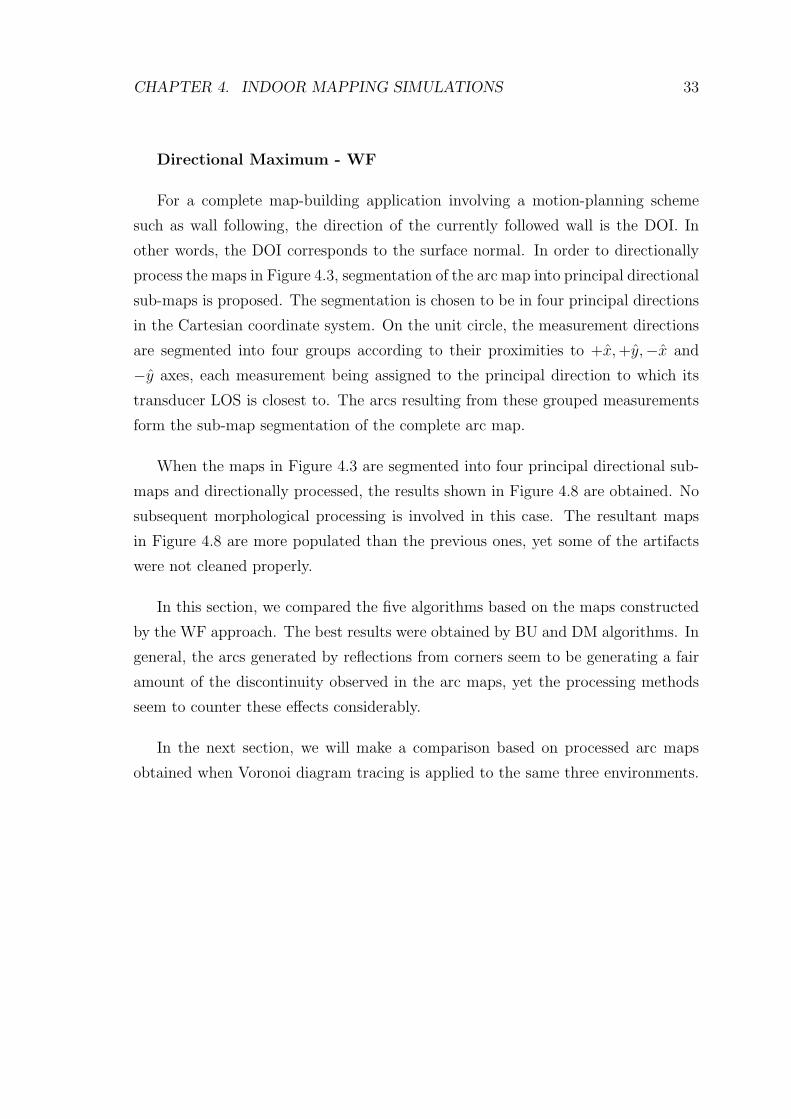
Directional Maximum - WF
For a complete map-building application involving a motion-planning scheme
such as wall following, the direction of the currently followed wall is the DOI. In
other words, the DOI corresponds to the surface normal. In order to directionally
process the maps in Figure 4.3, segmentation of the arc map into principal directional
sub-maps is proposed. The segmentation is chosen to be in four principal directions
in the Cartesian coordinate system. On the unit circle, the measurement directions
are segmented into four groups according to their proximities to +x, +y,−x and
−y axes, each measurement being assigned to the principal direction to which its
transducer LOS is closest to. The arcs resulting from these grouped measurements
form the sub-map segmentation of the complete arc map.
When the maps in Figure 4.3 are segmented into four principal directional sub-
maps and directionally processed, the results shown in Figure 4.8 are obtained. No
subsequent morphological processing is involved in this case. The resultant maps
in Figure 4.8 are more populated than the previous ones, yet some of the artifacts
were not cleaned properly.
In this section, we compared the five algorithms based on the maps constructed
by the WF approach. The best results were obtained by BU and DM algorithms. In
general, the arcs generated by reflections from corners seem to be generating a fair
amount of the discontinuity observed in the arc maps, yet the processing methods
seem to counter these effects considerably.
In the next section, we will make a comparison based on processed arc maps
obtained when Voronoi diagram tracing is applied to the same three environments.
CHAPTER 4. INDOOR MAPPING SIMULATIONS 34
pixels
pixe
ls
0 100 200 300 400 500 600 700 800
100
200
300
400
500
600
700
(a) room 1
pixels
pixe
ls
0 100 200 300 400 500 600 700 800
100
200
300
400
500
600
700
(b) room 2
pixels
pixe
ls
0 100 200 300 400 500 600 700 800
100
200
300
400
500
600
700
(c) room 3
Figure 4.8: The result of applying DM to the arc maps obtained by WF in the threerooms.
CHAPTER 4. INDOOR MAPPING SIMULATIONS 35
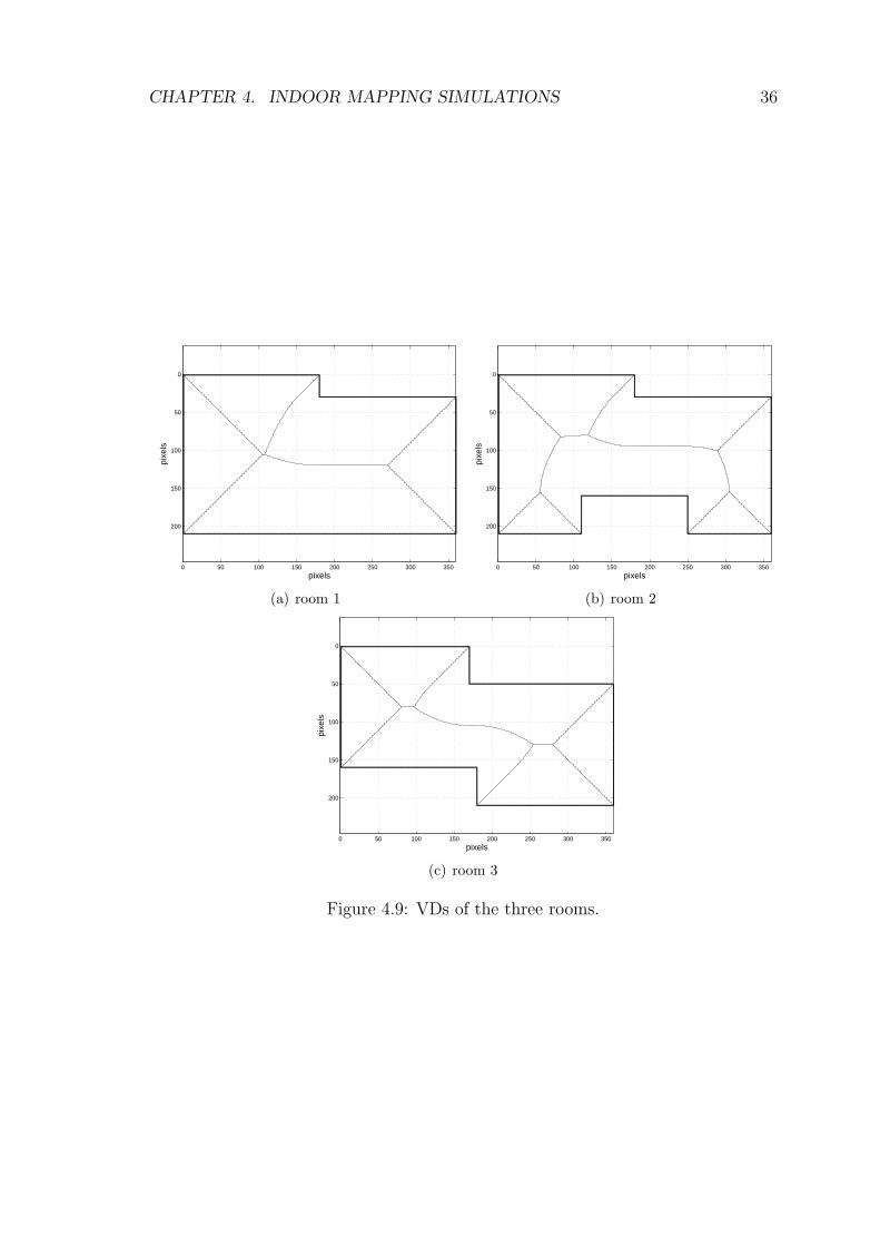
4.2 Voronoi Diagram (VD) Tracing
On a 2-D map containing objects or obstacles, Voronoi diagram (VD) is a tool that
can be used to obtain proximity information. When each point on the 2-D plane
is assigned to the nearest obstacle/object, a number of points are bound to be left
unassigned since they are equidistant to more than one point. These points, which
are on equidistant lines to obstacles/objects form the VD. By constructing the VD
of the unknown environment iteratively as described in [25, 26], and tracing the
respective VD, structured motion planning can be achieved.
Although there exists iterative methods of VD construction for mobile robots
that utilize the gradient-ascent operation to the minimum distance of a point to the
set of all obstacles in the environment [25, 26], we employed a simpler approach for
simulation purposes. The VDs utilized in our simulations are calculated with the
knowledge of the room map in question. This way, the resultant VDs are ideal while
iterative methodology requires high-level control rules to keep the robot close to the
actual VD edges. One can employ the iterative approach in the real-life scenario,
but the ideal VD is far better suited to our needs since the main scope of this thesis
is not the motion-planning part of the application.
The VDs shown in Figure 4.9 are obtained from our room models given in Fig-
ure 4.1.
CHAPTER 4. INDOOR MAPPING SIMULATIONS 36
0 50 100 150 200 250 300 350
0
50
100
150
200
pixels
pixe
ls
(a) room 1
0 50 100 150 200 250 300 350
0
50
100
150
200
pixels
pixe
ls
(b) room 2
0 50 100 150 200 250 300 350
0
50
100
150
200
pixels
pixe
ls
(c) room 3
Figure 4.9: VDs of the three rooms.
CHAPTER 4. INDOOR MAPPING SIMULATIONS 37
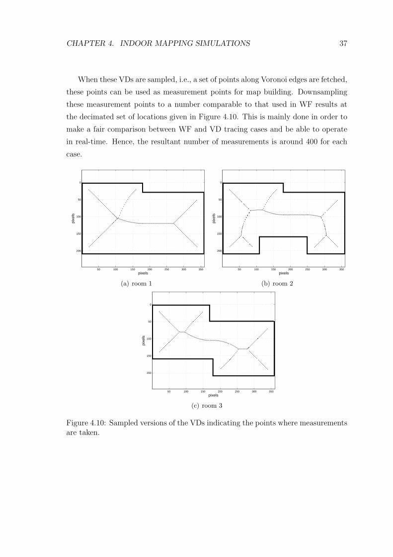
When these VDs are sampled, i.e., a set of points along Voronoi edges are fetched,
these points can be used as measurement points for map building. Downsampling
these measurement points to a number comparable to that used in WF results at
the decimated set of locations given in Figure 4.10. This is mainly done in order to
make a fair comparison between WF and VD tracing cases and be able to operate
in real-time. Hence, the resultant number of measurements is around 400 for each
case.
pixels
pixe
ls
50 100 150 200 250 300 350
0
50
100
150
200
(a) room 1
pixels
pixe
ls
50 100 150 200 250 300 350
0
50
100
150
200
(b) room 2
pixels
pixe
ls
50 100 150 200 250 300 350
0
50
100
150
200
(c) room 3
Figure 4.10: Sampled versions of the VDs indicating the points where measurementsare taken.
CHAPTER 4. INDOOR MAPPING SIMULATIONS 38
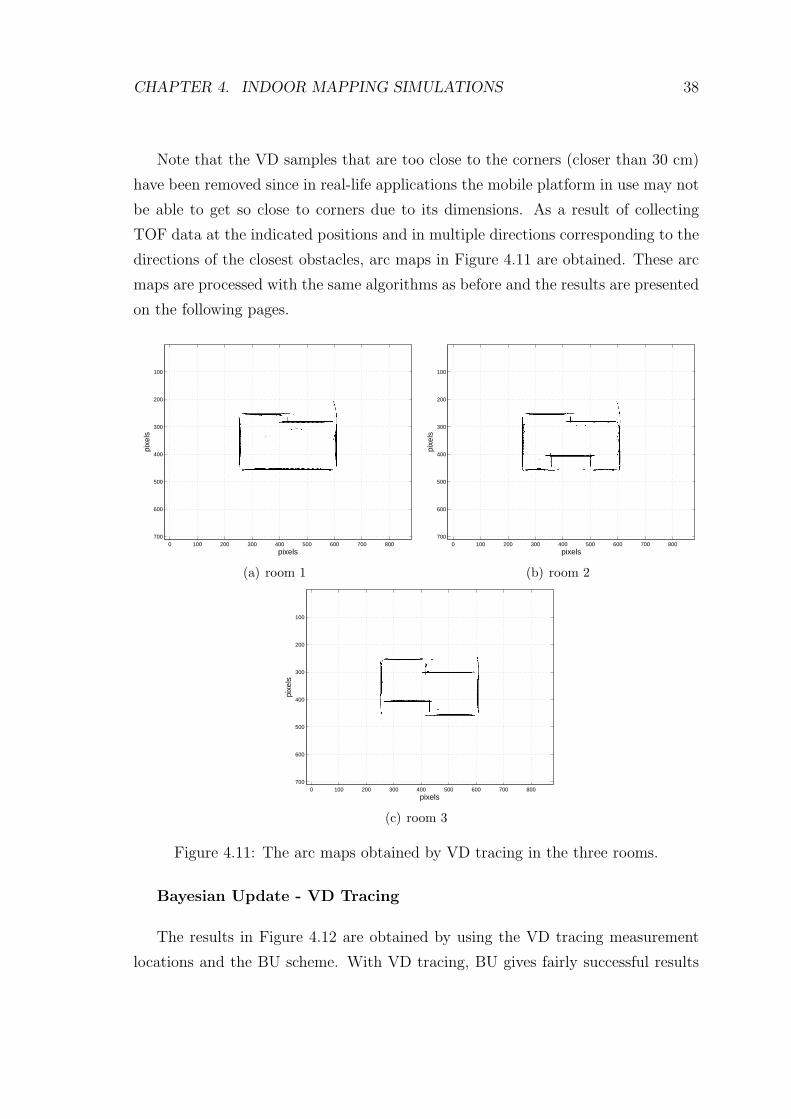
Note that the VD samples that are too close to the corners (closer than 30 cm)
have been removed since in real-life applications the mobile platform in use may not
be able to get so close to corners due to its dimensions. As a result of collecting
TOF data at the indicated positions and in multiple directions corresponding to the
directions of the closest obstacles, arc maps in Figure 4.11 are obtained. These arc
maps are processed with the same algorithms as before and the results are presented
on the following pages.
pixels
pixe
ls
0 100 200 300 400 500 600 700 800
100
200
300
400
500
600
700
(a) room 1
pixels
pixe
ls
0 100 200 300 400 500 600 700 800
100
200
300
400
500
600
700
(b) room 2
pixels
pixe
ls
0 100 200 300 400 500 600 700 800
100
200
300
400
500
600
700
(c) room 3
Figure 4.11: The arc maps obtained by VD tracing in the three rooms.
Bayesian Update - VD Tracing
The results in Figure 4.12 are obtained by using the VD tracing measurement
locations and the BU scheme. With VD tracing, BU gives fairly successful results
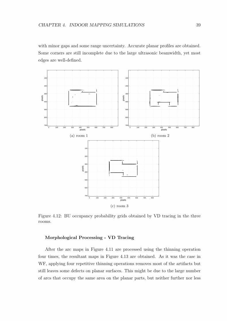
CHAPTER 4. INDOOR MAPPING SIMULATIONS 39
with minor gaps and some range uncertainty. Accurate planar profiles are obtained.
Some corners are still incomplete due to the large ultrasonic beamwidth, yet most
edges are well-defined.
pixels
pixe
ls
0 100 200 300 400 500 600 700 800
100
200
300
400
500
600
700
(a) room 1
pixels
pixe
ls
0 100 200 300 400 500 600 700 800
100
200
300
400
500
600
700
(b) room 2
pixels
pixe
ls
0 100 200 300 400 500 600 700 800
100
200
300
400
500
600
700
(c) room 3
Figure 4.12: BU occupancy probability grids obtained by VD tracing in the threerooms.
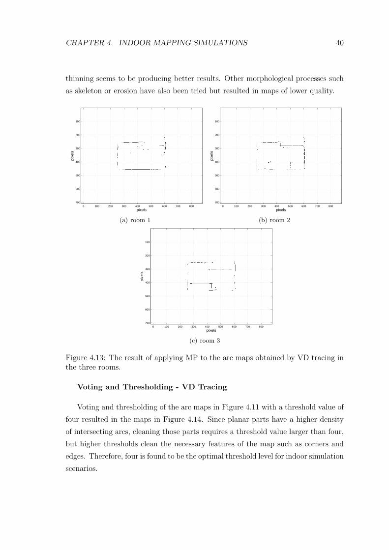
Morphological Processing - VD Tracing
After the arc maps in Figure 4.11 are processed using the thinning operation
four times, the resultant maps in Figure 4.13 are obtained. As it was the case in
WF, applying four repetitive thinning operations removes most of the artifacts but
still leaves some defects on planar surfaces. This might be due to the large number
of arcs that occupy the same area on the planar parts, but neither further nor less
CHAPTER 4. INDOOR MAPPING SIMULATIONS 40
thinning seems to be producing better results. Other morphological processes such
as skeleton or erosion have also been tried but resulted in maps of lower quality.
pixels
pixe
ls
0 100 200 300 400 500 600 700 800
100
200
300
400
500
600
700
(a) room 1
pixelspi
xels
0 100 200 300 400 500 600 700 800
100
200
300
400
500
600
700
(b) room 2
pixels
pixe
ls
0 100 200 300 400 500 600 700 800
100
200
300
400
500
600
700
(c) room 3
Figure 4.13: The result of applying MP to the arc maps obtained by VD tracing inthe three rooms.
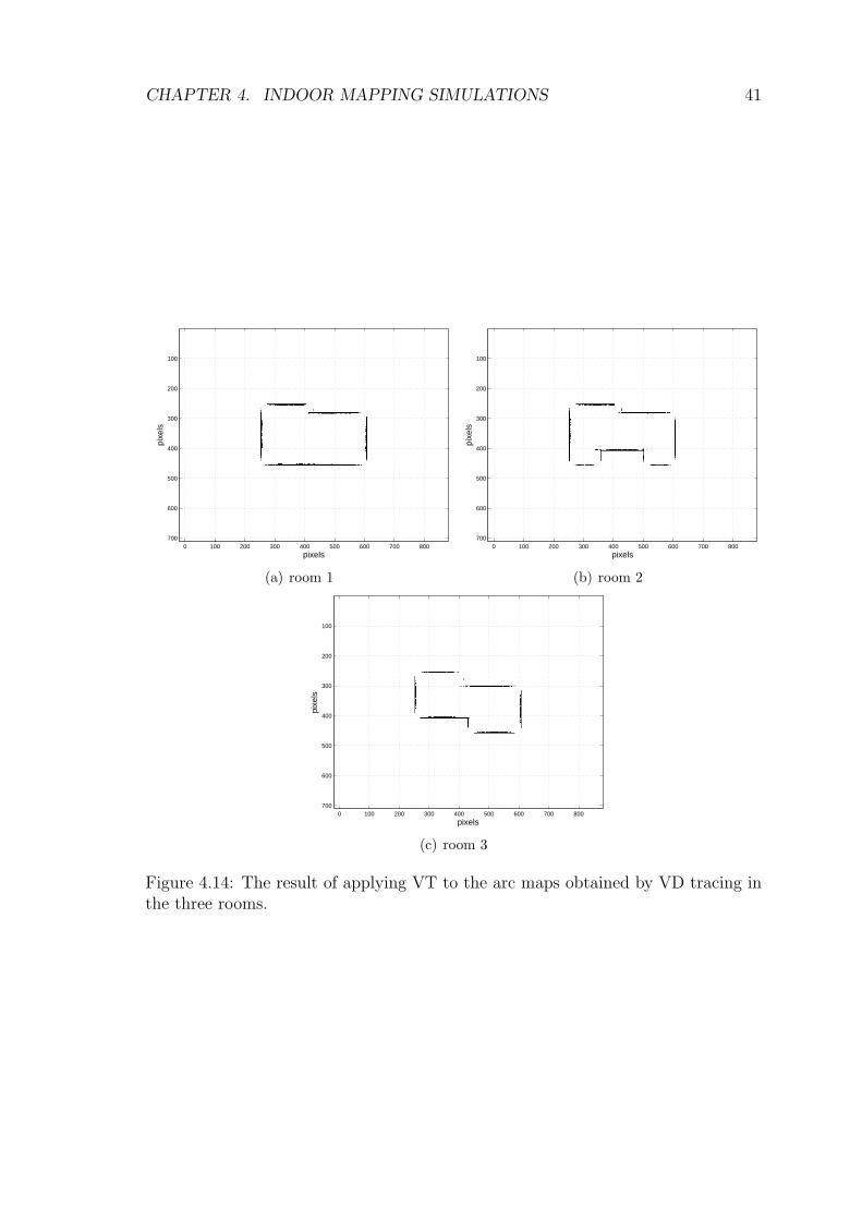
Voting and Thresholding - VD Tracing
Voting and thresholding of the arc maps in Figure 4.11 with a threshold value of
four resulted in the maps in Figure 4.14. Since planar parts have a higher density
of intersecting arcs, cleaning those parts requires a threshold value larger than four,
but higher thresholds clean the necessary features of the map such as corners and
edges. Therefore, four is found to be the optimal threshold level for indoor simulation
scenarios.
CHAPTER 4. INDOOR MAPPING SIMULATIONS 41
pixels
pixe
ls
0 100 200 300 400 500 600 700 800
100
200
300
400
500
600
700
(a) room 1
pixels
pixe
ls
0 100 200 300 400 500 600 700 800
100
200
300
400
500
600
700
(b) room 2
pixels
pixe
ls
0 100 200 300 400 500 600 700 800
100
200
300
400
500
600
700
(c) room 3
Figure 4.14: The result of applying VT to the arc maps obtained by VD tracing inthe three rooms.
CHAPTER 4. INDOOR MAPPING SIMULATIONS 42
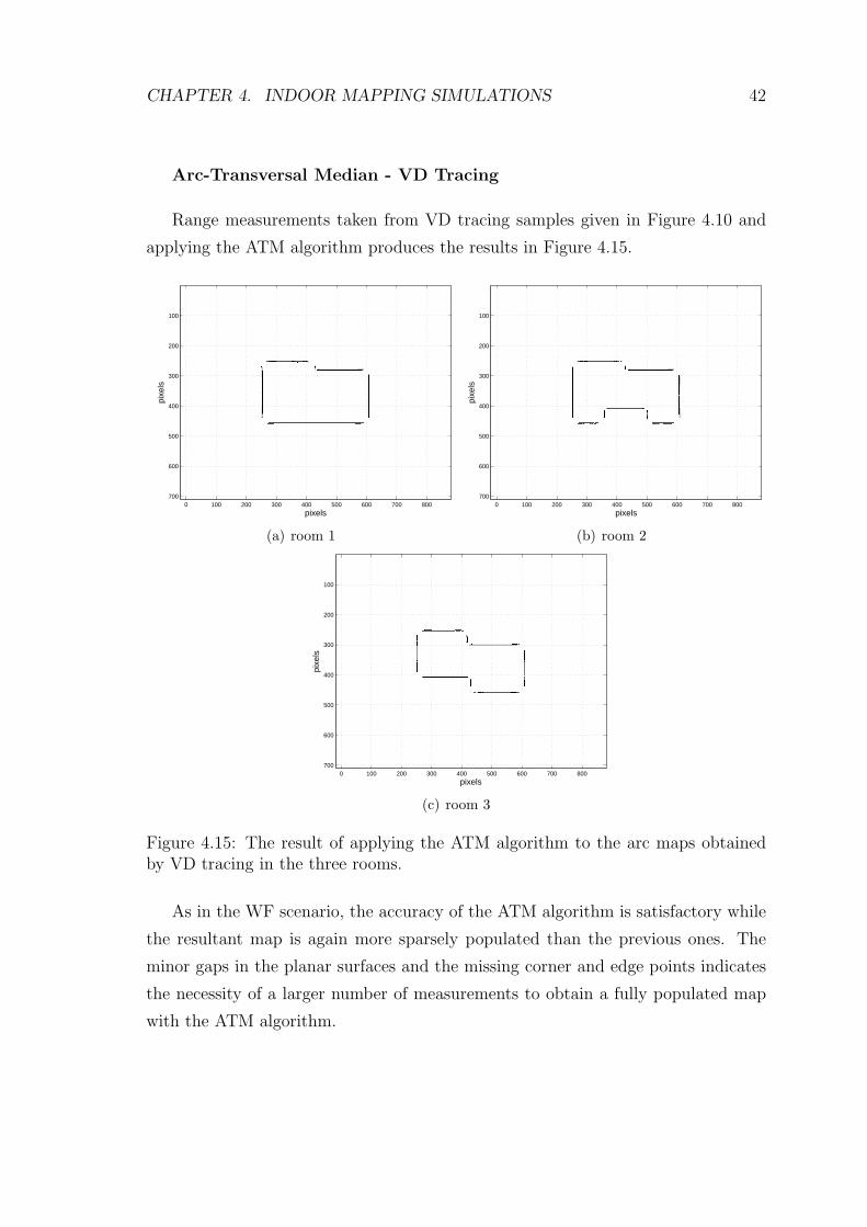
Arc-Transversal Median - VD Tracing
Range measurements taken from VD tracing samples given in Figure 4.10 and
applying the ATM algorithm produces the results in Figure 4.15.
pixels
pixe
ls
0 100 200 300 400 500 600 700 800
100
200
300
400
500
600
700
(a) room 1
pixels
pixe
ls
0 100 200 300 400 500 600 700 800
100
200
300
400
500
600
700
(b) room 2
pixels
pixe
ls
0 100 200 300 400 500 600 700 800
100
200
300
400
500
600
700
(c) room 3
Figure 4.15: The result of applying the ATM algorithm to the arc maps obtainedby VD tracing in the three rooms.
As in the WF scenario, the accuracy of the ATM algorithm is satisfactory while
the resultant map is again more sparsely populated than the previous ones. The
minor gaps in the planar surfaces and the missing corner and edge points indicates
the necessity of a larger number of measurements to obtain a fully populated map
with the ATM algorithm.
CHAPTER 4. INDOOR MAPPING SIMULATIONS 43
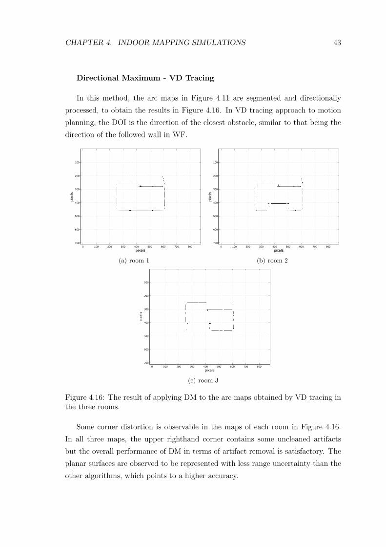
Directional Maximum - VD Tracing
In this method, the arc maps in Figure 4.11 are segmented and directionally
processed, to obtain the results in Figure 4.16. In VD tracing approach to motion
planning, the DOI is the direction of the closest obstacle, similar to that being the
direction of the followed wall in WF.
pixels
pixe
ls
0 100 200 300 400 500 600 700 800
100
200
300
400
500
600
700
(a) room 1
pixels
pixe
ls
0 100 200 300 400 500 600 700 800
100
200
300
400
500
600
700
(b) room 2
pixels
pixe
ls
0 100 200 300 400 500 600 700 800
100
200
300
400
500
600
700
(c) room 3
Figure 4.16: The result of applying DM to the arc maps obtained by VD tracing inthe three rooms.
Some corner distortion is observable in the maps of each room in Figure 4.16.
In all three maps, the upper righthand corner contains some uncleaned artifacts
but the overall performance of DM in terms of artifact removal is satisfactory. The
planar surfaces are observed to be represented with less range uncertainty than the
other algorithms, which points to a higher accuracy.
CHAPTER 4. INDOOR MAPPING SIMULATIONS 44
4.3 Results of Indoor Mapping Simulations
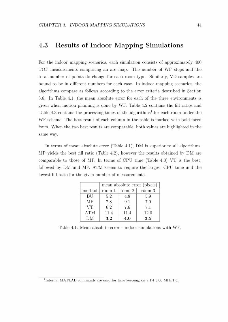
For the indoor mapping scenarios, each simulation consists of approximately 400
TOF measurements comprising an arc map. The number of WF steps and the
total number of points do change for each room type. Similarly, VD samples are
bound to be in different numbers for each case. In indoor mapping scenarios, the
algorithms compare as follows according to the error criteria described in Section
3.6. In Table 4.1, the mean absolute error for each of the three environments is
given when motion planning is done by WF. Table 4.2 contains the fill ratios and
Table 4.3 contains the processing times of the algorithms1 for each room under the
WF scheme. The best result of each column in the table is marked with bold faced
fonts. When the two best results are comparable, both values are highlighted in the
same way.
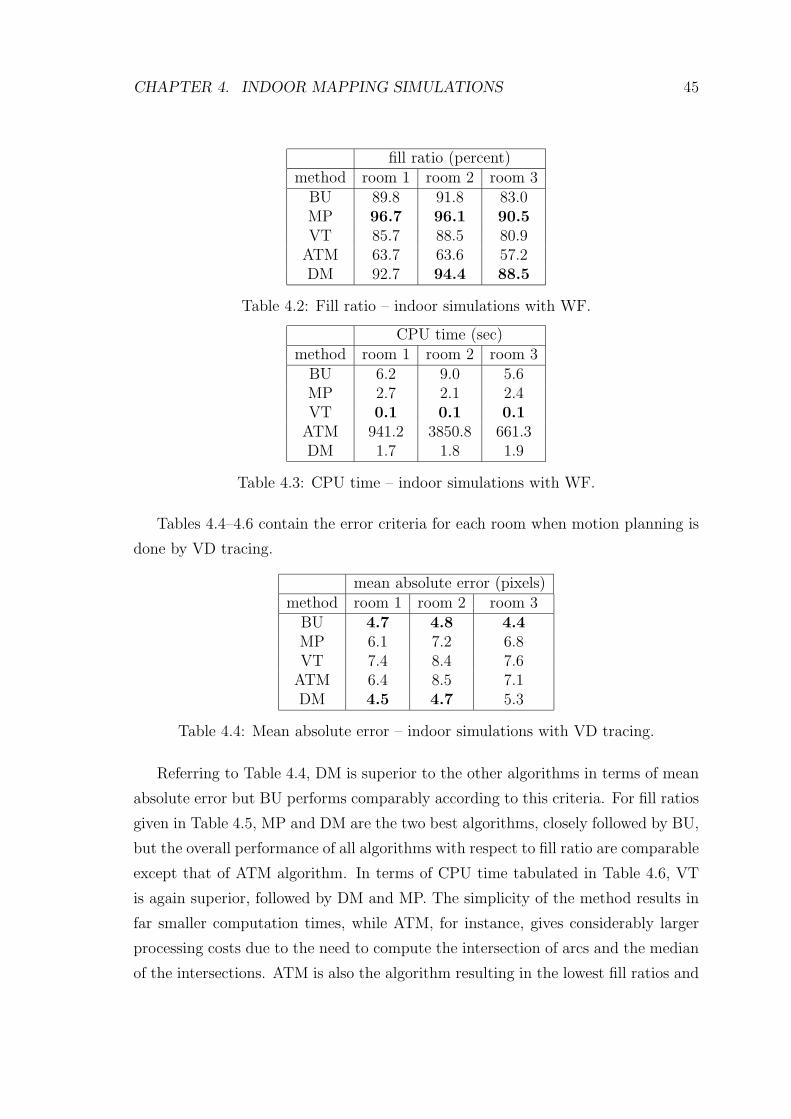
In terms of mean absolute error (Table 4.1), DM is superior to all algorithms.
MP yields the best fill ratio (Table 4.2), however the results obtained by DM are
comparable to those of MP. In terms of CPU time (Table 4.3) VT is the best,
followed by DM and MP. ATM seems to require the largest CPU time and the
lowest fill ratio for the given number of measurements.
mean absolute error (pixels)method room 1 room 2 room 3
BU 5.2 4.8 5.9MP 7.8 9.1 7.0VT 6.2 7.6 7.1
ATM 11.4 11.4 12.0DM 3.2 4.0 3.5
Table 4.1: Mean absolute error – indoor simulations with WF.
1Internal MATLAB commands are used for time keeping, on a P4 3.06 MHz PC.
CHAPTER 4. INDOOR MAPPING SIMULATIONS 45
fill ratio (percent)method room 1 room 2 room 3
BU 89.8 91.8 83.0MP 96.7 96.1 90.5VT 85.7 88.5 80.9
ATM 63.7 63.6 57.2DM 92.7 94.4 88.5
Table 4.2: Fill ratio – indoor simulations with WF.
CPU time (sec)method room 1 room 2 room 3
BU 6.2 9.0 5.6MP 2.7 2.1 2.4VT 0.1 0.1 0.1
ATM 941.2 3850.8 661.3DM 1.7 1.8 1.9
Table 4.3: CPU time – indoor simulations with WF.
Tables 4.4–4.6 contain the error criteria for each room when motion planning is
done by VD tracing.
mean absolute error (pixels)method room 1 room 2 room 3
BU 4.7 4.8 4.4MP 6.1 7.2 6.8VT 7.4 8.4 7.6
ATM 6.4 8.5 7.1DM 4.5 4.7 5.3
Table 4.4: Mean absolute error – indoor simulations with VD tracing.
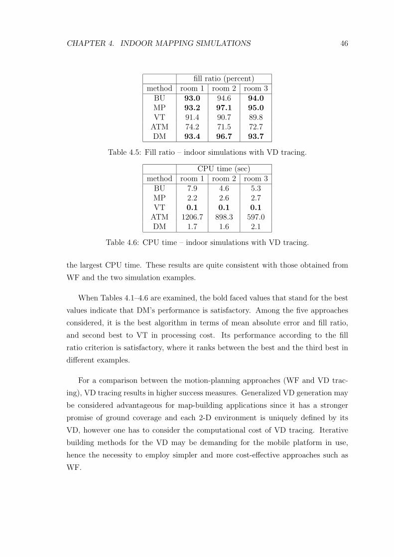
Referring to Table 4.4, DM is superior to the other algorithms in terms of mean
absolute error but BU performs comparably according to this criteria. For fill ratios
given in Table 4.5, MP and DM are the two best algorithms, closely followed by BU,
but the overall performance of all algorithms with respect to fill ratio are comparable
except that of ATM algorithm. In terms of CPU time tabulated in Table 4.6, VT
is again superior, followed by DM and MP. The simplicity of the method results in
far smaller computation times, while ATM, for instance, gives considerably larger
processing costs due to the need to compute the intersection of arcs and the median
of the intersections. ATM is also the algorithm resulting in the lowest fill ratios and
CHAPTER 4. INDOOR MAPPING SIMULATIONS 46
fill ratio (percent)method room 1 room 2 room 3
BU 93.0 94.6 94.0MP 93.2 97.1 95.0VT 91.4 90.7 89.8
ATM 74.2 71.5 72.7DM 93.4 96.7 93.7
Table 4.5: Fill ratio – indoor simulations with VD tracing.
CPU time (sec)method room 1 room 2 room 3
BU 7.9 4.6 5.3MP 2.2 2.6 2.7VT 0.1 0.1 0.1
ATM 1206.7 898.3 597.0DM 1.7 1.6 2.1
Table 4.6: CPU time – indoor simulations with VD tracing.
the largest CPU time. These results are quite consistent with those obtained from
WF and the two simulation examples.
When Tables 4.1–4.6 are examined, the bold faced values that stand for the best
values indicate that DM’s performance is satisfactory. Among the five approaches
considered, it is the best algorithm in terms of mean absolute error and fill ratio,
and second best to VT in processing cost. Its performance according to the fill
ratio criterion is satisfactory, where it ranks between the best and the third best in
different examples.
For a comparison between the motion-planning approaches (WF and VD trac-
ing), VD tracing results in higher success measures. Generalized VD generation may
be considered advantageous for map-building applications since it has a stronger
promise of ground coverage and each 2-D environment is uniquely defined by its
VD, however one has to consider the computational cost of VD tracing. Iterative
building methods for the VD may be demanding for the mobile platform in use,
hence the necessity to employ simpler and more cost-effective approaches such as
WF.

CHAPTER 4. INDOOR MAPPING SIMULATIONS 47
In this chapter, we compared the algorithms for map-building in indoor environ-
ments using two ways of motion planning. In the final chapter we discuss the main
conclusions and future extensions of the work reported here.
Chapter 5
Conclusions
The main contribution of this thesis has been providing a comparison between dif-
ferent algorithms for processing ultrasonic arc maps for map-building purposes. The
results indicate that the newly proposed DM algorithm has some advantages over
the existing algorithms, while among the existing four algorithms each has stronger
or weaker characteristics that might be suitable for certain situations or conditions.
Having the minimum mean absolute error, DM should be considered a good choice
in most cases, while strict requirements on computational cost might lead to the use
of VT algorithm since it requires far smaller CPU time to operate. In addition, MP
might be considered when a rough yet full view of the environment is required as the
computational cost of MP is still achievable in real-time even though the associated
mean absolute errors are not as good as those of DM.
DM in itself has added an important aspect to the map-building algorithms
which is the direction of interest. The sense of direction readily available in most
motion-planning schemes is shown to be an effective addition when incorporated
into the map-building algorithm. The directional awareness of the mobile platform
for the sake of surface or profile extraction was proved to deliver satisfactory maps.
In addition, the compared motion-planning approaches showed that VD tracing
is more successful in ground coverage since it includes a more systematic and com-
plete approach to the entire environment. WF also has its merits as the iterative
48
CHAPTER 5. CONCLUSIONS 49
methods to generate a WF motion-plan is far simpler than that of VD tracing and
in most artificial environments simple rule-based algorithms perform well for WF.
VD tracing seems to be the better choice if the computational cost is of secondary
importance as it might be computationally demanding for complex environments.
As for future extensions, multiple reflections might be included in the simulated
signal model. Iterative methods for VD generation would also be a good capability
for the mobile platform since a priori knowledge of the VD might not be readily
available. A more complex WF algorithm can be included in order to map arbitrarily
curved surfaces that can be encountered in natural environments. For DM, a self-
centered polar processing scheme can be developed where several separate locations
of the mobile platform in the environment might be chosen and used as central
points from which the arc map can be radially processed and then fused. Multiple
maxima along directional array can be handled according to the general curvature
of the arcs intersecting at each pixel. Applying active contour models used in image
processing and known as “snakes” to the resultant maps might improve the fill ratios.
The results might be verified experimentally and the approaches can be extended
to other sensing modalities.

Appendix A
Ultrasonic Signal Models
Figure A.1: Geometry of the problem with the given sensor pair when the target isa plane (adopted from [1]).
The echo models used in this thesis and presented in Chapter 2 are based on [1].
For a planar target and separate transducers working as transmitter and receiver
(transducer a and b), the geometry of reflection is illustrated in Figure A.1. Since
each transducer can be employed both as a transmitter and receiver, a set of four
TOF measurements are obtained when the transducers are fired in sequence. From
the geometry, the TOF measurements for each transmitter and receiver pair are
found as
50
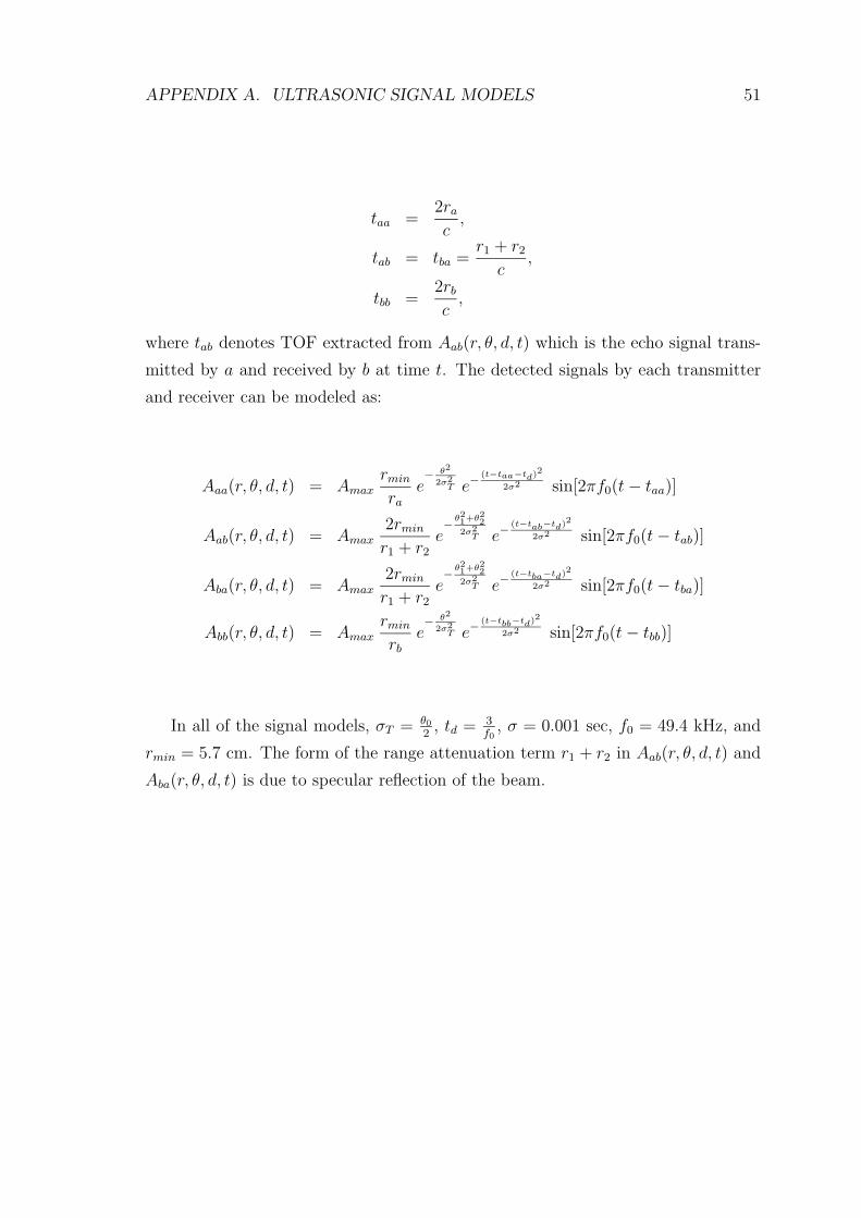
APPENDIX A. ULTRASONIC SIGNAL MODELS 51
taa =2ra
c,
tab = tba =r1 + r2
c,
tbb =2rb
c,
where tab denotes TOF extracted from Aab(r, θ, d, t) which is the echo signal trans-
mitted by a and received by b at time t. The detected signals by each transmitter
and receiver can be modeled as:
Aaa(r, θ, d, t) = Amax
rmin
ra
e−
θ2
2σ2T e−
(t−taa−td)2
2σ2 sin[2πf0(t − taa)]
Aab(r, θ, d, t) = Amax
2rmin
r1 + r2
e−
θ21+θ
22
2σ2T e−
(t−tab−td)2
2σ2 sin[2πf0(t − tab)]
Aba(r, θ, d, t) = Amax
2rmin
r1 + r2
e−
θ21+θ
22
2σ2T e−
(t−tba−td)2
2σ2 sin[2πf0(t − tba)]
Abb(r, θ, d, t) = Amax
rmin
rb
e−
θ2
2σ2T e−
(t−tbb−td)2
2σ2 sin[2πf0(t − tbb)]
In all of the signal models, σT = θ0
2, td = 3
f0, σ = 0.001 sec, f0 = 49.4 kHz, and
rmin = 5.7 cm. The form of the range attenuation term r1 + r2 in Aab(r, θ, d, t) and
Aba(r, θ, d, t) is due to specular reflection of the beam.
Appendix B
Wall-following (WF) Algorithm
The WF algorithm employed in our simulations is a relatively simple and rule-based
approach similar to that described in [46]. If the bearing of the mobile robot is
taken as the reference frame on the 2-D plane, the general intention of the robot is
to keep the wall to be followed on +y direction at all times. This is done as follows:
1. Initialization step: The robot is at an unknown, arbitrary location. Sixteen
range measurements in sixteen directions from the initial point, uniformly dis-
tributed on the unit circle with 22.5◦ intervals are obtained. The minimum
value among these range measurements, which corresponds to the closest ob-
stacle, is taken as the direction of the surface/wall to be followed.
2. First step: The robot approaches to or goes away from the closest surface until
the distance to the surface is 60 cm. Then the robot performs a −90◦ rotation
in order to align the wall to +y direction of its internal frame of reference.
3. Step number 2 to N : Until the robot is in proximity of the initial point (at
20 cm distance to the starting location) or the predetermined number of steps
(an upper limit of 100 steps are chosen) are complete, the robot repeats this
procedure:
Take two range measurements. r1 being the range measured directly ahead or
in +x direction in robot’s reference frame and r2 being the range measured in
52
APPENDIX B. WALL-FOLLOWING (WF) ALGORITHM 53
+y direction in robot’s reference frame, check for the following:
(a) if r2 > 80 cm, then the followed wall is lost. Perform a +90◦ turn and
move 60 cm in three separate steps of 20 cm each.
(b) if r2 ≤ 80 cm and r1 > 60 cm, then take a step ahead. Move 15 cm ahead
and make any additional course correction necessary to keep the distance
to the wall (r2) at 60 cm.
(c) if both r2 ≤ 80 cm and r1 ≤ 60 cm, then perform a −90◦ turn. This
corresponds to the presence of a left-hand corner, so the new wall is
followed after this step.
The above described procedure is found to be simple enough yet effective in most
indoor environments that have artificial surfaces and obstacles, interfacing at right
angles. A flow chart of the algorithm can be found in Figure B.1. The threshold
values for r1 and r2 are set after a number of trials. The result of this algorithm
when applied to the room examples of Figure 4.1 in Chapter 4 are presented in
Figure 4.2.
For more complex environments and/or cases where computational cost of the
algorithm is not an issue, potential-based WF algorithms can also be employed [19–
21].
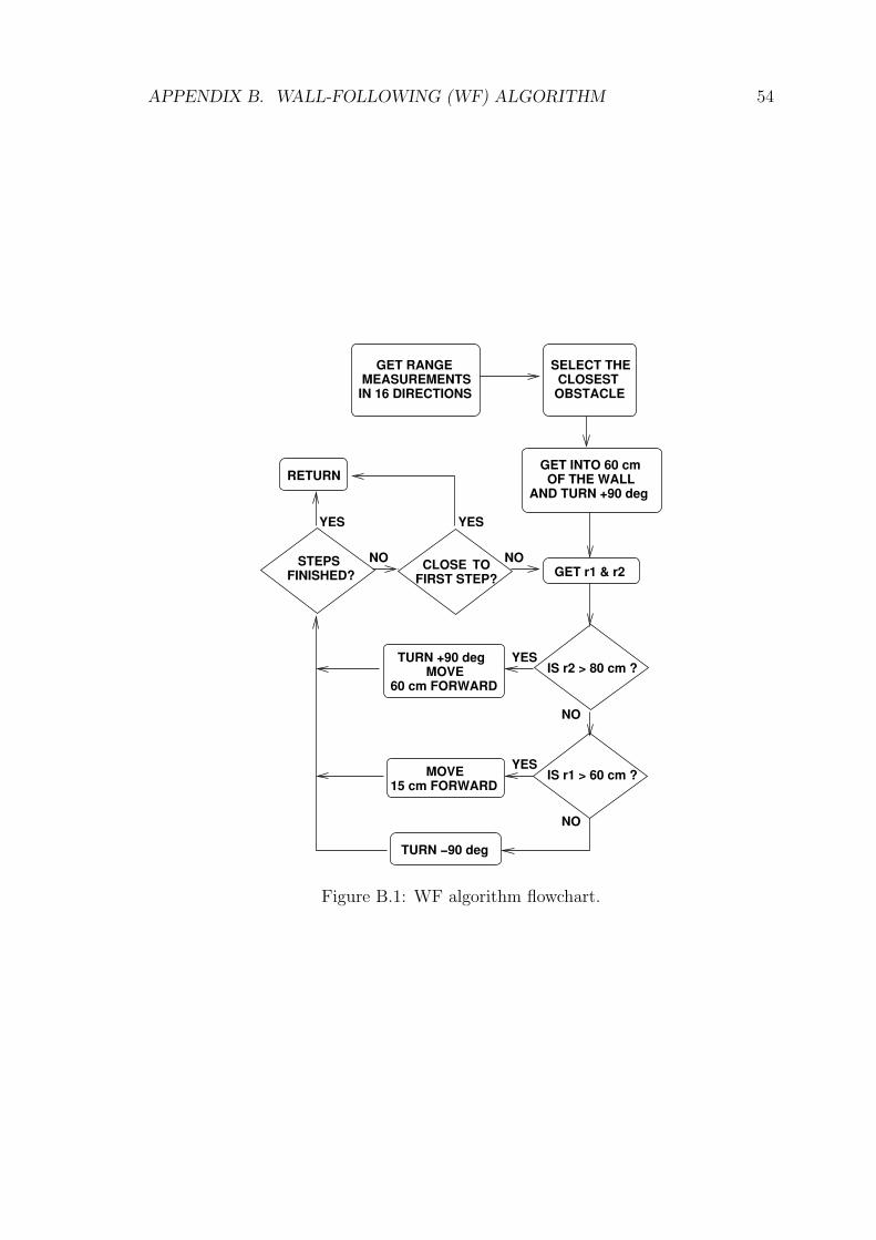
APPENDIX B. WALL-FOLLOWING (WF) ALGORITHM 54
GET RANGEMEASUREMENTSIN 16 DIRECTIONS
SELECT THECLOSESTOBSTACLE
GET INTO 60 cmOF THE WALL
AND TURN +90 deg
GET r1 & r2
IS r2 > 80 cm ?
NO
YES
IS r1 > 60 cm ?YES
NO
MOVE15 cm FORWARD
TURN −90 deg
TURN +90 degMOVE
60 cm FORWARD
FINISHED?STEPS CLOSE
FIRST STEP?TO
RETURN
YESYES
NO NO
Figure B.1: WF algorithm flowchart.
Appendix C
MATLAB Simulation Codes
The MATLAB code used in the simulations can be found on the following pages.
55
C:\MATLAB7\work\appendix.m Page 1
function wall_foll_map(type)
% WALL FOLLOWING TYPE MOTION-PLANNING BASED % MAP BUILDING SCRIPT, UTILIZING MP, VT, ATM & DM % GETS THE PARAMETER type TO INDICATE ROOM TYPE
disp('==========================================') disp(['Wall Following, Room Type ' int2str(type)]) disp('==========================================')
room=draw_room4(type);print('-deps',strcat('room_def_type_',int2str(type))) [Y,X]=size(room);% DEFINE THE ROOM, EXPORT EPS FIGURE OF THE ROOM AND GET SIZE
load(strcat('wall_foll_type_',int2str(type))); % LOAD WALL FOLLOWING STEP LOCATIONS
%=========================% MORPHOLOGICAL PROCESSING %=========================x_array1=wf(1,:);y_array1=wf(2,:);b_array1=wf(3,:)+90;% EXTRACT LOCATIONS AND BEARINGS
x_array=interp(x_array1,10);y_array=interp(y_array1,10);b_array=interp(b_array1,10);% INTERPOLATE STEP POSITIONS TO GET MEASUREMENT LOCATIONS
x_array=fix(x_array);y_array=fix(y_array);b_array=fix(b_array);totalsonarno=length(x_array)% FIX THE PIXELS TO SMALLEST INTEGER AND DISPLAY TOTAL MEASUREMENT POINT #
base_dm=zeros(Y+500,X+500);% ALLOCATE EMPTY ARC-MAP ARRAY FOR BOOK KEEPING
for son=1:length(x_array) base_dm=sonarPut5(x_array(son),y_array(son),b_array(son),room,base_dm); end% PLACE THE SONARS
base=base_dm;% COPY THE ARC MAP TO BE PROCESSED
tic% START KEEPING THE TIME
base2=logical(sign(base));
C:\MATLAB7\work\appendix.m Page 2
% CONVERT ARC MAP TO LOGICAL
base3=bwmorph(base2,'thin',4); % APPLY MORPHOLOGICAL PROCESSING
time_morph=toc% GET THE COMPUTATION TIME
figurecolormap(gray(2))image(2-2*base2)grid on xlabel('pixels','FontSize',14) ylabel('pixels','FontSize',14) axis equal print('-deps',strcat('mp1_wf_type_',int2str(type))) % DISPLAY AND EXPORT BINARY ARC MAP
figurecolormap(gray(2))image(2-2*base3)grid on xlabel('pixels','FontSize',14) ylabel('pixels','FontSize',14) axis equal print('-deps',strcat('mp2_wf_type_',int2str(type))) % DISPLAY AND EXPORT MP ARCS
%========================% VOTING AND THRESHOLDING %========================tic% START KEEPING THE TIME
thres=4;% SET THE THRESHOLD
base4=sign(floor(base/thres));% APPLY THE THRESHOLD
time_vote=toc% GET THE COMPUTATION TIME
figurecolormap(gray(255))scale=255/max(max(base));image(255-scale*base)axis equal grid on xlabel('pixels','FontSize',14) ylabel('pixels','FontSize',14) print('-deps',strcat('vt1_wf_type_',int2str(type)))
C:\MATLAB7\work\appendix.m Page 3
% DISPLAY AND EXPORT INTEGER ARC MAP
figurecolormap(gray(255))image(255-255*base4)grid on xlabel('pixels','FontSize',14) ylabel('pixels','FontSize',14) axis equal print('-deps',strcat('vt2_wf_type_',int2str(type))) % DISPLAY AND EXPORT VT ARC MAP
%======% ATM %======arcs=0;% ALLOCATE EMPTY ARRAY FOR ARC PIXEL LOCATIONS
tim_atm=0;% RESET TIME KEEPING VARIABLE
for son=1:length(x_array) arcs=sonarATM2(x_array(son),y_array(son),b_array(son),room,arcs,son,tim_atm); end% GET THE ARC PIXEL LOCATIONS
tic% START KEEPING THE TIME
[arcNo,abc,acb]=size(arcs);arcLength=length(arcs(1,:,:));% GET ALL SIZES OF THE ARC PIXEL LOCATION ARRAY
for arc=1:arcNo i1=1;
if (arcs(arc,1,1)~=0)||(arcs(arc,1,2)~=0)
for pix=1:arcLength if (arcs(arc,pix,1)~=0)||(arcs(arc,pix,2)~=0)
xx=arcs(arc,pix,1); yy=arcs(arc,pix,2);
for sc1=1:arcNo for sc2=1:arcLength
if (arcs(sc1,sc2,1)==xx)&&(arcs(sc1,sc2,2)==yy) if (sc1~=arc)||(sc2~=pix)
arcs2(arc,i1,1)=xx; arcs2(arc,i1,2)=yy; i1=i1+1;
endend
endend
C:\MATLAB7\work\appendix.m Page 4
endend
endend% COMPUTE THE INTERSECTIONS OF THE ARCS
base_atm=zeros(Y+500,X+500);% ALLOCATE ATM BASE FOR WORLD MODEL
[mini,i]=min(arcs2(:,:,1),[],2);for arc=1:arcNo
if i(arc)~=1 x_cor(arc)=fix(median(arcs2(arc,1:(i(arc)-1),1))); y_cor(arc)=fix(median(arcs2(arc,1:(i(arc)-1),2)));
endend% COMPUTE THE MEDIAN OF INTERSECTIONS
for pix=1:length(x_cor) if x_cor(pix)~=0
base_atm(y_cor(pix),x_cor(pix))=1; end
end% PLACE THE INTERSECTIONS ON THE BASE
time_atm=toc% GET THE COMPUTATION TIME
base_atm=double(bwmorph(base_atm,'dilate')); % DILATE THE ATM MAP FOR BETTER DISPLAY
figurecolormap(gray(255))image(255-255*sign(base_atm))axis equal grid on xlabel('pixels','FontSize',14) ylabel('pixels','FontSize',14) print('-deps',strcat('atm_wf_type_',int2str(type))) % DISPLAY AND EXPORT THE ATM MAP
%====================% DIRECTIONAL MAXIMUM %====================figurecolormap(gray(255))image(255-255*sign(base_dm))axis equal grid on xlabel('pixels','FontSize',14) ylabel('pixels','FontSize',14)
C:\MATLAB7\work\appendix.m Page 5
print('-deps',strcat('dm1_wf_type_',int2str(type))) % DISPLAY AND EXPORT INTEGER ARC MAP
b1i=1;b2i=1;b3i=1;b4i=1;% SET THE COUNTERS
for son=1:length(x_array) switch floor(mod((b_array(son)+45),360)/90)
case 0 x_array_1(b1i)=x_array(son); y_array_1(b1i)=y_array(son); b_array_1(b1i)=b_array(son); b1i=b1i+1;
case 1 x_array_2(b2i)=x_array(son); y_array_2(b2i)=y_array(son); b_array_2(b2i)=b_array(son); b2i=b2i+1;
case 2 x_array_3(b3i)=x_array(son); y_array_3(b3i)=y_array(son); b_array_3(b3i)=b_array(son); b3i=b3i+1;
case 3 x_array_4(b4i)=x_array(son); y_array_4(b4i)=y_array(son); b_array_4(b4i)=b_array(son); b4i=b4i+1;
case 4 x_array_4(b4i)=x_array(son); y_array_4(b4i)=y_array(son); b_array_4(b4i)=b_array(son); b4i=b4i+1;
endend% SEGMENT THE MEASUREMENTS ACCORDING TO THEIR DIRECTIONS
base_dm1=zeros(Y+500,X+500);base_dm2=zeros(Y+500,X+500);base_dm3=zeros(Y+500,X+500);base_dm4=zeros(Y+500,X+500);% FORM FIVE SEPARATE ARC MAP BASIS
for son=1:length(x_array_1) base_dm1=sonarPut5(x_array_1(son),y_array_1(son),b_array_1(son),room,base_dm1);
C:\MATLAB7\work\appendix.m Page 6
end
for son=1:length(x_array_2) base_dm2=sonarPut5(x_array_2(son),y_array_2(son),b_array_2(son),room,base_dm2); end
for son=1:length(x_array_3) base_dm3=sonarPut5(x_array_3(son),y_array_3(son),b_array_3(son),room,base_dm3); end
for son=1:length(x_array_4) base_dm4=sonarPut5(x_array_4(son),y_array_4(son),b_array_4(son),room,base_dm4); end% PLACE THE SONAR MEASUREMENTS
tic% START KEEPING THE TIME base_dm1a=maxdisp_dir(base_dm1,0);base_dm2a=maxdisp_dir(base_dm2,90);base_dm3a=maxdisp_dir(base_dm3,0);base_dm4a=maxdisp_dir(base_dm4,90);% DM PROCESS THE SEGMENTED MAPS
base_dm_f=base_dm1a+base_dm2a+base_dm3a+base_dm4a;% SUPERPOSE THE SEGMENTS
tim_dm=toc% GET THE COMPUTATION TIME
figurecolormap(gray(255))image(255-255*sign(base_dm_f))axis equal grid on xlabel('pixels','FontSize',14) ylabel('pixels','FontSize',14) print('-deps',strcat('dm4_wf_type_',int2str(type))) % DISPLAY AND EXPORT DM ARC MAP
room=draw_room3(type);% CREATE TRUE ROOM FOR BENCHMARKING
[s1,s2]=room_suc(type,room,base3,base4,base_atm,base_dm_f);% GET THE SUCCESS MEASURES
%==========================================================================%==========================================================================
function wall_foll_b_map(type)
% WALL FOLLOWING TYPE MOTION-PLANNING BASED
C:\MATLAB7\work\appendix.m Page 7
% MAP BUILDING SCRIPT, UTILIZING BU % GETS THE PARAMETER type TO INDICATE ROOM TYPE
disp('==========================================') disp(['Wall Following, Room Type ' int2str(type)]) disp('==========================================')
room=draw_room4(type);[Y,X]=size(room);% DEFINE THE ROOM AND GET SIZE
base=zeros(Y+500,X+500);% ALLOCATE EMPTY ARC-MAP ARRAY FOR BOOK KEEPING
load(strcat('wall_foll_type_',int2str(type))); % LOAD WALL FOLLOWING STEP POSITIONS
x_array1=wf(1,:);y_array1=wf(2,:);b_array1=wf(3,:)+90;% EXTRACT THE POSITIONS
x_array=interp(x_array1,10);y_array=interp(y_array1,10);b_array=interp(b_array1,10);% INTERPOLATE TO MEASUREMENT POSITIONS
x_array=fix(x_array);y_array=fix(y_array);b_array=mod(fix(b_array),360);% FIX THE POSITIONS TO SMALLEST INTEGER totalsonarno=length(x_array)% DISPLAY TOTAL MEASUREMENT POINT #
for son=1:length(x_array) [x_list,y_list,b_list,d_list]=sonarPut5_d(x_array(son),y_array(son),b_array(son),room,base); x_array1(son*4-3:son*4)=x_list; y_array1(son*4-3:son*4)=y_list; b_array1(son*4-3:son*4)=b_list; d_array1(son*4-3:son*4)=d_list; end% GET THE MEASUREMENTS
x_array=x_array1;y_array=y_array1;b_array=b_array1;d_array=d_array1*100;% COPY THE MEASUREMENTS TO BE PROCESSED
epsi=2;R_min=5.7;
C:\MATLAB7\work\appendix.m Page 8
omega=25;empty_array=zeros(Y+500,X+500);occupied_array=zeros(Y+500,X+500);% SET PARAMETERS AND ALLOCATE PROBABILITY DENSITY ARRAYS
tic% START KEEPING THE TIME
for son=1:length(x_array) R=d_array(son);
if R~=0; xs=x_array(son); ys=y_array(son); bs=b_array(son);
x_lim1=fix(min([(x_array(son)+d_array(son)*cosd(b_array(son)+omega/2)),x_array(son),(x_array(son)+d_array(son)*cosd(b_array(son)-omega/2)),(x_array(son)+(d_array(son)+2*epsi)*cosd(b_array(son)))])); x_lim2=fix(max([(x_array(son)+d_array(son)*cosd(b_array(son)+omega/2)),x_array(son),(x_array(son)+d_array(son)*cosd(b_array(son)-omega/2)),(x_array(son)+(d_array(son)+2*epsi)*cosd(b_array(son)))])); y_lim1=fix(min([(y_array(son)-d_array(son)*sind(b_array(son)+omega/2)),y_array(son),(y_array(son)-d_array(son)*sind(b_array(son)-omega/2)),(y_array(son)-(d_array(son)+2*epsi)*sind(b_array(son)))])); y_lim2=fix(max([(y_array(son)-d_array(son)*sind(b_array(son)+omega/2)),y_array(son),(y_array(son)-d_array(son)*sind(b_array(son)-omega/2)),(y_array(son)-(d_array(son)+2*epsi)*sind(b_array(son)))]));
for x=x_lim1:x_lim2 for y=y_lim1:y_lim2
sig=sqrt((x-xs)^2+(y-ys)^2); thet=atan2((y-ys),(xs-x)); thet=((180*((thet+pi)/pi)-bs));
if abs(thet)<=omega/2 E_a=1-(2*thet/omega)^2;
else E_a=0;
end
if sig <= (R-epsi) E_r=1-((sig)/(R-epsi))^2;
else E_r=0;
end
if abs(R-sig)<=epsi O_r=1-((sig-R)/epsi)^2;
else O_r=0;
C:\MATLAB7\work\appendix.m Page 9
end
p_E=E_r*E_a; p_O=O_r*E_a;
empty_array(y+250,x+250)=empty_array(y+250,x+250)+p_E-empty_array(y+250,x+250)*p_E; occupied_array(y+250,x+250)=occupied_array(y+250,x+250)+p_O-occupied_array(y+250,x+250)*p_O;
endend
endend% UPDATE THE PROBABILITY DENSITY ARRAYS FOR EACH MEASUREMENT
time_bayes=toc% GET THE COMPUTATION TIME
figurecolormap(gray(255))image(255-255*empty_array)axis equal grid on xlabel('pixels','FontSize',14) ylabel('pixels','FontSize',14) print('-deps',strcat('bayes_e_wf_type_',int2str(type))) % DISPLAY AND EXPORT EMTPTINESS PROBABILITIES
figurecolormap(gray(255))image(255-255*occupied_array)axis equal grid on xlabel('pixels','FontSize',14) ylabel('pixels','FontSize',14) print('-deps',strcat('bayes_wf_type_',int2str(type))) % DISPLAY AND EXPORT OCCUPANCY PROBABILITIES
by_rm=occupied_array(251:460,251:610);tip=type;rm=room;switch tip
case {1} alt_rm=rm(151:210,3:357); alt_by=by_rm(151:210,3:357);
ust_rm=rm(1:60,3:357); ust_by=by_rm(1:60,3:357);
sol_rm=rm(3:207,1:60); sol_by=by_rm(3:207,1:60);
C:\MATLAB7\work\appendix.m Page 10
sag_rm=rm(33:207,301:360); sag_by=by_rm(33:207,301:360);
case {2} alt_rm=rm(151:210,3:357); alt_by=by_rm(151:210,3:357);
ust_rm=rm(1:60,3:357); ust_by=by_rm(1:60,3:357);
sol_rm=rm(3:207,1:60); sol_by=by_rm(3:207,1:60);
sag_rm=rm(33:207,301:360); sag_by=by_rm(33:207,301:360);
case {3} alt_rm=rm(151:210,3:357); alt_by=by_rm(151:210,3:357);
ust_rm=rm(1:60,3:357); ust_by=by_rm(1:60,3:357);
sol_rm=rm(3:157,1:60); sol_by=by_rm(3:157,1:60);
sag_rm=rm(53:207,301:360); sag_by=by_rm(53:207,301:360);
end
rm1=[sag_rm' sol_rm' ust_rm alt_rm]; by1=[sag_by' sol_by' ust_by alt_by]; % EXPORT AND SHAPE THE ARC MAP FOR SUCCESS MEASURE COMPUTATION
[Y,max_rm]=max(rm1);[Y,max_by]=max(by1);
disp(['Mean Absolute Errors, Room type ' int2str(tip)]) s1_by=sum(abs(max_rm-max_by))/length(max_rm)
disp(['Fill Percent, Room type ' int2str(tip)]) s2_by=length(find(max_by>1))/length(max_rm)*100% DISPLAY THE SUCCESS MEASURES
%==========================================================================%==========================================================================
C:\MATLAB7\work\appendix.m Page 11
function voron_map(type) % VORONOI DIAGRAM TRACING TYPE MOTION-PLANNING BASED % MAP BUILDING SCRIPT, UTILIZING MP, VT, ATM & DM % GETS THE PARAMETER type TO INDICATE ROOM TYPE % ALMOST SAME AS wall_foll_map.m, HENCE NOT FULLY COMMENTED
disp('==========================================') disp(['Voronoi Tracing, Room Type ' int2str(type)]) disp('==========================================')
room=draw_room4(type);[Y,X]=size(room);print('-deps',strcat('room_def_type_',int2str(type)))
load(strcat('voron_type_',int2str(type)));
% MORPHOLOGICAL PROCESSING x_array1=vr(1,:);y_array1=vr(2,:);b_array1=vr(3,:);
x_array=fix(x_array1);y_array=fix(y_array1);b_array=fix(b_array1);totalsonarno=length(x_array)base_dm=zeros(Y+500,X+500);for son=1:length(x_array) base_dm=sonarPut5(x_array(son),y_array(son),b_array(son),room,base_dm); endbase=base_dm;ticbase2=logical(sign(base));base3=bwmorph(base2,'thin',4);
time_morph=toc
figurecolormap(gray(2))image(2-2*base2)grid on xlabel('pixels','FontSize',14) ylabel('pixels','FontSize',14) axis equal print('-deps',strcat('mp1_vor_type_',int2str(type)))
figurecolormap(gray(2))image(2-2*base3)grid on xlabel('pixels','FontSize',14) ylabel('pixels','FontSize',14) axis equal
C:\MATLAB7\work\appendix.m Page 12
print('-deps',strcat('mp2_vor_type_',int2str(type)))
% VOTING AND THRESHOLDING tic
thres=4;base4=sign(floor(base/thres));time_vote=toc
figurecolormap(gray(255))scale=255/max(max(base));image(255-scale*base)axis equal grid on xlabel('pixels','FontSize',14) ylabel('pixels','FontSize',14) print('-deps',strcat('vt1_vor_type_',int2str(type)))
figurecolormap(gray(255))image(255-255*base4)grid on xlabel('pixels','FontSize',14) ylabel('pixels','FontSize',14) axis equal print('-deps',strcat('vt2_vor_type_',int2str(type)))
% ATM arcs=0;tim_atm=0;for son=1:length(x_array) arcs=sonarATM2(x_array(son),y_array(son),b_array(son),room,arcs,son,tim_atm); end
tic
[arcNo,abc,acb]=size(arcs);arcLength=length(arcs(1,:,:));
for arc=1:arcNo i1=1;
if (arcs(arc,1,1)~=0)||(arcs(arc,1,2)~=0)
for pix=1:arcLength if (arcs(arc,pix,1)~=0)||(arcs(arc,pix,2)~=0)
xx=arcs(arc,pix,1); yy=arcs(arc,pix,2);
for sc1=1:arcNo for sc2=1:arcLength
if (arcs(sc1,sc2,1)==xx)&&(arcs(sc1,sc2,2)==yy)
C:\MATLAB7\work\appendix.m Page 13
if (sc1~=arc)||(sc2~=pix) arcs2(arc,i1,1)=xx; arcs2(arc,i1,2)=yy; i1=i1+1;
endend
endend
endend
endend
base_atm=zeros(Y+500,X+500);[mini,i]=min(arcs2(:,:,1),[],2);
for arc=1:arcNo if i(arc)~=1
x_cor(arc)=fix(median(arcs2(arc,1:(i(arc)-1),1))); y_cor(arc)=fix(median(arcs2(arc,1:(i(arc)-1),2)));
endend
for pix=1:length(x_cor) if x_cor(pix)~=0
base_atm(y_cor(pix),x_cor(pix))=1; end
endtime_atm=toc
base_atm=double(bwmorph(base_atm,'dilate'));
figurecolormap(gray(255))image(255-255*sign(base_atm))axis equal grid on xlabel('pixels','FontSize',14) ylabel('pixels','FontSize',14) print('-deps',strcat('atm_vor_type_',int2str(type)))
% DIRECTIONAL MAXIMUM figurecolormap(gray(255))image(255-255*sign(base_dm))axis equal grid on xlabel('pixels','FontSize',14) ylabel('pixels','FontSize',14) print('-deps',strcat('dm1_vor_type_',int2str(type))) b1i=1;
C:\MATLAB7\work\appendix.m Page 14
b2i=1;b3i=1;b4i=1;
for son=1:length(x_array) switch floor(mod((b_array(son)+45),360)/90)
case 0 x_array_1(b1i)=x_array(son); y_array_1(b1i)=y_array(son); b_array_1(b1i)=b_array(son); b1i=b1i+1;
case 1 x_array_2(b2i)=x_array(son); y_array_2(b2i)=y_array(son); b_array_2(b2i)=b_array(son); b2i=b2i+1;
case 2 x_array_3(b3i)=x_array(son); y_array_3(b3i)=y_array(son); b_array_3(b3i)=b_array(son); b3i=b3i+1;
case 3 x_array_4(b4i)=x_array(son); y_array_4(b4i)=y_array(son); b_array_4(b4i)=b_array(son); b4i=b4i+1;
case 4 x_array_4(b4i)=x_array(son); y_array_4(b4i)=y_array(son); b_array_4(b4i)=b_array(son); b4i=b4i+1;
endend
base_dm1=zeros(Y+500,X+500);base_dm2=zeros(Y+500,X+500);base_dm3=zeros(Y+500,X+500);base_dm4=zeros(Y+500,X+500);
for son=1:length(x_array_1) base_dm1=sonarPut5(x_array_1(son),y_array_1(son),b_array_1(son),room,base_dm1); end
for son=1:length(x_array_2) base_dm2=sonarPut5(x_array_2(son),y_array_2(son),b_array_2(son),room,base_dm2); end
for son=1:length(x_array_3)
C:\MATLAB7\work\appendix.m Page 15
base_dm3=sonarPut5(x_array_3(son),y_array_3(son),b_array_3(son),room,base_dm3); end
for son=1:length(x_array_4) base_dm4=sonarPut5(x_array_4(son),y_array_4(son),b_array_4(son),room,base_dm4); end
ticbase_dm1a=maxdisp_dir(base_dm1,0);base_dm2a=maxdisp_dir(base_dm2,90);base_dm3a=maxdisp_dir(base_dm3,0);base_dm4a=maxdisp_dir(base_dm4,90);base_dm_f=base_dm1a+base_dm2a+base_dm3a+base_dm4a;tim_dm=toc
figurecolormap(gray(255))image(255-255*sign(base_dm_f))axis equal grid on xlabel('pixels','FontSize',14) ylabel('pixels','FontSize',14) print('-deps',strcat('dm4_vor_type_',int2str(type)))
room=draw_room3(type);[s1,s2]=room_suc(type,room,base3,base4,base_atm,base_dm_f);
%==========================================================================%==========================================================================
function voron_b_map(type) % VORONOI DIAGRAM TRACING TYPE MOTION-PLANNING BASED % MAP BUILDING SCRIPT, UTILIZING BU % GETS THE PARAMETER type TO INDICATE ROOM TYPE % ALMOST SAME AS wall_foll_b_map.m, HENCE NOT FULLY COMMENTED
disp('==========================================') disp(['Voronoi Tracing, Room Type ' int2str(type)]) disp('==========================================')
room=draw_room4(type);[Y,X]=size(room);print('-deps',strcat('room_def_type_',int2str(type))) base=zeros(Y+500,X+500);
load(strcat('voron_type_',int2str(type)));
x_array1=vr(1,:);y_array1=vr(2,:);b_array1=vr(3,:);
x_array=fix(x_array1);
C:\MATLAB7\work\appendix.m Page 16
y_array=fix(y_array1);b_array=mod(fix(b_array1),360);totalsonarno=length(x_array)
for son=1:length(x_array) [x_list,y_list,b_list,d_list]=sonarPut5_d(x_array(son),y_array(son),b_array(son),room,base); x_array1(son*4-3:son*4)=x_list; y_array1(son*4-3:son*4)=y_list; b_array1(son*4-3:son*4)=b_list; d_array1(son*4-3:son*4)=d_list; endx_array=x_array1;y_array=y_array1;b_array=b_array1;d_array=d_array1*100;
epsi=2;R_min=0;omega=25;empty_array=zeros(Y+500,X+500);occupied_array=zeros(Y+500,X+500);
ticfor son=1:length(x_array) R=d_array(son);
if R~=0; xs=x_array(son); ys=y_array(son); bs=b_array(son);
x_lim1=fix(min([(x_array(son)+d_array(son)*cosd(b_array(son)+omega/2)),x_array(son),(x_array(son)+d_array(son)*cosd(b_array(son)-omega/2)),(x_array(son)+(d_array(son)+2*epsi)*cosd(b_array(son)))])); x_lim2=fix(max([(x_array(son)+d_array(son)*cosd(b_array(son)+omega/2)),x_array(son),(x_array(son)+d_array(son)*cosd(b_array(son)-omega/2)),(x_array(son)+(d_array(son)+2*epsi)*cosd(b_array(son)))])); y_lim1=fix(min([(y_array(son)-d_array(son)*sind(b_array(son)+omega/2)),y_array(son),(y_array(son)-d_array(son)*sind(b_array(son)-omega/2)),(y_array(son)-(d_array(son)+2*epsi)*sind(b_array(son)))])); y_lim2=fix(max([(y_array(son)-d_array(son)*sind(b_array(son)+omega/2)),y_array(son),(y_array(son)-d_array(son)*sind(b_array(son)-omega/2)),(y_array(son)-(d_array(son)+2*epsi)*sind(b_array(son)))]));
for x=x_lim1:x_lim2 for y=y_lim1:y_lim2
sig=sqrt((x-xs)^2+(y-ys)^2); thet=atan2((y-ys),(xs-x)); thet=((180*((thet+pi)/pi)-bs));
C:\MATLAB7\work\appendix.m Page 17
if abs(thet)<=omega/2 E_a=1-(2*thet/omega)^2;
else E_a=0;
end
if sig <= (R-epsi) E_r=1-((sig)/(R-epsi))^2;
else E_r=0;
end
if abs(R-sig)<=epsi O_r=1-((sig-R)/epsi)^2;
else O_r=0;
end
p_E=E_r*E_a; p_O=O_r*E_a;
empty_array(y+250,x+250)=empty_array(y+250,x+250)+p_E-empty_array(y+250,x+250)*p_E; occupied_array(y+250,x+250)=occupied_array(y+250,x+250)+p_O-occupied_array(y+250,x+250)*p_O;
endend
endendtime_bayes=toc
figurecolormap(gray(255))image(255-255*empty_array)axis equal grid on xlabel('pixels','FontSize',14) ylabel('pixels','FontSize',14) print('-deps',strcat('bayes_e_vor_type_',int2str(type)))
figurecolormap(gray(255))image(255-255*occupied_array)axis equal grid on xlabel('pixels','FontSize',14) ylabel('pixels','FontSize',14) print('-deps',strcat('bayes_vor_type_',int2str(type)))
by_rm=occupied_array(251:460,251:610);tip=type;
C:\MATLAB7\work\appendix.m Page 18
rm=room;switch tip
case {1} alt_rm=rm(151:210,3:357); alt_by=by_rm(151:210,3:357);
ust_rm=rm(1:60,3:357); ust_by=by_rm(1:60,3:357);
sol_rm=rm(3:207,1:60); sol_by=by_rm(3:207,1:60);
sag_rm=rm(33:207,301:360); sag_by=by_rm(33:207,301:360);
case {2} alt_rm=rm(151:210,3:357); alt_by=by_rm(151:210,3:357);
ust_rm=rm(1:60,3:357); ust_by=by_rm(1:60,3:357);
sol_rm=rm(3:207,1:60); sol_by=by_rm(3:207,1:60);
sag_rm=rm(33:207,301:360); sag_by=by_rm(33:207,301:360);
case {3} alt_rm=rm(151:210,3:357); alt_by=by_rm(151:210,3:357);
ust_rm=rm(1:60,3:357); ust_by=by_rm(1:60,3:357);
sol_rm=rm(3:157,1:60); sol_by=by_rm(3:157,1:60);
sag_rm=rm(53:207,301:360); sag_by=by_rm(53:207,301:360);
end
rm1=[sag_rm' sol_rm' ust_rm alt_rm]; by1=[sag_by' sol_by' ust_by alt_by];
[Y,max_rm]=max(rm1);[Y,max_by]=max(by1);
C:\MATLAB7\work\appendix.m Page 19
disp(['Mean Absolute Errors, Room type ' int2str(tip)]) s1_by=sum(abs(max_rm-max_by))/length(max_rm)
disp(['Fill Percent, Room type ' int2str(tip)]) s2_by=length(find(max_by>1))/length(max_rm)*100
%==========================================================================%==========================================================================
function base=sonarPut5(x_son,y_son,b_son,room,base)
% PLACES A TRANSDUCER PAIR AT COORDINATES (x_son,y_son) BEARING b_son INTO % A TRUE ROOM room AND DRAWS ARCS TO THE ARRAY base % CALLED FROM MP, VT, ATM and DM IMPLEMENTATIONS
base2=zeros(size(base));% ALLOCATE EMPTY ARC MAP FOR PROCESSING
[Y,X]=size(room);theta0=12.5;the0=theta0*pi/180;be_son=b_son*pi/180;% GET THE SIZE OF THE ROOM, DEFINE HALF-BEAMWIDTH ANGLE AND CONVERT RADIAN % ANGLES TO DEGREES
pa_dist=9;% DEFINE CENTER-TO-CENTER SEPARATION OF PAIR
ang0=be_son-the0;ang1=be_son+the0;% GET BEAMWIDTH BOUNDARIES
x_son1=x_son-fix(pa_dist/2*sin(be_son));x_son2=x_son+fix(pa_dist/2*sin(be_son));y_son1=y_son-fix(pa_dist/2*cos(be_son));y_son2=y_son+fix(pa_dist/2*cos(be_son));% CALCULATE TRANSDUCER POSITIONS
rDist=0;mDist=0;k=1;s1_ind=1;scan_deg=0.01/pi*180;for scan=ang0:scan_deg:ang1 [xs,ys]=p_line2(room,x_son1,y_son1,scan,[.99,.99,.99]); son1scan(s1_ind,1)=xs; son1scan(s1_ind,2)=ys; s1_ind=s1_ind+1;
if isPerp2(room,xs,ys,scan)==1
rDist(k,1)=sqrt((xs-x_son1)^2+(ys-y_son1)^2)*1e-2; rDist(k,2:3)=[xs,ys];
C:\MATLAB7\work\appendix.m Page 20
rDist(k,4)=scan;
mDist(k)=pulser(rDist(k,1),0); k=k+1;
endenddist=min(mDist);% GET r_aa
if dist~=0; x_a=0; y_a=0;
for scan2=ang0:1e-3:ang1 xdraw=median([X+250, fix(250+x_son1+(dist*100*cos(-scan2))), 1]); ydraw=median([Y+250, fix(250+y_son1+(dist*100*sin(-scan2))), 1]);
if (xdraw~=x_a)||(ydraw~=y_a) base2(ydraw,xdraw)=base2(ydraw,xdraw)+1; x_a=xdraw; y_a=ydraw;
endend
end% IF r_aa IS NOT ZERO, DRAW THE ARC
rDist=0;mDist=0;k=1;for son2scan=1:length(son1scan) x_scan1=son1scan(son2scan,1); y_scan1=son1scan(son2scan,2);
if doesSee(x_scan1,y_scan1,x_son1,y_son1,x_son2,y_son2,room)==1; rDist(k,1)=(sqrt((x_scan1-x_son1)^2+(y_scan1-y_son1)^2)+sqrt((x_scan1-x_son2)^2+(y_scan1-y_son2)^2))*1e-2; mDist(k)=pulser(rDist(k,1),0); k=k+1;
endenddist=min(mDist);% GET r_ab
if dist>0.09; b=sqrt((dist/2)^2-(pa_dist/2*1e-2)^2); a=dist/2; x_a=0; y_a=0;
for scan2=be_son-pi/9:1e-3:be_son+pi/9 xdraw=median([X+250, fix(250+(x_son1+x_son2)/2+(a*100*cos(-scan2))), 1]); ydraw=median([Y+250, fix(250+(y_son1+y_son2)/2+(b*100*sin(-scan2))), 1]);
if (xdraw~=x_a)||(ydraw~=y_a) base2(ydraw,xdraw)=base2(ydraw,xdraw)+1;
C:\MATLAB7\work\appendix.m Page 21
x_a=xdraw; y_a=ydraw;
endend
scan2=be_son-pi/9:1e-3:be_son+pi/9; x_sc=(x_son1+x_son2)/2+fix(a*100*cos(-scan2)); y_sc=(y_son1+y_son2)/2+fix(b*100*sin(-scan2)); end% IF r_ab IS LARGER THAN 9 cm (CENTER-TO-CENTER SEPARATION), DRAW THE ARC
son2scan=0;rDist=0;mDist=0;k=1;s2_ind=1;for scan=ang0:scan_deg:ang1 [xs,ys]=p_line2(room,x_son2,y_son2,scan,[.99,.99,.99]); son2scan(s2_ind,1)=xs; son2scan(s2_ind,2)=ys; s2_ind=s2_ind+1;
if isPerp2(room,xs,ys,scan)==1 rDist(k,1)=sqrt((xs-x_son1)^2+(ys-y_son1)^2)*1e-2; rDist(k,2:3)=[xs,ys]; rDist(k,4)=scan; mDist(k)=pulser(rDist(k,1),0); k=k+1;
endenddist=min(mDist);% GET r_bb
if dist~=0; x_a=0; y_a=0;
for scan2=ang0:1e-3:ang1 xdraw=median([X+250, fix(250+x_son2+(dist*100*cos(-scan2))), 1]); ydraw=median([Y+250, fix(250+y_son2+(dist*100*sin(-scan2))), 1]);
if (xdraw~=x_a)||(ydraw~=y_a) base2(ydraw,xdraw)=base2(ydraw,xdraw)+1; x_a=xdraw; y_a=ydraw;
endend
end% IF r_bb IS NOT ZERO, DRAW THE ARC
rDist=0;mDist=0;k=1;for son1scan=1:length(son2scan)
C:\MATLAB7\work\appendix.m Page 22
x_scan2=son2scan(son1scan,1); y_scan2=son2scan(son1scan,2);
if doesSee(x_scan2,y_scan2,x_son2,y_son2,x_son1,y_son1,room)==1; % draw oval
rDist(k,1)=(sqrt((x_scan2-x_son2)^2+(y_scan2-y_son2)^2)+sqrt((x_scan2-x_son1)^2+(y_scan2-y_son1)^2))*1e-2; mDist(k)=pulser(rDist(k,1),0); k=k+1;
endenddist=min(mDist);% GET r_ba
if dist>0.09; b=sqrt((dist/2)^2-(pa_dist/2*1e-2)^2); a=dist/2;
x_a=0; y_a=0;
for scan2=be_son-pi/9:1e-3:be_son+pi/9 xdraw=median([X+250, fix(250+(x_son1+x_son2)/2+(a*100*cos(-scan2))), 1]); ydraw=median([Y+250, fix(250+(y_son1+y_son2)/2+(b*100*sin(-scan2))), 1]);
if (xdraw~=x_a)||(ydraw~=y_a) base2(ydraw,xdraw)=base2(ydraw,xdraw)+1; x_a=xdraw; y_a=ydraw;
endend
scan2=be_son-pi/9:1e-3:be_son+pi/9; x_sc=(x_son1+x_son2)/2+fix(a*100*cos(-scan2)); y_sc=(y_son1+y_son2)/2+fix(b*100*sin(-scan2)); end% IF r_ba IS LARGER THAN 9 cm (CENTER-TO-CENTER SEPARATION), DRAW THE ARC
base=base+base2;% ADD THESE ARCS TO THE GIVEN ARC MAP
%==========================================================================%==========================================================================
function [x_points,y_points,b_list,d_list]=sonarPut5_d(x_son,y_son,b_son,room,base) % PLACES A TRANSDUCER PAIR AT COORDINATES (x_son,y_son) BEARING b_son INTO % A TRUE ROOM room AND RETURNS COORDINATES AND BEARINGS OF INDIVIDUAL % TRANSDUCERS AS WELL AS FOUR TOF MEASUREMENTS r_aa, r_ab, r_bb, r_ba % CALLED FROM BAYESIAN UPDATE IMPLEMENATIONS
base2=zeros(size(base));% ALLOCATE EMPTY ARC MAP FOR PROCESSING
[Y,X]=size(room);theta0=12.5;
C:\MATLAB7\work\appendix.m Page 23
the0=theta0*pi/180;be_son=b_son*pi/180;% GET THE SIZE OF THE ROOM, DEFINE HALF-BEAMWIDTH ANGLE AND CONVERT RADIAN % ANGLES TO DEGREES
pa_dist=9;% DEFINE CENTER-TO-CENTER SEPARATION OF PAIR
ang0=be_son-the0;ang1=be_son+the0;% GET BEAMWIDTH BOUNDARIES
x_son1=x_son-fix(pa_dist/2*sin(be_son));x_son2=x_son+fix(pa_dist/2*sin(be_son));y_son1=y_son-fix(pa_dist/2*cos(be_son));y_son2=y_son+fix(pa_dist/2*cos(be_son));% CALCULATE TRANSDUCER POSITIONS
rDist=0;mDist=0;k=1;s1_ind=1;scan_deg=0.01/pi*180;for scan=ang0:scan_deg:ang1 [xs,ys]=p_line2(room,x_son1,y_son1,scan,[.99,.99,.99]); son1scan(s1_ind,1)=xs; son1scan(s1_ind,2)=ys; s1_ind=s1_ind+1;
if isPerp2(room,xs,ys,scan)==1 rDist(k,1)=sqrt((xs-x_son1)^2+(ys-y_son1)^2)*1e-2; rDist(k,2:3)=[xs,ys]; rDist(k,4)=scan; mDist(k)=pulser(rDist(k,1),0); k=k+1;
endend
d11=min(mDist);% CALCULATE r_aa FOR RETURN
rDist=0;mDist=0;k=1;for son2scan=1:length(son1scan) x_scan1=son1scan(son2scan,1); y_scan1=son1scan(son2scan,2);
if doesSee(x_scan1,y_scan1,x_son1,y_son1,x_son2,y_son2,room)==1; rDist(k,1)=(sqrt((x_scan1-x_son1)^2+(y_scan1-y_son1)^2)+sqrt((x_scan1-x_son2)^2+(y_scan1-y_son2)^2))*1e-2; mDist(k)=pulser(rDist(k,1),0); k=k+1;
end
C:\MATLAB7\work\appendix.m Page 24
end
dist=min(mDist);if dist>0.09 d22=sqrt((dist/2)^2-(pa_dist/2*1e-2)^2); else d22=0; end% CALCULATE r_ab FOR RETURN
son2scan=0;rDist=0;mDist=0;k=1;s2_ind=1;for scan=ang0:scan_deg:ang1 [xs,ys]=p_line2(room,x_son2,y_son2,scan,[.99,.99,.99]); son2scan(s2_ind,1)=xs; son2scan(s2_ind,2)=ys; s2_ind=s2_ind+1;
if isPerp2(room,xs,ys,scan)==1
rDist(k,1)=sqrt((xs-x_son1)^2+(ys-y_son1)^2)*1e-2; rDist(k,2:3)=[xs,ys]; rDist(k,4)=scan;
mDist(k)=pulser(rDist(k,1),0); k=k+1;
endendd33=min(mDist);% CALCULATE r_bb FOR RETURN
rDist=0;mDist=0;k=1;for son1scan=1:length(son2scan) x_scan2=son2scan(son1scan,1); y_scan2=son2scan(son1scan,2);
if doesSee(x_scan2,y_scan2,x_son2,y_son2,x_son1,y_son1,room)==1; rDist(k,1)=(sqrt((x_scan2-x_son2)^2+(y_scan2-y_son2)^2)+sqrt((x_scan2-x_son1)^2+(y_scan2-y_son1)^2))*1e-2; mDist(k)=pulser(rDist(k,1),0); k=k+1;
endend
dist=min(mDist);if dist>0.09 d44=sqrt((dist/2)^2-(pa_dist/2*1e-2)^2); else
C:\MATLAB7\work\appendix.m Page 25
d44=0; end% CALCULATE r_ba FOR RETURN
x_points=[x_son1,x_son,x_son2,x_son];y_points=[y_son1,y_son,y_son2,y_son];b_list=[b_son,b_son,b_son,b_son];d_list=[d11,d22,d33,d44];% COMBINE LOACTIONS, BEARINGS AND MEASUREMENTS
%==========================================================================%==========================================================================
function measured=pulser(dist,drawWave) % USING THE SIGNAL MODEL, SIMUALTES THE ECHO AND PERFORMS SIMPLE % THRESHOLDING. RETURNS THE RANGE FOR THE ESTIMATED TOF FOR GIVEN DISTANCE dist % CALLED FROM sonar_Put5.m AND sonar_Put5_d.m
f0=49.4e3;tao=2e-9;c=343.3;t_trip=2*dist/c;t_d=1.1e-4;thresh=2.75*1e-2;r_min=0.057;K=35;% DEFINE THE PARAMETERS
for k=1:2.2e2; t(k)=k*1e-6; pulse(k)=K*(r_min/dist)*sin(2*pi*f0*(t(k)-t_d))*exp(-(t(k)-t_d)^2/tao); end% FORM THE GAUSSIAN MODULATED SINUSOID
p1=zeros(1,4.7e4);offset_trip=fix(t_trip/1e-6);p1(offset_trip+1:offset_trip+length(pulse))=pulse;% SHIFT THE SINUSOID TO ACTUAL TOF
p1=p1+5e-3*randn(1,length(p1));% APPLY THE ZERO MEAN GAUSSIAN NOISE
tim=linspace(0,4.7e4*1e-6,length(p1));if drawWave==1 figure plot(tim,p1) hold on plot(tim,thresh*ones(1,length(p1)),'r') xlabel('time') ylabel('amplitude') legend('signal','threshold') grid on
C:\MATLAB7\work\appendix.m Page 26
end% DISPLAY THE SIGNAL
measured=0;found=0;for k=1:length(p1)
if p1(k)>thresh if found==0;
measured=k; found=1;
endend
end% CALCULATE THE TOF
measured=measured*1e-6/2*343.3;% RETURN THE RANGE
%==========================================================================%==========================================================================
function perp=isPerp2(room,x_son,y_son,ang1) % CHECKS IF THE RAY FROM POSITION x_son, y_son BEARING b_son HAS % PERPENDICULAR INCIDENCE ON ANY SURFACE IN ENVIRONMENT room % CALLED FROM TRANSDUCER PLACEMENT FUNCTIONS
[Y,X]=size(room);perp=0;tol=10;ang2=-ang1+pi/2;x_c1=median([1,x_son+fix(tol*cos(ang2)),X]);x_c2=median([1,x_son-fix(tol*cos(ang2)),X]);y_c1=median([1,y_son+fix(tol*sin(ang2)),Y]);y_c2=median([1,y_son-fix(tol*sin(ang2)),Y]);
if room(y_c1,x_c1)~=0 if room(y_c2,x_c2)~=0
perp=1; end
end
%==========================================================================%==========================================================================
function sees=doesSee(xs,ys,x1,y1,x2,y2,rm)
% CHECKS OF THE RAY FROM TRANSDUCER A AT (x1,y1) REFLECTS FROM POINT (xs,ys) IN rm TO % TRANSDUCER B AT (x2,y2)
[Y,X]=size(rm);
son1ang=atan2(y1-ys,xs-x1);
C:\MATLAB7\work\appendix.m Page 27
son2ang=atan2(y2-ys,xs-x2);
normAng=(son2ang+son1ang)/2;
sees=0;tol=7;ang2=normAng+pi/2;x_c1=median([1,xs+fix(tol*cos(ang2)),X]);x_c2=median([1,xs-fix(tol*cos(ang2)),X]);y_c1=median([1,ys+fix(tol*-sin(ang2)),Y]);y_c2=median([1,ys-fix(tol*-sin(ang2)),Y]);
if rm(y_c1,x_c1)~=0 if rm(y_c2,x_c2)~=0
sees=1; end
end
%==========================================================================%==========================================================================
function room=draw_room4(type) % DRAWS AND RETURN THE ROOM TYPE type
X=360;Y=210;room=zeros(Y,X);room(1:3,1:180)=ones(3,180);room(28:30,181:360)=ones(3,180);room(1:30,178:180)=ones(30,3);room(1:210,1:3)=ones(210,3);room(30:210,358:360)=ones(181,3);room(208:210,1:360)=ones(3,360);
switch type case {1}
case {2} room(208:210,110:250)=zeros(3,141); room(158:160,108:250)=ones(3,143); room(160:210,108:110)=ones(51,3); room(160:210,248:250)=ones(51,3);
case {3} room(28:30,181:360)=zeros(3,180); room(48:50,171:360)=ones(3,190); room(1:30,178:180)=zeros(30,3); room(1:50,168:170)=ones(50,3); room(1:3,171:180)=zeros(3,10); room(208:210,1:180)=zeros(3,180); room(158:160,1:180)=ones(3,180); room(160:210,178:180)=ones(51,3); room(161:210,1:3)=zeros(50,3);
C:\MATLAB7\work\appendix.m Page 28
room(1:48,358:360)=zeros(48,3);
end
figurecolormap(gray(255))image(255-255*(room))axis equal grid on; xlabel('pixels','FontSize',14) ylabel('pixels','FontSize',14) % DISPLAY THE ROOM
%==========================================================================%==========================================================================
function wall_foll2(type) % CREATES WALL FOLLOWING STEPS IN ROOM TYPE type
clcticroom=draw_room4(type);% DRAW THE ROOM [Y,X]=size(room);% GET THE SIZE base=zeros(Y+500,X+500);% ALLOCATE THE EMPTY ARRAY FOR MEASUREMENTS sai=0;initialX=60;initialY=100;initialB=0;% SET THE INITIAL POSITIONS
text(initialX,initialY,'R')
directionN=16;b_array=linspace(0,360-360/directionN,directionN)+initialB*ones(1,directionN);x_array=initialX*ones(1,directionN);y_array=initialY*ones(1,directionN);% GET THE FIRST LOOK DIRECTIONS
for son=1:directionN d_array(son)=sonarPut_d(x_array(son),y_array(son),b_array(son),room,base); end% FIRST LOOK IN 16 DIRECTIONS
[md,ind]=min(d_array);kk=1;while md==0 d_array(ind)=1000+kk; kk=kk+1; [md,ind]=min(d_array);
C:\MATLAB7\work\appendix.m Page 29
endwall_dir=mod(b_array(ind),360)% DECIDE ON CLOSEST WALL DIRECTION
md=md*100
x_fs=initialX+fix((md-60)*cosd(wall_dir));y_fs=initialY-fix((md-60)*sind(wall_dir));b_fs=wall_dir-90;step_no=1;text(x_fs,y_fs,'1') x_loc(step_no)=x_fs;y_loc(step_no)=y_fs;b_loc(step_no)=b_fs;step_no=step_no+1;% FIRST STEP
while step_no<100 step_no [d1,d2]=look1(x_fs,y_fs,b_fs,room,base)
if d2>80 b_fs=b_fs+90; x_fs=x_fs+fix(20*cosd(b_fs)); y_fs=y_fs-fix(20*sind(b_fs));
text(x_fs,y_fs,int2str(step_no)) x_loc(step_no)=x_fs; y_loc(step_no)=y_fs; b_loc(step_no)=b_fs; step_no=step_no+1;
x_fs=x_fs+fix(20*cosd(b_fs)); y_fs=y_fs-fix(20*sind(b_fs));
text(x_fs,y_fs,int2str(step_no)) x_loc(step_no)=x_fs; y_loc(step_no)=y_fs; b_loc(step_no)=b_fs; step_no=step_no+1;
x_fs=x_fs+fix(24*cosd(b_fs)); y_fs=y_fs-fix(24*sind(b_fs));
text(x_fs,y_fs,int2str(step_no)) x_loc(step_no)=x_fs; y_loc(step_no)=y_fs; b_loc(step_no)=b_fs; step_no=step_no+1;
elseif d1>60
C:\MATLAB7\work\appendix.m Page 30
x_fs=x_fs+fix(14*cosd(b_fs)); y_fs=y_fs-fix(14*sind(b_fs));
x_fs=x_fs+fix((d2-60)*cosd(b_fs+90)); y_fs=y_fs-fix((d2-60)*sind(b_fs+90));
text(x_fs,y_fs,int2str(step_no)) x_loc(step_no)=x_fs; y_loc(step_no)=y_fs; b_loc(step_no)=b_fs; step_no=step_no+1;
else b_fs=b_fs-90;
endendif (abs(x_fs-initialX)<20)&&(abs(y_fs-initialY)<20)&&(step_no>10)
breakend
end% TILL THE END OF STEPS, ACCORDING TO THE DECISION RULES
wf=[x_loc; y_loc; b_loc]; save(strcat('wall_foll_type_',int2str(type)),'wf') print('-deps',strcat('wf_steps_type_',int2str(type))) % SAVE AND DISPLAY THE STEP POSITIONS
%==========================================================================%==========================================================================
function voron2(type) % CREATES VORONOI DIAGRAM OF THE ROOM type AND SAMPLE POINTS
room=draw_room3(type);% DEFINE THE ROOM
[Y,X]=size(room);ind=1;for x=1:X
for y=1:Y if room(y,x)==1;
y_array(ind)=y; x_array(ind)=x; ind=ind+1;
endend
end% GET THE FULL PIXEL LOCATIONS
[vx,vy]=voronoi(x_array,y_array);vv=[vx' vy']; % CREATE THE VORONOI DIAGRAM
C:\MATLAB7\work\appendix.m Page 31
switch type case {1}
for scan=1:length(vv) if (((vv(scan,1)>180)||(vv(scan,2)>180))&&((vv(scan,3)<30)||(vv(scan,4)<30)))
vv(scan,:)=zeros(1,4); end
endcase {2}
for scan=1:length(vv) if (((vv(scan,1)>180)||(vv(scan,2)>180))&&((vv(scan,3)<30)||(vv(scan,4)<30)))
||(((vv(scan,1)<250)||(vv(scan,2)<250))&&((vv(scan,1)>110)||(vv(scan,2)>110))&&((vv(scan,3)>160)||(vv(scan,4)>160))) vv(scan,:)=zeros(1,4);
endend
case {3} for scan=1:length(vv)
if (((vv(scan,1)>170)||(vv(scan,2)>170))&&((vv(scan,3)<50)||(vv(scan,4)<50)))||(((vv(scan,1)<180)||(vv(scan,2)<180))&&((vv(scan,3)>160)||(vv(scan,4)>160))) vv(scan,:)=zeros(1,4);
endend
end% ELIMINATE THE EDGES PARTIALLY OUTSIDE THE ROOM
vv=vv';vx(1,:)=vv(1,:);vx(2,:)=vv(2,:);vy(1,:)=vv(3,:);vy(2,:)=vv(4,:);
figureplot(x_array,y_array,'r.',vx,vy,'b'); axis equal grid on xlabel('pixels','FontSize',14) ylabel('pixels','FontSize',14) print('-deps',strcat('voron_diagram_type_',int2str(type))) z(1,:)=vv(1,:);z(2,:)=vv(3,:);z2(1,:)=vv(2,:);z2(2,:)=vv(4,:);z3=[z z2]; z4=unique(z3','rows'); % DISPLAY AND EXPORT THE FULL VORONOI DIAGRAM WITH THE ROOM
figureplot(z4(:,1),z4(:,2),'.') grid on xlabel('pixels','FontSize',14) ylabel('pixels','FontSize',14) print('-deps',strcat('voron_diagram_allpoints_type_',int2str(type)))
C:\MATLAB7\work\appendix.m Page 32
% DISPLAY AND EXPORT VORONOI DIAGRAM ALL POINTS WITHOUT THE ROOM
rr=3;for samp=1:floor(length(z4)/rr) z42(samp,:)=z4(samp*rr,:); end;zscan2=1;for zscan=1:length(z42) xx=z42(zscan,1); yy=z42(zscan,2);
switch type case {1}
if ((xx<20)&&(yy<20 || yy>190)) || ((xx<180)&&(xx>160)&&(yy<20)) || ((xx>340)&&((yy<50)||(yy>190))) z42(zscan,:)=zeros(1,2);
endcase {2}
if ((xx<20)&&(yy<20 || yy>190)) || ((xx<180)&&(xx>150)&&(yy<20)) || ((xx>340)&&((yy<50)||(yy>190))) || ((xx<110)&&(xx>90)&&(yy>190)) || ((xx>250)&&(xx<270)&&(yy>190)) z42(zscan,:)=zeros(1,2);
endcase {3}
if ((xx<20)&&(yy<20 || yy>140)) || ((xx<180)&&(xx>150)&&(yy<20)) || ((xx>340)&&((yy<70)||(yy>190))) || ((xx<200)&&(xx>170)&&(yy>190)) z42(zscan,:)=zeros(1,2);
end
endif z42(zscan,1)~=0
z43(zscan2,:)=z42(zscan,:); zscan2=zscan2+1;
end
end% SAMPLE THE VORONOI DIAGRAM POINTS AND ELIMINATE THE ONES TOO CLOSE TO % CORNERS
z42=z43;room=draw_room4(type);hold on plot(z42(:,1),z42(:,2),'.') grid on xlabel('pixels','FontSize',14) ylabel('pixels','FontSize',14) print('-deps',strcat('voron_diagram_samples_type_',int2str(type))) clear x_array y_array z42=fix(z42);% z42=fix(z4); base=0;direc=[0,90,180,270];% DISPLAY AND EXPORT THE VORONOI DIAGRAM SAMPLES
C:\MATLAB7\work\appendix.m Page 33
array_in=1;for tara=1:length(z42)
for yon=1:4 direc_d(yon)=sonarPut_d(z42(tara,1),z42(tara,2),direc(yon),room,base);
end d1=min(direc_d); dirs=find(abs(direc_d-d1)<0.1);
for ek=1:length(dirs) x_array(array_in)=z42(tara,1); y_array(array_in)=z42(tara,2); b_array(array_in)=direc(dirs(ek)); array_in=array_in+1;
endend% CALCULATE THE MEASUREMENT DIRECTIONS FROM SAMPLE POINTS
vr=[x_array; y_array; b_array]; save(strcat('voron_type_',int2str(type)),'vr') % SAVE THE VORONOI DIAGRAM TRACING MEASUREMENT POSITIONS AND BEARINGS
%==========================================================================%==========================================================================
function [mean_err,fill_per]=room_suc(tip,rm,mp_room,vt_room,atm_room,dm_room) % CALCULATES AND DISPLAY SUCCESS MEASURES MEAN ABSOLUTE ERROR AND FILL % PERCENT FOR MP, VT, ATM AND DM
mp_rm=mp_room(251:460,251:610);vt_rm=vt_room(251:460,251:610);atm_rm=atm_room(251:460,251:610);dm_rm=dm_room(251:460,251:610);mean_err=0;fill_per=0;
switch tip case {1}
alt_rm=rm(151:210,3:357); alt_mp=mp_rm(151:210,3:357); alt_vt=vt_rm(151:210,3:357); alt_atm=atm_rm(151:210,3:357); alt_dm=dm_rm(151:210,3:357);
ust_rm=rm(1:60,3:357); ust_mp=mp_rm(1:60,3:357); ust_vt=vt_rm(1:60,3:357); ust_atm=atm_rm(1:60,3:357); ust_dm=dm_rm(1:60,3:357);
sol_rm=rm(3:207,1:60); sol_mp=mp_rm(3:207,1:60); sol_vt=vt_rm(3:207,1:60); sol_atm=atm_rm(3:207,1:60);
C:\MATLAB7\work\appendix.m Page 34
sol_dm=dm_rm(3:207,1:60);
sag_rm=rm(33:207,301:360); sag_mp=mp_rm(33:207,301:360); sag_vt=vt_rm(33:207,301:360); sag_atm=atm_rm(33:207,301:360); sag_dm=dm_rm(33:207,301:360);
case {2} alt_rm=rm(151:210,3:357); alt_mp=mp_rm(151:210,3:357); alt_vt=vt_rm(151:210,3:357); alt_atm=atm_rm(151:210,3:357); alt_dm=dm_rm(151:210,3:357);
ust_rm=rm(1:60,3:357); ust_mp=mp_rm(1:60,3:357); ust_vt=vt_rm(1:60,3:357); ust_atm=atm_rm(1:60,3:357); ust_dm=dm_rm(1:60,3:357);
sol_rm=rm(3:207,1:60); sol_mp=mp_rm(3:207,1:60); sol_vt=vt_rm(3:207,1:60); sol_atm=atm_rm(3:207,1:60); sol_dm=dm_rm(3:207,1:60);
sag_rm=rm(33:207,301:360); sag_mp=mp_rm(33:207,301:360); sag_vt=vt_rm(33:207,301:360); sag_atm=atm_rm(33:207,301:360); sag_dm=dm_rm(33:207,301:360);
case {3} alt_rm=rm(151:210,3:357); alt_mp=mp_rm(151:210,3:357); alt_vt=vt_rm(151:210,3:357); alt_atm=atm_rm(151:210,3:357); alt_dm=dm_rm(151:210,3:357);
ust_rm=rm(1:60,3:357); ust_mp=mp_rm(1:60,3:357); ust_vt=vt_rm(1:60,3:357); ust_atm=atm_rm(1:60,3:357); ust_dm=dm_rm(1:60,3:357);
sol_rm=rm(3:157,1:60); sol_mp=mp_rm(3:157,1:60); sol_vt=vt_rm(3:157,1:60); sol_atm=atm_rm(3:157,1:60); sol_dm=dm_rm(3:157,1:60);
sag_rm=rm(53:207,301:360); sag_mp=mp_rm(53:207,301:360);
C:\MATLAB7\work\appendix.m Page 35
sag_vt=vt_rm(53:207,301:360); sag_atm=atm_rm(53:207,301:360); sag_dm=dm_rm(53:207,301:360);end
rm1=[sag_rm' sol_rm' ust_rm alt_rm]; mp1=[sag_mp' sol_mp' ust_mp alt_mp]; vt1=[sag_vt' sol_vt' ust_vt alt_vt]; atm1=[sag_atm' sol_atm' ust_atm alt_atm]; dm1=[sag_dm' sol_dm' ust_dm alt_dm]; % RESHAPE THE GIVEN ARC MAP AND TRUE ROOM FOR COMPARISON
[Y,max_rm]=max(rm1);[Y,max_mp]=max(mp1);[Y,max_vt]=max(vt1);[Y,max_atm]=max(atm1);[Y,max_dm]=max(dm1);
disp(['Mean Absolute Errors, Room type ' int2str(tip)]) s1_mp=sum(abs(max_rm-max_mp))/length(max_rm)s1_vt=sum(abs(max_rm-max_vt))/length(max_rm)s1_atm=sum(abs(max_rm-max_atm))/length(max_rm)s1_dm=sum(abs(max_rm-max_dm))/length(max_rm)
disp(['Fill Percent, Room type ' int2str(tip)]) s2_mp=length(find(max_mp>1))/length(max_rm)*100s2_vt=length(find(max_vt>1))/length(max_rm)*100s2_atm=length(find(max_atm>1))/length(max_rm)*100s2_dm=length(find(max_dm>1))/length(max_rm)*100
mean_err=[s1_mp s1_vt s1_atm s1_dm]; fill_per=[s2_mp s2_vt s2_atm s2_dm]; % CALCULATE AND RETURN THE SUCCESS MEASURES
Bibliography
[1] B. Ayrulu and B. Barshan. Identification of target primitives with multiple
decision-making sonars using evidential reasoning. International Journal of
Robotics Research, 17(6):598–623, June 1998.
[2] J. L. Crowley. Navigation for an intelligent mobile robot. IEEE Transactions
on Robotics and Automation, RA-1(1):31–41, March 1985.
[3] A. Elfes. Sonar based real-world mapping and navigation. IEEE Transactions
on Robotics and Automation, RA-3(3):249–265, June 1987.
[4] A. Elfes. Using occupancy grids for mobile robot perception and navigation.
IEEE Computer, 22(6):46–57, 1989.
[5] H. F. Durrant-Whyte and I. J. Cox. Dynamic map building for an autonomous
mobile robot. In Proceedings IEEE/RSJ International Workshop on Intelligent
Robots and Systems, pages 89–96, Tsuchiura, Ibaraki, Japan, 3–6 July 1990.
[6] D. Maksarov and H. F. Durrant-Whyte. Mobile vehicle navigation in unknown
environments—a multiple hypothesis approach. IEE Proceedings—Control The-
ory and Applications, 142(4):385–400, July 1995.
[7] A. Kurz. Constructing maps for mobile robot navigation based on ultrasonic
range data. IEEE Transactions on Systems, Man, and Cybernetics—Part B:
Cybernetics, 26(2):233–242, April 1996.
[8] M. Kulich, P. Stepan, and L. Preucil. Feature detection and map building
using ranging sensors. In Proceedings of the IEEE International Conference on
65
BIBLIOGRAPHY 66
Intelligent Transportation, volume 1, pages 201–206, Tokyo, Japan, October
1999.
[9] T. Bailey, E. M. Nebot, J. K. Rosenblatt, and H. F. Durrant-Whyte. Data asso-
ciation for mobile robot navigation: a graph theoretic approach. In Proceedings
of IEEE International Conference on Robotics and Automation, volume 3, pages
2512–2517, San Francisco, CA, U.S.A., 24–27 April 2000.
[10] R. Kuc and M. W. Siegel. Physically-based simulation model for acoustic sen-
sor robot navigation. IEEE Transactions on Pattern Analysis and Machine
Intelligence, PAMI-9(6):766–778, November 1987.
[11] B. Barshan and R. Kuc. Differentiating sonar reflections from corners and
planes by employing an intelligent sensor. IEEE Transactions on Pattern Anal-
ysis and Machine Intelligence, 12(6):560–569, June 1990.
[12] H. Peremans, K. Audenaert, and J. M. Van Campenhout. A high-resolution
sensor based on tri-aural perception. IEEE Transactions on Robotics and Au-
tomation, 9(1):36–48, February 1993.
[13] L. Kleeman and R. Kuc. Mobile robot sonar for target localization and clas-
sification. International Journal of Robotics Research, 14(4):295–318, August
1995.
[14] M. L. Hong and L. Kleeman. Ultrasonic classification and location of 3-D room
features using maximum likelihood estimation I. Robotica, 15(Part 5):483–491,
September/October 1997.
[15] R. Kuc. Biomimetic sonar recognizes objects using binaural information. The
Journal of the Acoustical Society of America, 102(2):689–696, August 1997.
[16] J. Bruce and M. Veloso. Real-time randomized path planning for robot naviga-
tion. In Proceedings of the IEEE/RSJ International Conference on Intelligent
Robots and Systems, volume 3, pages 2383–2388, Lausanne, Switzerland, 30
September–5 October 2002.
[17] D. Fox, W. Burgard, and S. Thrun. The dynamic window approach to collision
avoidance. IEEE Robotics and Automation Magazine, 4(1):23–33, March 1997.
BIBLIOGRAPHY 67
[18] D. Hsu, R. Kindel, C. Latombe, and S. Rock. Randomized kinodynamic motion
planning with moving obstacles. International Journal of Robotics Research,
21(3):233–255, 2002.
[19] T. Yata, L. Kleeman, and S. Yuta. Wall following using angle information
measured by a single ultrasonic transucer. In Proceedings of IEEE International
Conference on Robotics and Automation, volume 5, pages 1590–1596, Leuven,
Belgium, 16–21 May 1998.
[20] X. Yun and K.-C. Tan. A wall-following method for escaping local minima in
potential field based motion planning. In Proceedings of the IEEE International
Conference on Advanced Robotics, pages 421–426, Monterey, CA, U.S.A., 7–9
July 1997.
[21] A. Bemporad, M. Di Marco, and A. Tesi. Wall-following controllers for sonar-
based mobile robots. In Proceedings of the IEEE International Conference on
Decision and Control, volume 8, pages 3063–3068, San Diego, CA, U.S.A.,
December 1997.
[22] D. Lee and M. Recce. Quantitative evaluation of the exploration strategies of an
intelligent vehicle. International Journal of Robotics Research, 16(4):413–447,
August 1994.
[23] E. Tunstel and M. Jamshidi. Embedded fuzzy logic-based wall-following be-
havior for mobile robot navigation. In Proceedings of 1st International Joint
Conference of NAFIPS/IFIS/NASA, pages 329–330, San Antonio, TX, U.S.A.,
18–21 December 1994.
[24] H. Choset, I. Konukseven, and J. Burdick. Mobile robot navigation: issues
in implementating the generalized Voronoi graph in the plane. In Proceedings
IEEE/SICE/RSJ International Conference on Multisensor Fusion and Inte-
gration for Intelligent Systems, pages 241–248, Washington D.C., U.S.A, 8–11
December 1996.
[25] H. Choset and J. Burdick. Sensor-based exploration: The hierarchical general-
ized Voronoi graph. International Journal of Robotics Research, 19(2):96–125,
February 2000.
BIBLIOGRAPHY 68
[26] H. Choset, S. Walker, K. Eiamsa-Ard, et al. Sensor-based exploration: Incre-
mental construction of the hierarchical generalized Voronoi graph. International
Journal of Robotics Research, 19(2):126–148, February 2000.
[27] J. Zemanek. Beam behavior within the nearfield of a vibrating piston. The
Journal of the Acoustical Society of America, 49(1 (Part 2)):181–191, January
1971.
[28] B. Barshan. A Sonar-Based Mobile Robot for Bat-Like Prey Capture. PhD
thesis, Yale University, Department of Electrical Engineering, New Haven, CT,
U.S.A., December 1991.
[29] H. R. Everett. Sensors for Mobile Robots, Theory and Application. A K Peters,
Ltd., 289 Linden St, Wellesley, MA, 1995.
[30] A. Papoulis. Probability, Random Variables and Stochastic Processes. McGraw-
Hill, New York, NY, 3rd edition, 1991.
[31] W. G. McMullan, B. A. Delanghe, and J. S. Bird. A simple rising-edge detec-
tor for time-of-arrival estimation. IEEE Transactions on Instrumentation and
Measurement, 45(4):823–827, August 1996.
[32] B. Barshan and R. Kuc. A bat-like sonar system for obstacle localization. IEEE
Transactions on Systems Man and Cybernetics, 22(4):636–646, July/August
1992.
[33] J. J. Leonard and H. F. Durrant-Whyte. Directed Sonar Navigation. Kluwer
Academic Press, London, U.K., 1992.
[34] D. Baskent and B. Barshan. Surface profile determination from multiple sonar
data using morphological processing. International Journal of Robotics Re-
search, 18(8):788–808, August 1999.
[35] B. Barshan and D. Baskent. Morphological surface profile extraction with mul-
tiple range sensors. Pattern Recognition, 34(7):1459–1467, July 2001.
[36] Polaroid Corporation, Ultrasonic Components Group, 119 Windsor St., Cam-
bridge, MA. Polaroid Manual, 1997.
BIBLIOGRAPHY 69
[37] B. Barshan and D. Baskent. Comparison of two methods of surface profile
extraction from multiple ultrasonic range measurements. Measurement Science
and Technology, 11(6):833–844, June 2000.
[38] B. Barshan. Ultrasonic surface profile determination by spatial voting. Elec-
tronics Letters, 35(25):2232–2234, 9 December 1999.
[39] H. Choset, K. Nagatani, and N. Lazar. The arc-transversal median algorithm:
a geometric approach to increasing ultrasonic sensor azimuth accuracy. IEEE
Transactions on Robotics and Automation, 19(3):513–522, June 2003.
[40] H. P. Moravec and A. Elfes. High resolution maps from wide angle sonar. In
Proceedings of IEEE International Conference on Robotics and Automation,
pages 116–121, San Francisco, CA, U.S.A., 7–10 April 1986.
[41] H. Moravec. Sensor fusion in certainty grids for mobile robots. AI Magazine,
Summer:61–74, 1988.
[42] J. Serra. Image Analysis and Mathematical Morphology. Academic Press, New
York, NY, 1982.
[43] Y. D. Chen and E. R. Dougherty. Gray-scale morphological granulometric
texture classification. Optical Engineering, 33(8):2713–2722, August 1994.
[44] J. G. Verly and R. L. Delanoy. Some principles and applications of adaptive
mathematical morphology for range imagery. Optical Engineering, 32(12):3295–
3306, December 1993.
[45] A. Mojsilovic, M. Popovic, N. Amodaj, R. Babic, and M. Ostojic. Automatic
segmentation of intravascular ultrasound images: A texture-based approach.
Annals of Biomedical Engineering, 25(6):1059–1071, November/December
1997.
[46] M. B. Holder, M. M. Trivedi, and S. B. Marapane. Mobile robot navigation by
wall following using a rotating ultrasonic scanner. In Proceedings of the 13th
International Conference on Pattern Recognition, volume 3, pages 298–302, 25–
29 August 1996.