A Comparative Study of CNN, BoVW and LBP for Classiﬁcation ... · characteristics. This paper is a comparative study describing the potential of using local binary patterns (LBP),

A Comparative Study of CNN, BoVW and LBPfor Classification of Histopathological Images

Meghana Dinesh Kumar1, Morteza Babaie2, Shujin Zhu3, Shivam Kalra1, and H.R.Tizhoosh11 KIMIA Lab, University of Waterloo, Ontario, Canada

2 Mathematics and Computer Science, Amirkabir University of Technology, Tehran, Iran3 School of Electronic & Optical Eng., Nanjing University of Science & Technology, China

Abstract— Despite the progress made in the field of medicalimaging, it remains a large area of open research, especiallydue to the variety of imaging modalities and disease-specificcharacteristics. This paper is a comparative study describing thepotential of using local binary patterns (LBP), deep features andthe bag-of-visual words (BoVW) scheme for the classification ofhistopathological images. We introduce a new dataset, KIMIAPath960, that contains 960 histopathology images belonging to20 different classes (different tissue types). We make this datasetpublicly available. The small size of the dataset and its inter-and intra-class variability makes it ideal for initial investigationswhen comparing image descriptors for search and classification incomplex medical imaging cases like histopathology. We investigatedeep features, LBP histograms and BoVW to classify the imagesvia leave-one-out validation. The accuracy of image classificationobtained using LBP was 90.62% while the highest accuracy usingdeep features reached 94.72%. The dictionary approach (BoVW)achieved 96.50%. Deep solutions may be able to deliver higheraccuracies but they need extensive training with a large numberof (balanced) image datasets.

Keywords— LBP, deep networks, deep features, bag-of-visualwords, histopathology, image classification, image retrieval

I. INTRODUCTION

Medical image analysis demands effective and efficientrepresentation of image content for managing large collec-tions, which may be challenging. Since the last decade, therehas been a dramatic increase in computational power andimprovement in computer assisted analytical approaches tomedical data. Analysis of medical images can complementthe opinion of radiologists. The images of histopathologicalspecimen can now be digitized and stored in the form of adigital image. Therefore, they are easily available in largequantities to researchers who study them by applying variousimage analysis algorithms and machine-learning techniques.There are many computer-assisted diagnosis (CAD) algorithmsthat are capable of disease detection, diagnosis and prognosis.That could help pathologists in making informed decisions.

CAD is a part of routine clinical detection which is usedvery common in many screening sites and hospitals, especiallyin the United States [6]. It has become an important researchfield pertaining to diagnostic imaging. To enhance diseaseclassification, histopathological tissue patterns are used withcomputer-aided image analysis, owing to the recent develop-ments in archiving of digitized histological studies. It is verycumbersome and time consuming for a pathologist to reviewnumerous slides and overcome inter- and intra- observer

variations [20]. Since there would be many tasks subject tosuch uncertainties in analysis, the process of conventionalevaluation using histopathological images has to be assistedaccordingly. Moreover, to make sure pathologists focus on thesuspicious cases that are difficult to diagnose, workload shouldbe relieved. This can be done by sieving out the obviouslybenign cases. Here, quantitative analysis of pathology imagesplays a crucial role in diagnosis and in understanding thereasons behind a specific diagnosis. For example, the texture ofa specific chromatin in cancerous nuclei may imply a particu-lar genetic abnormality [5]. Moreover, clinical and researchapplications take advantage of quantitative characterizationof digital pathology images to understand various biologicalmechanism involved in disease process [5], [2].

There are certain differences between the use of CAD forradiological and histopathological images. Medical imagesare generally monochrome images while histopathologicalimages are usually color images. Moreover, due to the recentadvances in multispectral and hyperspectral imaging, everypixel of a histopathological image is described by hundredsof sub-bands and wavelengths [5]. For instance, radiographsconvey rather coarse information, such as the classificationof mammographic lesions. On the other hand, while dealingwith pathological images, we are concerned with sophisticatedquestions such as the progression of cancer [5], [3]. Further-more, we can also classify histological subtypes of cancerwhich seems impossible with radiological data [5]. Imageanalysis in histopathology is evolving. The data, however, ismassive compared to radiology. Therefore, there are specialimage analysis schemes used in histopathology. There is acomprehensive review of state-of-the-art CAD methods un-dertaken for histopathological images by Gurcan et al. [5],[4].

With regard to the above differences in image analysisbetween histopathological images and other medical images,we decided to provide a compact dataset that, at least forinitial comparisons when designing or testing algorithms, canprovide a realistic cross-section of texture variability in digitalpathology. We call this dataset “Kimia Path960” and make itpublicly available on the website of KIMIA Lab (Laboratoryfor Knowledge inference in Medical Image Analysis) 1.

As for initial tests on the “KIMIA Path960” dataset, we

1Downloading the dataset: http://kimia.uwaterloo.ca/

arX

iv:1

710.

0124

9v1

[cs

.CV

] 2

7 Se

p 20

17

http://kimia.uwaterloo.ca/

To appear in proceedings of The IEEE Symposium Series on Computational Intelligence (IEEE SSCI 2017), Honolulu, Hawaii, USA, Nov. 27 – Dec 1, 2017

chose three approaches: LBP histograms, deep features, aswell as the dictionary approach (bag of visual words, BoVW).LBP has been frequently used for texture and face recognition.Pre-trained deep networks can provide a vector of featureswhich one receives when an unknown image is fed into thenetwork. This is quite practical because one does not need todesign and train a network from scratch. The BoVW is, amongothers, based on k-means and SVM and has been widely usedfor many recognition cases.

II. BACKGROUND

A. Analysis of Histopathology Images

Histopathology images comprehensively depict the effect ofthe disease on the tissue because the underlying tissue archi-tecture is preserved during preparation and captures throughhigh-dimensional digital imaging [5], [1]. A certain set ofdisease characteristics like lymphocytic infiltration of cancercan be deduced only from histopathology images. Diagnosisof almost all types of cancer, made by a histopathologyimage, is considered as “gold standard” [7]. Analysis of spatialstructure present in histopathology images can be seen in earlyliterature [8], [9], [10]. Spatial analysis of histopathologicalimages is the crucial component of many such image analysistechniques. Currently, analysis of histopathological tissue bya pathologist represents the only definitive method to confirmif a disease is present or absent and to grade (measure) theprogression of a disease, a process that is quite laborious dueto the high dimensions of digital images.

Many of the previous works related to histology, pathologyand tissue image classification deal with the problem of imageclassification using segmentation techniques [8], [9]. This isusually done by primarily defining the target (i.e., the partof image that has to be separated, for example, cells, nuclei,suspicious tissue regions). After this, a computational strategyis used to identify the desired area (the region of interest).In few other cases, global features are used for classificationand retrieval of histology images [11], [12]. Furthermore, thereare works which focus on the usage of window-based features,which is associated with the observation that histology imagesare “usually composed of different kinds of feature compo-nents” [13]. Tang et al. [14] classified sub-images individually.Next, to perform the final image classification, a semantic ana-lyzer is used on the entire full resolution level. In this process,a tiny part of the complete image (sub image) forms a singleunit of analysis. Categorization of these small sub-imagesare learnt using a custom algorithm. Hence, this techniqueinvolves a process to annotate sample sub-images to train first-stage classifiers. This is performed without supervision and istherefore very similar to the classic bag of features framework.

In the past decade, there have been numerous advancesin analyzing histopathological images for cancer detection.Textures based on wavelet transforms have been used to detectlung cancer in its early stages and neuroblastoma [16], [17].Texture analysis based on Gabor filter has also been advanta-

geous to detect breast and liver cancer [18]. Texture measures,such as fractal dimension and gray level co-occurrence matri-ces have been applied for textural classification of prostrateand skin cancer [19].

B. LBP Histograms

Local Binary Patterns (LBP) were first introduced in 1994[23]. They are used in computer vision as image descriptorsfor classification. LBP is known to be a powerful featurefor texture classification. In 2009, Want et al. [24] showedthat LBP along with HOG (Histogram of Oriented Gradients)increase the performance of detection to a large extent. In2008, Unay and Ekin [21] used LBP for texture analysisas an effective nonparametric method. They used LBP forextraction of useful information from medical images, moreparticularly, from magnetic resonance images of brain. Theextracted features were used by a content-based image retrievalalgorithm. Their experiment showed that the information pro-vided by texture along with spatial features were better thanonly intensity-based texture features. In 2007, Oliver et al.[22] extracted “micro-patterns” from mammographic masseswith the aid of LBP. These masses were classified into eitherbenign or malignant categories using SVM. The results oftheir study demonstrated how LBP features were more efficientsince the number of false positives reduced for all mass sizes[19]. Classical LBP algorithm involves the following steps:

• The image is divided into cells, each of 16× 16 pixels.• Within each cell, it considers each pixel’s 3×3 neighbour-

hood. The neighbouring pixels can be seen as forming acircle, which is binarized in the next step.

• We binarize as follows: if the neighbour value is lessthan the one at the center, enter “0”. If the neighbourpixel has a greater value than the one at the center,enter “1”. This way, we obtain an 8-digit binary code,which can be converted into decimal number in the range{0, 1, . . . , 255}.

• Next, we can compute the histogram over a cell. The y-axis will be the frequency of occurrence of each binarycode (mentioned along the x-axis). Thus, the histogramis a 256-dimensional feature vector.

• Further, we have a choice to normalize the histogram. Toobtain feature vector of entire window, concatenate thenormalized histogram of all cells.

In order to obtain good results, some LBP parameters canbe tuned [25]. The number of neighbours is perhaps the firstparameter. For instance, if we consider a 3×3 neighbourhood,there could be either 4 or 8 neighbouring pixels. In addition,we can change the radius of the neighbourhood. A radius of1 and 2 pixels represent 3 × 3 and 5 × 5 neighbourhoods,respectively.

C. Deep Features

In recent years, CNN models have proved to be verysuccessful in complex object recognition and classifications

2


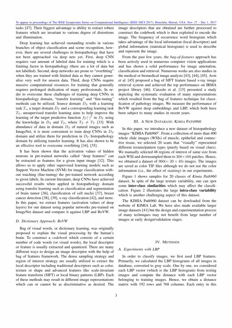
tasks [47]. Their biggest advantage is ability to extract robustfeatures which are invariant to various degree of distortionsand illumination.

Deep learning has achieved oustanding results in variousbranches of object classification and scene recognition, how-ever, there are several challenges in histopathology that havenot been approached via deep nets yet. First, deep CNNrequires vast amount of labeled data for training which is alimiting factor in histopathology (there are a lot of data butnot labelled). Second, deep networks are prone to “overfitting”when they are trained with limited data as they cannot gener-alize very well for unseen data. Third, deep CNNs requiremassive computational resources for training that generallyrequires prolonged dedication of many professionals. In or-der to overcome these challenges of training deep CNNs inhistopathology domain, “transfer learning” and “fine-tuning”methods can be utilized. Source domain DS with a learningtask Ts, a target domain DT and a corresponding learning taskTT , unsupervised transfer learning aims to help improve thelearning of the target predictive function fT (·)7 in DT usingthe knowledge in DS and TS , where TS 6= TT [33]. Withabundance of data in domain DS of natural images such asImageNet, it is more convenient to train deep CNNs in DS

domain and utilize them for prediction in DT histopathologydomain by utilizing transfer learning. It has also shown to bean effective tool to overcome overfitting [34], [35].

It has been shown that the activation values of hiddenneurons in pre-trained networks called “deep features” canbe extracted as features for a given input image [32]. Thisallows us to apply other supervised learning models such asSupport Vector Machine (SVM) for image classification with-out touching (fine-tuning) the pre-trained network accordingto given labels. In current literature, deep CNNs have achievedsuccessful results when applied in histopathology domainusing transfer learning such as classification and segmentationof brain tumor [36], classification of cell nuclei [37], breastcancer detection [38], [39], x-ray classification [42], and more.In this paper, we extract features (activation values of deeplayers) for our dataset using popular networks pre-trained onImageNet dataset and compare it against LBP and BoVW.

D. Dictionary Approach: BoVW

Bag of visual words, or dictionary learning, was originallyproposed to explain the visual processing by the human’sbrain. To construct a codebook which consists of a certainnumber of code words (or visual words), the local descriptoror feature is usually extracted and quantized. There are manydifferent ways to design an image descriptor with the help ofbag of features framework. The dense sampling strategy andregion of interest strategy are usually utilized to extract thelocal descriptor including traditional descriptors such as color,texture or shape and advanced features like scale-invariantfeature transform (SIFT) or local binary patterns (LBP). Eachof these methods may result in different image representationswhich can or cannot be as discriminative as desired. The

image descriptors that are obtained are further processed toconstruct the codebook which is then exploited to encode theimage. The frequency of occurrence word histogram whichtakes advantage of the local information (local descriptor) andglobal information (statistical histogram) is used to describeand represent the image.

From the past few years, the bag-of-features approach hasbeen actively used in numerous computer vision applicationsand has shown a solid performance for image annotation,classification and retrieval. Numerous works are also studies inthe medical or biomedical image analysis [43], [44], [45]. Avniet al. [45] proposed a bag of SIFT feature based x-ray imageretrieval system and achieved the top performance on IRMAproject library [46]. Caicedo et al. [15] presented a studydepicting the systematic evaluation of many representationswhich resulted from the bag of features technique for classi-fication of pathology images. We measure the performance ofBoVW against deep embeddings and LBP, which both havebeen subject to many studies in recent years.

III. A NEW DATABASE: KIMIA PATH960

In this paper, we introduce a new dataset of histopathologyimages “KIMIA Path960”. From a collection of more than 400whole slide images (WSIs) of muscle, epithelial and connec-tive tissue, we selected 20 scans that “visually” representeddifferent texture/pattern types (purely based on visual clues).We manually selected 48 regions of interest of same size fromeach WSI and downsampled them to 308×168 patches. Hence,we obtained a dataset of 960(= 20× 48) images. The imagesare saved as color TIF files although we do not use the colorinformation (i.e., the effect of staining) in our experiments.

Figure 1 shows samples for 20 classes of Kimia Path960dataset. In spite of the large texture variability, one can spotsome inter-class similarities which may affect the classifi-cation. Figure 2 illustrates the large intra-class variabilitywhich is another challenging aspect of this dataset.

The KIMIA Path960 dataset can be dowloaded from thewebsite of KIMIA Lab. We have also made available largerimage datasets [41] but the design and experimentation processof many techniques may not benefit from large number ofimages at early design/validation stages.

IV. METHODS

A. Experiments with LBP

In order to classify images, we first used LBP features.Primarily, we calculated the LBP histograms of all images indatabase, converted to gray scale. One by one, we consideredeach LBP vector (which is the LBP histogram) from testingimages and compute the distance with each LBP vectorbelonging to training images. Hence, we obtain a distancematrix with 192 rows and 768 columns. Each entry in this

3


Fig. 1. Sample images for 20 classes from the Path960 dataset: in spite of the large texture variability, there are some inter-class similarities.

Fig. 2. The Path960 dataset exhibits large intra-class variability: Each row showing four instances of the same class.

matrix corresponds to the distance between images indexedby its row and column. Among these distances, we extract

the ones which have the closest match (smallest distance)to an image in training data. We have considered two types

4


of distance measures, (i) χ2 (Chi-squared) distance, and (ii)Euclidean distance (L2 norm).

B. Experiments with Deep Features

We used two pre-trained deep networks, namely AlexNetmodel [30], [31] and VGG16 model [40]. These networks havebeen trained on a subset of the ImageNet database [28], whichis used in ImageNet Large-Scale Visual Recognition Challenge(ILSVRC) [29]. The model is trained on more than a millionimages and can classify images into 1000 object categories(e.g., mouse, pencil, keyboard, and many animals). As a result,the model has learned local feature representations for a widerange of image categories. This is a common strategy in thecomputer vision to capture this pre-learned models informationas an image feature. Since these two networks have beencreated by different number of layers, we can explore theeffect of deepness in our work as well. The VGG16 consistsof 16 layers with learnable weights: 13 convolutional layers,and 3 fully connected layers, while in the AlexNet there are8 layers with learnable weights: 5 convolutional layers, and 3fully connected layers.

C. Experiments with BoVW

The training images are resized to a fixed dimension(256×256 or 512×512) and the resized image are dividedinto small grids (8×8, 16×16, and also 16×8 with 50%overlap) which will be exploited to extract local descriptors.The uniform LBP with 8 neighbors and radius 1, which hasbeen proved to be a compact and powerful feature is usedas the local descriptor. The size of codebook is set as 800and 1200, respectively, and the initial codewords of codebookare randomly selected from the blocks whose gradient valueare larger than average gradient value. The popular k-meansclustering method is applied to construct the codebook. TheSVM with histogram intersection kernel (IKSVM) is appliedfor the final image classification, and the parameter of SVMis obtained with 3-fold cross validation. The conventionaldistance measurements such as Chi-squared distance (χ2), cityblock distance (L1 norm) and Euclidean distance (L2 norm)are also used for comparison.

V. SIMILARITY VIA DISTANCE CALCULATION

We need to use distance norms like L1 and L2 for(dis)similarity measurement when two feature vectors arebeing compared. For deep features the cosine similarity maybe more appropriate as deep networks generally generate high-dimensional embedding of input images. For LBP, however,the literature generally suggests to use χ2 distance. If p and qrepresent the probability distributions of two events A and Bwith random variables, i = 1, 2, ..., n, the χ2 distance betweenthese two histograms is given by [26], [27]

χ2A,B =

1

2

n∑i=1

([p(i)− q(i)]2

p(i) + q(i)

). (1)

VI. EXPERIMENTS AND RESULTS

In the following sections, we describe the results for threeselected approaches. We used leave-one-out to validate theperformance of LBP and deep features. For BoVW thisvalidation scheme may not be necessarily desirable. Since itis impractical to construct 960 codebooks and also to makesure that the testing images are not used for constructingcodebook, 2 images from each class were randomly selectedand considered to be the testing dataset (40 images in total). Toapproximate the result of leave-one-out strategy, the averageaccuracy of 20 folds is exploited.

A. LBP Results

We generated LBP histograms for all 960 images. For eachof the images, we obtained the best match in the training dataof remaining 959 images. Each query image and its closestmatch should belong to the same category, i.e., among the20 categories {A,B, . . . , T}. We measure the accuracy as thetotal number of cases in which the query image Iq and itsclosest match (in training data) belong to the same categorydivided by 960 when we count the number of elements of theset of correctly classified images Γ:

accuracy =|Γ|960

. (2)

The performance of LBP depends on the radius of neigh-borhood (r) and the number of neighbors considered (p). Aswell, we receive different results for L1, L2 and χ2. Table 1shows the accuracies obtained using the closest match with χ2

distance, and its variations with the two parameters p and r.Similarly, Tables 2 and 3 show the retrieval accuracies usingthe closest match with the Euclidean distance (L2 norm) andthe Manhattan distance (L1 norm), for different p and r values.

The best result for LBP was hence 90.62% and was achievedvia L2 distance. Although the difference to the result of the χ2

is not much (< 1%), but this is an interesting observation sinceχ2 is generally regarded as the distance measure of choicewhen dealing with LBP histograms.

Table 1. LBP classification accuracies (in %) using χ2 distance.

Number of neighbours pr 4 8 12 16 20 241 70.10 84.06 86.46 87.29 88.23 88.232 68.13 82.92 85.83 85.83 85.94 88.023 64.90 81.15 84.17 86.04 86.88 85.624 60.00 78.96 85.94 86.77 88.12 89.065 52.92 74.90 81.04 83.13 84.69 85.83

Table 2. LBP classification accuracies (in %) using L2 norm.


5

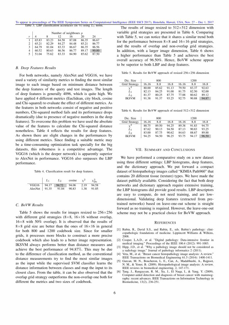
To appear in proceedings of The IEEE Symposium Series on Computational Intelligence (IEEE SSCI 2017), Honolulu, Hawaii, USA, Nov. 27 – Dec 1, 2017Table 3. LBP classification accuracies (in %) using L1 norm.


B. Deep Features Results

For both networks, namely AlexNet and VGG16, we haveused a variety of similarity metrics to finding the most similarimage to each image based on minimum distance betweenthe deep features of the query and test images. The lengthof deep features is generally 4096, which is quite high. Wehave applied 4 different metrics (Euclidean, city block, cosineand Chi-squared) to evaluate the effect of different metrics. Asthe features in both networks consist of negative and positivenumbers, Chi-squared method fails and its performance dropsdramatically (due to presence of negative numbers in the deepfeatures). To overcome this problem we have used the absolutevalue of the features to calculate the Chi-squared distancenonetheless. Table 4 reflects the results for deep features.As shown there are slight changes in the performances byusing different metrics. Since finding a suitable metric maybe a time-consuming optimization task specially for the bigdatasets, this robustness is a competitive advantage. TheVGG16 (which is the deeper network) is apparently superiorto AlexNet in performance. VGG16 also surpasses the LBPperformance.

Table 4. Classification result for deep features.

L1 L2 cosine χ2 χ2abs

VGG16 94.17 94.72 94.06 2.19 94.58AlexNet 91.35 91.04 90.83 1.38 91.05

C. BoVW Results

Table 5 shows the results for images resized to 256×256with different grid strategies (8×8, 16×16 without overlap,16×8 with 50% overlap). It is observed that the results of8×8 grid size are better than the ones of 16×16 in generalfor both 800 and 1200 codebook size. Since for smallergrids, it processes more blocks to construct a more precisecodebook which also leads to a better image representation.IKSVM always performs better than distance measures andachieve the best performance of 94.87%. This may be dueto the difference of classification method, as the conventionaldistance measurements try to find the most similar imagesas the input while the supervised SVM classifier learns thedistance information between classes and map the input to itsclosest class. From the table, it can be also observed that theoverlap grid strategy outperforms the non-overlap one both fordifferent the metrics and two sizes of codebook.

The results of image resized to 512×512 dimension withvariable grid strategies are presented in Table 6. Comparingwith Table 5, we can notice that it shares a similar trend bothfor the performance between 8×8 and 16×16 grid strategies,and the results of overlap and non-overlap grid strategies.In addition, with a larger image dimension, Table 6 showsa higher performance than Table 5 and achieves the bestoverall accuracy of 96.50%. Hence, BoVW scheme appearto be superior to both LBP and deep features.

Table 5. Results for BoVW approach of resized 256×256 dimension

Dic. Size 800 1200Grid Strategy 16 16 8 8 16 8 16 16 8 8 16 8

χ2 80.00 85.62 91.13 79.50 83.37 92.63L1 82.13 84.25 91.00 81.75 82.50 92.00L2 81.37 80.25 87.75 77.88 80.62 89.12

IKSVM 91.38 91.37 93.25 92.75 90.88 94.87

Table 6. Results for BoVW approach of resized 512×512 dimension

Dic. Size 800 1200Grid Strategy 16 16 8 8 16 8 16 16 8 8 16 8

χ2 88.75 89.50 94.25 89.38 91.83 94.75L1 87.62 90.13 94.50 87.13 90.83 93.25L2 83.00 87.75 90.62 84.63 88.67 89.88

IKSVM 94.25 94.50 96.25 93.75 94.17 96.50

VII. SUMMARY AND CONCLUSIONS

We have performed a comparative study on a new datasetusing three different settings: LBP histograms, deep features,and the dictionary approach. We put forward a compactdataset of histopathology images called “KIMIA Path960” thatcontains 20 different tissue (texture) types. We have made thedataset publicly available. Considering the fact that both deepnetworks and dictionary approach require extensive training,the LBP histograms did provide good results. LBP descriptorsare easy to compute, do not need training, and are low-dimensional. Validating deep features (extracted from pre-trained networks) based on leave-one-out scheme is straightforward as no training is required. However, the leave-one-outscheme may not be a practical choice for BoVW approach.

REFERENCES

[1] Rubin, R., David S.S., and Rubin, E., eds. Rubin’s pathology: clini-copathologic foundations of medicine. Lippincott Williams & Wilkins,2008.

[2] Cooper, L.A.D., et al. ”Digital pathology: Data-intensive frontier inmedical imaging.” Proceedings of the IEEE 100.4 (2012): 991-1003.

[3] Hipp, J.D., et al. ”Why a pathology image should not be considered asa radiology image.” Journal of pathology informatics 2 (2011).

[4] Veta, M., et al. ”Breast cancer histopathology image analysis: A review.”IEEE Transactions on Biomedical Engineering 61.5 (2014): 1400-1411.

[5] Gurcan, M. N., Boucheron, L. E., Can, A., Madabhushi, A., Rajpoot,N. M., & Yener, B. (2009). Histopathological image analysis: A review.IEEE reviews in biomedical engineering, 2, 147-171.

[6] Tang, J., Rangayyan, R. M., Xu, J., El Naqa, I., & Yang, Y. (2009).Computer-aided detection and diagnosis of breast cancer with mammog-raphy: recent advances. IEEE Transactions on Information Technology inBiomedicine, 13(2), 236-251.

6


[7] Rubin, R., Strayer, D. S., & Rubin, E. (Eds.). (2008). Rubin’s pathol-ogy: clinicopathologic foundations of medicine. Lippincott Williams &Wilkins.

[8] Weind, K. L., Maier, C. F., Rutt, B. K., & Moussa, M. (1998). Invasivecarcinomas and fibroadenomas of the breast: comparison of microvesseldistributions–implications for imaging modalities. Radiology, 208(2), pp.477-483.

[9] Bartels, P. H., Thompson, D., Bibbo, M., & Weber, J. E. (1992). Bayesianbelief networks in quantitative histopathology. Analytical and quantitativecytology and histology/the International Academy of Cytology [and]American Society of Cytology, 14(6), pp.459-473.

[10] Datar, M., Padfield, D., & Cline, H. (2008, May). Color and texturebased segmentation of molecular pathology images using HSOMs. InBiomedical Imaging: From Nano to Macro. ISBI 2008. 5th IEEE Inter-national Symposium on, pp. 292-295.

[11] Caicedo, J. C., Gonzalez, F. A., & Romero, E. (2008, January). Asemantic content-based retrieval method for histopathology images. InAsia Information Retrieval Symposium, Springer Berlin Heidelberg, pp.51-60.

[12] Zheng, L., Wetzel, A. W., Gilbertson, J., & Becich, M. J. (2003). Designand analysis of a content-based pathology image retrieval system. IEEETransactions on Information Technology in Biomedicine, 7(4), pp. 249-255.

[13] Lam, R. W., Ip, H. H. S., Cheung, K. K., Tang, L. H., & Hanka, R.(2000). A multi-window approach to classify histological features. InPattern Recognition, 2000. Proceedings. 15th International Conferenceon, Vol. 2, pp. 259-262.

[14] Tang, H. L., Hanka, R., & Ip, H. H. S. (2003). Histological imageretrieval based on semantic content analysis. IEEE Transactions onInformation Technology in Biomedicine, 7(1), pp. 26-36.

[15] Caicedo, J. C., Cruz, A., & Gonzalez, F. A. (2009, July). Histopathologyimage classification using bag of features and kernel functions. InConference on Artificial Intelligence in Medicine in Europe . SpringerBerlin Heidelberg, pp. 126-135.

[16] Jadhav, A. S., Banerjee, S., Dutta, P. K., Paul, R. R., Pal, M., Banerjee, P.,... & Chatterjee, J. (2006, June). Quantitative analysis of histopathologicalfeatures of precancerous lesion and condition using image processingtechnique. In Computer-Based Medical Systems, 2006. CBMS 2006. 19thIEEE International Symposium on, pp. 231-236.

[17] Pal, M., Chaudhuri, S. R., Jadav, A., Banerjee, S., Paul, R. R., Dutta, P.K., ... & Chaudhuri, K. (2008). Quantitative dimensions of histopatholog-ical attributes and status of GSTM1?GSTT1 in oral submucous fibrosis.Tissue and Cell, 40(6), pp. 425-435.

[18] Ferrari, R. J., Rangayyan, R. M., Desautels, J. L., & Frare, A. F. (2001).Analysis of asymmetry in mammograms via directional filtering withGabor wavelets. IEEE Transactions on Medical Imaging, 20(9), pp. 953-964.

[19] Marghani, K. A., Dlay, S. S., Sharif, B. S., & Sims, A. J. (2003, May).Morphological and texture features for cancer tissues microscopic images.In Medical Imaging 2003. International Society for Optics and Photonics,pp. 1757-1764.

[20] Kong, J., Sertel, O., Shimada, H., Boyer, K. L., Saltz, J. H., & Gurcan,M. N. (2009). Computer-aided evaluation of neuroblastoma on whole-slide histology images: Classifying grade of neuroblastic differentiation.Pattern Recognition, 42(6), pp. 1080-1092.

[21] Unay, D., & Ekin, A. (2008, May). Intensity versus texture for medicalimage search and retrival. In Biomedical Imaging: From Nano to Macro,ISBI 2008. 5th IEEE International Symposium on, pp. 241-244.

[22] Oliver, A., Llado, X., Freixenet, J., & Marta, J. (2007). False positivereduction in mammographic mass detection using local binary patterns.Medical Image Computing and Computer-Assisted Intervention? MIC-CAI 2007, pp. 286-293.

[23] Ojala, T., Pietikainen, M., & Harwood, D. (1994, October). Performanceevaluation of texture measures with classification based on Kullbackdiscrimination of distributions. In Pattern Recognition, 1994. Vol. 1-Conference A: Computer Vision & Image Processing., Proceedings ofthe 12th IAPR International Conference on, Vol. 1, pp. 582-585.

[24] Wang, X., Han, T. X., & Yan, S. (2009, September). An HOG-LBPhuman detector with partial occlusion handling. In Computer Vision, 2009IEEE 12th International Conference on, pp. 32-39.

[25] Adamo, F., Carcagni, P., Mazzeo, P. L., Distante, C., & Spagnolo, P.(2014, August). TLD and Struck: A Feature Descriptors ComparativeStudy. In International Workshop on Activity Monitoring by MultipleDistributed Sensing. Springer International Publishing, pp. 52-63.

[26] Asha, V., Bhajantri, N. U., & Nagabhushan, P. (2011). GLCM?basedchi?square histogram distance for automatic detection of defects onpatterned textures. International Journal of Computational Vision andRobotics, 2(4), pp. 302–313.

[27] Pele, O., & Werman, M. (2010, September). The quadratic-chi histogramdistance family. In European conference on computer vision . SpringerBerlin Heidelberg, pp. 749–762.

[28] ImageNet. http://www.image-net.org[29] Russakovsky, O., Deng, J., Su, H., et al. ImageNet Large Scale Visual

Recognition Challenge. International Journal of Computer Vision (IJCV).Vol 115, Issue 3, 2015, pp. 211–252

[30] Krizhevsky, Alex, Ilya Sutskever, and Geoffrey E. Hinton. ImageNetClassification with Deep Convolutional Neural Networks. Advances inneural information processing systems. 2012.

[31] BVLC AlexNet Model. https://github.com/BVLC/caffe/tree/master/models/bvlc_alexnet.

[32] Hou, L., K. Singh, D. Samaras, T. M. Kurc, Y. Gao, R. J. Seid-man, and J. H. Saltz. Automatic Histopathology Image Analysis withCNNs. In 2016 New York Scientific Data Summit (NYSDS), 16, 2016.doi:10.1109/NYSDS.2016.7747812.

[33] Pan, S.J., Yang, Q., 2010. A Survey on Transfer Learning. IEEETransactions on Knowledge and Data Engineering 22, pp. 1345–1359.doi:10.1109/TKDE.2009.191

[34] Oquab, M., Bottou, L., Laptev, I., Sivic, J.: Learning and transferringmid-level image representations using convolutional neural networks. In:CVPR, IEEE. pp. 1717–1724 (2014).

[35] Yosinski, J., Clune, J., Bengio, Y., Lipson, H.: How transferable arefeatures in deep neural networks? In: Advances in Neural InformationProcessing Systems. pp. 3320–3328 (2014).

[36] Xu, Y., Jia, Z., Ai, Y., Zhang, F., Lai, M., Eric, I. and Chang, C.,2015, April. Deep convolutional activation features for large scale braintumor histopathology image classification and segmentation. In Acous-tics, Speech and Signal Processing (ICASSP), 2015 IEEE InternationalConference on, pp. 947-951.

[37] Bayramoglu, N. and Heikkila J., 2016, October. Transfer Learning forCell Nuclei Classification in Histopathology Images. In ECCV Workshops(3), pp. 532-539.

[38] Wang, D., Khosla, A., Gargeya, R., Irshad, H. and Beck, A.H., 2016.Deep learning for identifying metastatic breast cancer. arXiv preprintarXiv:1606.05718.

[39] Cruz-Roa, A., Basavanhally, A., Gonzalez , F., Gilmore, H., Feldman,M., Ganesan, S., Shih, N., Tomaszewski, J. and Madabhushi, A., 2014,March. Automatic detection of invasive ductal carcinoma in whole slideimages with convolutional neural networks. In SPIE medical imaging,Vol. 9041, pp. 904103–904103.

[40] Simonyan K, Zisserman A. Very deep convolutional networks for large-scale image recognition. arXiv preprint arXiv:1409.1556. 2014 Sep 4.

[41] Morteza Babaie, Shivam Kalra, Aditya Sriram, Christopher Mitcheltree,Shujin Zhu, Amin Khatami, Shahryar Rahnamayan, Hamid R Tizhoosh,Classification and Retrieval of Digital Pathology Scans: A New Dataset.CVMI Workshop @ CVPR 2017.

[42] Khatami A, Babaie M, Khosravi A, Tizhoosh HR, Salaken SM, Naha-vandi S. A deep-structural medical image classification for a Radon-basedimage retrieval. InElectrical and Computer Engineering (CCECE), 2017IEEE 30th Canadian Conference on 2017 Apr 30, pp. 1-4.

[43] Wang J, Liu P, She MF, Nahavandi S, Kouzani A. Bag-of-wordsrepresentation for biomedical time series classification. Biomedical SignalProcessing and Control. 2013 Nov 30;8(6), pp. 634-44.

[44] Bouslimi R, Messaoudi A, Akaichi J. Using a bag of words forautomatic medical image annotation with a latent semantic. arXiv preprintarXiv:1306.0178. 2013 Jun 2.

[45] Avni U, Greenspan H, Konen E, Sharon M, Goldberger J. X-raycategorization and retrieval on the organ and pathology level, usingpatch-based visual words. IEEE Transactions on Medical Imaging. 2011Mar;30(3), pp. 733-46.

[46] Lehmann TM, Gold MO, Thies C, Fischer B, Spitzer K, KeysersD, Ney H, Kohnen M, Schubert H, Wein BB. Content-based imageretrieval in medical applications. Methods of information in medicine.2004 Oct;43(4), pp. 354-61.

[47] Zejmo, Micha, Marek Kowal, Jozef Korbicz, and Roman Monczak.“Classification of Breast Cancer Cytological Specimen Using Convolu-tional Neural Network.” Journal of Physics: Conference Series 783, no.

1 (2017): 012060. doi:10.1088/1742-6596/783/1/012060.

7

https://github.com/BVLC/caffe/tree/master/models/bvlc_alexnet

https://github.com/BVLC/caffe/tree/master/models/bvlc_alexnet

Documents

A Comparative Study of CNN, BoVW and LBP for Classiﬁcation ... · characteristics. This paper is a comparative study describing the potential of using local binary patterns (LBP),