University of Central Florida University of Central Florida

STARS STARS

Electronic Theses and Dissertations, 2004-2019

2006

A Comparative Study Of Ant Colony Optimization A Comparative Study Of Ant Colony Optimization

Matthew Becker University of Central Florida

Part of the Mathematics Commons

Find similar works at: https://stars.library.ucf.edu/etd

University of Central Florida Libraries http://library.ucf.edu

This Masters Thesis (Open Access) is brought to you for free and open access by STARS. It has been accepted for

inclusion in Electronic Theses and Dissertations, 2004-2019 by an authorized administrator of STARS. For more

information, please contact STARS@ucf.edu.

STARS Citation STARS Citation Becker, Matthew, "A Comparative Study Of Ant Colony Optimization" (2006). Electronic Theses and Dissertations, 2004-2019. 6148. https://stars.library.ucf.edu/etd/6148

A COMPARATIVE STUDY OF ANT COLONY OPTIMIZATION

by

MATTHEW BECKER B.S., Kansas State University, 1987

A thesis submitted in partial fulfillment of the requirements for the degree of Master of Science

in the Department of Mathematical Science in the College of Sciences

at the University of Central Florida Orlando, Florida

Summer Term 2006

© 2006 Matthew Becker

ii

ABSTRACT

Ant Colony Optimization (ACO) belongs to a class of biologically-motivated approaches

to computing that includes such metaheuristics as artificial neural networks, evolutionary

algorithms, and artificial immune systems, among others. Emulating to varying degrees the

particular biological phenomena from which their inspiration is drawn, these alternative

computational systems have succeeded in finding solutions to complex problems that had

heretofore eluded more traditional techniques. Often, the resulting algorithm bears little

resemblance to its biological progenitor, evolving instead into a mathematical abstraction of a

singularly useful quality of the phenomenon. In such cases, these abstract computational models

may be termed biological metaphors. Mindful that a fine line separates metaphor from

distortion, this paper outlines an attempt to better understand the potential consequences an

insufficient understanding of the underlying biological phenomenon may have on its

transformation into mathematical metaphor. To that end, the author independently develops a

rudimentary ACO, remaining as faithful as possible to the behavioral qualities of an ant colony.

Subsequently, the performance of this new ACO is compared with that of a more established

ACO in three categories: (1) the hybridization of evolutionary computing and ACO, (2) the

efficacy of daemon actions, and (3) theoretical properties and convergence proofs.

iii

TABLE OF CONTENTS

LIST OF FIGURES ....................................................................................................................... vi

LIST OF ACRONYMS ................................................................................................................ vii

CHAPTER ONE: INTRODUCTION............................................................................................. 1

CHAPTER TWO: LITERATURE REVIEW................................................................................. 3

The Ant Colony Optimization Metaheuristic ......................................................................... 3

Problem Characterization.................................................................................................... 4

Behavior of Virtual Ants..................................................................................................... 6

The Metaheuristic ............................................................................................................... 8

CHAPTER THREE: A CONCISE HISTORY OF ACO ............................................................. 11

ACO as Biologically-Inspired Computing............................................................................ 11

Historical Development ........................................................................................................ 14

Ant System and the Traveling Salesman Problem................................................................ 15

Ant System and its Successors.............................................................................................. 17

CHAPTER FOUR: THEORETICAL CONSIDERATIONS ...................................................... 20

Convergence Proofs .............................................................................................................. 21

Convergence in Value....................................................................................................... 23

Convergence in Solution................................................................................................... 26

Further Considerations...................................................................................................... 31

Summary ........................................................................................................................... 32

CHAPTER FIVE: EVOLUTIONARY COMPUTING/ACO HYBRIDS.................................... 35

iv

A Primer on Evolutionary Programming and Genetic Algorithms ...................................... 35

Evolution and the Ant ........................................................................................................... 37

Results................................................................................................................................... 38

CHAPTER SIX: CONCLUSIONS............................................................................................... 40

LIST OF REFERENCES.............................................................................................................. 41

v

LIST OF FIGURES

Figure 1. The ACO metaheuristic in pseudo-code. The procedure DaemonActions() is optional

and refers to centralized actions executed by a daemon possessing global knowledge. ........ 9

Figure 2. High-level pseudo-code for the procedure PheromoneUpdate. ................................... 23

Figure 3. Steiner tree solution generated by Matlab ACO with colony-level selection. .............. 39

vi

LIST OF ACRONYMS

ACO Ant Colony Optimization

ACS Ant Colony System

AS Ant System

EP Evolutionary Programming

GA Genetic Algorithms

MMAS Max-Min Ant System

TSP Traveling Salesman Problem

vii

CHAPTER ONE: INTRODUCTION

This paper explores the effect that the hybridization of evolutionary computing and Ant

Colony Optimization (ACO) methods, the inclusion of various daemon actions, and the

exclusion of such phenomena as phase transitions in ant colony foraging behavior may have on

the efficacy of the family of algorithms comprising the Ant Colony Optimization metaheuristic.

The quality of Ant System (AS), the original ACO algorithm, that most distinguished it from

such related metaheuristics as evolutionary computing, genetic algorithms, etc., was its faithful

emulation of the highly coordinated behavior of actual ants during foraging, in particular. The

eusocial insect phenomenon of order absent hierarchical control was the fundamental inspiration

that set the ACO ball in motion [7]. And yet, paradoxically, the development of this particular

category of computational methods has been marked by an inexorable abandonment of its

founding precepts [10]. In fact, the first significant improvement made to AS was the

incorporation of the so-called elitist strategy, the first of the daemon actions to be introduced into

the algorithm.

While it is incontrovertible that the addition of various global controls, elitist strategy

among them, has improved the performance of successive ACO incarnations, it is the author’s

suspicion that these enhancements are, nevertheless, in some measure at odds with the eminently

distributed nature of an ant colony and their inclusion may come at a cost: namely, the resultant

loss of autonomy among the ants and the inevitable diminution of their collective contribution to

the algorithm’s various applications.

This report is divided into five primary sections. Immediately following the introduction

is a chapter in which the current literature on selected optimization techniques and ACO in

1

particular is review. The third section provides a concise history of the ACO metaheuristic.

Section four focuses on the underlying principles and methodology of ACO. The fifth major

section provides a conclusion. It also considers additional research and discusses the possibilities

for future work based on this research.

2

CHAPTER TWO: LITERATURE REVIEW

The Ant Colony Optimization Metaheuristic

Artificial ants used in ACO are stochastic solution construction procedures that

probabilistically build a solution by iteratively adding solution components to partial solutions

while taking into account (i) heuristic information on the problem being solved, if available, and

(ii) artificial pheromone trails that change dynamically at run-time to reflect the ants’ acquired

search experience.

The interpretation of ACO as an extension of construction heuristics is appealing for

several reasons. First, a stochastic component in ACO allows the ants to build a wide variety of

solutions and consequently to explore a much larger number of solutions than do conventional

greedy heuristics. Second, the concurrent use of heuristic information, which is readily available

for many problems, can direct the ants more quickly towards the most promising solutions.

Third, the record of an ant’s exploration of the solution space can be used to influence solution

construction in future iterations of the algorithm in a manner reminiscent of reinforcement

learning [18]. Fourth, given that a colony may comprise a multitude of individual ants, with

built-in redundancy as far as the eye can see, the algorithm is profoundly robust and in many

ACO applications, the collective interaction of a population of agents is required to efficiently

solve a problem.

The range of applications which may be solved by ACO algorithms is vast. In principle,

ACO can be applied to any discrete optimization problem for which some solution construction

mechanism can be conceived. In the following section, a generic problem for which ACO might

3

be tasked to construct solutions is described, and the ants’ behavior during a typical solution

search is explored.

Problem Characterization

Consider a minimization problem (S, f, Ω), in which S is the set of candidate solutions, f

is the objective function which assigns to each candidate solution s an objective function , or cost

f(s,t), and Ω is a set of constraints. The goal is to find a globally optimal solution sopt S (i.e., a

minimum cost solution that satisfies the constraints Ω).

A combinatorial optimization problem (S, f, Ω) such as this can be characterized as

follows:

• A finite set C = c1, c2,…..,cNc of components.

• The states of the problem are defined in terms of all possible sequences

x = <ci, cj,…,ch,…> over the elements of C. The length of a sequence x is the number of

components in the sequence and is expressed as |x|.

• The finite set of constraints Ω defines the set of feasible states Χ , with . Χ ⊆ Χ

• A set S* of feasible solutions is given, with and *S ⊆ Χ * .S S⊆

• A cost f(s,t) is associated with each candidate solution s S.

• In some cases a cost, or the estimate of a cost, J(xi,t), can be associated with states other

than solutions. If xj can be obtained by adding solution components to a state xi then J(xi

,t) J(xj,t). Note that J(s,t) f(s,t).

Given this translation of the problem into terminology understood by the algorithm’s

artificial ants, they set about building solutions by moving on the construction graph G = (C, L),

4

where the vertices are the components C and the set L fully connects the components C

(elements of L are called connections). The problem constraints Ω are implemented in directions

given to the artificial ants, as will be explained in the next section. The choice of implementing

the constraints in the construction policy of the artificial ants affords the algorithm a measure of

flexibility. In fact, depending on the combinatorial optimization problem being considered, it

may be more reasonable to implement more stringent constraints, allowing ants to build only

feasible solutions. Conversely, the problem may be one that is better served by ants permitted to

construct impracticable solutions (i.e., candidate solutions in S\S*) that will be penalized to a

degree commensurate with their distance from viable solutions

5

Behavior of Virtual Ants

Virtual ants may be thought of as stochastic construction procedures which build solu-

tions while moving on the construction graph G = (C, L). Ants do not move arbitrarily on G, but

rather follow a construction policy that is a function of the problem constraints Ω. Components

ci C and connections lij L may possess a corresponding pheromone trail τ, designated τi if

associated with components and τij if associated with connections. A heuristic value η (ηi and ηij,

as above) represents a priori information about either specific qualities of a problem or run-time

information. In many cases, η is the cost, or an estimate of the cost, of extending the current

state. These values define the initial parameters that govern the ants’ stochastic motion on the

graph.

More precisely, each ant k of the colony has the following properties:

• It searches the graph G = (C, L) for feasible solutions s of minimal cost (i.e., solutions

such that sˆ =min (s,t).sf f

• It has memory Mk that it uses to store information regarding the path that it has

negotiated. Memory can be used (i) to build feasible solutions (i.e., to implement

constraints Ω), (ii) to evaluate a discovered solution, and (iii) to retrace the path

backwards in order to deposit pheromone.

• It can be assigned an initial state xk and one or more termination conditions e

k. Usually,

the initial state is expressed either as a unit length sequence (i.e., a single component

sequence) or an empty sequence.

6

• When in state xr = < xr-1, i> and if no termination condition has been satisfied, an ant

moves to a node j in its neighborhood and advances to a state kiN

< xr, j> X. Typically, motion in the direction of feasible states is favored, and may

be attained through properly defined heuristic values η or by means of the ant’s own

memory.

• It selects each move according to a probabilistic decision rule. This rule is a function of

(i) local pheromone trails and heuristic values that it has encountered, (ii) the ant’s

memory, and (iii) the relevant problem constraints.

• The construction procedure of ant k ceases when at least one of the termination

conditions ek is satisfied.

• When adding a component cj to the current solution, an ant can update its pheromone trail

or that of the corresponding connection. This action is referred to as online step-by-step

pheromone update.

• Once a solution has been constructed, an ant can retrace its path backwards and update

the pheromone trails of used components or connections. This action is called online

delayed pheromone update.

It is important to note that each ant moves independently and is sufficiently complex to

find its own (probably poor) solution to the problem under consideration. Usually, quality

solutions emerge as a consequence of interaction among the ants, characterized by indirect

communication that is mediated by the information ants read and write to the variables storing

pheromone trail values. (This indirect means of communication via pheromone is called

stigmergy.) One might consider this system a distributed learning process within which the

7

agents, or ants, are not adaptive themselves; rather, individual ants serve to modify the way in

which the problem is represented and perceived by other ants.

The Metaheuristic

Informally, the behavior of ants in an ACO algorithm may be summarized as follows: A

colony of ants concurrently and asynchronously move through adjacent states of a problem by

building paths on the aforementioned solution space G. The ants move by applying a stochastic

local decision-making policy that makes use of pheromone trails and heuristic information. As

they move, ants incrementally build solutions to the optimization problem. Once an ant has built

a solution, or as the solution is constructed, an ant evaluates its contribution to the solution and

deposits pheromone upon trails representing the associated components or connections. This

pheromone information provides guidance to future ants in their search for a solution.

In addition to the activity of ants, an ACO algorithm includes two more procedures:

pheromone trail evaporation and daemon actions (this last component being optional).

Pheromone evaporation is the process by which pheromone intensity decreases over time on

trails traversed (i.e., partial trial solutions) by ants. The relatively ephemeral nature of

pheromone reduces the likelihood of premature convergence by the algorithm towards a sub-

optimal region (or to a local rather than a global minimum, for example)

8

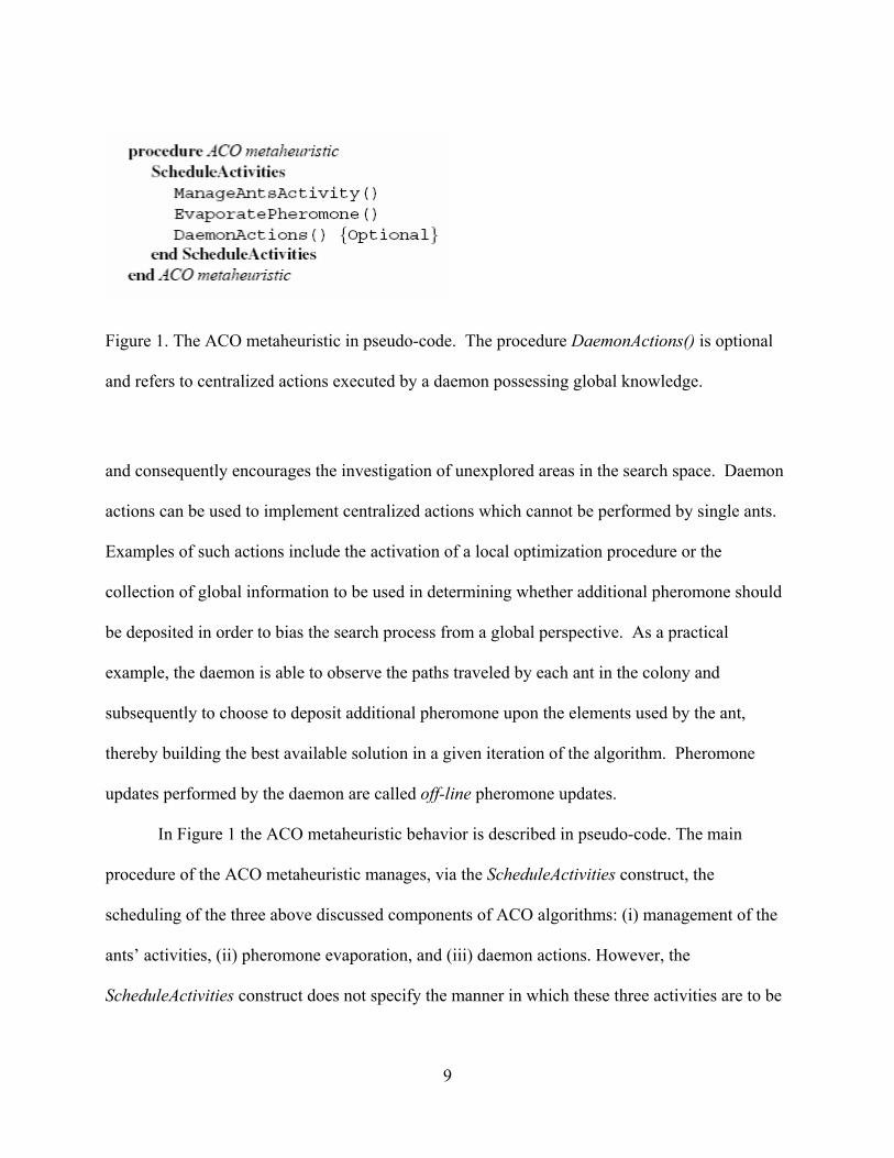
Figure 1. The ACO metaheuristic in pseudo-code. The procedure DaemonActions() is optional

and refers to centralized actions executed by a daemon possessing global knowledge.

and consequently encourages the investigation of unexplored areas in the search space. Daemon

actions can be used to implement centralized actions which cannot be performed by single ants.

Examples of such actions include the activation of a local optimization procedure or the

collection of global information to be used in determining whether additional pheromone should

be deposited in order to bias the search process from a global perspective. As a practical

example, the daemon is able to observe the paths traveled by each ant in the colony and

subsequently to choose to deposit additional pheromone upon the elements used by the ant,

thereby building the best available solution in a given iteration of the algorithm. Pheromone

updates performed by the daemon are called off-line pheromone updates.

In Figure 1 the ACO metaheuristic behavior is described in pseudo-code. The main

procedure of the ACO metaheuristic manages, via the ScheduleActivities construct, the

scheduling of the three above discussed components of ACO algorithms: (i) management of the

ants’ activities, (ii) pheromone evaporation, and (iii) daemon actions. However, the

ScheduleActivities construct does not specify the manner in which these three activities are to be

9

scheduled nor whether there should exist some coordination among them; it is the prerogative of

the programmer to specify the manner in which these three procedures should interact.

10

CHAPTER THREE: A CONCISE HISTORY OF ACO

The first ACO algorithm proposed was Ant System (AS). AS was applied to some rather

trivial examples of the Traveling Salesman Problem (TSP) with circuits of up to 75 cities.

Although it was able to match the performance of other general-purpose heuristics like evo-

lutionary computation [8, 13], for example, AS ultimately proved not to be competitive with

state-of-the-art algorithms that had been specifically designed for the TSP, particularly as the

numbers of cities were increased beyond its proverbial comfort zone. Consequently, a

substantial amount of research was directed towards developing ACO algorithms demonstrating

better performance than AS when applied to the TSP and similar challenging tasks.

Within this chapter, the biological metaphor upon which AS and ACO are based is

introduced and discussed. An abridged history of the various algorithms comprising the

intermediate developmental stages that mark the evolution of the ACO heuristic from the origi-

nal AS incarnation to the most recent ACO algorithms is also included.

ACO as Biologically-Inspired Computing

In many species of ants, individual ants deposit pheromone—a chemical that may be

sensed by other ants—as an indirect means of communication [9]. Through the deposition of

pheromone, they create a trail that is used, for example, to mark a path from the nest to food

sources and back. By sensing pheromone trails, foragers are able to find their way to food that

11

has been discovered by other ants. Moreover, they are capable of exploiting pheromone trails to

choose the shortest among the available paths.

Deneubourg and colleagues [3, 15] used a double bridge connecting a nest of ants and a

food source to study the phenomenon of pheromone trails, observing behavior in controlled

experimental conditions. They ran a number of experiments in which they varied the ratio

between the lengths of the two branches of the bridge. The most relevant of these experiments to

the development of AS was the one in which the branches were of different lengths. In this

experiment, a laboratory colony of Argentine ants (Iridomyrmex humilis) was initially allowed to

move freely between the nest and the food source, and the shifting percentages of ants choosing

one or the other of the two branches were recorded over time. Although in the initial phase,

random oscillations in the relative amounts of ant traffic would occur, an overwhelming majority

of the experiments found all the ants traveling via the shorter of the two branches.

This result can be explained as follows: Because there is no pheromone on the available

paths initially, the ants have no preference and select with equal probability either of the two

branches. Therefore, it can be expected that, on average, half of the ants will select the shorter

branch and half the longer, although stochastic oscillations may occasionally favor one branch

over the other. However, because one branch is shorter (and assuming all ants travel at the same

speed), the ants choosing the shorter route will be the first to reach the food and, consequently,

the first to begin their return trip. As they decide whether to return via the short or the long

branch, the higher level of pheromone on the short branch biases their decision in its favor.

Therefore, pheromone starts to accumulate faster on the short branch, which will eventually be

used exclusively by a large percentage of the ants.

12

That this pheromone-based communication among ants inspired AS and subsequent

algorithms is clear: the double bridge was substituted by a graph and pheromone trails by virtual

pheromone trails. Also, because artificial ants are tasked with solving problems much more

complicated than those solved by real ants, artificial ants are endowed with extra capacities such

as superior memory (used to implement constraints and to allow the ants to retrace their path

back to the nest without error) and the capacity to precisely deposit a quantity of pheromone

proportional to the quality of the solution produced (a similar behavior is observed in some real

ant species in which the quantity of pheromone deposited while returning to the nest from a food

source is proportional to the quality of the food source found [3]).

Subsequent to the advent of AS, new algorithms have been developed that, though they

retain some elements of the original biological inspiration, are less a near-faithful re-creation of

the natural phenomena of ant colony foraging behavior but are instead increasingly motivated by

the need to improve ACO algorithms in order that they might compete with state-of-the-art algo-

rithms. Nevertheless, many aspects of the original Ant System remain:

• a requirement for a colony of ants.

• the role of autocatalysis (any process by which a decision taken at time t increases the

probability of making the same decision at time T > t by means of the implementation of

positive feedback).

• cooperative behavior among ants managed by virtual pheromone trails. the probabilistic

construction of solutions biased by pheromone and local heuristic information.

• pheromone updating apportioned according to solution quality.

• the evaporation of pheromone.

13

All of these elements survive as integral elements in more modern ACO algorithms. Ant

algorithms are receiving increasing attention within the scientific community (consult for

examples: [8, 9, 11]) and are developing a reputation as novel and effective approaches to

solving problems of distributed control and optimization.

Historical Development

As mentioned previously, AS was the first example of an ACO algorithm to be proposed

in the literature. In fact, AS was originally conceived as three versions of the same algorithm:

ant-cycle, ant-density, and ant-quantity. These three algorithms were proposed in Marco

Dorigo’s doctoral dissertation [20] and first appeared in a technical report [5] that was published

a few years later in the IEEE Transactions on Systems, Man, and Cybernetics [3].

While in the ant-density and ant-quantity components of the algorithm, the ants update

the pheromone immediately following an excursion from one city to another, ant-cycle’s

pheromone update was performed only after all ants had constructed their tours, and the amount

of pheromone deposited by each ant was determined as a function of the solution quality.

Because ant-cycle performed more successfully than the other two variants, it later came to be

called simply Ant System, while work on the other two algorithms was abandoned.

The primary merit of AS, the computational capabilities of which showed promise but

were not competitive with more established approaches, was to stimulate a number of

researchers, mostly in Europe, to develop extensions and improvements to its fundamental

design.

14

Ant System and the Traveling Salesman Problem

The Traveling Salesman Problem (TSP) is a so-called NP-hard combinatorial

optimization problem that has attracted a considerable amount of research effort [4, 9, 12]. The

TSP is an important problem also in the context of Ant Colony Optimization in that it is the

problem to which the original AS was initially applied [5, 19], and it is frequently used as a

benchmark to test new ideas and algorithmic variants.

In AS, each ant is initially situated on a randomly chosen city with a memory that will

store the partial solution it devises with each iteration of the algorithm. Subsequently, an ant

moves from city to city. While at city i, for example, an ant k will travel to an as yet unvisited

city j with a probability given by

(1)

where ηij = 1/dij is heuristic information, α and β determine the relative contributions of

pheromone and heuristic information, and is the plausible neighborhood of ant k (i.e., the

collection of cities not yet visited by ant k ). Parameters α and β exert the following influence

on the algorithm’s behavior: If α = 0, the selection probabilities are proportional to [ηij ]β,

making the nearest cities more likely be selected. In this case, AS corresponds to a classical

stochastic greedy algorithm (with multiple starting points since ants are initially randomly

distributed on the cities). If β = 0, pheromone amplification acts alone on the population of

artificial ants, leading to inevitable stagnation and the generation of partial solutions that are

kiN

15

most likely to be significantly suboptimal [16]. (Search stagnation is defined in [2] as a situation

whereby all ants ultimately follow the same path and construct identical solutions.)

Solution construction ends after each ant has completed a tour, that is, after each ant has

constructed a sequence of length n. The pheromone trails are then updated. In AS, this is

achieved by initially reducing the amount of pheromone on all trails by a constant factor (i.e.,

pheromone evaporation) and then allowing each ant to deposit pheromone on the arcs that

describe its own partial solution:

(2)

where 0 < ρ ≤ 1 is the pheromone evaporation rate and m is the number of ants. The parameter ρ

prevents unlimited accumulation of pheromone, thus allowing the algorithm to dispense of poor

solutions. Upon arcs which are not chosen by ants, the associated pheromone strength will

decrease exponentially with the number of iterations. represents the amount of

pheromone ant k deposits on the arcs and is defined as

(t)kijτ∆

(3)otherwise.

if arc (i, j) is used by ant k.

where is the length of the kth ant’s tour. According to equation (3), the shorter an ant’s

tour, the more pheromone is received by its constituent arcs. In general, those arcs traversed by

many ants and contained within shorter tours receive more pheromone and therefore are more

likely to be chosen as potentially viable solutions in subsequent iterations of the algorithm.

kL ( )t

16

Ant System and its Successors

Because AS was largely uncompetitive with state-of-the-art algorithms for TSP,

researchers began to extend the algorithm in order to improve its performance. An initial

improvement, deemed the elitist strategy, was introduced in [13, 22]. An algorithm employing

elitist strategy awards the best tour since the algorithm’s launch (called Tgb , where gb stands for

global-best) a considerable additional weight. In practice, every time the pheromone trails are

refreshed, those belonging to the edges of the global-best tour receive an additional amount of

pheromone. For these edges, equation (3) becomes:

(3a)

The arcs of Tgb are therefore reinforced with a quantity of e • 1/Lgb , where Lgb is the

length of Tgb and e is a positive integer. Note that this version of pheromone replenishment is the

first instance of daemon action to be implemented in the ACO family of algorithms.

Other improvements, described below, include the so-called rank-based version of Ant

System (ASrank ), MAX -MIN Ant System (MMAS), and Ant Colony System

(ACS). AS rank [5] is in a sense a variation of the elitist strategy; it divides the ants into classes

according to the lengths of the tours they have generated and, after each tour construction phase,

only the ( − 1) best ants and the global-best ant are permitted to deposit pheromone. The rth

best ant of the colony contributes to the pheromone update with a weight given by max0, − r

while the global-best tour reinforces the pheromone trails with weight . Equation (2) becomes:

17

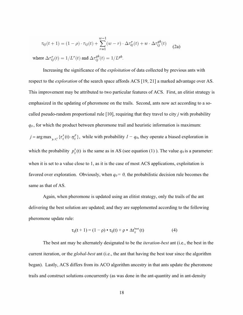
(2a)

Increasing the significance of the exploitation of data collected by previous ants with

respect to the exploration of the search space affords ACS [19, 21] a marked advantage over AS.

This improvement may be attributed to two particular features of ACS. First, an elitist strategy is

emphasized in the updating of pheromone on the trails. Second, ants now act according to a so-

called pseudo-random proportional rule [10], requiring that they travel to city j with probability

q0 , for which the product between pheromone trail and heuristic information is maximum:

while with probability 1 − q0, they operate a biased exploration in

which the probability is the same as in AS (see equation (1) ). The value q0 is a parameter:

when it is set to a value close to 1, as it is the case of most ACS applications, exploitation is

favored over exploration. Obviously, when q0 = 0, the probabilistic decision rule becomes the

same as that of AS.

jarg max (t) ,k

i

kij ijN

j βτ η∈

= ⋅

(t)kijp

Again, when pheromone is updated using an elitist strategy, only the trails of the ant

delivering the best solution are updated; and they are supplemented according to the following

pheromone update rule:

τij(t + 1) = (1 − ρ) • τij(t) + ρ • (4) bestt (t)ij∆

The best ant may be alternately designated to be the iteration-best ant (i.e., the best in the

current iteration, or the global-best ant (i.e., the ant that having the best tour since the algorithm

began). Lastly, ACS differs from its ACO algorithm ancestry in that ants update the pheromone

trails and construct solutions concurrently (as was done in the ant-quantity and in ant-density

18

algorithms). Incidentally, another measure by which ACS encourages exploration as a means of

compensation for the effect of the two modifications described above is to allow erosion of

pheromone upon heavily traveled trails in order to preclude the ant algorithm equivalent of a

traffic jam from occurring. Furthermore, ACS has been augmented with local search routines

which receive the solutions generated by ants and calculate their local optimum values preceding

pheromone update.

MMAS [11] introduces both a constraint of upper and lower bounds to the values of

pheromone available to the ants and a different initialization of these values. Also, MMAS

restricts the range of the pheromone strength to within the interval [τmin , τmax ], and pheromone

trails are initialized to their greatest allowable value, resulting in exploration over a broader

range of potential solutions near the outset of the algorithm. As in ACS, MMAS allows only the

best ant to add pheromone following each iteration of the algorithm. Results indicate that

superior results occur when the global-best ant (as opposed to the iteration-best ant) alternative is

employed with increasing frequency over the course of the algorithm’s execution. Lastly,

MMAS, like ACS, makes use of a local search subroutine in order to optimize its performance in

these smaller regions, or subsets, of the solution space.

19

CHAPTER FOUR: THEORETICAL CONSIDERATIONS

The brief history of the ACO metaheuristic is almost exclusively a history of

experimental research. The process of trial and error has directed most early researchers and still

guides the preponderance of ongoing research efforts. This is the typical situation for virtually

all existing metaheuristics: it is only after experimental work has shown the practical

applications of a new metaheuristic that researchers attempt to extend their understanding of a

metaheuristic’s functioning not only through increasingly complicated experiments but also by

means of an exploration of relevant theory. Often, the initial theoretical problem considered is

one concerning a metaheuristic’s capacity to converge to an optimal solution, followed by

inquiries regarding such topics as the speed of convergence, the effects of the metaheuristic’s

parameters, and the identification of problem characteristics that make success more likely. In

short, given the novelty of the approach and the mathematical intractability of certain

applications, the body of theory surrounding ACO is rather limited. Notwithstanding these

limitations, we discuss the convergence of certain ACO algorithms to optimal solutions and

investigate the relationship between ACO and other well-known techniques. The convergence

proofs presented in the following sections do not apply generally to the metaheuristic, but instead

to those ACO algorithms that are more amenable to theoretical analysis, such as the MAX– MIN

Ant System or the Ant Colony System.

The first theoretical aspect of ACO to be considered in this chapter is the convergence

problem: Will the algorithm find an optimal solution? After all, ACO algorithms are stochastic

search procedures in which bias introduced by the pheromone trails could prevent them from

converging to the optimum. A stochastic optimization algorithm may be assessed according to

20

two kinds of convergence: convergence in value and convergence in solution. Informally,

convergence in value considers the probability that an algorithm will generate an optimal

solution at least once. Convergence in solution, on the other hand, entails evaluating the

probability that an algorithm will attain a state that will continue generating the same optimal

solution. Note that while convergence in solution is more difficult to prove than convergence in

value, from a practical point of view, finding the optimal solution just once will suffice.

Therefore, in this case, convergence in value is all that is needed.

In the following, we define two ACO algorithms called ACO bs,τmin and ACO bs,τmin (Ө), and

we prove convergence results for both of them: convergence in value for ACO algorithms in

ACO bs,τmin (Ө) and convergence in solution for ACO algorithms in ACO bs,τmin (Ө). Here, Θ is the

iteration counter of the ACO algorithm and τmin(Ө) indicates that the tmin parameter may change

during a run of the algorithm. We then show that these proofs continue to hold when typical

elements of ACO, such as local search and heuristic information, are introduced. Finally, we

discuss the significance of these results and demonstrate that the proof of convergence in value

applies directly to two of the most successful ACO algorithms: MMAS and ACS.

Unfortunately, no results are currently available on the speed of convergence of any ACO

algorithm. Therefore, the only way to measure algorithmic performance is to run extensive

experimental tests.

Convergence Proofs

In this section, we study the convergence properties of some important subsets of ACO

algorithms. First, we define the ACObs,τmin algorithm and prove its convergence in value. Next,

21

we define the ACO bs,τmin (Ө) algorithm and prove its convergence in solution. After showing that

both proofs continue to hold when local search and heuristic information are added, we discuss

the meaning of the proofs and determine to which of the ACO algorithms the convergence in

value proof applies.

Consider that, in the ant solution construction procedure, the initial location of each ant is

chosen in a problem-specific way so that Fij(τij) F(τij) [i.e., we remove the dependence of the

function F on the arc (i, j) to which it is applied; this is tantamount to removing the dependence

on the heuristic η. Additionally, in order to facilitate the following derivations, we assume F(τij)

to be of the form used in almost all ACO algorithms: F(τij) = ταij, where 0 < α < + is a

parameter. The probabilistic construction rule applied by the ants to build solutions yields

(5)

Second, the pheromone update procedure is implemented by choosing ŜΘ = sbs (i.e., the

reference set contains only the best-so-far solution) and, additionally, a lower limit τmin > 0 is

imposed upon the value of pheromone trails. In practice, the ACO metaheuristic procedure of

figure 1 becomes the ACO bs,τmin PheromoneUpdate procedure shown in figure 2.

22

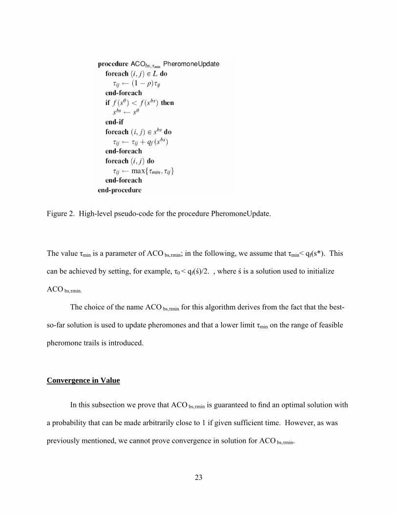
Figure 2. High-level pseudo-code for the procedure PheromoneUpdate.

The value τmin is a parameter of ACO bs,τmin; in the following, we assume that τmin< qf(s*). This

can be achieved by setting, for example, τ0 < qf(ś)/2. , where ś is a solution used to initialize

ACO bs,τmin.

The choice of the name ACO bs,τmin for this algorithm derives from the fact that the best-

so-far solution is used to update pheromones and that a lower limit τmin on the range of feasible

pheromone trails is introduced.

Convergence in Value

In this subsection we prove that ACO bs,τmin is guaranteed to find an optimal solution with

a probability that can be made arbitrarily close to 1 if given sufficient time. However, as was

previously mentioned, we cannot prove convergence in solution for ACO bs,τmin.

23

Before proving the first theorem, it is convenient to show that, due to pheromone

evaporation, the maximum possible pheromone level τmax is asymptotically bounded.

Proposition 1 For any τij it holds that

.max( *)lim ( ) f

ijq sτ τρΘ→∞

Θ ≤ =

Proof The maximum possible amount of pheromone added to any arc (i, j) after any iteration is

qf(s*). Clearly, at iteration 1 the maximum possible pheromone trail is (1 – ρ)τ0 + qf(s*), at

iteration 2 it is (1 – ρ)2τ0 + (1 – ρ)qf(s*) + qf(s*), and so on. Hence, due to pheromone

evaporation, the pheromone trail at iteration Θ is bounded by

max

01

( ) (1 ) (1 ) ( *).ij

if

iq sτ ρ τ ρ

ΘΘ Θ−

=

Θ = − + −∑

As 0 < ρ 1, this sum converges asymptotically to

max( *)fq sτρ

= .

Proposition 2 Once an optimal solution s* has been found, it holds that

** *

,max( )( , ) : lim ( ) f

ijq si j s τ τρΘ→∞

∀ ∈ Θ = =

where *ijτ is the pheromone trail value on connections ( , ) *i j s∈ .

Proof Once an optimal solution has been found, recalling that * *min1, ( )ijτ τ∀Θ ≥ Θ ≥ and that the

best-so-far update rule is used, we have that * ( )ijτ Θ monotonically increases. The proof of

proposition 2 is basically a repetition of the proof of proposition 1, restricted to the connections

24

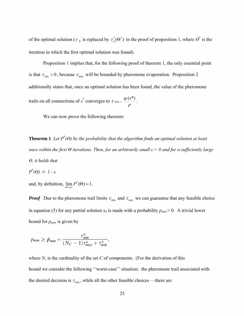
of the optimal solution ( 0τ is replaced by * *( )ijτ Θ in the proof of proposition 1, where Ө* is the

iteration in which the first optimal solution was found).

Proposition 1 implies that, for the following proof of theorem 1, the only essential point

is that min 0τ > , because maxτ will be bounded by pheromone evaporation. Proposition 2

additionally states that, once an optimal solution has been found, the value of the pheromone

trails on all connections of s* converges to max( *)fq sτρ

= .

We can now prove the following theorem:

Theorem 1 Let P*(Ө) be the probability that the algorithm finds an optimal solution at least

once within the first Θ iterations. Then, for an arbitrarily small ε > 0 and for α sufficiently large

Ө, it holds that

P*(Ө) 1 - ε

and, by definition, *lim ( ) 1.PΘ→∞

Θ =

Proof Due to the pheromone trail limits minτ and maxτ we can guarantee that any feasible choice

in equation (5) for any partial solution xh is made with a probability pmin > 0. A trivial lower

bound for pmin is given by

where Nc is the cardinality of the set C of components. (For the derivation of this

bound we consider the following ‘‘worst-case’’ situation: the pheromone trail associated with

the desired decision is minτ , while all the other feasible choices —there are

25

at most Nc - 1—have an associated pheromone trail of maxτ .) Then, any generic

solution ś, including any optimal solution *s S*∈ , can be generated with a probability

, where n < + is the maximum length of a sequence. Because only one ant need

find an optimal solution, a lower bound for

*ˆ ( ) 0ijp Θ >

*( )P Θ is given by

*ˆ ˆ( ) 1 (1 ) .P p ΘΘ = − −

By choosing a sufficiently large Ө, this probability can be made larger than any value

1 - ε. Hence, we have that *ˆlim ( ) 1.PΘ→∞

Θ =

Convergence in Solution

In this subsection we prove convergence in solution for ACObs,τmin (Ө) , which differs

from ACObs,τmin in that it allows a change in value for τmin while solving a problem. That is, we

prove that, in the limit, any arbitrary ant of the colony will construct the optimal solution with

probability 1. This cannot be proved if we impose, as was done in the case of ACObs,τmin , a

small, positive lower bound on the lower pheromone trail limits because at any iteration Ө, each

ant can construct any solution with a nonzero probability. The key to the proof is therefore to

allow the lower pheromone trail limits to decrease over time toward zero, but making this

decrement occur at a sufficiently slow rate to guarantee that the optimal solution is eventually

found. We call ACObs,τmin (Ө) the modification of ACObs,τmin obtained in this way, where τmin(Ө)

indicates the dependence of the lower pheromone trail limits on the iteration counter.

The proof of convergence in solution is organized in two theorems. First, in theorem 2 (in

a way analogous to what was done in the proof of theorem 1), we prove that it can still be

26

guaranteed that an optimal solution is found with a probability converging to 1 when lower

pheromone trail limits of the ACObs,τmin (Ө) algorithm decrease toward 0 at not more than

logarithmic speed (in other words, we prove that ACObs,τmin (Ө) converges in value). Next, in

theorem 3 we prove, under the same conditions, convergence in solution of ACObs,τmin (Ө).

Theorem 2 Let the lower pheromone trail limits in ACObs,τmin (Ө) be

min1, ( )ln( 1)

dτ∀Θ ≥ Θ =Θ+

,

with d being a constant, and let be the probability that the algorithm finds an

optimal solution at least once within the first Θ iterations. Then it holds that

'minˆ ˆ( ) ( ( ))np pΘ ≥ Θ

*lim ( ) 1.PΘ→∞

Θ =

Proof In a manner distinct from what was done in the proof of theorem 1, we prove here that an

upper bound on the probability of not constructing the optimal solution is 0 in the limit (i.e., the

optimal solution is found in the limit with probability 1). Let the event EΘ denote that iteration Θ

is the iteration in which an optimal solution is found for the first time. The event 1 E∞

Θ= Θ∧ ¬ that no

optimal solution is ever found, implies that also one arbitrary, but fixed, optimal solution s* is

never found. Therefore, an upper bound to the probability 1

(P E∞

)ΘΘ=

¬∧ is given by P(s* is never

traversed):

1( ) P(s* is never traversed), P E

∞

ΘΘ=

¬ ≤∧ (6)

Now, in a way similar to what was done in the proof of theorem 1, we can guarantee that at a

generic iteration Θ any feasible choice according to equation (5) can be made with probability

pmin bounded as follows:

27

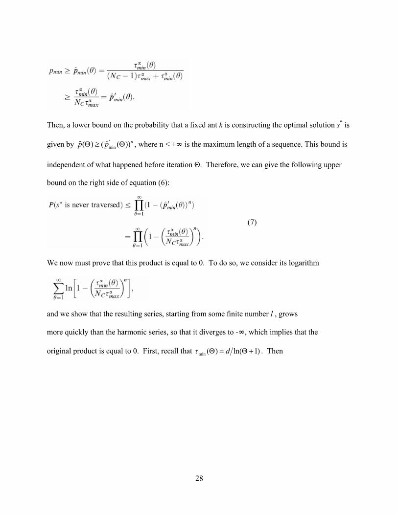
Then, a lower bound on the probability that a fixed ant k is constructing the optimal solution s* is

given by , where n < + is the maximum length of a sequence. This bound is

independent of what happened before iteration Θ. Therefore, we can give the following upper

bound on the right side of equation (6):

'minˆ ˆ( ) ( ( ))np pΘ ≥ Θ

(7)

We now must prove that this product is equal to 0. To do so, we consider its logarithm

and we show that the resulting series, starting from some finite number l , grows

more quickly than the harmonic series, so that it diverges to -, which implies that the

original product is equal to 0. First, recall that min ( ) ln( 1)dτ Θ = Θ+ . Then

28

where 1 mcd d Nαax.τ= .

The inequality holds because for any x < 1, ln(1 – x) -x. The equality holds because

(ln ) ix x −∑ is a diverging series. To see the latter, note that for each positive constant δ > 0 and

for sufficiently large x, (lnx)i δ*x, and therefore δ /(lnx)i 1/x. It then suffices to remember

that 1x x∑ is the harmonic series, which is known to diverge to .

These derivations assert that an upper bound exists for the logarithm of the product given

in equation (7) and, hence, the logarithm on the right side of equation (6) is -.; therefore, the

products given in equation (7) and on the right side of equation (6) must both be 0; in other

words, the probability of never finding the optimal solution 1(P E∞

Θ= )Θ∧ ¬ is 0. Thus, an optimal

solution will be found with probability 1.

In the limiting case, once the optimal solution has been found, we can estimate an

ant’s probability of constructing an optimal solution when following the stochastic

policy of the algorithm. In fact, it can be proved that any ant will in the limit construct the

optimal solution with probability 1—that is, we can prove convergence in solution. Before the

29

proof of this assertion, it is convenient to show that the pheromone trails of connections that do

not belong to the optimal solution asymptotically converge to 0.

Proposition 3 Once an optimal solution has been found and for any ( )ijτ Θ such that *( , )i j s∉ ,

it holds that

*lim P(s , , k ) 1.Θ→∞

Θ =

Proof After the optimal solution has been found, connections not belonging to the optimal

solution no longer receive pheromone. Thus, their value can only decrease. In particular, after

one iteration, , after two iterations,

, and so on (Θ* is the iteration in which s* was first

found). Additionally, we have that

* *min( 1) max ( ), (1 ) ( )ij ijτ τ ρΘ + = Θ − Θ*τ

2 *τ* *min( 2) max ( ), (1 ) ( )ij ijτ τ ρΘ + = Θ − Θ

*lim ln( 1) 0dΘ→∞

Θ +Θ+ = and *lim(1 ) ( ) 0ijρ τΘΘ→∞

− Θ +Θ = .

Therefore, . *lim ( ) 0ijτΘ → ∞ Θ +Θ =

Theorem 3 Let Θ* be the iteration in which the first optimal solution has been found and

P(s*, Θ, k ) be the probability that an arbitrary ant k constructs s* in the Θth iteration, with

Θ > Θ*. Then it holds that

*lim P(s , , k ) 1.Θ→∞

Θ =

Proof Let ant k be located on component i and (i, j) be a connection of s*. A lower bound

for the probability that ant k makes the ‘‘correct choice’’ (i, j) is given by the term *ˆ ( )ijp Θ * ( )ijp Θ

Because of propositions 2 and 3 we have

30

Hence, in the limit, any fixed ant will construct the optimal solution with probability 1 because at

each construction step, it makes the correct decision with probability 1.

Further Considerations

Many ACO algorithms include some features that are present neither in ACObs,τmin nor in

ACObs,τmin (Ө). The most important among them are the use of local search algorithms to improve

the solutions constructed by the ants and the use of heuristic information in the choice of the next

component. Therefore, a natural question to consider is how these features affect the

convergence proof for ACObs,τmin . Note that here and in the following, because remarks made

about ACObs,τmin typically also apply to ACObs,τmin (Ө), we often refer only to ACObs,τmin .

Let us first consider the use of local search. Local search tries to improve an ant’s

solution s by iteratively applying small, local changes to it. Typically, the best solution found

by the local search is returned and used to update the pheromone trails. It is rather easy to see

that the use of local search neither affects the convergence properties of ACObs,τmin , nor those of

ACObs,τmin (Ө). In fact, the validity of both convergence proofs depends only on the way solutions

are constructed and not on the fact that the solutions are taken or not to their local optima by a

local search routine.

's

31

Available a priori information concerning the problem can be used to derive heuristic

information that biases the probabilistic decisions to be made by the ants. When incorporating

such heuristic information into ACObs,τmin , the most common choice is ( ) [ ] [ ]ij ij ij ijF α βτ τ η= . In

this case equation (5), becomes

1 ( , )

[ ] [ ], ( , ) ;

[ ] [ ]( )

0,

ki

ij ij ki

ij ijh h i l

if i jP c j x

otherwise

α β

α β

τ ητ ηΤ + ∈Ν

⎧∈Ν⎪

= = ⎨⎪⎩

∑

where ηij measures the heuristic desirability of adding solution component j. In fact, neither

theorem 1 nor theorems 2 and 3 are affected by the heuristic information if we have

0 < ηij < + for each (i, j)L and ß < . Given these assumptions, η is limited to some

(problem-specific) interval [ηmin, ηmax], with ηmin > 0 and ηmax < +. Then, the heuristic

information simply has the effect of changing the lower bound on the probability pmin of making

a specific decision.

Summary

It is instructive to reflect upon what theorems 1 through 3 really tell us. First, theorem 1

expresses that when using a fixed positive lower bound on the pheromone trails, ACObs,τmin is

guaranteed to find the optimal solution. Theorem 2 extends this result by saying that we

essentially can keep this property for ACObs,τmin (Ө) algorithms, if we decrease the bound τmin to 0

slowly enough. (Unfortunately, theorem 2 cannot be proved for the exponentially fast decrement

of the pheromone trails obtained by a constant pheromone evaporation rate, which most ACO

algorithms use.) However, the proofs say nothing about the time required to find an optimal

32

solution, which can be prohibitively long. A similar limitation applies to other well-known

convergence proofs, such as those formulated for simulated annealing by Hajek (1988) and by

Romeo & Sangiovanni-Vincentelli (1991). Finally, theorem 3 shows that a sufficiently slow

decrement of the lower pheromone trail limits leads to the effect that the algorithm converges to

a state in which the ants repeatedly construct the optimal solution. In fact, for this latter result it

is essential that in the limit the pheromone trails go to 0. If, as is done in ACObs,τmin , a fixed

lower bound τmin is set, it can only be proved that the probability of constructing an optimal

solution is larger than , where min maxˆ1 ( , ε τ τ− ) ε is a function of τmin and τmax . Because in

practice we are more interested in finding an optimal solution at least once than in generating it

again and again, we should take a closer look at the role played by τmin and τmax in the proof of

theorem 1: the smaller the ratio τmax / τmin, the larger the lower bound minp given in the proof.

This is important because the larger the minp , the smaller the worst-case estimate of the number

of iterations Θ needed to assure that an optimal solution is found with a probability larger than

the quantity 1 - ε. In fact, the most restrictive bound is obtained if all pheromone trails are the

same; that is, for the case of uniformly random solution construction. In this case, we would

have minˆ 1/ cp N= (note that this fact is independent of the proximity of the lower bound used in

theorem 1). This somewhat counterintuitive result is due to the fact that our proof is based on a

worst-case analysis; we need to consider the worst-case situation in which the bias in the solution

construction introduced by the pheromone trails is counterproductive and leads to suboptimal

solutions. In other words, we have to assume that the pheromone level associated with the

connection an ant needs to pass in order to construct an optimal solution is τmin, while on the

other connections, it is much higher—in the worst case corresponding to τmax. In practice,

33

however, as shown by the results of many published experimental works, this does not happen,

and the bias introduced by the pheromone trails does indeed help to hasten convergence to an

optimal solution.

34

CHAPTER FIVE: EVOLUTIONARY COMPUTING/ACO HYBRIDS

Having introduced the ACO metaheuristic and reviewed its operation from both a

theoretical and a practical perspective, we may now address the first of the issues enumerated in

the introduction, which will be presented here as a critique of the appropriateness of the

hybridization of evolutionary computing (as well as the closely related family of genetic

algorithms) and ACO from the perspective of biological theory. Unfortunately, in light of the

mathematically intractable nature of problem, the argument for a closer review of the suitability

of combining these two metaheuristics is conducted as follows: First, the mechanism of natural

selection as it is broadly implemented in evolutionary computing is contrasted with the most

modern theories of ant ecology. Second, an assessment of two ACO algorithm’s, one being a

hybridization of a conventional evolutionary algorithm and ACO and the other a hybridization

that more accurately reflects the relevant biological principles, will be conducted. Specifically,

each will be tasked with identical Steiner tree construction problems in order that their relative

performance may be evaluated. A prerequisite to the preceding goals, however, is a better

understanding of certain evolutionary computing principles.

A Primer on Evolutionary Programming and Genetic Algorithms

Evolutionary Programming (EP), as the name implies, mimics evolutionary biology.

Using natural selection as a metaphor, EP looks upon generations of a species and its competitors

within a particular ecological niche as solutions for occupying that niche. EP submits the notion

that solutions, which in this case would be analogous to parents, may be mutated to produce new

more viable solutions as their offspring. Within Genetic Algorithms (GA), the fundamental

35

agents are best compared to individual organisms, whereas in EP, that role would fall to the

algorithms equivalent of a species of animal. The evolution of a solution (i.e., a species) into

progressively improved solutions is realized by the EP model according to the following process:

1. A set of finite automata is randomly generated to represent a population of solutions.

This may be regarded as the first group of parents—a veritable Adam and Eve, if you

will.

2. Each of the solutions is copied into a new population of offspring, wherein a mutation

operator that alters the behavior of the individuals in the new population is applied.

The behavior of each of the offspring is compared to that of its parent in order to

generate a distribution of changes that best addresses the problem at hand.

3. Each individual is then assessed for fitness. Fitness may be evaluated against a

variety of criteria (the ability to recognize a particular input sequence, for example).

A percentage of the individuals deemed most fit are selected to serve as the next

generation of parents.

Steps 2 and 3 continue until a set of finite automata demonstrate the capacity to attain the

prescribed goal.

Evolutionary Programming is conceptually similar to Genetic Algorithms, with the

following notable exceptions: First, EP takes note of the ways in which the behavioral qualities

of parents and their offspring differ, whereas GA’s usually represent individual solutions as

vectors or strings. Interjecting the biological metaphor momentarily, EP functions in the domain

of the phenotype, while GA operates in the domain of the genotype. In the case of EP, the

36

structure of the genes is not considered; rather, it is their impact on the behavior of the proverbial

creature, or automaton, that is of interest.

Second, EP represents mutation differently than GA. An EP mutation operator is defined in such

a way that it favors mutations that generate behavioral distributions of small rather than large

variance. Additionally, as the algorithm progresses and good solutions begin to evolve, the

mutation operator creates distributions of progressively smaller variances.

Both EP and GA are useful methods for problems of optimization. EP is particularly

useful for combinatorial optimization, especially when there are a multitude of potential

solutions as opposed to a single global solution. The matter of their utility when combined with

ACO is addressed in the following section.

Evolution and the Ant

None other than perhaps the most preeminent of entomologists (or more specifically,

myrmecologists), Edward O. Wilson, has shown that natural selection operates upon the social

ants at the colony level [16]. The colony is selected as a whole, and its members contribute to

colony fitness rather than to individual fitness. Indeed, Wilson characterizes the extremely rare

and inconsequential occurrence of individual selection among such ants as a dissolutive force.

Consequently, insofar as a computing discipline appropriates natural selection as a metaphor

with respect to the behavior of ants, the particular means by which the phenomenon of natural

selection imposes itself in the case of the ant would seem an integral (and perhaps, essential)

component in any model thusly derived. In that both Evolutionary Computing and Genetic

37

Algorithms employ selection at the level of the individual, any combination of either of these

two metaheuristics with ACO raises the question of their compatibility.

It is this question of compatibility that is addressed in the following section. Regrettably,

it is not a question that lends itself to rigorous mathematical analysis. Such an analysis, if

possible, would likely shed light upon the matter. Instead, this matter of compatibility is

addressed in a qualitative fashion, using the aforementioned task of Steiner tree construction as

an admittedly imprecise measure of the relative qualities of two solutions: one from a hybridized

EC/ACO algorithm and the other from an ACO algorithm that implements a procedure

analogous to colony-level selection. The latter is a program developed by the author in Matlab.

Broadly speaking, it pits colonies of ants in competition against one another, the most fit of

which (with a colony’s fitness assessed by the collective quality of its solutions) survive to send

some number of queens (each bearing a uniquely mutated version of the genetic character of the

original colony’s queen) to locations in the solution space that have previously shown promise.

Results

Each of the aforementioned programs was presented with identical tasks. A constellation

of random points was generated, with a subset of these points selected (again, randomly) to be

the nodes of a Steiner tree. The cost upon which both algorithms based the relative worth of

potential solutions was simply the sum of the lengths of the branches, or segments connecting

the nodes of the Steiner tree. Both programs proposed reasonable solutions that appear

comparable in quality. A more precise comparison of their performance would offer little more

in the way of conclusions as there are significant differences between them other than their

38

disparate implementations of the evolution metaphor. However, the viability of the algorithm

incorporating selection at the colony-level appears to have been confirmed. Figure 2 displays a

typical result.

Figure 3. Steiner tree solution generated by Matlab ACO with colony-level selection.

39

CHAPTER SIX: CONCLUSIONS

Despite the critical tenor of this review, there is no denying ACO’s successful

exploitation of stigmergy (i.e., the term describing the ants’ indirect, pheromone-based mode of

communication) as a computing tool of significant potential. However, the possibility that

daemon actions may exert a dissolutive influence (similar to that of the potential misapplication

of evolutionary theory considered in the last chapter) upon a paradigm that is fundamentally one

of decentralized control warrants further investigation. Though inclusion of such global controls

in ACO has undoubtedly yielded net improvement, a cursory examination admits the possibility

that they may suppress in some measure the densely heterarchical dynamic observed among ants

in a colony. A definitive answer is more likely to be found analytically. The latter of these two

approaches had been the primary goal of this exercise, though it is one that will have to be

addressed at some future date for reasons stated previously.

40

LIST OF REFERENCES

[1] Alupoaei S, Katkoori S. Ant colony system application to marcocell overlap removal.

IEEE Trans Very Large Scale Integr (VLSI) Syst

2004;12(10):1118-22.

[2] Bautista J, Pereira J. Ant algorithms for assembly line balancing. In: Dorigo M, Di Caro

G, Sampels M, editors. Ant algorithms—Proceedings

of ANTS 2002—Third international workshop. Lecture Notes in Comput Sci, vol. 2463.

Berlin: Springer; 2002. p. 65-75.

[3] Bertsekas DP, Tsitsiklis JN, Wu C. Rollout algorithms for combinatorial optimization. J

Heuristics 1997;3:245-62.

[4] Bianchi L, Gambardella LM, Dorigo M. An ant colony optimization approach to the

probabilistic traveling salesman problem. In: Merelo JJ,

Adamidis P, Beyer H-G, Fernández-Villacanas J-L, Schwefel H-P, editors. Proceedings

of PPSN-VII, seventh international conference on parallel problem solving from nature.

Lecture Notes in Comput Sci, vol. 2439. Berlin: Springer; 2002. p. 883-92.

[5] Bilchev B, Parmee IC. The ant colony metaphor for searching continuous design spaces.

In: Fogarty TC, editor. Proceedings of the AISB workshop on evolutionary computation.

Lecture Notes in Comput Sci, vol. 993. Berlin: Springer; 1995. p. 25-39.

[6] Birattari M, Di Caro G, Dorigo M. Toward the formal foundation of ant programming.

In: Dorigo M, Di Caro G, Sampels M, editors. Ant algorithms—Proceedings of ANTS

2002—Third international workshop. Lecture Notes in Comput Sci, vol. 2463. Berlin:

Springer; 2002. p. 188-201.

41

[7] Blesa M, Blum C. Ant colony optimization for the maximum edge-disjoint paths

problem. In: Raidl GR, Cagnoni S, Branke J, Corne DW, Drechsler R, Jin Y, Johnson

CG, Machado P, Marchiori E, Rothlauf R, Smith GD, Squillero G, editors. Applications

of evolutionary computing, proceedings of EvoWorkshops 2004. Lecture Notes in

Comput Sci, vol. 3005. Berlin: Springer; 2004. p. 160-9.

[8] Blum C. Beam-ACO—Hybridizing ant colony optimization with beam search: An

application to open shop scheduling. Computers & Operations Res 2005;32(6):1565-91.

[9] Bullnheimer B, Hartl R, Strauss C. A new rank-based version of the Ant System: A

computational study. Central European J Operations ResEconom 1999;7(1):25-38.

[10] Campos M, Bonabeau E, Theraulaz G, Deneubourg J-L. Dynamic scheduling and

division of labor in social insects. Adapt Behavior 2000;8(3):83-96.

[11] Corry P, Kozan E. Ant colony optimisation for machine layout problems. Comput Optim

Appl 2004;28(3):287-310.

[12] Duin C, Voß S. The pilot method: A strategy for heuristic repetition with application to

the steiner problem in graphs. Networks 1999;34(3):181-91.

[13] Gagné C, Price WL, Gravel M. Comparing an ACO algorithm with other heuristics for

the single machine scheduling problem with sequence dependent setup times. J Oper Res

Soc 2002;53:895-906.

[14] Handl J, Knowles J, Dorigo M. Ant-based clustering and topographic mapping. Artificial

Life 2006;12(1). In press.

[15] Hoos HH, Stützle T. Stochastic local search: Foundations and applications. Amsterdam:

Elsevier; 2004.

42

[16] Karpenko O, Shi J, Dai Y. Prediction of MHC class II binders using the ant colony search

strategy. Artificial Intelligence in Medicine 2005;35(1-2):147-56.

[17] Kennedy J, Eberhart RC. Particle swarm optimization. In: Proceedings of the 1995 IEEE

international conference on neural networks, vol. 4. Piscataway, NJ: IEEE Press; 1995.

p. 1942-8.

[18] Michel R, Middendorf M. An island model based ant system with lookahead for the

shortest supersequence problem. In: Eiben AE, Bäck T, Schoenauer M, Schwefel H-P,

editors. Proceedings of PPSN-V fifth international conference on parallel problem

solving from nature. Lecture Notes in Comput Sci, vol. 1498. Berlin: Springer; 1998.

p. 692-701.

[19] Nemhauser GL, Wolsey AL. Integer and combinatorial optimization. New York: John

Wiley & Sons; 1988.

[20] Ow PS, Morton TE. Filtered beam search in scheduling. Internat J Production Res

1988;26:297-307.

[21] Papadimitriou CH, Steiglitz K. Combinatorial optimization—Algorithms and complexity.

New York: Dover; 1982.

[22] Parpinelli RS, Lopes HS, Freitas AA. Data mining with an ant colony optimization

algorithm. IEEE Trans Evolutionary Comput 2002;6(4):321-32.

[23] Reeves CR, editor. Modern heuristic techniques for combinatorial problems. New York:

John Wiley & Sons; 1993.

[24] Reimann M, Doerner K, Hartl RF. D -ants: Savings based ants divide and conquer the

vehicle routing problems. Comput Oper Res

2004;31(4):563-91.

43

[25] Shmygelska A, Aguirre-Hernández R, Hoos HH. An ant colony optimization algorithm

for the 2D HP protein folding problem. In: Dorigo M,Di Caro G, Sampels M, editors. Ant

algorithms—Proceedings of ANTS 2002—Third international workshop. Lecture Notes

in Comput Sci, vol. 2463. Berlin: Springer; 2002. p. 40-52.

44