A Comparative General Equilibrium Analysis of the …€¦ · 28 A Comparative General Equilibrium Analysis of the Estonian Labour Market Alari Paulus Andres Võrk Kari E. O. Alho

28

A Comparative General Equilibrium Analysis

of the Estonian Labour Market

Alari Paulus Andres Võrk

Kari E. O. Alho (ETLA)

This paper analyses the impact of several tax-benefit reforms on the employment of different skill groups under various wage formation systems. We adapt a general equilibrium model initially developed for the Finnish economy by Alho (2006), combining it with elements from Bovenberg et al. (2000) and Hinnosaar (2004a, b). Policy simulations demonstrate the importance of wage setting for the outcome. In the case of Estonia, market determined wages outperform bargained wages, which could imply an important difference between the EU-15 countries and the new member states in general. Additionally, the labour supply of the low-skilled is most effectively increased by lowering the marginal income tax rate, which combined with strategies increasing the overall employment, could potentially improve the labour market position of those with lower skills.

This is a part of the project “Tax/benefit systems and growth potential of the EU” (TAXBEN, Project no. SCS8-CT-2004-502639), financed by the European Commission under FP 6 of Research. Keywords: computable general equilibrium models, labour tax policy, wage structure

JEL classification: D58, E62, J31

January 2007

PRAXIS Working Papers No 28/2007

2

A COMPARATIVE GENERAL EQUILIBRIUM ANALYSIS OF THE ESTONIAN LABOUR MARKET∗

Alari Paulus, PRAXIS

Andres Võrk, PRAXIS

Kari E. O. Alho, ETLA

Abstract: This paper analyses the impact of several tax-benefit reforms on the

employment of different skill groups under various wage formation systems. We adapt a

general equilibrium model initially developed for the Finnish economy by Alho (2006),

combining it with elements from Bovenberg et al. (2000) and Hinnosaar (2004a, b).

Policy simulations demonstrate the importance of wage setting for the outcome. In the

case of Estonia, market determined wages outperform bargained wages, which could

imply an important difference between the EU-15 countries and the new member states

in general. Additionally, the labour supply of the low-skilled is most effectively

increased by lowering the marginal income tax rate, which combined with strategies

increasing the overall employment, could potentially improve the labour market

position of those with lower skills.

Keywords: computable general equilibrium models, labour tax policy, wage structure

JEL classification: D58, E62, J31

Corresponding author:

Andres Võrk PRAXIS Center for Policy Studies Estonia pst 5a, Tallinn 10143, Estonia e-mail: [email protected]

∗ This is a part of the project “Tax/benefit systems and growth potential of the EU” (TAXBEN, Project no. SCS8-CT-2004-502639), financed by the European Commission under FP 6 of Research. We thank Karsten Staehr and all the seminar participants at CPB for helpful comments. All remaining errors are ours.


3

Contents

1. Introduction .............................................................................................................. 4

2. The model ................................................................................................................. 7

2.1. Households ....................................................................................................... 7

2.2. Firms................................................................................................................. 8

2.3. Wage formation .............................................................................................. 10

2.4. Government .................................................................................................... 11

3. Calibration .............................................................................................................. 12

4. Policy simulations .................................................................................................. 14

4.1. Description ..................................................................................................... 14

4.2. Lowering the marginal income tax rate.......................................................... 16

4.3. Increasing the income tax allowance.............................................................. 17

4.4. Lowering employers’ social security contributions ....................................... 17

4.5. Increasing the replacement rate ...................................................................... 18

5. Conclusions ............................................................................................................ 19

References ...................................................................................................................... 20

Appendices ..................................................................................................................... 21

Appendix 1. A comparison of CGE models ............................................................... 21

Appendix 2. Labour supply ........................................................................................ 26

Appendix 3. Labour cost ............................................................................................ 27

Appendix 4. Wage bargaining.................................................................................... 28


4

1. Introduction

The European Union countries are increasingly concerned about their competitiveness

in the global market. One of the central issues is related to the functioning of the labour

market and social protection systems. In frequent comparisons of the US and the EU

labour market, the latter has been considered more regulated and rigid, which again has

been associated with higher unemployment rates. On the other hand, labour in Europe

enjoys higher social protection standards. Under the pressure of global processes,

current trends are towards adjustments in tax-benefit systems, which could increase

work incentives and improve flexibility of labour market without scaling back social

protection too much (Carone and Salomäki, 2001). Also the re-launched Lisbon

Strategy and the underpinning integrated guidelines advocate more employment

friendly tax-benefit systems.

The enlargement of the EU in 2004 introduced new member states, which, having

relatively decentralised labour markets, also contrast with the EU-15 countries. There

are some concerns that this could lead to social dumping. In this context, the new

member states have a dilemma as to which way to proceed – continuing the market-

oriented flexible approach or shifting to a more centralised bargaining and protective

system. There is some empirical evidence that a bell-shaped relationship exists between

the centralisation of wage bargaining and the unemployment level (Calmfors and

Driffill, 1988), possibly making choices in-between relatively unfavourable.

In this paper we take Estonia as one example of the new member states and try to

answer whether it would be beneficial to implement a tax-benefit system more akin to

those found in the old EU countries. Estonia is a small open economy conducting liberal

economic and tax policy. Recent and on-going tax-benefit reforms aimed at lowering

the income tax burden and to increase unemployment and subsistence benefits represent

a good opportunity to model the outcome under various wage formation hypotheses.

We adopt a computable general equilibrium (CGE) model initially developed for

Finnish economy as a part of the TAXBEN project, see Alho (2006), but also with

elements from the models of Bovenberg et al. (2000) for Dutch and Hinnosaar (2004a,

b) for Estonian economy.


5

The main features of the model are the following. There are two production factors –

capital and labour, the latter divided further into three skill groups based on educational

attainment. Firms are symmetric and produce one homogenous good. The goods market

is characterised by monopolistic competition, implying positive profits for firms. The

foreign sector is not explicitly modelled, domestic firms compete with foreign firms in

the international market and it is assumed that the domestic price level of goods equals

the international price level. Households earn labour income, receive distributed profits

and unemployment benefits. Their utility depends on leisure, private consumption, on

which all the income is spent, and public consumption. Government has a passive role

of spending all tax income on unemployment benefits and public consumption. Tax

revenue is generated by income taxes on labour and capital and employers’ social

security contributions. Throughout the model, functions with constant elasticity of

substitution (CES) have been used (e.g. for production, aggregation of production

factors, utility).

Three different structures of wage formation are modelled. First, fixed wages, which in

case of a tax-benefit policy change would reflect the first reaction in the (very) short

run. Second, market determined wages, which may correspond to the Estonian case

under current circumstances in the medium run. (We do not consider the long run as

capital is held fixed.) Third, wage bargaining by each skill group, representing a more

EU-oriented hypothetical case.

Overall, labour supply and wage bargaining are modelled in the manner of Bovenberg et

al. (2000) and Hinnosaar (2004a, b), while the production side and other wage

formation schemes (fixed and market determined) are modelled as in Alho (2006). A

more detailed comparison of the previous models and the current approach is presented

in Appendix 1.

General equilibrium effects of Estonian tax-benefit system have not been extensively

researched. To our knowledge, there are no previous studies apart from Hinnosaar

(2004a, b). Compared to the latter, we consider several alternative wage formation

systems. We also introduce capital as a production factor, although fixed, and employ

more recent data. Additionally, having available a similar model to the Finnish case

allows to compare tax-benefit effects on employment in an old and a new member state,


6

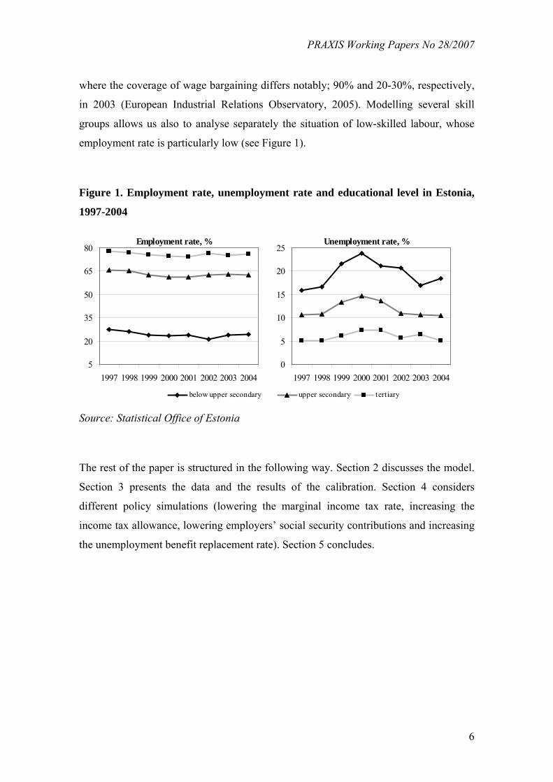
where the coverage of wage bargaining differs notably; 90% and 20-30%, respectively,

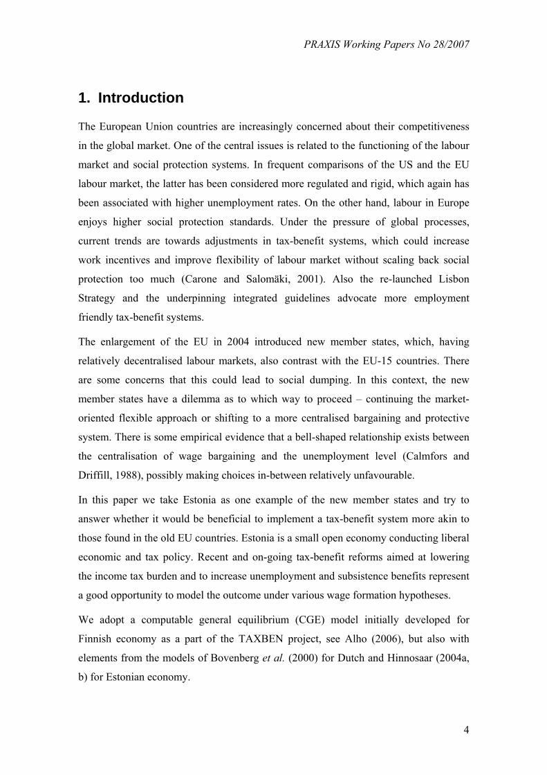
in 2003 (European Industrial Relations Observatory, 2005). Modelling several skill

groups allows us also to analyse separately the situation of low-skilled labour, whose

employment rate is particularly low (see Figure 1).

Figure 1. Employment rate, unemployment rate and educational level in Estonia,

1997-2004

Employment rate, %

5

20

35

50

65

80

1997 1998 1999 2000 2001 2002 2003 2004

below upper secondary

Unemployment rate, %

0

5

10

15

20

25

1997 1998 1999 2000 2001 2002 2003 2004

upper secondary tertiary

Source: Statistical Office of Estonia

The rest of the paper is structured in the following way. Section 2 discusses the model.

Section 3 presents the data and the results of the calibration. Section 4 considers

different policy simulations (lowering the marginal income tax rate, increasing the

income tax allowance, lowering employers’ social security contributions and increasing

the unemployment benefit replacement rate). Section 5 concludes.


7

2. The model

2.1. Households1

The workforce consists of three types of households differing in skills based on

educational attainment: low-skilled, skilled and high-skilled ( 3,2,1=i ). There are Mi

households in each skill category who maximise utility subject to a budget constraint

and a time constraint. The utility of household j with skill level i is a function of private

consumption jiC , leisure j

iV and public consumption G . The latter enters in an

additively separable way, therefore having no effect on labour supply decisions2:

)(),( GgVChH ji

ji

ji += (1)

The utility sub-function is the CES type:

( ) ( ) ( ) 11111

1),(−−−

⎥⎦

⎤⎢⎣

⎡−+=

δδ

δδ

δδδ

δ jii

jii

ji

ji VdCdVCh (2)

where δ is the elasticity of substitution between consumption and leisure and di is a

distribution parameter implying the relative weights which households place on

consumption and labour supply. A household’s budget constraint is

ji

jii

Li PCSWt =− )1( (3)

where Lit is the average tax rate on labour income (a function of labour income, tax

rates and tax free allowance), Wi is the gross wage rate, jiS is labour supply and P is the

price level. Households also receive capital income from distributed profits, however it

is assumed that they are not able to anticipate it ex ante and therefore it does not enter

the budget constraint here. The time endowment is normalised to unity, ji

ji VS −=1 , i.e.

the unit of time endowment (and labour supply) could be considered as a full-time job.

1 This section follows Bovenberg et al. (2000) and Hinnosaar (2004a, b). However, there is an important difference in the aggregate labour supply equation. See Appendix 2 for the details.

2 The utility from public consumption for a skill group is derived as GgdGg ii1

1

)( −= δ , where gi is the share of the skill group in public consumption. The latter is an exogenous variable.


8

The total labour supply of skill group i is Mi times the labour supply jiS of one

household:

( )

( ) ( ) δ

δ

−

−

⎟⎠⎞

⎜⎝⎛ −−

−+

⎟⎟⎠

⎞⎜⎜⎝

⎛⎟⎠⎞

⎜⎝⎛ −−

−

=

PWm

PddWm

PWm

PddmTM

Si

i

ii

i

i

iAi

i 11111

1111 (4)

where m is marginal tax rate on labour income and TA is the tax allowance. Households

decide the optimal amount of labour supply, however, the participation decisions are

exogenous. Total labour supply Si of skill group i implies that in the end Si households

from that skill group are supposed to supply all their labour in the model and the rest are

considered as inactive.

In this framework firms decide employment Ei, which therefore equals the labour

demanded Ni. Some households are unemployed and receive instead of labour earnings

unemployment benefits Bi (also taxed). Aggregate (realised) private consumption C is

equal to labour income, unemployment benefits and capital income, all net of taxes:

( ) ( )[ ] ( )∑ Π−+−+−=i ii

Biii

Li mUBtEWtPC 111 (5)

where Ui is the number of unemployed (also corresponding to full-time jobs) and Π is

aggregate capital income. Note that the marginal tax rate is constant and not dependent

on income type or skill group. In fact, all income is taxed in a common framework and

tax allowance is in principle applied to total income. However, it is assumed that the tax

allowance is assigned to either labour income or unemployment benefits and both

exceed that, so that any additional income, i.e. capital income, must be taxed in full

extent. The different average tax rates for labour income and unemployment benefits are

due to the different underlying amounts.

2.2. Firms

This section is based on Alho (2006). There is monopolistic competition in the economy

between identical firms. Firms use two aggregate production inputs – capital and labour

– to produce one homogenous good. The aggregate production function is a CES

function implying constant returns to scale:


9

[ ]σσσ αα1

)1( LKAQ −+= (6)

where A is total factor productivity, K capital stock, L aggregate effective labour input,

α a distribution parameter and )1(1 σ− the substitution elasticity between capital and

aggregate effective labour.

The aggregate demand Q* in the international market depends on the international price

level ε−∗∗ = )(, PbQP D , where 0>ε . Firms maximise profits, which assuming Cournot

competition leads to the demand for effective labour input:

( )LCQQQ

PQ

dQdPP L =⎟⎟

⎠

⎞⎜⎜⎝

⎛+∗∗

∗

∗

∗∗ 1 (7)

where QL is the marginal productivity of aggregate labour, hQQ =∗ the market share

of domestic firms and ( )LC is the aggregate unit labour cost. This can be rewritten as:

( ) ( )LCQhP L =− −∗ 11 ε (8)

where ( )11 −− εh is the inverse of the mark-up. This determines the employment. The

capital stock remains fixed as we concentrate only on the short-medium run.

Aggregate effective labour input L is a CES aggregate of labour demanded in each skill

group Ni:

( )[ ] 1,1

≤= ∑ φφφi ii NeL (9)

Here, ei is the relative efficiency/productivity parameter of the skill group i with e1 fixed

to unity and )1(1 φ− is the substitution elasticity of skill groups. The gross wage rate is

Wi, but the corresponding cost to the employer, i.e. the producer wage, is

ii WvNC )1()( += , where v is the rate of employers’ compulsory social security

contribution. Setting up and solving a cost minimisation problem gives us the relative

demand for the different skill groups (see Appendix 3 for the derivation):

( )( )

1

111

−

⎟⎟⎠

⎞⎜⎜⎝

⎛⎟⎟⎠

⎞⎜⎜⎝

⎛=

φφ

NN

ee

NCNC iii , i = 2, 3 (10)

and the aggregate unit labour cost:


10

( ) ( )φφ

φφ

−−

−−

⎥⎥⎥

⎦

⎤

⎢⎢⎢

⎣

⎡

⎟⎟⎠

⎞⎜⎜⎝

⎛= ∑

1

1

ii

i

eNC

LC (11)

2.3. Wage formation

Similarly to Alho (2006) we consider several wage formation hypotheses. First, fixed

wages reflecting the first reactions in the (very) short run after a tax-benefit policy

change. Second, market determined wages corresponding to a flexible labour market

with market clearing in the medium run (capital still fixed). Third, we consider a case of

wage bargaining. The first two settings are perhaps closer to the actual situation in the

Estonian labour market within the respective time horizon; the last one is somewhat

more hypothetical, reflecting the old EU member states.

The case of fixed wages is the easiest to model, requiring only the relevant constraint in

the model. Market determined wages need an additional restriction related to

unemployment, which otherwise would not exist in the model. Here, unemployment

rates have been fixed under market determined wages. Bargained wages are determined

by a right-to-manage model, which is as follows, being a combination of approaches by

Hinnosaar (2004a, b) and Alho (2006).

The employers’ organisation and three unions each representing workers of one skill

group bargain over wages and employers determine employment. This implies

maximising the following Nash function:

iiii

ββ −ΓΛ=Ω 1 (12)

where

( ) KdEWvLKPQi ii )(1),( +−+−=Λ ∑ ρ (13)

and

( ) ( )[ ] 5.05.0 11 iBii

Liii BtWtE −−−=Γ (14)

Λ stands for the total profit of the employers’ organisation and Γi represents the utility

of the union; ρ denotes the rate of return on capital and d the depreciation rate. It is

assumed that the union attaches equal weight to employment and the surplus from


11

working, i.e. the real consumer wage less the reservation wage what is simply the after-

tax unemployment benefit. The parameter βi denotes the relative bargaining power of

the employers. Solving the Nash function gives the following wage equation of skill

group i (see Appendix 4 for the derivation):

( )( ) ( )[ ]

( ) ( )ii

ij jji

i

iii Ev

KdEWvLKQPBW

β

ρβ

ββ

++

+−+−−+

+=

∑ ≠∗

11

)(1),(1

15.0 (15)

Note that bargained wages do not depend on the marginal tax rate. This is due to the fact

that wages and benefits are taxed in the same manner, applying the same marginal tax

rate and tax allowance. This implies that if the employers’ organisation dictates the

outcome, 1=iβ , the wage is suppressed down to the reservation wage, i.e. the

unemployment benefit, ii BW = . In case a labour union dominates the bargaining,

0=iβ , all the production surplus is attributed to wage income:

( )( ) i

ij jji Ev

KdEWvLKQPW

+

+−+−=

∑ ≠∗

1

)(1),( ρ (16)

2.4. Government

The government runs a balanced budget, spending collected tax revenues on

unemployment benefits and public consumption. There is a universal income tax

applied on all income, including unemployment benefits, with constant marginal tax

rate. Yet, income taxation is progressive due to income tax allowance. It is applied to

either labour earnings or benefits, depending on which of these a household is receiving,

which are assumed to be sufficiently large so that the tax allowance could be utilised

fully. Therefore, the rest of the income, namely capital income in the form of distributed

corporate profits, is subject to full taxation. The average tax rate on labour earnings

could be denoted as

( )i

AiL

i WTWm

t−

= (17)

and the average tax rate on unemployment benefits as


12

( )i

AiB

i BTBm

t−

= (18)

where TA is the amount of tax allowance. Additionally, there is a compulsory social

security contribution on employers with a constant rate of v. No value-added tax is used.

Government uses its resources to finance unemployment benefits and the rest is spent

on public consumption. Unemployment benefits are indexed to the gross wage rate,

ii rWB = , where r is the pre-tax replacement rate. Overall, the government budget is:

[ ] PGmUBtEWtvi ii

Biii

Li =Π+−−+∑ )1()( (19)

3. Calibration

The model has been calibrated to the Estonian economy in 2004. Input data and

parameters are shown in Table 1. Labour market data and gross wage rates have been

derived from the Labour Force Survey (Statistical Office of Estonia, 2004). There is a

population of 830.1 thousand of persons in working age (16 to pension age). This is

divided into three skill groups based on educational level (below upper secondary,

upper secondary and tertiary): low-skilled, skilled and high-skilled. Labour force

participation rates across the skill groups are, respectively, 42.4%, 76.6% and 88.2%,

and unemployment rates 20.8%, 11.0% and 5.4%. The gross wage rate for skilled and

high-skilled is higher by respectively 19% and 33% than that of low-skilled workers.

Although hourly data would have been preferred, it was not available, therefore labour

market data is presented in persons and wage rates are unadjusted for part-time working.

Total production is 141.5 billion of EEK (Statistical Office of Estonia, 2006) and the

level of capital stock is 211 billion of EEK, both in nominal values of 2004. The capital

stock is estimated using the Perpetual Inventory Method, where the capital stock equals

initial capital stock and past investments less the depreciation. It is assumed that the

initial capital stock was 1.5 times the residual value of fixed assets on enterprise balance

sheets at the end of 1992. The capital stock was then calculated assuming annual

depreciation rate of 10% and using fixed investment deflator. The same depreciation

rate was also used later for the calculation of aggregate profits. The model is set up for a


13

small open economy, where domestic price level follows the international price level.

The latter has been fixed to unity.

The parameters characterising the tax-benefit system in the model are the following: the

marginal income tax rate m is 26%, the annual income tax allowance TA is 16,800 EEK

and the social security contribution rate for employers v is 33%. Under current

unemployment insurance, unemployment assistance and social assistance system, the

gross replacement rate is 50% for the first 100 days, 40% for the following 80 days and

after that about 15% for effectively unlimited duration. Here it is assumed that all

unemployed are entitled to the highest replacement rate. Therefore, unemployment

benefits gross replacement rate r in the model is 50%.

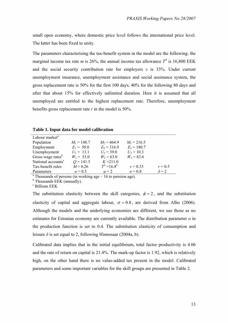
Table 1. Input data for model calibration

Labour marketa Population M1 = 148.7 M2 = 464.9 M3 = 216.5 Employment E1 = 50.0 E2 = 316.9 E3 = 180.7 Unemployment U1 = 13.1 U2 = 39.0 U3 = 10.3 Gross wage ratesb W1 = 53.0 W2 = 63.0 W3 = 83.6 National accountsc Q = 141.5 K =211.0 Tax-benefit rules M = 0.26 TA =16.8b ν = 0.33 r = 0.5 Parameters α = 0.5 φ = 2 σ = 0.8 δ = 2 a Thousands of persons (in working age – 16 to pension age). b Thousands EEK (annually). c Billions EEK

The substitution elasticity between the skill categories, 2=φ , and the substitution

elasticity of capital and aggregate labour, 8.0=σ , are derived from Alho (2006).

Although the models and the underlying economies are different, we use those as no

estimates for Estonian economy are currently available. The distribution parameter α in

the production function is set to 0.4. The substitution elasticity of consumption and

leisure δ is set equal to 2, following Hinnosaar (2004a, b).

Calibrated data implies that in the initial equilibrium, total factor productivity is 4.06

and the rate of return on capital is 21.4%. The mark-up factor is 1.92, which is relatively

high, on the other hand there is no value-added tax present in the model. Calibrated

parameters and some important variables for the skill groups are presented in Table 2.


14

Table 2. Calibrated parameters and variables by the skill types

Low-skilled Skilled High-

skilled Parameters The relative efficiency of a skill group, ie 1.00 8.96 8.99 The bargaining power of employers, iβ 0.88 0.49 0.56

The distribution parameter in the utility function, δ1id 0.15 0.27 0.34

The share of a skill group in public consumption, gi 0.18 0.56 0.26 Variables The share of a skill group in capital income 0.07 0.53 0.40

Average income tax rate on labour earnings, Lit 17.8% 19.1% 20.8%

Average income tax rate on unemployment benefits, Bit 9.5% 12.1% 15.6%

There is only a marginal difference between the relative efficiency of skilled and high-

skilled labour. The group of skilled has even stronger bargaining power compared to the

high-skilled. Each skill group’s share in public consumption is assumed to be

proportional to the number of respective households and therefore being exogenous.

The share in capital income is proportional to the aggregate wage earnings. Finally, the

values of the distribution parameter in the utility function reflect that those with higher

skills attribute a larger weight to consumption. This is due to higher unemployment

among lower skill groups, which in this framework translates (partly) into stronger

preferences for leisure.

4. Policy simulations

4.1. Description

There are four policy scenarios evaluated under all three wage systems, altogether up to

9 different simulations (some provide the same results). The following policy changes

are considered:

1) lowering the marginal income tax rate,

2) increasing the income tax allowance,

3) lowering employers’ social security contributions,

4) increasing the replacement rate.


15

All policy simulations are financed by an ex-ante reduction in the level of public

consumption by 0.5%. In terms of tax-benefit parameters this implies that (a) marginal

income tax rate is lowered from 0.26 to 0.222, (b) tax allowance is increased from

16,800 to 17,577 EEK per year, (c) employers’ social tax rate is decreased from 0.33 to

0.327, and (d) unemployment benefit replacement rate is increased from 0.5 to 0.541.

The two first policy shifts imitate actual income tax reforms in 2003 and 2005, which

will reduce the marginal income tax rate from 26% to 20% and double the annual tax

allowance from 12,000 to 24,000 EEK once fully implemented. However, here we do

not follow the actual policy changes in their exact magnitude as the different

simulations are balanced in fiscal terms in order to retain comparability. The latter two

scenarios are more hypothetical, carried out as the main alternatives. No simulation of

targeted policy changes in the form of e.g. a higher replacement rate for the low-skilled

have been undertaken. The results are presented in Table 3.


16

Table 3. Simulation results, percentage changes

(1) Lower mar-ginal income

tax rate

(2) Increased income tax allowance

(3) Lower employers’

social security contribution

(4) Increased

replacement rate

Policy scenarios

Target variables F, B M F, B M F M B F, M BProduction 0.0 0.9 0.0 -0.1 0.4 0.0 0.0 0.0 -2.7Private consumption 4.7 6.0 0.2 0.1 0.8 0.2 0.2 0.2 -3.5Public consumption -9.6 -7.1 -0.4 -0.6 0.8 -0.2 -0.3 -0.5 -8.4Social welfare 0.8 1.8 0.0 -0.1 0.5 0.1 0.0 0.0 -2.8 - low-skilled 0.2 0.3 0.0 0.0 0.3 0.0 0.0 0.1 -2.0 - skilled 0.4 1.3 0.0 0.0 0.5 0.1 0.0 0.1 -2.8 - high-skilled 1.3 2.5 0.0 -0.1 0.5 0.1 0.0 0.0 -2.9Labour supply 1.8 1.5 -0.2 -0.1 0.0 0.1 0.1 0.0 0.4 - low-skilled 5.7 4.3 -0.6 -0.5 0.0 0.1 0.2 0.0 1.3 - skilled 1.7 1.5 -0.1 -0.1 0.0 0.1 0.1 0.0 0.4 - high-skilled 0.7 0.7 0.0 0.0 0.0 0.0 0.0 0.0 0.2Employment 0.0 1.5 0.0 -0.1 0.6 0.1 0.0 0.0 -4.0 - low-skilled 0.0 4.3 0.0 -0.5 0.6 0.1 0.0 0.0 -4.0 - skilled 0.0 1.5 0.0 -0.1 0.6 0.1 0.0 0.0 -4.0 - high-skilled 0.0 0.7 0.0 0.0 0.6 0.0 0.0 0.0 -4.0Unemployment 17.5 2.0 -1.5 -0.2 -5.4 0.1 0.7 0.0 39.0 - low-skilled 27.6 4.3 -3.0 -0.5 -2.4 0.1 0.9 0.0 21.2 - skilled 15.1 1.5 -1.1 -0.1 -5.0 0.1 0.6 0.0 36.0 - high-skilled 13.7 0.7 -0.8 0.0 -10.9 0.0 0.6 0.0 73.2Gross wage rate - low-skilled -1.9 0.2 0.2 0.3 1.6 - skilled -0.6 0.0 0.2 0.3 1.6 - high-skilled

fixed -0.2

fixed0.0

fixed0.2 0.3

fixed 1.6

Unemployment ratea 1.6 -0.1 -0.6 0.1 0.0 3.9 - low-skilled 4.3 -0.5 -0.5 0.2 0.0 4.1 - skilled 1.4 -0.1 -0.6 0.1 0.0 3.9 - high-skilled 0.7

fixed

0.0

fixed

-0.6

fixed

0.0 0.0 3.9Note: F – fixed wages, M – market determined wages, B – wage bargaining. a Absolute changes in percentage points.

4.2. Lowering the marginal income tax rate

We can indeed observe increased private consumption with a lower marginal income

tax rate. On the other hand, tax revenues decline and therefore public consumption is

smaller. The overall impact on welfare depends on the social welfare function used. In

this case private and public consumption share the same distribution parameter and


17

social welfare also increases. Across the skill groups, more skilled persons gain more as

they have higher preference for their consumption (see the comments in Section 3).

In case of fixed (gross) wages only consumer wages decrease, producer wages do not

react and therefore production and labour demand will not be affected. Higher consumer

wages increase the labour supply. But employment is determined by the firms and

constant (as the producer wages are fixed), and the increased labour supply translates

one-to-one into higher unemployment.

Market determined wages are more flexible and the gross wage rate must decrease for

the unemployment rates to be unchanged. Therefore, the gains from reduced labour

taxes are shared between employers and employees. As producer wages decrease, more

labour is demanded and higher employment levels are attained. In the new equilibrium,

unemployment levels are only slightly higher and unemployment ratios are the same.

Yet, production also increases and therefore private consumption and social welfare

increase more than under fixed wages.

The wage bargaining case has the same outcome as fixed wages because the bargained

wages do not depend on the marginal tax rate. The lower marginal tax rate only

increases the labour supply, which has no (direct) effect on employment.

4.3. Increasing the income tax allowance

A larger income tax allowance also increases households’ disposable income. However,

the effect on the labour supply is exactly the opposite now. Under fixed wages this

transforms into lower unemployment as production and employment are not affected.

Private consumption increases a little, but the overall effect on social welfare is only

marginal. In case of market determined wages the decrease in labour supply is smaller.

This in turn requires a decline in employment and a lower gross wage rate. Production

also decreases and the overall effect on social welfare remains negative. Wage

bargaining yields again the same results as fixed wages.

4.4. Lowering employers’ social security contributions

Reducing the labour tax burden by lowering employers’ social security contributions

has a direct effect on labour demand and employment, but not on labour supply. Lower


18

labour costs increase production and employment. Again, as there is no mechanism

linking labour demand and supply, the latter remains unchanged with fixed wages and

unemployment declining. Higher employment and production increase private and

public consumption, therefore rising social welfare as well.

Fixed unemployment rates are attained via higher consumer wages and increased labour

supply, which makes this policy scenario less favourable under market determined

wages. Production increases only marginally, private consumption increases less than

under fixed wages and public consumption even decreases. Overall, social welfare is

somewhat higher.

This time wage bargaining leads to a different result compared to fixed wages, in fact

being closer to the outcome of market determined wages. The initial decrease in

producer wages transforms to higher gross wage rates. In the new equilibrium, producer

wages, employment and production have returned to initial levels. Higher consumer

wages attract additional labour supply causing unemployment levels to rise. Overall,

there is a small increase in private consumption, a small decrease in public consumption

and only a marginal improvement in social welfare.

4.5. Increasing the replacement rate

The increased replacement rate combined with either fixed wages or market determined

wages only implies slightly higher private consumption and social welfare. The reason

is that neither firms nor households take into account the extent of unemployment

benefits in their optimising behaviour. It does not affect labour costs for the firms and

households supply labour without considering the outside option. Unemployed

households are exogenously decided and therefore they do not take into account

unemployment benefits when choosing optimal labour to supply.

Under wage bargaining, higher unemployment benefits directly increase gross wage

rates, which in turn increases labour supply. Higher labour costs lower firms’ demand

for labour and therefore the employment level. As replacement rate is uniform across

the skill groups, the percentage changes in the gross wage rates and employment are

also the same. All this results in significantly higher unemployment, decreased

production, lower private and public consumption and lower social welfare.


19

5. Conclusions

The policy simulations considered show that alternative ways to “stimulate” the labour

market can lead to very different outcomes, e.g. on labour supply and unemployment.

An improvement in terms of households’ disposable income might even turn out to be

welfare reducing in the new equilibrium. The effects of policy changes also vary under

different wage formation schemes – lowering the marginal income tax rate is for

example most effective in enhancing private consumption and social welfare under

market determined wages while a reduction in the social tax rate works most

successfully under fixed wages. A combination of lowering marginal income tax rate

and increasing tax allowance, basically the recent tax reform, has a potential to increase

production and social welfare without increasing unemployment rates under market

determined wages.

Overall, the results are often similar to Hinnosaar (2004b) and Alho (2006) on which

our model is based. In comparison with the latter, the main differences occur where our

simulations yield identical results under various wage systems, highlighting some limits

of our model. However, assuming that different wage formations are relevant for

Estonian and Finnish economies (market determined wages and bargained wages,

respectively), we can stress the need for different labour market and tax-benefit policies

in different EU member states. Comparing the policy scenarios for Estonia under

market determined wages and wage bargaining implies that market determined wages

outperform bargained wages, the latter representing more EU-like wage formation.

Although no policy scenarios targeted at specific skill groups were carried out, some

implications could be still noted. The labour supply of low-skilled is most effectively

increased by lowering the marginal income tax rate, valid under every wage scheme.

Combining this in turn with strategies improving employment in general, e.g. lowering

employers’ social security contributions, could potentially improve the labour market

position of those with lower skills.


20

References

Alho, K. (2006). Labour market institutions and the effectiveness of tax and benefit

policies in enhancing employment: a general equilibrium analysis. ETLA Discussion

paper, No 1008.

Bovenberg, L.; Graafland, J.; Mooij, R. de (2000). Tax reform and the Dutch labor

market: an applied general equilibrium approach, Journal of Public Economics, No 78,

pp. 193-214.

Calmfors, L; Driffill, J. (1988). Bargaining Structure and Macroeconomic Performance,

Economic Policy, 6, April, pp. 13-61.

Carone, G.; Salomäki, A. (2001). Reforms in Tax-Benefit Systems in Order to Increase

Employment Incentives in the EU, ECFIN, Economic Paper, No. 160.

European Industrial Relations Observatory, Changes in national collective bargaining

systems since 1990. [http://www.eiro.eurofound.eu.int/2005/03/study/index.html]. Last

accessed: Nov 11, 2005.

Hinnosaar, M. (2004a). Estonian Labor Market Institutions within a General

Equilibrium Framework, Eesti Pank, Working Paper, No 5.

Hinnosaar, M. (2004b). The Impact of Benefit and Tax Reforms on Estonian Labor

Market in a General Equilibrium Framework, University of Tartu, Working Paper, No

31.

Labour Force Survey database. Statistical Office of Estonia, 2004.

Statistical Office of Estonia, Statistical Database. [http://www.stat.ee]. Last accessed:

Feb 6, 2006.


21

Appendix 1. A comparison of CGE models

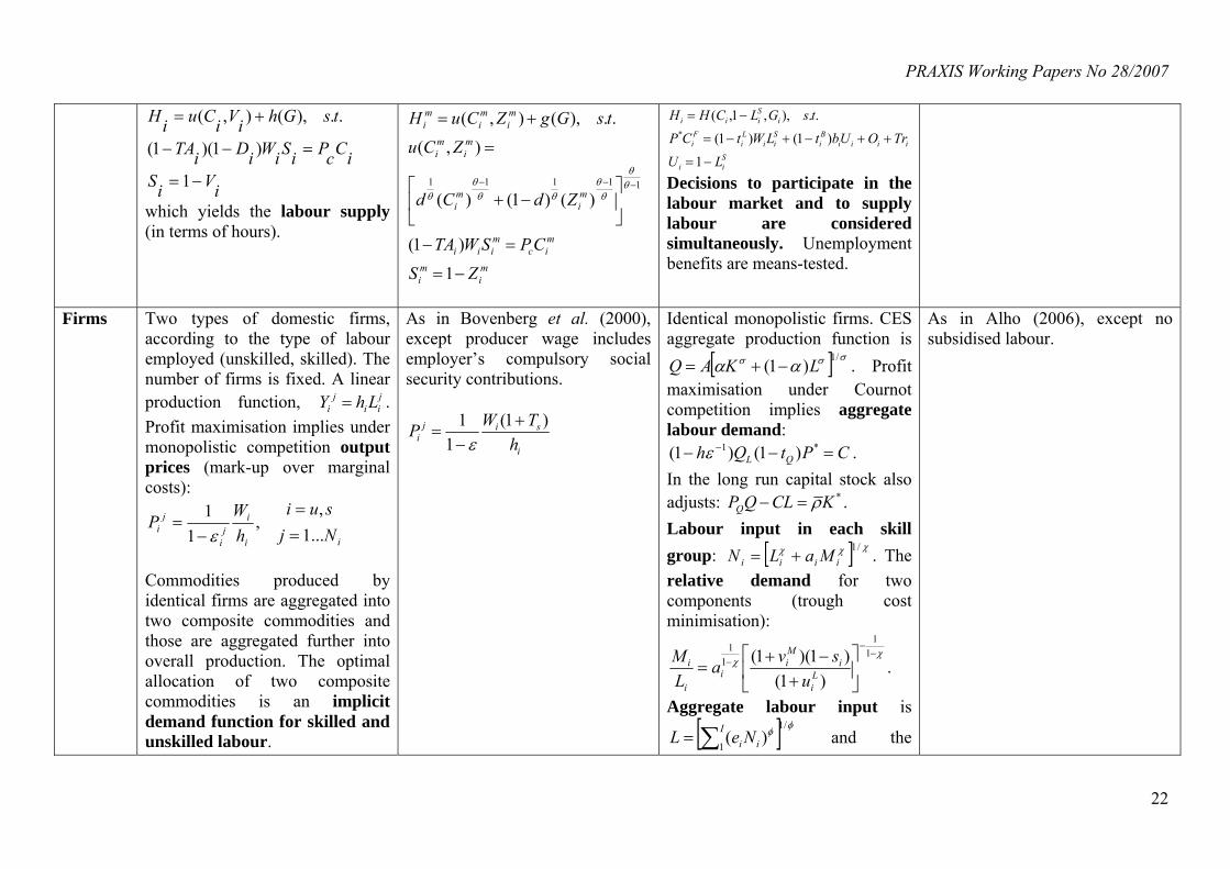
Model Bovenberg et al. (2000) Tax reform and the Dutch labor market: an applied general equilibrium approach, Journal of Public Economics, No 78, 2000, pp. 193-214.

Hinnosaar, M. (2004) a) Estonian Labor Market Institutions within a General Equilibrium Framework, Eesti Pank, No 5, 2004. b) The Impact of Benefit and Tax Reforms on Estonian Labor Market in a General Equilibrium Framework, University of Tartu, Working Paper, No 31, 2004.

Alho, K. (2006) Labour market institutions and the effectiveness of tax and benefit policies in enhancing employment: a general equilibrium analysis. ETLA Discussion paper, No 1008.

The current paper A Comparative General Equilibrium Analysis of the Estonian Labour Market. PRAXIS, Working Paper.

Back-ground

A simplification of MIMIC (a larger applied general equilibrium model for the Dutch economy).

Based largely on Bovenberg et al. (2000), without informal labour market, job matching and hiring costs. The wage formation for high-skilled workers is based on the efficiency wage concept.

Some similar elements with Bovenberg et al. (2000) (job matching and hiring costs). Additional input in production – capital.

Based on Hinnosaar (2004a, b) and Alho (2006).

House-holds

Three types of households: capitalists, unskilled and skilled households. Capitalists do not supply labour and receive all profit income. Participation decisions are exogenous, households choose the number of working hours. Households of each skill type maximise utility, subject to a budget and a time constraint (public consumption additively separable).

As in Bovenberg et al. (2000), except no hiring costs and tax progressivity due to tax allowance, not tax credit.

Three types of skill groups (low-skilled, skilled and high-skilled), each divided further as employed on market-based terms, employed on subsidised terms, unemployed and those outside the labour force. Individuals maximise utility subject to a budget and a time constraint:

As in Hinnosaar (2004a, b). Three skill groups instead of two. Workers receive distributed corporate profits, although it is not considered in labour supply (not anticipated).


22

iViSiCcPiSiWiDiTA

tsGhiViCuiH

−=

=−−

+=

1

)1)(1(

..),(),(

which yields the labour supply (in terms of hours).

mi

mi

mic

miii

mi

mi

mi

mi

mi

mi

mi

ZS

CPSWTA

ZdCd

ZCu

tsGgZCuH

−=

=−

⎥⎦

⎤⎢⎣

⎡−+

=

+=

−−−

1

)1(

)()1()(

),(

..),(),(

11111 θθ

θθ

θθθ

θ

Sii

iiiiBi

Sii

Li

Fi

iSiii

LU

TrOUbtLWtCP

tsGLCHH

−=

++−+−=

−=

1

)1()1(

..),,1,(*

Decisions to participate in the labour market and to supply labour are considered simultaneously. Unemployment benefits are means-tested.

Firms Two types of domestic firms, according to the type of labour employed (unskilled, skilled). The number of firms is fixed. A linear production function, j

iij

i LhY = . Profit maximisation implies under monopolistic competition output prices (mark-up over marginal costs):

ii

ij

i

ji Nj

suihW

P...1,

,1

1==

−=

ε

Commodities produced by identical firms are aggregated into two composite commodities and those are aggregated further into overall production. The optimal allocation of two composite commodities is an implicit demand function for skilled and unskilled labour.

As in Bovenberg et al. (2000), except producer wage includes employer’s compulsory social security contributions.

i

siji h

TWP )1(1

1 +−

=ε

Identical monopolistic firms. CES aggregate production function is

[ ] σσσ αα/1)1( LKAQ −+= . Profit

maximisation under Cournot competition implies aggregate labour demand:

CPtQh QL =−− − *1 )1()1( ε . In the long run capital stock also adjusts: *KCLQPQ ρ=− . Labour input in each skill group: [ ] χχχ /1

iiii MaLN += . The relative demand for two components (trough cost minimisation):

χχ

−−

−⎥⎦

⎤⎢⎣

⎡+

−+=

11

11

)1()1)(1(

Li

iMi

ii

i

usva

LM .

Aggregate labour input is

[ ] φφ /1

1)(∑=

Iii NeL and the

As in Alho (2006), except no subsidised labour.


23

relative demand for each skill group is

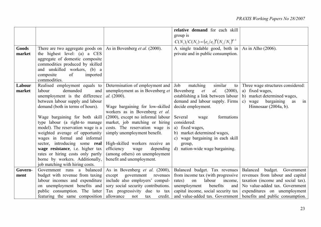
( ) ( ) 1111)()( −= φφ NNeeNCNC iii

Goods market

There are two aggregate goods on the highest level: (a) a CES aggregate of domestic composite commodities produced by skilled and unskilled workers, (b) a composite of imported commodities.

As in Bovenberg et al. (2000). A single tradable good, both in private and in public consumption.

As in Alho (2006).

Labour market

Realised employment equals to labour demanded and unemployment is the difference between labour supply and labour demand (both in terms of hours). Wage bargaining for both skill type labour (a right-to manage model). The reservation wage is a weighted average of opportunity wages in formal and informal sector, introducing some real wage resistance, i.e. higher tax rates or hiring costs only partly borne by workers. Additionally, job matching with hiring costs.

Determination of employment and unemployment as in Bovenberg et al. (2000). Wage bargaining for low-skilled workers as in Bovenberg et al. (2000), except no informal labour market, job matching or hiring costs. The reservation wage is simply unemployment benefit. High-skilled workers receive an efficiency wage depending (among others) on unemployment benefit and unemployment.

Job matching similar to Bovenberg et al. (2000), establishing a link between labour demand and labour supply. Firms decide employment. Several wage formations considered: a) fixed wages, b) market determined wages, c) wage bargaining in each skill

group, d) nation-wide wage bargaining.

Three wage structures considered: a) fixed wages, b) market determined wages, c) wage bargaining as in

Hinnosaar (2004a, b).

Govern-ment

Government runs a balanced budget with revenue from taxing labour incomes and expenditure on unemployment benefits and public consumption. The latter featuring the same composition

As in Bovenberg et al. (2000), except government revenues include also employers’ compul-sory social security contributions. Tax progressivity due to tax allowance not tax credit.

Balanced budget. Tax revenues from income tax (with progressive rates) on labour income, unemployment benefits and capital income, social security tax and value-added tax. Government

Balanced budget. Government revenues from labour and capital taxation (income and social tax). No value-added tax. Government expenditures on unemployment benefits and public consumption.


24

and price index as private consumption.

Unemployment benefits combine subsistence benefit and universal unemployment benefit.

expenditures on unemployment benefits, wage subsidies and public consumption.

Unemployment benefit is a fixed proportion of gross wage.

Foreign sector

The allocation of foreign consumption over domestic and foreign goods depends on the terms of trade. The market of domestic goods is in equilibrium.

As in Bovenberg et al. (2000). Demand for domestic products depends on the international price level (given for a small open economy). Otherwise not explicitly modelled.

As in Alho (2006).

Data and the key para-meters

Dutch economy in 2018. Substitution elasticity between skill groups 1.5, substitution elasticity of consumption and leisure 4, uncompensated wage elasticity 0.15, income elasticity -0.05, export elasticity -2.

Estonian economy in 2001, import structure from 1997. Substitution elasticity between skill groups 0.5, substitution elasticity of consumption and leisure 2, Armington elasticity and transformation elasticity 2.

Finnish economy in 2002. Substitution elasticity between skill groups 2, substitution elasticity of capital and aggregate labour 0.8, distribution parameter in production function 0.4, substitution elasticity of consumption and leisure 0.5.

Estonian economy in 2004. Substitution elasticity between skill groups 2, substitution elasticity of capital and aggregate labour 0.8, distribution parameter in production function 0.5, substitution elasticity of consumption and leisure 2.

Simula-tions

1) Lowering marginal tax rate (benefits indexed to consumer wages)

2) Higher tax credit for all households (benefits indexed to consumer wages)

3) Higher tax credit for all households (benefits indexed to producer wages)

4) Higher tax credit for unskilled workers (benefits indexed to producer wages)

5) Higher tax credit for all workers, higher marginal tax rate, skilled workers break

Hinnosaar 2004a: 1) Higher union bargaining

power, i.e. higher wage for low-skilled workers

2) Higher unemployment benefits replacement rate for all workers

3) Higher unemployment benefits replacement rate for high-skilled workers

4) Increasing tax allowance for all workers

5) Increasing tax allowance for low-skilled workers

1) Lowering income tax rate a) average (and marginal) b) marginal (only)

2) Lowering employers’ social security contributions for

a) all skill groups b) low-skilled workers

3) Higher wage subsidy rates 4) Lower unemployment benefit

replacement rates 5) Reducing unemployment in a

fully flexible labour market Financed by ex ante decrease in public consumption by 0.5% in 1)

1) Lowering marginal income tax rate

2) Increasing tax allowance 3) Lowering employers’ social

security contributions 4) Increasing replacement rate. Financed ex ante decrease in public consumption by 0.5%.


25

even ex ante (benefits indexed to producer wages)

Financed by ex ante reduction in public consumption (0.5% GDP).

Hinnosaar (2004b), reforms financed by ex ante decrease in public consumption by 0.5%: 1) Lowering marginal tax rate 2)-5) As in Hinnosaar (2004a).

and 2), 0.07% in 3), 0.18% in 4).

Results Paper demonstrates various trade-offs facing tax reforms. Simulations highlight in-work benefits as an effective instrument against unemployment.

Reducing tax burden via targeted increase in tax allowance has the most favourable impact on the labour market.

Simulations show that wage formation is an important factor for employment enhancing policies. In some cases the expansionary effects are even the largest under wage bargaining.

Simulations show that market determined wages outperform bargained wages. The labour market position of the low-skilled could be improved most effectively by lowering the marginal tax rate and employers’ social security contributions.


26

Appendix 2. Labour supply

Individuals maximise the CES sub-utility function

( ) ( ) ( ) 11111

1),(−−−

⎥⎦

⎤⎢⎣

⎡−+=

δδ

δδ

δδδ

δ jii

jii

ji

ji VdCdVCh (20)

subject to the time constraint ji

ji VS −=1 and the budget constraint

ji

jii

Li PCSWt =− )1( (21)

Substituting constraints into the utility function:

( ) ( ) ( ) 11111

1

11)1(max−−−

−⎥⎦

⎤⎢⎣

⎡−−+−=

δδ

δδ

δδδ

δ jii

jii

Lii

SSdPSWtdh

ji

(22)

FOC, note that Ajii

jii

Li mTSWmSWt +−=− )1()1( :

( )( ) ( ) ( )

( )( ) ( ) ( ) ( ) 0)1(111)1(

11)1(

111

11

1

11

1111

1

=⎥⎦

⎤⎢⎣

⎡−−−+−+−

⋅⎥⎦

⎤⎢⎣

⎡−−++−

−−−−

−−−−

δδδδ

δδδ

δδδ

δ

jiii

Ajiii

jii

Ajiii

SdPWmPmTSWmd

SdPmTSWmd (23)

Solving for labour supply3:

( ) ( )( ) ( )⇒−=−+−− −−− j

iiAj

iii

i SPWmPmTSWmd

d11)1(

1 11 δ (24)

( )( )

( )( ) δ

δ

−−−

−−−

−−

−+

−−

−=

11

11

11

)1(1

11

1

PWmPd

dWm

PWmPd

dmT

Si

i

ii

ii

iA

ji (25)

Total labour supply is

( )( )

( ) δ

µµµ −

⎟⎠⎞

⎜⎝⎛ −−

=−+−

==P

WmPd

dWm

mTMSMS i

i

i

i

Aij

iii111,

111 (26)

3 Note that this is different compared to Bovenberg et al. (2000) and Hinnosaar (2004a, b). There a household’s labour supply was also expressed in terms of average tax rate, which in return depends on household’s labour supply.


27

Appendix 3. Labour cost

The aggregate labour cost minimisation problem:

( )∑=i iiN

NNCCi

min (27)

subject to

( )[ ] LNei ii =∑ φφ

1

(28)

The Lagrangian function is:

( ) ( )[ ]⎭⎬⎫

⎩⎨⎧

−−= ∑∑ LNeNNCLi iii iiNi

φφλ1

ˆmin (29)

FOC:

( ) ( )[ ] ( ) 0ˆ 1

)1(

=−=∂∂ −

−

∑ iiii iiii

eNeNeNCNL φφ

φφλ (30)

Divide by ijNL j ≠∂∂ ,ˆ :

( )( )

φ

⎟⎟⎠

⎞⎜⎜⎝

⎛=

jj

ii

jj

ii

NeNe

NNCNNC (31)

Sum over ( )jini ≠= ...1 and add one to both side for ji = :

( )( )

( )( )φ

φ

jj

i ii

jj

i ii

NeNe

NNCNNC ∑∑ = (32)

Substitute (27) and (28) into (32), solve for Nj:

( )φφ

φ

φ

−−

⎟⎟⎠

⎞⎜⎜⎝

⎛⎟⎠⎞

⎜⎝⎛=

11

11

j

jj NC

eLCN (33)

Multiply by ( )jNC and sum over nj ...1=

( ) ( )∑∑−−

⎟⎟⎠

⎞⎜⎜⎝

⎛⎟⎠⎞

⎜⎝⎛==

jj

jj jj NC

eLCNNCC

φφ

φ

φ

111

(34)

Solve for aggregate labour cost, C:

( ) φφ

φφ

−−

−−

⎟⎟⎟

⎠

⎞

⎜⎜⎜

⎝

⎛

⎟⎟⎠

⎞⎜⎜⎝

⎛= ∑

1

1

jj

j

eNC

LC (35)


28

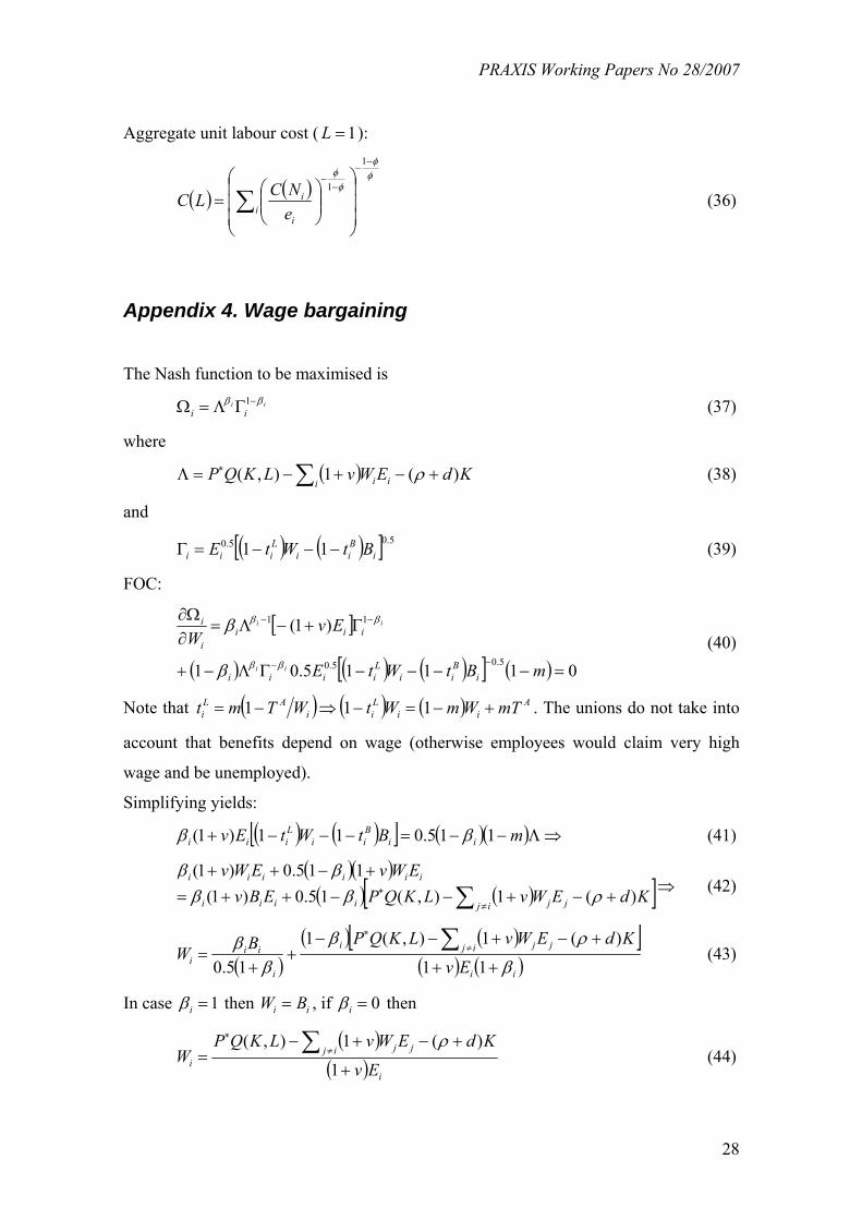
Aggregate unit labour cost ( 1=L ):

( ) ( )φφ

φφ

−−

−−

⎟⎟⎟

⎠

⎞

⎜⎜⎜

⎝

⎛

⎟⎟⎠

⎞⎜⎜⎝

⎛= ∑

1

1

ii

i

eNCLC (36)

Appendix 4. Wage bargaining

The Nash function to be maximised is ii

iiββ −ΓΛ=Ω 1 (37)

where

( ) KdEWvLKQPi ii )(1),( +−+−=Λ ∑∗ ρ (38)

and

( ) ( )[ ] 5.05.0 11 iBii

Liii BtWtE −−−=Γ (39)

FOC:

[ ]

( ) ( ) ( )[ ] ( ) 01115.01

)1(

5.05.0

11

=−−−−ΓΛ−+

Γ+−Λ=∂Ω∂

−−

−−

mBtWtE

EvW

iBii

Liiii

iiii

i

ii

ii

ββ

ββ

β

β (40)

Note that ( ) ( ) ( ) Aii

Lii

ALi mTWmWtWTmt +−=−⇒−= 111 . The unions do not take into

account that benefits depend on wage (otherwise employees would claim very high

wage and be unemployed).

Simplifying yields:

( ) ( )[ ] ( )( ) ⇒Λ−−=−−−+ mBtWtEv iiBii

Liii 115.011)1( ββ (41)

( )( )( ) ( )[ ]⇒+−+−−++=

+−++

∑ ≠∗ KdEWvLKQPEBv

EWvEWv

ij jjiiii

iiiiii

)(1),(15.0)1(115.0)1(

ρββββ

(42)

( )( ) ( )[ ]

( ) ( )ii

ij jji

i

iii Ev

KdEWvLKQPBWβ

ρβ

ββ

++

+−+−−+

+=

∑ ≠∗

11

)(1),(1

15.0 (43)

In case 1=iβ then ii BW = , if 0=iβ then

( )( ) i

ij jji Ev

KdEWvLKQPW

+

+−+−=

∑ ≠∗

1

)(1),( ρ (44)

Documents

A Comparative General Equilibrium Analysis of the …€¦ · 28 A Comparative General Equilibrium Analysis of the Estonian Labour Market Alari Paulus Andres Võrk Kari E. O. Alho