A Comparative Analysis of Weaving Areas in HCM, TRANSIMS, CORSIM, VISSIM and INTEGRATION

Nanditha Koppula Thesis submitted to the Faculty of the Virginia Polytechnic Institute and State University

in partial fulfillment of the requirements for the degree of

Master of Science

In

Civil and Environmental engineering

Antoine Hobeika

Antonio A.Trani

Sam Tignor

April 2002

Blacksburg, Virginia.

Keywords : Weaving sections, HCM, TRANSIMS, CORSIM, VISSIM, INTEGRATION

A Comparative Analysis of the Weaving Areas in HCM, TRANSIMS, CORSIM, VISSIM and INTEGRATION

Nanditha Koppula

Abstract

Traffic simulation is a powerful tool that provides transportation engineers with the

ability to test the feasibility and performance of a system before it is implemented and

also helps in optimizing the proposed system. Over the past twenty years significant

amount of work has been conducted on improving the quality and accuracy of

transportation simulation models. Much of this work has been concentrated on

microscopic simulation models because they provide traffic engineers greater opportunity

to examine the inherently complex, stochastic, and dynamic nature of transportation

systems when compared to traditional macroscopic models. In order to test the

performance of some of the simulation models, a study is conducted on freeway weaving

sections, which are considered to be one of the most complex regions to be modeled and

analyzed. The intent of the research is to evaluate TRANSIMS, CORSIM, VISSIM and

INTEGRATION and compare them with Highway Capacity Manual, which adopts a

traditional methodology for carrying out the operational analysis of a highway system.

The statistics collected for the simulation runs include weaving speeds, non-weaving

speeds and density of the weaving section.

ii

Acknowledgements I would like to express my sincere appreciation to Dr. Antoine Hobeika for his continued

support and guidance throughout the development of the thesis. I also express my

appreciation to the members of my committee, Dr. Trani and Dr. Tignor. I would like to

take this opportunity to thank all the members of the Faculty in the Civil Engineering

Department.

I would like to dedicate this thesis to my parents, Laxma Reddy and Jana Koppula,

brother Praneeth Reddy Koppula, sister Haritha Minkuri and brother in law Venu Gopal

Reddy Minkuri for their encouragement and continued support throughout my studies.

I would like to express my gratitude to Mr. Tirumal Rao, Dr. Baik and Srinivas J. for

their timely advice and support. I would like to sincerely thank all my friends Senanu A.,

Srikanth G., Sulakshana P., Priya N., Pramod M., Sudheer D., Bindu V., Sunita K.,

Poonam K. who have encouraged me in all aspects of life and helping me build a career.

iii

Table of Contents

ABSTRACT ....................................................................................................................... II

ACKNOWLEDGEMENTS..............................................................................................III

TABLE OF CONTENTS................................................................................................. IV

LIST OF FIGURES........................................................................................................VII

LIST OF TABLES ........................................................................................................VIII

CHAPTER 1 : INTRODUCTION..................................................................................... 1 1.1 BACKGROUND...................................................................................................... 1 1.2 PROBLEM DEFINITION.......................................................................................... 2 1.3 THESIS OBJECTIVE ............................................................................................... 2 1.4 ORGANIZATION OF THESIS ................................................................................... 3

CHAPTER 2 : LITERATURE REVIEW.......................................................................... 4 2.1 INTRODUCTION .................................................................................................... 4 2.2 PURPOSE OF THIS CHAPTER ................................................................................... 6 2.3 TRAFFIC SIMULATION PACKAGES ............................................................................ 6

2.3.1 TRANSIMS........................................................................................... 6 2.3.2 CORSIM................................................................................................ 7 2.3.3 VISSIM.................................................................................................. 7 2.3.4 INTEGRATION .................................................................................... 8

2.4 SIMULATION ........................................................................................................ 8 2.5 VEHICULAR TRAFFIC THEORY .......................................................................... 10

2.5.1 Traffic Flow Theory - Macroscopic Model......................................... 10 2.5.1.1 Greenshields Model ............................................................................... 11 2.5.1.2 Greenberg Model ................................................................................... 12 2.5.1.3 Underwood’s Model .............................................................................. 12 2.5.1.4 Drew’s Model ........................................................................................ 13

2.5.2 Car Following Theory - Microscopic Models .................................... 13 2.5.2.1 Pipes' theory of car-following................................................................ 15 2.5.2.2 Forbes' theory of car-following.............................................................. 16 2.5.2.3 GM-model of car-following................................................................... 18

2.5.3 Particle Hopping Theory – Mesoscopic Model................................... 20 2.5.3.1 The Stochastic Traffic Cellular Automaton (STCA) ............................. 21 2.5.3.2 The Deterministic Limit of the STCA (CA-184)................................... 23 2.5.3.3 The Asymmetric Stochastic Exclusion Process (ASEP) ....................... 23

2.6 SPECIFIC CHARACTERISTICS OF THE SIMULATION PACKAGES............................ 24 2.6.1 TRANSIMS ..................................................................................... 24

2.6.1.1 Vehicle Movement In The Same Lane .................................................. 25 2.6.1.2 Lane Changing logic .............................................................................. 30 2.6.1.3 Vehicle Movements at Intersections...................................................... 37

2.6.2 CORSIM .......................................................................................... 42

iv

2.6.2.1 FRESIM Model...................................................................................... 42 2.6.2.2 NETSIM Model ..................................................................................... 49

2.6.3 VISSIM............................................................................................ 52 2.6.3.1 Car Following Logic .............................................................................. 53 2.6.3.2 Lane Changing Logic............................................................................. 56

2.6.4 INTEGRATION .................................................................................. 57 2.6.4.1 Vehicle Movement Logic ...................................................................... 57 2.6.4.2 Car Following Logic .............................................................................. 58 2.6.4.3 Lane Changing Logic............................................................................. 59 2.6.4.4 Vehicle Movements at Intersections...................................................... 61

2.7 COMPARISON AND CONTRAST BETWEEN TRANSIMS, CORSIM VISSIM AND INTEGRATION ........................................................................................................... 61 2.8 DESCRIPTION OF THE WEAVING SECTIONS ........................................................ 64

2.8.1 HCM Methodology........................................................................ 69 2.9 PAST RESEARCH RELATED TO FREEWAY WEAVING ANALYSIS ......................... 75

CHAPTER 3: DESCRIPTION OF THE RAMP-WEAVE MODEL............................. 78

3.1 INTRODUCTION .................................................................................................. 78 3.2 ASSUMPTIONS.................................................................................................... 78 3.3 THE MODELING CONCEPTS................................................................................ 80

3.3.1 HCM ................................................................................................ 80 3.3.2 TRANSIMS...................................................................................... 80 3.3.3 CORSIM........................................................................................... 81 3.3.4 VISSIM............................................................................................. 81 3.3.5 INTEGRATION ............................................................................... 82

3.3 DESCRIPTION OF CONFIGURATIONS ................................................................... 82

CHAPTER 4: COMPARING HCM, TRANSIMS, CORSIM, VISSIM AND INTEGRATION RESULTS ............................................................................................ 91

4.1 CALIBRATION PARAMETERS FOR THE MODELS.................................................. 91 4.1.1 TRANSIMS ..................................................................................... 91 4.1.2 CORSIM.......................................................................................... 94 4.1.3 VISSIM............................................................................................ 96 4.1.4 INTEGRATION .............................................................................. 96

4.2 CALIBRATION TESTS AND SENSITIVITY ANALYSIS........................................... 100 4.3 FINAL RESULTS OF ANALYSIS IN HCM, CORSIM, VISSIM, INTEGRATION AND TRANSIMS ................................................................................................................ 107

CHAPTER 5 : CONCLUSIONS AND RECOMMENDATIONS................................ 119 5.1 CONCLUSIONS...................................................................................................... 119 5.2 RECOMMENDATIONS........................................................................................... 120

BIBLIOGRAPHY........................................................................................................... 122

APPENDIX A................................................................................................................. 125

APPENDIX B................................................................................................................. 154

v

APPENDIX C................................................................................................................. 164

APPENDIX D ................................................................................................................ 210

vi

List of Figures Figure 1: A Car Following Theory ................................................................................... 15 Figure 2: In-Lane Movement Of Car1 Based On Gaps At T=t ........................................ 27 Figure 3: Position And Speed Of Car 1 Based On Gaps At T=t+1 ................................. 27 Figure 4: Flowchart For General Movement Of Vehicles In The Same Lane ................ 29 Figure 5: Left Lane Change Considerations For Car 1 At T=t ....................................... 31 Figure 6: Right Lane Change For Car1 ........................................................................... 31 Figure 7: Example For Lane Change Based On Plan Following ................................... 34 Figure 8: A Flowchart Representing the Lane Change Procedures ................................ 36 Figure 9: Vehicle Movement At An Unsignalized Intersection. ....................................... 40 Figure 10: Car Following................................................................................................. 44 Figure 11: Lane Change Parameters ............................................................................... 45 Figure 12: Gap Acceptance .............................................................................................. 51 Figure 13: Car Following Logic....................................................................................... 55 Figure 14 a & b: Type A Weaving Sections (Source HCM) ............................................. 65 Figure 15: Type B Weaving Sections (Source HCM) ....................................................... 67 Figure 16: Type C Weaving Sections (Source HCM) ....................................................... 68 Figure17: Methodology Adopted in the Research ............................................................ 79 Figure 18: Analysis of Ramp-Weave section .................................................................... 83 Figure 19: Analysis of major weaving segment................................................................ 83 Figure 20: Analysis of Alternative Major Weaving Segments.......................................... 84 Figure 21: Node Representation of Type A for TRANSIMS ............................................. 85 Figure 22: Node Representation of Type A for CORSIM and INTEGRATION ............... 86 Figure 23: Node Representation of Type B for TRANSIMS ............................................. 87 Figure 24: Node Representation of Type B for CORSIM and INTEGRATION ............... 88 Figure 25: Node Representation of Type C for TRANSIMS ............................................. 89 Figure 26: Node Representation of Type C for CORSIM and INTEGRATION ............... 90 Figure 27: Time-Space Diagrams for a typical vehicle in TRANSIMS ............................ 98 Figure 28: Time-Space Diagrams for a typical vehicle in CORSIM................................ 98 Figure 29: Time-Space Diagrams for a typical vehicle in VISSIM .................................. 99 Figure 30: Time-Space Diagrams for a typical vehicle in INTEGRATION ................... 100 Figure 31: Comparison of Velocities by Movement Type for different Test Cases in

TRANSIMS .............................................................................................................. 102 Figure 32: Comparison of Velocities for different Test Cases in TRANSIMS and HCM103 Figure 33: Comparison of Densities for different Test Cases in TRANSIMS and HCM.104 Figure 34: Comparison of Velocities for different Test Cases in CORSIM and HCM…106 Figure 35: Comparison of Velocities for different Test Cases in TRANSIMS and

HCM…………………………………………………………………………………………106 Figure 36: Comparison of Velocities for different Test Cases in CORSIM and HCM…107 Figure 37: Results for Type A Configuration ................................................................. 113 Figure 38: Results for Type B Configuration ................................................................. 115 Figure 39: Results for Type C Configuration ................................................................. 117

vii

List of Tables Table 1: Computation Of Weights For Lane Changes For Passing Slower Vehicles …..31 Table 2: Traffic Control States And Corresponding Actions …………………………...38 Table 3: Acceptable Gap Size …………………………………………………………...51 Table 4: Configuration Type versus Minimum Number of Required Lane Changes …...68 Table 5: Type of Configuration vs Constant Values …………………………………….71 Table 6: Criteria For Unconstrained versus Constrained Operation Of Weaving Areas 72 Table 7: LOS Criteria for Weaving Areas ………………………………………………73 Table 8: Sensitivity analysis using configuration keys ………………………………...101 Table 9: Comparison of Velocities by Movement Type for different Test Cases in TRANSIMS ……………………………………………………………………………..102 Table 10: Comparison of Velocities for different Test Cases in TRANSIMS and HCM .103 Table 11: Comparison of Densities for Test Cases in TRANSIMS and HCM …………104 Table 12: Default values used in CORSIM. …………………………………………...105 Table 13 : Compariosn of Velocities for different test cases in CORSIM and HCM..….106 Table 14 : Compariosn of Velocities for different test cases in CORSIM and HCM..….106 Table 15 : Compariosn of Velocities for different test cases in CORSIM and HCM..….107 Table 16: Comparison of Velocities and Density in HCM, TRANSIMS, CORSIM, VISSIM and INTEGRATION for Type A Configuration ……………………………….110 Table 17: Comparison of Velocities and Density in HCM, TRANSIMS, CORSIM, VISSIM and INTEGRATION forType B Configuration ………………………………………...111 Table 18: Comparison of Velocities and Density in HCM, TRANSIMS, CORSIM, VISSIM and INTEGRATION for Type C Configuration ……………………………….112

viii

Chapter 1 : Introduction

1.1 Background

Simulation is a valuable tool that is widely used in a variety of fields due to its ability to

provide realistic results. Simulation modeling has gained recognition as an effective

approach for quantifying traffic operations as transportation systems have become more

complex. Traffic simulation is a powerful tool that provides transportation engineers with

the ability to test the feasibility and performance of a system before it is implemented,

and also helps in optimizing the proposed system. Traffic simulation models are

established tools for assessing the network and freeway issues and are used for analyzing

traffic. Several different types of simulation packages are available, from detailed

microscopic models to macroscopic flow models, each with a particular role depending

upon the type of analysis desired. Some of the various simulation models that can be used

for traffic modeling and analysis are CORSIM (CORridor SIMulation), VISSIM,

INTEGRATION and TRANSIMS (TRansportation ANalysis and SIMulation System).

There is little information available to analysts applying these tools to simulate freeway

weaving sections, about the most appropriate models to choose. To address this need, a

detailed and technical comparison of the above mentioned simulation models is provided.

CORSIM, VISSIM and INTEGRATION adopt microscopic modeling approach. A

microscopic modeling approach is adopted where there is a need to obtain the system

entities and their interactions at a high level of detail. The microscopic approach

possessing the potential to be more accurate than its less detailed counterparts, involves a

lot of complexity in the logic of the core algorithms, as a large number of parameters

need to be calibrated. The core algorithm logic includes various factors like car following

logic, lane change behavior and vehicle movements at intersections, which are discussed

in detail later. Early car following theory of microscopic simulation models is based on

research first conducted at the General Motors Research Labs in the middle and late

1950’s.

1

In order to obtain a less computationally intensive and complex modeling approach,

unlike microscopic models, mesoscopic approach is used which generally represents

most entities at a high level of detail but describes their activities and interactions at a

much lower level of detail. TRANSIMS uses this approach. It uses particle hopping

theory, where vehicle movements take place by hopping from one cell to another. This

kind of approach is used where a large network has to be simulated as it adopts simple

rule based algorithms.

1.2 Problem Definition On freeways, weaving areas are the most complex regions to be modeled. Weaving

sections require intense lane changing maneuvers, as drivers must access lanes

appropriate to their desired exit point. It is important to model weaving behavior

accurately, as the overall performance of networks can be influenced by traffic behavior

at weave sections. There is little information available in literature regarding the

performance of different simulation models at freeway weave sections, and therefore, the

most appropriate model to use for analyzing these areas.

1.3 Thesis Objective

The objective of the thesis is to compare the core algorithm logics of the simulation

models, TRANSIMS, CORSIM, VISSIM and INTEGRATION. A comparative analysis

of weaving areas is then conducted using these models. The methodology adopted in

Highway Capacity Manual (HCM) is taken as the basis for the comparison of models.

This methodology evolved from a wide range of empirical research conducted since

1960’s. The different configurations of weaving areas, Type A, Type B and Type C are

considered for analysis. The statistics collected for the simulation runs include weaving

speeds, non-weaving speeds and density of the weaving section. The models are

calibrated by conducting a sensitivity analysis taking the HCM results as a base. The

simulation model giving best results with respect to HCM is identified.

2

1.4 Organization of Thesis

The thesis is organized as follows: Chapter 2 presents a literature review of previous

studies related to this research. It discusses the modeling of vehicular traffic using car

following theory and particle hopping theory. Specific characteristics of each simulation

model being considered in this research are described. The methodologies used by HCM

for analysis of freeway weaving sections are then discussed.

The different configurations of weaving sections are compared, analyzed and modeled in

Chapter 3. A discussion of the modeling strategies adopted to model these configurations

is then presented.

Chapter 4 presents a sensitivity analysis conducted for the models and then a comparison

of results. The conclusions and recommendations for future research are detailed in

chapter 5.

Appendix A shows the data used for analysis and validation. The data used for plotting

various graphs is shown in Appendix B.

3

Chapter 2 : Literature Review

2.1 Introduction

The main focus of this thesis is to carry out a comparative analysis of weaving sections of

configuration types A, B and C on freeways using TRANSIMS, CORSIM, VISSIM and

INTEGRATION. Hence, it is important to understand the treatment of vehicle

movements in weaving sections in the models.

A coarse simulation modeling approach, “Cellular Automata” is adopted by TRANSIMS

to keep up with the fast computational speed necessary to simulate a whole region. The

Cellular Automata approach divides every link on the network into a finite number of

cells. It incorporates particle-hopping theory where the vehicle movements take place by

hopping from one cell to another. Vehicles in the network follow simple rules that govern

their movements. At the core, the rules for a vehicle movement in the same lane could be

put simply as “Acceleration whenever possible, Deceleration only if necessary and

sometimes for no reason”. The decision by a vehicle to accelerate or decelerate depends

on its current speed and the gap between it and the immediate vehicle ahead in the same

lane. Lane change maneuver is considered by a vehicle based on either passing slower

vehicle or based on following its plan. The central idea of lane changing logic is the

availability of forward and backward gaps in the adjacent lanes. TRANSIMS does not

have a separate logic for weaving sections but incorporates algorithms based on ‘vehicle

movement logic in the same lane’ and ‘lane changing logic’.

CORSIM uses the Pitts car-following model, developed by University of Pittsburgh. The

basic concept of this model is vehicle movements take place considering the headway

between the follower car and the lead car. The model includes a comprehensive lane

changing logic representing different sides of lane changing process namely gap

evaluation, gap acceptance and the driver decision to perform a lane change. Gap

evaluation refers to the process of evaluating the lead gap and trailing gap sizes. Gap

acceptance refers to the process of determining whether the lead and trailing gaps are

4

acceptable to the lane changer and putative follower. In CORSIM there is no separate

treatment for weaving areas.

VISSIM uses a psychophysical car following model for longitudinal vehicle movement,

and a rule-based algorithm for lateral movements. The basic concept of this model is that

the driver of a faster moving vehicle starts to decelerate as he reaches his individual

perception threshold to a slower moving vehicle. Since he cannot exactly determine the

speed of that vehicle, his speed will fall below that vehicle’s speed until he starts to

slightly accelerate again after reaching another perception threshold. This results in an

iterative process of acceleration and deceleration. Lane changing behavior forms a part of

core algorithm logic, which considers acceptable gaps in neighboring lanes. VISSIM

simulates traffic flow by moving “driver- vehicle- units” through a network. As a

consequence, the driver behavior corresponds to the technical capabilities of the vehicle.

In VISSIM there is no separate logic for weaving movements but the behavior is

emergent from the car following and lane changing logic.

INTEGRATION uses a steady state car following model that combines Pipes and

Greenshields models into a single regime model, which is a four-parameter model. The

car-following model selects the desired speeds of vehicles by considering only the

attributes of other vehicles ahead of it in the same lane. It provides separate deceleration

and acceleration logic. Lane changing behavior that incorporates gap evaluation and gap

acceptance logic forms a part of core algorithm logic. Within INTEGRATION the impact

of a weaving section is a direct function of the interaction between the prevailing car-

following and lane-changing behavior but it has no separate weaving logic. The weaving

logic is sensitive to the type of weave that takes place, as different numbers of lane

changes are required per vehicle for different weave types. The model is also sensitive to

the length of the weave, as a longer weaving section permits the impact of the lane

changes to be spread out over a longer length of road segment. The weaving logic and

impacts are emergent features of the default model logic, and therefore do not require the

modeler to tag specific sections as being weaving sections. Therefore, any area in which a

large number of mandatory lane changes are necessary will automatically experience

5

weaving impacts. Furthermore, the magnitude of the capacity reduction will dynamically

depend upon the mix of weaving versus non-weaving flows. (Integration user’s guide)

2.2 Purpose of this chapter In this chapter, the literature behind the core algorithm logic for the simulation models is

discussed. As a part of core algorithm logic vehicle movements, car following logic and

lane changing logic in all the models is detailed. The various analytical models, which led

to the development of the current version of the simulation models, are discussed. The

specific characteristics of these models are brought out and a comparative analysis is

provided. Past and current research on these factors is also elaborated.

2.3 Traffic Simulation Packages

A brief description of the models that are used for the comparative analysis of freeway

weaving sections in this study is provided here.

2.3.1 TRANSIMS

TRANSIMS is a mesoscopic simulation model, which consists of mutually supporting

simulations, models, and databases that employ advanced computational and analytical

techniques to create an integrated regional transportation system analysis environment.

By applying advanced technologies and methods, it simulates the dynamic details that

contribute to the complexity inherent in transportation issues. The integrated results from

the detailed simulations help address environmental pollution, energy consumption,

traffic congestion, land use planning, traffic safety, intelligent vehicle efficiencies, and

the transportation infrastructure effect on quality of life, productivity, and economy.

TRANSIMS was developed by The Los Alamos National Laboratory (LANL). It is a part

of the Travel Model Improvement Program sponsored by the U.S. Department of

Transportation, the Environmental Protection Agency, and the Department of Energy.

TRANSIMS operates on Unix and Linux operating systems only. (TRANSIMS website).

6

2.3.2 CORSIM

CORSIM is a microscopic simulation model of the TRAF system designed for the

analysis and modeling of freeways, surface streets, corridors or networks and basic transit

operations. The model includes two predecessor models that operate on a one-second

time step:

NETSIM, a microscopic stochastic simulation model for street networks •

• FRESIM, a microscopic stochastic simulation model for freeway networks

CORSIM’s capabilities include simulating different intersection controls (e.g., actuated

and pre-time signals); almost any surface geometry including number of lanes and turn

pockets and a wide range of traffic flow conditions. It is based on a link-node network

model. The links represent the roadway segments while the nodes mark a change in the

roadway, an intersection, or entry points.

CORSIM was developed in the mid-1970's through the Federal Highway Administration

(FHWA). It is run within a software environment called the Traffic Software Integrated

System (TSIS), which provides an integrated, Windows-based interface and environment

for executing the model. A key element of TSIS is the TRAFVU output processor, which

allows the analyst to view the network graphically and assess its performance using

animation.

2.3.3 VISSIM

VISSIM is a microscopic, time step and behavior based simulation model developed to

analyze the full range of functionally classified roadways and public transportation

operations. It can model integrated roadway networks found in a typical corridor as well

as various modes consisting of general purpose traffic, buses, light rail, heavy rail, trucks,

pedestrians, and bicyclists.

7

The model was developed at the University of Karlsruhe, Germany during the early

1970s. The model is based on the continued work of Wiedemann. The network coding

and editing is done using Graphical User Interface, which runs in various versions of

Microsoft Windows.

2.3.4 INTEGRATION INTEGRATION is a microscopic simulation model. The name INTEGRATION stems

from the fact that the model integrates a number of unique capabilities. It integrates

traffic assignment and microscopic simulation, and then the model integrates freeway and

arterial modeling within a single logic. The model performs simulations by explicitly

tracking the movement of individual vehicles within a transportation network every deci-

second. This detailed tracking of vehicles movements allows the model to conduct

detailed analyses of lane changing movements, shock wave propagations along

transportation links, as well as gap acceptance, merge and weaving behaviors at

intersections and freeway entrances and exits.

The INTEGRATION model was conceived as an integrated simulation and traffic

assignment model (M.Van Aerde and Associates, 2000). The Windows version of

INTEGRATION model provides on-screen graphics that continuously reflect the network

status and all versions of INTEGRATION run in Windows 95/98/2000 or Windows NT.

2.4 Simulation Simulation methodology is an essential element in the design, evaluation and operation of

transportation systems. Transportation researchers have developed models and simulators

for use in the design and operation of effective traffic management systems. The

simulation techniques are adopted to solve dynamical problems, which cannot be usually

described in analytical terms as they are characterized by many system components. The

mathematical and logical forms cannot be quite well described by complex and

simultaneous interactions of many system components. The simulation models then come

into picture, which integrate separate entity behaviors and interactions to produce a

detailed, quantitative description of system performance.

8

The categories into which simulation models can be classified are described here:

Continuous simulation models describe how the elements of a system change state

continuously over time in response to continuous stimuli whereas Discrete simulation

models represent real-world systems (that are either continuous or discrete) by asserting

that their states change abruptly at points in time.

Simulation models can be further classified according to the level of detail with which

they represent the system to be studied, which is shown as follows:

Microscopic (high fidelity) •

•

•

Mesoscopic (mixed fidelity)

Macroscopic (low fidelity)

A microscopic model describes both the system entities and their interactions at a high

level of detail. A mesoscopic model generally represents most entities at a high level of

detail but describes their activities and interactions at a much lower level of detail than

would a microscopic model. A macroscopic model describes entities and their activities

and interactions at a low level of detail.

The simulation models can again be classified as high-fidelity and low-fidelity models.

High-fidelity microscopic models, and the resulting software, are costly to develop,

execute and to maintain, relative to the lower fidelity models. While these detailed

models possess the potential to be more accurate than their less detailed counterparts, this

potential may not always be realized due to the complexity of their logic and the larger

number of parameters that need to be calibrated. Lower-fidelity models are easier and

less costly to develop, execute and to maintain. They carry a risk that their representation

of the real-world system may be less accurate, less valid or perhaps, inadequate. Use of

lower-fidelity simulations is appropriate if the results are not sensitive to microscopic

details.

9

Another classification of the simulation models, which addresses the processes,

represented by the model: (1) Deterministic and (2) Stochastic.

Deterministic models have no random variables; all entity interactions are defined by

exact relationships (mathematical, statistical or logical). Stochastic models have

processes, which include probability functions. (Srinivas Jillella et al)

2.5 Vehicular Traffic Theory Vehicular traffic theory can broadly be classified into three groups: Traffic flow model

(Macroscopic model), car-following model (Microscopic model) and particle hopping

model (Mesoscopic model).

The macroscopic approach considers flow density relationships, whereas the microscopic

approach considers spacings between and speeds of individual vehicles. “Microscopic

modeling” is concerned with individual time and space headway between vehicles while

“macroscopic modeling” is concerned with macroscopic flow characteristics, which are

expressed as flow rates, where attention is given to temporal, spatial and modal flows”

(Adolph May, 1990). Particle hopping models fit between microscopic models for

driving and fluid dynamical models for traffic flow. For a weaving analysis, a

microscopic analysis approach is considered to be a better choice over macroscopic

approach, as this model depicts the traffic flow patterns like acceleration/deceleration,

merging etc. for each individual vehicle within a stream more vividly than a macroscopic

model.

2.5.1 Traffic Flow Theory - Macroscopic Model

The macroscopic approach considers traffic streams and develops algorithms that relate

flow to density and space mean speeds.

The fundamental traffic flow relationship is given by

q = u s k [2-1]

10

where

q = flow in vehicles/hour

u s = space speed in miles/hour

k = density in vehicles/mile

The different macroscopic models are Greenshields model, Greenberg model,

Underwood’s model and Drew’s model, Greenshields and Greenberg models being the

most commonly used.

2.5.1.1 Greenshields Model

Greenshields studied the relationship between speed and density. According to him a

linear relationship existed between speed and density, which he expressed as

kku

uuj

ff

−= [2-2]

where

u = Velocity at any time

u f = Freeflow Speed

k = Density at that instant

k j = Maximum density

Substituting u from the general equation of a traffic stream,

kku

ukq

j

ff

−= [2-3]

2kku

kuqj

ff

−= [2-4]

As the flow increases, density increases and the speed decreases which is obtained by

interchanging the relationships between the variables velocity, flow and density by

successive elimination of one of these variables. Flow becomes maximum at optimum

density. Thus, flow increases from zero as the speed increases from zero, until it becomes

q m (maximum density) at u = uf /2 and k = kj /2.

11

Hence,

4jj

m

kuQ = [2-5]

Highway Capacity Manual and all traditional codes use this set of equations. However,

this relationship is not accurately followed by the practical field data. Hence, over the

past six decades a number of theoretical models have cropped up.

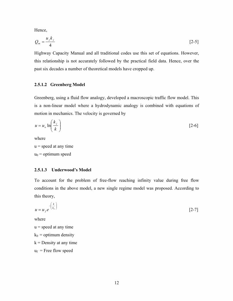
2.5.1.2 Greenberg Model

Greenberg, using a fluid flow analogy, developed a macroscopic traffic flow model. This

is a non-linear model where a hydrodynamic analogy is combined with equations of

motion in mechanics. The velocity is governed by

=

kk

uu jo ln [2-6]

where

u = speed at any time

u0 = optimum speed

2.5.1.3 Underwood’s Model To account for the problem of free-flow reaching infinity value during free flow

conditions in the above model, a new single regime model was proposed. According to

this theory,

−

= okk

f euu [2-7]

where

u = speed at any time

k0 = optimum density

k = Density at any time

uf = Free flow speed

12

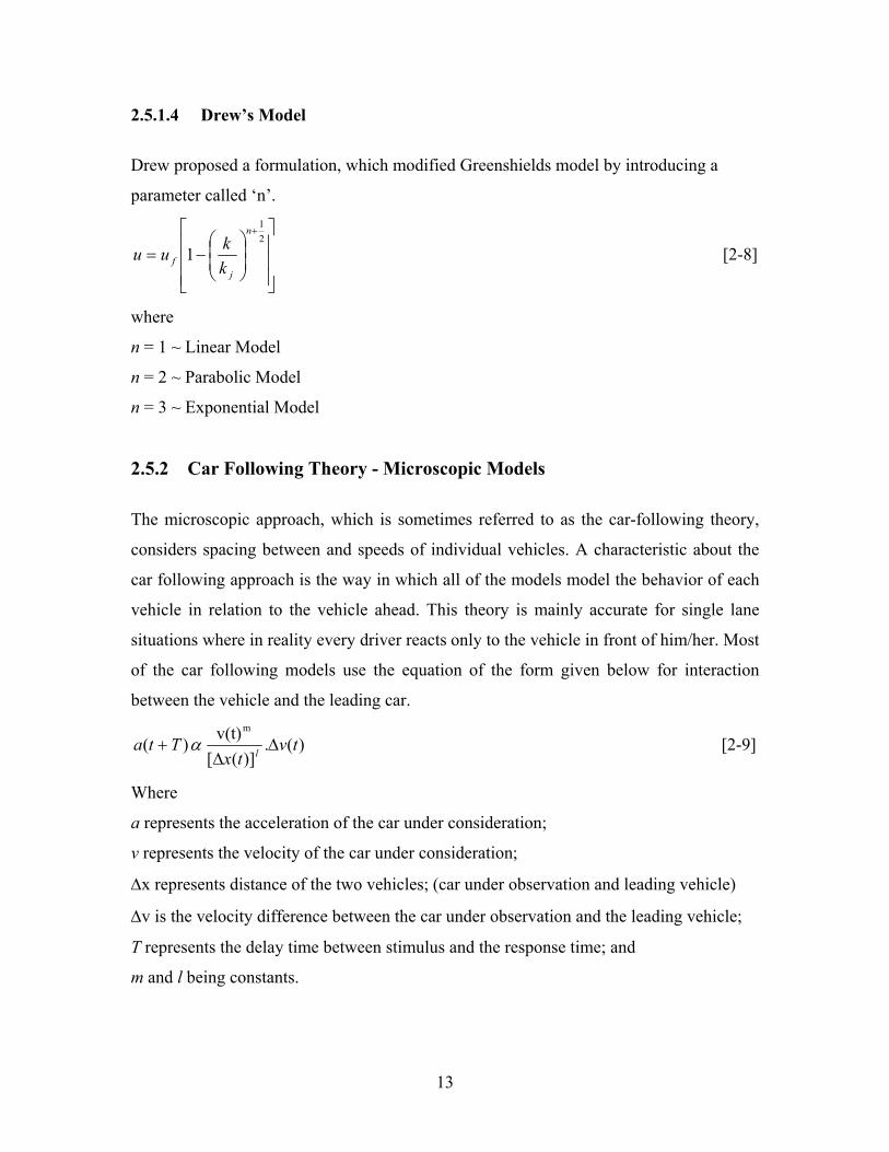
2.5.1.4 Drew’s Model

Drew proposed a formulation, which modified Greenshields model by introducing a

parameter called ‘n’.

−=

+21

1n

jf k

kuu [2-8]

where

n = 1 ~ Linear Model

n = 2 ~ Parabolic Model

n = 3 ~ Exponential Model

2.5.2 Car Following Theory - Microscopic Models

The microscopic approach, which is sometimes referred to as the car-following theory,

considers spacing between and speeds of individual vehicles. A characteristic about the

car following approach is the way in which all of the models model the behavior of each

vehicle in relation to the vehicle ahead. This theory is mainly accurate for single lane

situations where in reality every driver reacts only to the vehicle in front of him/her. Most

of the car following models use the equation of the form given below for interaction

between the vehicle and the leading car.

)(.)]([

v(t) )(m

tvtx

Tta l ∆∆

+ α [2-9]

Where

a represents the acceleration of the car under consideration;

v represents the velocity of the car under consideration;

∆x represents distance of the two vehicles; (car under observation and leading vehicle)

∆v is the velocity difference between the car under observation and the leading vehicle;

T represents the delay time between stimulus and the response time; and

m and l being constants.

13

Theories describing how one vehicle follows another vehicle were developed primarily in

the 1950s and 1960s. Reuschel and Pipes were pioneers in the development of car

following theories in early 1950s.Three parallel efforts were undertaken in the late 1950s

and continued to the mid 1960s. Kometani and sasaki in Japan, Forbes at the Institute for

Research and Michigan state University and a group of researchers associated with

General Motors made significant contributions to car following theory. There were a

series of car following theories proposed by professor Adolph May, 1990 in publication “

traffic flow theory”. The basic form of these theories was:

Response = f{sensitivity, Stimuli}

where

Response = Acceleration or Deceleration of the vehicle which is dependent on the

sensitivity of the automobile and the driver himself

Sensitivity = Ability of the driver to perceive and react to the stimuli

Stimuli = Visual and auditory inputs that influence driver’s decision

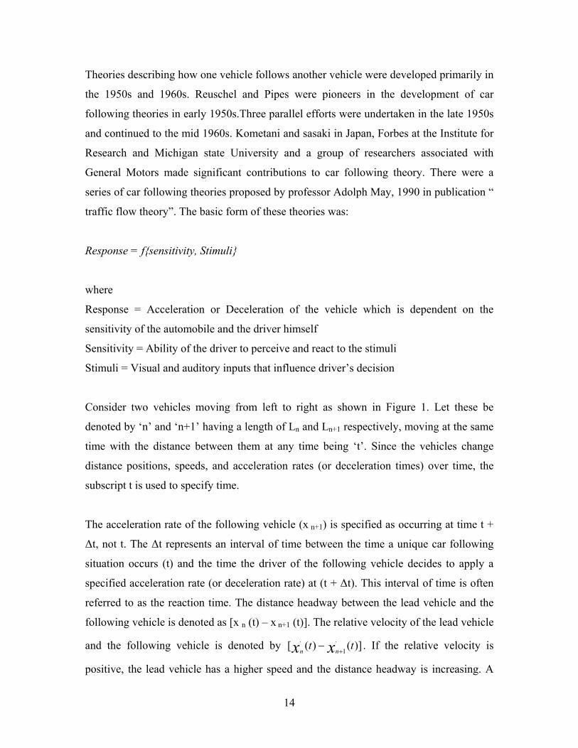
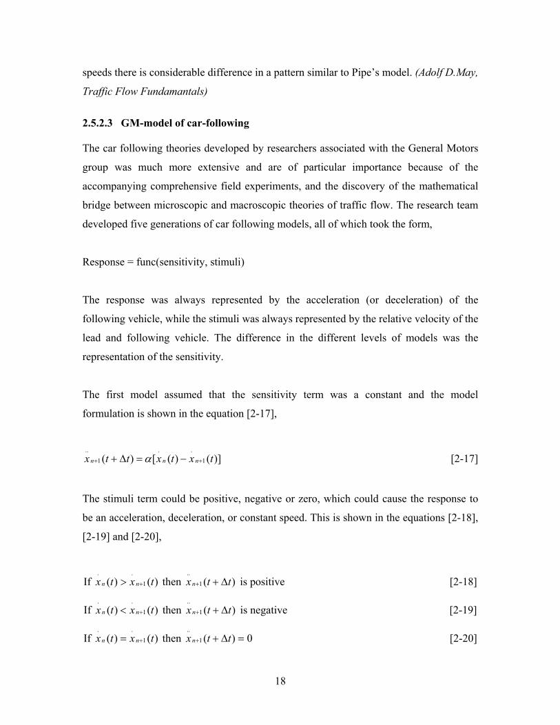
Consider two vehicles moving from left to right as shown in Figure 1. Let these be

denoted by ‘n’ and ‘n+1’ having a length of Ln and Ln+1 respectively, moving at the same

time with the distance between them at any time being ‘t’. Since the vehicles change

distance positions, speeds, and acceleration rates (or deceleration times) over time, the

subscript t is used to specify time.

The acceleration rate of the following vehicle (x n+1) is specified as occurring at time t +

∆t, not t. The ∆t represents an interval of time between the time a unique car following

situation occurs (t) and the time the driver of the following vehicle decides to apply a

specified acceleration rate (or deceleration rate) at (t + ∆t). This interval of time is often

referred to as the reaction time. The distance headway between the lead vehicle and the

following vehicle is denoted as [x n (t) – x n+1 (t)]. The relative velocity of the lead vehicle

and the following vehicle is denoted by [ . If the relative velocity is

positive, the lead vehicle has a higher speed and the distance headway is increasing. A

)]()( .

1

. tt xx nn +−

14

negative value implies that the following vehicle has a higher speed and the distance

headway is decreasing. Finally, the acceleration rate (or deceleration rate) [

can be positive or negative, with a positive value indicating that the following vehicle is

accelerating and increasing its speed while a negative value indicates the reverse. (Adolf

D.May, Traffic Flow Fundamantals)

)](..

1ttxn

∆++

Figure 1: A Car Following Theory

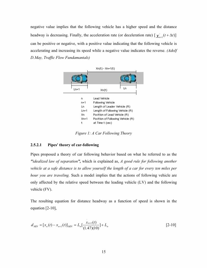
2.5.2.1 Pipes' theory of car-following

Pipes proposed a theory of car following behavior based on what he referred to as the

"idealized law of separation”, which is explained as, A good rule for following another

vehicle at a safe distance is to allow yourself the length of a car for every ten miles per

hour you are traveling. Such a model implies that the actions of following vehicle are

only affected by the relative speed between the leading vehicle (LV) and the following

vehicle (FV).

The resulting equation for distance headway as a function of speed is shown in the

equation [2-10],

nn

nMINnnMIN LtxLtxtxd +=−= ++ ]

)10)(47.1()([)]()([ 1

.

1 [2-10]

15

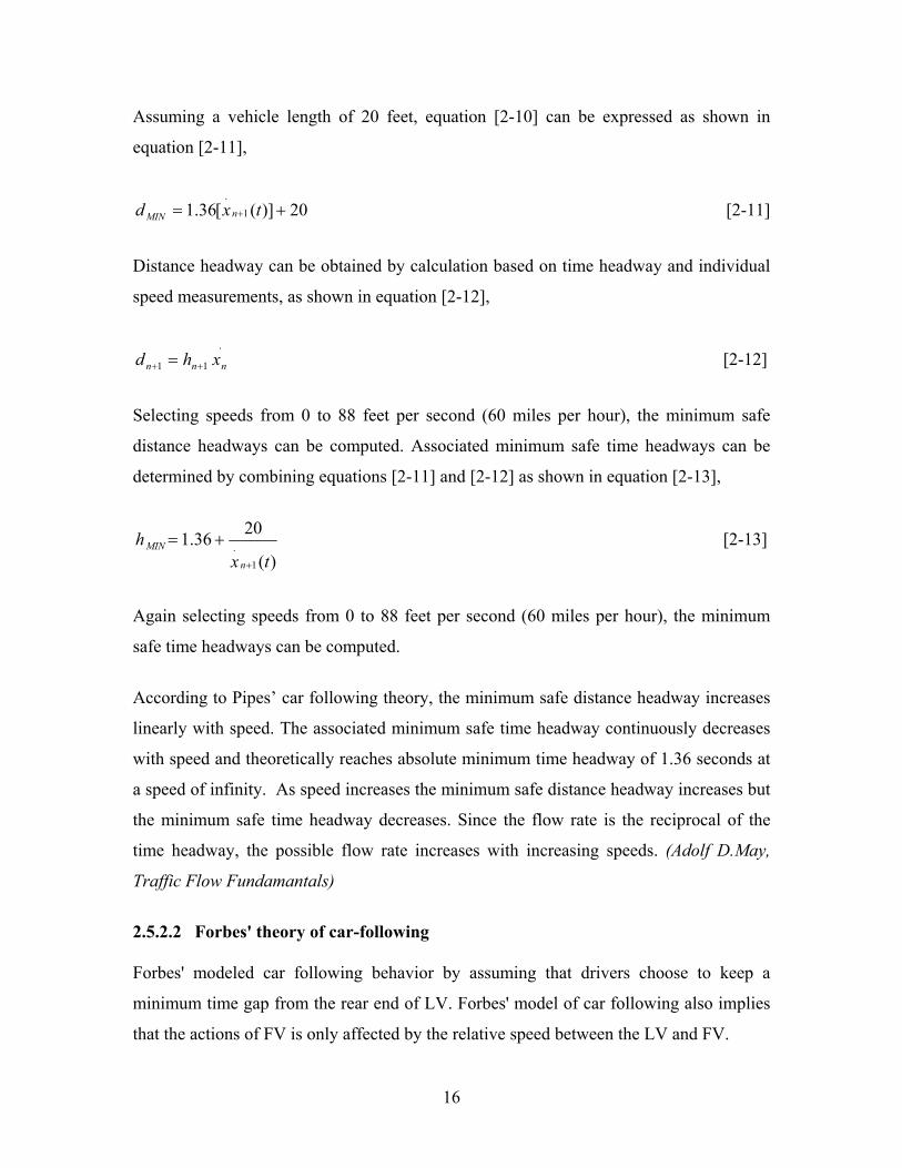
Assuming a vehicle length of 20 feet, equation [2-10] can be expressed as shown in

equation [2-11],

20)]([36.1 1

.+= + txd nMIN [2-11]

Distance headway can be obtained by calculation based on time headway and individual

speed measurements, as shown in equation [2-12],

.

11 nnn xhd ++ = [2-12]

Selecting speeds from 0 to 88 feet per second (60 miles per hour), the minimum safe

distance headways can be computed. Associated minimum safe time headways can be

determined by combining equations [2-11] and [2-12] as shown in equation [2-13],

)(

2036.11

.tx

hn

MIN

+

+= [2-13]

Again selecting speeds from 0 to 88 feet per second (60 miles per hour), the minimum

safe time headways can be computed.

According to Pipes’ car following theory, the minimum safe distance headway increases

linearly with speed. The associated minimum safe time headway continuously decreases

with speed and theoretically reaches absolute minimum time headway of 1.36 seconds at

a speed of infinity. As speed increases the minimum safe distance headway increases but

the minimum safe time headway decreases. Since the flow rate is the reciprocal of the

time headway, the possible flow rate increases with increasing speeds. (Adolf D.May,

Traffic Flow Fundamantals)

2.5.2.2 Forbes' theory of car-following

Forbes' modeled car following behavior by assuming that drivers choose to keep a

minimum time gap from the rear end of LV. Forbes' model of car following also implies

that the actions of FV is only affected by the relative speed between the LV and FV.

16

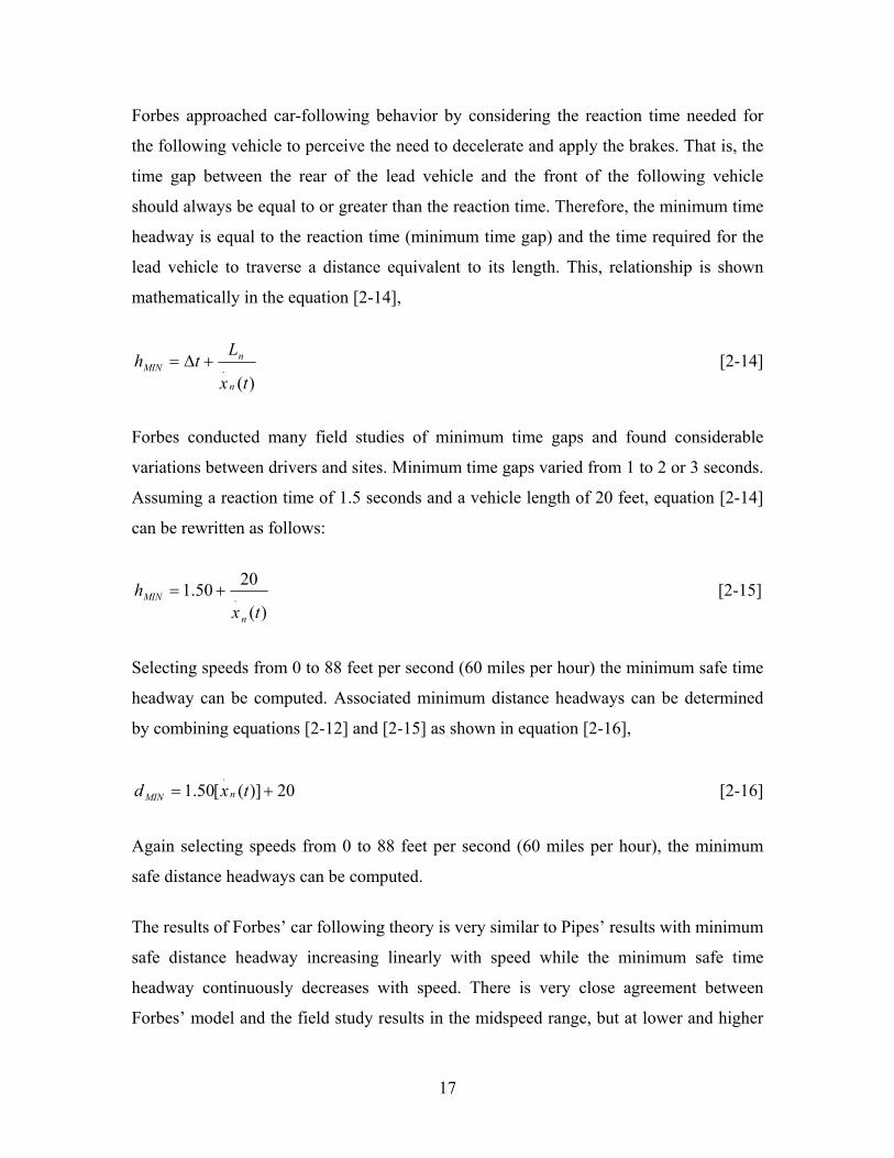
Forbes approached car-following behavior by considering the reaction time needed for

the following vehicle to perceive the need to decelerate and apply the brakes. That is, the

time gap between the rear of the lead vehicle and the front of the following vehicle

should always be equal to or greater than the reaction time. Therefore, the minimum time

headway is equal to the reaction time (minimum time gap) and the time required for the

lead vehicle to traverse a distance equivalent to its length. This, relationship is shown

mathematically in the equation [2-14],

)(.

tx

Lth

n

nMIN +∆= [2-14]

Forbes conducted many field studies of minimum time gaps and found considerable

variations between drivers and sites. Minimum time gaps varied from 1 to 2 or 3 seconds.

Assuming a reaction time of 1.5 seconds and a vehicle length of 20 feet, equation [2-14]

can be rewritten as follows:

)(

2050.1 .tx

hn

MIN += [2-15]

Selecting speeds from 0 to 88 feet per second (60 miles per hour) the minimum safe time

headway can be computed. Associated minimum distance headways can be determined

by combining equations [2-12] and [2-15] as shown in equation [2-16],

20)]([50.1.

+= txd nMIN [2-16]

Again selecting speeds from 0 to 88 feet per second (60 miles per hour), the minimum

safe distance headways can be computed.

The results of Forbes’ car following theory is very similar to Pipes’ results with minimum

safe distance headway increasing linearly with speed while the minimum safe time

headway continuously decreases with speed. There is very close agreement between

Forbes’ model and the field study results in the midspeed range, but at lower and higher

17

speeds there is considerable difference in a pattern similar to Pipe’s model. (Adolf D.May,

Traffic Flow Fundamantals)

2.5.2.3 GM-model of car-following The car following theories developed by researchers associated with the General Motors

group was much more extensive and are of particular importance because of the

accompanying comprehensive field experiments, and the discovery of the mathematical

bridge between microscopic and macroscopic theories of traffic flow. The research team

developed five generations of car following models, all of which took the form,

Response = func(sensitivity, stimuli)

The response was always represented by the acceleration (or deceleration) of the

following vehicle, while the stimuli was always represented by the relative velocity of the

lead and following vehicle. The difference in the different levels of models was the

representation of the sensitivity.

The first model assumed that the sensitivity term was a constant and the model

formulation is shown in the equation [2-17],

)]()([)( 1

..

1

..txtxttx nnn ++ −=∆+ α [2-17]

The stimuli term could be positive, negative or zero, which could cause the response to

be an acceleration, deceleration, or constant speed. This is shown in the equations [2-18],

[2-19] and [2-20],

If then is positive [2-18] )()( 1

..txtx nn +> )(1

..ttxn ∆++

If then is negative [2-19] )()( 1

..txtx nn +< )(1

..ttxn ∆++

If then [2-20] )()( 1

..txtx nn += 0)(1

..=∆++ ttxn

18

Field experiments were conducted on the General Motors test track to quantify the

parameter values for the reaction time (∆t) and the sensitivity parameter (α). The

significant range in the sensitivity value alerted the investigators that the spacing between

vehicles should be introduced into the sensitivity term. This led to the development of the

second model, which proposed that the sensitivity term should have two states. That is,

when the two vehicles were close together, a high sensitivity value (α2) should be used.

This formulation can be shown by equation [2-21],

)]()([)( 1

..

1

.. 1

2

txtxttx nnn ++ −∫=∆+α

α

[2-21]

Very quickly the investigators saw the difficulty in selecting the α1 and α2 values and the

difficulty associated with discontinuous states. This led to further field experiments to

determine means of incorporating the distance headway, into the sensitivity term. The

relationship was determined for αo, d, and α as shown in the equation [2-22],

ddo ααα ==

1 [2-22]

)()( 1

0

txtxd nn

o

+−==

ααα [2-23]

Then equation [2-23] for α was substituted into equation [2-17], and the third model

resulted as shown in the equation [2-24].

)]()([)()(

)( 1

..

1

1

..txtx

txtxttx nn

nn

on +

+

+ −−

=∆+α

[2-24]

The fourth model was a further development towards improving the sensitivity term by

introducing the speed of the following vehicle. The concept was that as the speed of the

traffic stream increased, the driver of the following vehicle would be more sensitive to

19

the relative velocity between the lead and following vehicle. The formulation of this

fourth model is shown in the equation [2-25],

)]()([)()()]([')( 1

..

1

1

.

1

..txtx

txtxttxttx nn

nn

nn +

+

++ −

−∆+

=∆+α [2-25]

where

α′ = Speed of the following vehicle

The fifth and the final model was a continued effort to improve and generalize the

sensitivity term. The question was raised whether the speed and distance headway

components should be raised to the first power or whether an improved and more

generalized approach could be accomplished by introducing generalized exponents. This

was implemented by introducing m and l exponents as shown in the equation [2-26],

)()([)]()([)]([

)( 1

..

1

1,1

.txtx

txtxttx

ttx nnlnn

mnml

n +

+

+

⋅

+ −−

∆+=∆+

α] [2-26]

where

m = Speed exponent

l = Distance headway

Ranges of values: m = -2 to 2 and l = -1 to 4

It can be found that upon substitution of different combinations of m and 1 terms, the

resultant microscopic general motors formulae take the shape of various macroscopic

models, proposed by various researchers. The model is widely accepted as a generalized

car following model, which can be modified and applied to a particular case. (Adolf

D.May, Traffic Flow Fundamantals)

2.5.3 Particle Hopping Theory – Mesoscopic Model

This is one of the approaches for modeling traffic. Considering a one-dimensional chain

of cells, each cell either empty, or occupied by exactly one particle, movement of

particles is achieved by particles jumping from one cell to another according to specific

movement rules. In the context of vehicular traffic, one can imagine a road represented

20

by cells, which can fit exactly one car. A rough representation of car movements then is

given by moving cars from one cell to another.

In general all particle-hopping models are defined on a lattice. The lattice being made up

of a certain number of sites, each of which is either empty or occupied by a particle.

Another characteristic of the model is that only one particle can occupy each site and all

the movement of these particles is to be in one direction. This model adheres to the laws

of conservation of total mass, which states that the total particles in the system are

conserved except at boundaries where particles can either enter or exit. In traffic models

the road segments are generally thought of as a lattice and each vehicle represents

particles. (Nagel, K. et al, LA-UR 96-659). These models are sometimes called cellular

automata (CA). Particle hopping models and CA are not exactly the same, although the

definitions are overlapping.

This section starts out with the Stochastic Traffic Cellular Automaton (STCA), which has

been proposed for traffic flow and which is currently implemented as a microsimulation

option for large scale traffic simulation projects. The STCA includes strong randomness

in the rules. Setting this randomness to zero reduces the STCA to be a much simpler,

deterministic model, which, when restricting oneself to maximum velocity vmax = 1, turns

out to a well-known cellular automaton model. In the third model of this section,

randomness is re-introduced, but in this case by changing the update algorithm: Whereas

in the first two models all particles are updated synchronously based in “old"

information, in this third model, particles are selected in random sequence for individual

updates.

2.5.3.1 The Stochastic Traffic Cellular Automaton (STCA)

The characteristics of the Stochastic Traffic Cellular Automaton are defined below. Each

particle (in traffic sense referring to a vehicle) has a velocity that is either 0 or an integer.

The speed constrained by a maximum of vmax. This means that every vehicle can only

take integer values of velocity between 0 and vmax. The configuration of timestep t+1 is

21

computed from the stored configuration of timestep t, using either parallel or

synchronous updates. The decisions for the timestep t+1 entirely depend on the

configuration at timestep t. Briefed below are the update procedures executed by every

particle/vehicle in parallel. (Nagel,K. et al, LA-UR 95-2098)

The gap ahead of the particle/vehicle is computed •

•

•

•

If the velocity of the particle is greater than the gap, a need for slowing down

the particle is observed and its velocity changed so it

equals the gap ahead. Else if there is enough headway in front of the vehicle

and the vehicle is not moving at the maximum speed allowed then its velocity

is incremented so as to represent acceleration. This acceleration is however

gradual so as to represent daily behavior.

To capture the realistic behavior of traffic, some randomness is introduced.

This models the idea of particles/vehicles slowing down without reason,

fluctuations at maximum speed, overreactions at breaking and noisy

accelerations. For such a condition to occur, the velocity of the particle should

clearly be positive and non-zero. With a probability p, the velocity of such a

particle is thus reduced by one.

Once these decisions have been taken the particle/vehicle is moved ahead

depending on the velocity computed as listed above.

It is interesting to note in this model if the maximum velocity is set to one, i.e., vmax =1,

then the model behaves very differently from what it would when the maximum velocity

is greater than two. All the conditions stated above reduce to a singular statement that

states a particle to move ahead to the next cell with a probability of p, should it be free.

The analysis for STCA/2 (STCA with vmax >= 2) shows that there is a very dynamic and

a different flow regime that does not have an exact solution. Inspection of the space-time

plots visually confirmed that the dynamics of this model was very similar to STCA-CC/2

(which is discussed later) more than to the ASEP (discussed later). It was observed that

multiple jams could exist simultaneously. Jams in such a models start simultaneously and

22

independently of other jams attributed to the velocity fluctuations at maximum speed and

depended on the parameter pfree (not equal to zero).

2.5.3.2 The Deterministic Limit of the STCA (CA-184)

The deterministic limit of the STCA models unprobabilistic nature of the STCA i.e.,

taking the randomness out of the randomness step. This is, when the maximum velocity

equal to one, equivalent to cellular automaton rule 184 in Wolfram’s notation. (Nagel,K.

et al, LA-UR 95-2098) It is interesting to note that most Cellular Automaton Traffic

models are based on this model.

2.5.3.3 The Asymmetric Stochastic Exclusion Process (ASEP)

The Asymmetric Exclusion Process or ASEP for short is probably the most investigated

particle-hopping model. The ASEP models behavior that can be generalized by two

simple rules stated below

Selection of a random particle/vehicle; •

• Movement of the particle to the right should the space on that site be empty.

The ASEP model is closely related to the STCA and CA models that were discussed

earlier. The ASEP model behaves just the same way that STCA/1 and CA-184/1 do. This

is because in rule two of ASEP, particles are only updated to the next site and not further.

The basic difference though between them would be the way in which the particles are

updated.

STCA/1 and CA-184/1 particles are all updated once and synchronously while ASEP

does random updates of particles in a sense that these updates are a random serial

sequence. However comparisons can be made between these models after defining the

quantity timestep for the ASEP model. The definition of a timestep is clear and

understood for the STCA and the CA-184 models as being the time between two

23

successive updates of particles. In ASEP at an average a particle is updated after n single-

particle updates, a timestep is thus completed after N single-particle updates.

It can also be observed that the randomness in the updates of the particles can be reduced

i.e., reduction in the noise by techniques discussed by Wolf and Kertesz. They stated that

using a counter associated with every particle could considerably reduce the noise if the

updates are only made after k trials. It can also be seen that as k increases to a very large

value the ASEP model slowly tends to behave as a CA-184. (Nagel,K. et al, LA-UR 95

2098).

2.6 Specific Characteristics of the Simulation Packages

The vehicle movements with the car following logic, lane changing logic and movements

at the intersections, in all the four simulation models is discussed in the following

sections.

2.6.1 TRANSIMS TRANSIMS is a five-module software package; each module dealing with a specific

task. The modules are Population Synthesizer, Activity Generator, Route Planner,

Microsimulator and a Selector. Another module is the Emissions Estimator, which as the

name suggests calculates the amount of emissions for the region in analysis using the

outputs of the above-mentioned previous five modules.

A very brief description of what each module does is presented next starting with the

Population Synthesizer. This module of TRANSIMS uses the PUMS data and the STF-

3A data provided by the Census to create synthetic population having the same aggregate

characteristics to those in the census data. This module also locates this synthetic

population on transportation network using a suitable algorithm. The Activity Generator

then assigns activities to these synthetic population based on the activity survey data

depending on the household and demographic characteristics using the CART algorithm.

Once the synthetic population is in place with their respective activities the Route Planner

designates to each traveler his travel plans, i.e., how he/she goes about doing his/her

24

activities. Should the activity of synthetic household include activities that require travel

on the transportation network, the Route Planner finds the shortest path using various

shortest path algorithms and assigns the traveler his exact itinerary detailing the links and

nodes he travels on to reach his destination. On having these plans and the transportation

network, the Microsimulator simulates the plans for all travelers on the network, their

movements being governed by some simple rules. The Microsimulator uses a cellular

automata approach for simulating vehicles on the network. Traffic behavior that the

analyst wants to study is collected as the simulation progresses. The selector module

provides the feedback for the whole process so that any unrealistic data such as an

infeasible plan or an unlocatable household can be dealt by redoing his plan or relocating

him with changed household characteristics or demographics.

The TRANSIMS Microsimulator module simulates the movement and the interactions of

travelers in the transportation system of the study area. In this module every traveler tries

to execute his/her travel movements according to plan. These movements and interactions

produce key data that is output from the Microsimulator, bringing about more

macroscopic quantities like volume, flow etc by aggregation of these individual

interactions. The Microsimulator imitates realistic traffic behavior in decisions about lane

changes, passing slow vehicles and evaluating interactions with other vehicles. As this

research mainly deals with analyzing weaving areas, it is noted that the Microsimulator is

the only module that affects it. (Jillella et al., 2001)

This section highlights how the Microsimulator conducts the movements of the travelers

encompassing vehicle movements, lane changes and traversal across intersections.

2.6.1.1 Vehicle Movement In The Same Lane

Vehicles in the TRANSIMS network follow simple rules that govern their movements.

These rules are intentionally kept simple to enhance the computation speed considering

the millions of interactions taking place in the system. At the core, the rules for a vehicle

25

movement in the same lane could be put simply as “Acceleration whenever possible,

Deceleration only if necessary and sometimes for no reason”.

The decision by a vehicle to accelerate or decelerate depends on its current speed, and the

gap between it and the immediate vehicle ahead in the same lane. Another factor that

influences the movement of a vehicle is the deceleration probability (Pd), which can be

thought of as the probability of a vehicle decelerating in the timestep. All the vehicles in

the TRANSIMS network are constrained by a maximum attainable speed that is specified

(VGlobalMax, which is 5 cells/timestep or about 80 mph).

Consider a vehicle traveling at a certain speed at a given timestep. Now if the vehicle

speed is greater than the gap ahead, the vehicle needs to reduce its speed to avoid a

collision. The amount of deceleration being subject to, depends on how large or small the

current gap (Gc) is compared to the current speed. To model aggressive breaking an

element of randomness in the form of Pd is used. If the probability of decelerating is

greater than a certain threshold value (Pnoise), the speed of the vehicle is further reduced

than what can be actually attainable based on gap (Gc). Considering the scenario where

the gap ahead of the vehicle is larger than its current speed, then the vehicle can possibly

accelerate. The magnitude of acceleration is specified differently for each type of vehicle.

All velocity and acceleration changes are integer values based on the number of

cells/second or cells/second/second respectively.

In the case that the vehicle is traveling at maximum allowable speed and having enough

gap ahead to accelerate, the vehicle stays at maximum speed. As explained earlier the

probability for deceleration is randomly activated and the vehicles speed may be reduced

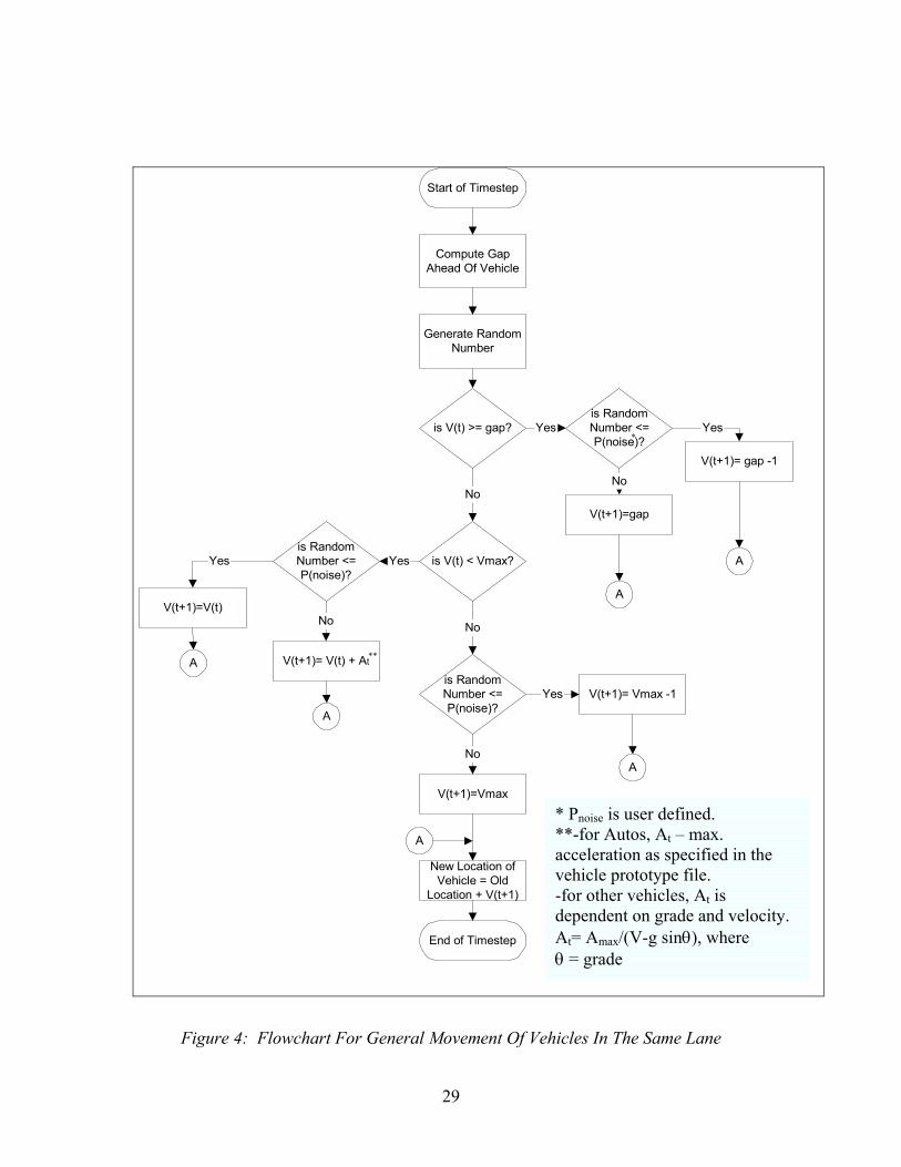
by 1 cell/second. A flowchart, illustrating the logic for the vehicles movement in the

same lane, is outlined in Figure 4.

To illustrate the above rules for general movement in a lane, the following pictorial

examples on speeds are provided including their calculations.

26

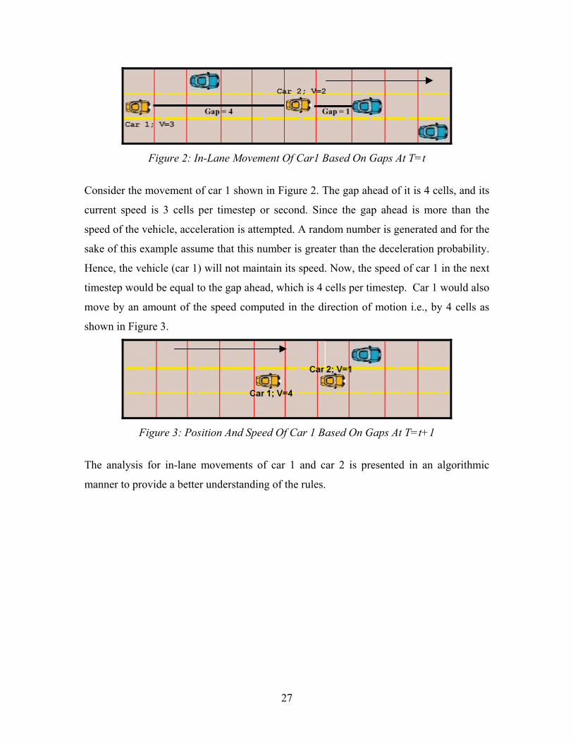
Figure 2: In-Lane Movement Of Car1 Based On Gaps At T=t

Consider the movement of car 1 shown in Figure 2. The gap ahead of it is 4 cells, and its

current speed is 3 cells per timestep or second. Since the gap ahead is more than the

speed of the vehicle, acceleration is attempted. A random number is generated and for the

sake of this example assume that this number is greater than the deceleration probability.

Hence, the vehicle (car 1) will not maintain its speed. Now, the speed of car 1 in the next

timestep would be equal to the gap ahead, which is 4 cells per timestep. Car 1 would also

move by an amount of the speed computed in the direction of motion i.e., by 4 cells as

shown in Figure 3.

Figure 3: Position And Speed Of Car 1 Based On Gaps At T=t+1

The analysis for in-lane movements of car 1 and car 2 is presented in an algorithmic

manner to provide a better understanding of the rules.

27

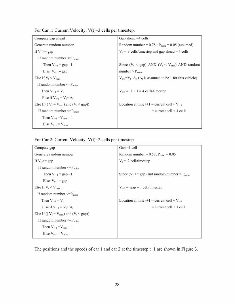
For Car 1: Current Velocity, V(t)=3 cells per timestep.

Compute gap ahead

Generate random number

If Vt >= gap

If random number <=Pnoise

Then Vt+1 = gap –1

Else Vt+1 = gap

Else If Vt < Vmax

If random number <=Pnoise

Then Vt+1 = Vt

Else if Vt+1 = Vt+ At

Else If (( Vt = Vmax) and (Vt < gap))

If random number <=Pnoise

Then Vt+1 =Vmax – 1

Else Vt+1 = Vmax

Gap ahead =4 cells

Random number = 0.78 ; Pnoise = 0.05 (assumed)

Vt = 3 cells/timestep and gap ahead = 4 cells

Since (Vt < gap) AND (Vt < Vmax) AND random

number > Pnoise

Vt+1=Vt+At (At is assumed to be 1 for this vehicle)

Vt+1 = 3 + 1 = 4 cells/timestep

Location at time t+1 = current cell + Vt+1

= current cell + 4 cells

For Car 2: Current Velocity, V(t)=2 cells per timestep

Compute gap

Generate random number

If Vt >= gap

If random number <=Pnoise

Then Vt+1 = gap –1

Else Vt+1 = gap

Else If Vt < Vmax

If random number <=Pnoise

Then Vt+1 = Vt

Else if Vt+1 = Vt+ At

Else If (( Vt = Vmax) and (Vt < gap))

If random number <=Pnoise

Then Vt+1 =Vmax – 1

Else Vt+1 = Vmax

Gap =1 cell

Random number = 0.57; Pnoise = 0.05

Vt = 2 cell/timestep

Since (Vt >= gap) and random number > Pnoise

Vt+1 = gap = 1 cell/timestep

Location at time t+1 = current cell + Vt+1

= current cell + 1 cell

The positions and the speeds of car 1 and car 2 at the timestep t+1 are shown in Figure 3.

28

Start of Timestep

Compute GapAhead Of Vehicle

Generate RandomNumber

is V(t) >= gap?is RandomNumb <=P(noi )?

is V(t) < Vmax?is RandomNumber <=P(noise)?

is RandomNumber <=P(noise)?

V(t+1)

V(t+1)

V(t+1)=Vmax

V(t+1)=V(t)

V(t+1)= V(t) + A

Yes

Yes

Yes

Yes

Yes

NoNo

NoNo

No

A

A

A

End of Timestep

A

New Location ofVehicle = Old

Location + V(t+1)

* Pnoise is **-for Auaccelerativehicle pr-for otherdependenAt= Amax/θ = grade

*

Figure 4: Flowchart For General Movement Of Vehicles In T

29

erse

V(t+1)= gap -1

=gap

A

t**

= Vmax -1

A

user defined. tos, At – max. on as specified in the ototype file. vehicles, At is t on grade and velocity. (V-g sinθ), where

he Same Lane

2.6.1.2 Lane Changing logic

The lane-changing maneuver of a vehicle in TRANSIMS Microsimulator occurs to pass a

slower vehicle immediately ahead or to make turns at intersections following its current

plan. The decisions for lane changes take place before the in-lane movement of the

vehicles on the links occur. This ensures that the in-lane movement of the vehicles takes

into account the effect of lane changes.

Lane changes into the left lane and into the right lane are treated by the Microsimulator

on alternating timesteps. The left lane changes are made on even timesteps while the right

ones are made on odd timesteps. Multilane roadways are processed from left to the right

during left lane changing and from the right to the left during right lane changing

procedures. It should be noted that these lane change procedures are only explored if the

cell on the adjacent lane in which the vehicle is trying to change into is vacant.

The above mentioned lane changing procedures are discussed in detail below under two

separate categories. One category is for lane changing based purely on passing a slower

vehicle, and the other one is based on making turns at intersections to follow plan.

Lane changes based on passing slower vehicles

The lane changes based on this criterion occur only if the speed of the vehicle under

consideration is more than or equal to the gap ahead of it in the current lane (Gc). Another

important consideration is the magnitude of the gaps in the adjacent lane to which the

vehicle is attempting a lane change into. The gap ahead of the vehicle in the new adjacent

lane (Gf) should be larger than the one in the current lane (Gc). The vehicle, before

making the necessary lane change, should also consider if the vehicle behind it in the new

lane is sufficiently far away (Gb) to avoid any kind of collision.

The above ideas are captured into the TRANSIMS Microsimulator using three variables

Weight1, Weight2 and Weight 3. The values of these weights are computed as shown in

30

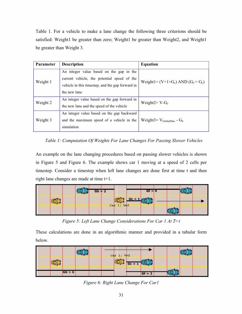
Table 1. For a vehicle to make a lane change the following three criterions should be

satisfied: Weight1 be greater than zero; Weight1 be greater than Weight2, and Weight1

be greater than Weight 3.

Parameter Description Equation

Weight 1

An integer value based on the gap in the

current vehicle, the potential speed of the

vehicle in this timestep, and the gap forward in

the new lane

Weight1= (V+1>Gc) AND (Gf > Gc)

Weight 2 An integer value based on the gap forward in

the new lane and the speed of the vehicle Weight2= V-Gf

Weight 3 An integer value based on the gap backward

and the maximum speed of a vehicle in the

simulation

Weight3= VGlobalMax - Gb

Table 1: Computation Of Weights For Lane Changes For Passing Slower Vehicles

An example on the lane changing procedures based on passing slower vehicles is shown

in Figure 5 and Figure 6. The example shows car 1 moving at a speed of 2 cells per

timestep. Consider a timestep when left lane changes are done first at time t and then

right lane changes are made at time t+1.

Figure 5: Left Lane Change Considerations For Car 1 At T=t

These calculations are done in an algorithmic manner and provided in a tabular form

below.

Figure 6: Right Lane Change For Car1

31

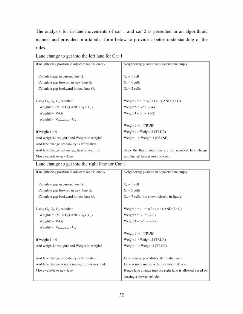
The analysis for in-lane movements of car 1 and car 2 is presented in an algorithmic

manner and provided in a tabular form below to provide a better understanding of the

rules.

Lane change to get into the left lane for Car 1 If neighboring position in adjacent lane is empty

Calculate gap in current lane Gc

Calculate gap forward in new lane Gf

Calculate gap backward in new lane Gb

Using Gc, Gf, Gb calculate

Weight1= (V+1>Gc) AND (Gf > Gc)

Weight2= V-Gf

Weight3= VGlobalMax - Gb

If weight 1 > 0

And weight1> weight2 and Weight1> weight3

And lane change probability is affirmative

And lane change not merge, turn or next link

Move vehicle to new lane

Neighboring position in adjacent lane empty

Gc = 1 cell

Gf = 4 cells

Gb = 2 cells

Weight1 = 1 = ((2+1 > 1) AND (4>1))

Weight2 = -2 = (2-4)

Weight3 = 3 = (5-2)

Weight1 =1 (TRUE)

Weight1 > Weight 2 (TRUE)

Weight 1 > Weight 3 (FALSE)

Since the three conditions are not satisfied, lane change

into the left lane is not allowed.

Lane change to get into the right lane for Car 1 If neighboring position in adjacent lane is empty

Calculate gap in current lane Gc

Calculate gap forward in new lane Gf

Calculate gap backward in new lane Gb

Using Gc, Gf, Gb calculate

Weight1= (V+1>Gc) AND (Gf > Gc)

Weight2= V-Gf

Weight3= VGlobalMax - Gb

If weight 1 > 0

And weight1> weight2 and Weight1> weight3

And lane change probability is affirmative

And lane change is not a merge, turn or next link

Move vehicle to new lane

Neighboring position in adjacent lane empty

Gc = 1 cell

Gf = 3 cells

Gb = 7 cells (not shown clearly in figure)

Weight1 = 1 = ((2+1 > 1) AND (3>1))

Weight2 = -1 = (2-3)

Weight3 = -2 = (5-7)

Weight1 =1 (TRUE)

Weight1 > Weight 2 (TRUE)

Weight 1 > Weight 3 (TRUE)

Lane change probability affirmative and

Lane is not a merge or turn or next link one.

Hence lane change into the right lane is allowed based on

passing a slower vehicle.

32

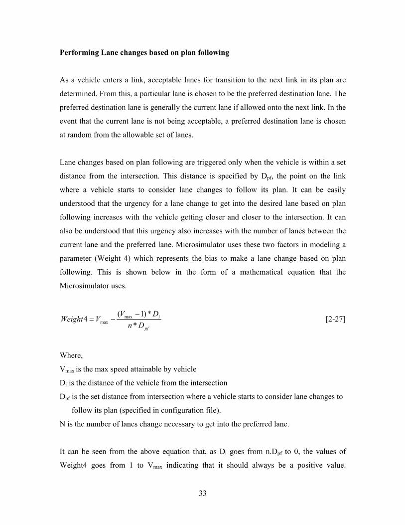
Performing Lane changes based on plan following

As a vehicle enters a link, acceptable lanes for transition to the next link in its plan are

determined. From this, a particular lane is chosen to be the preferred destination lane. The

preferred destination lane is generally the current lane if allowed onto the next link. In the

event that the current lane is not being acceptable, a preferred destination lane is chosen

at random from the allowable set of lanes.

Lane changes based on plan following are triggered only when the vehicle is within a set

distance from the intersection. This distance is specified by Dpf, the point on the link

where a vehicle starts to consider lane changes to follow its plan. It can be easily

understood that the urgency for a lane change to get into the desired lane based on plan

following increases with the vehicle getting closer and closer to the intersection. It can

also be understood that this urgency also increases with the number of lanes between the

current lane and the preferred lane. Microsimulator uses these two factors in modeling a

parameter (Weight 4) which represents the bias to make a lane change based on plan

following. This is shown below in the form of a mathematical equation that the

Microsimulator uses.

pf

i

DnDV

VWeight*

*)1(4 max

max−

−= [2-27]

Where,

Vmax is the max speed attainable by vehicle

Di is the distance of the vehicle from the intersection

Dpf is the set distance from intersection where a vehicle starts to consider lane changes to

follow its plan (specified in configuration file).

N is the number of lanes change necessary to get into the preferred lane.

It can be seen from the above equation that, as Di goes from n.Dpf to 0, the values of

Weight4 goes from 1 to Vmax indicating that it should always be a positive value.

33

Weight4 is initially set to 0. However if it is set to –1, it will prevent any passing lane

changes based on gaps. As discussed earlier, left and right lane changes occur on

alternating timesteps even for lane changes based on plan following.

The overall decision to change lane considers both plan following and gaps. The

parameters are adjusted to reflect these conditions.

Weight1 = Weight1 (based on Gaps) + Weight 4.

The overall conditions for lane change remain the same as those based on passing slower

vehicles i.e., Weight1 >0; Weight 1> Weight 2 and Weight 1 > Weight 3.

Figure 7: Example For Lane Change Based On Plan Following

An illustration of a lane change based on plan following is shown in Figure 7. In this

example, the analysis for lane change is presented for Car 1, which is moving with a

velocity of 2 cells per timestep. Let us assume at this point that this vehicle needs to make

a left turn at the intersection, and hence needs to get into the left pocket lane. To get into

the left pocket lane, two left lane changes need to occur i.e., n=2. It can also be clearly

seen that car 1 is 4 cells away from the intersection or Di = 4. For this particular example

34

let us also consider that the lane change for plan following in considered when a vehicle

is within 7 cells from the intersection i.e., Dpf = 7 cells. Taking into consideration all

these factors, Weight 4 is calculated using the equation defined earlier.

pf

i

DnDVVWeight

**)1(4 max

max−

−= [2-28]

= 5 – (5-1)*4/(2*7) =5- 1.14 = 3.87

Using Weight 4, Weight 1 is calculated as Weight1 = Weight 1 + Weight 4; The analysis

then continues exactly as that for lane change based on gaps. For Example;

Weight 1 = 1+3.87 = 4.87

Weight 2 = 2 –3 = -1

Weight 3 = 5 –5 = 0

Since Weight 1>0, and Weight 1> Weight 2, and Weight 1 > Weight 3, the lane change

into the adjacent lane is approved. It is important to note that a car making 2 lane changes

to reach its desired plan following lane, it needs to calculate again Weight 4 and the other

three weights at timestep t+1, after the in-lane movement in the adjacent lane is carried in

this timestep. For this example, the car needs to execute a turn pocket lane change at time

t+1.

35

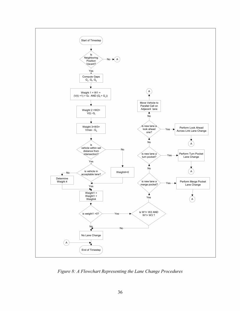
Start of Timestep

IsNeighboring

PositionVacant?

Compute GapsGc, Gf, Gb

Weight 1 = W1 =(V(t) +1) > Gc AND (Gf > Gc))

Weight 2 =W2=V(t) -Gf

Weight 3=W3=Vmax - Gb

isvehicle within set

distance fromintersection?

is vehicle inacceptable lane?

DetermineWeight 4

Weight1 =Weight1 +Weight4

is weight1 >0? is W1> W2 ANDW1> W3 ?

is new lane amerge pocket?

is new lane aturn pocket?

is new lane alook ahead

one?

Perform Turn PocketLane Change

No Lane Change

End of Timestep

Move Vehicle toParallel Cell onAdjacent lane

No

Yes

Yes

No

No

No

Yes

Yes

Yes

No

Yes

No

A

A

Yes

No

Yes

No A

A

A

A

Perform Look AheadAcross Link Lane Change

Perform Merge PocketLane Change

Weight4=0

Figure 8: A Flowchart Representing the Lane Change Procedures

36

2.6.1.3 Vehicle Movements at Intersections

TRANSIMS Microsimulator uses a separate set of rules to model the vehicles leaving a

link and passing through an intersection. Every vehicle arriving at an intersection,

determines a destination lane on the next link onto which it will travel considering the

lane use and HOV restrictions. By default the current lane is chosen if allowed on the

next link, else a lane is picked randomly from the set of allowable lanes.

Vehicles at signalized intersections have different behaviors from those at unsignalized

intersections. The Microsimulator handles vehicles differently at signalized and

unsignalized intersections, though they share some common features. This section

presents the way the Microsimulator handles both these cases. But first, the six conditions

to be satisfied for a vehicle to enter an intersection are provided below.

Condition One: The vehicle has to be the first one on the link going toward the

intersection. This is necessary since the Microsimulator allows only one vehicle per lane

to enter an intersection in a single timestep.

Condition Two: The speed of the vehicle trying to enter the intersection must be greater

than or equal to the number of empty cells between it and the end of the link.

Condition Three: The vehicle entering the intersection should satisfy the conditions of the

traffic control at the intersection. The state of the Traffic Control indicates if a vehicle

must consider oncoming traffic gaps. This would ensure that a vehicle facing a red does

not enter the intersection. For unsignalized intersections the traffic control would specify

a condition of yield or stop. For signalized intersections it would represent a protected,

permitted, or a wait traffic control state. This would specify if the oncoming traffic has to

be considered for an entry into the intersection. The traffic controls and conditions at an

intersection are shown in Table 2.

37

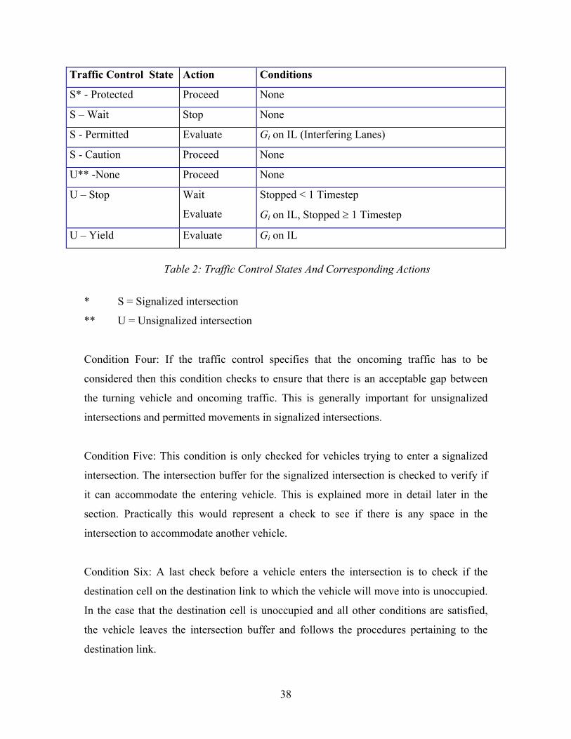
Traffic Control State Action Conditions

S* - Protected Proceed None

S – Wait Stop None

S - Permitted Evaluate Gi on IL (Interfering Lanes)

S - Caution Proceed None

U** -None Proceed None

U – Stop Wait

Evaluate

Stopped < 1 Timestep

Gi on IL, Stopped ≥ 1 Timestep

U – Yield Evaluate Gi on IL

Table 2: Traffic Control States And Corresponding Actions

* S = Signalized intersection

** U = Unsignalized intersection

Condition Four: If the traffic control specifies that the oncoming traffic has to be

considered then this condition checks to ensure that there is an acceptable gap between

the turning vehicle and oncoming traffic. This is generally important for unsignalized

intersections and permitted movements in signalized intersections.

Condition Five: This condition is only checked for vehicles trying to enter a signalized

intersection. The intersection buffer for the signalized intersection is checked to verify if

it can accommodate the entering vehicle. This is explained more in detail later in the

section. Practically this would represent a check to see if there is any space in the

intersection to accommodate another vehicle.

Condition Six: A last check before a vehicle enters the intersection is to check if the

destination cell on the destination link to which the vehicle will move into is unoccupied.

In the case that the destination cell is unoccupied and all other conditions are satisfied,

the vehicle leaves the intersection buffer and follows the procedures pertaining to the

destination link.

38

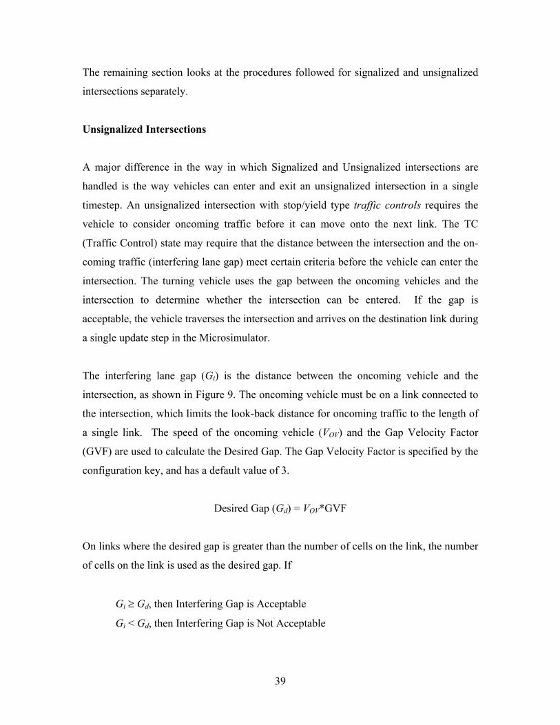
The remaining section looks at the procedures followed for signalized and unsignalized

intersections separately.

Unsignalized Intersections

A major difference in the way in which Signalized and Unsignalized intersections are

handled is the way vehicles can enter and exit an unsignalized intersection in a single

timestep. An unsignalized intersection with stop/yield type traffic controls requires the

vehicle to consider oncoming traffic before it can move onto the next link. The TC

(Traffic Control) state may require that the distance between the intersection and the on-

coming traffic (interfering lane gap) meet certain criteria before the vehicle can enter the

intersection. The turning vehicle uses the gap between the oncoming vehicles and the

intersection to determine whether the intersection can be entered. If the gap is

acceptable, the vehicle traverses the intersection and arrives on the destination link during

a single update step in the Microsimulator.

The interfering lane gap (Gi) is the distance between the oncoming vehicle and the

intersection, as shown in Figure 9. The oncoming vehicle must be on a link connected to

the intersection, which limits the look-back distance for oncoming traffic to the length of

a single link. The speed of the oncoming vehicle (VOV) and the Gap Velocity Factor

(GVF) are used to calculate the Desired Gap. The Gap Velocity Factor is specified by the

configuration key, and has a default value of 3.

Desired Gap (Gd) = VOV*GVF

On links where the desired gap is greater than the number of cells on the link, the number

of cells on the link is used as the desired gap. If

Gi ≥ Gd, then Interfering Gap is Acceptable

Gi < Gd, then Interfering Gap is Not Acceptable

39

It is important to note that for an oncoming vehicle with a speed of 0, Gd will also be 0,

which allows movement through intersections in congested conditions where both Gd and

Gi = 0.

For the example shown in Figure 9, Car 1 is not allowed to enter the intersection because

its interfering gap (Gi) for the oncoming car 4 on link 4 is 4, which is less than the

required Gd of 6 obtained by multiplying the car 4 velocity of 2 by the Gap Velocity

Factor of 3.0.

If the interfering gap is not acceptable and the vehicle is at a stop or yield sign and the

interfering lane is also controlled by a stop/yield sign, there will be a deadlock resolution

in which the vehicle will proceed with probability determined by the value of the

configuration key CA_IGNORE_GAP_PROBABILITY.

Figure 9: Vehicle Movement At An Unsignalized Intersection.

40

The primary destination cell on the destination link to which the vehicle will exit from

the intersection is determined by considering the current speed of the vehicle. In case the

primary destination cell is occupied, a cell closer to the intersection is tried. Should it be

occupied, a cell bit closer to the intersection is tried until an unoccupied one between the

intersection and the primary destination cell is found. Upon finding a vacant cell, a

marker is placed on the cell to reserve the position and an internal state variable is set to

indicate that the vehicle can proceed. This variable is further used during the movement

procedure to determine whether to remove a vehicle from a link or decrease its speed.

Vehicles traversing unsignalized intersections are placed on their destination link during

the clean-up procedure at the end of a timestep.

Signalized Intersections

At signalized intersections the vehicles do not traverse the intersection in the current

Microsimulation timestep. Instead they are placed in the internal queued buffers

maintained by the signalized intersection. Each intersection has one queued buffer for

each incoming lane. If the conditions of the signalized traffic control have been satisfied,

a vehicle must check whether the appropriate buffer has space to receive the vehicle,

which is one of the conditions for entry into the intersection.

The time that the vehicle spends in the queued buffer models the time necessary to

traverse the intersection. Also the state of the traffic control (TC) at the intersection is an

important factor in the decision on whether the vehicle can enter the intersection. The TC

must indicate a permitted, protected, or caution movement for the current lane in order

for the vehicle to enter the intersection. Vehicles with permitted, but not protected traffic

control at a signalized intersection consider the oncoming traffic before entering the

intersection just as in an unsignalized intersection.

After the specified time period has expired in the intersection buffer, the vehicle exits

from the buffer to the first cell on the destination link if the cell is vacant. If not, the

vehicle waits in the intersection buffer until the cell becomes vacant. Also these buffers

41

have a fixed size and so that if the buffer is full, the vehicle cannot enter the intersection

and must wait on the link. (TRANSIMS manual, 2001)

2.6.2 CORSIM Corsim combines Netsim and Fresim simulation models into an integrated package

providing comprehensive simulation capabilities in the areas of traffic operational

analysis, geometric design evaluations, congestion assessment and mitigation strategies.

Both Netsim and Fresim components of Corsim model simulate the traffic behavior at a

microscopic level with detailed representation of individual vehicles and their interaction

with their physical environment and other vehicles. Netsim simulates traffic on urban

street portion of the traffic network and the Fresim model simulates the traffic behavior

on the freeway segments. The interface between the two components is transparent to the

users with the only requirement being the initial partitioning of the traffic network into

separate surface street and freeway subnetworks and identification of interface points

between the two adjoining subnetworks.

2.6.2.1 FRESIM Model

The vehicle movement logic explaining the lateral and longitudinal movements of the

vehicles on the freeways and at the intersections, both signal controlled and sign

controlled (both stop and yield signs) are explained in detail in the following sections.

Vehicle Movement Logic

The traffic flow distributions in CORSIM are based on continuous speed and distance

variables. The vehicle movements is based on the interaction between three factors which

are stated as follows:

Car-following •

• Emergency requirements

42

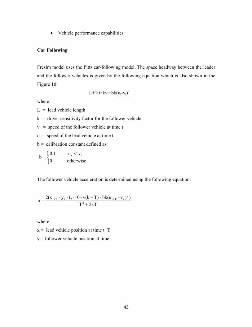
Vehicle performance capabilities •

Car Following

Fresim model uses the Pitts car-following model. The space headway between the leader

and the follower vehicles is given by the following equation which is also shown in the

Figure 10:

L+10+kvt+bk(ut-vt)2

where:

L = lead vehicle length

k = driver sensitivity factor for the follower vehicle

vt = speed of the follower vehicle at time t

ut = speed of the lead vehicle at time t

b = calibration constant defined as:

b 0.1 u v0 otherwise

t t=<

The follower vehicle acceleration is determined using the following equation:

2kTT))v-bk(u - T)+v(k-10-L-y-2(x = a 2

2tT+ttT+t

+

where:

x = lead vehicle position at time t+T

y = follower vehicle position at time t

43

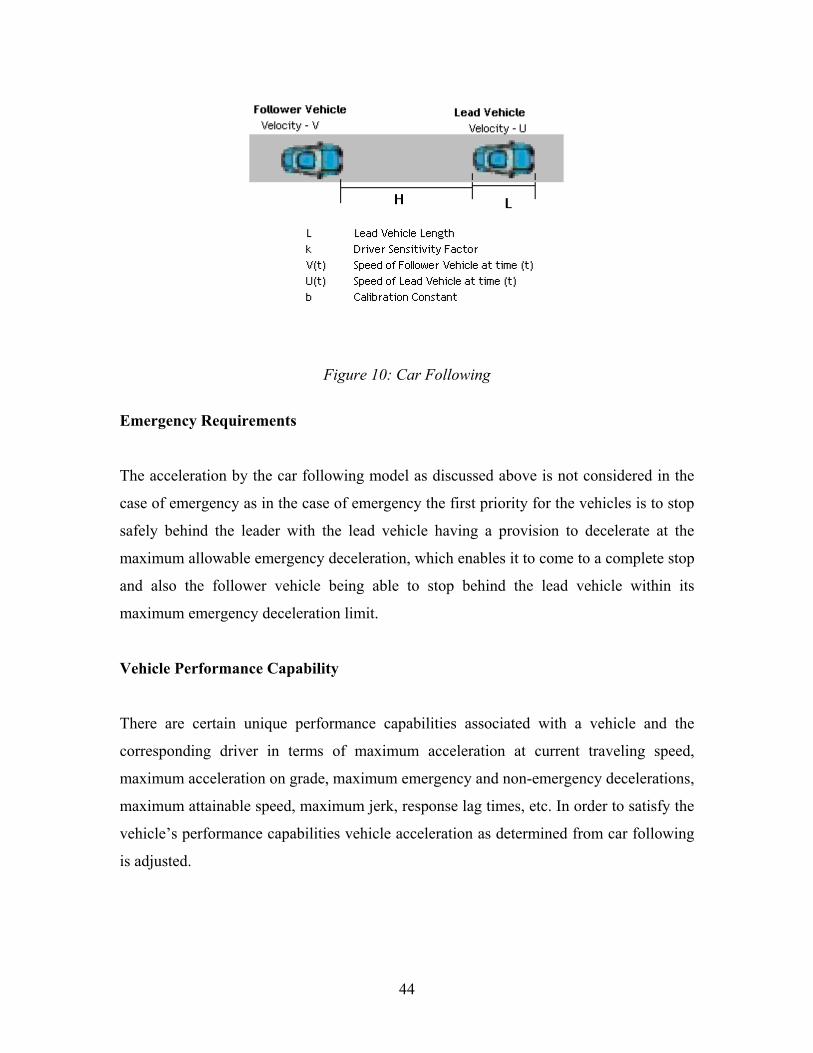
Figure 10: Car Following

Emergency Requirements

The acceleration by the car following model as discussed above is not considered in the

case of emergency as in the case of emergency the first priority for the vehicles is to stop

safely behind the leader with the lead vehicle having a provision to decelerate at the

maximum allowable emergency deceleration, which enables it to come to a complete stop

and also the follower vehicle being able to stop behind the lead vehicle within its

maximum emergency deceleration limit.

Vehicle Performance Capability

There are certain unique performance capabilities associated with a vehicle and the

corresponding driver in terms of maximum acceleration at current traveling speed,

maximum acceleration on grade, maximum emergency and non-emergency decelerations,

maximum attainable speed, maximum jerk, response lag times, etc. In order to satisfy the

vehicle’s performance capabilities vehicle acceleration as determined from car following

is adjusted.

44

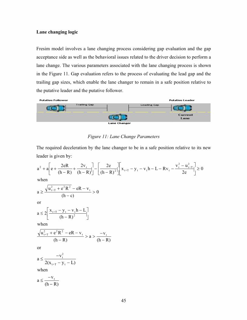
Lane changing logic

Fresim model involves a lane changing process considering gap evaluation and the gap

acceptance side as well as the behavioral issues related to the driver decision to perform a

lane change. The various parameters associated with the lane changing process is shown

in the Figure 11. Gap evaluation refers to the process of evaluating the lead gap and the

trailing gap sizes, which enable the lane changer to remain in a safe position relative to

the putative leader and the putative follower.

Figure 11: Lane Change Parameters

The required deceleration by the lane changer to be in a safe position relative to its new

leader is given by:

a a e 2eR(h R)

2v(h R)

2e(h R)

x y v h L Rvv u

2e0

when

au e R eR v

(h c)0

or

a 2x y v h L

(h R)when

u e R eR v(h R)

av

(h R)

2 t2 t+T t t t

t2

t+T2

t +T2 2 2

t

t +T t t2

t+T2 2 2

t t

+ +−

+−

−

−

− − − − −

−

≥

≥+ − −

−>

≤− − −

−

+ − −−

> >−−

or

av

2(x y L)when

av

(h R)

t2

t+T t

t

≤−− −

≤−−

45

where:

L = length of the putative leader

h = lane changing period

R = driver response lag time

e = maximum emergency deceleration rate

xt+T = position of the putative leader at time t+T

yt = position of the lane changer at time t

vt = speed of the lane changer at time t

ut+T = speed of the putative leader at time t+T

a = lane changer acceleration to remain in safe position

Gap acceptance refers to the process of determining whether the lead and trailing gaps are

acceptable to the lane changer and putative follower. The required deceleration should

not exceed the acceptable level of risk by the lane changer for the lead gap to be

acceptable and similarly the trailing gap becomes acceptable if the required deceleration

for the putative follower does not exceed its acceptable risk. The acceptable levels of risk

for both the lane changer vehicle and the putative follower is manifested as the maximum

acceptable deceleration in performing the lane change. (Halati et al, 1997)

Types of lane changing

Three distinct types of lane changing is recognized in the Fresim model which are as

follows:

Mandatory •

•

•

Discretionary

Anticipatory

Mandatory lane change

Lane Changing is considered mandatory in the situations when traffic is merging from

the on-ramp, when traffic is trying to reach the proper lane to exit the freeway, when

46

vacating a lane blocked by an incident and also when vacating a lane which is dropped

further downstream.

For the driver to perform a lane change, to get out of the auxiliary lane and merge with

the mainline traffic, the acceptable level of risk is obtained as follows:

a a (e a )dll min min= + − [2-29]

where:

al = acceptable deceleration rate

amin = minimum acceptable deceleration

e = emergency deceleration rate

d = distance between the vehicle and the on-ramp gore

l = length of the acceleration auxiliary lane

The acceptable deceleration for a vehicle considering exiting the freeway and trying to

get off ramp is shown as follows:

ae d 200

a (e a )dl

d 200lmin min

=

>

+ − ≤

[2-30]

where:

d = distance between the vehicle and the upstream off-ramp warning sign

l = distance between the off-ramp and its advanced warning sign

Discretionary lane change

It refers to lane changes performed to bypass other slow moving vehicles, to obtain a

more favorable position, and to attain a higher speed. The discretionary lane change logic

involves three behavioral factors on the part of the driver namely motivation, advantage

and urgency.

47

Motivation refers to the desire for performing the discretionary lane change, which is a

function of vehicles present speed and driver’s characteristics. Each vehicle is assigned

an “intolerable“ speed below which the driver is highly motivated to perform the lane

change.

Advantage refers to the benefits gained by performing the lane change and is modeled in

terms of the disadvantage of remaining in the current lane and the gain in moving to a

new lane. The putative factor which represents the perceived gain in performing a lane

change is computed for both lanes adjacent to the current lane. The lane with the largest

putative factor is selected as the target lane.

Urgency in making the lane change refers to the strength of the desire for the lane

change. It is based on the assumption that the driver who is motivated to perform a lane

change but is unable to do so would gradually become impatient and accept higher levels

of risk in performing the lane change.

Anticipatory lane change

It refers to the lane changes performed upstream of the on-ramps in anticipation of

potential slowdown caused by traffic entering the freeway and merging with the mainline

traffic. According to the field observations many a time vehicles on the freeway vacate

the lane when they encounter an on ramp merging. To incorporate this feature in the

model anticipatory lane changing logic was adopted. There are basically two differences

between the anticipatory and discretionary lane change logic in the Fresim model. Firstly

the advantage in performing the lane change is based on the volume and prevailing

average speed in the vicinity of the on-ramp gore and secondly the desire to perform the

lane change, as characterized by the impatience factor, is always set to 1 indicating a high

level of desire.

48

2.6.2.2 NETSIM Model The vehicle movement logic explaining the lateral and longitudinal movements of the

vehicles at the intersections, both signal controlled and sign controlled (both stop and

yield signs) are discussed in detail in the following sections.

Vehicle Movement Logic

Netsim model deals with the movement of traffic on the surface street portion of the

transportation network. Vehicle status in each processing time step is classified as either a

lead, follower, or independent. The vehicle is identified as independent when it is outside

the car-following influence zone as determined by:

s v / 8 v 4ors > 2u + v + 4 and v > u

2≥ + + [2-31]

where:

s = front bumper to rear bumper separation distance

v = follower vehicle speed

u = lead vehicle speed

For free flow conditions the lead and the independent vehicles attempt to attain their

desired free-flow speed subject to their performance capability restrictions. The lead

vehicle in an approach lane which is within the influence zone of the intersection traffic

control device (sign or signal) will begin to decelerate in anticipation of stopping at the

approach stop bar.

Car-Following

The car following logic in CORSIM follows a behavior which deals with avoiding

collision between the vehicles. A collision is considered unavoidable if:

49

s vd2

f< − [2-32]

where:

df = the maximum emergency deceleration of the follower vehicle (default value is 12

ft/sec2)

If collision between the follower and the leader is unavoidable, the vehicle will be

stopped at the rear bumper of the lead vehicle and is given a deceleration of -15 ft/sec2.

When collision is avoidable, the follower vehicle will car-follow it’s leader and the

vehicle’s acceleration is framed from a set of equations.

Gap Acceptance and Gap Evaluation

Gap acceptance model is used in Netsim at sign controlled, both stop and yield signs, and

at signalized intersections for right and permissive left-turning vehicles. The model

compares the available gap in the opposing traffic to the acceptable gap to determine if

the vehicle can be discharged. Available gap in the opposing traffic is evaluated only for

the through moving vehicles (turning vehicles are assumed not to impede each other

movement) and is measured for the first vehicle in each lane of the opposing traffic

stream, unless the first vehicle can clear the intersection prior to the arrival of the turning

vehicle in which case it is measured with respect to the second vehicle. If the opposing

vehicle is in a queue state, the available gap is computed as the remaining time of the

vehicle’s queue discharge headway otherwise the available gap (G) is computed as shown

in the Figure 12. (Halati et al, 1997)

50

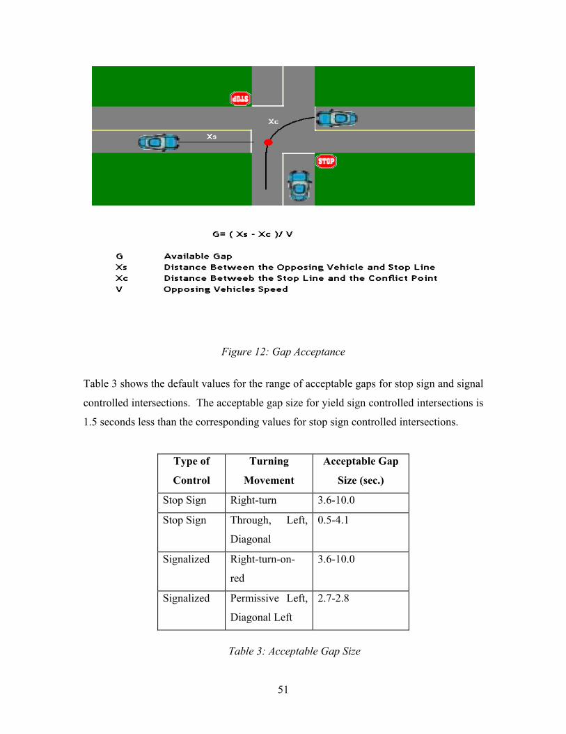
Figure 12: Gap Acceptance

Table 3 shows the default values for the range of acceptable gaps for stop sign and signal

controlled intersections. The acceptable gap size for yield sign controlled intersections is

1.5 seconds less than the corresponding values for stop sign controlled intersections.

Type of

Control

Turning

Movement

Acceptable Gap

Size (sec.)

Stop Sign Right-turn 3.6-10.0

Stop Sign Through, Left,

Diagonal

0.5-4.1

Signalized Right-turn-on-

red

3.6-10.0

Signalized Permissive Left,

Diagonal Left

2.7-2.8

Table 3: Acceptable Gap Size

51

Lane Changing

The Netsim model identifies two types of lane changes as follows:

Mandatory •

• Discretionary

The idea of the lane changing logic is same for this model as the FRESIM model except

for the fact that they do not have anticipatory lane changing environment here. (Halati et

al, 1997)

2.6.3 VISSIM VISSIM is a microscopic, time step and behavior based simulation model developed to

model urban traffic and public transit operations. The program can analyze traffic and

transit operations under constraints such as configuration, traffic composition, traffic

signals, transit stops etc, thus making it a useful tool for the evaluation of various

alternatives based on transportation engineering.

The model consists of two primary components: (1) simulator and (2) signal state

generator (SSG). The simulator generates traffic and is where the user graphically builds

the network. Although links are used in the simulator, VISSIM does not have a traditional

node structure. The lack of nodes provides the user with the flexibility to control traffic

operations (e.g., yield conditions) and vehicle paths within an intersection or interchange.

The simulation system consists of two separate programs. The first program is the traffic

flow model (the kernel of VISSIM), second the signal control model. VISSIM is the

master program, which sends second by second detector values to the signal control

program (slave). The quality of the traffic flow model properties are a major concern as

the traffic flow model used by VISSIM is a discrete, stochastic, time step based (1s)

microscopic model, with driver-vehicle-units (DVU) as single entities. The quality of a

traffic simulation system depends highly on the quality of the traffic flow model at its

52

core. The car-following and the lane-changing model are part of this kernel. (VISSIM

user manual, 2000)

2.6.3.1 Car Following Logic VISSIM uses a psychophysical car following model for longitudinal vehicle movement,

and a rule-based algorithm for lateral movements (lane changing). The basic concept of

this model is that the driver of a faster moving vehicle starts to decelerate as he reaches

his individual perception threshold to a slower moving vehicle. Since he cannot exactly

determine the speed of that vehicle, his speed will fall below that vehicle’s speed until he

starts to slightly accelerate again after reaching another perception threshold. This results

in an iterative process of acceleration and deceleration.

VISSIM simulates traffic flow by moving “driver- vehicle- units” through a network.

Every driver with his specific behavior characteristics is assigned to a specific vehicle. As

a consequence, the driver behavior corresponds to the technical capabilities of his

vehicle. Attributes characterizing each driver - vehicle - unit can be discriminated into

three categories:

1. Technical specifications of the vehicle

Length •

•

•

•

•

•

•

•

•

Maximum speed

Potential acceleration

Actual position within the network

Actual speed and acceleration

2. Behavior of driver- vehicle- unit

Psychophysical sensitivity thresholds of the driver (ability to estimate,

aggressiveness)

Memory of driver

Acceleration based on current speed and driver’s desired speed

3. Interdependence of driver- vehicle- units

Reference to leading and following vehicles on own and adjacent travel lanes

53

Reference to current link and next intersection •

•

•

•

•

•

Reference to next traffic signal

The basic idea of the Wiedemann model is the assumption that a driver can be in one of

four driving modes:

Free driving – In this mode, for a vehicle, there is no influence of preceding

vehicles. The driver tries to maintain his individually desired speed.

Approaching - In this mode, the driver adapts a speed as that of lower speed of

the preceding vehicle. The driver while approaching decelerates so that the

speed difference is zero in the moment he reaches his desired safety distance.

Following – In this kind of mode the driver follows the preceding car without

any conscious acceleration or deceleration. He keeps the safety distance more

or less constant, but again due to imperfect throttle control and imperfect

estimation the speed difference oscillates around zero.

Braking – This refers to an application of medium to high deceleration rates if

the distance falls below the desired safety distance. This can happen if the

preceding car changes speed abruptly, or if a third car changes lanes in front of

the observed driver. (VISSIM User Manual, 2000).

For each mode, the acceleration is described as a result of speed, speed difference,

distance and the individual characteristics of driver and vehicle. The driver switches from

one mode to another as soon as he reaches a certain threshold that can be expressed as a

combination of speed difference and distance. The ability to perceive speed differences

and to estimate distances varies among the driver population, as well as the desired

speeds and safety distances. Because of the combination of psychological aspects and

physiological restrictions of the driver’s perception, the model is called a psychophysical

car-following model.

Vehicles follow each other in an oscillating process. As a faster vehicle approaches a

slower vehicle on a single lane it has to decelerate. The action point of conscious reaction

depends on the speed difference, distance and driver depended behaviour. Figure 13

indicates the oscillating process of this approach. The thresholds of Figure 13 are

54

explained in an abbreviated form. Driver specific perception abilities and individual risk

behaviour is modelled by adding random values to each of the parameters as shown for

AX

Figure 13: Car Following Logic ( Source VISSIM User Manual, 2000).

AX : Desired distance between the fronts of two successive vehicles in a standing queue.

AX = VehL + MinGap + RND1 · AXMult with RND1 normally distributed

N(0.5, 0.15)

ABX : Desired minimum following distance which is a function of AX, a safety delta

distance BX and the speed

ABX := AX + BX · v

SDV: Action point where a driver consciously observes that he approaches a slower car

in front. SDV increases with increasing speed differences ( v∆ ).

55

OPDV: Action point where the following driver notices that he is slower than the leading

vehicle and starts to accelerate again. The variation of OPDV is large.

SDX: Perception threshold to model the maximum following distance which is about

1.5 - 2.5 times ABX.

A following driver reacts to a leading vehicle on up to a certain distance, which is about

150 m. The minimum acceleration and deceleration rate is set to be 0.2 m/s². Maximum

rates of acceleration depend on technical features of vehicles, which are usually lower for

trucks than the personal desire of its driver. The model includes a rule for exceeding the

maximum deceleration rate in case of emergency. This happens if ABX is exceeded. The

values of the thresholds depend on the present speed of the vehicle. (VISSIM User

Manual, 2000)

2.6.3.2 Lane Changing Logic

On multi-lane links vehicles check whether they improve by changing lanes and if so,

they check the possibility of finding acceptable gaps on neighboring lanes. Thus a

hierarchical set of rules is formulated to model lane changes. A driver has a desire to

change lane if he has to drive slower than his desired speed due to a slow leading vehicle

or in case of an upcoming junction with a special turning lane. Then the driver checks

whether he improves his present situation by changing lanes. Last he checks whether he

can change without generating a dangerous situation. In case of multi-lane approaches

towards intersections this method will lead to evenly used lanes unless routing

information forces vehicles to keep lanes.

The basis for lane changing logic is to define time-distance relationships and times of

start and end of lane changing maneuvers. The combination of both data types is allowed

to determine speeds and distances between vehicles.

There are two types of lane changing in VISSIM

• Changes to faster lane

56

Further the changes to faster lane can be classifies as

• FREE lane changes

• LEAD lane changes

• LAG lane changes

• GAP lane changes

• Changes to slower lane

These are further classified as

• FREE lane changes

• ACCEL lane changes

2.6.4 INTEGRATION The INTEGRATION model is a trip-based microscopic traffic simulation model. It is a

continuous model, which is based on speed and distance variables. The model is designed

to trace both the lateral and longitudinal movements of an individual vehicle from a

vehicle’s origin to its destination at a level of resolution of one status update every 1/10th

of a second, or deci-second. INTEGRATION uses a steady state car following model

proposed by Van Aerde that combines the Pipes and Greenshields models into a single

regime model, which is a four-parameter model.

2.6.4.1 Vehicle Movement Logic The vehicle movement logic deals with a discussion on how the model has been designed

to estimate the steady-state speeds of vehicles that are driving at constant speeds within

different traffic conditions. This discussion emphasizes the relationship between the

macroscopic fundamental diagrams for the traffic flow of groups of vehicles, to the

microscopic car-following logic of individual vehicles. Macroscopic traffic flow theory

describes the flow rate, speed, density of the traffic flow and the rate of propagation of

any queues that form when the traffic demand exceeds the available capacity.

Microscopic traffic flow theory deals with the speeds and headways which individual

57

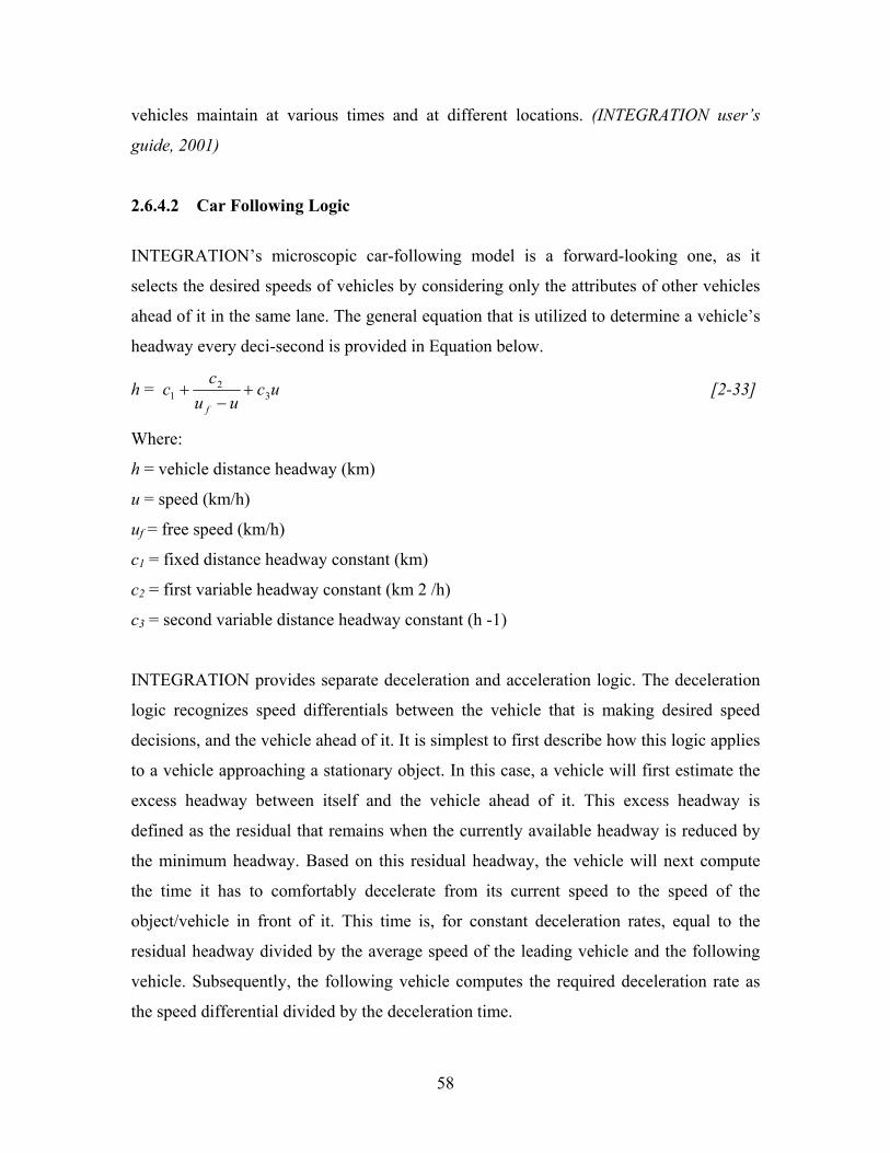
vehicles maintain at various times and at different locations. (INTEGRATION user’s

guide, 2001)

2.6.4.2 Car Following Logic

INTEGRATION’s microscopic car-following model is a forward-looking one, as it

selects the desired speeds of vehicles by considering only the attributes of other vehicles

ahead of it in the same lane. The general equation that is utilized to determine a vehicle’s

headway every deci-second is provided in Equation below.

h = ucuu

c

f3

21 +

−+c [2-33]

Where:

h = vehicle distance headway (km)

u = speed (km/h)

uf = free speed (km/h)

c1 = fixed distance headway constant (km)

c2 = first variable headway constant (km 2 /h)

c3 = second variable distance headway constant (h -1)

INTEGRATION provides separate deceleration and acceleration logic. The deceleration

logic recognizes speed differentials between the vehicle that is making desired speed

decisions, and the vehicle ahead of it. It is simplest to first describe how this logic applies

to a vehicle approaching a stationary object. In this case, a vehicle will first estimate the

excess headway between itself and the vehicle ahead of it. This excess headway is

defined as the residual that remains when the currently available headway is reduced by

the minimum headway. Based on this residual headway, the vehicle will next compute

the time it has to comfortably decelerate from its current speed to the speed of the

object/vehicle in front of it. This time is, for constant deceleration rates, equal to the

residual headway divided by the average speed of the leading vehicle and the following

vehicle. Subsequently, the following vehicle computes the required deceleration rate as

the speed differential divided by the deceleration time.

58

The following vehicle will select a constant deceleration rate that allows it to just come to

a stop at jam density headway behind a following vehicle. If the leading vehicle is

actually moving, the following vehicle would attempt to decelerate at a constant rate in

such a manner as to attain the speed of the leading vehicle when it reached the location

that is single jam density headway behind its current location. By the time the following

vehicle would reach this location, the lead vehicle would already have moved ahead on

the highway, resulting in an asymptotic deceleration of the follower vehicle to the lead

vehicle’s speed, rather than a constant deceleration. Similarly, if the lead vehicle were

accelerating, the follower vehicle would only continue to decelerate until it was traveling

at the same speed as the lead vehicle. From that point onwards, the follower vehicle

would likely begin to accelerate again, as the increasing gap to the lead vehicle would

cause the follower vehicle to perceive increasing desired speeds.

While deceleration is governed primarily by kinematics, the acceleration rate of vehicles

is governed by dynamics. Specifically, a vehicle with a desired speed that is greater than

its current speed will attempt to accelerate at the maximum possible rate. This maximum

possible rate can be constrained using one of two different mechanisms. Within the first

mechanism, the maximum acceleration rate of a vehicle is set to be linearly dependent

upon the vehicle’s current speed. This results in vehicles being able to achieve higher

acceleration rates at lower speeds, and lower acceleration rates at high speeds.

(“Microsimulation of Traffic with and without Adaptive Cruise Control: Model Logic”,

Paper submitted to ITS America).

2.6.4.3 Lane Changing Logic Two distinct types of lane changing is recognized in the INTEGRATION which are as

follows:

Mandatory •

• Discretionary

When a vehicle travels down a particular link, it may make discretionary lane changes,

mandatory lane changes, or both. Discretionary lane changes are a function of the

59

prevailing traffic conditions, while mandatory lane changes are usually a function of the

prevailing network geometry.

In order to determine if a discretionary lane change should be made, each vehicle computes

three speed alternatives each deci-second. The first alternative represents the potential speed

at which the vehicle could continue to travel in its current lane, while the second and third

choices represent the potential speeds that this vehicle could travel in the lanes immediately

to the left and to the right of its current lane. These speed comparisons are made on the basis

of the available headway in each lane, and pre-specified biases for the vehicle to remain in

the lane in which it is already traveling or to move to the shoulder lane. A vehicle will then

elect to try to change into that lane which will permit it to travel at the highest of these three

potential speeds.

While discretionary lane changes are made by vehicles in order to maximize their speed,

mandatory lane changes arise primarily from a need for vehicles to maintain lane

connectivity at the end of each link. The lane connectivity requires that eventually every

vehicle must be in one of the lanes that are directly connected to the relevant downstream

link onto which the vehicle anticipates turning. A unique feature of INTEGRATION’s lane

changing model is that the lane connectivity at any diverge or merge is computed internally.

Once a lane-changing maneuver has been initiated, a subsequent lane change is not permitted

until a pre-specified minimum amount of time has elapsed. In the first instance, this

minimum interval ensures that lane changes usually involve a finite length of time to

materialize, and that two consecutive lane changes cannot be executed one immediately after

the other. Furthermore, while an actual lane-changing maneuver is in progress, the vehicle is

modeled as if it partially restricts the headway in both the lane it is moving from and the lane

it is changing into. This concurrent presence in two lanes will result in an effective capacity

reduction. (INTEGRATION User’s Guide, 2001).

60

2.6.4.4 Vehicle Movements at Intersections

The main roadway element within most urban areas is the presence of signalized

intersections. Within INTEGRATION, a signalized link is identical in virtually all

respects to a freeway link. When the traffic light is red, vehicles must still obey the link’s

car-following logic, except that a red traffic signal is now considered as an additional

vehicle positioned just beyond the stop line at the end of each lane on the link. This

virtual vehicle creates a reduction in the vehicle’s perceived headway, and causes

vehicles that approach a red signal to slow down as their headway to the traffic signal

decreases. Eventually, the first vehicle to approach the red signal comes to a complete

stop upstream of the stop line. Subsequent vehicles then automatically queue upstream of

the first vehicle in a horizontal queue, where the minimum spacing of vehicles in this

horizontal queue is governed by the user-specified jam density.

When the effective green indication commences, the virtual object at the signal stop line

of each lane is removed and the first vehicle in queue faces an uninterrupted headway

down the next downstream link. The initial acceleration of the first vehicle in the queue,

together with the subsequent impact of the model’s car-following logic on any additional

vehicles, causes two shock waves to form concurrently. (INTEGRATION user’s guide,

2001).

2.7 Comparison and Contrast Between TRANSIMS, CORSIM VISSIM and INTEGRATION

The following discussion will compare the TRANSIMS, CORSIM, VISSIM and

INTEGRATION models in more detail.

The models are similar as they are designed to model any combination of surface

street and freeway facilities, including most signal control and other operational

strategies. The models provide detailed and focused output, in tabular format and

via animated graphics. The main differences between the models are in vehicle

and driver behavior, primarily in the car-following and gap acceptance logic.

•

61

VISSIM, CORSIM and INTEGRATION are stochastic microscopic computer

simulation programs while TRANSIMS is a mesoscopic simulation program. All

the models are capable of modeling individual vehicle interactions on complex

roadway networks. The models use inputs such as lane assignments and

geometries, intersection turning movement volumes, vehicle speeds, percentages

of vehicles by type, and pretimed and/or actuated signal timing. And the programs

produce output that contains measures of effectiveness commonly used in the

traffic engineering profession, including total delay, stopped delay, and queue

lengths.

•

•

•

•

VISSIM is more capable of modeling the interaction of various modes of transit

with automobile traffic while CORSIM, INTEGRATION and TRANSIMS can

effectively model simple bus routes within a roadway network. VISSIM and

TRANSIMS can model light rail transit and can model more bus routes and bus

stops than CORSIM and INTEGRATION. In addition, unlike CORSIM,

INTEGRATION and TRANSIMS, VISSIM is capable of modeling gates at rail

crossings as well as complex traffic control strategies such as preemption and

priority systems.

User Interface: CORSIM input files can be quickly created either through ITRAF

or Synchro. In order to take full advantage of CORSIM’s capabilities, it is often

necessary to use a text editor to adjust the input file. The input data files for

INTEGRATION can be generated/modified using any standard editor,

spreadsheet or word processor. The Windows version of INTEGRATION model

provides on-screen graphics that continuously reflect the network status. The

input files in TRANSIMS can be created using any text editor such as vi, gvim,

gnotepad, pico etc. It has the capability of viewing the output using the output

visualizer provided with TRANSIMS in the XWindows. VISSIM network editing

is done completely through the use of its Graphical User Interface, which runs in

various versions of Microsoft Windows. VISSIM can also import scaled versions

of background bitmap files, which can be used to build the model upon.

Network Structure: Unlike CORSIM, INTEGRATION and TRANSIMS, which

use a link-node network structure, VISSIM uses links and connectors. These links

62

and connectors allow VISSIM to be very flexible when working with complex

geometries allowing it to accurately model curvature while CORSIM,

INTEGRATION and TRANSIMS have a tendency to show strange loops or other

graphical misrepresentations based upon limited input options.

Vehicle Entry: CORSIM generates vehicles using a uniform distribution at its

entry points. VISSIM generates vehicles randomly. It follows Poisson arrival

distribution. The movement of vehicles in TRANSIMS follows the distributions

as specified in traveler plans.

•

•

•

•

Mid-Block Source/Sinks: CORSIM Source and Sink nodes add or remove

vehicles from a link without regard to lane position, acceleration, or deceleration.

Specifically, when using source nodes, vehicles just appear on the roadway in any

lane, traveling at full speed. When using sink nodes, vehicles just disappear from

the roadway in any lane, traveling at full speed. This does not accurately represent

the effect of entering and exiting vehicles would have on the link. In contrast,

VISSIM’s flexible link capabilities can be used to create mid-block source and

sink locations where vehicles accelerate, decelerate, and use lanes more

realistically when they enter or exit. In addition, VISSIM can more easily account

for these vehicles in the statistics if desired. In TRANSIMS parking places model

the Source or Sinks on the network. These parking places are placed anywhere on

the links and the vehicles are ejected from the parking places and placed on the

link with a velocity depending on the gap ahead. And in the same way vehicles

are removed from the network and placed in the parking lots without any

deceleration.

Output: CORSIM provides detailed output in a series of standardized tables

contained in one output file. This output is usually easy to read and has been

summarized to a great extent. The output in VISSIM, INTEGRATION and

TRANSIMS is present in separate files. The user or analyst can specify the

amount and the type of data to be collected. An advantage of VISSIM and

TRANSIMS is that they can produce very detailed results on any time interval

Driver Characteristics: CORSIM and VISSIM provide a wide variety of

configurable parameters that model a driver behavior in a traffic stream.

63

TRANSIMS, on the other hand provides very few driver characteristic

configurable parameters. INTEGRATION provides driver characteristics on a

lane-by-lane basis through adjustable flow density relationships.

2.8 Description of the Weaving Sections Weaving is defined as the crossing of two streams traveling in the same direction along a

significant length of the highway without the aid of traffic control devices. Weaving areas

are formed when a merge area is closely followed by a diverge area, or when an on ramp

is closely followed by an off ramp and the two are joined by an auxiliary lane. Weaving

areas require intense lane changing maneuvers, as drivers must access lanes appropriate

to their desired exit point.

As a result, traffic in a weaving area is subject to turbulence in excess of that normally

present on the basic highway sections. The drivers from two upstream lanes compete for

space and merge into a single lane and then diverge into two different upstream lanes

because of which capacity is reduced in these weaving areas. Configuration (number of

entry lanes and exit lanes and relative placement) is one of the important geometric

factors that need to be considered, as lane changing is a complex component of the

weaving areas. Some of the other factors to be considered are speed, level of service,

volume distribution etc. The operational problems and special design requirements are

often presented by the turbulence created by the “weaving” of vehicles. (HCM 2000)

Weaving length

The weaving area length is measured from the merge gore area at a point where the right

edge of the freeway shoulder lane and the left edge of the merging lane(s) are 2 ft apart to

a point at the diverge gore area where the two edges are 12 ft apart. The time and space

are constrained by the length of the weaving area, in which the drivers have to make the

necessary and the required lane changes. The intensity of the lane changing as well as the

turbulence increases as the length of the weaving area decreases, other factors remaining

64

a constant. There is also a reduction in the average speed of the vehicles in the weaving

area (HCM 2000)

Configuration

Configuration of a weaving area refers to the relative placement and the number of entry

lanes and exit lanes for the section. The performance of a weaving section is drastically

affected by this critical geometric characteristic feature. The number of lane changes

required of each weaving movement is an influential factor for the weaving segment

configuration. The primary types of weaving configuration are categorized as Type A,

Type B and Type C, according to the Highway Capacity Manual. The types are defined

in terms of the minimum number of lane changes that must be made by weaving vehicles

as they traverse the section. (HCM 2000)

Type A Weaving Areas

According to this type of configuration weaving vehicles in both the directions must

make one lane change to successfully complete a weaving maneuver. The two types of

weaving areas for Type A configuration are shown in Figure 14. An on-ramp followed by

an off-ramp, with a continuous auxiliary lane between the ramps, is shown in Figure 14a.

In this configuration one lane change needs to be performed by all on ramp vehicles out

of the auxiliary lane into the shoulder lane of the freeway, and all off-ramp vehicles must

make a lane change from the shoulder lane of the freeway to the auxiliary lane.

( a ) ( b )

Figure 14 a & b: Type A Weaving Sections (Source HCM)

65

Ramp-weave sections are those that are formed by on-ramp/off-ramp sequences joined by

continuous auxiliary lanes. A major weaving section characterized by three or more entry

and exit roadways having multiple lanes is shown in the Figure 14(b). To get into the

desired lanes all weaving vehicles in this type of configuration need to make at least one

lane change. The crown line (the line connecting the nose of the entrance gore area to the

nose of the exit gore area) is a characteristic feature of this type of weaving configuration.

This crown line is crossed over by every weaving vehicle that makes a lane change. The

impact of ramp geometrics on speed, the ramp weave model having its vehicle to

accelerate or decelerate as they move from the on to the off-ramp is identified as the

primary difference between the two types of movements as shown in the Figure 14. The

weaving vehicles are usually confined to the two lanes adjacent to the crown line in the

weaving section as they cross the crown lane in this type of configuration. A significant

effect of this configuration on operations is the maximum number of lanes that weaving

vehicles occupy while traversing the section. (HCM 2000)

Type B Weaving Areas

In this type of configuration weaving vehicles in one direction may complete a weaving

maneuver without making a lane change, whereas other vehicles in the weaving segment

must make one lane change to successfully complete a weaving maneuver. Three

different types of Type B configurations are shown in Figure 15 a, b and c. A lane change

is not required by the movement B-C while one lane change is required for A-D. This is

achieved by lane balancing as shown in Figure 15(a), while in b this is achieved by a lane

in Leg A merging with a lane from leg B at the entrance gore area.

66

( a ) ( b )

( c )

A

B

C

D

Figure 15: Type B Weaving Sections (Source HCM)

This kind of a weaving configuration is found to be more efficient in carrying large

weaving volumes much attributed to the provision of a through lane from one weaving

movement. The weaving vehicles are allowed to occupy a substantial number of lanes in

the weaving section for this type of configuration and not restricted as in Type A

configuration sections. (HCM 2000)

Type C Weaving Areas

In this weaving vehicles in one direction may complete a weaving maneuver without

making a lane change, whereas other vehicles in the weaving segment must make two or

more lane changes to successfully complete a weaving maneuver. The weaving areas in

Type C configuration are very similar to those of Type B. The difference crops up in the

number of lane changes necessary for the other weaving movement. Figure 16 shows

different types of movements for this type of configuration. A lane change is not required

for the movement B-C while the movement A-D requires two lane changes.

67

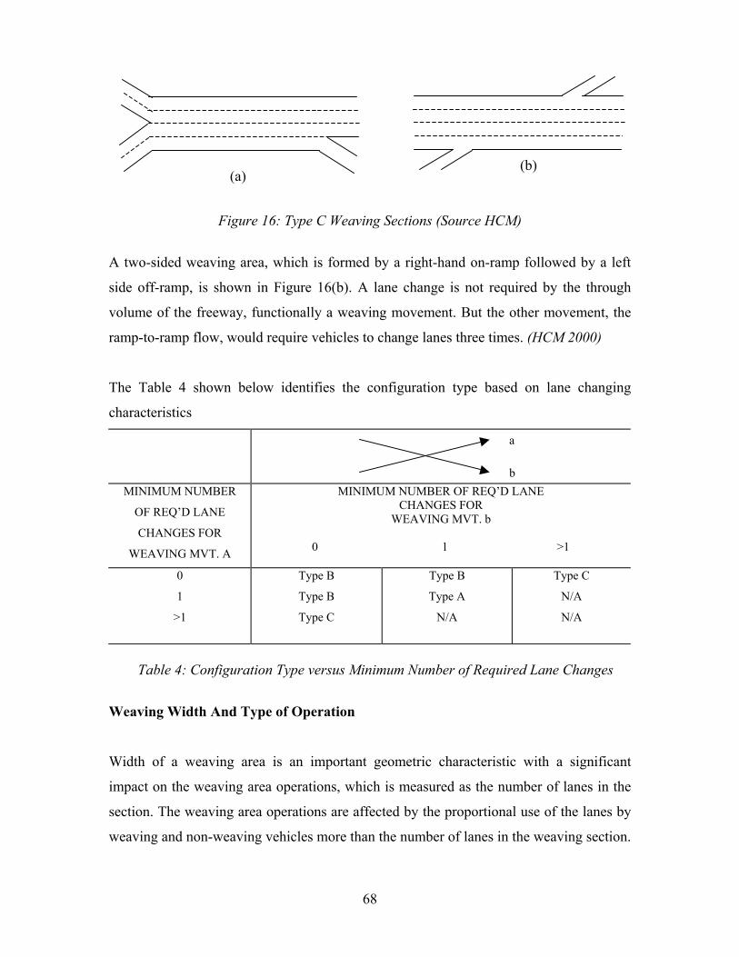
(a) (b)

Figure 16: Type C Weaving Sections (Source HCM)

A two-sided weaving area, which is formed by a right-hand on-ramp followed by a left

side off-ramp, is shown in Figure 16(b). A lane change is not required by the through

volume of the freeway, functionally a weaving movement. But the other movement, the

ramp-to-ramp flow, would require vehicles to change lanes three times. (HCM 2000)

The Table 4 shown below identifies the configuration type based on lane changing

characteristics

MINIMUM NUMBER

OF REQ’D LANE

CHANGES FOR

WEAVING MVT. A

MINIMUM NUMBER OF REQ’D LANE CHANGES FOR

WEAVING MVT. b 0 1 >1

0

1

>1

Type B

Type B

Type C

Type B

Type A

N/A

Type C

N/A

N/A

a

b

Table 4: Configuration Type versus Minimum Number of Required Lane Changes

Weaving Width And Type of Operation

Width of a weaving area is an important geometric characteristic with a significant

impact on the weaving area operations, which is measured as the number of lanes in the

section. The weaving area operations are affected by the proportional use of the lanes by

weaving and non-weaving vehicles more than the number of lanes in the weaving section.

68

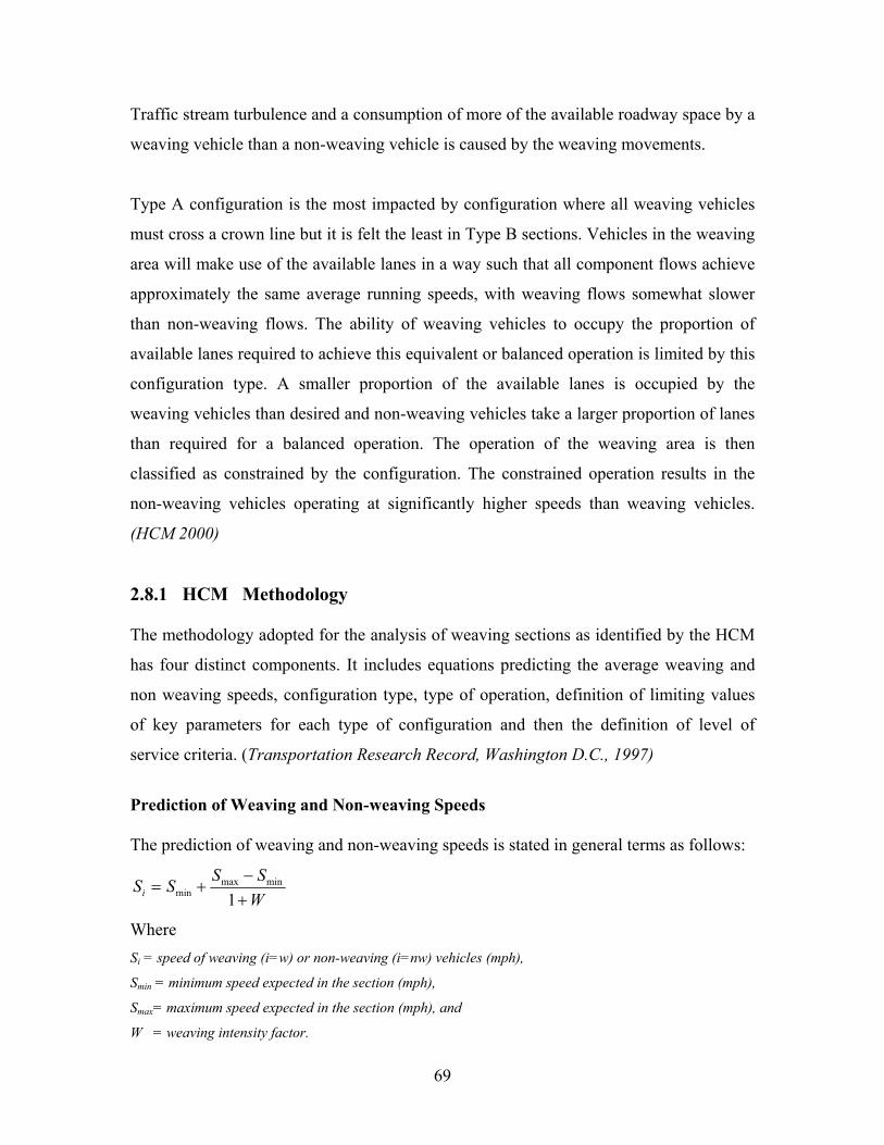
Traffic stream turbulence and a consumption of more of the available roadway space by a

weaving vehicle than a non-weaving vehicle is caused by the weaving movements.

Type A configuration is the most impacted by configuration where all weaving vehicles

must cross a crown line but it is felt the least in Type B sections. Vehicles in the weaving

area will make use of the available lanes in a way such that all component flows achieve

approximately the same average running speeds, with weaving flows somewhat slower

than non-weaving flows. The ability of weaving vehicles to occupy the proportion of

available lanes required to achieve this equivalent or balanced operation is limited by this

configuration type. A smaller proportion of the available lanes is occupied by the

weaving vehicles than desired and non-weaving vehicles take a larger proportion of lanes

than required for a balanced operation. The operation of the weaving area is then

classified as constrained by the configuration. The constrained operation results in the

non-weaving vehicles operating at significantly higher speeds than weaving vehicles.

(HCM 2000)

2.8.1 HCM Methodology The methodology adopted for the analysis of weaving sections as identified by the HCM

has four distinct components. It includes equations predicting the average weaving and

non weaving speeds, configuration type, type of operation, definition of limiting values

of key parameters for each type of configuration and then the definition of level of

service criteria. (Transportation Research Record, Washington D.C., 1997)

Prediction of Weaving and Non-weaving Speeds

The prediction of weaving and non-weaving speeds is stated in general terms as follows:

WSSSSi +

−+=

1minmax

min

Where Si = speed of weaving (i=w) or non-weaving (i=nw) vehicles (mph),

Smin = minimum speed expected in the section (mph),

Smax= maximum speed expected in the section (mph), and

W = weaving intensity factor.

69

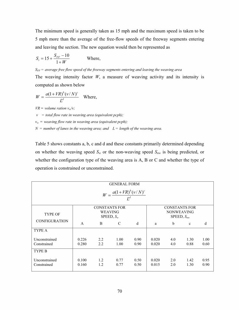
The minimum speed is generally taken as 15 mph and the maximum speed is taken to be

5 mph more than the average of the free-flow speeds of the freeway segments entering

and leaving the section. The new equation would then be represented as

WSS FF

i +−

+=1

1015 Where,

SFF = average free flow speed of the freeway segments entering and leaving the weaving area The weaving intensity factor W, a measure of weaving activity and its intensity is

computed as shown below

d

cb

LNvVRaW )/()1( +

= Where,

VR = volume ration vw/v;

v = total flow rate in weaving area (equivalent pcph);

vw = weaving flow rate in weaving area (equivalent pcph);

N = number of lanes in the weaving area; and L = length of the weaving area.

Table 5 shows constants a, b, c and d and these constants primarily determined depending

on whether the weaving speed Sw or the non-weaving speed Snw is being predicted, or

whether the configuration type of the weaving area is A, B or C and whether the type of

operation is constrained or unconstrained.

GENERAL FORM

d

cb

LNvVRaW )/()1( +

=

CONSTANTS FOR WEAVING SPEED, Sw

CONSTANTS FOR NONWEAVING

SPEED, Snw

TYPE OF

CONFIGURATION A B C d a b c d

TYPE A Unconstrained Constrained

0.226 0.280

2.2 2.2

1.00 1.00

0.90 0.90

0.020 0.020

4.0 4.0

1.30 0.88

1.00 0.60

TYPE B Unconstrained Constrained

0.100 0.160

1.2 1.2

0.77 0.77

0.50 0.50

0.020 0.015

2.0 2.0

1.42 1.30

0.95 0.90

70

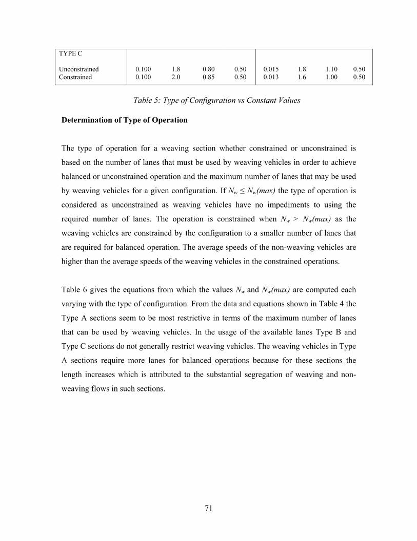
TYPE C Unconstrained Constrained

0.100 0.100

1.8 2.0

0.80 0.85

0.50 0.50

0.015 0.013

1.8 1.6

1.10 1.00

0.50 0.50

Table 5: Type of Configuration vs Constant Values

Determination of Type of Operation

The type of operation for a weaving section whether constrained or unconstrained is

based on the number of lanes that must be used by weaving vehicles in order to achieve

balanced or unconstrained operation and the maximum number of lanes that may be used

by weaving vehicles for a given configuration. If Nw ≤ Nw(max) the type of operation is

considered as unconstrained as weaving vehicles have no impediments to using the

required number of lanes. The operation is constrained when Nw > Nw(max) as the

weaving vehicles are constrained by the configuration to a smaller number of lanes that

are required for balanced operation. The average speeds of the non-weaving vehicles are

higher than the average speeds of the weaving vehicles in the constrained operations.

Table 6 gives the equations from which the values Nw and Nw(max) are computed each

varying with the type of configuration. From the data and equations shown in Table 4 the

Type A sections seem to be most restrictive in terms of the maximum number of lanes

that can be used by weaving vehicles. In the usage of the available lanes Type B and

Type C sections do not generally restrict weaving vehicles. The weaving vehicles in Type

A sections require more lanes for balanced operations because for these sections the

length increases which is attributed to the substantial segregation of weaving and non-

weaving flows in such sections.

71

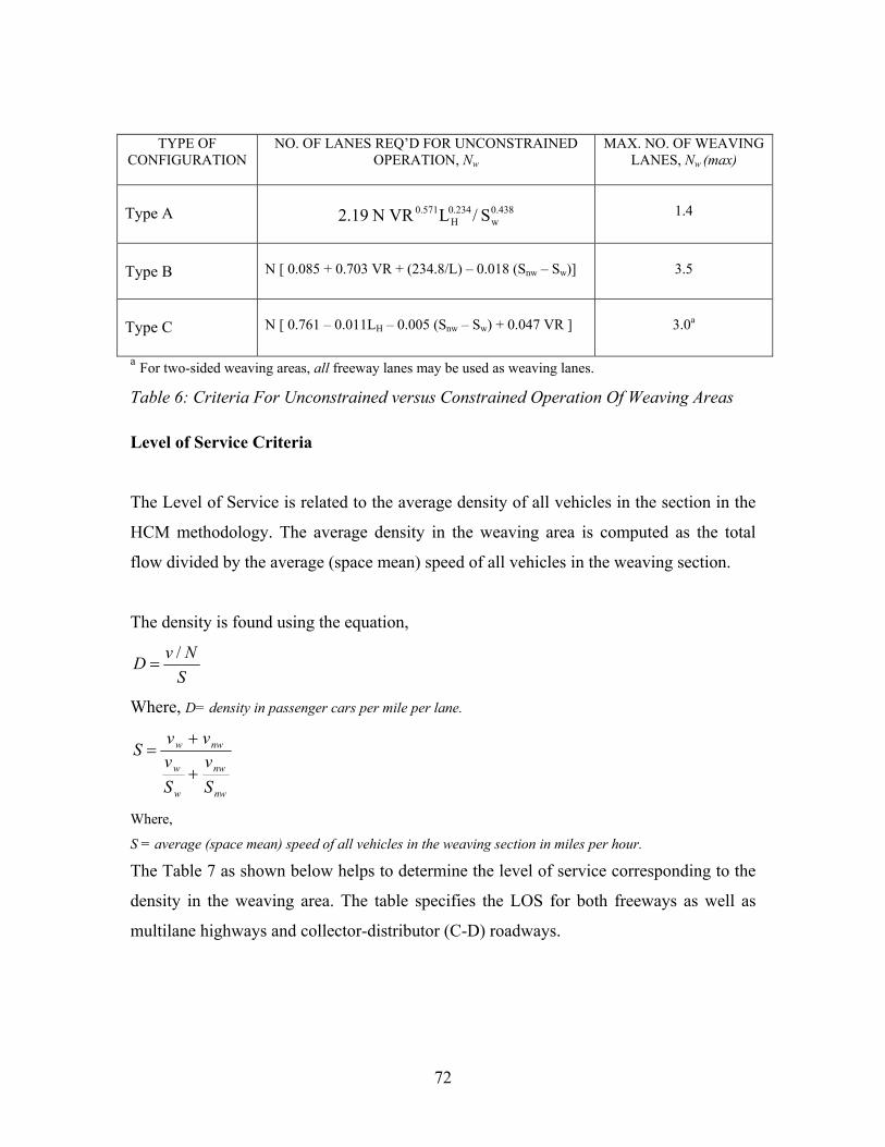
TYPE OF

CONFIGURATION

NO. OF LANES REQ’D FOR UNCONSTRAINED OPERATION, Nw

MAX. NO. OF WEAVING LANES, Nw (max)

Type A

0.438w

0.234H

0.571 S/ LVRN 19.2

1.4

Type B

N [ 0.085 + 0.703 VR + (234.8/L) – 0.018 (Snw – Sw)]

3.5

Type C

N [ 0.761 – 0.011LH – 0.005 (Snw – Sw) + 0.047 VR ]

3.0a

a For two-sided weaving areas, all freeway lanes may be used as weaving lanes.

Table 6: Criteria For Unconstrained versus Constrained Operation Of Weaving Areas

Level of Service Criteria

The Level of Service is related to the average density of all vehicles in the section in the

HCM methodology. The average density in the weaving area is computed as the total

flow divided by the average (space mean) speed of all vehicles in the weaving section.

The density is found using the equation,

SNvD /

=

Where, D= density in passenger cars per mile per lane.

nw

nw

w

w

nww

Sv

Sv

vvS

+

+=

Where,

S = average (space mean) speed of all vehicles in the weaving section in miles per hour.

The Table 7 as shown below helps to determine the level of service corresponding to the

density in the weaving area. The table specifies the LOS for both freeways as well as

multilane highways and collector-distributor (C-D) roadways.

72

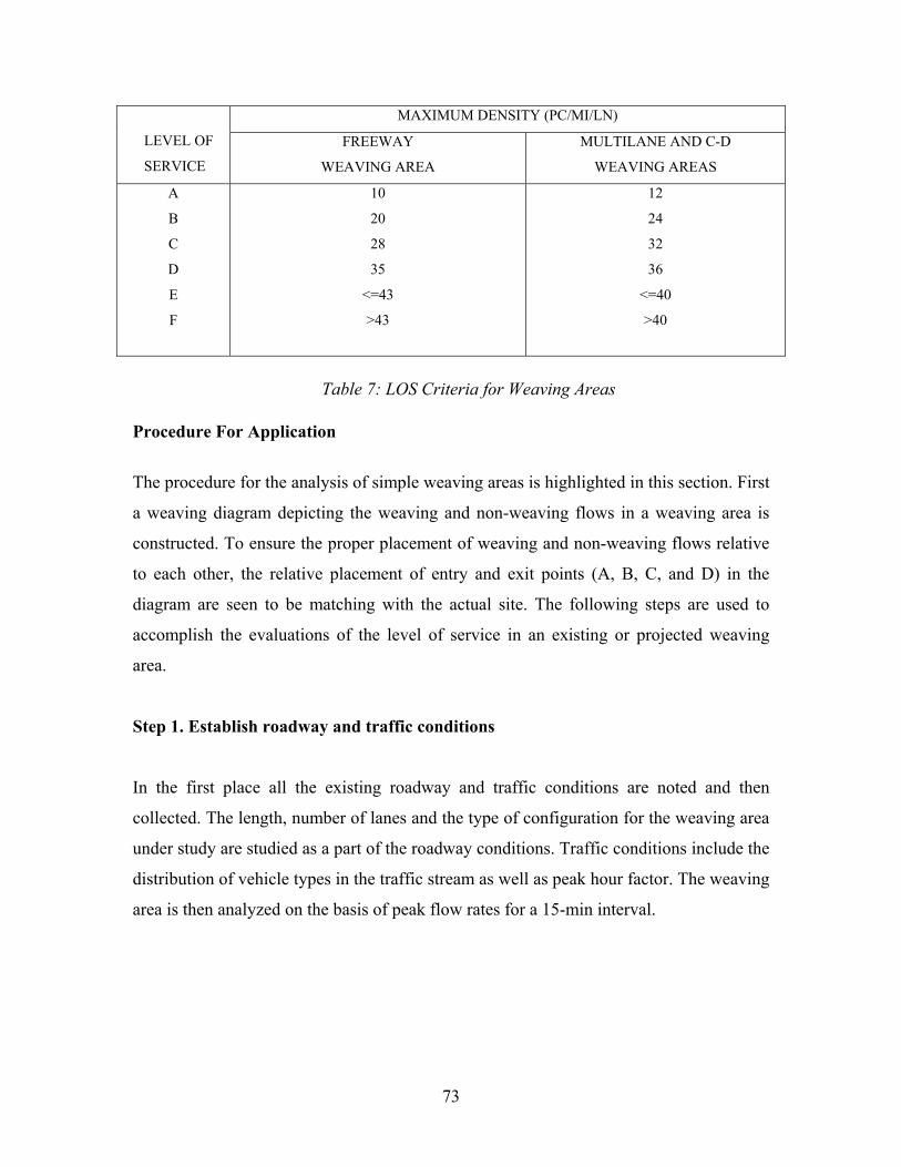
MAXIMUM DENSITY (PC/MI/LN)

LEVEL OF

SERVICE

FREEWAY

WEAVING AREA

MULTILANE AND C-D

WEAVING AREAS

A

B

C

D

E

F

10

20

28

35

<=43

>43

12

24

32

36

<=40

>40

Table 7: LOS Criteria for Weaving Areas

Procedure For Application

The procedure for the analysis of simple weaving areas is highlighted in this section. First

a weaving diagram depicting the weaving and non-weaving flows in a weaving area is

constructed. To ensure the proper placement of weaving and non-weaving flows relative

to each other, the relative placement of entry and exit points (A, B, C, and D) in the

diagram are seen to be matching with the actual site. The following steps are used to

accomplish the evaluations of the level of service in an existing or projected weaving

area.

Step 1. Establish roadway and traffic conditions

In the first place all the existing roadway and traffic conditions are noted and then

collected. The length, number of lanes and the type of configuration for the weaving area

under study are studied as a part of the roadway conditions. Traffic conditions include the

distribution of vehicle types in the traffic stream as well as peak hour factor. The weaving

area is then analyzed on the basis of peak flow rates for a 15-min interval.

73

Step 2. Convert all traffic volumes to peak flow rates

As the speed and lane use algorithms are based on peak flow rates, all component flows

must be converted to flow rate for peak 15 min, by using following equation:

pwHV xfxfPHFxfVv =

Where, v=flow rate for peak 15 min under ideal conditions (pcph);

V=hourly volume under prevailing conditions (veh/hr);

PHF= peak-hour Factor;

fHV=heavy-vehicle adjustment factor;

fp=driver population adjustment factor.

Step 3. Construction of Weaving Diagram

It is necessary and helpful to construct a weaving diagram that shows all flows indicated

at peak flow rates under ideal conditions in passenger cars per hour.

Step 4. Computation of Unconstrained Weaving and Non-weaving Speeds

In this step it is assumed that the operation is unconstrained. The weaving intensity factor

for the appropriate configuration is read from Table 4. The average (space mean) speed is

then computed for the weaving and non-weaving vehicles.

Step 5. Check for Constrained operation

Using the speeds computed in the previous step, an estimate of the number of lanes used

by weaving vehicles to achieve unconstrained operation is made using the equations

specified in the Table 6. This computed value of Nw is then compared with Nw(max)

(read from Table 6). If Nw(max) is less than or equal to Nw then the operation is

constrained as per definition and hence the assumption that this is an unconstrained

operation is accurate. If the condition is not satisfied then the operation is constrained and

74

the values of the weaving and non-weaving speeds are recomputed using the constrained

weaving intensity factor for the appropriate configuration.

Step 6. Computation of Average (Space Mean) Speed and Density in Weaving Area

The equation stated earlier in the methodology is used to compute the average (space

mean) speed of all vehicles in the weaving section. Then this average speed (space mean)

is used in the equation to compute the density of the weaving area.

Step 7. Check for Weaving Area Limitations

As a final check to see if the whole analysis is acceptable the table specifying the

limitations on the weaving sections is consulted and is made sure that none of the

parameters have exceeded their limits specified by the table.

Step 8. Determination of Level of Service

The estimated value of density, D, in the weaving area is compared with the criteria in the

Table 7 to determine the prevailing Level of Service.

2.9 Past Research Related to Freeway Weaving Analysis

The methodology adopted in the comparative analysis is to model different kinds of

weaving configurations using TRANSIMS, CORSIM, VISSIM and INTEGRATION. To

adjust the simulation model, various factors such as capacity of the weaving section,

driver characteristics, roadway geometrics, parameters influencing the weaving behavior

etc need to be studied. As the scope of the research is to identify various parameters,

which affect the result of simulation and methods to improve them, the next few

paragraphs talk about some earlier research done on some of the various parameters,

which might affect the calibration of the model and their resulting conclusions.

75

A study on capacity and level of service at ramp freeway junctions by Roger P. Roess

and Jose M. Ulerio found that if some parameters such as volume distribution, speed

variance can be improved, its use could augment field data and allow more consistent and

thorough calibration of regression/simulation models. The importance of the driver

population to the freeway traffic operation analysis also should not be neglected. In

analyzing freeway capacity, one of the most important factors is speed because service

flow rate can be obtained from the value of density multiplied by the value of average

speed. Most traditional weaving analysis methods use roadway geometry and traffic

volumes as inputs and provide an estimate of speed as an output. The use of speed for

assessing the capacity and level of service for weaving has proved to be a poor choice.

One reason is that speed is not very sensitive to flow at saturation level. A study

conducted by Halati et al has shown that the concept of a stable relationship between

speed and flow is fundamentally flawed. As flow nears capacity, it begins a series of fast

and unstable jumps from the smooth flow to an unstable one. With this approach, traffic

only flows at capacity speed while transitioning from fast sub capacity flow to a slow

congested flow. In effect, capacity speed is ephemeral and can be quantified in averages.

Since speed has been identified as one of the important factors that might affect the

calibration of the model, the variance of speed in the output results needs to be studied.

The next few paragraphs talk about the impact of speed limit on a freeway.

Nicholas J. Garber and Ravi Gadijaru conducted a study on factors affecting speed

variance. They found that the difference between the design speed and the posted speed

limit had a statistically significant effect on speed variance. Furthermore they found that

drivers tend to drive at increasing speeds as the roadway geometrics improved, regardless

of the posted speed limits.

Another study was conducted by Adolph D. May., to determine the congestion causes in

weaving areas. One of the important observations that came out from this research was

that vehicles tend to reduce speed in weaving areas depending upon the merging

characteristics of the driver, number of lanes and volume distribution. These observations

76

were made based on several factors such as interrelationships between volume,

occupancy and speed, the measurement of the effect of congestion on traffic flow and

travel time and a comparison of traffic characteristics just before and after congestion

Essam Radwan and Sylvester A. F. Kalevela conducted an investigation of the effect of

change in vehicular characteristics on the highway capacity. The results from analyzing

traffic flow models and time headway’s showed that despite the change in vehicular

characteristics there has not been a discernible corresponding change in highway

parameters. This research clearly shows that by altering various vehicular parameters,

there has been no influence on highway parameters. (Ramachandran et al., )

77

Chapter 3: Description of the Ramp-Weave Model

3.1 Introduction

The research uses TRANSIMS, CORSIM, VISSIM and INTEGRATION as the analysis

models. A flow chart depicting the methodology adopted for the purpose of this research

is shown in Figure 17. The principal aim is to model different types of weaving

configurations using various simulation models, TRANSIMS, CORSIM, VISSIM and

INTEGRATION and compare the results to HCM.

The various assumptions made in conducting simulations using the models are discussed

more at depth in the following sub-sections. Further, the modeling methodology adopted

is highlighted. The three different types of configurations along with their geometric

characteristics for all the models are also described. For the ease of understanding, tables

listing various configuration values used in TRANSIMS, CORSIM, VISSIM and

INTEGRATION are shown along with the link node diagrams used in each model.

3.2 Assumptions

To model a similar type of weaving configuration as the one conducted in HCM, the

following assumptions are made in TRANSIMS, CORSIM, VISSIM and

INTEGRATION.

• All vehicles adhere to the specifications, shape and performance.

• Each vehicle follows a particular behavioral pattern which is quantifiable

• All standard assumptions such as the freeway speed limits and ramp speed limits are

used for each type of configuration.

• The models are simulated for 30 minutes. A 30-minute simulation represents a one

point of the data sample while HCM method may represent an average value of

samples. Hence, more than one simulation run is necessary for a statistically

meaningful comparison.

78

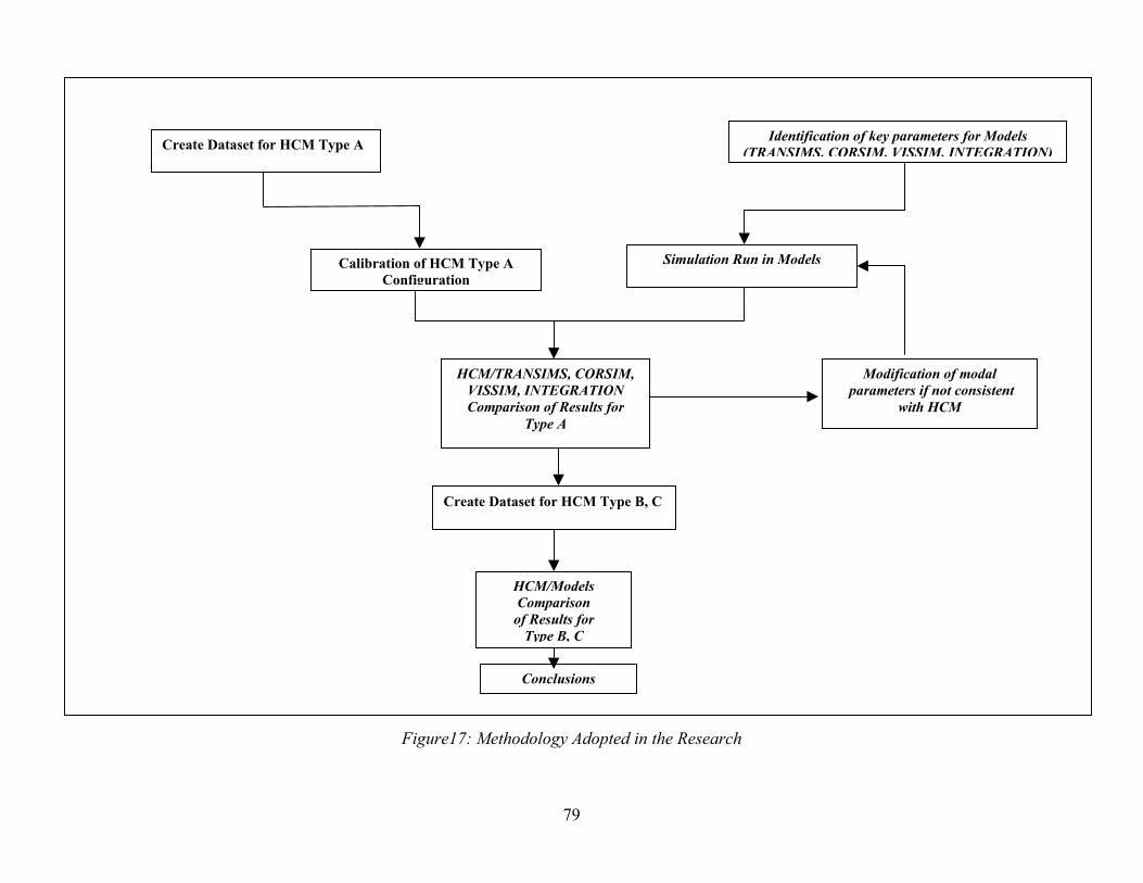
79

Create Dataset for HCM Type A

Create Dataset for HCM Type B, C

Calibration of HCM Type A Configuration

Identification of key parameters for Models (TRANSIMS, CORSIM, VISSIM, INTEGRATION)

HCM/TRANSIMS, CORSIM, VISSIM, INTEGRATION Comparison of Results for

Type A

Simulation Run in Models

Modification of modal parameters if not consistent

with HCM

HCM/Models Comparison of Results for

Type B, C

Conclusions

Figure17: Methodology Adopted in the Research

3.3 The Modeling Concepts

3.3.1 HCM The traditional models like HCM predict volumes immediately upstream of the ramp

junction. The prediction is based upon full hour volumes and is calculated in mixed

vehicles per hour (vph). Such models, while simple and straightforward in prediction of

volumes, are complex, when applied to capacity analysis.

• Traditional HCM models focus on volume as input and evaluate the speed as an

output for the entire weaving section.

• The HCM is based upon analysis of flow rates within 30-minutes periods of time. To

conform to other methodologies in HCM, 30-minute data periods are used in all the

models studied.

• All calibrations are made in passenger car equivalents (pce’s).

In the context of the proposed model, several changes have been made to incorporate a

similar model existing in HCM as described in the following subsections.

3.3.2 TRANSIMS Some of the standard assumptions made in TRANSIMS

• The link is divided into 7.5-meter cells.

• The vehicles moving on the links are of the types specified by the vehicle prototype

file. They comprise of autos that occupy one cell or trucks that occupy two cells. The

file also states their maximum acceleration and speeds possible for each vehicle type.

• HCM predicts the weaving speed and non-weaving speed per vehicle. The result is

obtained from the TRANSIMS Microsimulator in the form of the snapshot data. Thus

snapshot data is processed to interpret the results.

To develop a scenario similar to Highway Capacity Manual, all of the necessary tables

for the network are coded manually. The network is split into a combination of nodes and

links, parking being provided at each entry and exit point of the links, from where

80

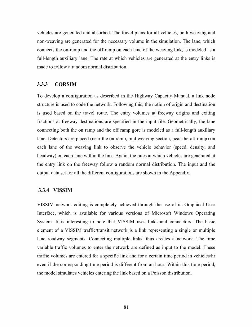
vehicles are generated and absorbed. The travel plans for all vehicles, both weaving and

non-weaving are generated for the necessary volume in the simulation. The lane, which

connects the on-ramp and the off-ramp on each lane of the weaving link, is modeled as a

full-length auxiliary lane. The rate at which vehicles are generated at the entry links is

made to follow a random normal distribution.

3.3.3 CORSIM To develop a configuration as described in the Highway Capacity Manual, a link node

structure is used to code the network. Following this, the notion of origin and destination

is used based on the travel route. The entry volumes at freeway origins and exiting

fractions at freeway destinations are specified in the input file. Geometrically, the lane

connecting both the on ramp and the off ramp gore is modeled as a full-length auxiliary

lane. Detectors are placed (near the on ramp, mid weaving section, near the off ramp) on

each lane of the weaving link to observe the vehicle behavior (speed, density, and

headway) on each lane within the link. Again, the rates at which vehicles are generated at

the entry link on the freeway follow a random normal distribution. The input and the

output data set for all the different configurations are shown in the Appendix.

3.3.4 VISSIM

VISSIM network editing is completely achieved through the use of its Graphical User

Interface, which is available for various versions of Microsoft Windows Operating

System. It is interesting to note that VISSIM uses links and connectors. The basic

element of a VISSIM traffic/transit network is a link representing a single or multiple

lane roadway segments. Connecting multiple links, thus creates a network. The time

variable traffic volumes to enter the network are defined as input to the model. These

traffic volumes are entered for a specific link and for a certain time period in vehicles/hr

even if the corresponding time period is different from an hour. Within this time period,

the model simulates vehicles entering the link based on a Poisson distribution.

81

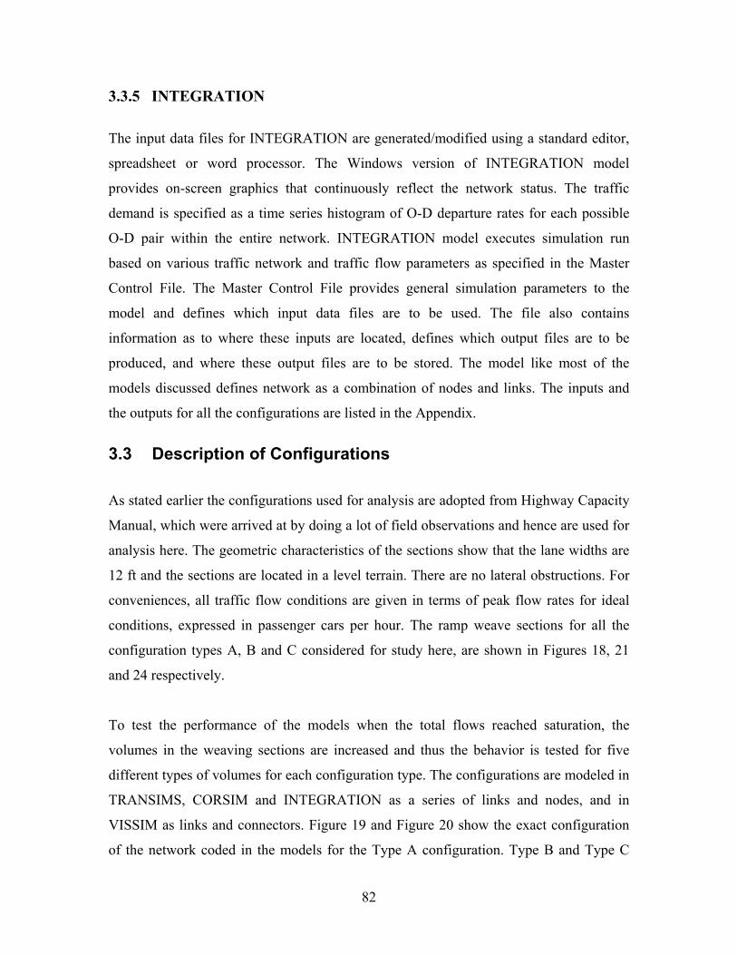
3.3.5 INTEGRATION

The input data files for INTEGRATION are generated/modified using a standard editor,

spreadsheet or word processor. The Windows version of INTEGRATION model

provides on-screen graphics that continuously reflect the network status. The traffic

demand is specified as a time series histogram of O-D departure rates for each possible

O-D pair within the entire network. INTEGRATION model executes simulation run

based on various traffic network and traffic flow parameters as specified in the Master

Control File. The Master Control File provides general simulation parameters to the

model and defines which input data files are to be used. The file also contains

information as to where these inputs are located, defines which output files are to be

produced, and where these output files are to be stored. The model like most of the

models discussed defines network as a combination of nodes and links. The inputs and

the outputs for all the configurations are listed in the Appendix.

3.3 Description of Configurations

As stated earlier the configurations used for analysis are adopted from Highway Capacity

Manual, which were arrived at by doing a lot of field observations and hence are used for

analysis here. The geometric characteristics of the sections show that the lane widths are

12 ft and the sections are located in a level terrain. There are no lateral obstructions. For

conveniences, all traffic flow conditions are given in terms of peak flow rates for ideal

conditions, expressed in passenger cars per hour. The ramp weave sections for all the

configuration types A, B and C considered for study here, are shown in Figures 18, 21

and 24 respectively.

To test the performance of the models when the total flows reached saturation, the

volumes in the weaving sections are increased and thus the behavior is tested for five

different types of volumes for each configuration type. The configurations are modeled in

TRANSIMS, CORSIM and INTEGRATION as a series of links and nodes, and in

VISSIM as links and connectors. Figure 19 and Figure 20 show the exact configuration

of the network coded in the models for the Type A configuration. Type B and Type C

82

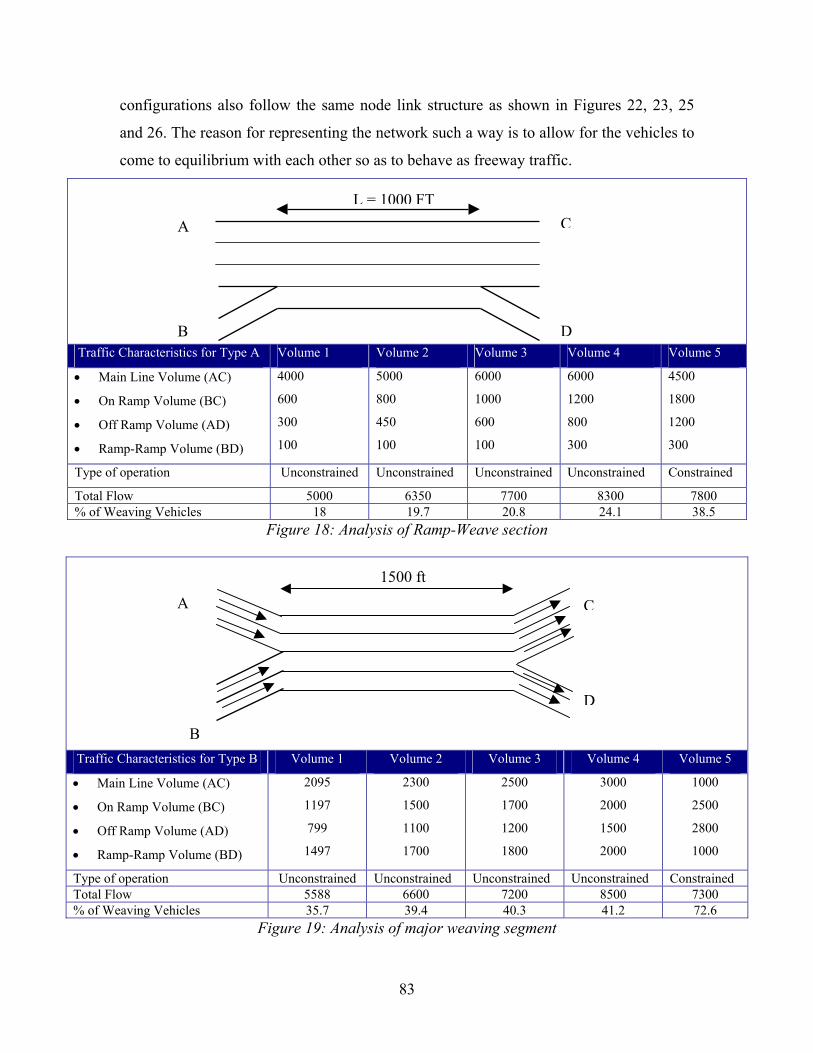
configurations also follow the same node link structure as shown in Figures 22, 23, 25

and 26. The reason for representing the network such a way is to allow for the vehicles to

come to equilibrium with each other so as to behave as freeway traffic.

Traffic Characteristics for Type A Volume 1 Volume 2 Volume 3 Volume 4 Volume 5

• Main Line Volume (AC)

• On Ramp Volume (BC)

• Off Ramp Volume (AD)

• Ramp-Ramp Volume (BD)

4000

600

300

100

5000

800

450

100

6000

1000

600

100

6000

1200

800

300

4500

1800

1200

300

Type of operation Unconstrained Unconstrained Unconstrained Unconstrained Constrained

Total Flow 5000 6350 7700 8300 7800 % of Weaving Vehicles 18 19.7 20.8 24.1 38.5

L = 1000 FTC

D

A

B

Figure 18: Analysis of Ramp-Weave section

Traffic Characteristics for Type B Volume 1 Volume 2 Volume 3 Volume 4 Volume 5

• Main Line Volume (AC)

• On Ramp Volume (BC)

• Off Ramp Volume (AD)

• Ramp-Ramp Volume (BD)

2095

1197

799

1497

2300

1500

1100

1700

2500

1700

1200

1800

3000

2000

1500

2000

1000

2500

2800

1000

Type of operation Unconstrained Unconstrained Unconstrained Unconstrained Constrained Total Flow 5588 6600 7200 8500 7300 % of Weaving Vehicles 35.7 39.4 40.3 41.2 72.6

1500 ft

C

D

A

B

Figure 19: Analysis of major weaving segment

83

Traffic Characteristics for Type B Volume 1 Volume 2 Volume 3 Volume 4 Volume 5

• Main Line Volume (AC)

• On Ramp Volume (BC)

• Off Ramp Volume (AD)

• Ramp-Ramp Volume (BD)

2000

1500

1450

2000

3500

300

200

3500

4000

350

300

4000

1200

900

850

1200

1600

1300

1250

1600

Type of operation Unconstrained Unconstrained Constrained Constrained Constrained Total Flow 7500 8650 4150 5750 6950 % of Weaving Vehicles 6.7 7.5 42.2 44.3 42.4

A C

B D

1000 ft

Figure 20: Analysis of Alternative Major Weaving Segments

84

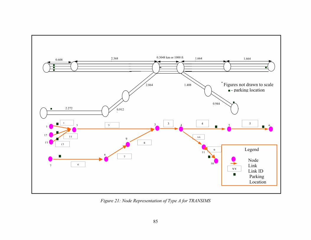
* Figures not drawn to scale- parking location

0.608 k

2.368 k

0.3048 km or 1000 ft 1.664 k

1.664 k

2.864 k

1.408 k

0.912 k

2.272 k

0.944 k

Legend Node Link Link ID

Parking Location

1

12

13

2 3 4 5 6

9

11

1

11

12

23

8

4

10

5

XX

7

6

9

7

8

10

Figure 21: Node Representation of Type A for TRANSIMS

85

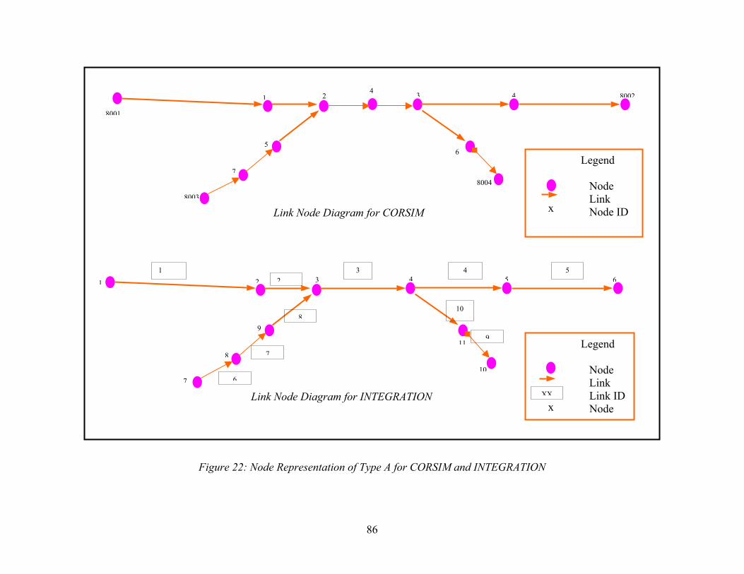
Legend Node Link Node ID

8001

1 2 3 4 8002

5

Link Node Diagram for CORSIM 8003

7

4

6

8004

x

Legend Node Link Link ID Node

1 2 3 4 5 6

9

11

1 2

3

8

4

10

5

XXLink Node Diagram for INTEGRATION

7

6

9

7

8

10

x

Figure 22: Node Representation of Type A for CORSIM and INTEGRATION

86

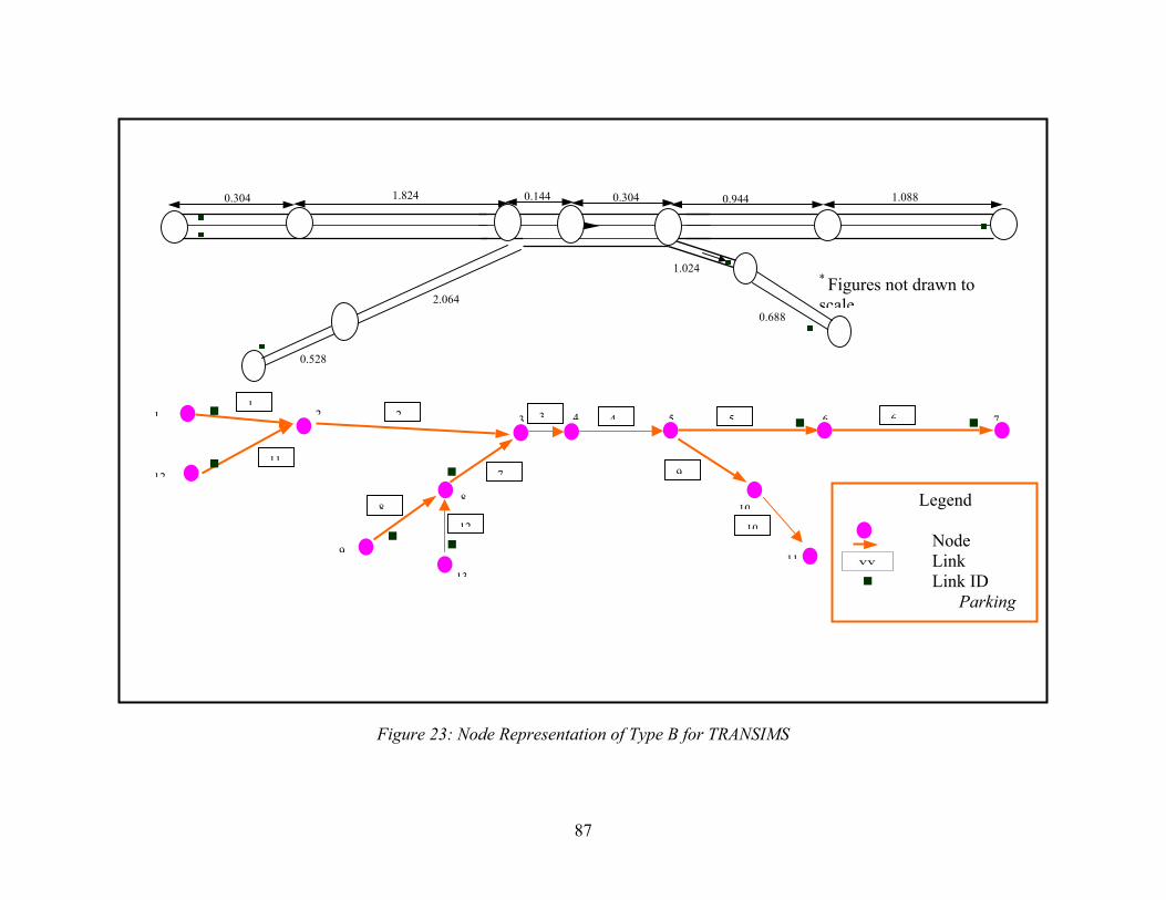
* Figures not drawn to scale

0.304 1.824 0.944 1.088

2.064

1.024

0.528

0.688

0.144 0.304

Legend Node Link Link ID

Parking

1

12

2 3 5 6 7

810

XX

4

9

1311

1

11

2 3 4

8

5 6

12

7 9

10

Figure 23: Node Representation of Type B for TRANSIMS

87

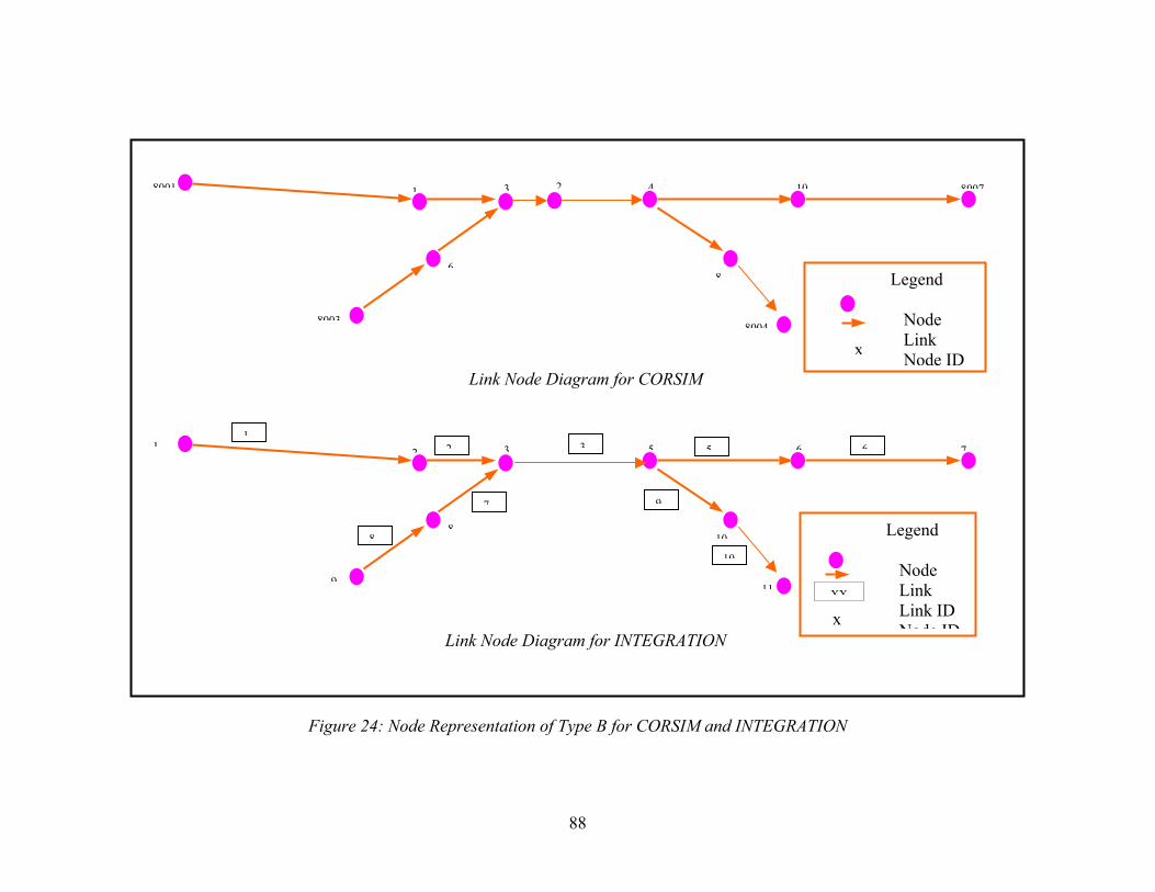
Link Node Diagram for CORSIM

Legend Node Link

Node ID

8001 1 3 4 10 8007

68

2

8003 8004

x

Legend Node Link Link ID

Node ID

1 2 3 5 6 7

810

XX

Link Node Diagram for INTEGRATION

911

12 3

8

5 6

7 9

10

x

Figure 24: Node Representation of Type B for CORSIM and INTEGRATION

88

* Figures not drawn to scale

0.304 1.824 0.944 1.088

2.064

1.024

0.528

0.688

0.144 0.144

Legend Node Link Link ID

Parking Location

1

12

2 3 5 6 7

810

XX

4

9

1311

1

11

2 3 4

8

5 6

12

7 9

10

Figure 25: Node Representation of Type C for TRANSIMS

89

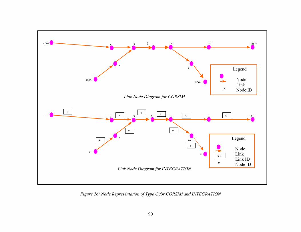
Link Node Diagram for CORSIM

Legend Node Link Node ID

8001 1 3 4 10 8007

68

2

80038004

x

Legend Node Link Link ID

Node ID

1 2 3 5 6 7

810

XX

Link Node Diagram for INTEGRATION

911

12

3

8

5 6

7 9

1

x

44

Figure 26: Node Representation of Type C for CORSIM and INTEGRATION

90

Chapter 4: Comparing HCM, TRANSIMS, CORSIM, VISSIM and INTEGRATION Results

A basis for the comparison of results between HCM, TRANSIMS, CORSIM, VISSIM

and INTEGRATION is needed, and hence a common data set is created for all the

models. Taking HCM as the base model and assuming similar traffic and geometric

conditions for all the models, sensitivity analysis is conducted for Type A configuration

of the weaving section. This is done to assess the applicability of all the models to the

model in HCM and then the same values are used for the other two types of

configurations. Although it is not recommended to use the HCM results as baseline, this

is done only for the model validation of this experimental study, as there is no field data

available to calibrate the model. The results obtained for all the models are then

compared to the base model.

4.1 Calibration Parameters for the Models

The following sections identify the key parameters or configuration keys for the models.

A series of test simulations are conducted changing each of the parameters identified,

then studying the results and interpreting how they affect the model. The Type A

configuration of the ramp-weave section is used for model calibration and sensitivity

analysis. After these runs, the model with calibrated parameters that best describes the

scenario is chosen and the other types of configurations simulated. For every case three

simulation runs are considered so as to average out the error or bring them closer to the

true expected values. The statistics collected over these tests include the average speeds

of weaving and non-weaving vehicles and the average densities given by each of these

configurations.

4.1.1 TRANSIMS The parameters influencing the behavior of vehicles in the freeway weaving sections in

TRANSIMS are identified as deceleration probability, lane change probability and

91

planning ahead for a lane change which are discussed in detail in the following

subsections.

Deceleration Probability

The configuration key CA_DECELERATION_PROBABILITY defines the probability of a

driver to decelerate for no reason. This enhances the traffic variation as each automobile

driver randomly decides whether to decelerate for no apparent reason at each timestep.

This configuration key is defined by the user and it assumes a value between 0.0 and 1.0.

If the configuration key is set to 0, it would mean that a driver would never decelerate

without a reason. The only time he/she would decelerate would be when the gap ahead of

him/her is less than the velocity at which he/she is driving. If this key is set to 1 it would

imply that a driver would always decelerate at every timestep where the gap ahead of

him/her is more than the velocity.

This configuration key is important as it replicates human behavior for not accelerating

all the time. As stated earlier for a model to depict reality, it is very important to capture

such kind of data and calibrate the model. For the sake of this study, since no real world

data on weaving sections was present the model was calibrated to that of a default value

of 0.2. This implies that one-fifth of the time a driver would decelerate for no apparent

reason. This value is also justified as the default value was arrived at in TRANSIMS

based on several studies conducted by the research team headed by Kai Nagel. (Jillella et

al., 2001)

Lane Change Probability

The configuration key that controls a lane-changing maneuver is the

CA_LANE_CHANGE_PROBABILTIY. Should all the conditions be satisfied for a driver to

lane change into the adjacent lane, this configuration key specifies the probability of the

driver to lane change i.e., should a slower vehicle be ahead of a vehicle whose gap ahead

is less than the velocity at which it is traveling and the gap ahead in the adjacent lane is

more than in the current lane while the gap behind in the new lane is more than the

VGlobalMax, then all the conditions are satisfied for a lane change. It should also be noted

92

that right and left lane changes occur on alternate timesteps. Having all the condition

satisfied for a lane change a driver would still only lane change with a probability given

by this configuration key. This configuration key is quite crucial for the simulation to

perform close to reality. An example to emphasize the importance of this key would be to

consider a two-lane roadway with all the vehicles in one lane next to each other. This

would mean that every vehicle would have its conditions for lane change based on gaps

fulfilled. So in the next time step each of the vehicles would move into the adjacent lane.

This continues at every timestep and would result in very unrealistic scenario.

Introducing this configuration key helps stabilize this maneuver.

As the configuration key suggests, it represents the probability of lane change and so the

permissible values lie between 0 and 1. A default value of 0.99 was arrived at after a lot

of experimental studies at the Los Alamos National Laboratories and is used in this

research too.

Planning ahead for a lane change

For this study it is important that drivers plan ahead for a lane change as the drivers are

constrained by time and distance to get into the right lanes. The configurations keys

discussed in this subsection could be thought of as off-ramp information signs for drivers

that have to go off-ramp.

TRANSIMS Microsimulator uses two configuration keys for modeling this behavior. The

first of which is the CA_PLAN_FOLLOWING_CELLS. This configuration key specifies the

number of cells preceding the intersection within which a vehicle will make a lane

change to get into the appropriate lane and thus transition into the next link in its plan.

Beyond this distance any lane changes are based only on vehicle speed and gaps in the

traffic. Within this distance, the lane required by vehicle’s plan is also taken into account.

As the vehicle nears the intersection, the bias to be in the lane required to stay on plan is

increased. The valid values for this configuration key are positive values or zero.

93

The second configuration key that helps in planning ahead for a lane change is the

CA_LOOK_AHEAD_CELLS. To understand the significance of this configuration key it

should be noted that the preferred lane for a vehicle to be in as it approaches an

intersection depends on the connectivity from the current link to the next link in the plan.

In certain cases it would be advantageous for the driver to look beyond the next link to

the subsequent links in the plan when deciding the preferred lane. This configuration key

controls how far ahead the driver will look beyond the next link. A positive value set for

the configuration key indicates that the driver would look at least one additional step

beyond the next step in the plan. The number of additional links considered is determined

by the lengths of the subsequent links.

These configuration keys again have to be calibrated for the study. Since the study area

configuration of the network is known, sensitivity analysis on these configuration keys is

performed. (Jillella et al., 2001)

4.1.2 CORSIM The parameters considered to influence the lane changing behavior, thus affecting the

weaving maneuvers of the vehicles in the weaving sections in CORSIM, are off-ramp

warning sign distance, driver characteristics like time required to maneuver to correct

lane, and percentage of drivers yielding to lane change.

Off-ramp warning sign distance

The off - ramp warning sign distance is defined as the distance from the point where the

warning sign is positioned in relation to the downstream end of the link, at which drivers

begin to react to the off – ramp exiting from the link. Hence this parameter details how

far of the upstream from the downstream end of the link the vehicles are destined to exit

at the off-ramp, begin to react to the exit's presence. The vehicle will start to enter the

lane when it is at this distance. The default value used in CORSIM is 2500 ft. This value

is specified in Record Type 20.

94

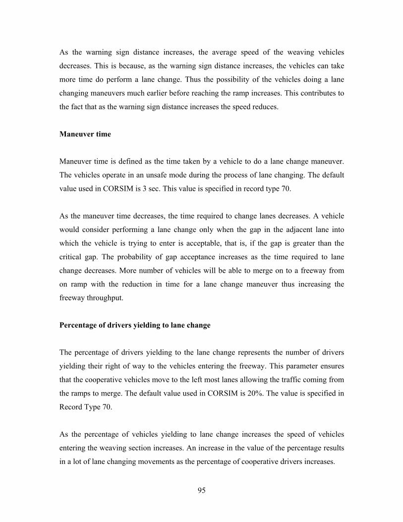
As the warning sign distance increases, the average speed of the weaving vehicles

decreases. This is because, as the warning sign distance increases, the vehicles can take

more time do perform a lane change. Thus the possibility of the vehicles doing a lane

changing maneuvers much earlier before reaching the ramp increases. This contributes to

the fact that as the warning sign distance increases the speed reduces.

Maneuver time

Maneuver time is defined as the time taken by a vehicle to do a lane change maneuver.

The vehicles operate in an unsafe mode during the process of lane changing. The default

value used in CORSIM is 3 sec. This value is specified in record type 70.

As the maneuver time decreases, the time required to change lanes decreases. A vehicle

would consider performing a lane change only when the gap in the adjacent lane into

which the vehicle is trying to enter is acceptable, that is, if the gap is greater than the

critical gap. The probability of gap acceptance increases as the time required to lane

change decreases. More number of vehicles will be able to merge on to a freeway from

on ramp with the reduction in time for a lane change maneuver thus increasing the

freeway throughput.

Percentage of drivers yielding to lane change

The percentage of drivers yielding to the lane change represents the number of drivers

yielding their right of way to the vehicles entering the freeway. This parameter ensures

that the cooperative vehicles move to the left most lanes allowing the traffic coming from

the ramps to merge. The default value used in CORSIM is 20%. The value is specified in

Record Type 70.

As the percentage of vehicles yielding to lane change increases the speed of vehicles

entering the weaving section increases. An increase in the value of the percentage results

in a lot of lane changing movements as the percentage of cooperative drivers increases.

95

4.1.3 VISSIM The parameters influencing the weaving behavior of vehicles in weaving sections in

VISSIM include link connection and time steps per simulation second.

Link Connection

This parameter defines the distance at which vehicles will begin to attempt to change

lanes in order to exit a ramp. The default value used in VISSIM is 200 m. A value of

1000 m is used in all the simulation runs after having consulted with the VISSIM

software development research group at itc-world who arrived at this figure after a lot of

field observations.

Time steps per simulation second

The parameter indicates the number of times the position of the vehicle will be calculated

within one simulated second (it follows a range of 1 to 10). An input of 1 will result in

the movement of vehicles once a simulated second. An input of 10 will result in the

movement of the vehicles to be more smooth as all vehicle movements will be calculated

10 times per simulation second. It has been found out that the change of simulation speed

is inversely proportional to the time steps. A default value of 1 is used in VISSIM but for

the present study a value of 10 is considered as per the recommendation of the VISSIM

software development group.

4.1.4 INTEGRATION Lane Bias File

A lane bias file is an optional file that biases vehicles to change lanes within a specified

distance of a downstream link. The optional input file is named as ‘lanebias.dat’. The

parameters included in the file will override the lane bias internal to the model. The file is

important as it replicates the usage of a particular lane, thus governing the behavior of the

movement of the vehicles. As stated earlier for a model to depict reality, it is very

96

important to capture such kind of data. For the sake of this study, since no real world data

on weaving sections is present this optional file is not specified. The lane bias internal to

the model is used for simulation runs.

Time-Space diagrams for a typical vehicle for TRANSIMS, CORSIM, VISSIM and

INTEGRATION

A better understanding of the particle hopping theory, car following theory as well as the

actual movements of the vehicles could be understood with time-space figures. The time-

space diagrams for the Type A configuration is presented below for all the models and

since the distance of vehicle movements is closely related to the velocity, a plot of the

velocity on the same figure is shown. The data for the figures plotted is attached in the

Appendix.

The figures shown below depict a single vehicles path as it traverses the weaving section

for through, offramp, onramp and ramp-ramp vehicles. The x-axis on these graphs

represents the time. It is assumed that the time at which the vehicle enters the weaving

section is 0 and the trajectory is presented till the time it moves off the weaving section.

The data is shown in points in accordance with the car following theory.

Ramp - Ramp vehicle

0

100

200

300

400

0 5 10 15Time (sec)

DistanceSpeed

Dis

tanc

e (m

); Sp

eed

(m/s

) Through Vehicle

050

100150200250300350

0 5 10 15Time (sec)

Distance

Speed

Dis

tanc

e (m

); Sp

eed

(m/s

)

97

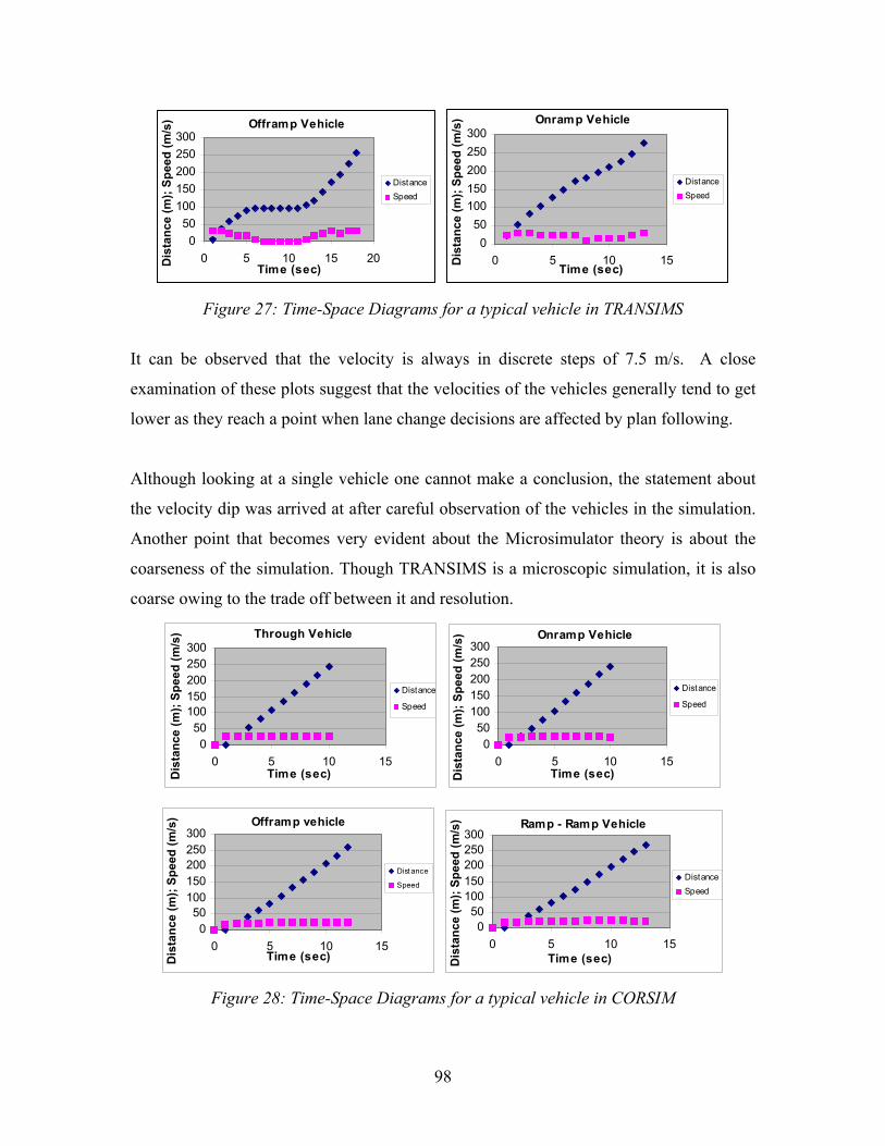
Offramp Vehicle

050

100150200250300

0 5 10 15 20Time (sec)

DistanceSpeed

Dis

tanc

e (m

); Sp

eed

(m/s

) Onramp Vehicle

050

100150200250300

0 5 10 15Time (sec)

DistanceSpeed

Dis

tanc

e (m

); Sp

eed

(m/s

)

Figure 27: Time-Space Diagrams for a typical vehicle in TRANSIMS

It can be observed that the velocity is always in discrete steps of 7.5 m/s. A close

examination of these plots suggest that the velocities of the vehicles generally tend to get

lower as they reach a point when lane change decisions are affected by plan following.

Although looking at a single vehicle one cannot make a conclusion, the statement about

the velocity dip was arrived at after careful observation of the vehicles in the simulation.

Another point that becomes very evident about the Microsimulator theory is about the

coarseness of the simulation. Though TRANSIMS is a microscopic simulation, it is also

coarse owing to the trade off between it and resolution.

Through Vehicle

050

100150200250300

0 5 10 15Time (sec)

Distance

Speed

Dis

tanc

e (m

); Sp

eed

(m/s

) Onramp Vehicle

050

100150200250300

0 5 10 15Time (sec)

Distance

Speed

Dis

tanc

e (m

); Sp

eed

(m/s

)

Offramp vehicle

050

100150200250300

0 5 10 15Time (sec)

Dist ance

Speed

Dis

tanc

e (m

); Sp

eed

(m/s

) Ramp - Ramp Vehicle

050

100150200250300

0 5 10 15Time (sec)

DistanceSpeed

Dis

tanc

e (m

); Sp

eed

(m/s

)

Figure 28: Time-Space Diagrams for a typical vehicle in CORSIM

98

The time space plots for a single vehicle in CORSIM show that the speeds of the vehicles

are almost constant during their travel in the weaving section. It does not demonstrate any

queue built up in the section thus representing a smooth flow of traffic. Although the

behavior of a single vehicle is not representative of the performance of the considered

volume of vehicles being simulated, it was noticed from the simulation that there was no

erratic behavior of the vehicles traveling on these sections.

Through Vehicle

0

50

100

150

200

250

300

350

0 2 4 6 8 10 12Time (sec)

Distance

Speed

Dis

tanc

e (m

); Sp

eed

(m/s

) Offramp Vehicle

0

50

100

150

200

250

300

0 5 10 15Time (sec)

Dist ance

Speed

Dis

tanc

e (m

); Sp

eed

(m/s

)

Onramp Vehicle

0

50

100

150

200

250

300

0 5 10 15Time

Dist ance

Speed

Dis

tanc

e (m

); Sp

eed

(m/s

)

Ramp - Ramp Vehicle

0

50

100

150

200

250

300

0 5 10 15Time (sec)

Dist ance

Speed

Dis

tanc

e (m

); Sp

eed

(m/s

)

Figure 29: Time-Space Diagrams for a typical vehicle in VISSIM

The time space plots for a single vehicle in VISSIM show that the speeds of the vehicles

are increasing and decreasing with a very slight variation which is very much

representative of the real world scenario considering the lane changing maneuvers and

anticipatory lane changes and weaving movements.

99

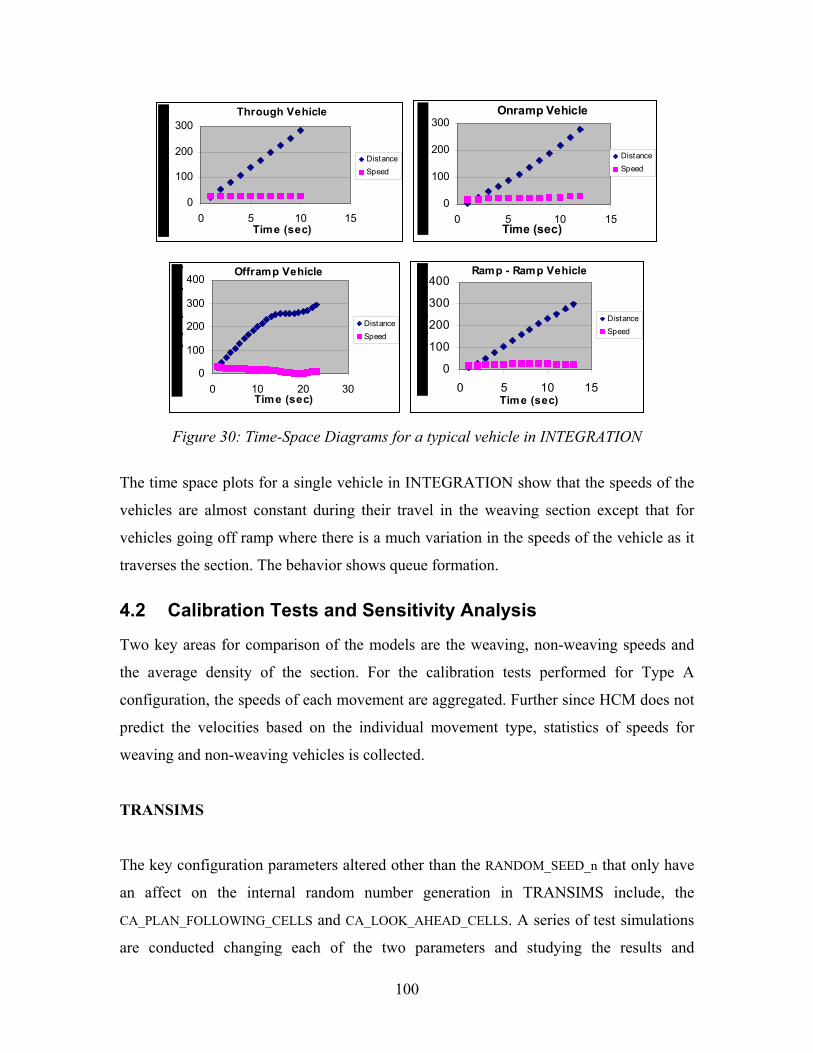
Through Vehicle

0

100

200

300

0 5 10 15Time (sec)

DistanceSpeed

Onramp Vehicle

0

100

200

300

0 5 10 15Time (sec)

DistanceSpeed

Offramp Vehicle

0

100

200

300

400

0 10 20 30Time (sec)

DistanceSpeed

Ramp - Ramp Vehicle

0

100

200

300

400

0 5 10 15Time (sec)

DistanceSpeed

Figure 30: Time-Space Diagrams for a typical vehicle in INTEGRATION

The time space plots for a single vehicle in INTEGRATION show that the speeds of the

vehicles are almost constant during their travel in the weaving section except that for

vehicles going off ramp where there is a much variation in the speeds of the vehicle as it

traverses the section. The behavior shows queue formation.

4.2 Calibration Tests and Sensitivity Analysis

Two key areas for comparison of the models are the weaving, non-weaving speeds and

the average density of the section. For the calibration tests performed for Type A

configuration, the speeds of each movement are aggregated. Further since HCM does not

predict the velocities based on the individual movement type, statistics of speeds for

weaving and non-weaving vehicles is collected.

TRANSIMS

The key configuration parameters altered other than the RANDOM_SEED_n that only have

an affect on the internal random number generation in TRANSIMS include, the

CA_PLAN_FOLLOWING_CELLS and CA_LOOK_AHEAD_CELLS. A series of test simulations

are conducted changing each of the two parameters and studying the results and

100

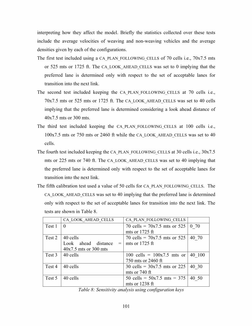
interpreting how they affect the model. Briefly the statistics collected over these tests

include the average velocities of weaving and non-weaving vehicles and the average

densities given by each of the configurations.

The first test included using a CA_PLAN_FOLLOWING_CELLS of 70 cells i.e., 70x7.5 mts

or 525 mts or 1725 ft. The CA_LOOK_AHEAD_CELLS was set to 0 implying that the

preferred lane is determined only with respect to the set of acceptable lanes for

transition into the next link.

The second test included keeping the CA_PLAN_FOLLOWING_CELLS at 70 cells i.e.,

70x7.5 mts or 525 mts or 1725 ft. The CA_LOOK_AHEAD_CELLS was set to 40 cells

implying that the preferred lane is determined considering a look ahead distance of

40x7.5 mts or 300 mts.

The third test included keeping the CA_PLAN_FOLLOWING_CELLS at 100 cells i.e.,

100x7.5 mts or 750 mts or 2460 ft while the CA_LOOK_AHEAD_CELLS was set to 40

cells.

The fourth test included keeping the CA_PLAN_FOLLOWING_CELLS at 30 cells i.e., 30x7.5

mts or 225 mts or 740 ft. The CA_LOOK_AHEAD_CELLS was set to 40 implying that

the preferred lane is determined only with respect to the set of acceptable lanes for

transition into the next link.

The fifth calibration test used a value of 50 cells for CA_PLAN_FOLLOWING_CELLS. The

CA_LOOK_AHEAD_CELLS was set to 40 implying that the preferred lane is determined

only with respect to the set of acceptable lanes for transition into the next link. The

tests are shown in Table 8.

CA_LOOK_AHEAD_CELLS CA_PLAN_FOLLOWING_CELLS Test 1 0

70 cells = 70x7.5 mts or 525 mts or 1725 ft

0_70

Test 2 40 cells Look ahead distance = 40x7.5 mts or 300 mts

70 cells = 70x7.5 mts or 525 mts or 1725 ft

40_70

Test 3 40 cells 100 cells = 100x7.5 mts or 750 mts or 2460 ft

40_100

Test 4 40 cells 30 cells = 30x7.5 mts or 225 mts or 740 ft

40_30

Test 5 40 cells 50 cells = 50x7.5 mts = 375 mts or 1238 ft

40_50

Table 8: Sensitivity analysis using configuration keys

101

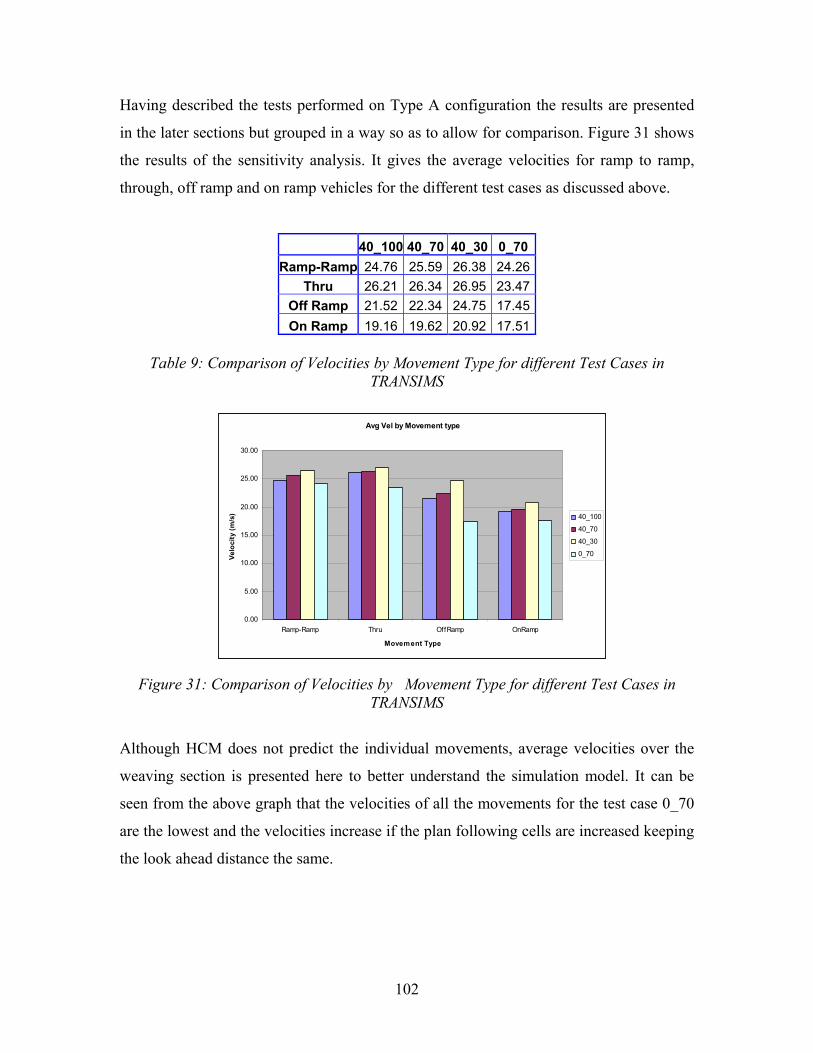
Having described the tests performed on Type A configuration the results are presented

in the later sections but grouped in a way so as to allow for comparison. Figure 31 shows

the results of the sensitivity analysis. It gives the average velocities for ramp to ramp,

through, off ramp and on ramp vehicles for the different test cases as discussed above.

40_100 40_70 40_30 0_70Ramp-Ramp 24.76 25.59 26.38 24.26

Thru 26.21 26.34 26.95 23.47Off Ramp 21.52 22.34 24.75 17.45On Ramp 19.16 19.62 20.92 17.51

Table 9: Comparison of Velocities by Movement Type for different Test Cases in

TRANSIMS

Avg Vel by Movement type

0.00

5.00

10.00

15.00

20.00

25.00

30.00

Ramp-Ramp Thru OffRamp OnRamp

Movement Type

Velo

city

(m/s

) 40_100

40_70

40_30

0_70

Figure 31: Comparison of Velocities by Movement Type for different Test Cases in TRANSIMS

Although HCM does not predict the individual movements, average velocities over the

weaving section is presented here to better understand the simulation model. It can be

seen from the above graph that the velocities of all the movements for the test case 0_70

are the lowest and the velocities increase if the plan following cells are increased keeping

the look ahead distance the same.

102

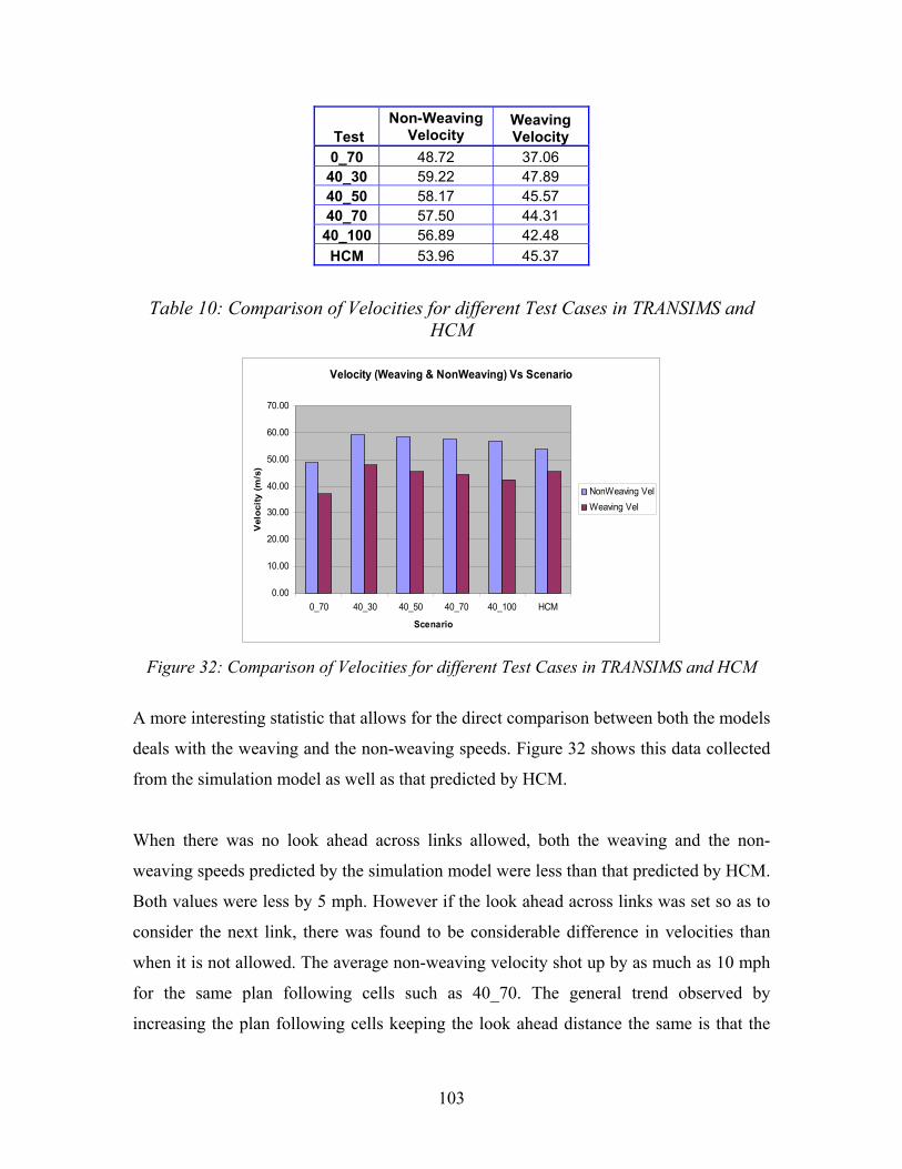
Test Non-Weaving

Velocity Weaving Velocity

0_70 48.72 37.06 40_30 59.22 47.89 40_50 58.17 45.57 40_70 57.50 44.31 40_100 56.89 42.48 HCM 53.96 45.37

Table 10: Comparison of Velocities for different Test Cases in TRANSIMS and HCM

Velocity (Weaving & NonWeaving) Vs Scenario

0.00

10.00

20.00

30.00

40.00

50.00

60.00

70.00

0_70 40_30 40_50 40_70 40_100 HCM

Scenario

Vel

ocity

(m/s

)

NonWeaving VelWeaving Vel

Figure 32: Comparison of Velocities for different Test Cases in TRANSIMS and HCM

A more interesting statistic that allows for the direct comparison between both the models

deals with the weaving and the non-weaving speeds. Figure 32 shows this data collected

from the simulation model as well as that predicted by HCM.

When there was no look ahead across links allowed, both the weaving and the non-

weaving speeds predicted by the simulation model were less than that predicted by HCM.

Both values were less by 5 mph. However if the look ahead across links was set so as to

consider the next link, there was found to be considerable difference in velocities than

when it is not allowed. The average non-weaving velocity shot up by as much as 10 mph

for the same plan following cells such as 40_70. The general trend observed by

increasing the plan following cells keeping the look ahead distance the same is that the

103

non-weaving and the weaving speeds are reduced. For all the test cases considered the

non-weaving speeds were slightly higher in the simulation than those predicted by HCM

while the weaving speeds were slightly less than those predicted by HCM.

The second output variable where the simulation model is compared to HCM is the

average density. The results aggregated from the simulation runs and the values predicted

by HCM are shown in Figure 33.

Average Density0_70 26.60 40_30 21.53 40_50 21.79 40_70 22.19 40_100 22.88 HCM 23.96

Table 11: Comparison of Densities for Test Cases in TRANSIMS and HCM

Average Density vs Scenario

0.00

5.00

10.00

15.00

20.00

25.00

30.00

0_70 40_30 40_50 40_70 40_100 HCM

Scenario

Ave

rage

Den

sity

Average Density

Figure 33: Comparison of Densities for different Test Cases in TRANSIMS and HCM

The average density for the first calibration test (0_70) had the highest density among all

the tests. The value was found to be higher than the one predicted by HCM. For the rest

104

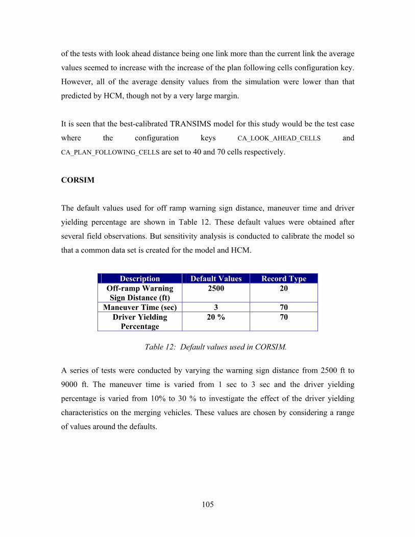
of the tests with look ahead distance being one link more than the current link the average

values seemed to increase with the increase of the plan following cells configuration key.

However, all of the average density values from the simulation were lower than that

predicted by HCM, though not by a very large margin.

It is seen that the best-calibrated TRANSIMS model for this study would be the test case

where the configuration keys CA_LOOK_AHEAD_CELLS and

CA_PLAN_FOLLOWING_CELLS are set to 40 and 70 cells respectively.

CORSIM

The default values used for off ramp warning sign distance, maneuver time and driver

yielding percentage are shown in Table 12. These default values were obtained after

several field observations. But sensitivity analysis is conducted to calibrate the model so

that a common data set is created for the model and HCM.

Description Default Values Record Type Off-ramp Warning Sign Distance (ft)

2500 20

Maneuver Time (sec) 3 70 Driver Yielding

Percentage 20 % 70

Table 12: Default values used in CORSIM.

A series of tests were conducted by varying the warning sign distance from 2500 ft to

9000 ft. The maneuver time is varied from 1 sec to 3 sec and the driver yielding

percentage is varied from 10% to 30 % to investigate the effect of the driver yielding

characteristics on the merging vehicles. These values are chosen by considering a range

of values around the defaults.

105

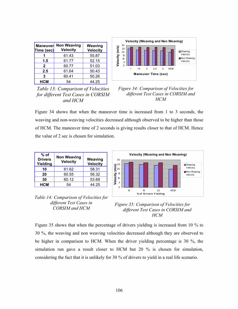
Velocity (Weaving and Non Weaving)

05

1015

202530

1 1.5 2 2.5 3 HCM

Maneuver Time (sec)

Velo

city

(m/s

)

WeavingVelocityNon WeavingVelocity

Table 13: Comparison of Velocities

Maneuver Time (sec)

Non Weaving Velocity

Weaving Velocity

1 61.43 55.87 1.5 61.77 52.15

2 60.77 51.03 2.5 61.64 50.43

3 60.41 50.26 HCM 54 44.25

f

Figure 34 shows that when the maneuver time is increased from 1 to 3 seconds, the

weaving and non-weaving velocities decreased although observed to be higher than those

of HCM. The maneuver time of 2 seconds is giving results closer to that of HCM. Hence

the value of 2 sec is chosen for simulation.

Velocity (Weaving and Non Weaving)

0

5

10

15

20

25

30

10 15 20 HCM% o f D rivers Y ield ing

Velo

city

(m/s

) WeavingVelocity

Non Weavingvelocity

% of Drivers Yielding

Non Weaving Velocity Weaving

Velocity 10 61.62 58.31 20 60.55 56.32 30 60.12 53.69

HCM 54 44.25

or different Test Cases in CORSIM and HCM

Figure 35: Comparison of Velocities for different Test Cases in CORSIM and

HCM

Table 14: Comparison of Velocities for different Test Cases in

CORSIM and HCM

Figure 34: Comparison of Velocities for different Test Cases in CORSIM and

HCM

Figure 35 shows that when the percentage of drivers yielding is increased from 10 % to

30 %, the weaving and non weaving velocities decreased although they are observed to

be higher in comparison to HCM. When the driver yielding percentage is 30 %, the

simulation run gave a result closer to HCM but 20 % is chosen for simulation,

considering the fact that it is unlikely for 30 % of drivers to yield in a real life scenario.

106

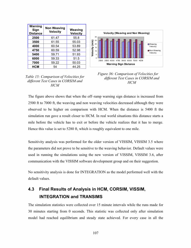
Velocity (Weaving and Non Weaving)

0

5

10

15

20

25

30

2500 3500 4000 4750 5400 6000 7000 HCM

Warning Sign Distance

Velo

city

(m/s

)

WeavingVelocity

Non WeavingVelocity

Warning Sign

Distance Non Weaving

Velocity Weaving Velocity

2500 61.47 55.8 3500 61.55 55.03 4000 60.54 53.89 4750 60.59 52.98 5400 59.71 51.93 6000 59.33 51.5 7000 59.22 50.03 HCM 54 44.25

Figure 36: Comparison of Velocities for different Test Cases in CORSIM and

HCM Table 15: Comparison of Velocities for

different Test Cases in CORSIM and HCM

The figure above shows that when the off–ramp warning sign distance is increased from

2500 ft to 7000 ft, the weaving and non weaving velocities decreased although they were

observed to be higher on comparison with HCM. When the distance is 5400 ft the

simulation run gave a result closer to HCM. In real world situations this distance starts a

mile before the vehicle has to exit or before the vehicle realizes that it has to merge.

Hence this value is set to 5280 ft, which is roughly equivalent to one mile.

Sensitivity analysis was performed for the older version of VISSIM, VISSIM 3.5 where

the parameters did not prove to be sensitive to the weaving behavior. Default values were

used in running the simulations using the new version of VISSIM, VISSIM 3.6, after

communication with the VISSIM software development group and on their suggestion.

No sensitivity analysis is done for INTEGRATION as the model performed well with the

default values.

4.3 Final Results of Analysis in HCM, CORSIM, VISSIM, INTEGRATION and TRANSIMS

The simulation statistics were collected over 15 minute intervals while the runs made for

30 minutes starting from 0 seconds. This statistic was collected only after simulation

model had reached equilibrium and steady state achieved. For every case in all the

107

simulation models three simulation runs were considered so as to average out the error or

bring them closer to the true expected values. The comparison of the results for the Type

A, Type B and Type C configuration is presented as follows:

108

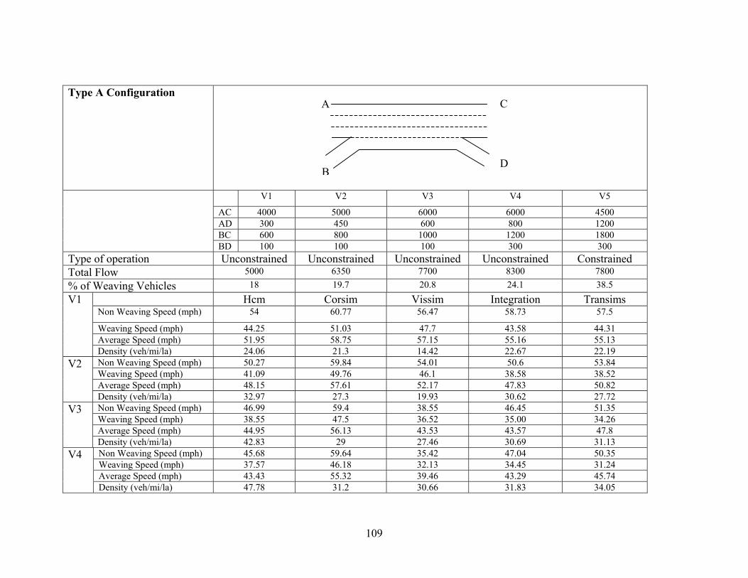
Type A Configuration

V1 V2 V3 V4 V5

AC 4000 5000 6000 6000 4500AD 300 450 600 800 1200BC 600 800 1000 1200 1800

BD 100 100 100 300 300Type of operation Unconstrained Unconstrained Unconstrained Unconstrained ConstrainedTotal Flow 5000 6350 7700 8300 7800% of Weaving Vehicles 18 19.7 20.8 24.1 38.5

Hcm Corsim Vissim Integration Transims Non Weaving Speed (mph) 54 60.77 56.47 58.73 57.5

Weaving Speed (mph) 44.25 51.03 47.7 43.58 44.31 Average Speed (mph) 51.95 58.75 57.15 55.16 55.13

V1

Density (veh/mi/la) 24.06 21.3 14.42 22.67 22.19 Non Weaving Speed (mph) 50.27 59.84 54.01 50.6 53.84 Weaving Speed (mph) 41.09 49.76 46.1 38.58 38.52 Average Speed (mph) 48.15 57.61 52.17 47.83 50.82

V2

Density (veh/mi/la) 32.97 27.3 19.93 30.62 27.72 Non Weaving Speed (mph) 46.99 59.4 38.55 46.45 51.35 Weaving Speed (mph) 38.55 47.5 36.52 35.00 34.26 Average Speed (mph) 44.95 56.13 43.53 43.57 47.8

V3

Density (veh/mi/la) 42.83 29 27.46 30.69 31.13 Non Weaving Speed (mph) 45.68 59.64 35.42 47.04 50.35 Weaving Speed (mph) 37.57 46.18 32.13 34.45 31.24 Average Speed (mph) 43.43 55.32 39.46 43.29 45.74

V4

Density (veh/mi/la) 47.78 31.2 30.66 31.83 34.05

D

CA

B

109

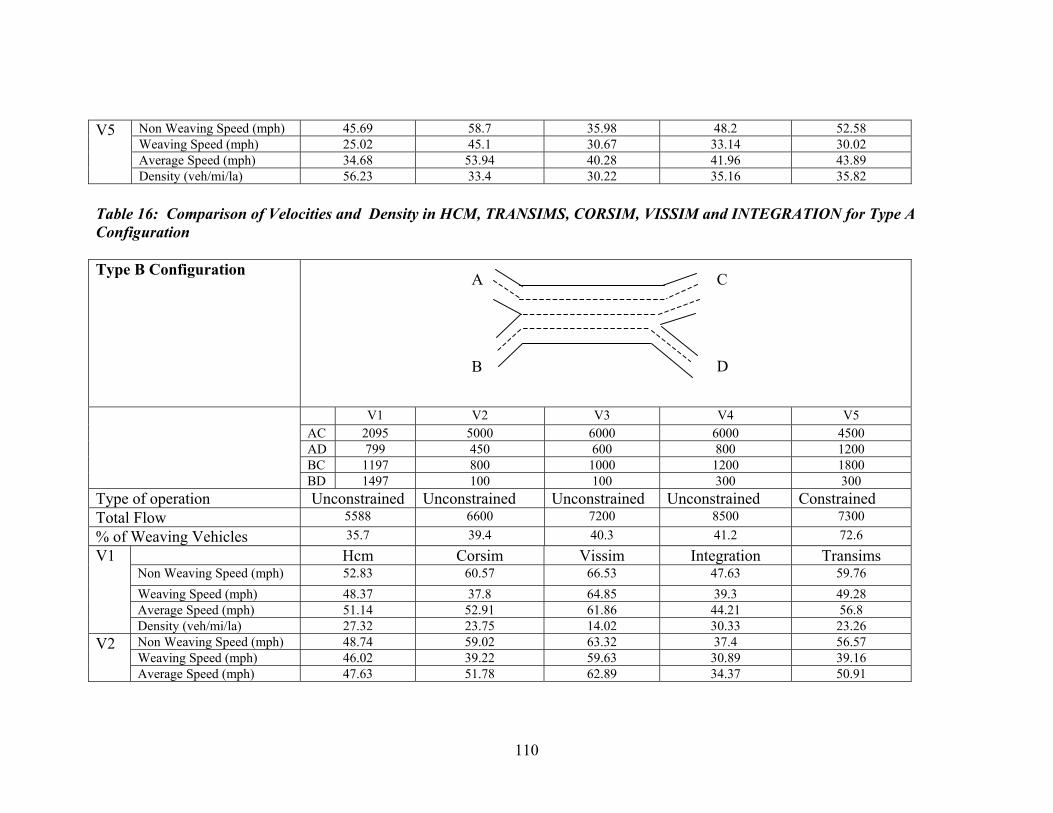
Non Weaving Speed (mph) 45.69 58.7 35.98 48.2 52.58 Weaving Speed (mph) 25.02 45.1 30.67 33.14 30.02 Average Speed (mph) 34.68 53.94 40.28 41.96 43.89

V5

Density (veh/mi/la) 56.23 33.4 30.22 35.16 35.82

Table 16: Comparison of Velocities and Density in HCM, TRANSIMS, CORSIM, VISSIM and INTEGRATION for Type A Configuration Type B Configuration

V1 V2 V3 V4 V5AC 2095 5000 6000 6000 4500AD 799 450 600 800 1200BC 1197 800 1000 1200 1800

BD 1497 100 100 300 300Type of operation Unconstrained Unconstrained Unconstrained Unconstrained ConstrainedTotal Flow 5588 6600 7200 8500 7300% of Weaving Vehicles 35.7 39.4 40.3 41.2 72.6

Hcm Corsim Vissim Integration Transims Non Weaving Speed (mph) 52.83 60.57 66.53 47.63 59.76 Weaving Speed (mph) 48.37 37.8 64.85 39.3 49.28 Average Speed (mph) 51.14 52.91 61.86 44.21 56.8

V1

Density (veh/mi/la) 27.32 23.75 14.02 30.33 23.26 Non Weaving Speed (mph) 48.74 59.02 63.32 37.4 56.57 Weaving Speed (mph) 46.02 39.22 59.63 30.89 39.16

V2

Average Speed (mph) 47.63 51.78 62.89 34.37 50.91

A C

B D

110

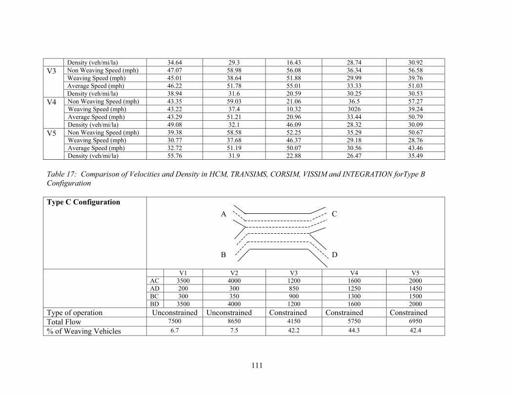
111

Density (veh/mi/la) 34.64 29.3 16.43 28.74 30.92 Non Weaving Speed (mph) 47.07 58.98 56.08 36.34 56.58 Weaving Speed (mph) 45.01 38.64 51.88 29.99 39.76 Average Speed (mph) 46.22 51.78 55.01 33.33 51.03

V3

Density (veh/mi/la) 38.94 31.6 20.59 30.25 30.53 Non Weaving Speed (mph) 43.35 59.03 21.06 36.5 57.27 Weaving Speed (mph) 43.22 37.4 10.32 3026 39.24 Average Speed (mph) 43.29 51.21 20.96 33.44 50.79

V4

Density (veh/mi/la) 49.08 32.1 46.09 28.32 30.09 Non Weaving Speed (mph) 39.38 58.58 52.25 35.29 50.67 Weaving Speed (mph) 30.77 37.68 46.37 29.18 28.76 Average Speed (mph) 32.72 51.19 50.07 30.56 43.46

V5

Density (veh/mi/la) 55.76 31.9 22.88 26.47 35.49

Table 17: Comparison of Velocities and Density in HCM, TRANSIMS, CORSIM, VISSIM and INTEGRATION forType B Configuration Type C Configuration

V1 V2 V3 V4 V5AC 3500 4000 1200 1600 2000AD 200 300 850 1250 1450BC 300 350 900 1300 1500

BD 3500 4000 1200 1600 2000Type of operation Unconstrained Unconstrained Constrained Constrained ConstrainedTotal Flow 7500 8650 4150 5750 6950% of Weaving Vehicles 6.7 7.5 42.2 44.3 42.4

A C

B D

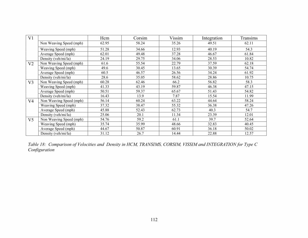
Hcm Corsim Vissim Integration TransimsNon Weaving Speed (mph) 62.95 58.24 35.26 49.51 62.11 Weaving Speed (mph) 51.28 34.66 12.93 40.19 54.3 Average Speed (mph) 62.01 49.48 37.28 46.67 61.84

V1

Density (veh/mi/la) 24.19 29.75 34.06 28.53 10.82 Non Weaving Speed (mph) 61.6 55.54 22.79 37.59 62.18 Weaving Speed (mph) 49.6 30.45 13.65 30.39 54.74 Average Speed (mph) 60.5 46.57 26.56 34.24 61.92

V2

Density (veh/mi/la) 28.6 35.05 58.62 28.86 10.75 Non Weaving Speed (mph) 60.28 62.46 66.2 56.82 58.3 Weaving Speed (mph) 41.33 43.19 59.87 46.38 47.15 Average Speed (mph) 50.51 59.37 65.67 51.43 54.82

V3

Density (veh/mi/la) 16.43 13.9 7.87 15.54 11.99 Non Weaving Speed (mph) 56.14 60.24 63.22 44.64 58.24 Weaving Speed (mph) 37.32 38.47 55.32 36.38 47.26 Average Speed (mph) 45.88 52.43 62.73 40.3 54.7

V4

Density (veh/mi/la) 25.06 20.1 11.34 23.39 12.01 Non Weaving Speed (mph) 54.76 59.2 61.1 39.7 52.64 Weaving Speed (mph) 35.74 35.99 48.66 32.83 40.45 Average Speed (mph) 44.67 50.87 60.91 36.18 50.02

V5

Density (veh/mi/la) 31.12 26.7 14.44 22.88 12.57

Table 18: Comparison of Velocities and Density in HCM, TRANSIMS, CORSIM, VISSIM and INTEGRATION for Type C Configuration

112

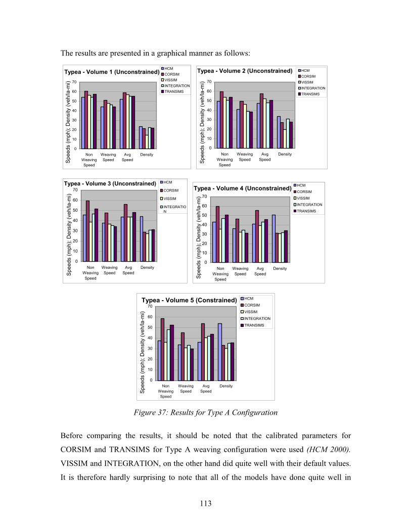
The results are presented in a graphical manner as follows:

Typea - Volume 1 (Unconstrained)

0

10

20

30

40

50

60

70

NonWeavingSpeed

WeavingSpeed

AvgSpeed

Density

HCMCORSIMVISSIMINTEGRATIONTRANSIMS

Spee

ds (m

ph);

Den

sity

(veh

/la-m

i)Typea - Volume 2 (Unconstrained)

0

10

20

30

40

50

60

70

NonWeavingSpeed

WeavingSpeed

AvgSpeed

Density

Spee

ds (m

ph);

Den

sity

(veh

/la-m

i)

HCMCORSIMVISSIMINTEGRATIONTRANSIMS

Typea - Volume 3 (Unconstrained)

0

10

20

30

40

50

60

70

NonWeavingSpeed

WeavingSpeed

AvgSpeed

Density

Spee

ds (m

ph);

Den

sity

(veh

/la-m

i)

HCM

CORSIM

VISSIM

INTEGRATION

Typea - Volume 4 (Unconstrained)

0

10

20

30

40

50

60

70

NonWeavingSpeed

WeavingSpeed

AvgSpeed

Density

Spee

ds (m

ph);

Den

sity

(veh

/la-m

i)

HCM

CORSIM

VISSIM

INTEGRATION

TRANSIMS

Typea - Volume 5 (Constrained)

0

10

20

30

40

50

60

70

NonWeavingSpeed

WeavingSpeed

AvgSpeed

Density

Spee

ds (m

ph);

Den

sity

(veh

/la-m

i)

HCM

CORSIM

VISSIM

INTEGRATION

TRANSIMS

Figure 37: Results for Type A Configuration

Before comparing the results, it should be noted that the calibrated parameters for

CORSIM and TRANSIMS for Type A weaving configuration were used (HCM 2000).

VISSIM and INTEGRATION, on the other hand did quite well with their default values.

It is therefore hardly surprising to note that all of the models have done quite well in

113

comparison to HCM and with each other. A key point with respect to CORSIM is its

consistent prediction of higher values for both weaving and non-weaving sections. This

behavior is noticed to increase with increasing volumes on the section and as the type of

operation becomes constrained. The values predicted by other three models, VISSIM,

INTEGRATION and TRANSIMS are quite close to each other in the density predictions

and in weaving speeds. Although none of the models have separate weaving logic, they

have performed well with the weaving sections in comparison to HCM. The densities

predicted, however, for all the simulation models are lower than those obtained for HCM.

The results for Type B configuration are shown in Figure 38:

Typeb - Volume 1 (Unconstrained)

0

10

20

30

40

50

60

70

NonWeavingSpeed

WeavingSpeed

AvgSpeed

Density

Spee

ds (m

ph);

Den

sity

(veh

/la-m

i)

HCM

CORSIM

VISSIM

INTEGRATION

TRANSIMS

Typeb - Volume 2 (Unconstrained)

0

10

20

30

40

50

60

70

NonWeavingSpeed

WeavingSpeed

AvgSpeed

Density

Spee

ds (m

ph);

Den

sity

(veh

/la-m

i)

HCM

CORSIM

VISSIM

INTEGRATION

TRANSIMS

Typeb - Volume 3 (Unconstrained)

0

10

20

30

40

50

60

70

NonWeavingSpeed

WeavingSpeed

AvgSpeed

DensitySpee

ds (m

ph);

Den

sity

(veh

/la-m

i)

HCM

CORSIM

VISSIM

INTEGRATION

TRANSIMS

Typeb - Volume 4 (Unconstrained)

0

10

20

30

40

50

60

70

NonWeavingSpeed

WeavingSpeed

AvgSpeed

Density

Spee

ds (m

ph);

Den

sity

(veh

/la-m

i)

HCM

CORSIM

VISSIM

INTEGRATION

TRANSIMS

114

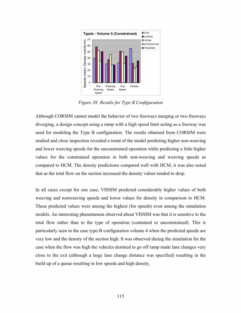
Typeb - Volume 5 (Constrained)

0

10

20

30

40

50

60

70

NonWeavingSpeed

WeavingSpeed

AvgSpeed

DensitySpee

ds (m

ph);

Den

sity

(veh

/la-m

i)

HCM

CORSIM

VISSIM

INTEGRATION

TRANSIMS

Figure 38: Results for Type B Configuration

Although CORSIM cannot model the behavior of two freeways merging or two freeways

diverging, a design concept using a ramp with a high speed limit acting as a freeway was

used for modeling the Type B configuration. The results obtained from CORSIM were

studied and close inspection revealed a trend of the model predicting higher non-weaving

and lower weaving speeds for the unconstrained operation while predicting a little higher

values for the constrained operation in both non-weaving and weaving speeds as

compared to HCM. The density predictions compared well with HCM, it was also noted

that as the total flow on the section increased the density values tended to drop.

In all cases except for one case, VISSIM predicted considerably higher values of both

weaving and nonweaving speeds and lower values for density in comparison to HCM.

These predicted values were among the highest (for speeds) even among the simulation

models. An interesting phenomenon observed about VISSIM was that it is sensitive to the

total flow rather than to the type of operation (contained or unconstrained). This is

particularly seen in the case type-B configuration volume 4 when the predicted speeds are

very low and the density of the section high. It was observed during the simulation for the

case when the flow was high the vehicles destined to go off ramp made lane changes very

close to the exit (although a large lane change distance was specified) resulting in the

build up of a queue resulting in low speeds and high density.

115

Unlike the other simulation models, INTEGRATION under predicted the weaving and

non-weaving speeds in comparison to HCM for all of the Type-B weaving section

scenarios. It is also interesting to note that the predictions for constrained type were

closer to HCM than for unconstrained flow. INTEGRATION was fairly consistent in

capturing the changes shown by HCM i.e., on increase in volumes the changes in the

speeds predicted by HCM and INTEGRATION were same. Another observation about

INTEGRATION just like HCM is the fact that the model did not show great differences

between weaving and non-weaving speeds in this configuration type B.

TRANSIMS probably fares the best in comparison to all the other simulation models

discussed considering all the cases. Although the model predicts higher non-weaving

speeds, the weaving speeds predicted are lower than those of HCM but very close. The

density values observed are also the closest to HCM and comparable to other models.

The biggest difference between HCM and TRANSIMS happens to be the difference in

the weaving and non-weaving speeds as predicted by the two. HCM for the scenarios

presented does not show a considerable difference in the weaving and the non-weaving

speeds however TRANSIMS predicts a larger difference between the two. A possible

reason for this behavior may be the handling of speeds in the model, as vehicles travel at

speeds that are multiples of 7.5 m/sec. It is also seen during the simulation that some

weaving vehicles stop for a second or two trying to lane change to get into the

appropriate lane. This behavior may also bring about the large difference in the weaving

and non-weaving speeds.

116

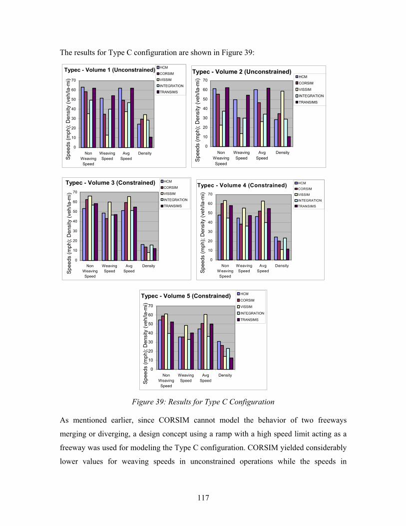
The results for Type C configuration are shown in Figure 39:

Typec - Volume 1 (Unconstrained)

0

10

20

30

40

50

60

70

NonWeavingSpeed

WeavingSpeed

AvgSpeed

Density

Spee

ds (m

ph);

Den

sity

(veh

/la-m

i)HCM

CORSIM

VISSIM

INTEGRATION

TRANSIMS

Typec - Volume 2 (Unconstrained)

0

10

20

30

40

50

60

70

NonWeavingSpeed

WeavingSpeed

AvgSpeed

Density

Spee

ds (m

ph);

Den

sity

(veh

/la-m

i) HCM

CORSIM

VISSIM

INTEGRATION

TRANSIMS

Typec - Volume 3 (Constrained)

0

10

20

30

40

50

60

70

NonWeavingSpeed

WeavingSpeed

AvgSpeed

Density

Spee

ds (m

ph);

Den

sity

(veh

/la-m

i)

HCM

CORSIM

VISSIM

INTEGRATION

TRANSIMS

Typec - Volume 4 (Constrained)

0

10

20

30

40

50

60

70

NonWeavingSpeed

WeavingSpeed

AvgSpeed

Density

Spee

ds (m

ph);

Den

sity

(veh

/la-m

i)

HCM

CORSIM

VISSIM

INTEGRATION

TRANSIMS

Typec - Volume 5 (Constrained)

0

10

20

30

40

50

60

70

NonWeavingSpeed

WeavingSpeed

AvgSpeed

Density

Spee

ds (m

ph);

Den

sity

(veh

/la-m

i)

HCM

CORSIM

VISSIM

INTEGRATION

TRANSIMS

Figure 39: Results for Type C Configuration

As mentioned earlier, since CORSIM cannot model the behavior of two freeways

merging or diverging, a design concept using a ramp with a high speed limit acting as a

freeway was used for modeling the Type C configuration. CORSIM yielded considerably

lower values for weaving speeds in unconstrained operations while the speeds in

117

constrained operations compared fairly well with HCM. The non-weaving speeds in both

cases (constrained and unconstrained) were fairly close to those predicted by HCM, the

values being slightly lower for unconstrained and higher for constrained. The density

values obtained were higher than those predicted by HCM for unconstrained operations

while for constrained operations the density values were lower. It was also observed that

the density values were closest to HCM probably second only to INTEGRATION.

Even for the Type C configuration VISSIM showed the same behavior as in Type B that

is of weaving and non-weaving speeds dropping down drastically and the density values

rising sharply for higher flows. For flows that are not very high the weaving and non-

weaving velocities were both a little higher than HCM but nonetheless comparable. The

densities corresponding to these flows were although considerably lower than those

predicted by HCM.

Probably the best model to replicate the density values close to HCM is INTEGRATION,

which yielded values close to HCM in both constrained and unconstrained operations.

The weaving and non-weaving speeds however are not tallying well for high flows or for

sections operating at their capacity. Both the velocity and the density predictions were

close to HCM for constrained type of operations for flows that were not very high.

TRANSIMS compared very well with HCM even for Type C configuration by giving the

speeds, which are much similar to HCM, but the densities obtained were much lower than

those of HCM.

118

Chapter 5 : Conclusions and Recommendations

5.1 Conclusions There have been a lot of studies involving simulation models and their applications in

various transportation operations. However the performance of these models considering

the critical maneuvers of the vehicles in particular sections of the roadways called the

weaving sections is a concern as they are the most critical regions to be modeled by any

simulation software. Hence the weaving sections involving intense lane changing

maneuvers are considered for study here.

The fundamental difference between HCM and the simulation models TRANSIMS,

CORSIM, VISSIM and INTEGRATION is that HCM is a deterministic model in which

the results are based on traditional data collected while the other models are stochastic

simulation models, which can model results based on several driver behavior parameters.

A 30-minute simulation run for all the models only represents one point of the data

sample while HCM may represent an average value of samples. Although a series of

simulation runs were performed for every configuration and an average collected for all

the models, it only reduces the average error and gets the results closer to the true

convergence value of the simulation.

The objective of the research was to carry out a comparative analysis of the models so as

to be able to judge the performance of the models. In the course of the analysis the

following conclusions were drawn.

119

CORSIM did not compare well with HCM probably because of the fact that it cannot

model the behavior of two freeways merging or two freeways diverging, the way in

which the Type B and Type C configurations are modeled. It yielded lower values of

speeds for unconstrained operations and a little higher value of speeds for constrained

operations.

VISSIM predicted higher values of speeds and lower values of densities. The model

proved to be sensitive to the total flows rather than the type of operation (constrained

or unconstrained). The model did not show a behavior consistent with HCM.

Although INTEGRATION performed well for the Type A and Type B configurations

it did not do well with sections operating at high flows for unconstrained operations.

But it was especially good in predicting the densities and fairly accurate with speeds.

Overall it can be concluded that it performed well with the weaving sections with

respect to HCM.

TRANSIMS gave good results in comparison to all the other models discussed. The

model predicted the speeds and densities very close to HCM although densities did

not compare very well with HCM for the Type C configuration. A major difference

between HCM and TRANSIMS proved to be the difference in the weaving and non-

weaving speeds as predicted by the two. HCM did not show a considerable difference

in the weaving and the non-weaving speeds however TRANSIMS showed a greater

difference between the two. This kind of behavior can be attributed to the ‘cellular

automata’ kind of simulation used by TRANSIMS Microsimulator. Even though

TRANSIMS did not give a wide range of microscopic characteristics that can be

changed such as driver characteristics, the effect had been brought out by properly

adjusting the parameters provided by the model.

5.2 Recommendations

The following recommendations are suggested to the models:

120

In TRANSIMS, the vehicles when considering a lane change should consider the

speeds of the lead and the following car in the adjacent lane into which the vehicle is

trying to do a lane change. TRANSIMS considers a lane changing movement when

the gap backward is more than 5 cells irrespective of the speeds of the vehicle. This is

not true in the real life scenario. Also the vehicles are considered to have a fixed

length. TRANSIMS follows same logic for simulating freeways and arterials, which

may not replicate the real life scenario when simulating either of them.

In CORSIM when the vehicles are trying to merger on to freeway from on ramp they

immediately get into the lane adjacent to the auxiliary lane within 100 ft of the gore

area, which is very unlikely in the real life. The merging logic could be altered to

make a realistic behavior possible.

VISSIM is not able to perform lane changes in the weaving sections realistically.

Vehicles start to do a lane change within 100 ft of the gore area at the exit ramp trying

to exit the freeway, which results in queue formation throughout the section. There is

no anticipatory lane changing logic, which disables the user to input the percentage of

vehicles yielding to the entering traffic.

HCM does not consider the various driver characteristics, which play an important

role while evaluating the weaving speeds of the vehicles. And also it gives out an

approximated weaving speed of the vehicles in a section rather than considering the

varying speeds of the vehicles in that section.

121

Bibliography

“CORSIM User Manual”, FHWA , Contract No. DTFH1-92-Z-00074, 1996

Catherine C. McGhee, “Evaluation of methods for Freeway Operational Analysis”,

Virginia Transportation Research Council in Cooperation with U.S Department of

Transportation, Federal Highway Administration, October 2001.

Drew D. (1968), Traffic Flow Theory and Control, McGraw Hill. New York. Fellendorf, M., and Vortisch, P., “Validation of the Microscopic Traffic Flow Model

VISSIM in Different Real-World Situations”, prepared at Karlsruhe, Geramny.

Garber, Nicholas J. And Gadiraju, Ravi, "Factors affecting Speed Variance and Its

Influence on Accidents" Transportation Research Record No. 1213, pp 64-71.

Halati, A., et al., “Lane changing in Freeway Simulation models,” Transportation

Research Board Publication, 1990

Halati, A., Lieu, H., and Walker, S., “ CORSIM – Corridor Traffic Simulation

Model”, Transportation Research Board, 76th Annual Meeting, Washington D.C.

“Highway Capacity Manual, Special Report 209 ”, Transportation Research Board,

Washington, D. C., 1997.

Hobeika, A., “A Course Manual on TRANSIMS” published at Virginia Tech used as

notes for course CEE 5644.

Jillella S., Hobeika A., “A Comparitive Study of Weaving Sections in TRANSIMS

and Highway Capacity Manual”, Masters Thesis, Virginia Polytechnic Institute and

State University, June 2001.

122

May A.D. (1990), Traffic Flow Fundamentals, Prentice Hall, Englewood Cliffs, New

Jersey.

Moen, B., Fitts, J., Carter, D., and Quyang, Y., “ A Comparison of the VISSIM

Model to other widely used Traffic Simulation and Analysis Programs” prepared at

Karlsruhe, Germany.

Nagel, K. et al, “TRANSIMS traffic flow characteristics”, LA-UR 97-3531, Los

Alamos Unclassified Report, Los Alamos National Laboratory, Los Alamos, NM,

USA.

Nagel, K. et al, “Two Lane traffic rules for cellular Automata: A systematic

approach”, LA-UR 97-4706, Los Alamos Unclassified Report, Los Alamos National

Laboratory, Los Alamos, NM, USA.

Nagel, K., “Particle Hopping Models and Traffic Flow Theory”, LA-UR 95-2908,

Los Alamos Unclassified Report, Los Alamos National Laboratory, Los Alamos,

NM, USA.

Owen L, Zhang Y, Rao L, and McHale G., “Traffic Flow Simulation Using

CORSIM”, Proceedings of the 2000 Winter Simulation Conference.

Prevedouros P, and Wang Y., “Simulation of a Large Freeway/Arterial Network with

CORSIM, INTEGRATION and WATSim”, Transportation Research Board, 78th

Annual Meeting, January 10-15, 1999, Washington, D.C.

Rakha H., and Crowther B., “ A Comparison of the Greenshields, Pipes, and Van

Aerde Car-Following and Traffic Stream Models” Virginia Polytechnic Institute and

State University.

123

Rakha, H., and Crowther, B. (2000), “A Comparison and Calibration of the

INTEGRATION and CORSIM Steady-State Car-Following Behavior”,Virginia

Polytechnic Institute and State University.

Ramachandran S., Hobeika A., “Analysis of freeway weaving areas under corridor

simulator and Highway Capacity Manual”, Masters Thesis, Virginia Polytechnic

Institute and State University, November 1997.

Van Aerde, M., & Associates. (2000) Windows User's Guide – Volume I and II:

Fundamental Model Features and Advanced Model Features, Kingston, Ontario.

Van Aerde, M., Rakha, H. (1999), “Microsimulation of Traffic With and Without

Adaptive Cruise Control: Model Logic”, Paper Submitted to ITS America.

VISSIM user Manual, Developed at PTV Planung Transport Verkehr AG.

White T., “General Overview of Simulation Models”, Compendium of Technical

Papers, 49th Annual Meeting, Southern District Institute of Transportation Engineers,

April 22-25, 2001.

124

APPENDIX A

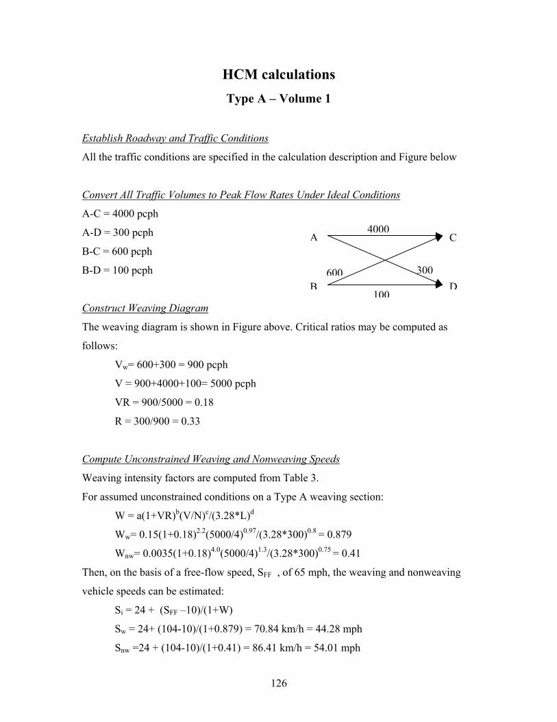
HCM calculations Type A – Volume 1

Establish Roadway and Traffic Conditions

All the traffic conditions are specified in the calculation description and Figure below

Convert All Traffic Volumes to Peak Flow Rates Under Ideal Conditions

A-C = 4000 pcph

A

B

C

D600 300

4000

100

A-D = 300 pcph

B-C = 600 pcph

B-D = 100 pcph

Construct Weaving Diagram

The weaving diagram is shown in Figure above. Critical ratios may be computed as

follows:

Vw= 600+300 = 900 pcph

V = 900+4000+100= 5000 pcph

VR = 900/5000 = 0.18

R = 300/900 = 0.33

Compute Unconstrained Weaving and Nonweaving Speeds

Weaving intensity factors are computed from Table 3.

For assumed unconstrained conditions on a Type A weaving section:

W = a(1+VR)b(V/N)c/(3.28*L)d

Ww= 0.15(1+0.18)2.2(5000/4)0.97/(3.28*300)0.8 = 0.879

Wnw= 0.0035(1+0.18)4.0(5000/4)1.3/(3.28*300)0.75 = 0.41

Then, on the basis of a free-flow speed, SFF , of 65 mph, the weaving and nonweaving

vehicle speeds can be estimated:

Si = 24 + (SFF –10)/(1+W)

Sw = 24+ (104-10)/(1+0.879) = 70.84 km/h = 44.28 mph

Snw =24 + (104-10)/(1+0.41) = 86.41 km/h = 54.01 mph

126

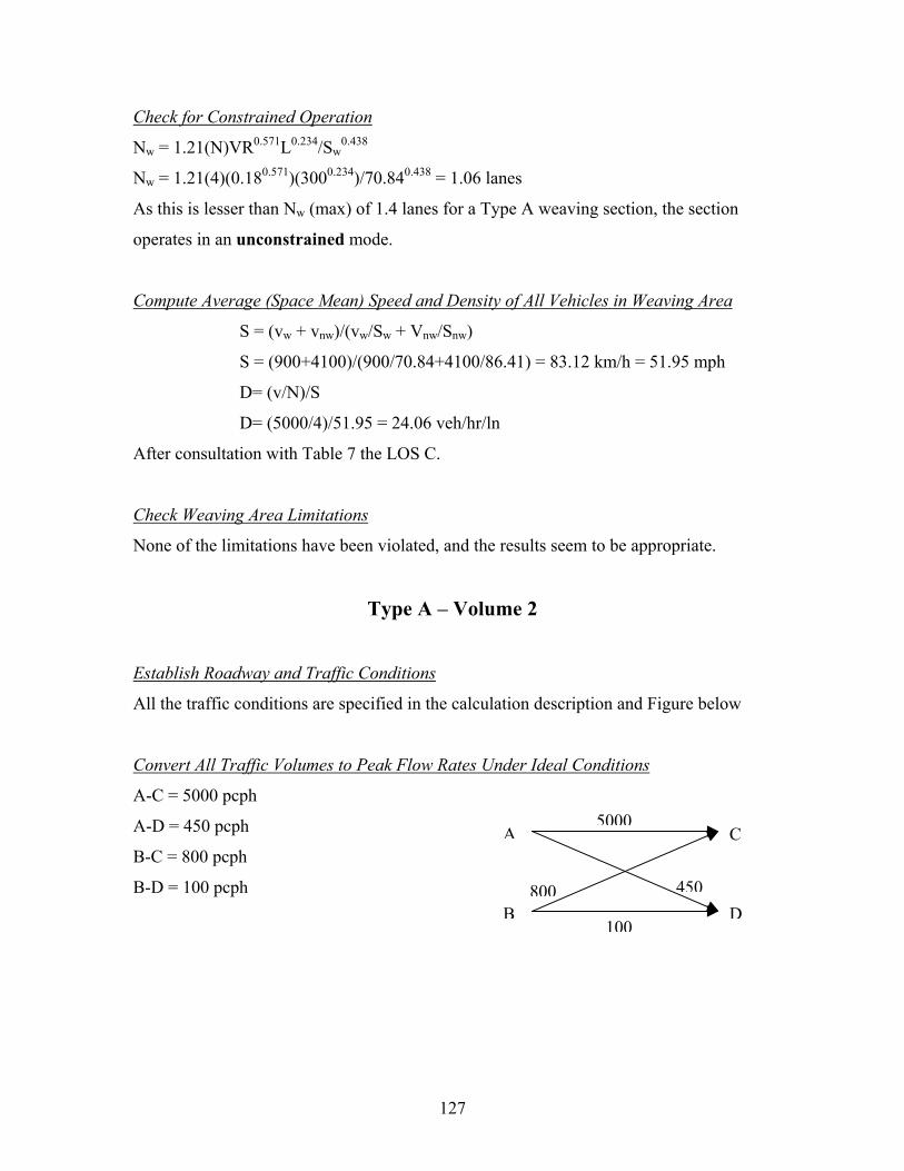
Check for Constrained Operation

Nw = 1.21(N)VR0.571L0.234/Sw0.438

Nw = 1.21(4)(0.180.571)(3000.234)/70.840.438 = 1.06 lanes

As this is lesser than Nw (max) of 1.4 lanes for a Type A weaving section, the section

operates in an unconstrained mode.

Compute Average (Space Mean) Speed and Density of All Vehicles in Weaving Area

S = (vw + vnw)/(vw/Sw + Vnw/Snw)

S = (900+4100)/(900/70.84+4100/86.41) = 83.12 km/h = 51.95 mph

D= (v/N)/S

D= (5000/4)/51.95 = 24.06 veh/hr/ln

After consultation with Table 7 the LOS C.

Check Weaving Area Limitations

None of the limitations have been violated, and the results seem to be appropriate.

Type A – Volume 2

Establish Roadway and Traffic Conditions

All the traffic conditions are specified in the calculation description and Figure below

Convert All Traffic Volumes to Peak Flow Rates Under Ideal Conditions

A-C = 5000 pcph

A

B

C

D800 450

5000

100

A-D = 450 pcph

B-C = 800 pcph

B-D = 100 pcph

127

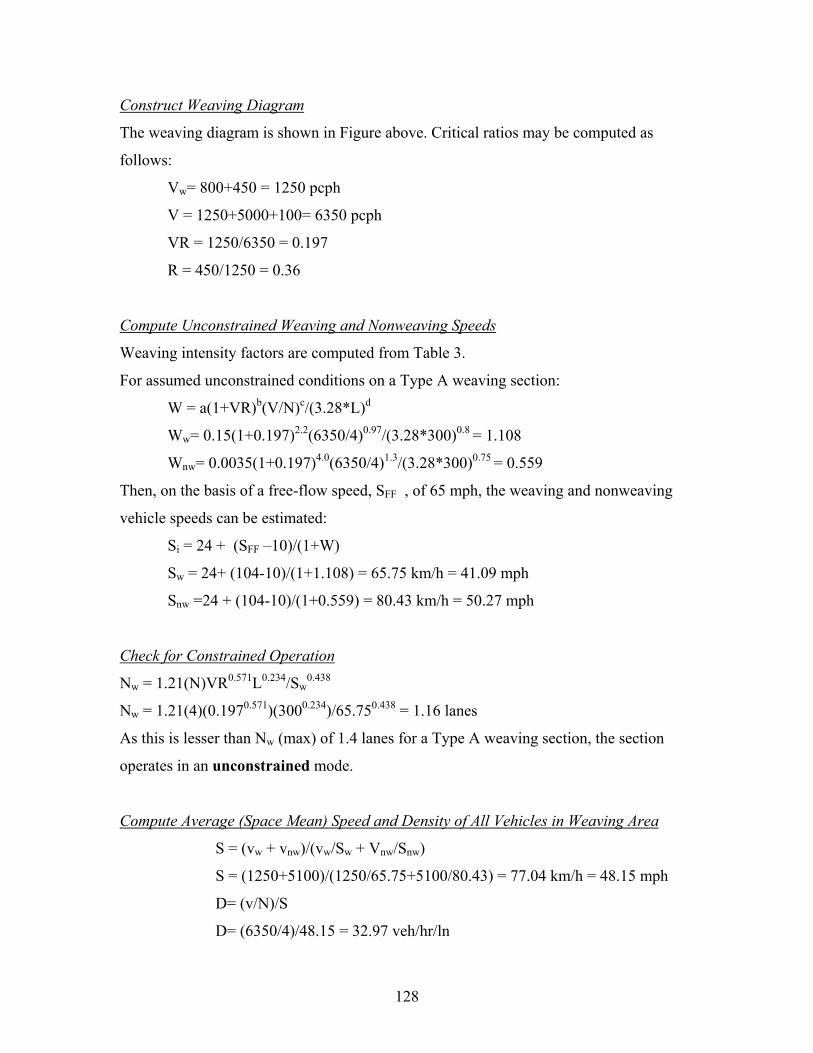
Construct Weaving Diagram

The weaving diagram is shown in Figure above. Critical ratios may be computed as

follows:

Vw= 800+450 = 1250 pcph

V = 1250+5000+100= 6350 pcph

VR = 1250/6350 = 0.197

R = 450/1250 = 0.36

Compute Unconstrained Weaving and Nonweaving Speeds

Weaving intensity factors are computed from Table 3.

For assumed unconstrained conditions on a Type A weaving section:

W = a(1+VR)b(V/N)c/(3.28*L)d

Ww= 0.15(1+0.197)2.2(6350/4)0.97/(3.28*300)0.8 = 1.108

Wnw= 0.0035(1+0.197)4.0(6350/4)1.3/(3.28*300)0.75 = 0.559

Then, on the basis of a free-flow speed, SFF , of 65 mph, the weaving and nonweaving

vehicle speeds can be estimated:

Si = 24 + (SFF –10)/(1+W)

Sw = 24+ (104-10)/(1+1.108) = 65.75 km/h = 41.09 mph

Snw =24 + (104-10)/(1+0.559) = 80.43 km/h = 50.27 mph

Check for Constrained Operation

Nw = 1.21(N)VR0.571L0.234/Sw0.438

Nw = 1.21(4)(0.1970.571)(3000.234)/65.750.438 = 1.16 lanes

As this is lesser than Nw (max) of 1.4 lanes for a Type A weaving section, the section

operates in an unconstrained mode.

Compute Average (Space Mean) Speed and Density of All Vehicles in Weaving Area

S = (vw + vnw)/(vw/Sw + Vnw/Snw)

S = (1250+5100)/(1250/65.75+5100/80.43) = 77.04 km/h = 48.15 mph

D= (v/N)/S

D= (6350/4)/48.15 = 32.97 veh/hr/ln

128

After consultation with Table 7 the LOS D.

Check Weaving Area Limitations

None of the limitations have been violated, and the results seem to be appropriate.

Type A – Volume 3

Establish Roadway and Traffic Conditions

All the traffic conditions are specified in the calculation description and Figure below

Convert All Traffic Volumes to Peak Flow Rates Under Ideal Conditions

A-C = 6000 pcph

A

B

C

D1000 600

6000

100

A-D = 600 pcph

B-C = 1000 pcph

B-D = 100 pcph

Construct Weaving Diagram

The weaving diagram is shown in Figure above. Critical ratios may be computed as

follows:

Vw= 1000+600 = 1600 pcph

V = 1600+6000+100= 7700 pcph

VR = 1600/7700 = 0.208

R = 600/1600 = 0.375

Compute Unconstrained Weaving and Nonweaving Speeds

Weaving intensity factors are computed from Table 3.

For assumed unconstrained conditions on a Type A weaving section:

W = a(1+VR)b(V/N)c/(3.28*L)d

Ww= 0.15(1+0.208)2.2(7700/4)0.97/(3.28*300)0.8 = 1.336

Wnw= 0.0035(1+0.208)4.0(7700/4)1.3/(3.28*300)0.75 = 0.719

129

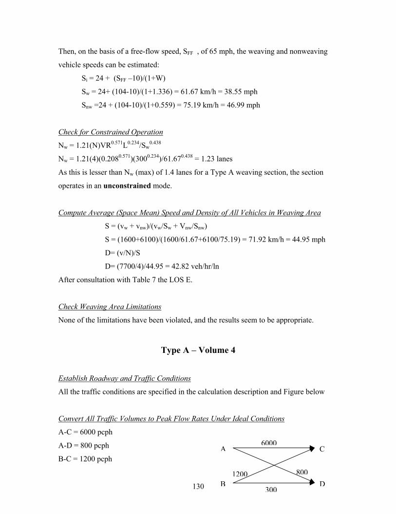
Then, on the basis of a free-flow speed, SFF , of 65 mph, the weaving and nonweaving

vehicle speeds can be estimated:

Si = 24 + (SFF –10)/(1+W)

Sw = 24+ (104-10)/(1+1.336) = 61.67 km/h = 38.55 mph

Snw =24 + (104-10)/(1+0.559) = 75.19 km/h = 46.99 mph

Check for Constrained Operation

Nw = 1.21(N)VR0.571L0.234/Sw0.438

Nw = 1.21(4)(0.2080.571)(3000.234)/61.670.438 = 1.23 lanes

As this is lesser than Nw (max) of 1.4 lanes for a Type A weaving section, the section

operates in an unconstrained mode.

Compute Average (Space Mean) Speed and Density of All Vehicles in Weaving Area

S = (vw + vnw)/(vw/Sw + Vnw/Snw)

S = (1600+6100)/(1600/61.67+6100/75.19) = 71.92 km/h = 44.95 mph

D= (v/N)/S

D= (7700/4)/44.95 = 42.82 veh/hr/ln

After consultation with Table 7 the LOS E.

Check Weaving Area Limitations

None of the limitations have been violated, and the results seem to be appropriate.

Type A – Volume 4

Establish Roadway and Traffic Conditions

All the traffic conditions are specified in the calculation description and Figure below

Convert All Traffic Volumes to Peak Flow Rates Under Ideal Conditions

A-C = 6000 pcph

A

B

C

D1200 800

6000

300

A-D = 800 pcph

B-C = 1200 pcph

130

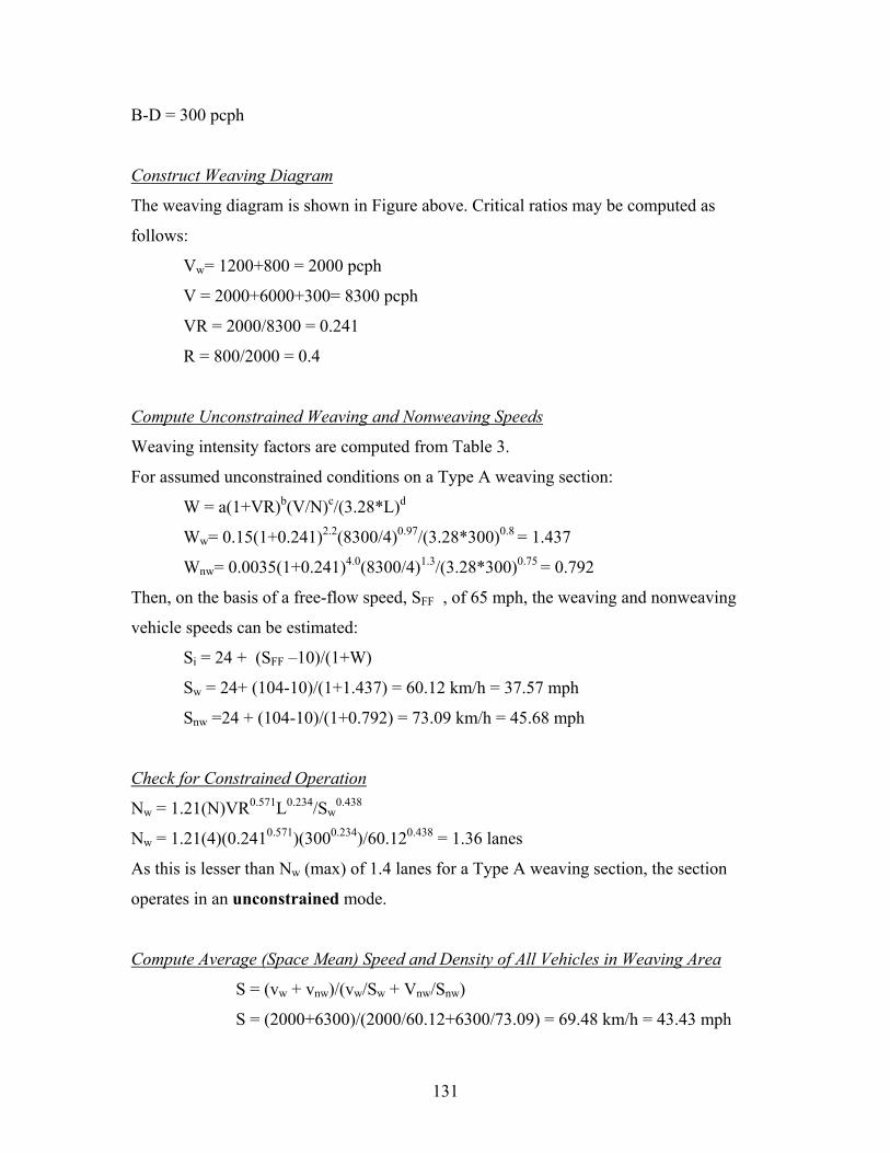
B-D = 300 pcph

Construct Weaving Diagram

The weaving diagram is shown in Figure above. Critical ratios may be computed as

follows:

Vw= 1200+800 = 2000 pcph

V = 2000+6000+300= 8300 pcph

VR = 2000/8300 = 0.241

R = 800/2000 = 0.4

Compute Unconstrained Weaving and Nonweaving Speeds

Weaving intensity factors are computed from Table 3.

For assumed unconstrained conditions on a Type A weaving section:

W = a(1+VR)b(V/N)c/(3.28*L)d

Ww= 0.15(1+0.241)2.2(8300/4)0.97/(3.28*300)0.8 = 1.437

Wnw= 0.0035(1+0.241)4.0(8300/4)1.3/(3.28*300)0.75 = 0.792

Then, on the basis of a free-flow speed, SFF , of 65 mph, the weaving and nonweaving

vehicle speeds can be estimated:

Si = 24 + (SFF –10)/(1+W)

Sw = 24+ (104-10)/(1+1.437) = 60.12 km/h = 37.57 mph

Snw =24 + (104-10)/(1+0.792) = 73.09 km/h = 45.68 mph

Check for Constrained Operation

Nw = 1.21(N)VR0.571L0.234/Sw0.438

Nw = 1.21(4)(0.2410.571)(3000.234)/60.120.438 = 1.36 lanes

As this is lesser than Nw (max) of 1.4 lanes for a Type A weaving section, the section

operates in an unconstrained mode.

Compute Average (Space Mean) Speed and Density of All Vehicles in Weaving Area

S = (vw + vnw)/(vw/Sw + Vnw/Snw)

S = (2000+6300)/(2000/60.12+6300/73.09) = 69.48 km/h = 43.43 mph

131

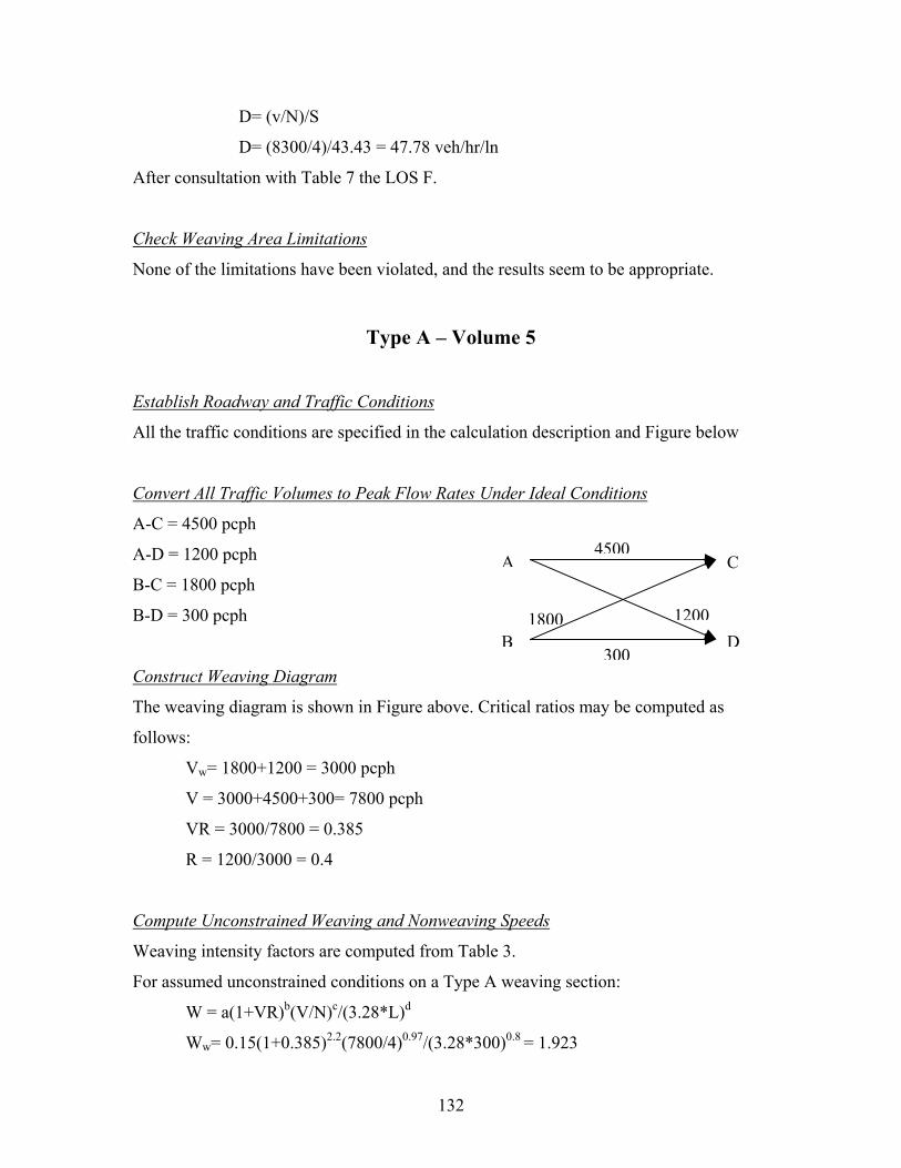
D= (v/N)/S

D= (8300/4)/43.43 = 47.78 veh/hr/ln

After consultation with Table 7 the LOS F.

Check Weaving Area Limitations

None of the limitations have been violated, and the results seem to be appropriate.

Type A – Volume 5

Establish Roadway and Traffic Conditions

All the traffic conditions are specified in the calculation description and Figure below

Convert All Traffic Volumes to Peak Flow Rates Under Ideal Conditions

A-C = 4500 pcph

A

B

C

D1800 1200

4500

300

A-D = 1200 pcph

B-C = 1800 pcph

B-D = 300 pcph

Construct Weaving Diagram

The weaving diagram is shown in Figure above. Critical ratios may be computed as

follows:

Vw= 1800+1200 = 3000 pcph

V = 3000+4500+300= 7800 pcph

VR = 3000/7800 = 0.385

R = 1200/3000 = 0.4

Compute Unconstrained Weaving and Nonweaving Speeds

Weaving intensity factors are computed from Table 3.

For assumed unconstrained conditions on a Type A weaving section:

W = a(1+VR)b(V/N)c/(3.28*L)d

Ww= 0.15(1+0.385)2.2(7800/4)0.97/(3.28*300)0.8 = 1.923

132

Wnw= 0.0035(1+0.385)4.0(7800/4)1.3/(3.28*300)0.75 = 1.386

Then, on the basis of a free-flow speed, SFF , of 65 mph, the weaving and nonweaving

vehicle speeds can be estimated:

Si = 24 + (SFF –10)/(1+W)

Sw = 24+ (104-10)/(1+1.923) = 54.11 km/h = 33.82 mph

Snw =24 + (104-10)/(1+1.386) = 60.89 km/h = 38.05 mph

Check for Constrained Operation

Nw = 1.21(N)VR0.571L0.234/Sw0.438

Nw = 1.21(4)(0.3850.571)(3000.234)/54.110.438 = 1.855 lanes

As this is greater than Nw (max) of 1.4 lanes for a Type A weaving section, the section

operates in a constrained mode.

Repeat the step for constrained Weaving and Nonweaving Speeds

Weaving intensity factors are computed from Table 3.

For constrained conditions on a Type A weaving section:

Ww= 0.35(1+0.385)2.2(7800/4)0.97/(3.28*300)0.8 = 4.487

Wnw= 0.002(1+0.385)4.0(7800/4)1.3/(3.28*300)0.75 = 0.792

Then, on the basis of a free-flow speed, SFF , of 65 mph, the weaving and nonweaving

vehicle speeds can be estimated:

Si = 24 + (SFF –10)/(1+W)

Sw = 24+ (104-10)/(1+4.487) = 40.04 km/h = 25.02 mph

Snw =24 + (104-10)/(1+1.386) = 73.11 km/h = 45.69 mph

Compute Average (Space Mean) Speed and Density of All Vehicles in Weaving Area

S = (vw + vnw)/(vw/Sw + Vnw/Snw)

S = (3000+4800)/(3000/40.04+4800/73.11) = 55.48 km/h = 34.68 mph

D= (v/N)/S

D= (8300/4)/34.68 = 56.23 veh/hr/ln

After consultation with Table 7 the LOS F.

133

Check Weaving Area Limitations

None of the limitations have been violated, and the results seem to be appropriate.

Type B – Volume 1

Establish Roadway and Traffic Conditions

All the traffic conditions are specified in the calculation description and Figure below

Convert All Traffic Volumes to Peak Flow Rates Under Ideal Conditions

CA-C = 2095 pcph

A-D = 799 pcph

B-C = 1197 pcph

B-D = 1497 pcph

Construct Weaving Diagram

The weaving diagram is shown in Figures above. C

follows:

Vw= 1197 + 799 = 1996 pcph

V = 1197 + 2095 + 1497 = 5588 pcph

VR = 1996 / 5588 = 0.357

R = 799 / 1996 = 0.400

Compute Unconstrained Weaving and Nonweaving

Weaving intensity factors are computed from Table

For assumed unconstrained conditions on a Type B

( )d

cb

i LNvVRa

W28.3

)1(

+

=

134

A

B

ritical ratios may be computed a

Speeds

5.

weaving section:

D

1197 799

2095

1497

s

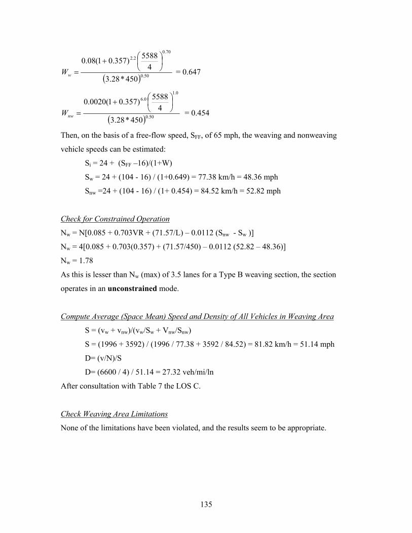
( ) 50.0

70.02.2

450*28.34

5588)357.01(08.0

+

=wW = 0.647

( ) 50.0

0.10.6

450*28.34

5588)357.01(0020.0

+

=nwW = 0.454

Then, on the basis of a free-flow speed, SFF, of 65 mph, the weaving and nonweaving

vehicle speeds can be estimated:

Si = 24 + (SFF –16)/(1+W)

Sw = 24 + (104 - 16) / (1+0.649) = 77.38 km/h = 48.36 mph

Snw =24 + (104 - 16) / (1+ 0.454) = 84.52 km/h = 52.82 mph

Check for Constrained Operation

Nw = N[0.085 + 0.703VR + (71.57/L) – 0.0112 (Snw - Sw )]

Nw = 4[0.085 + 0.703(0.357) + (71.57/450) – 0.0112 (52.82 – 48.36)]

Nw = 1.78

As this is lesser than Nw (max) of 3.5 lanes for a Type B weaving section, the section

operates in an unconstrained mode.

Compute Average (Space Mean) Speed and Density of All Vehicles in Weaving Area

S = (vw + vnw)/(vw/Sw + Vnw/Snw)

S = (1996 + 3592) / (1996 / 77.38 + 3592 / 84.52) = 81.82 km/h = 51.14 mph

D= (v/N)/S

D= (6600 / 4) / 51.14 = 27.32 veh/mi/ln

After consultation with Table 7 the LOS C.

Check Weaving Area Limitations

None of the limitations have been violated, and the results seem to be appropriate.

135

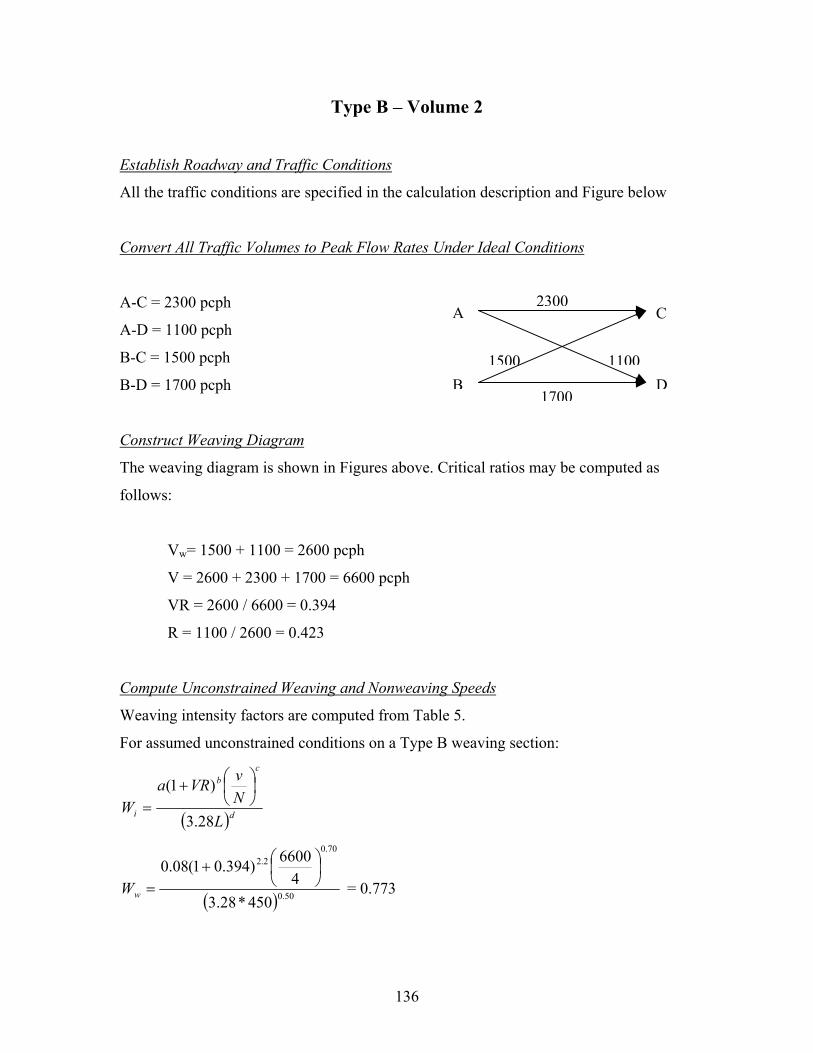
Type B – Volume 2

Establish Roadway and Traffic Conditions

All the traffic conditions are specified in the calculation description and Figure below

Convert All Traffic Volumes to Peak Flow Rates Under Ideal Conditions

A-C = 2300 pcph CA

B1500 1100

2300

1700

A-D = 1100 pcph

B-C = 1500 pcph

B-D = 1700 pcph

Construct Weaving Diagram

The weaving diagram is shown in Figures above. Critical ratios may be computed a

follows:

Vw= 1500 + 1100 = 2600 pcph

V = 2600 + 2300 + 1700 = 6600 pcph

VR = 2600 / 6600 = 0.394

R = 1100 / 2600 = 0.423

Compute Unconstrained Weaving and Nonweaving Speeds

Weaving intensity factors are computed from Table 5.

For assumed unconstrained conditions on a Type B weaving section:

( )d

cb

i LNvVRa

W28.3

)1(

+

=

( ) 50.0

70.02.2

450*28.34

6600)394.01(08.0

+

=wW = 0.773

136

D

s

( ) 50.0

0.10.6

450*28.34

6600)394.01(0020.0

+

=nwW = 0.63

Then, on the basis of a free-flow speed, SFF, of 65 mph, the weaving and non-weaving

vehicle speeds can be estimated:

Si = 24 + (SFF –16)/(1+W)

Sw = 24 + (104 - 16) / (1+0.773) = 73.64 km/h = 46.02 mph

Snw =24 + (104 - 16) / (1+ 0.63) = 77.98 km/h = 48.74 mph

Check for Constrained Operation

Nw = N[0.085 + 0.703VR + (71.57/L) – 0.0112 (Snw - Sw )]

Nw = 4[0.085 + 0.703(0.394) + (71.57/450) – 0.0112 (48.74 – 46.02)]

Nw = 1.96

As this is lesser than Nw (max) of 3.5 lanes for a Type B weaving section, the section

operates in an unconstrained mode.

Compute Average (Space Mean) Speed and Density of All Vehicles in Weaving Area

S = (vw + vnw)/(vw/Sw + Vnw/Snw)

S = (2600 + 4000) / (2600 / 73.64 + 4000 / 77.98) = 76.21 km/h = 47.63 mph

D= (v/N)/S

D= (6600 / 4) / 47.63 = 34.64 veh/mi/ln

After consultation with Table 7 the LOS D.

Check Weaving Area Limitations

None of the limitations have been violated, and the results seem to be appropriate.

Type B – Volume 3

Establish Roadway and Traffic Conditions

All the traffic conditions are specified in the calculation description and Figure below

137

Convert All Traffic Volumes to Peak Flow Rates Under Ideal Conditions

A-C = 2500 pcph A

B

C

D1700 1200

2500

1800

A-D = 1200 pcph

B-C = 1700 pcph

B-D = 1800 pcph

Construct Weaving Diagram

The weaving diagram is shown in Figures above. Critical ratios may be computed as

follows:

Vw= 1500 + 1100 = 2600 pcph

V = 2600 + 2300 + 1700 = 6600 pcph

VR = 2600 / 6600 = 0.394

R = 1100 / 2600 = 0.423

Compute Unconstrained Weaving and Nonweaving Speeds

Weaving intensity factors are computed from Table 5.

For assumed unconstrained conditions on a Type B weaving section:

( )d

cb

i LNvVRa

W28.3

)1(

+

=

( ) 50.0

70.02.2

450*28.34

7200)403.01(08.0

+

=wW = 0.833

( ) 50.0

0.10.6

450*28.34

7200)403.01(0020.0

+

=nwW = 0.714

Then, on the basis of a free-flow speed, SFF , of 65 mph, the weaving and nonweaving

vehicle speeds can be estimated:

Si = 24 + (SFF –16)/(1+W)

138

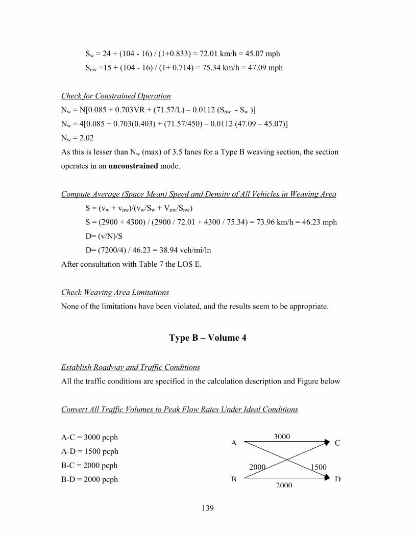
Sw = 24 + (104 - 16) / (1+0.833) = 72.01 km/h = 45.07 mph

Snw =15 + (104 - 16) / (1+ 0.714) = 75.34 km/h = 47.09 mph

Check for Constrained Operation

Nw = N[0.085 + 0.703VR + (71.57/L) – 0.0112 (Snw - Sw )]

Nw = 4[0.085 + 0.703(0.403) + (71.57/450) – 0.0112 (47.09 – 45.07)]

Nw = 2.02

As this is lesser than Nw (max) of 3.5 lanes for a Type B weaving section, the section

operates in an unconstrained mode.

Compute Average (Space Mean) Speed and Density of All Vehicles in Weaving Area

S = (vw + vnw)/(vw/Sw + Vnw/Snw)

S = (2900 + 4300) / (2900 / 72.01 + 4300 / 75.34) = 73.96 km/h = 46.23 mph

D= (v/N)/S

D= (7200/4) / 46.23 = 38.94 veh/mi/ln

After consultation with Table 7 the LOS E.

Check Weaving Area Limitations

None of the limitations have been violated, and the results seem to be appropriate.

Type B – Volume 4

Establish Roadway and Traffic Conditions

All the traffic conditions are specified in the calculation description and Figure below

Convert All Traffic Volumes to Peak Flow Rates Under Ideal Conditions

A-C = 3000 pcph

A-D = 1500 pcph

B-C = 2000 pcph

B-D = 2000 pcph B

A C

D2000 1500

3000

2000

139

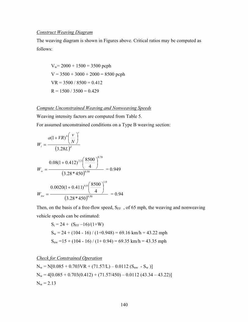
Construct Weaving Diagram

The weaving diagram is shown in Figures above. Critical ratios may be computed as

follows:

Vw= 2000 + 1500 = 3500 pcph

V = 3500 + 3000 + 2000 = 8500 pcph

VR = 3500 / 8500 = 0.412

R = 1500 / 3500 = 0.429

Compute Unconstrained Weaving and Nonweaving Speeds

Weaving intensity factors are computed from Table 5.

For assumed unconstrained conditions on a Type B weaving section:

( )d

cb

i LNvVRa

W28.3

)1(

+

=

( ) 50.0

70.02.2

450*28.34

8500)412.01(08.0

+

=wW = 0.949

( ) 50.0

0.10.6

450*28.34

8500)411.01(0020.0

+

=nwW = 0.94

Then, on the basis of a free-flow speed, SFF , of 65 mph, the weaving and nonweaving

vehicle speeds can be estimated:

Si = 24 + (SFF –16)/(1+W)

Sw = 24 + (104 - 16) / (1+0.948) = 69.16 km/h = 43.22 mph

Snw =15 + (104 - 16) / (1+ 0.94) = 69.35 km/h = 43.35 mph

Check for Constrained Operation

Nw = N[0.085 + 0.703VR + (71.57/L) – 0.0112 (Snw - Sw )]

Nw = 4[0.085 + 0.703(0.412) + (71.57/450) – 0.0112 (43.34 – 43.22)]

Nw = 2.13

140

As this is lesser than Nw (max) of 3.5 lanes for a Type B weaving section, the section

operates in an unconstrained mode.

Compute Average (Space Mean) Speed and Density of All Vehicles in Weaving Area

S = (vw + vnw)/(vw/Sw + Vnw/Snw)

S = (3500 + 5000) / (3500 / 69.16 + 5000 / 69.35) = 69.27 km/h = 43.29 mph

D= (v/N)/S

D= (5588 / 4) / 43.29 = 49.08 veh/mi/ln

After consultation with Table 7 the LOS F.

Check Weaving Area Limitations

None of the limitations have been violated, and the results seem to be appropriate.

Type B – Volume 5

Establish Roadway and Traffic Conditions

All the traffic conditions are specified in the calculation description and Figure below

Convert All Traffic Volumes to Peak Flow Rates Under Ideal Conditions

A-C = 1000 pcph

A-D = 2800 pcph A

B

C

D2500 2800

1000

1000

B-C = 2500 pcph

B-D = 1000 pcph

Construct Weaving Diagram

The weaving diagram is shown in Figures above. Critical ratios may be computed as

follows:

Vw= 2500 + 2800 = 5300 pcph

V = 5300 + 1000 + 1000 = 7300 pcph

VR = 5300 / 7300 = 0.726

R = 2800 / 5300 = 0.528

141

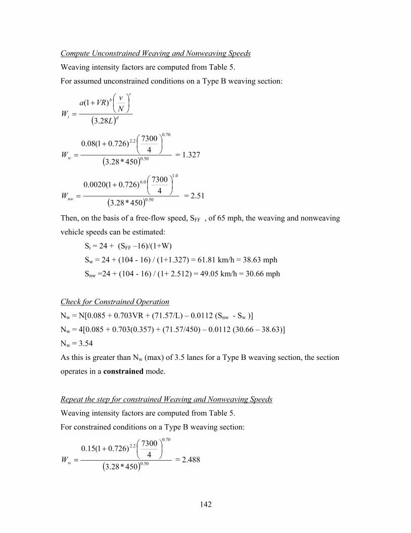
Compute Unconstrained Weaving and Nonweaving Speeds

Weaving intensity factors are computed from Table 5.

For assumed unconstrained conditions on a Type B weaving section:

( )d

cb

i LNvVRa

W28.3

)1(

+

=

( ) 50.0

70.02.2

450*28.34

7300)726.01(08.0

+

=wW = 1.327

( ) 50.0

0.10.6

450*28.34

7300)726.01(0020.0

+

=nwW = 2.51

Then, on the basis of a free-flow speed, SFF , of 65 mph, the weaving and nonweaving

vehicle speeds can be estimated:

Si = 24 + (SFF –16)/(1+W)

Sw = 24 + (104 - 16) / (1+1.327) = 61.81 km/h = 38.63 mph

Snw =24 + (104 - 16) / (1+ 2.512) = 49.05 km/h = 30.66 mph

Check for Constrained Operation

Nw = N[0.085 + 0.703VR + (71.57/L) – 0.0112 (Snw - Sw )]

Nw = 4[0.085 + 0.703(0.357) + (71.57/450) – 0.0112 (30.66 – 38.63)]

Nw = 3.54

As this is greater than Nw (max) of 3.5 lanes for a Type B weaving section, the section

operates in a constrained mode.

Repeat the step for constrained Weaving and Nonweaving Speeds

Weaving intensity factors are computed from Table 5.

For constrained conditions on a Type B weaving section:

( ) 50.0

70.02.2

450*28.34

7300)726.01(15.0

+

=wW = 2.488

142

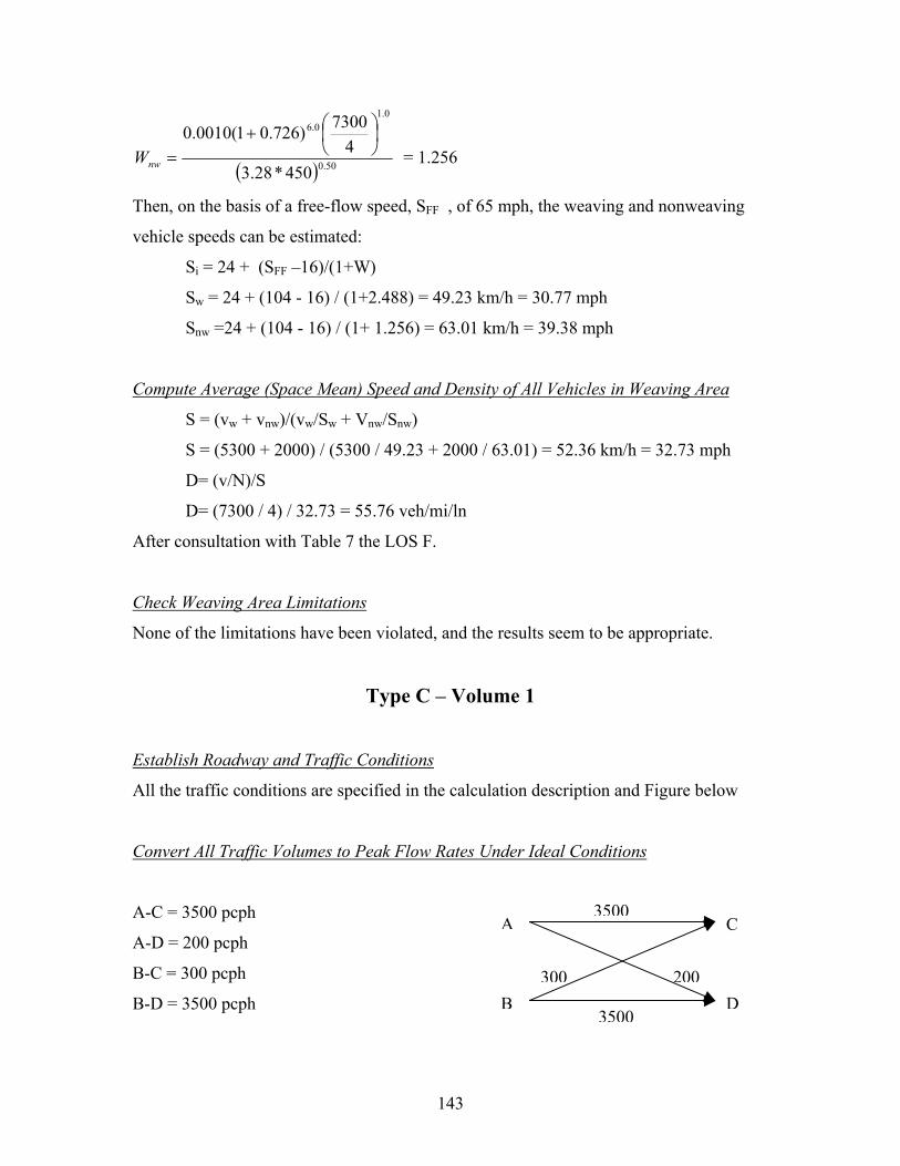
( ) 50.0

0.10.6

450*28.34

7300)726.01(0010.0

+

=nwW = 1.256

Then, on the basis of a free-flow speed, SFF , of 65 mph, the weaving and nonweaving

vehicle speeds can be estimated:

Si = 24 + (SFF –16)/(1+W)

Sw = 24 + (104 - 16) / (1+2.488) = 49.23 km/h = 30.77 mph

Snw =24 + (104 - 16) / (1+ 1.256) = 63.01 km/h = 39.38 mph

Compute Average (Space Mean) Speed and Density of All Vehicles in Weaving Area

S = (vw + vnw)/(vw/Sw + Vnw/Snw)

S = (5300 + 2000) / (5300 / 49.23 + 2000 / 63.01) = 52.36 km/h = 32.73 mph

D= (v/N)/S

D= (7300 / 4) / 32.73 = 55.76 veh/mi/ln

After consultation with Table 7 the LOS F.

Check Weaving Area Limitations

None of the limitations have been violated, and the results seem to be appropriate.

Type C – Volume 1

Establish Roadway and Traffic Conditions

All the traffic conditions are specified in the calculation description and Figure below

Convert All Traffic Volumes to Peak Flow Rates Under Ideal Conditions

A-C = 3500 pcph A

B

C

D300 200

3500

3500

A-D = 200 pcph

B-C = 300 pcph

B-D = 3500 pcph

143

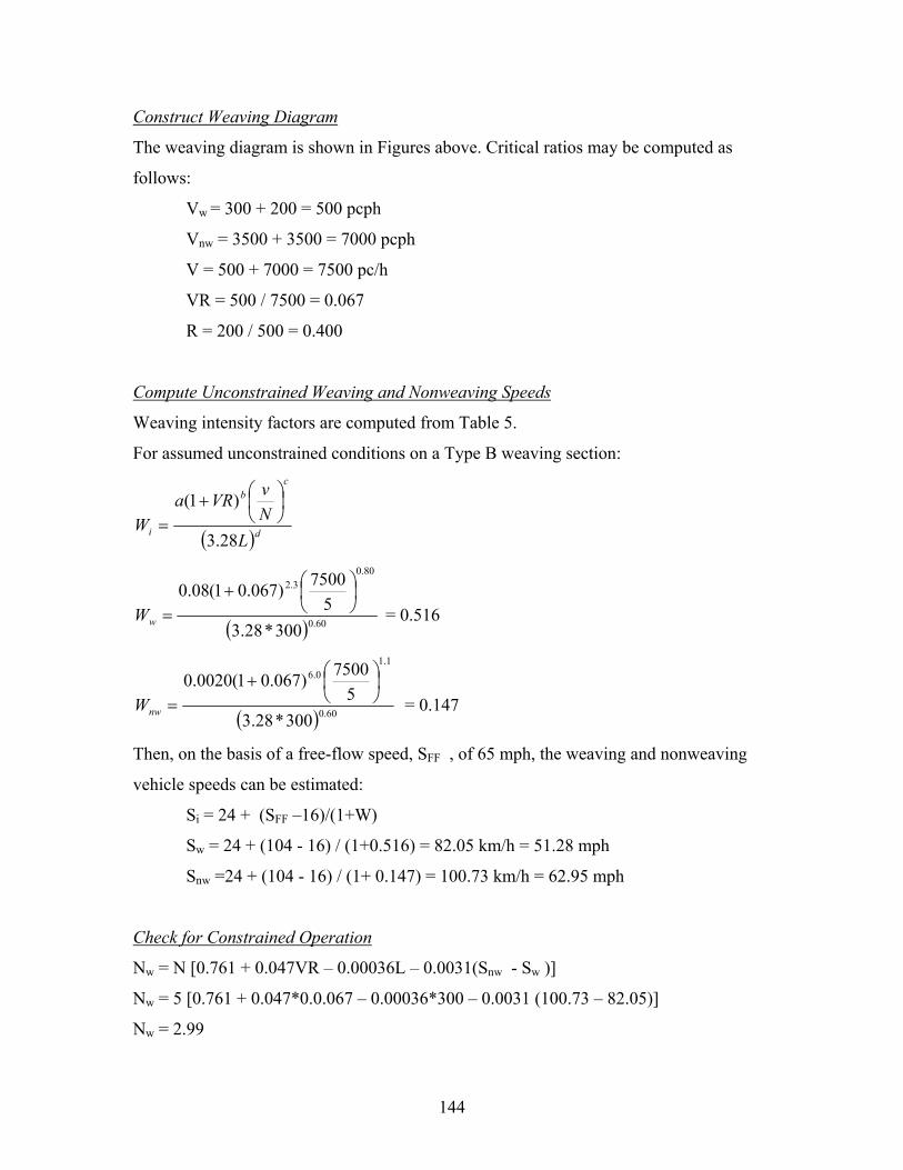
Construct Weaving Diagram

The weaving diagram is shown in Figures above. Critical ratios may be computed as

follows:

Vw = 300 + 200 = 500 pcph

Vnw = 3500 + 3500 = 7000 pcph

V = 500 + 7000 = 7500 pc/h

VR = 500 / 7500 = 0.067

R = 200 / 500 = 0.400

Compute Unconstrained Weaving and Nonweaving Speeds

Weaving intensity factors are computed from Table 5.

For assumed unconstrained conditions on a Type B weaving section:

( )d

cb

i LNvVRa

W28.3

)1(

+

=

( ) 60.0

80.03.2

300*28.35

7500)067.01(08.0

+

=wW = 0.516

( ) 60.0

1.10.6

300*28.35

7500)067.01(0020.0

+

=nwW = 0.147

Then, on the basis of a free-flow speed, SFF , of 65 mph, the weaving and nonweaving

vehicle speeds can be estimated:

Si = 24 + (SFF –16)/(1+W)

Sw = 24 + (104 - 16) / (1+0.516) = 82.05 km/h = 51.28 mph

Snw =24 + (104 - 16) / (1+ 0.147) = 100.73 km/h = 62.95 mph

Check for Constrained Operation

Nw = N [0.761 + 0.047VR – 0.00036L – 0.0031(Snw - Sw )]

Nw = 5 [0.761 + 0.047*0.0.067 – 0.00036*300 – 0.0031 (100.73 – 82.05)]

Nw = 2.99

144

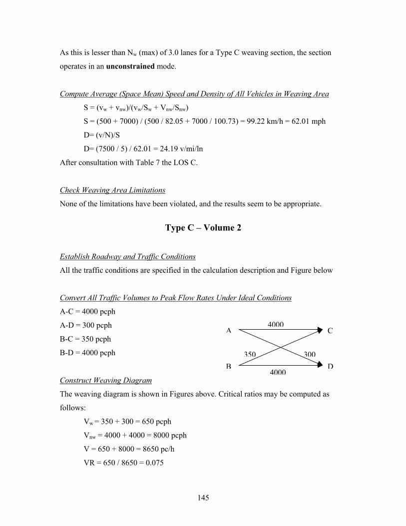
As this is lesser than Nw (max) of 3.0 lanes for a Type C weaving section, the section

operates in an unconstrained mode.

Compute Average (Space Mean) Speed and Density of All Vehicles in Weaving Area

S = (vw + vnw)/(vw/Sw + Vnw/Snw)

S = (500 + 7000) / (500 / 82.05 + 7000 / 100.73) = 99.22 km/h = 62.01 mph

D= (v/N)/S

D= (7500 / 5) / 62.01 = 24.19 v/mi/ln

After consultation with Table 7 the LOS C.

Check Weaving Area Limitations

None of the limitations have been violated, and the results seem to be appropriate.

Type C – Volume 2

Establish Roadway and Traffic Conditions

All the traffic conditions are specified in the calculation description and Figure below

Convert All Traffic Volumes to Peak Flow Rates Under Ideal Conditions

A-C = 4000 pcph

A-D = 300 pcph A

B

C

D350 300

4000

4000

B-C = 350 pcph

B-D = 4000 pcph

Construct Weaving Diagram

The weaving diagram is shown in Figures above. Critical ratios may be computed as

follows:

Vw = 350 + 300 = 650 pcph

Vnw = 4000 + 4000 = 8000 pcph

V = 650 + 8000 = 8650 pc/h

VR = 650 / 8650 = 0.075

145

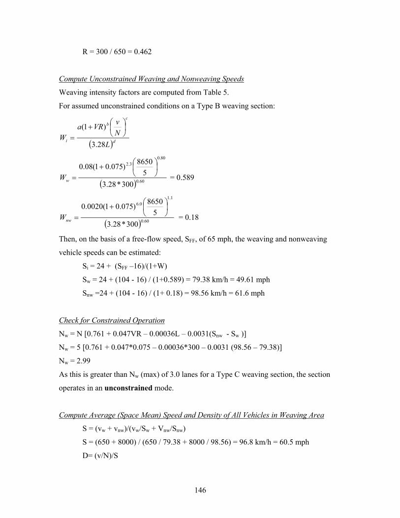
R = 300 / 650 = 0.462

Compute Unconstrained Weaving and Nonweaving Speeds

Weaving intensity factors are computed from Table 5.

For assumed unconstrained conditions on a Type B weaving section:

( )d

cb

i LNvVRa

W28.3

)1(

+

=

( ) 60.0

80.03.2

300*28.35

8650)075.01(08.0

+

=wW = 0.589

( ) 60.0

1.10.6

300*28.35

8650)075.01(0020.0

+

=nwW = 0.18

Then, on the basis of a free-flow speed, SFF, of 65 mph, the weaving and nonweaving

vehicle speeds can be estimated:

Si = 24 + (SFF –16)/(1+W)

Sw = 24 + (104 - 16) / (1+0.589) = 79.38 km/h = 49.61 mph

Snw =24 + (104 - 16) / (1+ 0.18) = 98.56 km/h = 61.6 mph

Check for Constrained Operation

Nw = N [0.761 + 0.047VR – 0.00036L – 0.0031(Snw - Sw )]

Nw = 5 [0.761 + 0.047*0.075 – 0.00036*300 – 0.0031 (98.56 – 79.38)]

Nw = 2.99

As this is greater than Nw (max) of 3.0 lanes for a Type C weaving section, the section

operates in an unconstrained mode.

Compute Average (Space Mean) Speed and Density of All Vehicles in Weaving Area

S = (vw + vnw)/(vw/Sw + Vnw/Snw)

S = (650 + 8000) / (650 / 79.38 + 8000 / 98.56) = 96.8 km/h = 60.5 mph

D= (v/N)/S

146

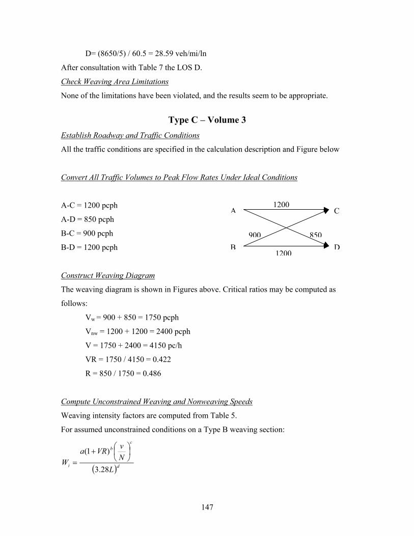
D= (8650/5) / 60.5 = 28.59 veh/mi/ln

After consultation with Table 7 the LOS D.

Check Weaving Area Limitations

None of the limitations have been violated, and the results seem to be appropriate.

Type C – Volume 3

Establish Roadway and Traffic Conditions

All the traffic conditions are specified in the calculation description and Figure below

Convert All Traffic Volumes to Peak Flow Rates Under Ideal Conditions

A-C = 1200 pcph A C

D900 850

1200

1200B

A-D = 850 pcph

B-C = 900 pcph

B-D = 1200 pcph

Construct Weaving Diagram

The weaving diagram is shown in Figures above. Critical ratios may be computed as

follows:

Vw = 900 + 850 = 1750 pcph

Vnw = 1200 + 1200 = 2400 pcph

V = 1750 + 2400 = 4150 pc/h

VR = 1750 / 4150 = 0.422

R = 850 / 1750 = 0.486

Compute Unconstrained Weaving and Nonweaving Speeds

Weaving intensity factors are computed from Table 5.

For assumed unconstrained conditions on a Type B weaving section:

( )d

cb

i LNvVRa

W28.3

)1(

+

=

147

( ) 60.0

80.03.2

300*28.35

4150)422.01(08.0

+

=wW = 0.622

( ) 60.0

1.10.6

300*28.35

4150)422.01(0020.0

+

=nwW = 0.429

Then, on the basis of a free-flow speed, SFF , of 65 mph, the weaving and nonweaving

vehicle speeds can be estimated:

Si = 24 + (SFF –16)/(1+W)

Sw = 24 + (104 - 16) / (1+0.622) = 78.24 km/h = 48.9 mph

Snw =24 + (104 - 16) / (1+ 0.429) = 85.56 km/h = 53.47 mph

Check for Constrained Operation

Nw = N [0.761 + 0.047VR – 0.00036L – 0.0031(Snw - Sw )]

Nw = 5 [0.761 + 0.047*0.424 – 0.00036*300 – 0.0031 (85.56 – 78.24)]

Nw = 3.25

As this is greater than Nw (max) of 3.0 lanes for a Type C weaving section, the section

operates in a constrained mode.

Repeat for Constrained Operation

Weaving intensity factors are computed from Table 5.

For constrained conditions on a Type C weaving section:

( ) 60.0

80.03.2

300*28.35

4150)422.01(14.0

+

=wW = 1.089

( ) 60.0

1.10.6

300*28.35

4150)422.01(001.0

+

=nwW = 0.215

Sw = 24 + (104 - 16) / (1+1.089) = 66.13 km/h = 41.33 mph

Snw = 24 + (104 - 16) / (1+ 0.215) = 96.44 km/h = 60.28 mph

148

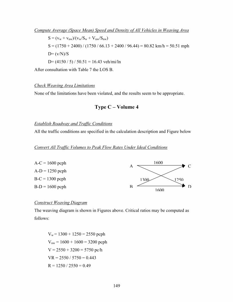
Compute Average (Space Mean) Speed and Density of All Vehicles in Weaving Area

S = (vw + vnw)/(vw/Sw + Vnw/Snw)

S = (1750 + 2400) / (1750 / 66.13 + 2400 / 96.44) = 80.82 km/h = 50.51 mph

D= (v/N)/S

D= (4150 / 5) / 50.51 = 16.43 veh/mi/ln

After consultation with Table 7 the LOS B.

Check Weaving Area Limitations

None of the limitations have been violated, and the results seem to be appropriate.

Type C – Volume 4

Establish Roadway and Traffic Conditions

All the traffic conditions are specified in the calculation description and Figure below

Convert All Traffic Volumes to Peak Flow Rates Under Ideal Conditions

A-C = 1600 pcph A

B

C

D1300 1250

1600

1600

A-D = 1250 pcph

B-C = 1300 pcph

B-D = 1600 pcph

Construct Weaving Diagram

The weaving diagram is shown in Figures above. Critical ratios may be computed as

follows:

Vw = 1300 + 1250 = 2550 pcph

Vnw = 1600 + 1600 = 3200 pcph

V = 2550 + 3200 = 5750 pc/h

VR = 2550 / 5750 = 0.443

R = 1250 / 2550 = 0.49

149

Compute Unconstrained Weaving and Nonweaving Speeds

Weaving intensity factors are computed from Table 5.

For assumed unconstrained conditions on a Type B weaving section:

( )d

cb

i LNvVRa

W28.3

)1(

+

=

( ) 60.0

80.03.2

300*28.35

5750)443.01(08.0

+

=wW = 0.837

( ) 60.0

1.10.6

300*28.35

5750)443.01(0020.0

+

=nwW = 0.674

Then, on the basis of a free-flow speed, SFF, of 65 mph, the weaving and non-weaving

vehicle speeds can be estimated:

Si = 24 + (SFF –16)/(1+W)

Sw = 24 + (104 - 16) / (1+0.837) = 71.92 km/h = 44.95 mph

Snw =24 + (104 - 16) / (1+ 0.674) = 76.58 km/h = 47.86 mph

Check for Constrained Operation

Nw = N [0.761 + 0.047VR – 0.00036L – 0.0031(Snw - Sw )]

Nw = 5 [0.761 + 0.047*0.443 – 0.00036*300 – 0.0031 (76.58 – 71.92)]

Nw = 3.29

As this is greater than Nw (max) of 3.0 lanes for a Type C weaving section, the section

operates in a constrained mode.

Repeat for Constrained Operation

Weaving intensity factors are computed from Table 5.

For constrained conditions on a Type C weaving section:

( ) 60.0

80.03.2

300*28.35

5750)443.01(14.0

+

=wW = 1.464

150

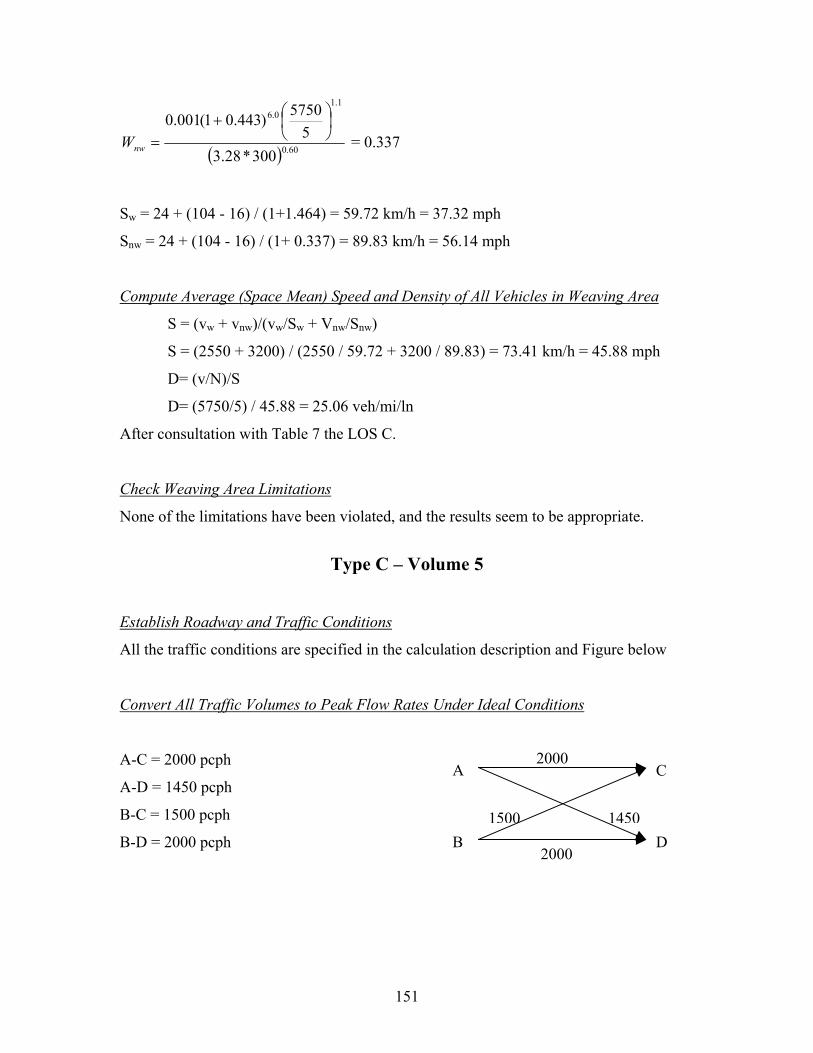
( ) 60.0

1.10.6

300*28.35

5750)443.01(001.0

+

=nwW = 0.337

Sw = 24 + (104 - 16) / (1+1.464) = 59.72 km/h = 37.32 mph

Snw = 24 + (104 - 16) / (1+ 0.337) = 89.83 km/h = 56.14 mph

Compute Average (Space Mean) Speed and Density of All Vehicles in Weaving Area

S = (vw + vnw)/(vw/Sw + Vnw/Snw)

S = (2550 + 3200) / (2550 / 59.72 + 3200 / 89.83) = 73.41 km/h = 45.88 mph

D= (v/N)/S

D= (5750/5) / 45.88 = 25.06 veh/mi/ln

After consultation with Table 7 the LOS C.

Check Weaving Area Limitations

None of the limitations have been violated, and the results seem to be appropriate.

Type C – Volume 5

Establish Roadway and Traffic Conditions

All the traffic conditions are specified in the calculation description and Figure below

Convert All Traffic Volumes to Peak Flow Rates Under Ideal Conditions

CA-C = 2000 pcph

A-D = 1450 pcph

B-C = 1500 pcph

B-D = 2000 pcph

151

A

B

D 1500 1450

2000

2000

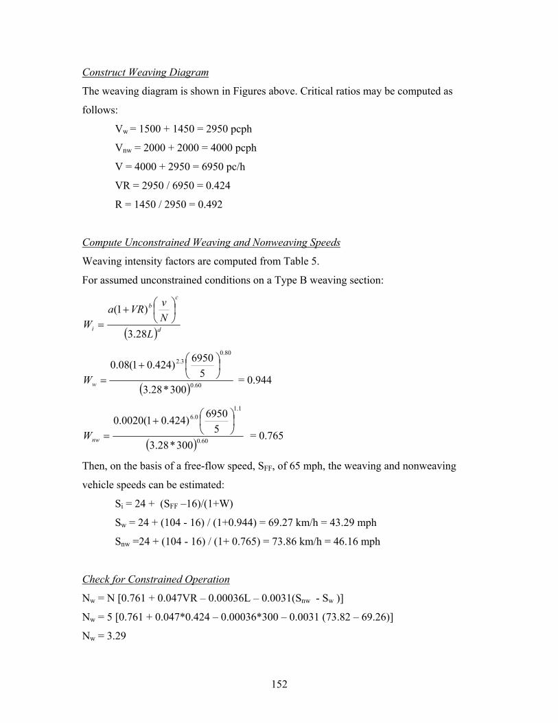
Construct Weaving Diagram

The weaving diagram is shown in Figures above. Critical ratios may be computed as

follows:

V = 1500 + 1450 = 2950 pcph w

Vnw = 2000 + 2000 = 4000 pcph

V = 4000 + 2950 = 6950 pc/h

VR = 2950 / 6950 = 0.424

R = 1450 / 2950 = 0.492

Compute Unconstrained Weaving and Nonweaving Speeds

Weaving intensity factors are computed from Table 5.

For assumed unconstrained conditions on a Type B weaving section:

( )d

cb

i LNvVRa

W28.3

)1(

+

=

( ) 60.0

80.03.2

300*28.35

6950)424.01(08.0

+

=wW = 0.944

( ) 60.0

1.10.6

300*28.35

6950)424.01(0020.0

+

=nwW = 0.765

Then, on the basis of a free-flow speed, SFF, of 65 mph, the weaving and nonweaving

vehicle speeds can be estimated:

Si = 24 + (SFF –16)/(1+W)

Sw = 24 + (104 - 16) / (1+0.944) = 69.27 km/h = 43.29 mph

Snw =24 + (104 - 16) / (1+ 0.765) = 73.86 km/h = 46.16 mph

Check for Constrained Operation

Nw = N [0.761 + 0.047VR – 0.00036L – 0.0031(Snw - Sw )]

N = 5 [0.761 + 0.047*0.424 – 0.00036*300 – 0.0031 (73.82 – 69.26)]w

Nw = 3.29

152

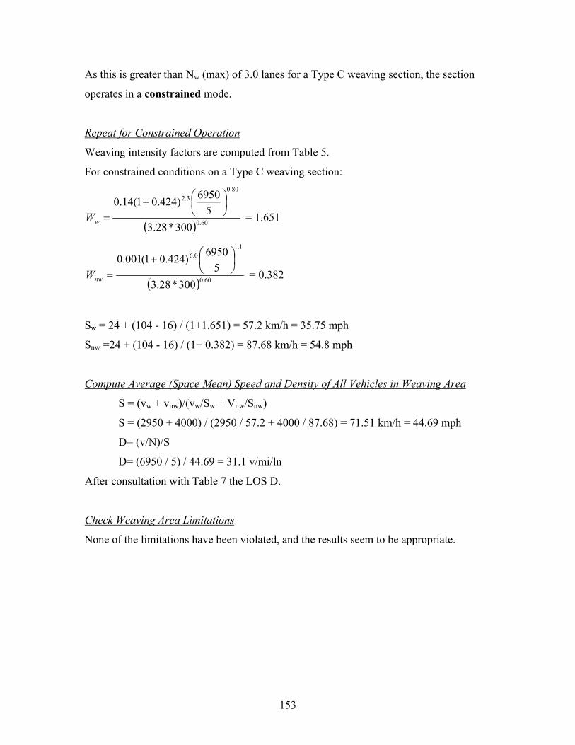
As this is greater than Nw (max) of 3.0 lanes for a Type C weaving section, the section

operates in a constrained mode.

Repeat for Constrained Operation

Weaving intensity factors are computed from Table 5.

For constrained conditions on a Type C weaving section:

( ) 60.0

80.03.2

300*28.35

6950)424.01(14.0

+

=wW = 1.651

( ) 60.0

1.10.6

300*28.35

6950)424.01(001.0

+

=nwW = 0.382

Sw = 24 + (104 - 16) / (1+1.651) = 57.2 km/h = 35.75 mph

Snw =24 + (104 - 16) / (1+ 0.382) = 87.68 km/h = 54.8 mph

Compute Average (Space Mean) Speed and Density of All Vehicles in Weaving Area

S = (vw + vnw)/(vw/Sw + Vnw/Snw)

S = (2950 + 4000) / (2950 / 57.2 + 4000 / 87.68) = 71.51 km/h = 44.69 mph

D= (v/N)/S

D= (6950 / 5) / 44.69 = 31.1 v/mi/ln

After consultation with Table 7 the LOS D.

Check Weaving Area Limitations

None of the limitations have been violated, and the results seem to be appropriate.

153

APPENDIX B

154

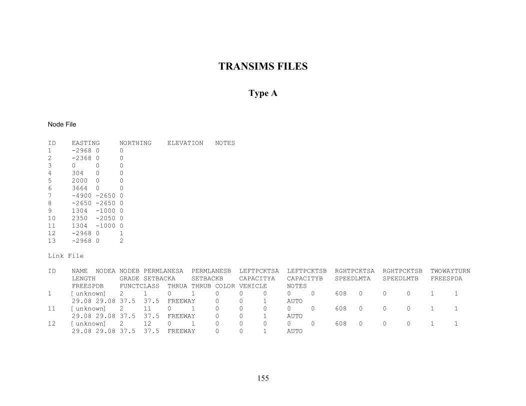
TRANSIMS FILES

Type A

Node File ID EASTING NORTHING ELEVATION NOTES 1 -2968 0 0 2 -2368 0 0 3 0 0 0 4 304 0 0 5 2000 0 0 6 3664 0 0 7 -4900 -2650 0 8 -2650 -2650 0 9 1304 -1000 0 10 2350 -2050 0 11 1304 -1000 0 12 -2968 0 1 13 -2968 0 2 Link File ID NAME NODEA NODEB PERMLANESA PERMLANESB LEFTPCKTSA LEFTPCKTSB RGHTPCKTSA RGHTPCKTSB TWOWAYTURN LENGTH GRADE SETBACKA SETBACKB CAPACITYA CAPACITYB SPEEDLMTA SPEEDLMTB FREESPDA FREESPDB FUNCTCLASS THRUA THRUB COLOR VEHICLE NOTES 1 [unknown] 2 1 0 1 0 0 0 0 0 608 0 0 0 1 1 29.08 29.08 37.5 37.5 FREEWAY 0 0 1 AUTO 11 [unknown] 2 11 0 1 0 0 0 0 0 608 0 0 0 1 1 29.08 29.08 37.5 37.5 FREEWAY 0 0 1 AUTO 12 [unknown] 2 12 0 1 0 0 0 0 0 608 0 0 0 1 1 29.08 29.08 37.5 37.5 FREEWAY 0 0 1 AUTO

155

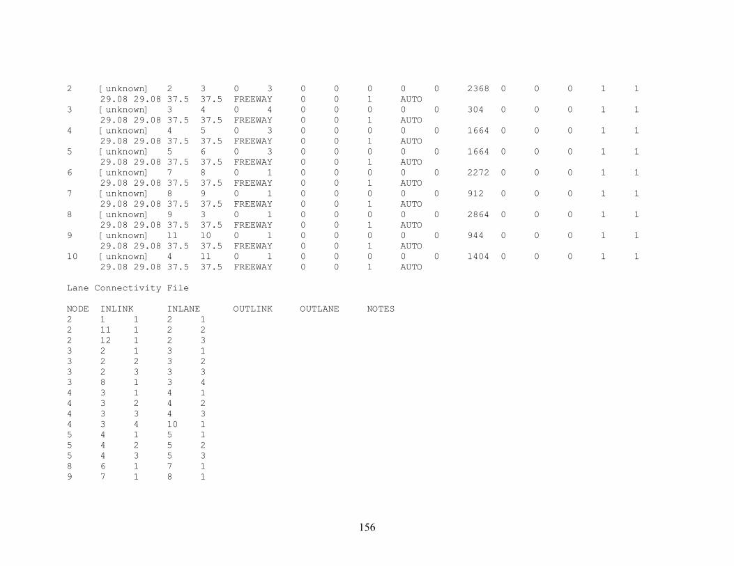
2 [unknown] 2 3 0 3 0 0 0 0 0 2368 0 0 0 1 1 29.08 29.08 37.5 37.5 FREEWAY 0 0 1 AUTO 3 [unknown] 3 4 0 4 0 0 0 0 0 304 0 0 0 1 1 29.08 29.08 37.5 37.5 FREEWAY 0 0 1 AUTO 4 [unknown] 4 5 0 3 0 0 0 0 0 1664 0 0 0 1 1 29.08 29.08 37.5 37.5 FREEWAY 0 0 1 AUTO 5 [unknown] 5 6 0 3 0 0 0 0 0 1664 0 0 0 1 1 29.08 29.08 37.5 37.5 FREEWAY 0 0 1 AUTO 6 [unknown] 7 8 0 1 0 0 0 0 0 2272 0 0 0 1 1 29.08 29.08 37.5 37.5 FREEWAY 0 0 1 AUTO 7 [unknown] 8 9 0 1 0 0 0 0 0 912 0 0 0 1 1 29.08 29.08 37.5 37.5 FREEWAY 0 0 1 AUTO 8 [unknown] 9 3 0 1 0 0 0 0 0 2864 0 0 0 1 1 29.08 29.08 37.5 37.5 FREEWAY 0 0 1 AUTO 9 [unknown] 11 10 0 1 0 0 0 0 0 944 0 0 0 1 1 29.08 29.08 37.5 37.5 FREEWAY 0 0 1 AUTO 10 [unknown] 4 11 0 1 0 0 0 0 0 1404 0 0 0 1 1 29.08 29.08 37.5 37.5 FREEWAY 0 0 1 AUTO Lane Connectivity File NODE INLINK INLANE OUTLINK OUTLANE NOTES 2 1 1 2 1 2 11 1 2 2 2 12 1 2 3 3 2 1 3 1 3 2 2 3 2 3 2 3 3 3 3 8 1 3 4 4 3 1 4 1 4 3 2 4 2 4 3 3 4 3 4 3 4 10 1 5 4 1 5 1 5 4 2 5 2 5 4 3 5 3 8 6 1 7 1 9 7 1 8 1

156

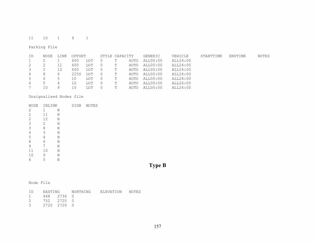
11 10 1 9 1 Parking File ID NODE LINK OFFSET STYLE CAPACITY GENERIC VEHICLE STARTTIME ENDTIME NOTES 1 2 1 600 LOT 0 T AUTO ALL00:00 ALL24:00 2 2 11 600 LOT 0 T AUTO ALL00:00 ALL24:00 3 2 12 600 LOT 0 T AUTO ALL00:00 ALL24:00 4 8 6 2250 LOT 0 T AUTO ALL00:00 ALL24:00 5 6 5 10 LOT 0 T AUTO ALL00:00 ALL24:00 6 5 4 10 LOT 0 T AUTO ALL00:00 ALL24:00 7 10 9 10 LOT 0 T AUTO ALL00:00 ALL24:00 Unsignalised Nodes file NODE INLINK SIGN NOTES 2 1 N 2 11 N 2 12 N 3 2 N 3 8 N 4 3 N 5 4 N 8 6 N 9 7 N 11 10 N 10 9 N 6 5 N

Type B Node File ID EASTING NORTHING ELEVATION NOTES 1 448 2736 0 2 752 2720 0 3 2720 2720 0

157

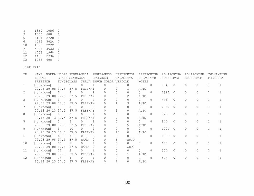
8 1360 1056 0 9 1056 608 0 5 3184 2720 0 6 4096 3024 0 10 4096 2272 0 7 5008 3632 0 11 4704 1968 0 12 448 2736 1 13 1056 608 1 Link File ID NAME NODEA NODEB PERMLANESA PERMLANESB LEFTPCKTSA LEFTPCKTSB RGHTPCKTSA RGHTPCKTSB TWOWAYTURN LENGTH GRADE SETBACKA SETBACKB CAPACITYA CAPACITYB SPEEDLMTA SPEEDLMTB FREESPDA FREESPDB FUNCTCLASS THRUA THRUB COLOR VEHICLE NOTES 1 [unknown] 1 2 0 1 0 0 0 0 0 304 0 0 0 1 1 29.08 29.08 37.5 37.5 FREEWAY 0 2 1 AUTO 2 [unknown] 2 3 0 2 0 0 0 0 0 1824 0 0 0 1 1 29.08 29.08 37.5 37.5 FREEWAY 0 3 2 AUTO 3 [unknown] 3 5 0 4 0 0 0 0 0 448 0 0 0 1 1 29.08 29.08 37.5 37.5 FREEWAY 0 4 3 AUTO 7 [unknown] 8 3 0 2 0 0 0 0 0 2064 0 0 0 1 1 20.13 20.13 37.5 37.5 FREEWAY 0 3 0 AUTO 8 [unknown] 9 8 0 1 0 0 0 0 0 528 0 0 0 1 1 20.13 20.13 37.5 37.5 FREEWAY 0 7 0 AUTO 5 [unknown] 5 6 0 3 0 0 0 0 0 944 0 0 0 1 1 29.08 29.08 37.5 37.5 FREEWAY 0 6 5 AUTO 9 [unknown] 5 10 0 2 0 0 0 0 0 1024 0 0 0 1 1 20.13 20.13 37.5 37.5 FREEWAY 0 10 0 AUTO 6 [unknown] 6 7 0 3 0 0 0 0 0 1088 0 0 0 1 1 29.08 29.08 37.5 37.5 RAMP 0 0 6 AUTO 10 [unknown] 10 11 0 2 0 0 0 0 0 688 0 0 0 1 1 29.08 29.08 37.5 37.5 RAMP 0 0 0 AUTO 11 [unknown] 12 2 0 1 0 0 0 0 0 304 0 0 0 1 1 29.08 29.08 37.5 37.5 FREEWAY 0 2 1 AUTO 12 [unknown] 13 8 0 1 0 0 0 0 0 528 0 0 0 1 1 20.13 20.13 37.5 37.5 FREEWAY 0 7 0 AUTO

158

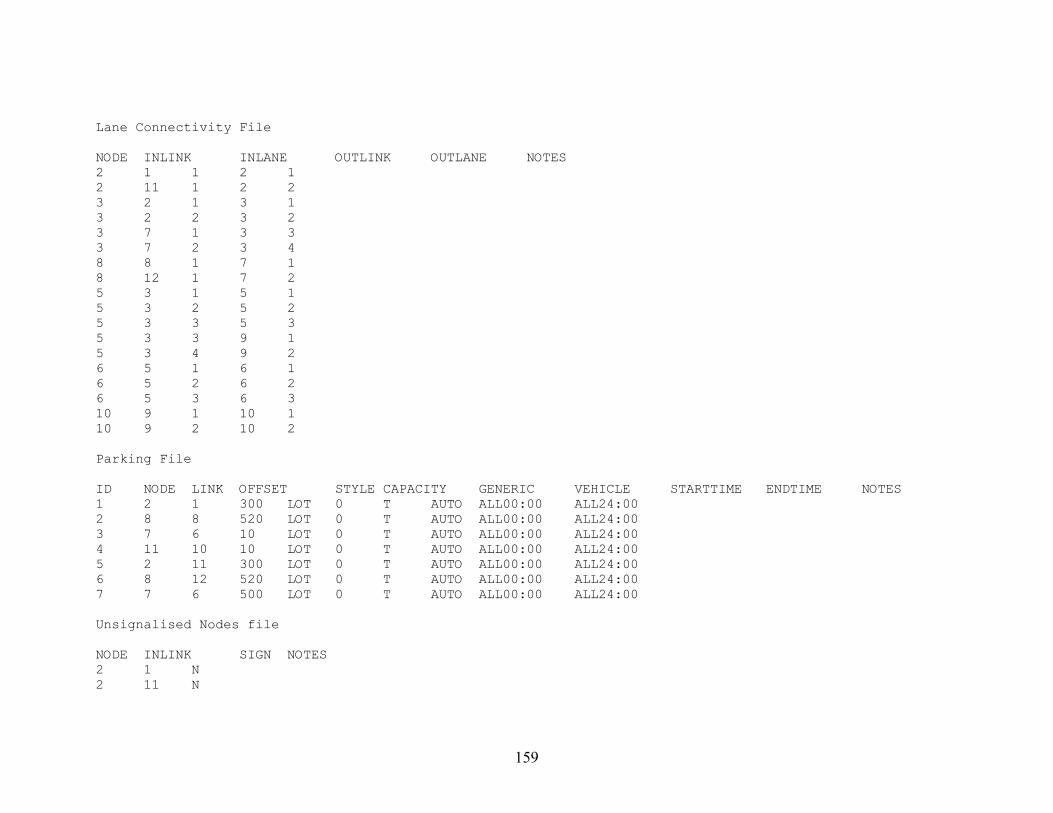
Lane Connectivity File NODE INLINK INLANE OUTLINK OUTLANE NOTES 2 1 1 2 1 2 11 1 2 2 3 2 1 3 1 3 2 2 3 2 3 7 1 3 3 3 7 2 3 4 8 8 1 7 1 8 12 1 7 2 5 3 1 5 1 5 3 2 5 2 5 3 3 5 3 5 3 3 9 1 5 3 4 9 2 6 5 1 6 1 6 5 2 6 2 6 5 3 6 3 10 9 1 10 1 10 9 2 10 2 Parking File ID NODE LINK OFFSET STYLE CAPACITY GENERIC VEHICLE STARTTIME ENDTIME NOTES 1 2 1 300 LOT 0 T AUTO ALL00:00 ALL24:00 2 8 8 520 LOT 0 T AUTO ALL00:00 ALL24:00 3 7 6 10 LOT 0 T AUTO ALL00:00 ALL24:00 4 11 10 10 LOT 0 T AUTO ALL00:00 ALL24:00 5 2 11 300 LOT 0 T AUTO ALL00:00 ALL24:00 6 8 12 520 LOT 0 T AUTO ALL00:00 ALL24:00 7 7 6 500 LOT 0 T AUTO ALL00:00 ALL24:00 Unsignalised Nodes file NODE INLINK SIGN NOTES 2 1 N 2 11 N

159

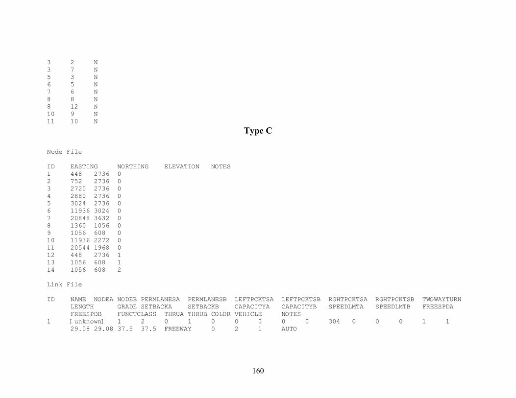
3 2 N 3 7 N 5 3 N 6 5 N 7 6 N 8 8 N 8 12 N 10 9 N 11 10 N

Type C Node File ID EASTING NORTHING ELEVATION NOTES 1 448 2736 0 2 752 2736 0 3 2720 2736 0 4 2880 2736 0 5 3024 2736 0 6 11936 3024 0 7 20848 3632 0 8 1360 1056 0 9 1056 608 0 10 11936 2272 0 11 20544 1968 0 12 448 2736 1 13 1056 608 1 14 1056 608 2 Link File ID NAME NODEA NODEB PERMLANESA PERMLANESB LEFTPCKTSA LEFTPCKTSB RGHTPCKTSA RGHTPCKTSB TWOWAYTURN LENGTH GRADE SETBACKA SETBACKB CAPACITYA CAPACITYB SPEEDLMTA SPEEDLMTB FREESPDA FREESPDB FUNCTCLASS THRUA THRUB COLOR VEHICLE NOTES 1 [unknown] 1 2 0 1 0 0 0 0 0 304 0 0 0 1 1 29.08 29.08 37.5 37.5 FREEWAY 0 2 1 AUTO

160

2 [unknown] 2 3 0 2 0 0 0 0 0 1824 0 0 0 1 1 29.08 29.08 37.5 37.5 FREEWAY 0 3 2 AUTO 3 [unknown] 3 4 0 5 0 0 0 0 0 144 0 0 0 1 1 29.08 29.08 37.5 37.5 FREEWAY 0 4 3 AUTO 4 [unknown] 4 5 0 5 0 0 0 0 0 144 0 0 0 1 1 29.08 29.08 37.5 37.5 FREEWAY 0 5 4 AUTO 5 [unknown] 5 6 0 3 0 0 0 0 0 8917 0 0 0 1 1 29.08 29.08 37.5 37.5 FREEWAY 0 6 5 AUTO 6 [unknown] 6 7 0 3 0 0 0 0 0 8933 0 0 0 1 1 29.08 29.08 37.5 37.5 RAMP 0 0 6 AUTO 7 [unknown] 8 3 0 3 0 0 0 0 0 2064 0 0 0 1 1 20.13 20.13 37.5 37.5 FREEWAY 0 3 0 AUTO 8 [unknown] 9 8 0 1 0 0 0 0 0 528 0 0 0 1 1 20.13 20.13 37.5 37.5 FREEWAY 0 7 0 AUTO 9 [unknown] 5 10 0 2 0 0 0 0 0 8924 0 0 0 1 1 20.13 20.13 37.5 37.5 FREEWAY 0 10 0 AUTO 10 [unknown] 10 11 0 2 0 0 0 0 0 8613 0 0 0 1 1 20.13 20.13 37.5 37.5 FREEWAY 0 0 0 AUTO 11 [unknown] 12 2 0 1 0 0 0 0 0 304 0 0 0 1 1 29.08 29.08 37.5 37.5 FREEWAY 0 2 1 AUTO 12 [unknown] 13 8 0 1 0 0 0 0 0 528 0 0 0 1 1 20.13 20.13 37.5 37.5 FREEWAY 0 7 0 AUTO 13 [unknown] 14 8 0 1 0 0 0 0 0 528 0 0 0 1 1 20.13 20.13 37.5 37.5 FREEWAY 0 7 0 AUTO Lane Connectivity File NODE INLINK INLANE OUTLINK OUTLANE NOTES 2 1 1 2 1 2 11 1 2 1 3 2 1 3 1 3 2 2 3 2 3 7 1 3 3 3 7 2 3 4 3 7 3 3 5 4 3 1 4 1 4 3 2 4 2 4 3 3 4 3

161

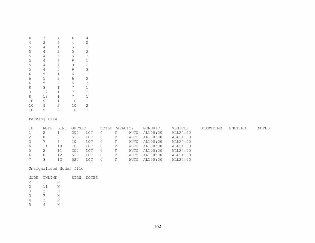
4 3 4 4 4 4 3 5 4 5 5 4 1 5 1 5 4 2 5 2 5 4 3 5 3 5 4 3 9 1 5 4 4 9 2 5 4 5 9 3 6 5 1 6 1 6 5 2 6 2 6 5 3 6 3 8 8 1 7 1 8 12 1 7 1 8 13 1 7 1 10 9 1 10 1 10 9 2 10 2 10 9 3 10 3 Parking File ID NODE LINK OFFSET STYLE CAPACITY GENERIC VEHICLE STARTTIME ENDTIME NOTES 1 2 1 300 LOT 0 T AUTO ALL00:00 ALL24:00 2 8 8 520 LOT 0 T AUTO ALL00:00 ALL24:00 3 7 6 10 LOT 0 T AUTO ALL00:00 ALL24:00 4 11 10 10 LOT 0 T AUTO ALL00:00 ALL24:00 5 2 11 300 LOT 0 T AUTO ALL00:00 ALL24:00 6 8 12 520 LOT 0 T AUTO ALL00:00 ALL24:00 7 8 13 520 LOT 0 T AUTO ALL00:00 ALL24:00 Unsignalised Nodes file NODE INLINK SIGN NOTES 2 1 N 2 11 N 3 2 N 3 7 N 4 3 N 5 4 N

162

6 5 N 7 6 N 8 8 N 8 12 N 8 13 N 10 9 N 11 10 N

163

APPENDIX C

164

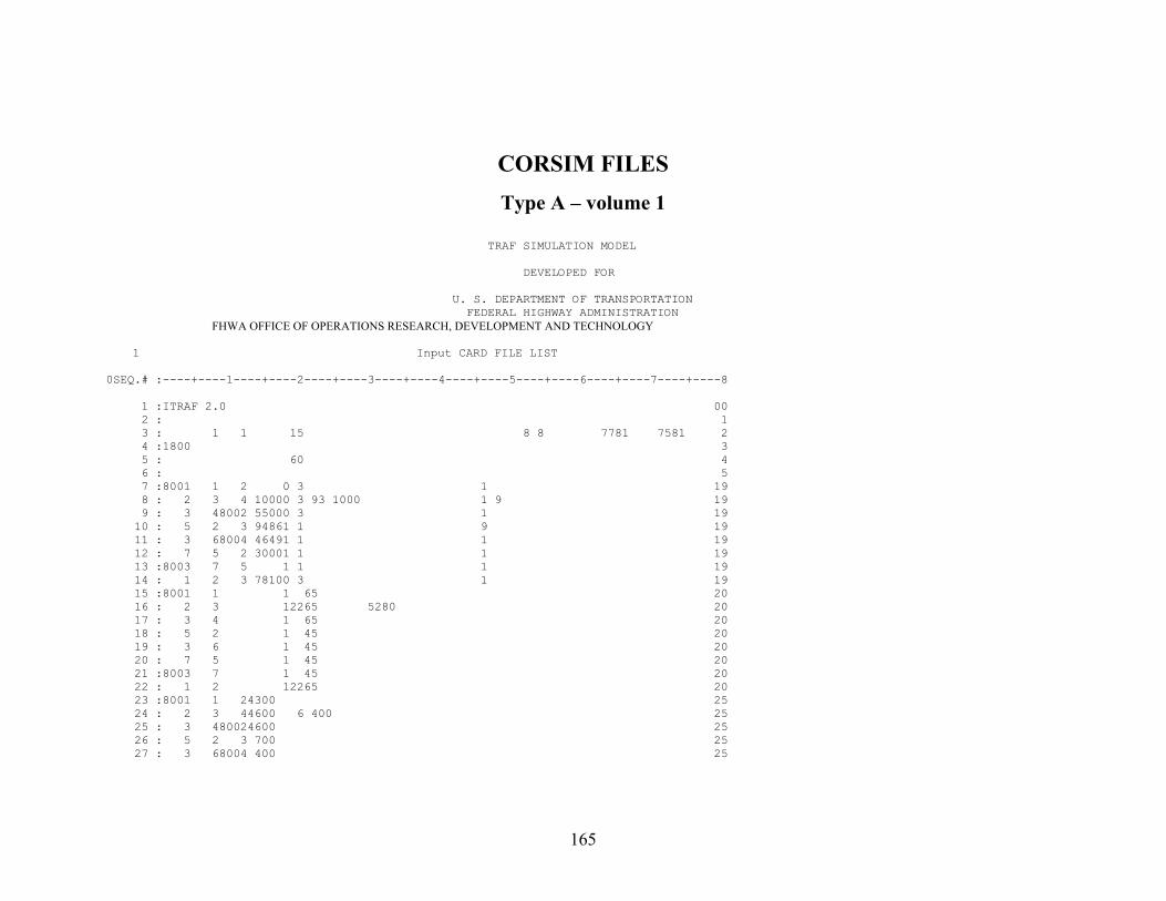
CORSIM FILES Type A – volume 1

TRAF SIMULATION MODEL DEVELOPED FOR U. S. DEPARTMENT OF TRANSPORTATION FEDERAL HIGHWAY ADMINISTRATION FHWA OFFICE OF OPERATIONS RESEARCH, DEVELOPMENT AND TECHNOLOGY

1 Input CARD FILE LIST

0SEQ.# :----+----1----+----2----+----3----+----4----+----5----+----6----+----7----+----8 1 :ITRAF 2.0 00 2 : 1 3 : 1 1 15 8 8 7781 7581 2 4 :1800 3 5 : 60 4 6 : 5 7 :8001 1 2 0 3 1 19 8 : 2 3 4 10000 3 93 1000 1 9 19 9 : 3 48002 55000 3 1 19 10 : 5 2 3 94861 1 9 19 11 : 3 68004 46491 1 1 19 12 : 7 5 2 30001 1 1 19 13 :8003 7 5 1 1 1 19 14 : 1 2 3 78100 3 1 19 15 :8001 1 1 65 20 16 : 2 3 12265 5280 20 17 : 3 4 1 65 20 18 : 5 2 1 45 20 19 : 3 6 1 45 20 20 : 7 5 1 45 20 21 :8003 7 1 45 20 22 : 1 2 12265 20 23 :8001 1 24300 25 24 : 2 3 44600 6 400 25 25 : 3 480024600 25 26 : 5 2 3 700 25 27 : 3 68004 400 25

165

28 : 7 5 2 700 25 29 :8003 7 5 700 25 30 : 1 2 34300 25 31 : 2 3 9 40 20 10 2 1 28 32 : 2 3 1 40 20 10 2 2 28 33 : 2 3 2 40 20 10 2 2 28 34 : 2 3 3 40 20 10 2 2 28 35 : 2 3 9 200 20 10 2 3 28 36 : 2 3 1 200 20 10 2 4 28 37 : 2 3 2 200 20 10 2 4 28 38 : 2 3 3 200 20 10 2 4 28 39 : 2 3 9 500 20 10 2 5 28 40 : 2 3 1 500 20 10 2 6 28 41 : 2 3 2 500 20 10 2 6 28 42 : 2 3 3 500 20 10 2 6 28 43 : 2 3 9 980 20 10 2 7 28 44 : 2 3 1 980 20 10 2 8 28 45 : 2 3 2 980 20 10 2 8 28 46 : 2 3 3 980 20 10 2 8 28 47 :8001 14300 20 40 40 50 48 :8003 7 700 50 49 : 1 900 60 17 1 64 50 : 1 2 3 4 5 6 7 8 67 0SEQ.# :----+----1----+----2----+----3----+----4----+----5----+----6----+----7----+----8 1 CARD FILE LIST (CONT.) 0SEQ.# :----+----1----+----2----+----3----+----4----+----5----+----6----+----7----+----8 51 : 15 14 13 12 11 10 9 8 7 6 68 52 : 16 16 16 16 3 1 69 53 : 20 16 1 20 70 54 : 1 14 7 150 25 1 71 55 : 2 3 14 2 4 86 1 3 7 1 4 93 74 56 : 0 170 57 : 1 0 16000 195 58 : 2 6000 11000 195 59 : 3 7000 11000 195 60 : 4 12500 11000 195 61 : 5 3000 2000 195 62 : 6 10500 7500 195 63 :8001 0 14000 195 64 :8002 15500 11000 195 65 :8003 1000 9500 195 66 :8004 11500 4500 195 67 : 7 0 2000 195 68 : 1 210 0SEQ.# :----+----1----+----2----+----3----+----4----+----5----+----6----+----7----+----8

166

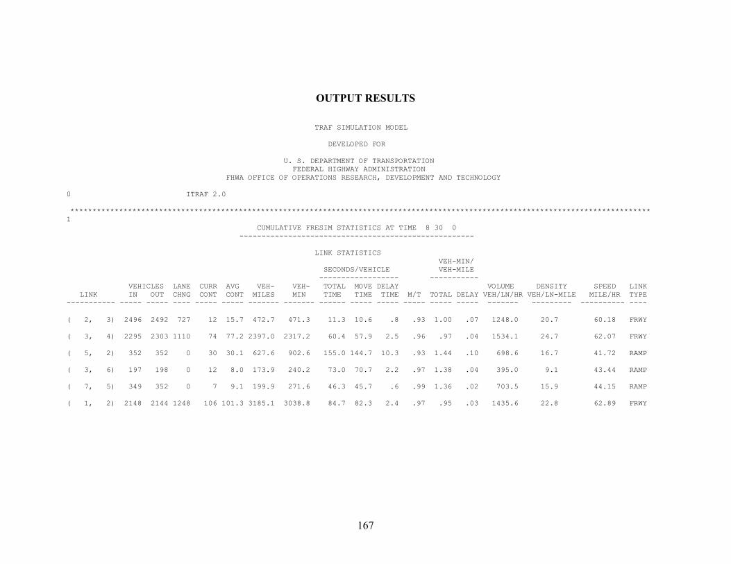
OUTPUT RESULTS

TRAF SIMULATION MODEL DEVELOPED FOR U. S. DEPARTMENT OF TRANSPORTATION FEDERAL HIGHWAY ADMINISTRATION FHWA OFFICE OF OPERATIONS RESEARCH, DEVELOPMENT AND TECHNOLOGY 0 ITRAF 2.0 *********************************************************************************************************************************** 1 CUMULATIVE FRESIM STATISTICS AT TIME 8 30 0 ----------------------------------------------------- LINK STATISTICS VEH-MIN/ SECONDS/VEHICLE VEH-MILE ------------------ ----------- VEHICLES LANE CURR AVG VEH- VEH- TOTAL MOVE DELAY VOLUME DENSITY SPEED LINK LINK IN OUT CHNG CONT CONT MILES MIN TIME TIME TIME M/T TOTAL DELAY VEH/LN/HR VEH/LN-MILE MILE/HR TYPE ----------- ----- ----- ---- ----- ----- ------- ------- ------ ----- ----- ----- ----- ----- ------- --------- ---------- ---- ( 2, 3) 2496 2492 727 12 15.7 472.7 471.3 11.3 10.6 .8 .93 1.00 .07 1248.0 20.7 60.18 FRWY ( 3, 4) 2295 2303 1110 74 77.2 2397.0 2317.2 60.4 57.9 2.5 .96 .97 .04 1534.1 24.7 62.07 FRWY ( 5, 2) 352 352 0 30 30.1 627.6 902.6 155.0 144.7 10.3 .93 1.44 .10 698.6 16.7 41.72 RAMP ( 3, 6) 197 198 0 12 8.0 173.9 240.2 73.0 70.7 2.2 .97 1.38 .04 395.0 9.1 43.44 RAMP ( 7, 5) 349 352 0 7 9.1 199.9 271.6 46.3 45.7 .6 .99 1.36 .02 703.5 15.9 44.15 RAMP ( 1, 2) 2148 2144 1248 106 101.3 3185.1 3038.8 84.7 82.3 2.4 .97 .95 .03 1435.6 22.8 62.89 FRWY

167

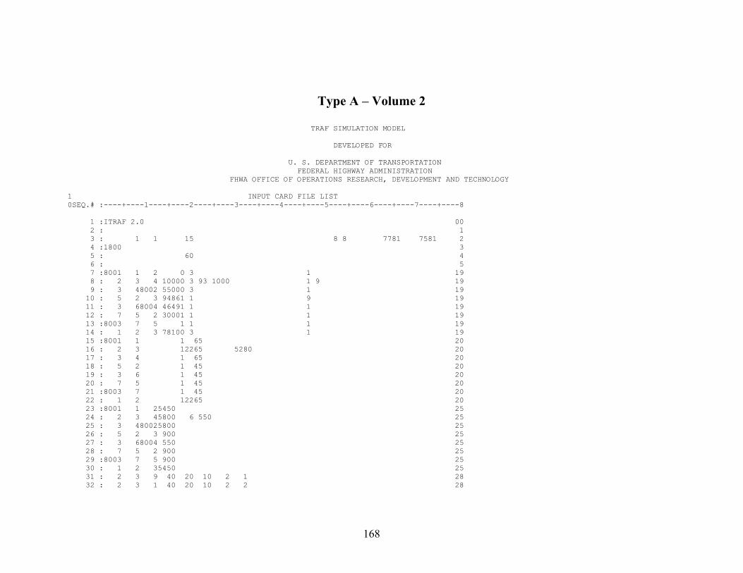
Type A – Volume 2

TRAF SIMULATION MODEL DEVELOPED FOR U. S. DEPARTMENT OF TRANSPORTATION FEDERAL HIGHWAY ADMINISTRATION FHWA OFFICE OF OPERATIONS RESEARCH, DEVELOPMENT AND TECHNOLOGY 1 INPUT CARD FILE LIST 0SEQ.# :----+----1----+----2----+----3----+----4----+----5----+----6----+----7----+----8 1 :ITRAF 2.0 00 2 : 1 3 : 1 1 15 8 8 7781 7581 2 4 :1800 3 5 : 60 4 6 : 5 7 :8001 1 2 0 3 1 19 8 : 2 3 4 10000 3 93 1000 1 9 19 9 : 3 48002 55000 3 1 19 10 : 5 2 3 94861 1 9 19 11 : 3 68004 46491 1 1 19 12 : 7 5 2 30001 1 1 19 13 :8003 7 5 1 1 1 19 14 : 1 2 3 78100 3 1 19 15 :8001 1 1 65 20 16 : 2 3 12265 5280 20 17 : 3 4 1 65 20 18 : 5 2 1 45 20 19 : 3 6 1 45 20 20 : 7 5 1 45 20 21 :8003 7 1 45 20 22 : 1 2 12265 20 23 :8001 1 25450 25 24 : 2 3 45800 6 550 25 25 : 3 480025800 25 26 : 5 2 3 900 25 27 : 3 68004 550 25 28 : 7 5 2 900 25 29 :8003 7 5 900 25 30 : 1 2 35450 25 31 : 2 3 9 40 20 10 2 1 28 32 : 2 3 1 40 20 10 2 2 28

168

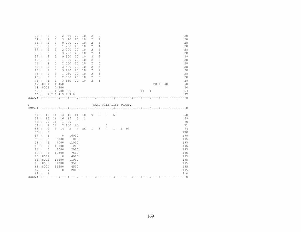
33 : 2 3 2 40 20 10 2 2 28 34 : 2 3 3 40 20 10 2 2 28 35 : 2 3 9 200 20 10 2 3 28 36 : 2 3 1 200 20 10 2 4 28 37 : 2 3 2 200 20 10 2 4 28 38 : 2 3 3 200 20 10 2 4 28 39 : 2 3 9 500 20 10 2 5 28 40 : 2 3 1 500 20 10 2 6 28 41 : 2 3 2 500 20 10 2 6 28 42 : 2 3 3 500 20 10 2 6 28 43 : 2 3 9 980 20 10 2 7 28 44 : 2 3 1 980 20 10 2 8 28 45 : 2 3 2 980 20 10 2 8 28 46 : 2 3 3 980 20 10 2 8 28 47 :8001 15450 20 40 40 50 48 :8003 7 900 50 49 : 1 900 60 17 1 64 50 : 1 2 3 4 5 6 7 8 67 0SEQ.# :----+----1----+----2----+----3----+----4----+----5----+----6----+----7----+----8 1 CARD FILE LIST (CONT.) 0SEQ.# :----+----1----+----2----+----3----+----4----+----5----+----6----+----7----+----8 51 : 15 14 13 12 11 10 9 8 7 6 68 52 : 16 16 16 16 3 1 69 53 : 20 16 1 20 70 54 : 1 14 7 150 25 1 71 55 : 2 3 14 2 4 86 1 3 7 1 4 93 74 56 : 0 170 57 : 1 0 16000 195 58 : 2 6000 11000 195 59 : 3 7000 11000 195 60 : 4 12500 11000 195 61 : 5 3000 2000 195 62 : 6 10500 7500 195 63 :8001 0 14000 195 64 :8002 15500 11000 195 65 :8003 1000 9500 195 66 :8004 11500 4500 195 67 : 7 0 2000 195 68 : 1 210 0SEQ.# :----+----1----+----2----+----3----+----4----+----5----+----6----+----7----+----8

169

OUTPUT RESULTS

TRAF SIMULATION MODEL DEVELOPED FOR U. S. DEPARTMENT OF TRANSPORTATION FEDERAL HIGHWAY ADMINISTRATION FHWA OFFICE OF OPERATIONS RESEARCH, DEVELOPMENT AND TECHNOLOGY 0 ITRAF 2.0 0 *********************************************************************************************************************************** 1 FRESIM LINK CHARACTERISTICS CUMULATIVE FRESIM STATISTICS AT TIME 8 30 0 ----------------------------------------------------- LINK STATISTICS VEH-MIN/ SECONDS/VEHICLE VEH-MILE ------------------ ----------- VEHICLES LANE CURR AVG VEH- VEH- TOTAL MOVE DELAY VOLUME DENSITY SPEED LINK LINK IN OUT CHNG CONT CONT MILES MIN TIME TIME TIME M/T TOTAL DELAY VEH/LN/HR VEH/LN-MILE MILE/HR TYPE ----------- ----- ----- ---- ----- ----- ------- ------- ------ ----- ----- ----- ----- ----- ------- --------- ---------- ---- ( 2, 3) 3180 3171 992 21 20.2 600.9 605.1 11.4 10.6 .9 .92 1.01 .08 1586.3 26.6 59.58 FRWY ( 3, 4) 2895 2895 1337 101 98.4 3021.1 2952.2 61.1 57.9 3.1 .95 .98 .05 1933.5 31.5 61.40 FRWY ( 5, 2) 450 454 0 38 38.8 808.8 1164.3 155.2 143.7 11.5 .93 1.44 .11 900.4 21.6 41.68 RAMP ( 3, 6) 276 280 0 10 11.3 243.0 339.9 73.9 70.9 3.0 .96 1.40 .06 552.0 12.9 42.90 RAMP ( 7, 5) 450 450 0 11 11.6 257.2 348.0 46.1 45.4 .7 .98 1.35 .02 905.4 20.4 44.35 RAMP ( 1, 2) 2724 2726 1544 129 129.8 4038.4 3892.9 85.6 82.4 3.2 .96 .96 .04 1820.1 29.2 62.24 FRWY

170

Type A – Volume 3 TRAF SIMULATION MODEL DEVELOPED FOR U. S. DEPARTMENT OF TRANSPORTATION FEDERAL HIGHWAY ADMINISTRATION FHWA OFFICE OF OPERATIONS RESEARCH, DEVELOPMENT AND TECHNOLOGY 1 INPUT CARD FILE LIST 0SEQ.# :----+----1----+----2----+----3----+----4----+----5----+----6----+----7----+----8 1 :ITRAF 2.0 00 2 : 1 3 : 1 1 15 8 8 7781 7581 2 4 :1800 3 5 : 60 4 6 : 5 7 :8001 1 2 0 3 1 19 8 : 2 3 4 10000 3 93 1000 1 9 19 9 : 3 48002 55000 3 1 19 10 : 5 2 3 94861 1 9 19 11 : 3 68004 46491 1 1 19 12 : 7 5 2 30001 1 1 19 13 :8003 7 5 1 1 1 19 14 : 1 2 3 78100 3 1 19 15 :8001 1 1 65 20 16 : 2 3 12265 5280 20 17 : 3 4 1 65 20 18 : 5 2 1 45 20 19 : 3 6 1 45 20 20 : 7 5 1 45 20 21 :8003 7 1 45 20 22 : 1 2 12265 20 23 :8001 1 26600 25 24 : 2 3 47000 6 700 25 25 : 3 480027000 25 26 : 5 2 31100 25 27 : 3 68004 700 25 28 : 7 5 21100 25 29 :8003 7 51100 25 30 : 1 2 36600 25 31 : 2 3 9 40 20 10 2 1 28 32 : 2 3 1 40 20 10 2 2 28

171

33 : 2 3 2 40 20 10 2 2 28 34 : 2 3 3 40 20 10 2 2 28 35 : 2 3 9 200 20 10 2 3 28 36 : 2 3 1 200 20 10 2 4 28 37 : 2 3 2 200 20 10 2 4 28 38 : 2 3 3 200 20 10 2 4 28 39 : 2 3 9 500 20 10 2 5 28 40 : 2 3 1 500 20 10 2 6 28 41 : 2 3 2 500 20 10 2 6 28 42 : 2 3 3 500 20 10 2 6 28 43 : 2 3 9 980 20 10 2 7 28 44 : 2 3 1 980 20 10 2 8 28 45 : 2 3 2 980 20 10 2 8 28 46 : 2 3 3 980 20 10 2 8 28 47 :8001 16600 20 40 40 50 48 :8003 71100 50 49 : 1 900 60 17 1 64 50 : 1 2 3 4 5 6 7 8 67 0SEQ.# :----+----1----+----2----+----3----+----4----+----5----+----6----+----7----+----8 1 CARD FILE LIST (CONT.) 0SEQ.# :----+----1----+----2----+----3----+----4----+----5----+----6----+----7----+----8 51 : 15 14 13 12 11 10 9 8 7 6 68 52 : 16 16 16 16 3 1 69 53 : 20 16 1 20 70 54 : 1 14 7 150 25 1 71 55 : 2 3 14 2 4 86 1 3 7 1 4 93 74 56 : 0 170 57 : 1 0 16000 195 58 : 2 6000 11000 195 59 : 3 7000 11000 195 60 : 4 12500 11000 195 61 : 5 3000 2000 195 62 : 6 10500 7500 195 63 :8001 0 14000 195 64 :8002 15500 11000 195 65 :8003 1000 9500 195 66 :8004 11500 4500 195 67 : 7 0 2000 195 68 : 1 210 0SEQ.# :----+----1----+----2----+----3----+----4----+----5----+----6----+----7----+----8

172

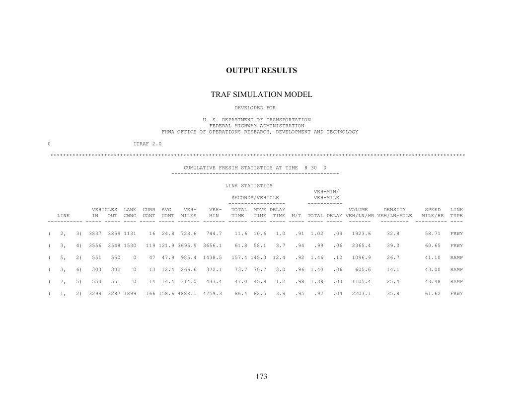
OUTPUT RESULTS

TRAF SIMULATION MODEL

DEVELOPED FOR U. S. DEPARTMENT OF TRANSPORTATION FEDERAL HIGHWAY ADMINISTRATION FHWA OFFICE OF OPERATIONS RESEARCH, DEVELOPMENT AND TECHNOLOGY 0 ITRAF 2.0 *********************************************************************************************************************************** CUMULATIVE FRESIM STATISTICS AT TIME 8 30 0 ----------------------------------------------------- LINK STATISTICS VEH-MIN/ SECONDS/VEHICLE VEH-MILE ------------------ ----------- VEHICLES LANE CURR AVG VEH- VEH- TOTAL MOVE DELAY VOLUME DENSITY SPEED LINK LINK IN OUT CHNG CONT CONT MILES MIN TIME TIME TIME M/T TOTAL DELAY VEH/LN/HR VEH/LN-MILE MILE/HR TYPE ----------- ----- ----- ---- ----- ----- ------- ------- ------ ----- ----- ----- ----- ----- ------- --------- ---------- ---- ( 2, 3) 3837 3859 1131 16 24.8 728.6 744.7 11.6 10.6 1.0 .91 1.02 .09 1923.6 32.8 58.71 FRWY ( 3, 4) 3556 3548 1530 119 121.9 3695.9 3656.1 61.8 58.1 3.7 .94 .99 .06 2365.4 39.0 60.65 FRWY ( 5, 2) 551 550 0 47 47.9 985.4 1438.5 157.4 145.0 12.4 .92 1.46 .12 1096.9 26.7 41.10 RAMP ( 3, 6) 303 302 0 13 12.4 266.6 372.1 73.7 70.7 3.0 .96 1.40 .06 605.6 14.1 43.00 RAMP ( 7, 5) 550 551 0 14 14.4 314.0 433.4 47.0 45.9 1.2 .98 1.38 .03 1105.4 25.4 43.48 RAMP ( 1, 2) 3299 3287 1899 166 158.6 4888.1 4759.3 86.4 82.5 3.9 .95 .97 .04 2203.1 35.8 61.62 FRWY

173

Type A – Volume 4

TRAF SIMULATION MODEL DEVELOPED FOR U. S. DEPARTMENT OF TRANSPORTATION FEDERAL HIGHWAY ADMINISTRATION FHWA OFFICE OF OPERATIONS RESEARCH, DEVELOPMENT AND TECHNOLOGY 1 CARD FILE LIST 0SEQ.# :----+----1----+----2----+----3----+----4----+----5----+----6----+----7----+----8 1 :ITRAF 2.0 00 2 : 1 3 : 1 1 15 8 8 7781 7581 2 4 :1800 3 5 : 60 4 6 : 5 7 :8001 1 2 0 3 1 19 8 : 2 3 4 10000 3 93 1000 1 9 19 9 : 3 48002 55000 3 1 19 10 : 5 2 3 94861 1 9 19 11 : 3 68004 46491 1 1 19 12 : 7 5 2 30001 1 1 19 13 :8003 7 5 1 1 1 19 14 : 1 2 3 78100 3 1 19 15 :8001 1 1 65 20 16 : 2 3 12265 5280 20 17 : 3 4 1 65 20 18 : 5 2 1 45 20 19 : 3 6 1 45 20 20 : 7 5 1 45 20 21 :8003 7 1 45 20 22 : 1 2 12265 20 23 :8001 1 26800 25 24 : 2 3 47200 61100 25 25 : 3 480027200 25 26 : 5 2 31500 25 27 : 3 680041100 25 28 : 7 5 21500 25 29 :8003 7 51500 25 30 : 1 2 36800 25 31 : 2 3 9 40 20 10 2 1 28

174

32 : 2 3 1 40 20 10 2 2 28 33 : 2 3 2 40 20 10 2 2 28 34 : 2 3 3 40 20 10 2 2 28 35 : 2 3 9 200 20 10 2 3 28 36 : 2 3 1 200 20 10 2 4 28 37 : 2 3 2 200 20 10 2 4 28 38 : 2 3 3 200 20 10 2 4 28 39 : 2 3 9 500 20 10 2 5 28 40 : 2 3 1 500 20 10 2 6 28 41 : 2 3 2 500 20 10 2 6 28 42 : 2 3 3 500 20 10 2 6 28 43 : 2 3 9 980 20 10 2 7 28 44 : 2 3 1 980 20 10 2 8 28 45 : 2 3 2 980 20 10 2 8 28 46 : 2 3 3 980 20 10 2 8 28 47 :8001 16800 20 40 40 50 48 :8003 71500 50 49 : 1 900 60 17 1 64 50 : 1 2 3 4 5 6 7 8 67 0SEQ.# :----+----1----+----2----+----3----+----4----+----5----+----6----+----7----+----8 1 CARD FILE LIST (CONT.) 0SEQ.# :----+----1----+----2----+----3----+----4----+----5----+----6----+----7----+----8 51 : 15 14 13 12 11 10 9 8 7 6 68 52 : 16 16 16 16 3 1 69 53 : 20 16 1 20 70 54 : 1 14 7 150 25 1 71 55 : 2 3 14 2 4 86 1 3 7 1 4 93 74 56 : 0 170 57 : 1 0 16000 195 58 : 2 6000 11000 195 59 : 3 7000 11000 195 60 : 4 12500 11000 195 61 : 5 3000 2000 195 62 : 6 10500 7500 195 63 :8001 0 14000 195 64 :8002 15500 11000 195 65 :8003 1000 9500 195 66 :8004 11500 4500 195 67 : 7 0 2000 195 68 : 1 210 0SEQ.# :----+----1----+----2----+----3----+----4----+----5----+----6----+----7----+----8

175

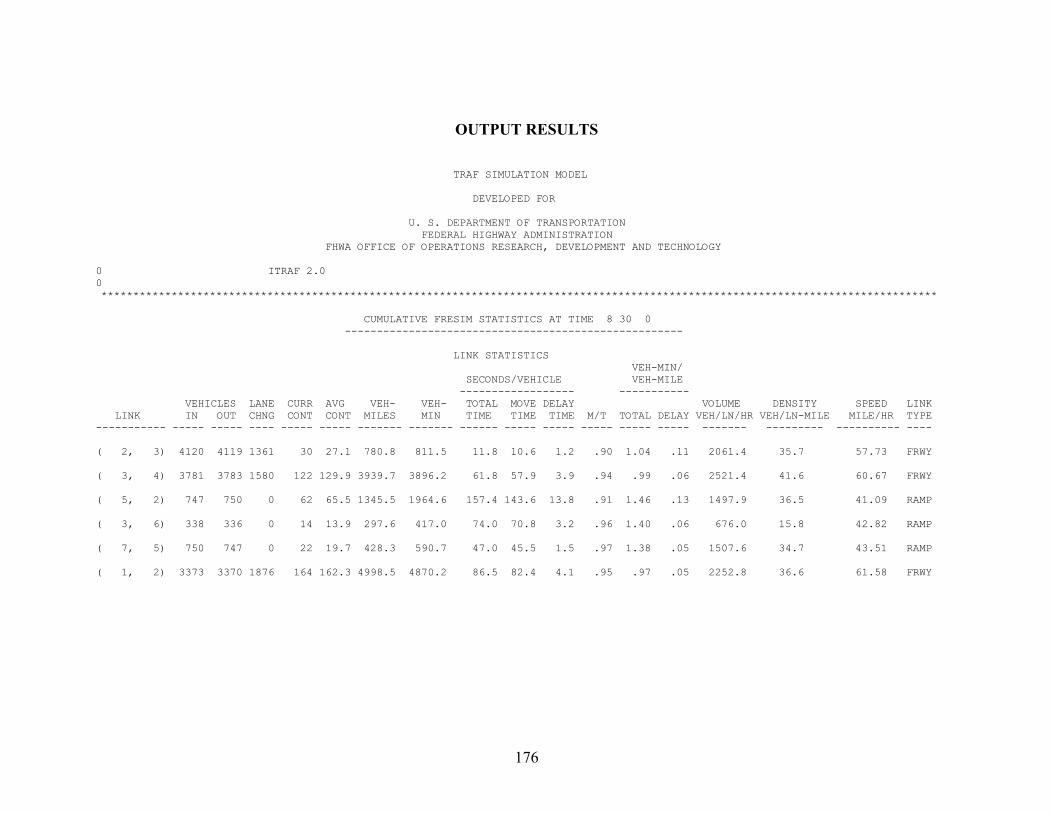
OUTPUT RESULTS

TRAF SIMULATION MODEL DEVELOPED FOR U. S. DEPARTMENT OF TRANSPORTATION FEDERAL HIGHWAY ADMINISTRATION FHWA OFFICE OF OPERATIONS RESEARCH, DEVELOPMENT AND TECHNOLOGY 0 ITRAF 2.0 0 *********************************************************************************************************************************** CUMULATIVE FRESIM STATISTICS AT TIME 8 30 0 ----------------------------------------------------- LINK STATISTICS VEH-MIN/ SECONDS/VEHICLE VEH-MILE ------------------ ----------- VEHICLES LANE CURR AVG VEH- VEH- TOTAL MOVE DELAY VOLUME DENSITY SPEED LINK LINK IN OUT CHNG CONT CONT MILES MIN TIME TIME TIME M/T TOTAL DELAY VEH/LN/HR VEH/LN-MILE MILE/HR TYPE ----------- ----- ----- ---- ----- ----- ------- ------- ------ ----- ----- ----- ----- ----- ------- --------- ---------- ---- ( 2, 3) 4120 4119 1361 30 27.1 780.8 811.5 11.8 10.6 1.2 .90 1.04 .11 2061.4 35.7 57.73 FRWY ( 3, 4) 3781 3783 1580 122 129.9 3939.7 3896.2 61.8 57.9 3.9 .94 .99 .06 2521.4 41.6 60.67 FRWY ( 5, 2) 747 750 0 62 65.5 1345.5 1964.6 157.4 143.6 13.8 .91 1.46 .13 1497.9 36.5 41.09 RAMP ( 3, 6) 338 336 0 14 13.9 297.6 417.0 74.0 70.8 3.2 .96 1.40 .06 676.0 15.8 42.82 RAMP ( 7, 5) 750 747 0 22 19.7 428.3 590.7 47.0 45.5 1.5 .97 1.38 .05 1507.6 34.7 43.51 RAMP ( 1, 2) 3373 3370 1876 164 162.3 4998.5 4870.2 86.5 82.4 4.1 .95 .97 .05 2252.8 36.6 61.58 FRWY

176

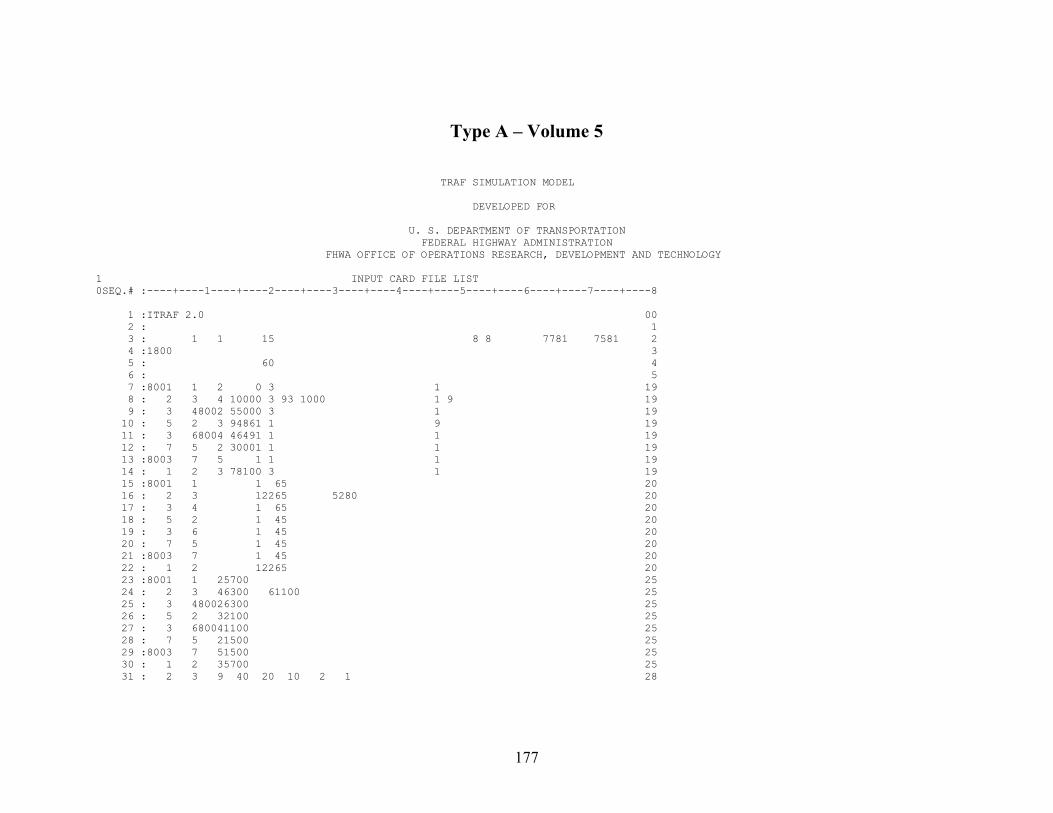
Type A – Volume 5 TRAF SIMULATION MODEL DEVELOPED FOR U. S. DEPARTMENT OF TRANSPORTATION FEDERAL HIGHWAY ADMINISTRATION FHWA OFFICE OF OPERATIONS RESEARCH, DEVELOPMENT AND TECHNOLOGY 1 INPUT CARD FILE LIST 0SEQ.# :----+----1----+----2----+----3----+----4----+----5----+----6----+----7----+----8 1 :ITRAF 2.0 00 2 : 1 3 : 1 1 15 8 8 7781 7581 2 4 :1800 3 5 : 60 4 6 : 5 7 :8001 1 2 0 3 1 19 8 : 2 3 4 10000 3 93 1000 1 9 19 9 : 3 48002 55000 3 1 19 10 : 5 2 3 94861 1 9 19 11 : 3 68004 46491 1 1 19 12 : 7 5 2 30001 1 1 19 13 :8003 7 5 1 1 1 19 14 : 1 2 3 78100 3 1 19 15 :8001 1 1 65 20 16 : 2 3 12265 5280 20 17 : 3 4 1 65 20 18 : 5 2 1 45 20 19 : 3 6 1 45 20 20 : 7 5 1 45 20 21 :8003 7 1 45 20 22 : 1 2 12265 20 23 :8001 1 25700 25 24 : 2 3 46300 61100 25 25 : 3 480026300 25 26 : 5 2 32100 25 27 : 3 680041100 25 28 : 7 5 21500 25 29 :8003 7 51500 25 30 : 1 2 35700 25 31 : 2 3 9 40 20 10 2 1 28

177

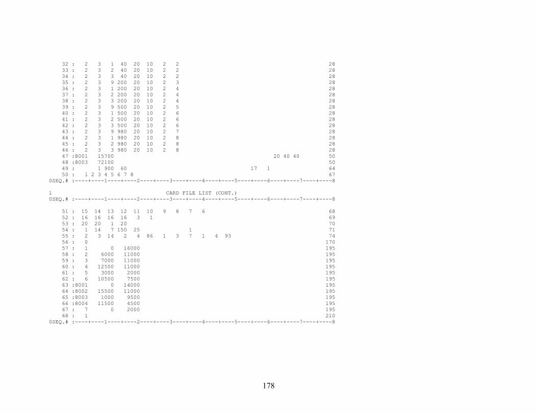
32 : 2 3 1 40 20 10 2 2 28 33 : 2 3 2 40 20 10 2 2 28 34 : 2 3 3 40 20 10 2 2 28 35 : 2 3 9 200 20 10 2 3 28 36 : 2 3 1 200 20 10 2 4 28 37 : 2 3 2 200 20 10 2 4 28 38 : 2 3 3 200 20 10 2 4 28 39 : 2 3 9 500 20 10 2 5 28 40 : 2 3 1 500 20 10 2 6 28 41 : 2 3 2 500 20 10 2 6 28 42 : 2 3 3 500 20 10 2 6 28 43 : 2 3 9 980 20 10 2 7 28 44 : 2 3 1 980 20 10 2 8 28 45 : 2 3 2 980 20 10 2 8 28 46 : 2 3 3 980 20 10 2 8 28 47 :8001 15700 20 40 40 50 48 :8003 72100 50 49 : 1 900 60 17 1 64 50 : 1 2 3 4 5 6 7 8 67 0SEQ.# :----+----1----+----2----+----3----+----4----+----5----+----6----+----7----+----8 1 CARD FILE LIST (CONT.) 0SEQ.# :----+----1----+----2----+----3----+----4----+----5----+----6----+----7----+----8 51 : 15 14 13 12 11 10 9 8 7 6 68 52 : 16 16 16 16 3 1 69 53 : 20 20 1 20 70 54 : 1 14 7 150 25 1 71 55 : 2 3 14 2 4 86 1 3 7 1 4 93 74 56 : 0 170 57 : 1 0 16000 195 58 : 2 6000 11000 195 59 : 3 7000 11000 195 60 : 4 12500 11000 195 61 : 5 3000 2000 195 62 : 6 10500 7500 195 63 :8001 0 14000 195 64 :8002 15500 11000 195 65 :8003 1000 9500 195 66 :8004 11500 4500 195 67 : 7 0 2000 195 68 : 1 210 0SEQ.# :----+----1----+----2----+----3----+----4----+----5----+----6----+----7----+----8

178

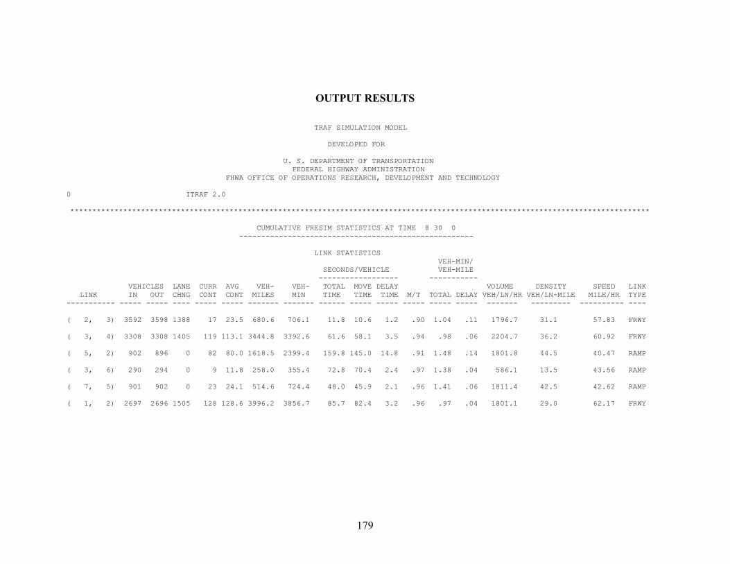
OUTPUT RESULTS

TRAF SIMULATION MODEL DEVELOPED FOR U. S. DEPARTMENT OF TRANSPORTATION FEDERAL HIGHWAY ADMINISTRATION FHWA OFFICE OF OPERATIONS RESEARCH, DEVELOPMENT AND TECHNOLOGY 0 ITRAF 2.0 *********************************************************************************************************************************** CUMULATIVE FRESIM STATISTICS AT TIME 8 30 0 ----------------------------------------------------- LINK STATISTICS VEH-MIN/ SECONDS/VEHICLE VEH-MILE ------------------ ----------- VEHICLES LANE CURR AVG VEH- VEH- TOTAL MOVE DELAY VOLUME DENSITY SPEED LINK LINK IN OUT CHNG CONT CONT MILES MIN TIME TIME TIME M/T TOTAL DELAY VEH/LN/HR VEH/LN-MILE MILE/HR TYPE ----------- ----- ----- ---- ----- ----- ------- ------- ------ ----- ----- ----- ----- ----- ------- --------- ---------- ---- ( 2, 3) 3592 3598 1388 17 23.5 680.6 706.1 11.8 10.6 1.2 .90 1.04 .11 1796.7 31.1 57.83 FRWY ( 3, 4) 3308 3308 1405 119 113.1 3444.8 3392.6 61.6 58.1 3.5 .94 .98 .06 2204.7 36.2 60.92 FRWY ( 5, 2) 902 896 0 82 80.0 1618.5 2399.4 159.8 145.0 14.8 .91 1.48 .14 1801.8 44.5 40.47 RAMP ( 3, 6) 290 294 0 9 11.8 258.0 355.4 72.8 70.4 2.4 .97 1.38 .04 586.1 13.5 43.56 RAMP ( 7, 5) 901 902 0 23 24.1 514.6 724.4 48.0 45.9 2.1 .96 1.41 .06 1811.4 42.5 42.62 RAMP ( 1, 2) 2697 2696 1505 128 128.6 3996.2 3856.7 85.7 82.4 3.2 .96 .97 .04 1801.1 29.0 62.17 FRWY

179

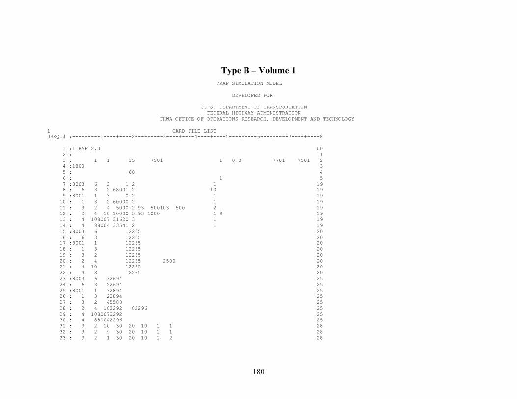
Type B – Volume 1 TRAF SIMULATION MODEL DEVELOPED FOR U. S. DEPARTMENT OF TRANSPORTATION FEDERAL HIGHWAY ADMINISTRATION FHWA OFFICE OF OPERATIONS RESEARCH, DEVELOPMENT AND TECHNOLOGY 1 CARD FILE LIST 0SEQ.# :----+----1----+----2----+----3----+----4----+----5----+----6----+----7----+----8 1 :ITRAF 2.0 00 2 : 1 3 : 1 1 15 7981 1 8 8 7781 7581 2 4 :1800 3 5 : 60 4 6 : 1 5 7 :8003 6 3 1 2 1 19 8 : 6 3 2 68001 2 10 19 9 :8001 1 3 0 2 1 19 10 : 1 3 2 60000 2 1 19 11 : 3 2 4 5000 2 93 500103 500 2 19 12 : 2 4 10 10000 3 93 1000 1 9 19 13 : 4 108007 31620 3 1 19 14 : 4 88004 33541 2 1 19 15 :8003 6 12265 20 16 : 6 3 12265 20 17 :8001 1 12265 20 18 : 1 3 12265 20 19 : 3 2 12265 20 20 : 2 4 12265 2500 20 21 : 4 10 12265 20 22 : 4 8 12265 20 23 :8003 6 32694 25 24 : 6 3 22694 25 25 :8001 1 32894 25 26 : 1 3 22894 25 27 : 3 2 45588 25 28 : 2 4 103292 82296 25 29 : 4 1080073292 25 30 : 4 880042296 25 31 : 3 2 10 30 20 10 2 1 28 32 : 3 2 9 30 20 10 2 1 28 33 : 3 2 1 30 20 10 2 2 28

180

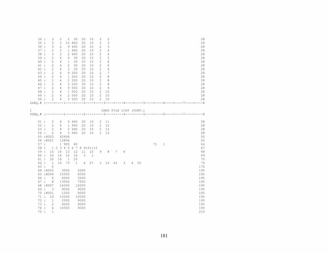
34 : 3 2 2 30 20 10 2 2 28 35 : 3 2 10 460 20 10 2 3 28 36 : 3 2 9 460 20 10 2 3 28 37 : 3 2 1 460 20 10 2 4 28 38 : 3 2 2 460 20 10 2 4 28 39 : 2 4 9 30 20 10 2 5 28 40 : 2 4 1 30 20 10 2 6 28 41 : 2 4 2 30 20 10 2 6 28 42 : 2 4 3 30 20 10 2 6 28 43 : 2 4 9 200 20 10 2 7 28 44 : 2 4 1 200 20 10 2 8 28 45 : 2 4 2 200 20 10 2 8 28 46 : 2 4 3 200 20 10 2 8 28 47 : 2 4 9 500 20 10 2 9 28 48 : 2 4 1 500 20 10 2 10 28 49 : 2 4 2 500 20 10 2 10 28 50 : 2 4 3 500 20 10 2 10 28 0SEQ.# :----+----1----+----2----+----3----+----4----+----5----+----6----+----7----+----8 1 CARD FILE LIST (CONT.) 0SEQ.# :----+----1----+----2----+----3----+----4----+----5----+----6----+----7----+----8 51 : 2 4 9 940 20 10 2 11 28 52 : 2 4 1 940 20 10 2 12 28 53 : 2 4 2 940 20 10 2 12 28 54 : 2 4 3 940 20 10 2 12 28 55 :8003 62694 50 56 :8001 12894 50 57 : 1 900 60 71 1 64 58 : 1 2 3 4 5 6 7 8 9101112 67 59 : 15 14 13 12 11 10 9 8 7 6 68 60 : 16 16 16 16 3 1 69 61 : 20 16 1 20 70 62 : 1 10 73 1 4 27 3 10 45 3 4 55 74 63 : 0 170 64 :8003 3500 2000 195 65 :8004 15500 6500 195 66 : 6 4500 3500 195 67 : 8 13500 7500 195 68 :8007 16500 12000 195 69 : 3 9000 9000 195 70 :8001 1500 9000 195 71 : 10 13500 10000 195 72 : 1 2500 9000 195 73 : 2 9500 9000 195 74 : 4 10500 9000 195 75 : 1 210

181

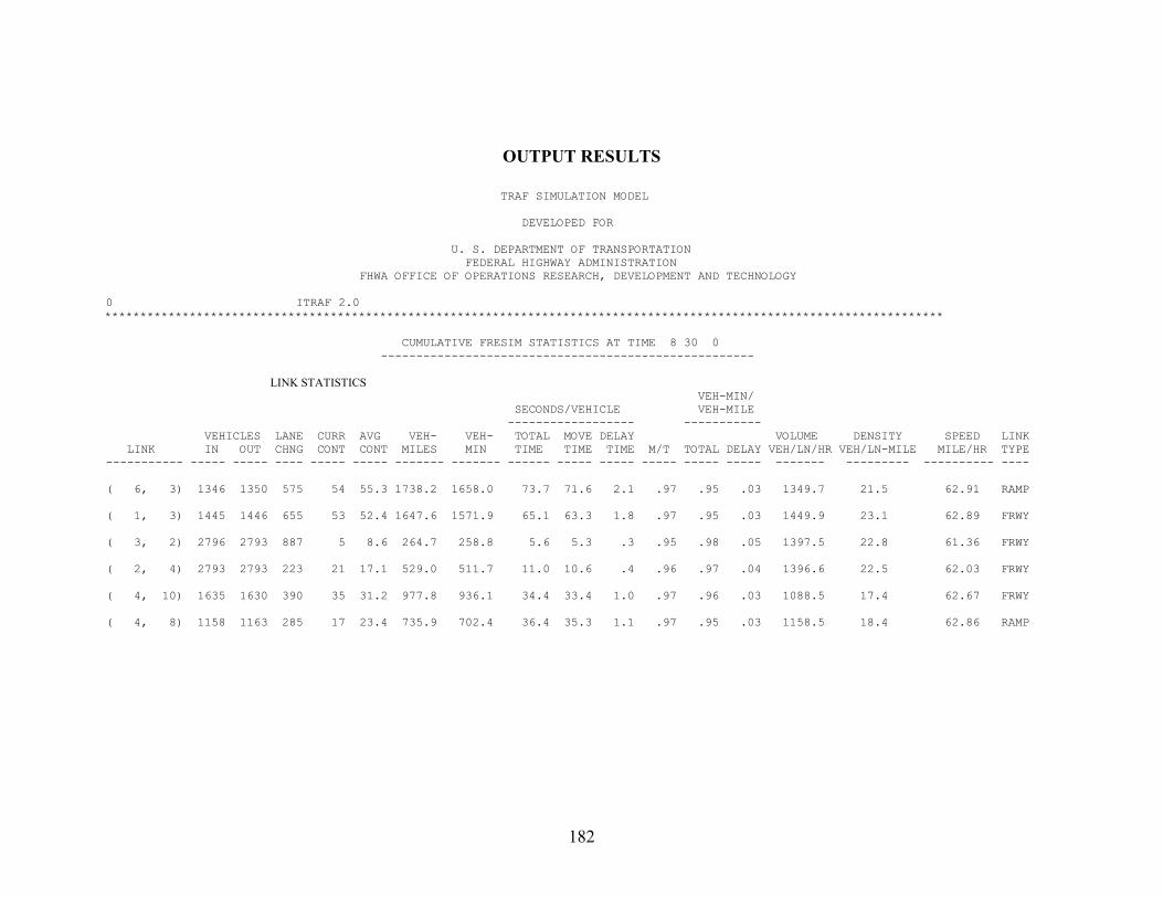
LINK STATISTICS

( 1, 3) 1445 1446 655 53 52.4 1647.6 1571.9 65.1 63.3 1.8 .97 .95 .03 1449.9 23.1 62.89 FRWY

( 3, 2) 2796 2793 887 5 8.6 264.7 258.8 5.6 5.3 .3 .95 .98 .05 1397.5 22.8 61.36 FRWY

OUTPUT RESULTS

TRAF SIMULATION MODEL DEVELOPED FOR U. S. DEPARTMENT OF TRANSPORTATION FEDERAL HIGHWAY ADMINISTRATION FHWA OFFICE OF OPERATIONS RESEARCH, DEVELOPMENT AND TECHNOLOGY 0 ITRAF 2.0 *********************************************************************************************************************** CUMULATIVE FRESIM STATISTICS AT TIME 8 30 0 ----------------------------------------------------- VEH-MIN/ SECONDS/VEHICLE VEH-MILE ------------------ ----------- VEHICLES LANE CURR AVG VEH- VEH- TOTAL MOVE DELAY VOLUME DENSITY SPEED LINK LINK IN OUT CHNG CONT CONT MILES MIN TIME TIME TIME M/T TOTAL DELAY VEH/LN/HR VEH/LN-MILE MILE/HR TYPE ----------- ----- ----- ---- ----- ----- ------- ------- ------ ----- ----- ----- ----- ----- ------- --------- ---------- ---- ( 6, 3) 1346 1350 575 54 55.3 1738.2 1658.0 73.7 71.6 2.1 .97 .95 .03 1349.7 21.5 62.91 RAMP

( 2, 4) 2793 2793 223 21 17.1 529.0 511.7 11.0 10.6 .4 .96 .97 .04 1396.6 22.5 62.03 FRWY ( 4, 10) 1635 1630 390 35 31.2 977.8 936.1 34.4 33.4 1.0 .97 .96 .03 1088.5 17.4 62.67 FRWY ( 4, 8) 1158 1163 285 17 23.4 735.9 702.4 36.4 35.3 1.1 .97 .95 .03 1158.5 18.4 62.86 RAMP

182

Type B – Volume 2 TRAF SIMULATION MODEL DEVELOPED FOR U. S. DEPARTMENT OF TRANSPORTATION FEDERAL HIGHWAY ADMINISTRATION FHWA OFFICE OF OPERATIONS RESEARCH, DEVELOPMENT AND TECHNOLOGY 1 CARD FILE LIST 0SEQ.# :----+----1----+----2----+----3----+----4----+----5----+----6----+----7----+----8 1 :ITRAF 2.0 00 2 : 1 3 : 1 1 15 7981 1 8 8 7781 7581 2 4 :1800 3 5 : 60 4 6 : 1 5 7 :8003 6 3 1 2 1 19 8 : 6 3 2 68001 2 10 19 9 :8001 1 3 0 2 1 19 10 : 1 3 2 60000 2 1 19 11 : 3 2 4 5000 2 93 500103 500 2 19 12 : 2 4 10 10000 3 93 1000 1 9 19 13 : 4 108007 31620 3 1 19 14 : 4 88004 33541 2 1 19 15 :8003 6 12265 20 16 : 6 3 12265 20 17 :8001 1 12265 20 18 : 1 3 12265 20 19 : 3 2 12265 20 20 : 2 4 12265 2500 20 21 : 4 10 12265 20 22 : 4 8 12265 20 23 :8003 6 33200 25 24 : 6 3 23200 25 25 :8001 1 33400 25 26 : 1 3 23400 25 27 : 3 2 46600 25 28 : 2 4 103800 82800 25 29 : 4 1080073800 25 30 : 4 880042800 25 31 : 3 2 10 30 20 10 2 1 28 32 : 3 2 9 30 20 10 2 1 28 33 : 3 2 1 30 20 10 2 2 28 34 : 3 2 2 30 20 10 2 2 28

183

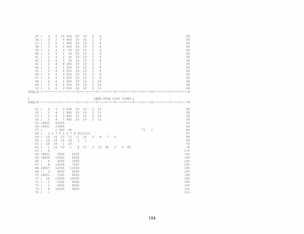
35 : 3 2 10 460 20 10 2 3 28 36 : 3 2 9 460 20 10 2 3 28 37 : 3 2 1 460 20 10 2 4 28 38 : 3 2 2 460 20 10 2 4 28 39 : 2 4 9 30 20 10 2 5 28 40 : 2 4 1 30 20 10 2 6 28 41 : 2 4 2 30 20 10 2 6 28 42 : 2 4 3 30 20 10 2 6 28 43 : 2 4 9 200 20 10 2 7 28 44 : 2 4 1 200 20 10 2 8 28 45 : 2 4 2 200 20 10 2 8 28 46 : 2 4 3 200 20 10 2 8 28 47 : 2 4 9 500 20 10 2 9 28 48 : 2 4 1 500 20 10 2 10 28 49 : 2 4 2 500 20 10 2 10 28 50 : 2 4 3 500 20 10 2 10 28 0SEQ.# :----+----1----+----2----+----3----+----4----+----5----+----6----+----7----+----8 1 CARD FILE LIST (CONT.) 0SEQ.# :----+----1----+----2----+----3----+----4----+----5----+----6----+----7----+----8 51 : 2 4 9 940 20 10 2 11 28 52 : 2 4 1 940 20 10 2 12 28 53 : 2 4 2 940 20 10 2 12 28 54 : 2 4 3 940 20 10 2 12 28 55 :8003 63200 50 56 :8001 13400 50 57 : 1 900 60 71 1 64 58 : 1 2 3 4 5 6 7 8 9101112 67 59 : 15 14 13 12 11 10 9 8 7 6 68 60 : 16 16 16 16 3 1 69 61 : 20 16 1 20 70 62 : 1 10 73 1 4 27 3 10 45 3 4 55 74 63 : 0 170 64 :8003 3500 2000 195 65 :8004 15500 6500 195 66 : 6 4500 3500 195 67 : 8 13500 7500 195 68 :8007 16500 12000 195 69 : 3 9000 9000 195 70 :8001 1500 9000 195 71 : 10 13500 10000 195 72 : 1 2500 9000 195 73 : 2 9500 9000 195 74 : 4 10500 9000 195 75 : 1 210

184

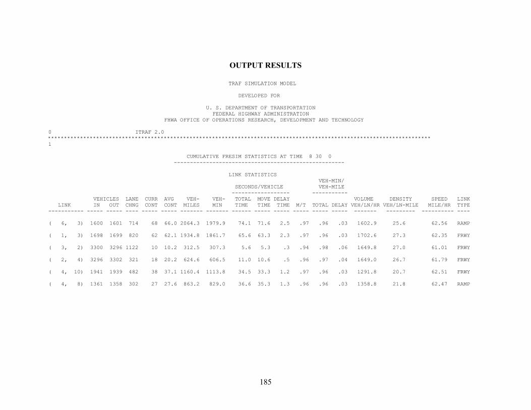
OUTPUT RESULTS

TRAF SIMULATION MODEL DEVELOPED FOR U. S. DEPARTMENT OF TRANSPORTATION FEDERAL HIGHWAY ADMINISTRATION FHWA OFFICE OF OPERATIONS RESEARCH, DEVELOPMENT AND TECHNOLOGY 0 ITRAF 2.0 *********************************************************************************************************************** 1 CUMULATIVE FRESIM STATISTICS AT TIME 8 30 0 ----------------------------------------------------- LINK STATISTICS VEH-MIN/ SECONDS/VEHICLE VEH-MILE ------------------ ----------- VEHICLES LANE CURR AVG VEH- VEH- TOTAL MOVE DELAY VOLUME DENSITY SPEED LINK LINK IN OUT CHNG CONT CONT MILES MIN TIME TIME TIME M/T TOTAL DELAY VEH/LN/HR VEH/LN-MILE MILE/HR TYPE ----------- ----- ----- ---- ----- ----- ------- ------- ------ ----- ----- ----- ----- ----- ------- --------- ---------- ---- ( 6, 3) 1600 1601 714 68 66.0 2064.3 1979.9 74.1 71.6 2.5 .97 .96 .03 1602.9 25.6 62.56 RAMP ( 1, 3) 1698 1699 820 62 62.1 1934.8 1861.7 65.6 63.3 2.3 .97 .96 .03 1702.6 27.3 62.35 FRWY ( 3, 2) 3300 3296 1122 10 10.2 312.5 307.3 5.6 5.3 .3 .94 .98 .06 1649.8 27.0 61.01 FRWY ( 2, 4) 3296 3302 321 18 20.2 624.6 606.5 11.0 10.6 .5 .96 .97 .04 1649.0 26.7 61.79 FRWY ( 4, 10) 1941 1939 482 38 37.1 1160.4 1113.8 34.5 33.3 1.2 .97 .96 .03 1291.8 20.7 62.51 FRWY ( 4, 8) 1361 1358 302 27 27.6 863.2 829.0 36.6 35.3 1.3 .96 .96 .03 1358.8 21.8 62.47 RAMP

185

Type B – Volume 3 TRAF SIMULATION MODEL DEVELOPED FOR U. S. DEPARTMENT OF TRANSPORTATION FEDERAL HIGHWAY ADMINISTRATION FHWA OFFICE OF OPERATIONS RESEARCH, DEVELOPMENT AND TECHNOLOGY 1 CARD FILE LIST 0SEQ.# :----+----1----+----2----+----3----+----4----+----5----+----6----+----7----+----8 1 :ITRAF 2.0 00 2 : 1 3 : 1 1 15 7981 1 8 8 7781 7581 2 4 :1800 3 5 : 60 4 6 : 1 5 7 :8003 6 3 1 2 1 19 8 : 6 3 2 68001 2 10 19 9 :8001 1 3 0 2 1 19 10 : 1 3 2 60000 2 1 19 11 : 3 2 4 5000 2 93 500103 500 2 19 12 : 2 4 10 10000 3 93 1000 1 9 19 13 : 4 108007 31620 3 1 19 14 : 4 88004 33541 2 1 19 15 :8003 6 12265 20 16 : 6 3 12265 20 17 :8001 1 12265 20 18 : 1 3 12265 20 19 : 3 2 12265 20 20 : 2 4 12265 2500 20 21 : 4 10 12265 20 22 : 4 8 12265 20 23 :8003 6 33500 25 24 : 6 3 23500 25 25 :8001 1 33700 25 26 : 1 3 23700 25 27 : 3 2 47200 25 28 : 2 4 104200 83000 25 29 : 4 1080074200 25 30 : 4 880043000 25 31 : 3 2 10 30 20 10 2 1 28 32 : 3 2 9 30 20 10 2 1 28 33 : 3 2 1 30 20 10 2 2 28 34 : 3 2 2 30 20 10 2 2 28

186

35 : 3 2 10 460 20 10 2 3 28 36 : 3 2 9 460 20 10 2 3 28 37 : 3 2 1 460 20 10 2 4 28 38 : 3 2 2 460 20 10 2 4 28 39 : 2 4 9 30 20 10 2 5 28 40 : 2 4 1 30 20 10 2 6 28 41 : 2 4 2 30 20 10 2 6 28 42 : 2 4 3 30 20 10 2 6 28 43 : 2 4 9 200 20 10 2 7 28 44 : 2 4 1 200 20 10 2 8 28 45 : 2 4 2 200 20 10 2 8 28 46 : 2 4 3 200 20 10 2 8 28 47 : 2 4 9 500 20 10 2 9 28 48 : 2 4 1 500 20 10 2 10 28 49 : 2 4 2 500 20 10 2 10 28 50 : 2 4 3 500 20 10 2 10 28 0SEQ.# :----+----1----+----2----+----3----+----4----+----5----+----6----+----7----+----8 1 CARD FILE LIST (CONT.) 0SEQ.# :----+----1----+----2----+----3----+----4----+----5----+----6----+----7----+----8 51 : 2 4 9 940 20 10 2 11 28 52 : 2 4 1 940 20 10 2 12 28 53 : 2 4 2 940 20 10 2 12 28 54 : 2 4 3 940 20 10 2 12 28 55 :8003 63500 50 56 :8001 13700 50 57 : 1 900 60 71 1 64 58 : 1 2 3 4 5 6 7 8 9101112 67 59 : 15 14 13 12 11 10 9 8 7 6 68 60 : 16 16 16 16 3 1 69 61 : 20 16 1 20 70 62 : 1 10 73 1 4 27 3 10 45 3 4 55 74 63 : 0 170 64 :8003 3500 2000 195 65 :8004 15500 6500 195 66 : 6 4500 3500 195 67 : 8 13500 7500 195 68 :8007 16500 12000 195 69 : 3 9000 9000 195 70 :8001 1500 9000 195 71 : 10 13500 10000 195 72 : 1 2500 9000 195 73 : 2 9500 9000 195 74 : 4 10500 9000 195 75 : 1 210

187

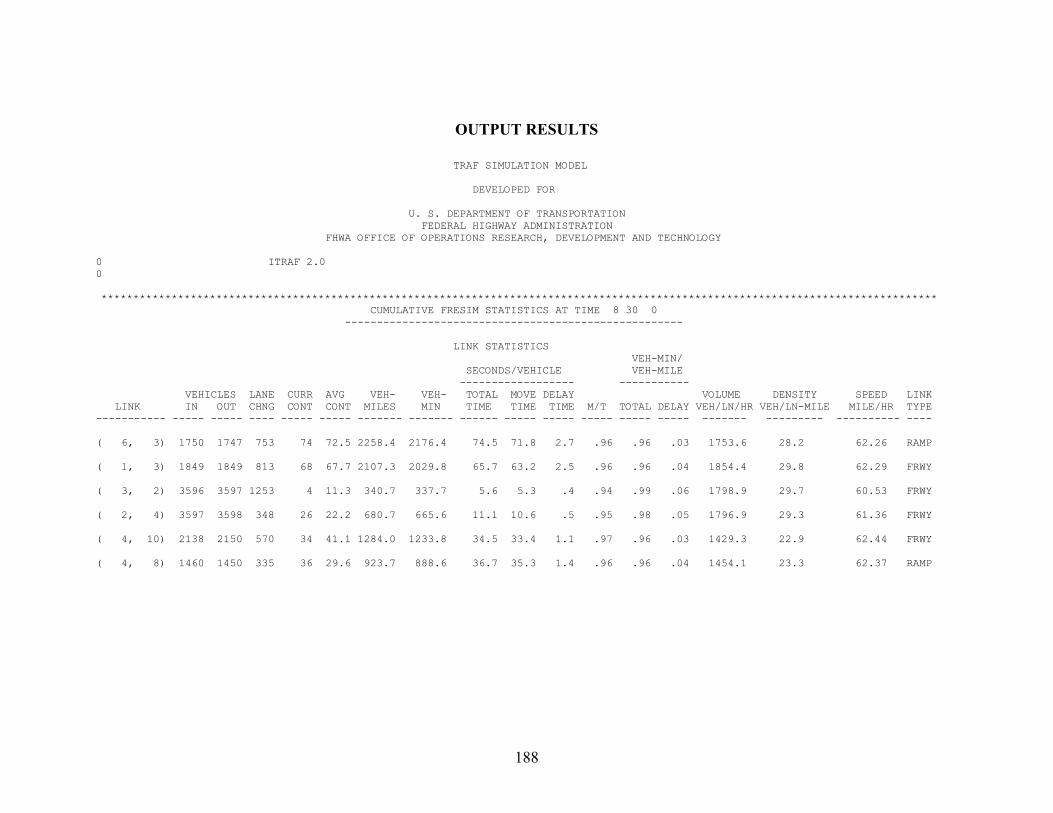
OUTPUT RESULTS TRAF SIMULATION MODEL DEVELOPED FOR U. S. DEPARTMENT OF TRANSPORTATION FEDERAL HIGHWAY ADMINISTRATION FHWA OFFICE OF OPERATIONS RESEARCH, DEVELOPMENT AND TECHNOLOGY 0 ITRAF 2.0 0 *********************************************************************************************************************************** CUMULATIVE FRESIM STATISTICS AT TIME 8 30 0 ----------------------------------------------------- LINK STATISTICS VEH-MIN/ SECONDS/VEHICLE VEH-MILE ------------------ ----------- VEHICLES LANE CURR AVG VEH- VEH- TOTAL MOVE DELAY VOLUME DENSITY SPEED LINK LINK IN OUT CHNG CONT CONT MILES MIN TIME TIME TIME M/T TOTAL DELAY VEH/LN/HR VEH/LN-MILE MILE/HR TYPE ----------- ----- ----- ---- ----- ----- ------- ------- ------ ----- ----- ----- ----- ----- ------- --------- ---------- ---- ( 6, 3) 1750 1747 753 74 72.5 2258.4 2176.4 74.5 71.8 2.7 .96 .96 .03 1753.6 28.2 62.26 RAMP ( 1, 3) 1849 1849 813 68 67.7 2107.3 2029.8 65.7 63.2 2.5 .96 .96 .04 1854.4 29.8 62.29 FRWY ( 3, 2) 3596 3597 1253 4 11.3 340.7 337.7 5.6 5.3 .4 .94 .99 .06 1798.9 29.7 60.53 FRWY ( 2, 4) 3597 3598 348 26 22.2 680.7 665.6 11.1 10.6 .5 .95 .98 .05 1796.9 29.3 61.36 FRWY ( 4, 10) 2138 2150 570 34 41.1 1284.0 1233.8 34.5 33.4 1.1 .97 .96 .03 1429.3 22.9 62.44 FRWY ( 4, 8) 1460 1450 335 36 29.6 923.7 888.6 36.7 35.3 1.4 .96 .96 .04 1454.1 23.3 62.37 RAMP

188

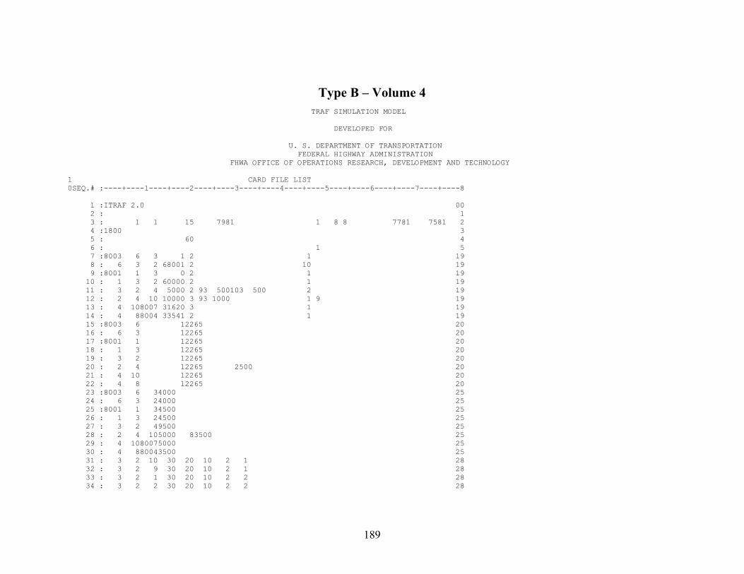
Type B – Volume 4 TRAF SIMULATION MODEL DEVELOPED FOR U. S. DEPARTMENT OF TRANSPORTATION FEDERAL HIGHWAY ADMINISTRATION FHWA OFFICE OF OPERATIONS RESEARCH, DEVELOPMENT AND TECHNOLOGY 1 CARD FILE LIST 0SEQ.# :----+----1----+----2----+----3----+----4----+----5----+----6----+----7----+----8 1 :ITRAF 2.0 00 2 : 1 3 : 1 1 15 7981 1 8 8 7781 7581 2 4 :1800 3 5 : 60 4 6 : 1 5 7 :8003 6 3 1 2 1 19 8 : 6 3 2 68001 2 10 19 9 :8001 1 3 0 2 1 19 10 : 1 3 2 60000 2 1 19 11 : 3 2 4 5000 2 93 500103 500 2 19 12 : 2 4 10 10000 3 93 1000 1 9 19 13 : 4 108007 31620 3 1 19 14 : 4 88004 33541 2 1 19 15 :8003 6 12265 20 16 : 6 3 12265 20 17 :8001 1 12265 20 18 : 1 3 12265 20 19 : 3 2 12265 20 20 : 2 4 12265 2500 20 21 : 4 10 12265 20 22 : 4 8 12265 20 23 :8003 6 34000 25 24 : 6 3 24000 25 25 :8001 1 34500 25 26 : 1 3 24500 25 27 : 3 2 49500 25 28 : 2 4 105000 83500 25 29 : 4 1080075000 25 30 : 4 880043500 25 31 : 3 2 10 30 20 10 2 1 28 32 : 3 2 9 30 20 10 2 1 28 33 : 3 2 1 30 20 10 2 2 28 34 : 3 2 2 30 20 10 2 2 28

189

35 : 3 2 10 460 20 10 2 3 28 36 : 3 2 9 460 20 10 2 3 28 37 : 3 2 1 460 20 10 2 4 28 38 : 3 2 2 460 20 10 2 4 28 39 : 2 4 9 30 20 10 2 5 28 40 : 2 4 1 30 20 10 2 6 28 41 : 2 4 2 30 20 10 2 6 28 42 : 2 4 3 30 20 10 2 6 28 43 : 2 4 9 200 20 10 2 7 28 44 : 2 4 1 200 20 10 2 8 28 45 : 2 4 2 200 20 10 2 8 28 46 : 2 4 3 200 20 10 2 8 28 47 : 2 4 9 500 20 10 2 9 28 48 : 2 4 1 500 20 10 2 10 28 49 : 2 4 2 500 20 10 2 10 28 50 : 2 4 3 500 20 10 2 10 28 0SEQ.# :----+----1----+----2----+----3----+----4----+----5----+----6----+----7----+----8 1 CARD FILE LIST (CONT.) 0SEQ.# :----+----1----+----2----+----3----+----4----+----5----+----6----+----7----+----8 51 : 2 4 9 940 20 10 2 11 28 52 : 2 4 1 940 20 10 2 12 28 53 : 2 4 2 940 20 10 2 12 28 54 : 2 4 3 940 20 10 2 12 28 55 :8003 64000 50 56 :8001 14500 50 57 : 1 900 60 71 1 64 58 : 1 2 3 4 5 6 7 8 9101112 67 59 : 15 14 13 12 11 10 9 8 7 6 68 60 : 16 16 16 16 3 1 69 61 : 20 16 1 20 70 62 : 1 10 73 1 4 27 3 10 45 3 4 55 74 63 : 0 170 64 :8003 3500 2000 195 65 :8004 15500 6500 195 66 : 6 4500 3500 195 67 : 8 13500 7500 195 68 :8007 16500 12000 195 69 : 3 9000 9000 195 70 :8001 1500 9000 195 71 : 10 13500 10000 195 72 : 1 2500 9000 195 73 : 2 9500 9000 195 74 : 4 10500 9000 195 75 : 1 210

190

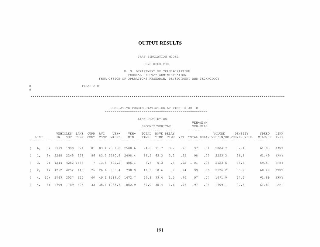
OUTPUT RESULTS

TRAF SIMULATION MODEL DEVELOPED FOR U. S. DEPARTMENT OF TRANSPORTATION FEDERAL HIGHWAY ADMINISTRATION FHWA OFFICE OF OPERATIONS RESEARCH, DEVELOPMENT AND TECHNOLOGY 0 ITRAF 2.0 0 *********************************************************************************************************************************** CUMULATIVE FRESIM STATISTICS AT TIME 8 30 0 ----------------------------------------------------- LINK STATISTICS VEH-MIN/ SECONDS/VEHICLE VEH-MILE ------------------ ----------- VEHICLES LANE CURR AVG VEH- VEH- TOTAL MOVE DELAY VOLUME DENSITY SPEED LINK LINK IN OUT CHNG CONT CONT MILES MIN TIME TIME TIME M/T TOTAL DELAY VEH/LN/HR VEH/LN-MILE MILE/HR TYPE ----------- ----- ----- ---- ----- ----- ------- ------- ------ ----- ----- ----- ----- ----- ------- --------- ---------- ---- ( 6, 3) 1999 1999 824 81 83.4 2581.8 2500.6 74.8 71.7 3.2 .96 .97 .04 2004.7 32.4 61.95 RAMP ( 1, 3) 2248 2245 953 86 83.3 2560.6 2498.4 66.5 63.3 3.2 .95 .98 .05 2253.3 36.6 61.49 FRWY ( 3, 2) 4244 4252 1456 7 13.5 402.2 405.1 5.7 5.3 .5 .92 1.01 .08 2123.5 35.6 59.57 FRWY ( 2, 4) 4252 4252 445 26 26.6 805.4 798.9 11.3 10.6 .7 .94 .99 .06 2126.2 35.2 60.49 FRWY ( 4, 10) 2543 2527 634 60 49.1 1519.0 1472.7 34.8 33.4 1.5 .96 .97 .04 1691.0 27.3 61.89 FRWY ( 4, 8) 1709 1709 406 33 35.1 1085.7 1052.9 37.0 35.4 1.6 .96 .97 .04 1709.1 27.6 61.87 RAMP

191

Type B – Volume 5 TRAF SIMULATION MODEL DEVELOPED FOR U. S. DEPARTMENT OF TRANSPORTATION FEDERAL HIGHWAY ADMINISTRATION FHWA OFFICE OF OPERATIONS RESEARCH, DEVELOPMENT AND TECHNOLOGY 1 CARD FILE LIST 0SEQ.# :----+----1----+----2----+----3----+----4----+----5----+----6----+----7----+----8 1 :ITRAF 2.0 00 2 : 1 3 : 1 1 15 7981 1 8 8 7781 7581 2 4 :1800 3 5 : 60 4 6 : 1 5 7 :8003 6 3 1 2 1 19 8 : 6 3 2 68001 2 10 19 9 :8001 1 3 0 2 1 19 10 : 1 3 2 60000 2 1 19 11 : 3 2 4 5000 2 93 500103 500 2 19 12 : 2 4 10 10000 3 93 1000 1 9 19 13 : 4 108007 31620 3 1 19 14 : 4 88004 33541 2 1 19 15 :8003 6 12265 20 16 : 6 3 12265 20 17 :8001 1 12265 20 18 : 1 3 12265 20 19 : 3 2 12265 20 20 : 2 4 12265 2500 20 21 : 4 10 12265 20 22 : 4 8 12265 20 23 :8003 6 33500 25 24 : 6 3 23500 25 25 :8001 1 33800 25 26 : 1 3 23800 25 27 : 3 2 47300 25 28 : 2 4 103500 83800 25 29 : 4 1080073500 25 30 : 4 880043800 25 31 : 3 2 10 30 20 10 2 1 28 32 : 3 2 9 30 20 10 2 1 28 33 : 3 2 1 30 20 10 2 2 28 34 : 3 2 2 30 20 10 2 2 28

192

35 : 3 2 10 460 20 10 2 3 28 36 : 3 2 9 460 20 10 2 3 28 37 : 3 2 1 460 20 10 2 4 28 38 : 3 2 2 460 20 10 2 4 28 39 : 2 4 9 30 20 10 2 5 28 40 : 2 4 1 30 20 10 2 6 28 41 : 2 4 2 30 20 10 2 6 28 42 : 2 4 3 30 20 10 2 6 28 43 : 2 4 9 200 20 10 2 7 28 44 : 2 4 1 200 20 10 2 8 28 45 : 2 4 2 200 20 10 2 8 28 46 : 2 4 3 200 20 10 2 8 28 47 : 2 4 9 500 20 10 2 9 28 48 : 2 4 1 500 20 10 2 10 28 49 : 2 4 2 500 20 10 2 10 28 50 : 2 4 3 500 20 10 2 10 28 0SEQ.# :----+----1----+----2----+----3----+----4----+----5----+----6----+----7----+----8 1 CARD FILE LIST (CONT.) 0SEQ.# :----+----1----+----2----+----3----+----4----+----5----+----6----+----7----+----8 51 : 2 4 9 940 20 10 2 11 28 52 : 2 4 1 940 20 10 2 12 28 53 : 2 4 2 940 20 10 2 12 28 54 : 2 4 3 940 20 10 2 12 28 55 :8003 63500 50 56 :8001 13800 50 57 : 1 900 60 71 1 64 58 : 1 2 3 4 5 6 7 8 9101112 67 59 : 15 14 13 12 11 10 9 8 7 6 68 60 : 16 16 16 16 3 1 69 61 : 20 16 1 20 70 62 : 1 10 73 1 4 27 3 10 45 3 4 55 74 63 : 0 170 64 :8003 3500 2000 195 65 :8004 15500 6500 195 66 : 6 4500 3500 195 67 : 8 13500 7500 195 68 :8007 16500 12000 195 69 : 3 9000 9000 195 70 :8001 1500 9000 195 71 : 10 13500 10000 195 72 : 1 2500 9000 195 73 : 2 9500 9000 195 74 : 4 10500 9000 195 75 : 1 210

193

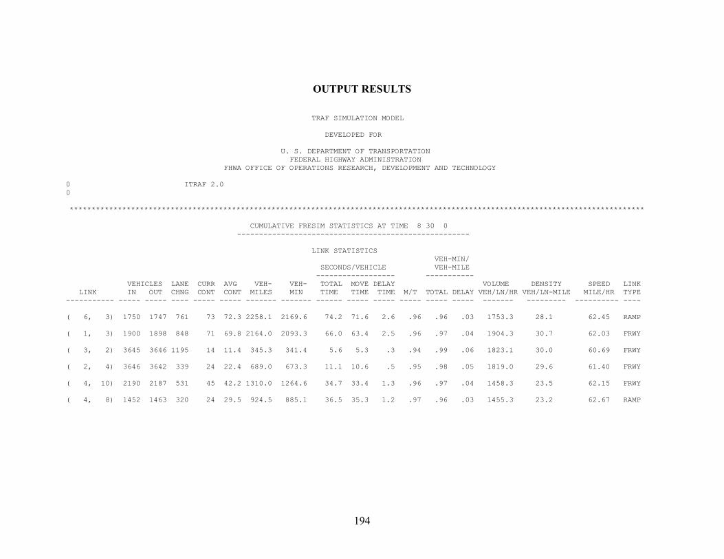
OUTPUT RESULTS

TRAF SIMULATION MODEL DEVELOPED FOR U. S. DEPARTMENT OF TRANSPORTATION FEDERAL HIGHWAY ADMINISTRATION FHWA OFFICE OF OPERATIONS RESEARCH, DEVELOPMENT AND TECHNOLOGY 0 ITRAF 2.0 0 *********************************************************************************************************************************** CUMULATIVE FRESIM STATISTICS AT TIME 8 30 0 ----------------------------------------------------- LINK STATISTICS VEH-MIN/ SECONDS/VEHICLE VEH-MILE ------------------ ----------- VEHICLES LANE CURR AVG VEH- VEH- TOTAL MOVE DELAY VOLUME DENSITY SPEED LINK LINK IN OUT CHNG CONT CONT MILES MIN TIME TIME TIME M/T TOTAL DELAY VEH/LN/HR VEH/LN-MILE MILE/HR TYPE ----------- ----- ----- ---- ----- ----- ------- ------- ------ ----- ----- ----- ----- ----- ------- --------- ---------- ---- ( 6, 3) 1750 1747 761 73 72.3 2258.1 2169.6 74.2 71.6 2.6 .96 .96 .03 1753.3 28.1 62.45 RAMP ( 1, 3) 1900 1898 848 71 69.8 2164.0 2093.3 66.0 63.4 2.5 .96 .97 .04 1904.3 30.7 62.03 FRWY ( 3, 2) 3645 3646 1195 14 11.4 345.3 341.4 5.6 5.3 .3 .94 .99 .06 1823.1 30.0 60.69 FRWY ( 2, 4) 3646 3642 339 24 22.4 689.0 673.3 11.1 10.6 .5 .95 .98 .05 1819.0 29.6 61.40 FRWY ( 4, 10) 2190 2187 531 45 42.2 1310.0 1264.6 34.7 33.4 1.3 .96 .97 .04 1458.3 23.5 62.15 FRWY ( 4, 8) 1452 1463 320 24 29.5 924.5 885.1 36.5 35.3 1.2 .97 .96 .03 1455.3 23.2 62.67 RAMP

194

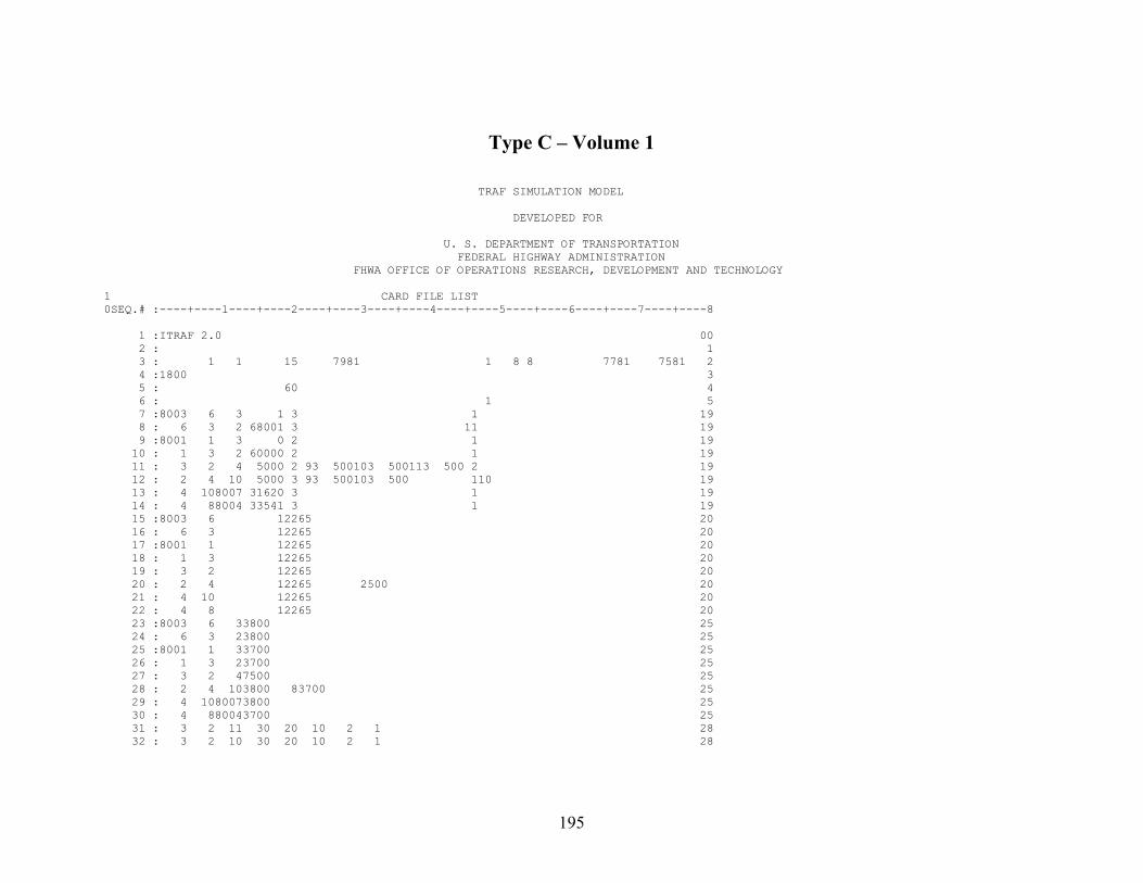
Type C – Volume 1 TRAF SIMULATION MODEL DEVELOPED FOR U. S. DEPARTMENT OF TRANSPORTATION FEDERAL HIGHWAY ADMINISTRATION FHWA OFFICE OF OPERATIONS RESEARCH, DEVELOPMENT AND TECHNOLOGY 1 CARD FILE LIST 0SEQ.# :----+----1----+----2----+----3----+----4----+----5----+----6----+----7----+----8 1 :ITRAF 2.0 00 2 : 1 3 : 1 1 15 7981 1 8 8 7781 7581 2 4 :1800 3 5 : 60 4 6 : 1 5 7 :8003 6 3 1 3 1 19 8 : 6 3 2 68001 3 11 19 9 :8001 1 3 0 2 1 19 10 : 1 3 2 60000 2 1 19 11 : 3 2 4 5000 2 93 500103 500113 500 2 19 12 : 2 4 10 5000 3 93 500103 500 110 19 13 : 4 108007 31620 3 1 19 14 : 4 88004 33541 3 1 19 15 :8003 6 12265 20 16 : 6 3 12265 20 17 :8001 1 12265 20 18 : 1 3 12265 20 19 : 3 2 12265 20 20 : 2 4 12265 2500 20 21 : 4 10 12265 20 22 : 4 8 12265 20 23 :8003 6 33800 25 24 : 6 3 23800 25 25 :8001 1 33700 25 26 : 1 3 23700 25 27 : 3 2 47500 25 28 : 2 4 103800 83700 25 29 : 4 1080073800 25 30 : 4 880043700 25 31 : 3 2 11 30 20 10 2 1 28 32 : 3 2 10 30 20 10 2 1 28

195

33 : 3 2 9 30 20 10 2 1 28 34 : 3 2 1 30 20 10 2 2 28 35 : 3 2 2 30 20 10 2 2 28 36 : 3 2 11 200 20 10 2 3 28 37 : 3 2 10 200 20 10 2 3 28 38 : 3 2 9 200 20 10 2 3 28 39 : 3 2 1 200 20 10 2 4 28 40 : 3 2 2 200 20 10 2 4 28 41 : 3 2 11 460 20 10 2 5 28 42 : 3 2 10 460 20 10 2 5 28 43 : 3 2 9 460 20 10 2 5 28 44 : 3 2 1 460 20 10 2 6 28 45 : 3 2 2 460 20 10 2 6 28 46 : 2 4 10 30 20 10 2 7 28 47 : 2 4 9 30 20 10 2 7 28 48 : 2 4 1 30 20 10 2 8 28 49 : 2 4 2 30 20 10 2 8 28 50 : 2 4 3 30 20 10 2 8 28 0SEQ.# :----+----1----+----2----+----3----+----4----+----5----+----6----+----7----+----8 1 CARD FILE LIST (CONT.) 0SEQ.# :----+----1----+----2----+----3----+----4----+----5----+----6----+----7----+----8 51 : 2 4 10 200 20 10 2 9 28 52 : 2 4 9 200 20 10 2 9 28 53 : 2 4 1 200 20 10 2 10 28 54 : 2 4 2 200 20 10 2 10 28 55 : 2 4 3 200 20 10 2 10 28 56 : 2 4 10 460 20 10 2 11 28 57 : 2 4 9 460 20 10 2 11 28 58 : 2 4 1 460 20 10 2 12 28 59 : 2 4 2 460 20 10 2 12 28 60 : 2 4 3 460 20 10 2 12 28 61 :8003 63800 50 62 :8001 13700 50 63 : 1 900 60 71 1 64 64 : 1 2 3 4 5 6 7 8 9101112 67 65 : 15 14 13 12 11 10 9 8 7 6 68 66 : 16 16 16 16 3 1 69 67 : 20 16 1 20 70 68 : 1 10 73 1 4 27 3 10 45 3 4 55 74 69 : 0 170 70 :8003 3500 2000 195 71 :8004 15000 6500 195 72 : 6 4500 3500 195 73 : 8 13000 7500 195 74 :8007 16000 12000 195

196

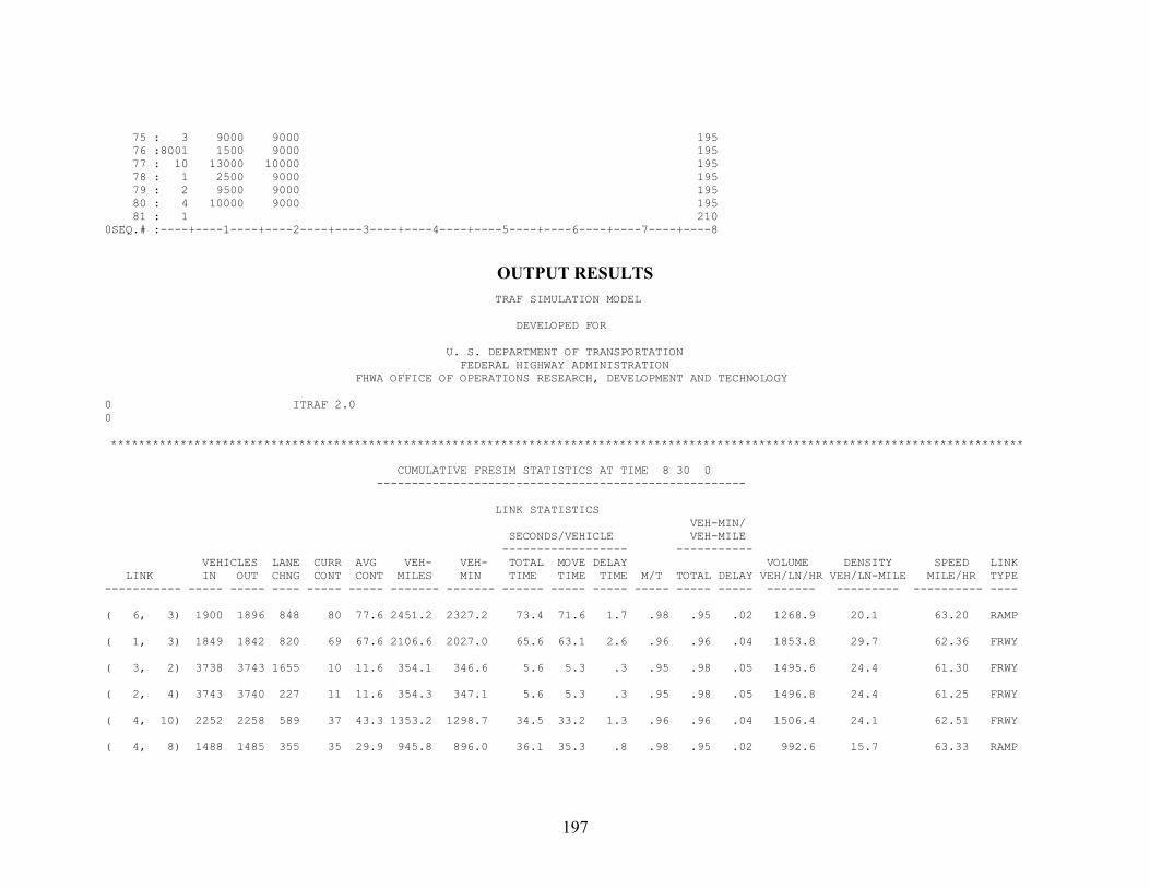
75 : 3 9000 9000 195 76 :8001 1500 9000 195 77 : 10 13000 10000 195 78 : 1 2500 9000 195 79 : 2 9500 9000 195 80 : 4 10000 9000 195 81 : 1 210 0SEQ.# :----+----1----+----2----+----3----+----4----+----5----+----6----+----7----+----8

OUTPUT RESULTS TRAF SIMULATION MODEL DEVELOPED FOR U. S. DEPARTMENT OF TRANSPORTATION FEDERAL HIGHWAY ADMINISTRATION FHWA OFFICE OF OPERATIONS RESEARCH, DEVELOPMENT AND TECHNOLOGY 0 ITRAF 2.0 0 *********************************************************************************************************************************** CUMULATIVE FRESIM STATISTICS AT TIME 8 30 0 ----------------------------------------------------- LINK STATISTICS VEH-MIN/ SECONDS/VEHICLE VEH-MILE ------------------ ----------- VEHICLES LANE CURR AVG VEH- VEH- TOTAL MOVE DELAY VOLUME DENSITY SPEED LINK LINK IN OUT CHNG CONT CONT MILES MIN TIME TIME TIME M/T TOTAL DELAY VEH/LN/HR VEH/LN-MILE MILE/HR TYPE ----------- ----- ----- ---- ----- ----- ------- ------- ------ ----- ----- ----- ----- ----- ------- --------- ---------- ---- ( 6, 3) 1900 1896 848 80 77.6 2451.2 2327.2 73.4 71.6 1.7 .98 .95 .02 1268.9 20.1 63.20 RAMP ( 1, 3) 1849 1842 820 69 67.6 2106.6 2027.0 65.6 63.1 2.6 .96 .96 .04 1853.8 29.7 62.36 FRWY ( 3, 2) 3738 3743 1655 10 11.6 354.1 346.6 5.6 5.3 .3 .95 .98 .05 1495.6 24.4 61.30 FRWY ( 2, 4) 3743 3740 227 11 11.6 354.3 347.1 5.6 5.3 .3 .95 .98 .05 1496.8 24.4 61.25 FRWY ( 4, 10) 2252 2258 589 37 43.3 1353.2 1298.7 34.5 33.2 1.3 .96 .96 .04 1506.4 24.1 62.51 FRWY ( 4, 8) 1488 1485 355 35 29.9 945.8 896.0 36.1 35.3 .8 .98 .95 .02 992.6 15.7 63.33 RAMP

197

Type C – Volume 2 TRAF SIMULATION MODEL DEVELOPED FOR U. S. DEPARTMENT OF TRANSPORTATION FEDERAL HIGHWAY ADMINISTRATION FHWA OFFICE OF OPERATIONS RESEARCH, DEVELOPMENT AND TECHNOLOGY 1 CARD FILE LIST 0SEQ.# :----+----1----+----2----+----3----+----4----+----5----+----6----+----7----+----8 1 :ITRAF 2.0 00 2 : 1 3 : 1 1 15 7981 1 8 8 7781 7581 2 4 :1800 3 5 : 60 4 6 : 1 5 7 :8003 6 3 1 3 1 19 8 : 6 3 2 68001 3 11 19 9 :8001 1 3 0 2 1 19 10 : 1 3 2 60000 2 1 19 11 : 3 2 4 5000 2 93 500103 500113 500 2 19 12 : 2 4 10 5000 3 93 500103 500 110 19 13 : 4 108007 31620 3 1 19 14 : 4 88004 33541 3 1 19 15 :8003 6 12265 20 16 : 6 3 12265 20 17 :8001 1 12265 20 18 : 1 3 12265 20 19 : 3 2 12265 20 20 : 2 4 12265 2500 20 21 : 4 10 12265 20 22 : 4 8 12265 20 23 :8003 6 34350 25 24 : 6 3 24350 25 25 :8001 1 34300 25 26 : 1 3 24300 25 27 : 3 2 48650 25 28 : 2 4 104350 84300 25 29 : 4 1080074350 25 30 : 4 880044300 25 31 : 3 2 11 30 20 10 2 1 28 32 : 3 2 10 30 20 10 2 1 28

198

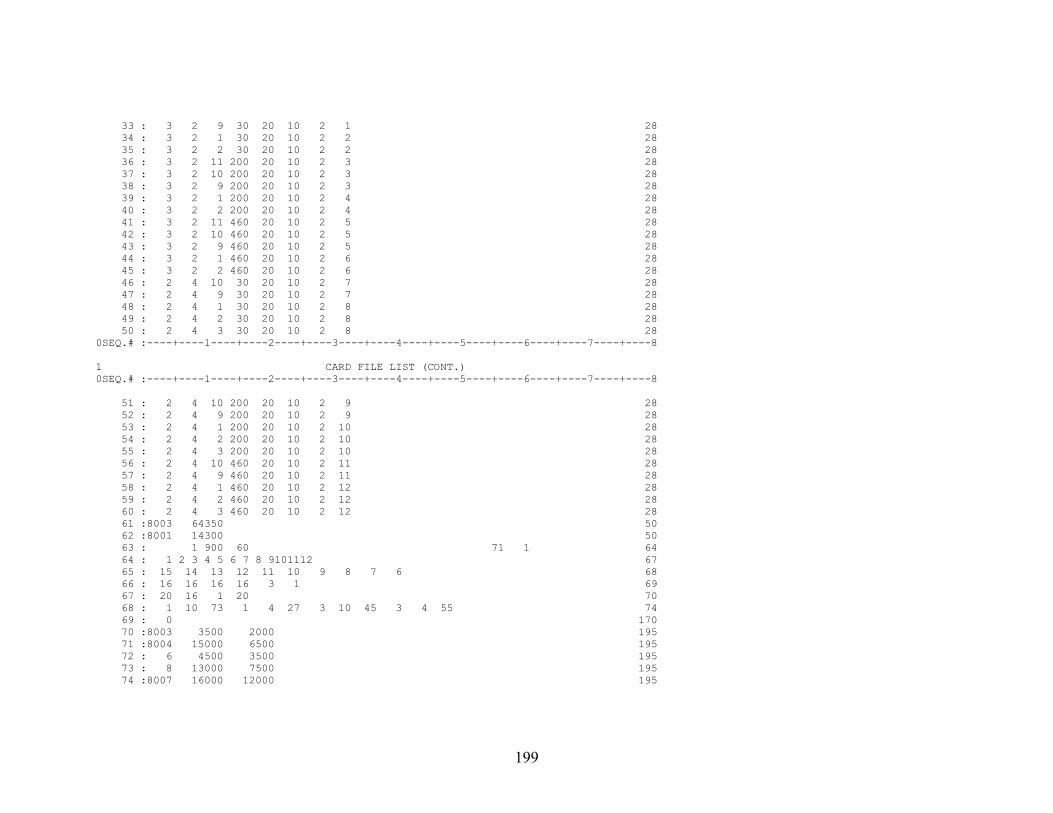
33 : 3 2 9 30 20 10 2 1 28 34 : 3 2 1 30 20 10 2 2 28 35 : 3 2 2 30 20 10 2 2 28 36 : 3 2 11 200 20 10 2 3 28 37 : 3 2 10 200 20 10 2 3 28 38 : 3 2 9 200 20 10 2 3 28 39 : 3 2 1 200 20 10 2 4 28 40 : 3 2 2 200 20 10 2 4 28 41 : 3 2 11 460 20 10 2 5 28 42 : 3 2 10 460 20 10 2 5 28 43 : 3 2 9 460 20 10 2 5 28 44 : 3 2 1 460 20 10 2 6 28 45 : 3 2 2 460 20 10 2 6 28 46 : 2 4 10 30 20 10 2 7 28 47 : 2 4 9 30 20 10 2 7 28 48 : 2 4 1 30 20 10 2 8 28 49 : 2 4 2 30 20 10 2 8 28 50 : 2 4 3 30 20 10 2 8 28 0SEQ.# :----+----1----+----2----+----3----+----4----+----5----+----6----+----7----+----8 1 CARD FILE LIST (CONT.) 0SEQ.# :----+----1----+----2----+----3----+----4----+----5----+----6----+----7----+----8 51 : 2 4 10 200 20 10 2 9 28 52 : 2 4 9 200 20 10 2 9 28 53 : 2 4 1 200 20 10 2 10 28 54 : 2 4 2 200 20 10 2 10 28 55 : 2 4 3 200 20 10 2 10 28 56 : 2 4 10 460 20 10 2 11 28 57 : 2 4 9 460 20 10 2 11 28 58 : 2 4 1 460 20 10 2 12 28 59 : 2 4 2 460 20 10 2 12 28 60 : 2 4 3 460 20 10 2 12 28 61 :8003 64350 50 62 :8001 14300 50 63 : 1 900 60 71 1 64 64 : 1 2 3 4 5 6 7 8 9101112 67 65 : 15 14 13 12 11 10 9 8 7 6 68 66 : 16 16 16 16 3 1 69 67 : 20 16 1 20 70 68 : 1 10 73 1 4 27 3 10 45 3 4 55 74 69 : 0 170 70 :8003 3500 2000 195 71 :8004 15000 6500 195 72 : 6 4500 3500 195 73 : 8 13000 7500 195 74 :8007 16000 12000 195

199

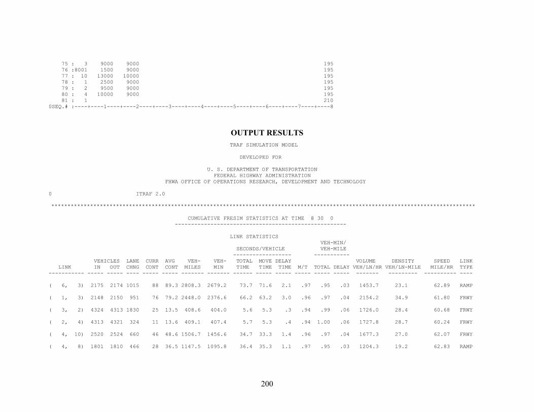
75 : 3 9000 9000 195 76 :8001 1500 9000 195 77 : 10 13000 10000 195 78 : 1 2500 9000 195 79 : 2 9500 9000 195 80 : 4 10000 9000 195 81 : 1 210 0SEQ.# :----+----1----+----2----+----3----+----4----+----5----+----6----+----7----+----8

OUTPUT RESULTS TRAF SIMULATION MODEL DEVELOPED FOR U. S. DEPARTMENT OF TRANSPORTATION

***********************************************************************************************************************************

FEDERAL HIGHWAY ADMINISTRATION FHWA OFFICE OF OPERATIONS RESEARCH, DEVELOPMENT AND TECHNOLOGY 0 ITRAF 2.0

CUMULATIVE FRESIM STATISTICS AT TIME 8 30 0 ----------------------------------------------------- LINK STATISTICS VEH-MIN/ SECONDS/VEHICLE VEH-MILE ------------------ ----------- VEHICLES LANE CURR AVG VEH- VEH- TOTAL MOVE DELAY VOLUME DENSITY SPEED LINK LINK IN OUT CHNG CONT CONT MILES MIN TIME TIME TIME M/T TOTAL DELAY VEH/LN/HR VEH/LN-MILE MILE/HR TYPE ----------- ----- ----- ---- ----- ----- ------- ------- ------ ----- ----- ----- ----- ----- ------- --------- ---------- ---- ( 6, 3) 2175 2174 1015 88 89.3 2808.3 2679.2 73.7 71.6 2.1 .97 .95 .03 1453.7 23.1 62.89 RAMP ( 1, 3) 2148 2150 951 76 79.2 2448.0 2376.6 66.2 63.2 3.0 .96 .97 .04 2154.2 34.9 61.80 FRWY ( 3, 2) 4324 4313 1830 25 13.5 408.6 404.0 5.6 5.3 .3 .94 .99 .06 1726.0 28.4 60.68 FRWY ( 2, 4) 4313 4321 324 11 13.6 409.1 407.4 5.7 5.3 .4 .94 1.00 .06 1727.8 28.7 60.24 FRWY ( 4, 10) 2520 2524 660 46 48.6 1506.7 1456.6 34.7 33.3 1.4 .96 .97 .04 1677.3 27.0 62.07 FRWY ( 4, 8) 1801 1810 466 28 36.5 1147.5 1095.8 36.4 35.3 1.1 .97 .95 .03 1204.3 19.2 62.83 RAMP

200

Type C – Volume 3 TRAF SIMULATION MODEL DEVELOPED FOR U. S. DEPARTMENT OF TRANSPORTATION FEDERAL HIGHWAY ADMINISTRATION FHWA OFFICE OF OPERATIONS RESEARCH, DEVELOPMENT AND TECHNOLOGY 1 CARD FILE LIST 0SEQ.# :----+----1----+----2----+----3----+----4----+----5----+----6----+----7----+----8 1 :ITRAF 2.0 00 2 : 1 3 : 1 1 15 7981 1 8 8 7781 7581 2 4 :1800 3 5 : 60 4 6 : 1 5 7 :8003 6 3 1 3 1 19 8 : 6 3 2 68001 3 11 19 9 :8001 1 3 0 2 1 19 10 : 1 3 2 60000 2 1 19 11 : 3 2 4 5000 2 93 500103 500113 500 2 19 12 : 2 4 10 5000 3 93 500103 500 110 19 13 : 4 108007 31620 3 1 19 14 : 4 88004 33541 3 1 19 15 :8003 6 12265 20 16 : 6 3 12265 20 17 :8001 1 12265 20 18 : 1 3 12265 20 19 : 3 2 12265 20 20 : 2 4 12265 2500 20 21 : 4 10 12265 20 22 : 4 8 12265 20 23 :8003 6 32100 25 24 : 6 3 22100 25 25 :8001 1 32050 25 26 : 1 3 22050 25 27 : 3 2 44150 25 28 : 2 4 102100 82050 25 29 : 4 1080072100 25 30 : 4 880042050 25 31 : 3 2 11 30 20 10 2 1 28

201

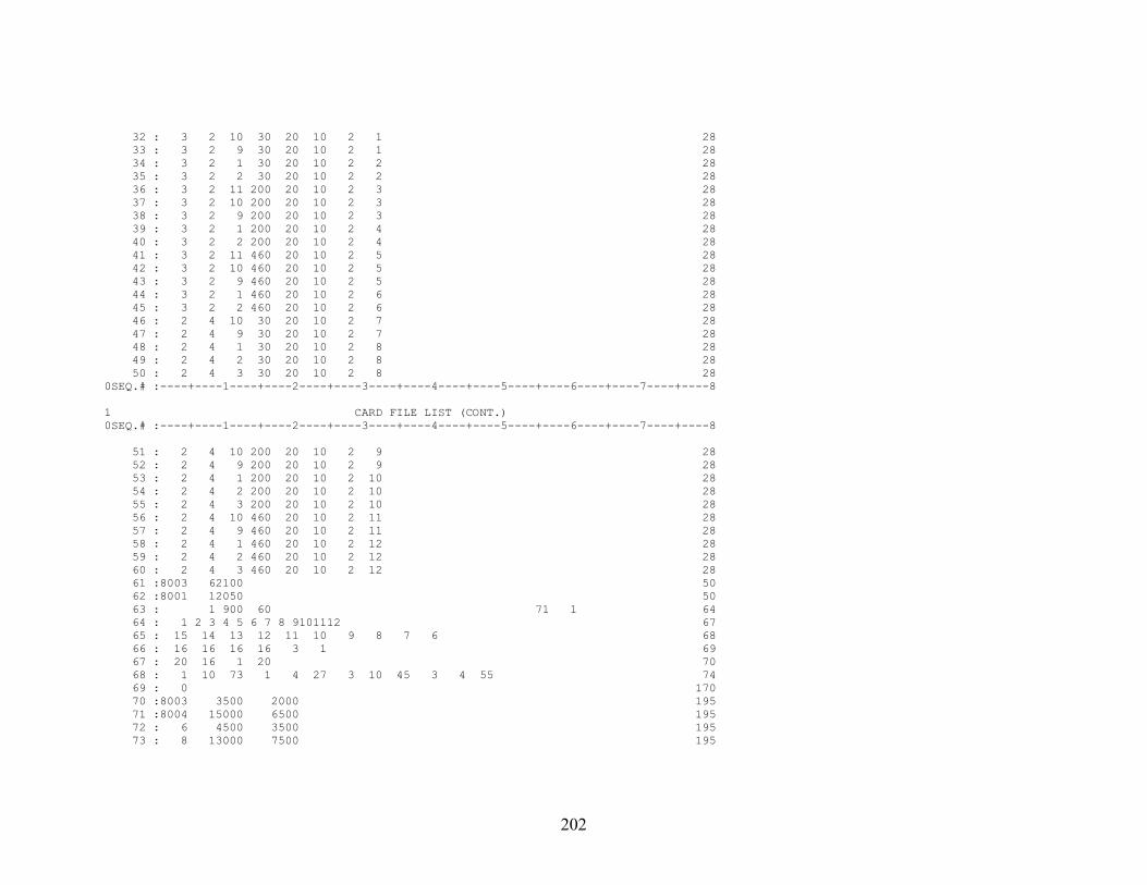
32 : 3 2 10 30 20 10 2 1 28 33 : 3 2 9 30 20 10 2 1 28 34 : 3 2 1 30 20 10 2 2 28 35 : 3 2 2 30 20 10 2 2 28 36 : 3 2 11 200 20 10 2 3 28 37 : 3 2 10 200 20 10 2 3 28 38 : 3 2 9 200 20 10 2 3 28 39 : 3 2 1 200 20 10 2 4 28 40 : 3 2 2 200 20 10 2 4 28 41 : 3 2 11 460 20 10 2 5 28 42 : 3 2 10 460 20 10 2 5 28 43 : 3 2 9 460 20 10 2 5 28 44 : 3 2 1 460 20 10 2 6 28 45 : 3 2 2 460 20 10 2 6 28 46 : 2 4 10 30 20 10 2 7 28 47 : 2 4 9 30 20 10 2 7 28 48 : 2 4 1 30 20 10 2 8 28 49 : 2 4 2 30 20 10 2 8 28 50 : 2 4 3 30 20 10 2 8 28 0SEQ.# :----+----1----+----2----+----3----+----4----+----5----+----6----+----7----+----8 1 CARD FILE LIST (CONT.) 0SEQ.# :----+----1----+----2----+----3----+----4----+----5----+----6----+----7----+----8 51 : 2 4 10 200 20 10 2 9 28 52 : 2 4 9 200 20 10 2 9 28 53 : 2 4 1 200 20 10 2 10 28 54 : 2 4 2 200 20 10 2 10 28 55 : 2 4 3 200 20 10 2 10 28 56 : 2 4 10 460 20 10 2 11 28 57 : 2 4 9 460 20 10 2 11 28 58 : 2 4 1 460 20 10 2 12 28 59 : 2 4 2 460 20 10 2 12 28 60 : 2 4 3 460 20 10 2 12 28 61 :8003 62100 50 62 :8001 12050 50 63 : 1 900 60 71 1 64 64 : 1 2 3 4 5 6 7 8 9101112 67 65 : 15 14 13 12 11 10 9 8 7 6 68 66 : 16 16 16 16 3 1 69 67 : 20 16 1 20 70 68 : 1 10 73 1 4 27 3 10 45 3 4 55 74 69 : 0 170 70 :8003 3500 2000 195 71 :8004 15000 6500 195 72 : 6 4500 3500 195 73 : 8 13000 7500 195

202

74 :8007 16000 12000 195 75 : 3 9000 9000 195 76 :8001 1500 9000 195 77 : 10 13000 10000 195 78 : 1 2500 9000 195 79 : 2 9500 9000 195 80 : 4 10000 9000 195 81 : 1 210 0SEQ.# :----+----1----+----2----+----3----+----4----+----5----+----6----+----7----+----8

OUTPUT RESULTS TRAF SIMULATION MODEL DEVELOPED FOR U. S. DEPARTMENT OF TRANSPORTATION FEDERAL HIGHWAY ADMINISTRATION FHWA OFFICE OF OPERATIONS RESEARCH, DEVELOPMENT AND TECHNOLOGY 0 ITRAF 2.0 0 *********************************************************************************************************************************** CUMULATIVE FRESIM STATISTICS AT TIME 8 30 0 ----------------------------------------------------- LINK STATISTICS VEH-MIN/ SECONDS/VEHICLE VEH-MILE ------------------ ----------- VEHICLES LANE CURR AVG VEH- VEH- TOTAL MOVE DELAY VOLUME DENSITY SPEED LINK LINK IN OUT CHNG CONT CONT MILES MIN TIME TIME TIME M/T TOTAL DELAY VEH/LN/HR VEH/LN-MILE MILE/HR TYPE ----------- ----- ----- ---- ----- ----- ------- ------- ------ ----- ----- ----- ----- ----- ------- --------- ---------- ---- ( 6, 3) 1049 1050 411 42 42.4 1354.9 1271.7 72.5 71.7 .8 .99 .94 .01 701.4 11.0 63.93 RAMP ( 1, 3) 1025 1027 465 37 36.9 1167.6 1106.4 64.6 63.5 1.1 .98 .95 .02 1027.5 16.2 63.32 FRWY ( 3, 2) 2077 2070 912 9 6.2 196.3 187.5 5.4 5.3 .1 .97 .96 .03 829.0 13.2 62.81 FRWY ( 2, 4) 2070 2070 117 6 6.3 196.1 187.6 5.4 5.3 .1 .98 .96 .02 828.3 13.2 62.72 FRWY ( 4, 10) 1216 1219 238 24 23.0 729.1 689.3 34.0 33.4 .6 .98 .95 .02 811.6 12.8 63.46 FRWY ( 4, 8) 854 854 160 16 17.0 542.3 511.1 35.9 35.4 .5 .99 .94 .01 569.2 8.9 63.67 RAMP

203

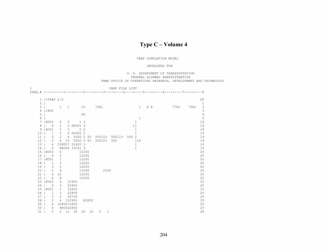
Type C – Volume 4 TRAF SIMULATION MODEL DEVELOPED FOR U. S. DEPARTMENT OF TRANSPORTATION FEDERAL HIGHWAY ADMINISTRATION FHWA OFFICE OF OPERATIONS RESEARCH, DEVELOPMENT AND TECHNOLOGY 1 CARD FILE LIST 0SEQ.# :----+----1----+----2----+----3----+----4----+----5----+----6----+----7----+----8 1 :ITRAF 2.0 00 2 : 1 3 : 1 1 15 7981 1 8 8 7781 7581 2 4 :1800 3 5 : 60 4 6 : 1 5 7 :8003 6 3 1 3 1 19 8 : 6 3 2 68001 3 11 19 9 :8001 1 3 0 2 1 19 10 : 1 3 2 60000 2 1 19 11 : 3 2 4 5000 2 93 500103 500113 500 2 19 12 : 2 4 10 5000 3 93 500103 500 110 19 13 : 4 108007 31620 3 1 19 14 : 4 88004 33541 3 1 19 15 :8003 6 12265 20 16 : 6 3 12265 20 17 :8001 1 12265 20 18 : 1 3 12265 20 19 : 3 2 12265 20 20 : 2 4 12265 2500 20 21 : 4 10 12265 20 22 : 4 8 12265 20 23 :8003 6 32900 25 24 : 6 3 22900 25 25 :8001 1 32850 25 26 : 1 3 22850 25 27 : 3 2 45750 25 28 : 2 4 102900 82850 25 29 : 4 1080072900 25 30 : 4 880042850 25 31 : 3 2 11 30 20 10 2 1 28

204

32 : 3 2 10 30 20 10 2 1 28 33 : 3 2 9 30 20 10 2 1 28 34 : 3 2 1 30 20 10 2 2 28 35 : 3 2 2 30 20 10 2 2 28 36 : 3 2 11 200 20 10 2 3 28 37 : 3 2 10 200 20 10 2 3 28 38 : 3 2 9 200 20 10 2 3 28 39 : 3 2 1 200 20 10 2 4 28 40 : 3 2 2 200 20 10 2 4 28 41 : 3 2 11 460 20 10 2 5 28 42 : 3 2 10 460 20 10 2 5 28 43 : 3 2 9 460 20 10 2 5 28 44 : 3 2 1 460 20 10 2 6 28 45 : 3 2 2 460 20 10 2 6 28 46 : 2 4 10 30 20 10 2 7 28 47 : 2 4 9 30 20 10 2 7 28 48 : 2 4 1 30 20 10 2 8 28 49 : 2 4 2 30 20 10 2 8 28 50 : 2 4 3 30 20 10 2 8 28 0SEQ.# :----+----1----+----2----+----3----+----4----+----5----+----6----+----7----+----8 1 CARD FILE LIST (CONT.) 0SEQ.# :----+----1----+----2----+----3----+----4----+----5----+----6----+----7----+----8 51 : 2 4 10 200 20 10 2 9 28 52 : 2 4 9 200 20 10 2 9 28 53 : 2 4 1 200 20 10 2 10 28 54 : 2 4 2 200 20 10 2 10 28 55 : 2 4 3 200 20 10 2 10 28 56 : 2 4 10 460 20 10 2 11 28 57 : 2 4 9 460 20 10 2 11 28 58 : 2 4 1 460 20 10 2 12 28 59 : 2 4 2 460 20 10 2 12 28 60 : 2 4 3 460 20 10 2 12 28 61 :8003 62900 50 62 :8001 12850 50 63 : 1 900 60 71 1 64 64 : 1 2 3 4 5 6 7 8 9101112 67 65 : 15 14 13 12 11 10 9 8 7 6 68 66 : 16 16 16 16 3 1 69 67 : 20 16 1 20 70 68 : 1 10 73 1 4 27 3 10 45 3 4 55 74 69 : 0 170 70 :8003 3500 2000 195 71 :8004 15000 6500 195 72 : 6 4500 3500 195 73 : 8 13000 7500 195

205

74 :8007 16000 12000 195 75 : 3 9000 9000 195 76 :8001 1500 9000 195 77 : 10 13000 10000 195 78 : 1 2500 9000 195 79 : 2 9500 9000 195 80 : 4 10000 9000 195 81 : 1 210 0SEQ.# :----+----1----+----2----+----3----+----4----+----5----+----6----+----7----+----8

OUTPUT RESULTS

TRAF SIMULATION MODEL DEVELOPED FOR U. S. DEPARTMENT OF TRANSPORTATION FEDERAL HIGHWAY ADMINISTRATION FHWA OFFICE OF OPERATIONS RESEARCH, DEVELOPMENT AND TECHNOLOGY 0 ITRAF 2.0 *********************************************************************************************************************************** CUMULATIVE FRESIM STATISTICS AT TIME 8 30 0 ----------------------------------------------------- LINK STATISTICS VEH-MIN/ SECONDS/VEHICLE VEH-MILE ------------------ ----------- VEHICLES LANE CURR AVG VEH- VEH- TOTAL MOVE DELAY VOLUME DENSITY SPEED LINK LINK IN OUT CHNG CONT CONT MILES MIN TIME TIME TIME M/T TOTAL DELAY VEH/LN/HR VEH/LN-MILE MILE/HR TYPE ----------- ----- ----- ---- ----- ----- ------- ------- ------ ----- ----- ----- ----- ----- ------- --------- ---------- ---- ( 6, 3) 1449 1447 596 60 58.9 1870.3 1768.3 73.1 71.9 1.2 .98 .95 .02 968.1 15.3 63.46 RAMP ( 1, 3) 1424 1429 625 48 51.7 1623.9 1549.6 65.1 63.2 1.8 .97 .95 .03 1429.0 22.7 62.87 FRWY ( 3, 2) 2876 2876 1192 14 8.8 272.3 263.3 5.5 5.3 .2 .96 .97 .04 1150.2 18.5 62.06 FRWY ( 2, 4) 2876 2873 157 7 8.8 272.3 263.6 5.5 5.3 .2 .96 .97 .03 1150.3 18.6 62.00 FRWY ( 4, 10) 1690 1699 389 25 32.2 1013.4 967.4 34.3 33.4 .9 .97 .95 .03 1128.1 17.9 62.85 FRWY ( 4, 8) 1183 1180 252 28 23.7 750.0 710.8 36.1 35.4 .7 .98 .95 .02 787.1 12.4 63.31 RAMP

206

Type C – Volume 5

4 :1800 3

TRAF SIMULATION MODEL DEVELOPED FOR U. S. DEPARTMENT OF TRANSPORTATION FEDERAL HIGHWAY ADMINISTRATION FHWA OFFICE OF OPERATIONS RESEARCH, DEVELOPMENT AND TECHNOLOGY 1 CARD FILE LIST 0SEQ.# :----+----1----+----2----+----3----+----4----+----5----+----6----+----7----+----8 1 :ITRAF 2.0 00 2 : 1 3 : 1 1 15 7981 1 8 8 7781 7581 2

5 : 60 4 6 : 1 5 7 :8003 6 3 1 3 1 19 8 : 6 3 2 68001 3 11 19 9 :8001 1 3 0 2 1 19 10 : 1 3 2 60000 2 1 19 11 : 3 2 4 5000 2 93 500103 500113 500 2 19 12 : 2 4 10 5000 3 93 500103 500 110 19 13 : 4 108007 31620 3 1 19 14 : 4 88004 33541 3 1 19 15 :8003 6 12265 20 16 : 6 3 12265 20 17 :8001 1 12265 20 18 : 1 3 12265 20 19 : 3 2 12265 20 20 : 2 4 12265 2500 20 21 : 4 10 12265 20 22 : 4 8 12265 20 23 :8003 6 33500 25 24 : 6 3 23500 25 25 :8001 1 33450 25 26 : 1 3 23450 25 27 : 3 2 46950 25 28 : 2 4 103500 83450 25 29 : 4 1080073500 25 30 : 4 880043450 25 31 : 3 2 11 30 20 10 2 1 28 32 : 3 2 10 30 20 10 2 1 28

207

33 : 3 2 9 30 20 10 2 1 28 34 : 3 2 1 30 20 10 2 2 28 35 : 3 2 2 30 20 10 2 2 28 36 : 3 2 11 200 20 10 2 3 28 37 : 3 2 10 200 20 10 2 3 28 38 : 3 2 9 200 20 10 2 3 28 39 : 3 2 1 200 20 10 2 4 28 40 : 3 2 2 200 20 10 2 4 28 41 : 3 2 11 460 20 10 2 5 28 42 : 3 2 10 460 20 10 2 5 28 43 : 3 2 9 460 20 10 2 5 28 44 : 3 2 1 460 20 10 2 6 28 45 : 3 2 2 460 20 10 2 6 28 46 : 2 4 10 30 20 10 2 7 28 47 : 2 4 9 30 20 10 2 7 28 48 : 2 4 1 30 20 10 2 8 28 49 : 2 4 2 30 20 10 2 8 28 50 : 2 4 3 30 20 10 2 8 28 0SEQ.# :----+----1----+----2----+----3----+----4----+----5----+----6----+----7----+----8 1 CARD FILE LIST (CONT.) 0SEQ.# :----+----1----+----2----+----3----+----4----+----5----+----6----+----7----+----8 51 : 2 4 10 200 20 10 2 9 28 52 : 2 4 9 200 20 10 2 9 28 53 : 2 4 1 200 20 10 2 10 28 54 : 2 4 2 200 20 10 2 10 28 55 : 2 4 3 200 20 10 2 10 28 56 : 2 4 10 460 20 10 2 11 28 57 : 2 4 9 460 20 10 2 11 28 58 : 2 4 1 460 20 10 2 12 28 59 : 2 4 2 460 20 10 2 12 28 60 : 2 4 3 460 20 10 2 12 28 61 :8003 63500 50 62 :8001 13450 50 63 : 1 900 60 71 1 64 64 : 1 2 3 4 5 6 7 8 9101112 67 65 : 15 14 13 12 11 10 9 8 7 6 68 66 : 16 16 16 16 3 1 69 67 : 20 16 1 20 70 68 : 1 10 73 1 4 27 3 10 45 3 4 55 74 69 : 0 170 70 :8003 3500 2000 195 71 :8004 15000 6500 195 72 : 6 4500 3500 195 73 : 8 13000 7500 195 74 :8007 16000 12000 195

208

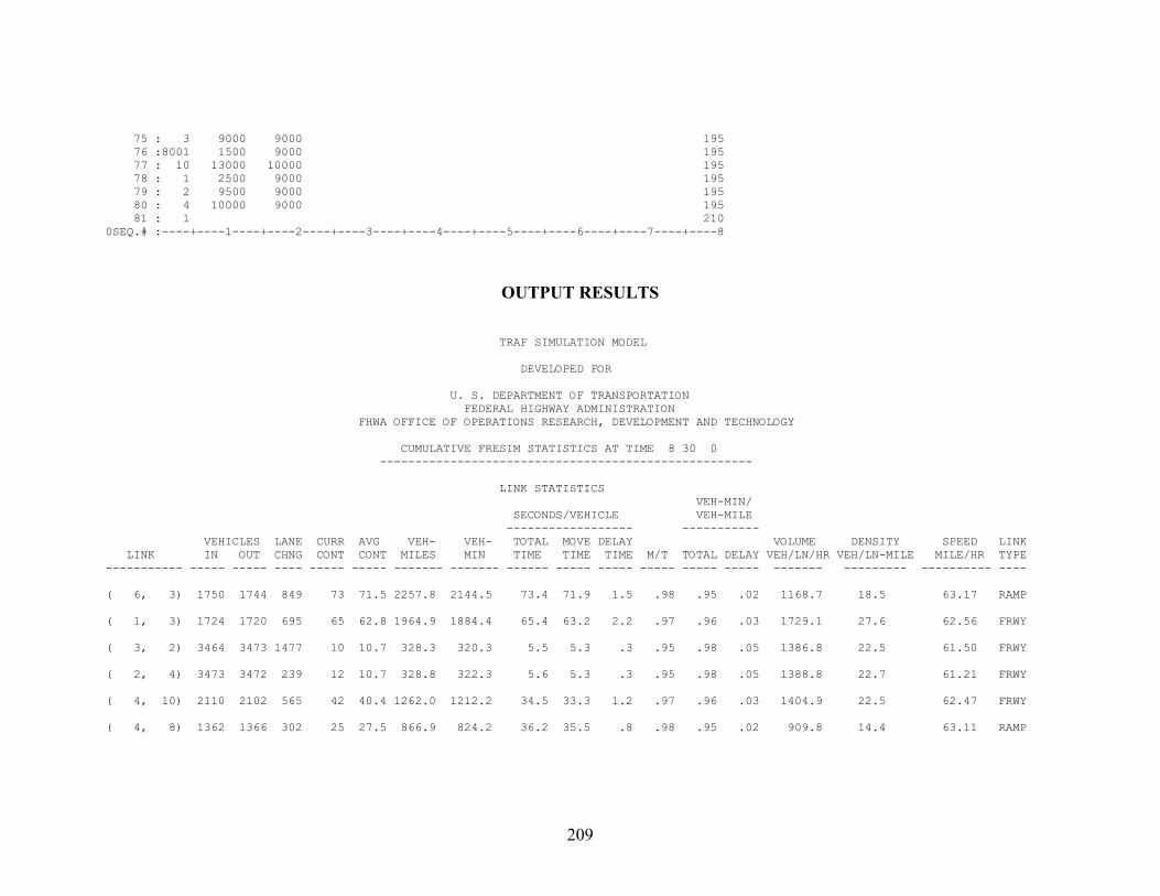
75 : 3 9000 9000 195 76 :8001 1500 9000 195 77 : 10 13000 10000 195 78 : 1 2500 9000 195 79 : 2 9500 9000 195 80 : 4 10000 9000 195 81 : 1 210 0SEQ.# :----+----1----+----2----+----3----+----4----+----5----+----6----+----7----+----8

OUTPUT RESULTS

TRAF SIMULATION MODEL DEVELOPED FOR U. S. DEPARTMENT OF TRANSPORTATION FEDERAL HIGHWAY ADMINISTRATION FHWA OFFICE OF OPERATIONS RESEARCH, DEVELOPMENT AND TECHNOLOGY CUMULATIVE FRESIM STATISTICS AT TIME 8 30 0 ----------------------------------------------------- LINK STATISTICS VEH-MIN/ SECONDS/VEHICLE VEH-MILE ------------------ ----------- VEHICLES LANE CURR AVG VEH- VEH- TOTAL MOVE DELAY VOLUME DENSITY SPEED LINK LINK IN OUT CHNG CONT CONT MILES MIN TIME TIME TIME M/T TOTAL DELAY VEH/LN/HR VEH/LN-MILE MILE/HR TYPE ----------- ----- ----- ---- ----- ----- ------- ------- ------ ----- ----- ----- ----- ----- ------- --------- ---------- ---- ( 6, 3) 1750 1744 849 73 71.5 2257.8 2144.5 73.4 71.9 1.5 .98 .95 .02 1168.7 18.5 63.17 RAMP ( 1, 3) 1724 1720 695 65 62.8 1964.9 1884.4 65.4 63.2 2.2 .97 .96 .03 1729.1 27.6 62.56 FRWY ( 3, 2) 3464 3473 1477 10 10.7 328.3 320.3 5.5 5.3 .3 .95 .98 .05 1386.8 22.5 61.50 FRWY ( 2, 4) 3473 3472 239 12 10.7 328.8 322.3 5.6 5.3 .3 .95 .98 .05 1388.8 22.7 61.21 FRWY ( 4, 10) 2110 2102 565 42 40.4 1262.0 1212.2 34.5 33.3 1.2 .97 .96 .03 1404.9 22.5 62.47 FRWY ( 4, 8) 1362 1366 302 25 27.5 866.9 824.2 36.2 35.5 .8 .98 .95 .02 909.8 14.4 63.11 RAMP

209

APPENDIX D

210

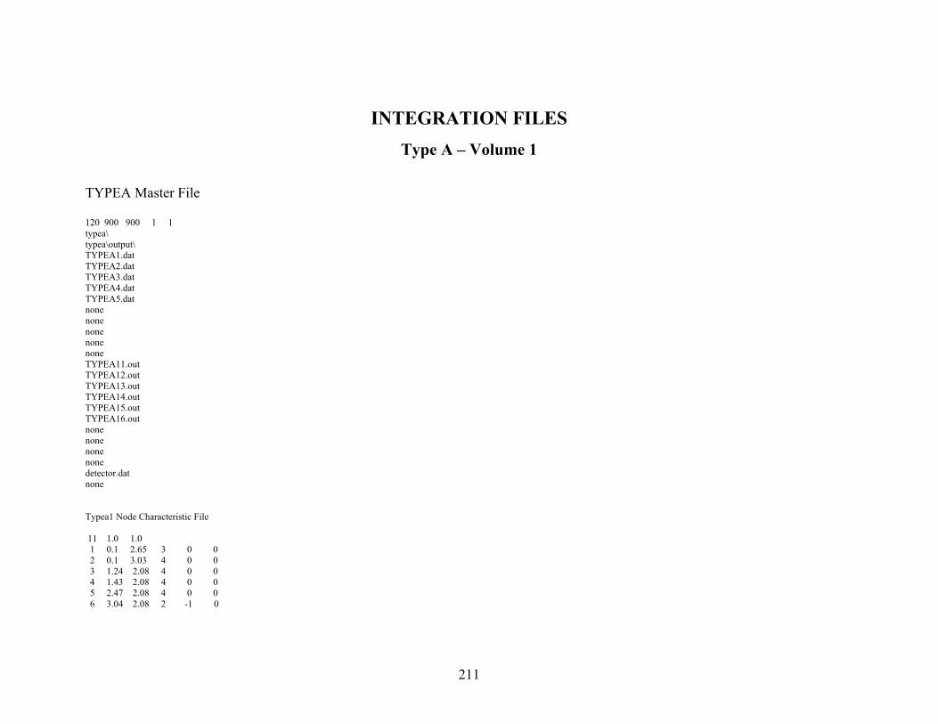
INTEGRATION FILES Type A – Volume 1

TYPEA Master File 120 900 900 1 1 typea\ typea\output\ TYPEA1.dat TYPEA2.dat TYPEA3.dat TYPEA4.dat TYPEA5.dat none none none none none TYPEA11.out TYPEA12.out TYPEA13.out TYPEA14.out TYPEA15.out TYPEA16.out none none none none detector.dat none � Typea1 Node Characteristic File 11 1.0 1.0 1 0.1 2.65 3 0 0 2 0.1 3.03 4 0 0 3 1.24 2.08 4 0 0 4 1.43 2.08 4 0 0 5 2.47 2.08 4 0 0 6 3.04 2.08 2 -1 0

211

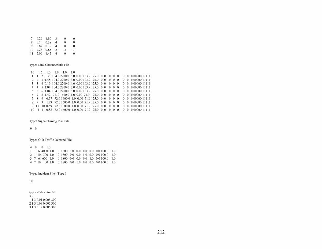
7 0.29 1.80 3 0 0 8 0.1 0.38 4 0 0 9 0.67 0.38 4 0 0 10 2.28 0.85 2 -2 0 11 2.09 1.42 4 0 0 � Typea Link Characteristic File 10 1.6 1.0 1.0 1.0 1.0 1 1 2 0.38 104.0 2200.0 3.0 0.00 103.9 125.0 0 0 0 0 0 0 0 0 00000 11111 2 2 3 1.48 104.0 2200.0 3.0 0.00 103.9 125.0 0 0 0 0 0 0 0 0 00000 11111 3 3 4 0.19 104.0 2200.0 4.0 0.00 103.9 125.0 0 0 0 0 0 0 0 0 00000 11111 4 4 5 1.04 104.0 2200.0 3.0 0.00 103.9 125.0 0 0 0 0 0 0 0 0 00000 11111 5 5 6 1.04 104.0 2200.0 3.0 0.00 103.9 125.0 0 0 0 0 0 0 0 0 00000 11111 6 7 8 1.42 72. 0 1600.0 1.0 0.00 71.9 125.0 0 0 0 0 0 0 0 0 00000 11111 7 8 9 0.57 72.0 1600.0 1.0 0.00 71.9 125.0 0 0 0 0 0 0 0 0 00000 11111 8 9 3 1.79 72.0 1600.0 1.0 0.00 71.9 125.0 0 0 0 0 0 0 0 0 00000 11111 9 11 10 0.59 72.0 1600.0 1.0 0.00 71.9 125.0 0 0 0 0 0 0 0 0 00000 11111 10 4 11 0.88 72.0 1600.0 1.0 0.00 71.9 125.0 0 0 0 0 0 0 0 0 00000 11111 � Typea Signal Timing Plan File 0 0 � Typea O-D Traffic Demand File 4 0 0 1.0 1 1 6 4000 1.0 0 1800 1.0 0.0 0.0 0.0 0.0 100.0 1.0 2 1 10 300 1.0 0 1800 0.0 0.0 1.0 0.0 0.0 100.0 1.0 3 7 6 600 1.0 0 1800 0.0 0.0 0.0 1.0 0.0 100.0 1.0 4 7 10 100 1.0 0 1800 0.0 1.0 0.0 0.0 0.0 100.0 1.0 � Typea Incident File - Type 1 0 � typeav2 detector file 3 0 1 1 3 0.01 0.005 300 2 1 3 0.09 0.005 300 3 1 3 0.19 0.005 300

212

Output File Average Traffic conditions 120 1 1 0.608 6600 3630 3360 0 270 0 0 21.0 21.1 21.1 21.0 21.1 21.0 21.0 0.00 0.00 0.00 0.00 0.00 23.3 20.8 0.0 7.496 14.599 365.648 28.377 67.1 31.0 0.7 1.9 32.7 19.3 2 2.368 6600 480 420 0 60 0 0 82.0 82.2 82.1 82.0 82.9 82.0 82.0 0.00 0.00 0.00 0.00 0.00 48.3 41.6 0.1 14.186 15.023 283.866 51.210 139.1 64.3 1.5 4.0 65.9 41.0

272 1600 30 0 0 0 30 0 113.6 113.7 113.6 113.6 113.6 113.7 113.6 0.00 0.00 0.00 0.00 0.00 12.9 0.4 0.9 2.425 2.133 34.262 4.740 55.6 26.8 0.2 3.2 24.1 16.9

3 0.304 8800 210 180 0 30 0 0 10.5 10.9 10.6 10.5 13.1 10.5 10.5 0.00 0.00 0.00 0.00 0.00 1.1 0.9 0.1 0.359 1.047 21.177 1.295 3.2 1.5 0.0 0.1 1.5 0.9 4 1.664 6600 0 0 0 0 0 0 57.6 57.6 57.6 57.6 57.6 57.6 57.6 0.00 0.00 0.00 0.00 0.00 0.2 0.1 0.0 0.057 0.061 1.109 0.217 0.6 0.3 0.0 0.0 0.3 0.2 5 1.664 6600 0 0 0 0 0 0 57.6 57.6 57.6 57.6 57.6 57.6 57.6 0.00 0.00 0.00 0.00 0.00 0.0 0.0 0.0 0.000 0.000 0.000 0.000 0.0 0.0 0.0 0.0 0.0 0.0 6 2.

7 0.912 1600 0 0 0 0 0 0 45.6 45.6 45.6 45.6 45.6 45.6 45.6 0.00 0.00 0.00 0.00 0.00 0.1 0.0 0.0 0.009 0.008 0.133 0.017 0.2 0.1 0.0 0.0 0.1 0.1 8 2.864 1600 0 0 0 0 0 0 143.2 143.2 143.2 143.2 143.2 143.2 143.2 0.00 0.00 0.00 0.00 0.00 0.0 0.0 0.0 0.000 0.000 0.000 0.000 0.0 0.0 0.0 0.0 0.0 0.0 9 0.944 1600 0 0 0 0 0 0 47.2 47.2 47.2 47.2 47.2 47.2 47.2 0.00 0.00 0.00 0.00 0.00 0.0 0.0 0.0 0.000 0.000 0.000 0.000 0.0 0.0 0.0 0.0 0.0 0.0 10 1.408 1600 0 0 0 0 0 0 70.4 70.4 70.4 70.4 70.4 70.4 70.4 0.00 0.00 0.00 0.00 0.00 0.0 0.0 0.0 0.001 0.001 0.015 0.001 0.0 0.0 0.0 0.0 0.0 0.0

Type A – Volume 2

TYPEAV2 Master File 1800 900 900 1 1 typeav2\ typeav2\output\ TYPEAV21.dat TYPEAV22.dat TYPEAV23.dat TYPEAV24.dat TYPEAV25.dat none none none

213

none none TYPEAV211.out TYPEAV212.out TYPEAV213.out TYPEAV214.out none none none none none none detector.dat none � typea O-D Traffic Demand File 4 0 0 1.0 1 1 6 5000 1.0 0 1800 1.0 0.0 0.0 0.0 0.0 100.0 1.0 2 1 10 450 1.0 0 1800 0.0 0.0 1.0 0.0 0.0 100.0 1.0 3 7 6 800 1.0 0 1800 0.0 0.0 0.0 1.0 0.0 100.0 1.0 4 7 10 100 1.0 0 1800 0.0 1.0 0.0 0.0 0.0 100.0 1.0 � Output File Average Traffic conditions 1800 1 1 0.608 6600 5378 4936 0 442 0 0 21.0 21.2 21.2 21.0 21.2 21.0 21.0 0.00 0.00 0.00 0.00 0.00 32.0 30.7 0.1 161.056 320.430 8225.957 646.615 1381.0 636.6 13.0 40.2 686.3 390.7 2 2.368 6600 5064 4648 0 416 0 0 82.0 86.6 86.4 82.0 89.7 82.0 82.0 0.00 0.00 0.00 0.00 0.00 126.2 122.4 0.4 561.421 1073.019 24062.955 2037.327 5444.4 2517.1 59.6 155.6 2587.5 1602.3 3 0.304 8800 5734 4608 88 414 624 0 10.5 14.3 13.5 14.4 16.8 18.3 10.5 0.00 0.00 0.00 0.00 0.00 23.0 22.9 0.2 169.143 1051.534 23077.895 594.617 991.7 462.8 5.3 41.2 478.7 280.1 4 1.664 6600 5044 4444 0 0 600 0 57.6 57.7 57.7 57.6 57.6 58.1 57.6 0.00 0.00 0.00 0.00 0.00 82.4 80.6 0.0 400.943 722.696 14243.964 1476.557 3556.5 1657.2 29.6 125.1 1726.3 1020.9 5 1.664 6600 4862 4286 0 0 576 0 57.6 57.5 57.5 57.6 57.6 57.5 57.6 0.00 0.00 0.00 0.00 0.00 79.1 77.3 0.0 350.127 340.359 6139.452 1271.369 3414.7 1579.7 37.2 97.4 1625.0 1003.5 6 2.272 1600 832 0 94 0 738 0 113.6 113.7 113.6 113.7 113.6 113.8 113.6 0.00 0.00 0.00 0.00 0.00 27.4 1.1 0.1 76.862 67.662 1084.634 148.736 1768.3 853.9 7.7 104.6 755.2 543.2 7 0.912 1600 812 0 90 0 722 0 45.6 45.5 45.6 45.5 45.6 45.5 45.6 0.00 0.00 0.00 0.00 0.00 10.4 0.5 0.0 28.881 25.503 405.708 54.010 671.4 323.0 2.9 38.4 294.8 202.7

214

8 2.864 1600 722 0 88 0 634 0 143.2 143.4 143.2 143.5 143.2 143.4 143.2 0.00 0.00 0.00 0.00 0.00 30.9 0.7 0.1 85.228 75.558 1197.940 158.633 1995.4 960.2 8.7 114.0 877.6 602.2 9 0.944 1600 464 0 84 380 0 0 47.2 47.0 47.2 47.0 47.0 47.2 47.2 0.00 0.00 0.00 0.00 0.00 6.2 0.3 0.0 17.337 15.314 243.306 32.370 403.7 194.1 1.8 23.0 177.5 121.8 10 1.408 1600 486 0 86 400 0 0 70.4 70.5 70.4 70.6 70.5 70.4 70.4 0.00 0.00 0.00 0.00 0.00 9.7 0.5 0.1 27.866 29.741 543.681 56.667 625.9 301.5 2.7 36.3 269.8 191.0

Type A – Volume 3 TYPEAV3 Master File 1800 900 900 1 1 typeav3\ typeav3\output\ TYPEAV31.dat TYPEAV32.dat TYPEAV33.dat TYPEAV34.dat TYPEAV35.dat none none none none none TYPEAV311.out TYPEAV312.out TYPEAV313.out TYPEAV314.out none none none none none none detector.dat none �

215

typea O-D Traffic Demand File 4 0 0 1.0 1 1 6 6000 1.0 0 1800 1.0 0.0 0.0 0.0 0.0 100.0 1.0 2 1 10 600 1.0 0 1800 0.0 0.0 1.0 0.0 0.0 100.0 1.0 3 7 6 1000 1.0 0 1800 0.0 0.0 0.0 1.0 0.0 100.0 1.0 4 7 10 100 1.0 0 1800 0.0 1.0 0.0 0.0 0.0 100.0 1.0 Output File Average Traffic conditions 1800 1 1 0.608 6600 5732 5204 0 528 0 0 21.0 35.6 35.6 21.0 35.2 21.0 21.0 0.00 0.00 0.00 0.00 0.00 57.8 57.7 0.4 134.169 155.336 2560.181 262.724 2494.7 1152.2 19.5 78.9 1275.9 686.0 2 2.368 6600 5170 4680 0 490 0 0 82.0 151.5 150.7 82.0 159.7 82.0 82.0 0.00 0.00 0.00 0.00 0.00 232.8 232.8 1.0 716.385 1692.751 38533.410 1964.148 10074.4 4751.0 34.2 497.8 4400.5 3025.8 3 0.304 8800 6030 4640 90 490 810 0 10.5 15.7 14.7 16.4 18.4 20.3 10.5 0.00 0.00 0.00 0.00 0.00 26.6 26.5 0.2 238.804 1606.733 35272.684 855.954 1146.3 516.9 3.0 36.7 660.9 265.1 4 1.664 6600 5264 4490 0 0 774 0 57.6 57.7 57.7 57.6 57.6 57.8 57.6 0.00 0.00 0.00 0.00 0.00 85.9 84.7 0.0 409.945 640.371 12753.462 1527.088 3705.7 1718.6 32.6 119.1 1825.9 1054.3 5 1.664 6600 5080 4336 0 0 744 0 57.6 57.5 57.5 57.6 57.6 57.5 57.6 0.00 0.00 0.00 0.00 0.00 82.7 81.7 0.0 366.567 356.702 6431.008 1333.099 3570.6 1651.9 38.7 101.7 1703.2 1047.7 6 2.272 1600 1034 0 98 0 936 0 113.6 113.8 113.6 113.8 113.6 113.9 113.6 0.00 0.00 0.00 0.00 0.00 33.8 1.7 0.1 95.342 83.796 1347.680 186.276 2183.8 1056.1 9.5 131.2 919.8 676.2 7 0.912 1600 1018 0 94 0 924 0 45.6 45.5 45.6 45.5 45.6 45.5 45.6 0.00 0.00 0.00 0.00 0.00 13.0 0.6 0.0 36.153 31.928 508.459 67.645 839.6 404.0 3.7 48.1 368.3 253.6 8 2.864 1600 912 0 90 0 822 0 143.2 148.1 143.2 147.6 143.2 148.1 143.2 0.00 0.00 0.00 0.00 0.00 39.9 3.2 0.4 106.818 95.561 1498.392 195.934 2577.8 1240.3 11.2 147.4 1132.2 778.3 9 0.944 1600 532 0 80 452 0 0 47.2 47.0 47.2 47.0 47.0 47.2 47.2 0.00 0.00 0.00 0.00 0.00 7.2 0.3 0.0 19.863 17.548 278.875 37.083 462.5 222.4 2.0 26.4 203.3 139.5 10 1.408 1600 558 0 86 472 0 0 70.4 70.5 70.4 70.7 70.5 70.4 70.4 0.00 0.00 0.00 0.00 0.00 11.1 0.6 0.1 31.983 33.148 595.084 65.037 720.0 347.1 3.1 42.1 308.9 220.4

Type A – Volume 4 TYPEAV4 Master File 1800 900 900 1 1 typeav4\ typeav4\output\

216

TYPEAV41.dat TYPEAV42.dat TYPEAV43.dat TYPEAV44.dat TYPEAV45.dat none none none none none TYPEAV411.out TYPEAV412.out TYPEAV413.out TYPEAV414.out none none none none none none detector.dat none � typeav4 O-D Traffic Demand File 4 0 0 1.0 1 1 6 6000 1.0 0 1800 1.0 0.0 0.0 0.0 0.0 100.0 1.0 2 1 10 800 1.0 0 1800 0.0 0.0 1.0 0.0 0.0 100.0 1.0 3 7 6 1200 1.0 0 1800 0.0 0.0 0.0 1.0 0.0 100.0 1.0 4 7 10 300 1.0 0 1800 0.0 1.0 0.0 0.0 0.0 100.0 1.0 � Output File Average Traffic conditions 1800 1 1 0.608 6600 5658 4990 0 668 0 0 21.0 37.3 37.4 21.0 36.4 21.0 21.0 0.00 0.00 0.00 0.00 0.00 59.7 59.7 0.5 132.196 151.730 2455.347 238.604 2580.1 1192.3 19.8 82.7 1321.1 708.6 2 2.368 6600 5126 4518 0 608 0 0 82.0 156.4 155.4 82.0 164.2 82.0 82.0 0.00 0.00 0.00 0.00 0.00 236.2 236.1 1.1 751.025 2064.852 47104.160 2083.406 10218.3 4824.4 31.3 510.9 4354.1 3117.6 3 0.304 8800 6162 4482 234 602 844 0 10.5 15.8 14.4 18.1 19.5 20.1 10.5 0.00 0.00 0.00 0.00 0.00 27.3 27.3 0.2 248.863 1682.238 37167.281 882.347 1179.0 527.1 2.5 34.0 696.5 264.6

217

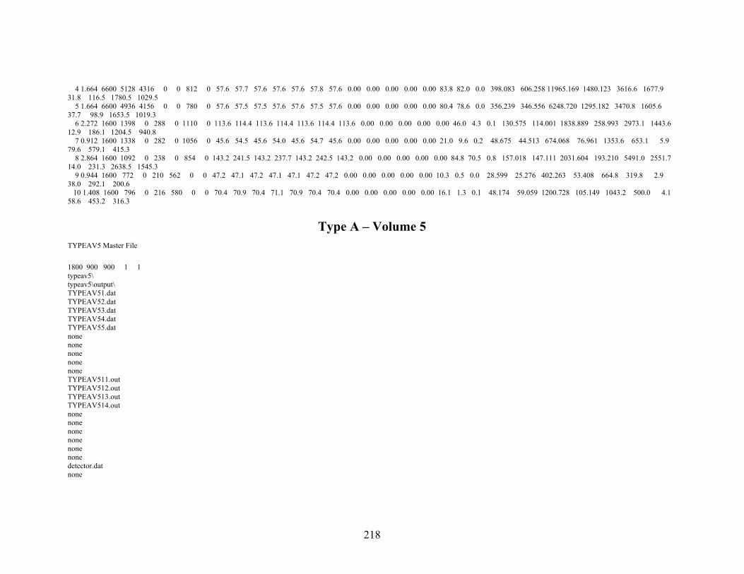
4 1.664 6600 5128 4316 0 0 812 0 57.6 57.7 57.6 57.6 57.6 57.8 57.6 0.00 0.00 0.00 0.00 0.00 83.8 82.0 0.0 398.083 606.258 11965.169 1480.123 3616.6 1677.9 31.8 116.5 1780.5 1029.5 5 1.664 6600 4936 4156 0 0 780 0 57.6 57.5 57.5 57.6 57.6 57.5 57.6 0.00 0.00 0.00 0.00 0.00 80.4 78.6 0.0 356.239 346.556 6248.720 1295.182 3470.8 1605.6 37.7 98.9 1653.5 1019.3 6 2.272 1600 1398 0 288 0 1110 0 113.6 114.4 113.6 114.4 113.6 114.4 113.6 0.00 0.00 0.00 0.00 0.00 46.0 4.3 0.1 130.575 114.001 1838.889 258.993 2973.1 1443.6 12.9 186.1 1204.5 940.8 7 0.912 1600 1338 0 282 0 1056 0 45.6 54.5 45.6 54.0 45.6 54.7 45.6 0.00 0.00 0.00 0.00 0.00 21.0 9.6 0.2 48.675 44.513 674.068 76.961 1353.6 653.1 5.9 79.6 579.1 415.3 8 2.864 1600 1092 0 238 0 854 0 143.2 241.5 143.2 237.7 143.2 242.5 143.2 0.00 0.00 0.00 0.00 0.00 84.8 70.5 0.8 157.018 147.111 2031.604 193.210 5491.0 2551.7 14.0 231.3 2638.5 1545.3 9 0.944 1600 772 0 210 562 0 0 47.2 47.1 47.2 47.1 47.1 47.2 47.2 0.00 0.00 0.00 0.00 0.00 10.3 0.5 0.0 28.599 25.276 402.263 53.408 664.8 319.8 2.9 38.0 292.1 200.6 10 1.408 1600 796 0 216 580 0 0 70.4 70.9 70.4 71.1 70.9 70.4 70.4 0.00 0.00 0.00 0.00 0.00 16.1 1.3 0.1 48.174 59.059 1200.728 105.149 1043.2 500.0 4.1 58.6 453.2 316.3

Type A – Volume 5 TYPEAV5 Master File 1800 900 900 1 1 typeav5\ typeav5\output\ TYPEAV51.dat TYPEAV52.dat TYPEAV53.dat TYPEAV54.dat TYPEAV55.dat none none none none none TYPEAV511.out TYPEAV512.out TYPEAV513.out TYPEAV514.out none none none none none none detector.dat none �

218

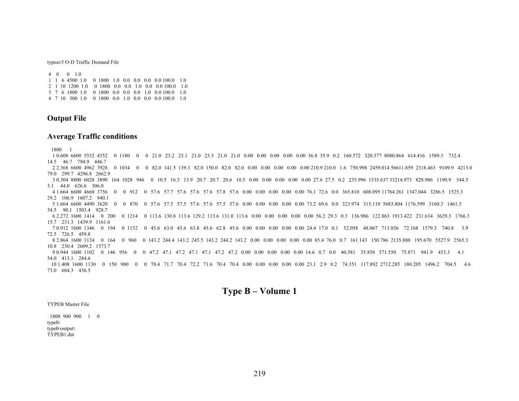
typeav5 O-D Traffic Demand File 4 0 0 1.0 1 1 6 4500 1.0 0 1800 1.0 0.0 0.0 0.0 0.0 100.0 1.0 2 1 10 1200 1.0 0 1800 0.0 0.0 1.0 0.0 0.0 100.0 1.0 3 7 6 1800 1.0 0 1800 0.0 0.0 0.0 1.0 0.0 100.0 1.0 4 7 10 300 1.0 0 1800 0.0 1.0 0.0 0.0 0.0 100.0 1.0 � Output File Average Traffic conditions 1800 1 1 0.608 6600 5532 4352 0 1180 0 0 21.0 23.2 23.1 21.0 23.3 21.0 21.0 0.00 0.00 0.00 0.00 0.00 36.8 35.9 0.2 160.572 320.377 8080.864 614.416 1589.3 732.4 14.5 46.7 794.9 446.7 2 2.368 6600 4962 3928 0 1034 0 0 82.0 141.5 139.3 82.0 150.0 82.0 82.0 0.00 0.00 0.00 0.00 0.00 210.9 210.0 1.6 750.998 2459.014 56611.859 2318.463 9109.9 4213.0 79.0 299.7 4296.8 2662.9 3 0.304 8800 6028 3890 164 1028 946 0 10.5 16.3 13.9 20.7 20.7 20.6 10.5 0.00 0.00 0.00 0.00 0.00 27.6 27.5 0.2 235.996 1535.637 33214.973 828.986 1190.9 544.5 3.1 44.0 626.6 306.0 4 1.664 6600 4668 3756 0 0 912 0 57.6 57.7 57.6 57.6 57.6 57.8 57.6 0.00 0.00 0.00 0.00 0.00 76.1 72.6 0.0 365.810 608.095 11764.261 1347.044 3286.5 1525.3 29.2 106.9 1607.2 940.1 5 1.664 6600 4490 3620 0 0 870 0 57.6 57.5 57.5 57.6 57.6 57.5 57.6 0.00 0.00 0.00 0.00 0.00 73.2 69.6 0.0 323.974 315.110 5683.804 1176.599 3160.3 1461.5 34.5 90.1 1503.4 928.7 6 2.272 1600 1414 0 200 0 1214 0 113.6 130.8 113.6 129.2 113.6 131.0 113.6 0.00 0.00 0.00 0.00 0.00 56.2 29.3 0.3 136.986 122.863 1913.422 231.634 3629.3 1766.3 15.7 231.3 1439.9 1161.6 7 0.912 1600 1346 0 194 0 1152 0 45.6 63.0 45.6 63.8 45.6 62.8 45.6 0.00 0.00 0.00 0.00 0.00 24.4 17.0 0.1 52.058 48.067 713.856 72.168 1579.3 740.8 3.9 72.5 726.5 459.8 8 2.864 1600 1124 0 164 0 960 0 143.2 244.4 143.2 245.5 143.2 244.2 143.2 0.00 0.00 0.00 0.00 0.00 85.4 76.0 0.7 161.143 150.786 2135.880 195.670 5527.9 2565.3 10.8 230.4 2609.2 1573.7 9 0.944 1600 1102 0 146 956 0 0 47.2 47.1 47.2 47.1 47.1 47.2 47.2 0.00 0.00 0.00 0.00 0.00 14.6 0.7 0.0 40.581 35.858 571.550 75.871 941.9 453.3 4.1 54.0 413.1 284.6 10 1.408 1600 1130 0 150 980 0 0 70.4 71.7 70.4 72.2 71.6 70.4 70.4 0.00 0.00 0.00 0.00 0.00 23.1 2.9 0.2 74.351 117.892 2712.285 180.205 1496.2 704.5 4.6 73.0 684.3 436.5

Type B – Volume 1 TYPEB Master File 1800 900 900 1 0 typeb\ typeb\output\ TYPEB1.dat

219

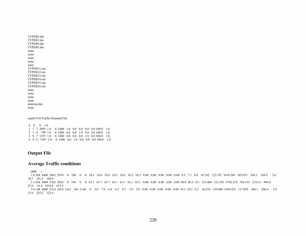
TYPEB2.dat TYPEB3.dat TYPEB4.dat TYPEB5.dat none none none none none TYPEB11.out TYPEB12.out TYPEB13.out TYPEB14.out TYPEB15.out TYPEB16.out none none none none detector.dat none � typeb O-D Traffic Demand File 4 0 0 1.0 1 1 7 2095 1.0 0 1800 1.0 0.0 0.0 0.0 0.0 100.0 1.0 2 1 11 799 1.0 0 1800 0.0 0.0 1.0 0.0 0.0 100.0 1.0 3 9 7 1197 1.0 0 1800 0.0 0.0 0.0 1.0 0.0 100.0 1.0 4 9 11 1497 1.0 0 1800 0.0 1.0 0.0 0.0 0.0 100.0 1.0 � Output File Average Traffic conditions 1800 1 1 0.304 4400 2862 2074 0 788 0 0 10.5 10.6 10.6 10.5 10.6 10.5 10.5 0.00 0.00 0.00 0.00 0.00 8.5 7.1 0.0 45.762 125.187 3419.396 185.933 368.1 169.9 3.6 10.7 181.5 104.9 2 1.824 4400 2762 2016 0 746 0 0 63.1 63.7 63.7 63.1 63.7 63.1 63.1 0.00 0.00 0.00 0.00 0.00 49.8 40.2 0.1 213.484 212.391 3792.219 764.153 2152.4 994.0 23.6 61.4 1018.8 633.5 3 0.144 8800 5314 2014 1412 744 1144 0 5.0 7.0 6.9 6.5 8.1 7.0 5.0 0.00 0.00 0.00 0.00 0.00 10.3 10.2 0.2 36.254 139.040 3428.452 117.859 446.1 206.4 3.0 15.6 225.2 122.6

220

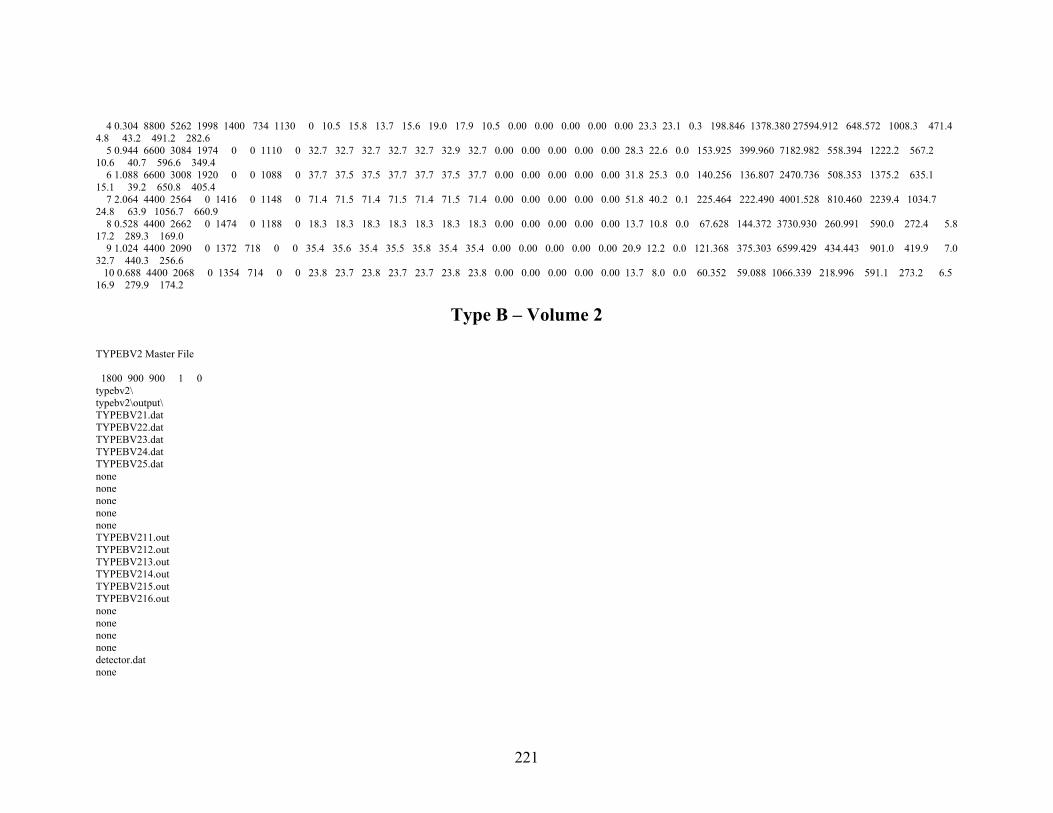
4 0.304 8800 5262 1998 1400 734 1130 0 10.5 15.8 13.7 15.6 19.0 17.9 10.5 0.00 0.00 0.00 0.00 0.00 23.3 23.1 0.3 198.846 1378.380 27594.912 648.572 1008.3 471.4 4.8 43.2 491.2 282.6 5 0.944 6600 3084 1974 0 0 1110 0 32.7 32.7 32.7 32.7 32.7 32.9 32.7 0.00 0.00 0.00 0.00 0.00 28.3 22.6 0.0 153.925 399.960 7182.982 558.394 1222.2 567.2 10.6 40.7 596.6 349.4 6 1.088 6600 3008 1920 0 0 1088 0 37.7 37.5 37.5 37.7 37.7 37.5 37.7 0.00 0.00 0.00 0.00 0.00 31.8 25.3 0.0 140.256 136.807 2470.736 508.353 1375.2 635.1 15.1 39.2 650.8 405.4 7 2.064 4400 2564 0 1416 0 1148 0 71.4 71.5 71.4 71.5 71.4 71.5 71.4 0.00 0.00 0.00 0.00 0.00 51.8 40.2 0.1 225.464 222.490 4001.528 810.460 2239.4 1034.7 24.8 63.9 1056.7 660.9 8 0.528 4400 2662 0 1474 0 1188 0 18.3 18.3 18.3 18.3 18.3 18.3 18.3 0.00 0.00 0.00 0.00 0.00 13.7 10.8 0.0 67.628 144.372 3730.930 260.991 590.0 272.4 5.8 17.2 289.3 169.0 9 1.024 4400 2090 0 1372 718 0 0 35.4 35.6 35.4 35.5 35.8 35.4 35.4 0.00 0.00 0.00 0.00 0.00 20.9 12.2 0.0 121.368 375.303 6599.429 434.443 901.0 419.9 7.0 32.7 440.3 256.6 10 0.688 4400 2068 0 1354 714 0 0 23.8 23.7 23.8 23.7 23.7 23.8 23.8 0.00 0.00 0.00 0.00 0.00 13.7 8.0 0.0 60.352 59.088 1066.339 218.996 591.1 273.2 6.5 16.9 279.9 174.2

Type B – Volume 2 TYPEBV2 Master File 1800 900 900 1 0 typebv2\ typebv2\output\ TYPEBV21.dat TYPEBV22.dat TYPEBV23.dat TYPEBV24.dat TYPEBV25.dat none none none none none TYPEBV211.out TYPEBV212.out TYPEBV213.out TYPEBV214.out TYPEBV215.out TYPEBV216.out none none none none detector.dat none �

221

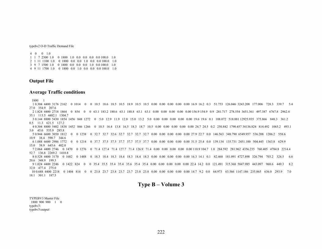
typebv2 O-D Traffic Demand File 4 0 0 1.0 1 1 7 2300 1.0 0 1800 1.0 0.0 0.0 0.0 0.0 100.0 1.0 2 1 11 1100 1.0 0 1800 0.0 0.0 1.0 0.0 0.0 100.0 1.0 3 9 7 1500 1.0 0 1800 0.0 0.0 0.0 1.0 0.0 100.0 1.0 4 9 11 1700 1.0 0 1800 0.0 1.0 0.0 0.0 0.0 100.0 1.0 �

Output File Average Traffic conditions 1800 1 1 0.304 4400 3176 2162 0 1014 0 0 10.5 18.6 18.5 10.5 18.9 10.5 10.5 0.00 0.00 0.00 0.00 0.00 16.9 16.2 0.3 51.753 126.046 3243.208 177.006 728.3 339.7 5.4 27.0 354.9 207.6 2 1.824 4400 2718 1864 0 854 0 0 63.1 183.2 180.6 63.1 188.8 63.1 63.1 0.00 0.00 0.00 0.00 0.00 156.9 154.9 0.9 281.717 278.554 3651.361 497.387 6767.8 2962.4 35.1 113.5 4482.1 1304.7 3 0.144 8800 5430 1854 1456 848 1272 0 5.0 12.9 11.9 12.8 15.0 13.2 5.0 0.00 0.00 0.00 0.00 0.00 19.6 19.6 0.1 108.072 518.881 12925.935 375.866 848.3 361.2 0.5 11.3 621.5 127.2 4 0.304 8800 5402 1838 1452 846 1266 0 10.5 16.4 13.8 16.5 18.3 18.7 10.5 0.00 0.00 0.00 0.00 0.00 24.7 24.5 0.2 250.842 1790.457 34136.824 814.492 1065.2 493.1 3.0 45.0 535.9 285.8 5 0.944 6600 3050 1812 0 0 1238 0 32.7 32.7 32.6 32.7 32.7 32.7 32.7 0.00 0.00 0.00 0.00 0.00 27.9 22.7 0.0 146.563 348.790 6549.957 536.208 1206.2 558.6 10.9 38.4 590.7 344.6 6 1.088 6600 2986 1772 0 0 1214 0 37.7 37.5 37.5 37.7 37.7 37.5 37.7 0.00 0.00 0.00 0.00 0.00 31.5 25.4 0.0 139.134 135.731 2451.100 504.445 1363.8 629.9 15.0 38.9 645.6 402.0 7 2.064 4400 2746 0 1470 0 1276 0 71.4 127.4 71.4 127.7 71.4 126.9 71.4 0.00 0.00 0.00 0.00 0.00 110.9 104.7 1.0 284.592 281.962 4356.235 760.405 4784.8 2214.4 52.7 136.8 2269.2 1410.8 8 0.528 4400 3170 0 1682 0 1488 0 18.3 18.4 18.3 18.4 18.3 18.4 18.3 0.00 0.00 0.00 0.00 0.00 16.3 14.1 0.1 82.468 181.091 4727.898 326.794 703.2 324.5 6.6 20.6 348.9 199.3 9 1.024 4400 2246 0 1422 824 0 0 35.4 35.5 35.4 35.4 35.6 35.4 35.4 0.00 0.00 0.00 0.00 0.00 22.4 14.2 0.0 121.491 315.368 5847.985 443.097 968.6 449.3 8.2 32.0 477.4 275.0 10 0.688 4400 2218 0 1404 814 0 0 23.8 23.7 23.8 23.7 23.7 23.8 23.8 0.00 0.00 0.00 0.00 0.00 14.7 9.2 0.0 64.973 63.566 1147.186 235.865 636.0 293.9 7.0 18.1 301.1 187.5

Type B – Volume 3 TYPEBV3 Master File 1800 900 900 1 0 typebv3\ typebv3\output\

222

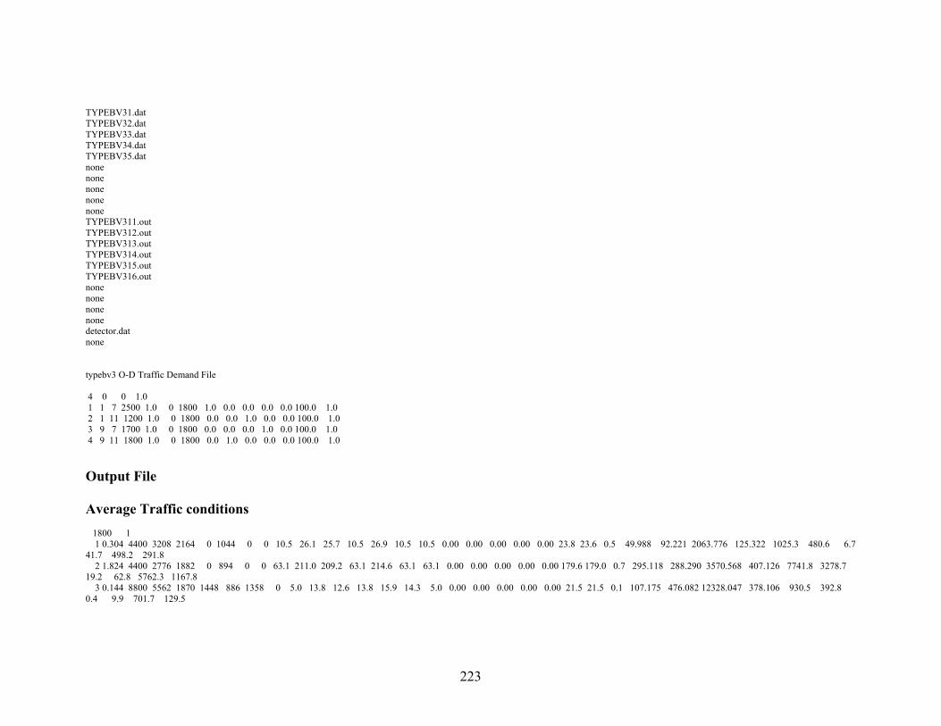
TYPEBV31.dat TYPEBV32.dat TYPEBV33.dat TYPEBV34.dat TYPEBV35.dat none none none none none TYPEBV311.out TYPEBV312.out TYPEBV313.out TYPEBV314.out TYPEBV315.out TYPEBV316.out none none none none detector.dat none � typebv3 O-D Traffic Demand File 4 0 0 1.0 1 1 7 2500 1.0 0 1800 1.0 0.0 0.0 0.0 0.0 100.0 1.0 2 1 11 1200 1.0 0 1800 0.0 0.0 1.0 0.0 0.0 100.0 1.0 3 9 7 1700 1.0 0 1800 0.0 0.0 0.0 1.0 0.0 100.0 1.0 4 9 11 1800 1.0 0 1800 0.0 1.0 0.0 0.0 0.0 100.0 1.0 �

Output File Average Traffic conditions 1800 1 1 0.304 4400 3208 2164 0 1044 0 0 10.5 26.1 25.7 10.5 26.9 10.5 10.5 0.00 0.00 0.00 0.00 0.00 23.8 23.6 0.5 49.988 92.221 2063.776 125.322 1025.3 480.6 6.7 41.7 498.2 291.8 2 1.824 4400 2776 1882 0 894 0 0 63.1 211.0 209.2 63.1 214.6 63.1 63.1 0.00 0.00 0.00 0.00 0.00 179.6 179.0 0.7 295.118 288.290 3570.568 407.126 7741.8 3278.7 19.2 62.8 5762.3 1167.8 3 0.144 8800 5562 1870 1448 886 1358 0 5.0 13.8 12.6 13.8 15.9 14.3 5.0 0.00 0.00 0.00 0.00 0.00 21.5 21.5 0.1 107.175 476.082 12328.047 378.106 930.5 392.8 0.4 9.9 701.7 129.5

223

4 0.304 8800 5512 1860 1434 870 1348 0 10.5 16.4 13.7 16.7 18.3 18.6 10.5 0.00 0.00 0.00 0.00 0.00 25.3 25.2 0.2 262.507 1901.766 36734.961 856.968 1091.7 508.2 3.0 48.8 527.3 303.2 5 0.944 6600 3152 1828 0 0 1324 0 32.7 32.7 32.6 32.7 32.7 32.7 32.7 0.00 0.00 0.00 0.00 0.00 28.9 23.3 0.0 151.190 352.952 6578.758 552.651 1250.4 579.0 11.4 39.7 611.4 357.6 6 1.088 6600 3090 1788 0 0 1302 0 37.7 37.5 37.5 37.7 37.7 37.5 37.7 0.00 0.00 0.00 0.00 0.00 32.6 26.2 0.0 143.672 140.114 2530.057 520.739 1408.5 650.5 15.5 40.2 666.5 415.2 7 2.064 4400 2832 0 1462 0 1370 0 71.4 190.0 71.4 190.2 71.4 189.9 71.4 0.00 0.00 0.00 0.00 0.00 167.9 165.4 0.9 318.187 311.150 4216.849 565.871 7238.3 3181.1 36.6 129.1 4452.6 1590.9 8 0.528 4400 3296 0 1698 0 1598 0 18.3 29.4 18.3 29.6 18.3 29.1 18.3 0.00 0.00 0.00 0.00 0.00 28.0 26.7 0.3 86.121 174.211 4266.500 278.238 1209.6 561.9 9.6 41.9 597.6 341.7 9 1.024 4400 2248 0 1394 854 0 0 35.4 35.5 35.4 35.5 35.6 35.4 35.4 0.00 0.00 0.00 0.00 0.00 22.5 14.4 0.0 123.754 333.645 6206.657 451.897 971.8 451.1 8.2 32.6 478.0 276.2 10 0.688 4400 2212 0 1376 836 0 0 23.8 23.7 23.8 23.7 23.7 23.8 23.8 0.00 0.00 0.00 0.00 0.00 14.7 9.2 0.0 64.938 63.671 1149.036 236.040 635.3 293.6 7.0 18.1 301.2 187.1

Type B – Volume 4 TYPEBV4 Master File 1800 900 900 1 0 typebv4\ typebv4\output\ TYPEBV41.dat TYPEBv42.dat TYPEBv43.dat TYPEBv44.dat TYPEBv45.dat none none none none none TYPEBv411.out TYPEBv412.out TYPEBv413.out TYPEBv414.out TYPEBv415.out TYPEBv416.out none none none none detector.dat none �

224

typebv4 O-D Traffic Demand File 4 0 0 1.0 1 1 7 3000 1.0 0 1800 1.0 0.0 0.0 0.0 0.0 100.0 1.0 2 1 11 1500 1.0 0 1800 0.0 0.0 1.0 0.0 0.0 100.0 1.0 3 9 7 2000 1.0 0 1800 0.0 0.0 0.0 1.0 0.0 100.0 1.0 4 9 11 2000 1.0 0 1800 0.0 1.0 0.0 0.0 0.0 100.0 1.0 �

Output File Average Traffic conditions 1800 1 1 0.304 4400 3178 2138 0 1040 0 0 10.5 30.1 29.9 10.5 30.5 10.5 10.5 0.00 0.00 0.00 0.00 0.00 27.0 27.0 0.6 46.632 61.388 1014.178 89.433 1165.9 547.1 7.3 48.6 565.2 331.8 2 1.824 4400 2736 1846 0 890 0 0 63.1 227.1 226.1 63.1 229.3 63.1 63.1 0.00 0.00 0.00 0.00 0.00 190.8 189.6 0.6 293.984 285.903 3344.378 338.254 8228.1 3452.3 8.0 59.7 6501.9 1024.2 3 0.144 8800 5522 1828 1404 884 1406 0 5.0 13.9 13.1 13.5 15.7 14.2 5.0 0.00 0.00 0.00 0.00 0.00 21.5 21.5 0.1 113.410 525.827 13669.019 402.206 928.3 391.1 0.3 9.3 705.9 125.9 4 0.304 8800 5484 1818 1394 880 1392 0 10.5 16.2 13.7 16.1 18.0 18.4 10.5 0.00 0.00 0.00 0.00 0.00 24.8 24.7 0.2 260.860 1878.227 35750.379 844.580 1069.5 498.8 2.9 48.5 510.7 300.0 5 0.944 6600 3154 1788 0 0 1366 0 32.7 32.7 32.6 32.7 32.7 32.8 32.7 0.00 0.00 0.00 0.00 0.00 28.9 23.6 0.0 153.062 371.160 6752.865 555.942 1250.3 579.7 11.3 40.6 608.0 358.9 6 1.088 6600 3076 1750 0 0 1326 0 37.7 37.5 37.5 37.7 37.7 37.5 37.7 0.00 0.00 0.00 0.00 0.00 32.6 26.4 0.0 143.605 140.000 2528.235 520.327 1408.2 650.4 15.5 40.1 666.3 415.2 7 2.064 4400 2828 0 1408 0 1420 0 71.4 219.0 71.4 220.4 71.4 217.6 71.4 0.00 0.00 0.00 0.00 0.00 191.1 190.3 0.7 326.631 317.788 4033.686 457.883 8237.4 3503.5 21.4 73.3 5700.2 1481.9 8 0.528 4400 3308 0 1672 0 1636 0 18.3 42.8 18.3 43.2 18.3 42.5 18.3 0.00 0.00 0.00 0.00 0.00 40.4 40.0 0.5 87.201 130.589 2660.843 211.966 1744.9 814.2 11.7 67.2 862.9 489.7 9 1.024 4400 2232 0 1376 856 0 0 35.4 35.5 35.4 35.5 35.6 35.4 35.4 0.00 0.00 0.00 0.00 0.00 22.3 13.7 0.0 122.623 332.103 6051.813 445.087 960.9 446.2 8.0 32.5 473.3 272.7 10 0.688 4400 2200 0 1350 850 0 0 23.8 23.7 23.8 23.7 23.7 23.8 23.8 0.00 0.00 0.00 0.00 0.00 14.6 9.0 0.0 64.487 63.163 1139.916 234.172 631.3 291.7 6.9 18.0 299.1 186.0

Type B – Volume 5

225

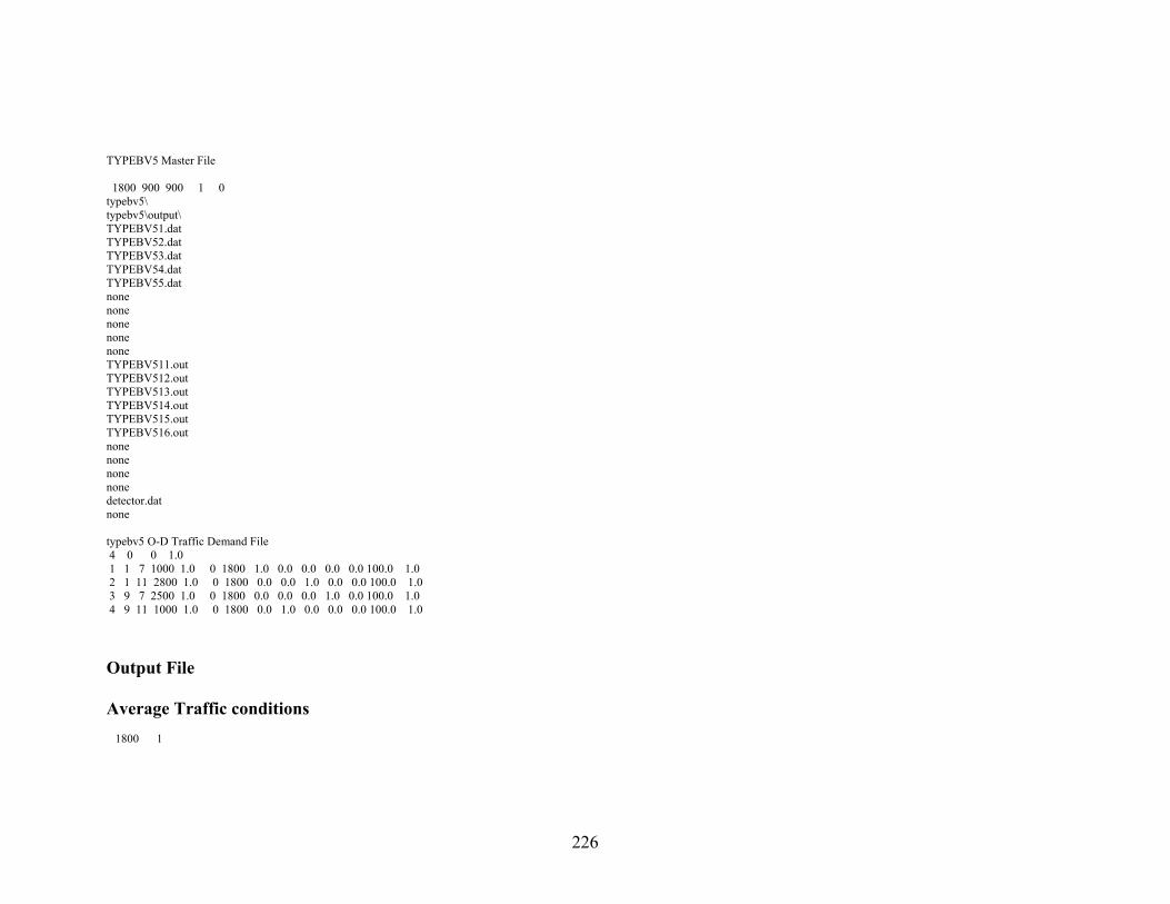
TYPEBV5 Master File 1800 900 900 1 0 typebv5\ typebv5\output\ TYPEBV51.dat TYPEBV52.dat TYPEBV53.dat TYPEBV54.dat TYPEBV55.dat none none none none none TYPEBV511.out TYPEBV512.out TYPEBV513.out TYPEBV514.out TYPEBV515.out TYPEBV516.out none none none none detector.dat none typebv5 O-D Traffic Demand File 4 0 0 1.0 1 1 7 1000 1.0 0 1800 1.0 0.0 0.0 0.0 0.0 100.0 1.0 2 1 11 2800 1.0 0 1800 0.0 0.0 1.0 0.0 0.0 100.0 1.0 3 9 7 2500 1.0 0 1800 0.0 0.0 0.0 1.0 0.0 100.0 1.0 4 9 11 1000 1.0 0 1800 0.0 1.0 0.0 0.0 0.0 100.0 1.0 � Output File Average Traffic conditions 1800 1

226

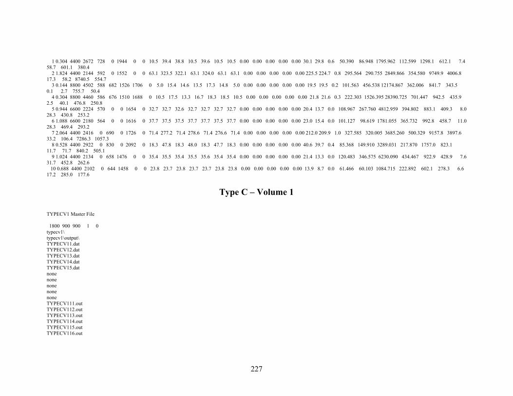
1 0.304 4400 2672 728 0 1944 0 0 10.5 39.4 38.8 10.5 39.6 10.5 10.5 0.00 0.00 0.00 0.00 0.00 30.1 29.8 0.6 50.390 86.948 1795.962 112.599 1298.1 612.1 7.4 58.7 601.1 380.4 2 1.824 4400 2144 592 0 1552 0 0 63.1 323.5 322.1 63.1 324.0 63.1 63.1 0.00 0.00 0.00 0.00 0.00 225.5 224.7 0.8 295.564 290.755 2849.866 354.580 9749.9 4006.8 17.3 58.2 8740.5 554.7 3 0.144 8800 4502 588 682 1526 1706 0 5.0 15.4 14.6 13.5 17.3 14.8 5.0 0.00 0.00 0.00 0.00 0.00 19.5 19.5 0.2 101.563 456.538 12174.867 362.006 841.7 343.5 0.1 2.7 755.7 50.4 4 0.304 8800 4460 586 676 1510 1688 0 10.5 17.5 13.3 16.7 18.3 18.5 10.5 0.00 0.00 0.00 0.00 0.00 21.8 21.6 0.3 222.303 1526.395 28390.725 701.447 942.5 435.9 2.5 40.1 476.8 250.8 5 0.944 6600 2224 570 0 0 1654 0 32.7 32.7 32.6 32.7 32.7 32.7 32.7 0.00 0.00 0.00 0.00 0.00 20.4 13.7 0.0 108.967 267.760 4812.959 394.802 883.1 409.3 8.0 28.3 430.8 253.2 6 1.088 6600 2180 564 0 0 1616 0 37.7 37.5 37.5 37.7 37.7 37.5 37.7 0.00 0.00 0.00 0.00 0.00 23.0 15.4 0.0 101.127 98.619 1781.055 365.732 992.8 458.7 11.0 28.3 469.4 293.2 7 2.064 4400 2416 0 690 0 1726 0 71.4 277.2 71.4 278.6 71.4 276.6 71.4 0.00 0.00 0.00 0.00 0.00 212.0 209.9 1.0 327.585 320.005 3685.260 500.329 9157.8 3897.6 33.2 106.4 7286.3 1057.3 8 0.528 4400 2922 0 830 0 2092 0 18.3 47.8 18.3 48.0 18.3 47.7 18.3 0.00 0.00 0.00 0.00 0.00 40.6 39.7 0.4 85.368 149.910 3289.031 217.870 1757.0 823.1 11.7 71.7 840.2 505.1 9 1.024 4400 2134 0 658 1476 0 0 35.4 35.5 35.4 35.5 35.6 35.4 35.4 0.00 0.00 0.00 0.00 0.00 21.4 13.3 0.0 120.483 346.575 6230.090 434.467 922.9 428.9 7.6 31.7 452.8 262.6 10 0.688 4400 2102 0 644 1458 0 0 23.8 23.7 23.8 23.7 23.7 23.8 23.8 0.00 0.00 0.00 0.00 0.00 13.9 8.7 0.0 61.466 60.103 1084.715 222.892 602.1 278.3 6.6 17.2 285.0 177.6

Type C – Volume 1 TYPECV1 Master File 1800 900 900 1 0 typecv1\ typecv1\output\ TYPECV11.dat TYPECV12.dat TYPECV13.dat TYPECV14.dat TYPECV15.dat none none none none none TYPECV111.out TYPECV112.out TYPECV113.out TYPECV114.out TYPECV115.out TYPECV116.out

227

none none none none detector.dat none � typecv1 O-D Traffic Demand File 4 0 0 1.0 1 1 7 3500 1.0 0 1800 1.0 0.0 0.0 0.0 0.0 100.0 1.0 2 1 11 200 1.0 0 1800 0.0 0.0 1.0 0.0 0.0 100.0 1.0 3 9 7 300 1.0 0 1800 0.0 0.0 0.0 1.0 0.0 100.0 1.0 4 9 11 3500 1.0 0 1800 0.0 1.0 0.0 0.0 0.0 100.0 1.0 � Output File Average Traffic conditions 1800 1 1 0.304 4400 3678 3482 0 196 0 0 10.5 10.8 10.8 10.5 10.8 10.5 10.5 0.00 0.00 0.00 0.00 0.00 11.0 10.3 0.1 63.751 164.370 4539.904 285.740 477.3 220.1 4.3 14.0 240.2 133.7 2 1.824 4400 3536 3346 0 190 0 0 63.1 66.2 66.2 63.1 66.9 63.1 63.1 0.00 0.00 0.00 0.00 0.00 66.4 60.7 0.2 273.023 283.824 5151.901 957.361 2866.5 1324.7 30.7 81.7 1372.0 837.9 3 0.144 11000 7108 3334 3300 190 284 0 5.0 6.3 6.0 6.4 7.9 7.3 5.0 0.00 0.00 0.00 0.00 0.00 12.5 12.4 0.2 56.749 274.963 6437.654 194.504 538.2 251.2 4.0 20.4 258.4 154.9 4 0.304 11000 7046 3314 3260 188 284 0 10.5 15.3 11.2 19.2 20.0 16.2 10.5 0.00 0.00 0.00 0.00 0.00 30.2 30.1 0.3 226.883 1436.266 30473.047 786.391 1304.5 607.4 7.3 52.5 646.4 361.0 5 0.944 6600 3528 3246 0 0 282 0 32.7 32.6 32.6 32.7 32.7 32.8 32.7 0.00 0.00 0.00 0.00 0.00 32.3 27.9 0.0 148.401 190.227 3463.931 542.241 1395.5 644.8 14.6 40.9 666.5 408.0 6 1.088 6600 3450 3172 0 0 278 0 37.7 37.5 37.5 37.7 37.7 37.5 37.7 0.00 0.00 0.00 0.00 0.00 36.4 31.4 0.0 160.950 157.076 2834.823 584.529 1574.9 727.2 17.2 44.9 746.7 463.4 7 2.064 6600 3594 0 3308 0 286 0 71.4 71.4 71.4 71.4 71.4 71.4 71.4 0.00 0.00 0.00 0.00 0.00 72.9 62.1 0.0 317.777 312.168 5616.411 1141.846 3146.2 1455.8 34.9 90.0 1485.8 929.8 8 0.528 6600 3756 0 3460 0 296 0 18.3 18.2 18.3 18.2 18.3 18.3 18.3 0.00 0.00 0.00 0.00 0.00 19.2 16.5 0.0 90.844 163.133 3985.027 339.657 829.3 383.0 8.6 24.0 400.7 240.5 9 1.024 4400 3376 0 3192 184 0 0 35.4 35.8 35.4 35.8 35.9 35.4 35.4 0.00 0.00 0.00 0.00 0.00 33.9 30.1 0.0 200.133 658.854 13362.428 745.014 1466.1 685.5 9.6 58.0 719.4 413.9 10 0.688 4400 3330 0 3148 182 0 0 23.8 23.7 23.8 23.7 23.7 23.8 23.8 0.00 0.00 0.00 0.00 0.00 22.1 19.3 0.0 98.020 96.469 1740.658 358.123 955.8 441.5 10.4 27.2 454.9 280.8

228

Type C – Volume 2 TYPECV2 Master File 1800 900 900 1 0 typecv2\ typecv2\output\ TYPECV21.dat TYPECV22.dat TYPECV23.dat TYPECV24.dat TYPECV25.dat none none none none none TYPECV211.out TYPECV212.out TYPECV213.out TYPECV214.out TYPECV215.out TYPECV216.out none none none none detector.dat none � typecv2 O-D Traffic Demand File 4 0 0 1.0 1 1 7 4000 1.0 0 1800 1.0 0.0 0.0 0.0 0.0 100.0 1.0 2 1 11 300 1.0 0 1800 0.0 0.0 1.0 0.0 0.0 100.0 1.0 3 9 7 350 1.0 0 1800 0.0 0.0 0.0 1.0 0.0 100.0 1.0 4 9 11 4000 1.0 0 1800 0.0 1.0 0.0 0.0 0.0 100.0 1.0 �

229

Output File Average Traffic conditions 1800 1 1 0.304 4400 3554 3300 0 254 0 0 10.5 22.2 22.1 10.5 23.1 10.5 10.5 0.00 0.00 0.00 0.00 0.00 22.2 22.2 0.5 45.199 63.007 1119.099 99.747 959.6 446.9 6.6 35.3 481.1 267.2 2 1.824 4400 3134 2914 0 220 0 0 63.1 162.9 162.9 63.1 163.2 63.1 63.1 0.00 0.00 0.00 0.00 0.00 156.4 156.3 0.6 309.578 334.463 5573.373 538.576 6744.7 2953.0 12.6 138.9 4348.6 1350.1 3 0.144 11000 6990 2896 3570 218 306 0 5.0 13.4 10.2 15.5 17.0 17.1 5.0 0.00 0.00 0.00 0.00 0.00 26.2 26.2 0.2 143.081 756.480 17449.912 484.900 1131.4 478.9 0.9 15.3 875.3 142.5 4 0.304 11000 6910 2874 3524 210 302 0 10.5 16.0 11.6 19.4 20.2 15.1 10.5 0.00 0.00 0.00 0.00 0.00 31.0 31.0 0.2 291.798 2067.837 43645.484 1024.917 1338.9 607.7 3.5 47.3 760.6 313.8 5 0.944 6600 3132 2832 0 0 300 0 32.7 32.6 32.6 32.7 32.7 32.6 32.7 0.00 0.00 0.00 0.00 0.00 28.5 23.3 0.0 129.726 155.808 2869.579 474.604 1233.3 569.7 13.1 35.7 589.2 360.7 6 1.088 6600 3084 2792 0 0 292 0 37.7 37.5 37.5 37.7 37.7 37.5 37.7 0.00 0.00 0.00 0.00 0.00 32.5 26.5 0.0 143.291 139.892 2525.321 520.203 1402.9 647.8 15.4 40.0 664.9 413.1 7 2.064 6600 3910 0 3600 0 310 0 71.4 115.0 71.4 114.8 71.4 116.6 71.4 0.00 0.00 0.00 0.00 0.00 136.1 129.8 0.9 394.815 402.131 6688.046 1176.466 5867.8 2712.0 65.1 168.0 2773.5 1733.2 8 0.528 6600 4312 0 3964 0 348 0 18.3 18.3 18.3 18.3 18.3 18.3 18.3 0.00 0.00 0.00 0.00 0.00 22.0 20.1 0.0 106.531 207.815 5230.410 405.238 951.6 439.3 9.6 27.5 463.0 274.5 9 1.024 4400 3662 0 3458 204 0 0 35.4 35.7 35.4 35.7 35.9 35.4 35.4 0.00 0.00 0.00 0.00 0.00 36.7 34.2 0.0 203.126 545.310 11201.993 773.231 1587.0 738.8 11.2 58.5 787.5 445.0 10 0.688 4400 3612 0 3410 202 0 0 23.8 23.7 23.8 23.7 23.7 23.8 23.8 0.00 0.00 0.00 0.00 0.00 24.0 22.3 0.0 106.392 105.079 1895.477 389.569 1036.3 478.6 11.2 29.5 494.4 303.9

Type C – Volume 3 TYPECV3 Master File 1800 900 900 1 0 typecv3\ typecv3\output\ TYPECV31.dat TYPECV32.dat TYPECV33.dat TYPECV34.dat TYPECV35.dat none none none none

230

none TYPECV311.out TYPECV312.out TYPECV313.out TYPECV314.out TYPECV315.out TYPECV316.out none none none none detector.dat none � typecv3 O-D Traffic Demand File 4 0 0 1.0 1 1 7 1200 1.0 0 1800 1.0 0.0 0.0 0.0 0.0 100.0 1.0 2 1 11 850 1.0 0 1800 0.0 0.0 1.0 0.0 0.0 100.0 1.0 3 9 7 900 1.0 0 1800 0.0 0.0 0.0 1.0 0.0 100.0 1.0 4 9 11 1200 1.0 0 1800 0.0 1.0 0.0 0.0 0.0 100.0 1.0 � Output File Average Traffic conditions 1800 1 1 0.304 4400 2038 1190 0 848 0 0 10.5 10.6 10.6 10.5 10.6 10.5 10.5 0.00 0.00 0.00 0.00 0.00 6.0 4.2 0.0 29.803 67.162 1745.743 114.027 259.5 119.8 2.7 7.5 125.7 75.1 2 1.824 4400 1988 1154 0 834 0 0 63.1 63.2 63.2 63.1 63.2 63.1 63.1 0.00 0.00 0.00 0.00 0.00 35.4 22.8 0.1 153.377 152.671 2756.135 550.892 1528.7 706.1 16.9 43.6 721.6 451.5 3 0.144 11000 3962 1150 1124 830 858 0 5.0 6.1 5.7 5.6 7.3 6.0 5.0 0.00 0.00 0.00 0.00 0.00 6.8 6.4 0.2 30.317 152.215 3741.075 105.435 292.7 136.3 2.3 10.5 143.3 83.3 4 0.304 11000 3940 1148 1118 826 848 0 10.5 13.5 11.3 13.0 16.4 14.2 10.5 0.00 0.00 0.00 0.00 0.00 14.9 14.0 0.2 123.088 813.155 15894.519 407.453 641.6 302.7 4.0 28.5 301.4 186.8 5 0.944 6600 1958 1132 0 0 826 0 32.7 32.6 32.6 32.7 32.7 32.8 32.7 0.00 0.00 0.00 0.00 0.00 18.0 10.6 0.0 89.376 172.603 3027.903 321.649 775.8 359.5 7.8 24.0 370.5 226.6 6 1.088 6600 1916 1118 0 0 798 0 37.7 37.5 37.5 37.7 37.7 37.5 37.7 0.00 0.00 0.00 0.00 0.00 20.2 11.9 0.0 89.023 86.825 1567.923 321.784 874.3 404.0 9.7 24.9 413.1 258.3 7 2.064 6600 1992 0 1128 0 864 0 71.4 71.4 71.4 71.4 71.4 71.4 71.4 0.00 0.00 0.00 0.00 0.00 40.3 25.1 0.0 175.672 173.139 3129.476 631.873 1740.1 803.9 19.3 49.7 819.4 514.7 8 0.528 6600 2070 0 1182 0 888 0 18.3 18.2 18.3 18.2 18.3 18.2 18.3 0.00 0.00 0.00 0.00 0.00 10.6 6.9 0.0 47.128 55.777 1141.356 171.350 455.5 210.5 5.0 13.1 216.1 134.0

231

9 1.024 4400 1906 0 1092 814 0 0 35.4 35.6 35.4 35.5 35.7 35.4 35.4 0.00 0.00 0.00 0.00 0.00 19.0 11.2 0.0 106.577 304.596 5440.942 381.533 821.6 382.3 7.1 28.5 396.3 237.0 10 0.688 4400 1880 0 1084 796 0 0 23.8 23.7 23.8 23.7 23.7 23.8 23.8 0.00 0.00 0.00 0.00 0.00 12.5 7.5 0.0 54.983 53.674 968.775 199.073 539.1 249.2 6.0 15.4 254.8 159.2

Type C – Volume 4 TYPECV4 Master File 1800 900 900 1 0 typecv4\ typecv4\output\ TYPECV41.dat TYPECV42.dat TYPECV43.dat TYPECV44.dat TYPECV45.dat none none none none none TYPECV411.out TYPECV412.out TYPECV413.out TYPECV414.out TYPECV415.out TYPECV416.out none none none none detector.dat none � typecv4 O-D Traffic Demand File 4 0 0 1.0 1 1 7 1600 1.0 0 1800 1.0 0.0 0.0 0.0 0.0 100.0 1.0 2 1 11 1250 1.0 0 1800 0.0 0.0 1.0 0.0 0.0 100.0 1.0 3 9 7 1300 1.0 0 1800 0.0 0.0 0.0 1.0 0.0 100.0 1.0 4 9 11 1600 1.0 0 1800 0.0 1.0 0.0 0.0 0.0 100.0 1.0 �

232

Output File Average Traffic conditions 1800 1 1 0.304 4400 2834 1594 0 1240 0 0 10.5 10.6 10.6 10.5 10.6 10.5 10.5 0.00 0.00 0.00 0.00 0.00 8.4 7.0 0.0 44.966 124.394 3403.713 181.374 363.0 167.5 3.5 10.6 178.6 103.6 2 1.824 4400 2730 1536 0 1194 0 0 63.1 68.7 68.8 63.1 68.5 63.1 63.1 0.00 0.00 0.00 0.00 0.00 53.1 43.5 0.5 211.073 214.017 3761.269 736.107 2297.6 1061.4 25.2 65.5 1087.5 676.6 3 0.144 11000 5442 1524 1516 1182 1220 0 5.0 9.9 9.9 8.3 12.7 9.2 5.0 0.00 0.00 0.00 0.00 0.00 15.1 15.0 0.3 99.898 589.104 13964.335 337.827 651.1 288.6 1.6 16.4 407.1 135.2 4 0.304 11000 5394 1516 1500 1168 1210 0 10.5 15.1 12.6 14.7 18.0 16.1 10.5 0.00 0.00 0.00 0.00 0.00 22.9 22.7 0.3 220.897 1550.735 28796.059 706.575 987.9 473.1 4.6 53.9 433.5 298.8 5 0.944 6600 2682 1492 0 0 1190 0 32.7 32.7 32.6 32.7 32.7 32.8 32.7 0.00 0.00 0.00 0.00 0.00 24.6 18.4 0.0 128.720 304.570 5468.230 464.637 1060.2 491.6 9.8 34.2 513.6 305.6 6 1.088 6600 2604 1444 0 0 1160 0 37.7 37.5 37.5 37.7 37.7 37.5 37.7 0.00 0.00 0.00 0.00 0.00 27.6 20.5 0.0 121.611 118.572 2142.046 440.038 1194.2 551.6 13.2 34.1 564.4 352.6 7 2.064 6600 2752 0 1528 0 1224 0 71.4 71.9 71.4 71.9 71.4 71.9 71.4 0.00 0.00 0.00 0.00 0.00 56.0 42.5 0.2 239.928 240.707 4326.166 857.241 2418.3 1118.0 26.9 69.1 1139.5 714.9 8 0.528 6600 2862 0 1578 0 1284 0 18.3 18.2 18.3 18.2 18.3 18.2 18.3 0.00 0.00 0.00 0.00 0.00 14.6 11.3 0.0 67.001 99.421 2265.163 246.382 630.9 291.5 6.7 18.1 301.5 184.6 9 1.024 4400 2612 0 1470 1142 0 0 35.4 35.7 35.4 35.6 35.8 35.4 35.4 0.00 0.00 0.00 0.00 0.00 26.2 19.3 0.0 152.982 487.456 8870.809 549.761 1131.8 529.1 8.3 43.7 547.1 324.2 10 0.688 4400 2568 0 1444 1124 0 0 23.8 23.7 23.8 23.7 23.7 23.8 23.8 0.00 0.00 0.00 0.00 0.00 17.1 12.5 0.0 75.299 73.669 1329.757 273.527 736.9 340.5 8.1 21.0 349.0 217.2

Type C – Volume 5 TYPEC Master File 1800 900 900 1 0 typec\ typec\output\ TYPEC1.dat TYPEC2.dat TYPEC3.dat TYPEC4.dat TYPEC5.dat none none none none none TYPEC11.out

233

TYPEC12.out TYPEC13.out TYPEC14.out TYPEC15.out TYPEC16.out none none none none detector.dat none typec O-D Traffic Demand File 4 0 0 1.0 1 1 7 2000 1.0 0 1800 1.0 0.0 0.0 0.0 0.0 100.0 1.0 2 1 11 1450 1.0 0 1800 0.0 0.0 1.0 0.0 0.0 100.0 1.0 3 9 7 1500 1.0 0 1800 0.0 0.0 0.0 1.0 0.0 100.0 1.0 4 9 11 2000 1.0 0 1800 0.0 1.0 0.0 0.0 0.0 100.0 1.0 �

Output File Average Traffic conditions 1800 1 1 0.304 4400 2938 1726 0 1212 0 0 10.5 28.3 27.5 10.5 29.5 10.5 10.5 0.00 0.00 0.00 0.00 0.00 23.7 23.3 0.4 49.656 94.271 2139.829 132.107 1023.5 480.8 6.5 43.2 487.4 295.2 2 1.824 4400 2458 1450 0 1008 0 0 63.1 245.4 241.3 63.1 251.4 63.1 63.1 0.00 0.00 0.00 0.00 0.00 192.3 191.1 0.9 290.131 284.932 3235.239 415.044 8293.3 3509.1 27.5 80.0 6620.4 961.9 3 0.144 11000 5566 1444 1786 990 1346 0 5.0 13.0 11.0 12.9 14.7 14.2 5.0 0.00 0.00 0.00 0.00 0.00 20.4 20.3 0.1 156.140 870.411 20732.791 528.811 878.8 361.7 0.3 4.8 762.1 67.1 4 0.304 11000 5516 1434 1770 980 1332 0 10.5 14.8 12.1 15.2 17.5 15.2 10.5 0.00 0.00 0.00 0.00 0.00 22.9 22.6 0.2 227.578 1618.719 29536.051 729.496 986.8 473.3 4.5 54.7 432.6 298.5 5 0.944 6600 2716 1408 0 0 1308 0 32.7 32.7 32.6 32.7 32.7 32.8 32.7 0.00 0.00 0.00 0.00 0.00 24.9 19.0 0.0 128.253 281.852 5048.744 462.824 1076.0 499.2 10.1 34.8 516.9 312.3 6 1.088 6600 2654 1372 0 0 1282 0 37.7 37.5 37.5 37.7 37.7 37.5 37.7 0.00 0.00 0.00 0.00 0.00 28.0 21.3 0.0 123.380 120.302 2173.406 446.522 1211.5 559.6 13.4 34.6 572.6 357.7 7 2.064 6600 3164 0 1808 0 1356 0 71.4 106.3 71.4 106.3 71.4 106.2 71.4 0.00 0.00 0.00 0.00 0.00 100.2 89.7 1.0 317.453 315.940 5286.514 1016.365 4321.0 2001.4 48.1 123.7 2043.1 1277.5 8 0.528 6600 3474 0 1984 0 1490 0 18.3 18.2 18.3 18.2 18.3 18.2 18.3 0.00 0.00 0.00 0.00 0.00 17.7 14.8 0.0 82.856 138.666 3314.715 308.711 764.6 353.1 8.0 22.0 367.7 222.6 9 1.024 4400 2702 0 1744 958 0 0 35.4 35.7 35.4 35.6 35.8 35.4 35.4 0.00 0.00 0.00 0.00 0.00 27.0 20.7 0.0 157.175 496.002 9165.565 567.693 1169.3 546.4 8.6 44.7 566.0 334.7 10 0.688 4400 2672 0 1724 948 0 0 23.8 23.7 23.8 23.7 23.7 23.8 23.8 0.00 0.00 0.00 0.00 0.00 17.7 13.6 0.0 78.274 76.643 1383.254 284.605 765.4 353.7 8.4 21.8 362.9 225.5

234

Vita Nanditha Koppula was born on February 20, 1979 in Hyderabad, India. She graduated

with a Bachelor in Engineering degree in Civil Engineering from Osmania University,

University College of Engineering, Hyderabad, India in 2000. She started her work

towards her Masters Degree in Civil Engineering at Virginia Polytechnic Institute and

State University in the fall of 2000. Nanditha is currently working with Michael Baker

Corporation at Baltimore, Maryland since May 2002.

235