A community diagnostic tool for chemistry climate model

Geosci. Model Dev., 5, 1061–1073, 2012www.geosci-model-dev.net/5/1061/2012/doi:10.5194/gmd-5-1061-2012© Author(s) 2012. CC Attribution 3.0 License.

GeoscientificModel Development

A community diagnostic tool for chemistry climate model validation

A. Gettelman1, V. Eyring2, C. Fischer1, H. Shiona3, I. Cionni2, M. Neish4, O. Morgenstern3, S. W. Wood3, and Z. Li1

1National Center for Atmospheric Research, Boulder, CO, USA2Deutsches Zentrum fur Luft- und Raumfahrt (DLR) Institut fur Physik der Atmosphare, Oberpfaffenhofen, Germany3National Institute for Water and Atmosphere Research, New Zealand4University of Toronto, Toronto, ON, Canada

Correspondence to:A. Gettelman ([email protected])

Received: 18 April 2012 – Published in Geosci. Model Dev. Discuss.: 11 May 2012Revised: 16 July 2012 – Accepted: 2 August 2012 – Published: 3 September 2012

Abstract. This technical note presents an overview of theChemistry-Climate Model Validation Diagnostic (CCMVal-Diag) tool for model evaluation. The CCMVal-Diag tool isa flexible and extensible open source package that facili-tates the complex evaluation of global models. Models canbe compared to other models, ensemble members (simula-tions with the same model), and/or many types of observa-tions. The initial construction and application is to coupledchemistry-climate models (CCMs) participating in CCMVal,but the evaluation of climate models that submitted output tothe Coupled Model Intercomparison Project (CMIP) is alsopossible. The package has been used to assist with analysis ofsimulations for the 2010 WMO/UNEP Scientific Ozone As-sessment and the SPARC Report on the Evaluation of CCMs.The CCMVal-Diag tool is described and examples of howit functions are presented, along with links to detailed de-scriptions, instructions and source code. The CCMVal-Diagtool supports model development as well as quantifies modelchanges, both for different versions of individual models andfor different generations of community-wide collections ofmodels used in international assessments. The code allowsfurther extensions by different users for different applicationsand types, e.g. to other components of the Earth system. Usermodifications are encouraged and easy to perform with min-imum coding.

1 Introduction

The future evolution of ozone, climate and air quality arecoupled and depend on interactions between atmosphericchemistry, dynamics, and radiation (Brasseur and Roeckner,

2005). For example, near the surface, changes in climate(temperatures, transport, and clouds) may strongly affectair pollution, and, in the upper troposphere and lowerstratosphere, changes to radiatively active chemical species(ozone, water vapor, methane, clouds) may affect climate.Coupled chemistry-climate models (CCMs) are the maintool for studying these processes and for providing pro-jections for national and international assessments, such asthe United Nations Environment Programme (UNEP)/WorldMeteorological Organization (WMO) Scientific Assessmentsof Ozone Depletion. Evaluating these models is a difficulttask. The models need to be tested against climate and chem-istry observations. Comparisons between models are alsodifficult due to intrinsic model differences (e.g. model res-olution, differences in the dynamical cores and chemistryschemes), model complexity and feedbacks in the climateand chemical system. Because of this complexity, it is vi-tal to understand these models on a process by process levelto ensure that model simulations match observations forthe right reasons. Significant effort has gone into develop-ment of model intercomparisons to compare models to ob-servations and each other for assessment of climate change(Meehl et al., 2007) and ozone depletion (Eyring et al., 2006;SPARC-CCMVal, 2010). Over time, model intercomparisonprojects have seen the emergence of ever more complex diag-nostics and tests to measure model performance. Such addedcomplexity in model evaluation calls for the development ofa standardized package used throughout the community, toassess the performance of models individually and as groups,and to trace their evolution over time using consistent, stan-dardized diagnostics.

Published by Copernicus Publications on behalf of the European Geosciences Union.

1062 A. Gettelman et al.: Community diagnostic tool

This technical note documents a diagnostic package forCCMs, the Chemistry Climate Model Validation Diagnos-tic (CCMVal-Diag) tool. The CCMVal-Diag tool facilitatescomparisons between models, and between models and ob-servations. The diagnostic tool is an integrated part of thelarger international CCMVal effort to improve model repre-sentations of stratospheric chemistry and climate (SPARC-CCMVal, 2010).

The CCMVal-Diag code is open source, extensible andflexible. In principle, the code is generic, and new variablesrepresenting other parts of the Earth system can easily be an-alyzed. It can analyze multiple models (where “model” is agiven code used for a simulation) or multiple ensembles ofa single model (using the same code). The code can produceperformance metrics and is designed to enable comparisonof models to observations. Examples are shown for globalgrids, but any gridded output (for example from limited arearegional models) can be analyzed in the same way. It is de-signed to be easy for a user to modify and customize the tool.

The current version of the diagnostic tool (version 3) isdesigned to convert model output to the Climate and Fore-cast (CF) metadata compliant CCMVal-2 data standard (seeSect. 2.2) and to produce standard diagnostics. More in-formation about the CCMVal-2 data standard is providedthrough links in Appendix A. This version specifically workswith CCMVal-2 model output, but also will process the out-put used for the Coupled Model Intercomparison Project(CMIP) versions 3 and 5. The CCMVal-Diag tool has beenused for analysis of CCMs in theSPARC-CCMVal(2010)report andWorld Meteorological Organization(2010) Scien-tific Assessment of Ozone Depletion.

This technical note is organized as follows. A basic codedescription is provided in Sect.2. Section3 describes how torun and modify the tool. Some examples of how the tool canbe used for developing simple and complex diagnostics forglobal chemistry and climate models compared to observa-tions and each other are presented in Sect.4, and a summaryin Sect.5. The CCMVal-Diag tool source code, observationaldata sets and links to model output are available via the web-site listed in the Appendix. A more detailed set of instruc-tions for installing and running the tool, as well as versioningand references, is available in a “readme” file in the sourcecode distribution.

2 CCMVal-Diag structure

2.1 Principles

Several overall principles have guided the development of theCCMVal-Diag tool. The code is designed to compare modelsto each other and to observations. The purpose is to elevatethe standard of process-oriented evaluation of global models,particularly chemistry-climate models, over time. The diag-nostics should be traceable: the code is kept in an archive,

and users are encouraged to upload (see Appendix A) theirown diagnostics and improvements to existing diagnostics,to become part of the tool. Diagnostics should be repeatableas new models (or versions of models) are developed or newobservations are added. Observations enter the tool in a pro-cessed manner, and multiple observations for the same diag-nostic or species can be included. The tool is modular andextensible: it can be used to run a single diagnostic or manydiagnostics. Diagnostics can be as simple as direct translationof model output, to highly derived and calculated quantitiesbased on multiple variables. The version of the diagnostictool described here will process output at any time frequency,but is designed for monthly time series.

The tool is based on a minimal set of open source packagesavailable on many platforms. The CCMVal-Diag code is de-signed so that users can edit (hack) the tool with minimumprograming experience, by following examples.

2.2 Basic description

The CCMVal-Diag code is based on Python and the NationalCenter for Atmospheric Research (NCAR) Command Lan-guage (NCL) scripting language. It requires these two pack-ages to be installed (see Sect.2.3). It takes as input either(a) raw model output or (b) Network Common Data For-mat (NetCDF) files in CCMVal-2 data request format (Eyringet al., 2008). If (a), it can process model output into (b) withcode written for a specific model (see Sect.3.1). CCMVal-2data format is CF compliant with standard variable names.The CCMVal-2 standard differs in that it adds some addi-tional metadata and coordinate descriptions (such as time anddate arrays) not required by CF.

The tool can be used to convert “raw” model output to CFcompliant output. Customization is required for each modelto get output into the CF format. This initial release comeswith code for translating NCAR Community Climate Sys-tem Model (CCSM) format NetCDF files as a template. Eachmodel will need its own piece of code to do this.

The code will read files compliant with the CF NetCDFCCMVal-2 format. However, there are some models withslightly incompatible formats due to improper use of thespecification. An example might be an offset in the time di-mension, or the wrong units for the pressure field. A flexiblemechanism in the code allows model-specific changes to beadded easily as they are discovered, by adding a function tofix data for a specific model and project (CCMVal2, CMIP5).CCMVal-2 model output is available from the British Atmo-spheric Data Center (BADC). For more details about obtain-ing CCMVal-2 model data, see the links in Appendix A.

The code can also read climate model output submittedto CMIP, since CMIP5 and CCMVal2 both use CF format.CMIP5 model output is produced with the CMOR pack-age (Taylor et al., 2012). We show an example using severalCMIP5 models in Sect.4.

Geosci. Model Dev., 5, 1061–1073, 2012 www.geosci-model-dev.net/5/1061/2012/

A. Gettelman et al.: Community diagnostic tool 1063

main.py

namelist

Model Output (netCDF)

Climatology &

Timeseries netCDF Files (CCMVal-CF compliant) diag_att/[set].att

Plot variables (netCDF)

Figures (PNG/GIF/EPS)

Observations (Climo)

var_att/[var]_att.ncl plot_type/

(loop over variables)

[model_name].pyBasic Control: input models,

basic functions

Model specific read code

Specify Variables (climatologies) & plots

Variable descriptions (computation)

(named in [set].att) Plotting codes

(named in [set].att)

Model Specific

User Modified

Standard Code

Output

Observations

reformat/[model]_convert.txt

Model specific variable mapping

[model_name].ncl

CCMVal-Diag Schematic

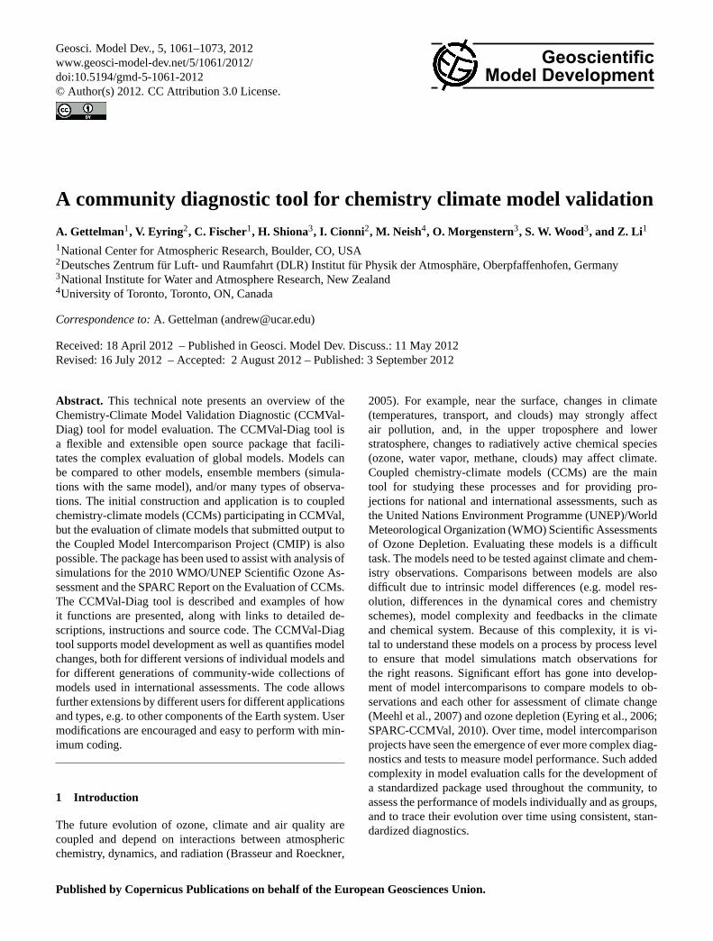
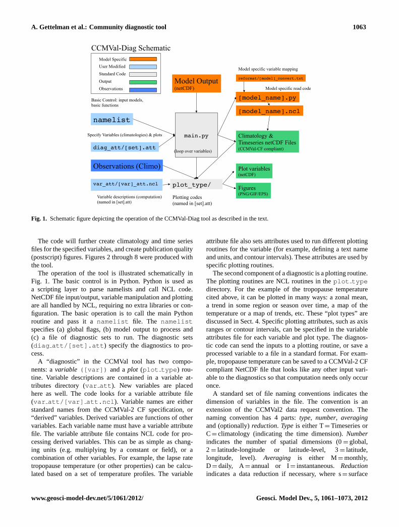
Fig. 1. Schematic figure depicting the operation of the CCMVal-Diag tool as described in thetext.

The code is set up to read in NetCDF files with either one time sample per file ormultiple time samples per file. It can also concatenate variables across multiple files.Examples of reading one and multiple time samples per file are contained in the sampleread code for CCSM.

8

Fig. 1. Schematic figure depicting the operation of the CCMVal-Diag tool as described in the text.

The code will further create climatology and time seriesfiles for the specified variables, and create publication quality(postscript) figures. Figures2 through8 were produced withthe tool.

The operation of the tool is illustrated schematically inFig. 1. The basic control is in Python. Python is used asa scripting layer to parse namelists and call NCL code.NetCDF file input/output, variable manipulation and plottingare all handled by NCL, requiring no extra libraries or con-figuration. The basic operation is to call the main Pythonroutine and pass it anamelist file. The namelistspecifies (a) global flags, (b) model output to process and(c) a file of diagnostic sets to run. The diagnostic sets(diag att/[set].att ) specify the diagnostics to pro-cess.

A “diagnostic” in the CCMVal tool has two compo-nents: avariable ([var]) and aplot (plot type ) rou-tine. Variable descriptions are contained in a variable at-tributes directory (var att ). New variables are placedhere as well. The code looks for a variable attribute file(var att/[var] att.ncl ). Variable names are eitherstandard names from the CCMVal-2 CF specification, or“derived” variables. Derived variables are functions of othervariables. Each variable name must have a variable attributefile. The variable attribute file contains NCL code for pro-cessing derived variables. This can be as simple as chang-ing units (e.g. multiplying by a constant or field), or acombination of other variables. For example, the lapse ratetropopause temperature (or other properties) can be calcu-lated based on a set of temperature profiles. The variable

attribute file also sets attributes used to run different plottingroutines for the variable (for example, defining a text nameand units, and contour intervals). These attributes are used byspecific plotting routines.

The second component of a diagnostic is a plotting routine.The plotting routines are NCL routines in theplot typedirectory. For the example of the tropopause temperaturecited above, it can be plotted in many ways: a zonal mean,a trend in some region or season over time, a map of thetemperature or a map of trends, etc. These “plot types” arediscussed in Sect.4. Specific plotting attributes, such as axisranges or contour intervals, can be specified in the variableattributes file for each variable and plot type. The diagnos-tic code can send the inputs to a plotting routine, or save aprocessed variable to a file in a standard format. For exam-ple, tropopause temperature can be saved to a CCMVal-2 CFcompliant NetCDF file that looks like any other input vari-able to the diagnostics so that computation needs only occuronce.

A standard set of file naming conventions indicates thedimension of variables in the file. The convention is anextension of the CCMVal2 data request convention. Thenaming convention has 4 parts:type, number, averagingand (optionally)reduction. Typeis either T= Timeseries orC= climatology (indicating the time dimension).Numberindicates the number of spatial dimensions (0= global,2 = latitude-longitude or latitude-level, 3= latitude,longitude, level). Averaging is either M= monthly,D = daily, A= annual or I= instantaneous.Reductionindicates a data reduction if necessary, where s= surface

www.geosci-model-dev.net/5/1061/2012/ Geosci. Model Dev., 5, 1061–1073, 2012


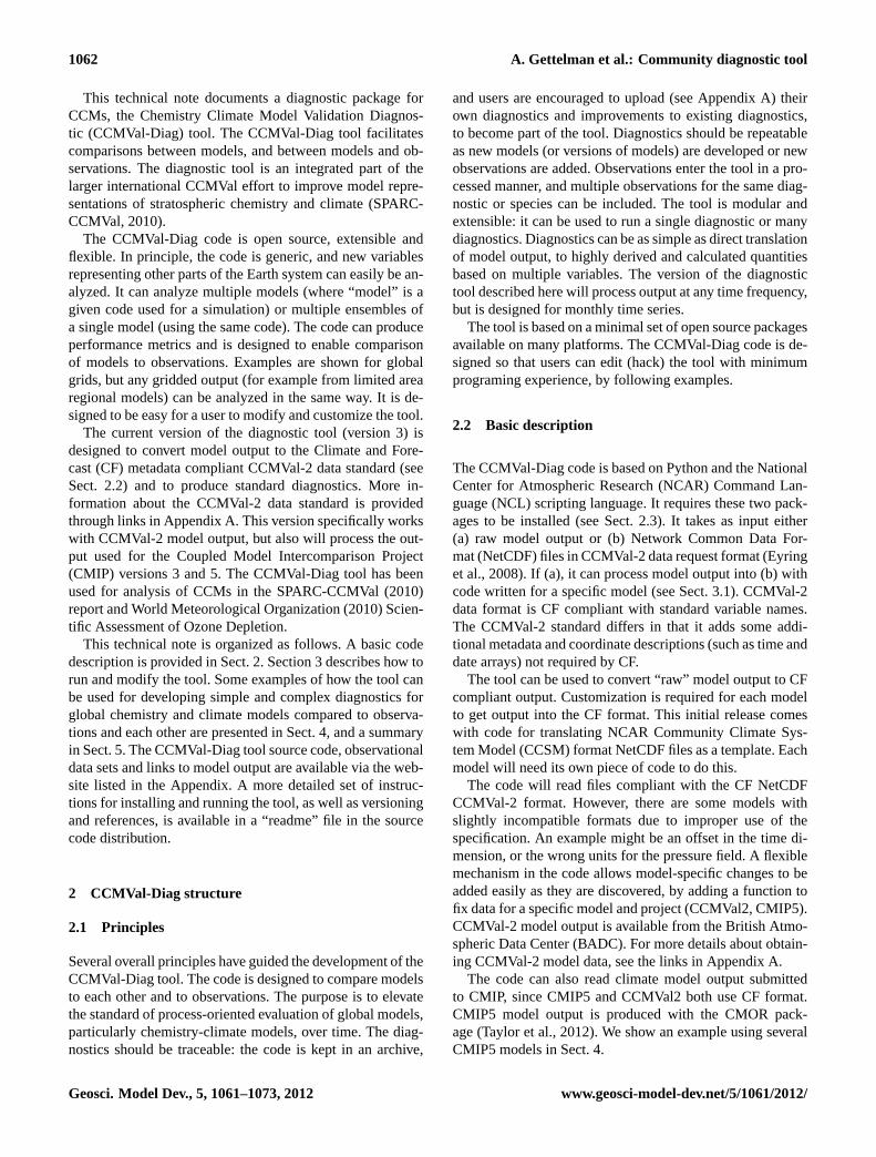
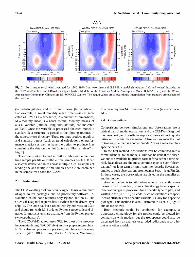
Fig. 2. Zonal mean zonal wind averaged for 1980–1990 from two historical (REF-B1) model simulations (left and center) included inthe CCMVal-2 archive and ERA40 reanalyses (right). Models are the Canadian Middle Atmosphere Model (CMAM-Left) and the WholeAtmosphere Community Climate Model (WACCM-Center). The height values are a logarithmic interpolation from standard atmosphere ofthe pressure.

(latitude-longitude) and z= zonal mean (latitude-level).For example, a zonal monthly mean time series is indi-cated as T2Mz (T= timeseries, 2= number of dimensions,M = monthly mean, z= zonal mean). Monthly means ofa 3-D variable (latitude, longitude, altitude) are indicatedas T3M. Once the variable is processed for each model, astandard data structure is passed to the plotting routines intheplot type directory. These routines produce graphicsand standard output (such as trend calculations or perfor-mance metrics) as well as have the option to produce filescontaining the data on the plot (noted as “Plot variables” inFig. 1).

The code is set up to read in NetCDF files with either onetime sample per file or multiple time samples per file. It canalso concatenate variables across multiple files. Examples ofreading one and multiple time samples per file are containedin the sample read code for CCSM.

2.3 Installation

The CCMVal-Diag tool has been designed to use a minimumof open source packages, and no proprietary software. In-stallation of the code requires only Python and NCL. TheCCMVal-Diag tool requires basic Python for the driver layer(Fig. 1). The code has been tested with Python version 2.3.4and should run with 2.3.4 or later. Python source code and bi-naries for most systems are available from the Python project(www.python.org).

The CCMVal-Diag tool uses NCL for most of its process-ing (manipulating NetCDF files) and for preparing graphics.NCL is also an open source package, with binaries for manysystems (AIX, IRIX, Linux, MacOSX, Solaris, Windows).

The code requires NCL version 5.1.0 or later (www.ncl.ucar.edu).

2.4 Observations

Comparisons between simulations and observations are acritical part of model evaluation, and the CCMVal-Diag toolhas been designed to easily incorporate observations in quali-tative and quantitative evaluation. Observations enter the toolin two ways: either as another “model” or as a separate plot-specific data file.

In the first method, observations can be converted into aformat identical to the models. This can be done if the obser-vations are available in gridded format for a defined time pe-riod. Reanalyses are the most common type of such “obser-vations”, or long-term or multi-satellite records. Several ex-amples of such observations are shown in Sect.4 (e.g. Fig.2).In these cases, the observations are listed in the namelist asanother model.

Another method is to tailor observations for specific com-parisons. In this method, often a climatology from a specificobservation type is processed for a specific type of plot, andwritten in theplot type code. Such observations are spec-ified as attributes for a specific variable, usually for a specificplot type. This method is also illustrated in Sect.4 (Figs.7and8; see below).

Both methods could be combined: for example, atropopause climatology for the tropics could be plotted forcomparison with models, but the tropopause could also becalculated from an analysis or gridded radiosonde record in-put as another model.


www.python.org

www.ncl.ucar.edu

www.ncl.ucar.edu


3 Processing methods

In this section, we describe the different processing methodsthat the CCMVal-Diag tool provides, and ways to use thetool.

3.1 Converting model output

In general, global models write data sequentially, with manyvariables for individual time samples, in files with single ormultiple time samples. For intercomparison projects, typi-cally files with multiple time samples and a single variableare desired to reduce output size, and for ease of processing.The CCMVal-Diag tool provides a framework and examplesfor processing of model output into correct formats for inter-comparisons. It can also be used to check formatting conven-tions. Currently, the most commonly used format is the CFcompliant NetCDF standard, and the tool is designed to readthis (and optionally write).

The CCMVal-Diag tool will process model output andgenerate two types of files: time series files (T3M, T2Ms, etc)which contain one variable at all times. The type specifica-tion follows the CCMVal-2 convention described earlier. Thecode also makes “climatology files” (C3M, etc) that are usedinternally for plotting, or in further post-processing. Time-series files are in CCMVal-2 CF compliant NetCDF format.

For processing of model files, the code requires 3 files (or-ange in Fig.1): (a) a Python driver to find the files, (b) anNCL code to process the files and (c) a text file to remapmodel variable names to CF compliant CCMVal-2 formatvariable names. The Python code (modelname.py ) setsthe filenames, gets the variable names, and then calls theNCL processing code (modelname.ncl ). The NCL pro-cessing code performs operations on the file list to concate-nate files together. For the initial conversion implementa-tion with the NCAR CCSM, the raw model output files areNetCDF files, but the structure will work on any other filetype that NCL can read. The user can supply NCL codeto read a specific raw model output in any format (binary,GRIB, HDF, ASCII, etc), and the tool will then process thefiles to CF compliant format. A utility for checking CF com-pliance is also included in the tool.

3.2 Comparing models to observations

Model comparisons to observations use one of the two meth-ods described in Sect. 2. Basically, these methods involvepre-processing the data to be interpreted as a separate model,or further processing to produce data directly for plotting.An example of the first type, data processed like a model,might be for a gridded satellite product, where 2-D (zonalor a surface) or 3-D monthly means can be produced in theCCMVal-2 format. Another example is a reanalysis data setsuch as the ERA40 reanalysis (Uppala et al., 2005) shown inFig. 2. Further examples are shown in Sect.4. The second

type would be a more heavily processed data set, read in fora specific variable and a specific plot. This could be an an-nual climatology file (monthly climatology of water vaporin 2-D or 3-D), such as used from the HALOE satellite inFig. 7. The diagnostic tool can even use specific values of aderived product (for example, meridional heat flux, definedas the product of anomalies of zonal wind (v′) and temper-ature (T ′)). These multiple methods allow flexibility. Bothmethods could be used in common for the same variable.

3.3 Comparing models to each other

In addition to comparing models to observations, theCCMVal-Diag tool is designed to compare models to eachother. The number of models is arbitrary. Model names (anda standard set of colors and line styles) for CCMVal mod-els have been included in the CCMVal-Diag tool, but modelswithout a known name will still be processed. The namesand number of models are simply read from the namelist.Each run or ensemble member is treated separately. Mul-tiple ensemble members from a single model can be pro-cessed. Each ensemble member can have different start andend dates. Some diagnostics require full years for process-ing. Many diagnostics can take a “reference” model (or ob-servation) for difference plots. Model output from differentscenarios can be placed on the same plot, such as a historicalrun and a future scenario, or two different future scenarios.The standard CCMVal-2 model set contains up to 18 models,some with ensemble members available.

Models can have their own grids (e.g. Fig.3). In principle,models need not have a full global grid either (limited areamodels can be processed). Difference plots interpolate andregrid for comparison purposes.

3.4 Quantitative trends and performance metrics

Several of the plotting routines are designed to plot time se-ries, and these plots also produce quantitative estimates oftrends. Trends can be calculated using any method desired.Currently, several of the routines provide trends based onlinear regression with significance testing, providing quanti-tative trends as well as confidence intervals. Trends can alsobe used as a diagnostic, for example plotting trends on a map(see Sect.4).

Another complex aspect of model intercomparison is pro-vided by the calculation of performance metrics. A perfor-mance metric is defined as a quantitative measure of agree-ment between a simulated and observed quantity, whichcan be used to assess the performance of individual mod-els (Knutti et al., 2010). These evaluations are complex, anddependent on the choice of diagnostics used. Several statis-tical measures for quantitative metrics comparing models toobservations have been built into the CCMVal-Diag tool forspecific purposes. An example is provided in Sect.4.3.



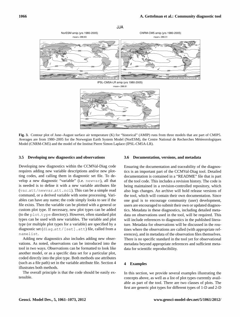
Fig. 3. Contour plot of June–August surface air temperature (K) for “historical” (AMIP) runs from three models that are part of CMIP5.Averages are from 1980–2005 for the Norwegian Earth System Model (NorESM), the Centre National de Recherches MeteeorologiquesModel (CNRM-CM5) and the model of the Institut Pierre Simon Laplace (IPSL-CM5A-LR).

3.5 Developing new diagnostics and observations

Developing new diagnostics within the CCMVal-Diag coderequires adding new variable descriptions and/or new plot-ting codes, and calling them in diagnostic set file. To de-velop a new diagnostic “variable” (i.e.newvar ), all thatis needed is to define it with a new variable attributes file(var att/newvar att.ncl ). This can be a simple readcommand, or a derived variable with some processing. Vari-ables can have any name; the code simply looks to see if thefile exists. Then the variable can be plotted with a general orcustom plot type. If necessary, new plot types can be added(to theplot type directory). However, often standard plottypes can be used with new variables. The variable and plottype (or multiple plot types for a variable) are specified by adiagnostic set (diag att/[set].att ) file, called from anamelist .

Adding new diagnostics also includes adding new obser-vations. As noted, observations can be introduced into thetool in two ways. Observations can be formatted to look likeanother model, or as a specific data set for a particular plot,coded directly into the plot type. Both methods use attributes(such as a file path) set in the variable attribute file. Section4illustrates both methods.

The overall principle is that the code should be easily ex-tensible.

3.6 Documentation, versions, and metadata

Ensuring the documentation and traceability of the diagnos-tics is an important part of the CCMVal-Diag tool. Detaileddocumentation is contained in a “README” file that is partof the tool code. This includes a revision history. The code isbeing maintained in a revision-controlled repository, whichalso logs changes. An archive will hold release versions ofthe tool, which will contain their own documentation. Sinceone goal is to encourage community (user) development,users are encouraged to submit their own or updated diagnos-tics. Metadata in these diagnostics, including detailed meta-data on observations used in the tool, will be required. Thiswill include references to diagnostics in the published litera-ture. Metadata for observations will be discussed in the rou-tines where the observations are called (with appropriate ref-erences), and in metadata of the observation files themselves.There is no specific standard in the tool yet for observationalmetadata beyond appropriate references and sufficient meta-data for scientific reproducibility.

4 Examples

In this section, we provide several examples illustrating theconcepts above, as well as a list of plot types currently avail-able as part of the tool. There are two classes of plots. Thefirst are generic plot types for different types of 1-D and 2-D



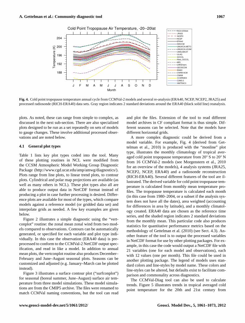
Fig. 4. Cold point tropopause temperature annual cycle from CCMVal-2 models and several re-analysis (ERA40, NCEP, NCEP2, JRA25) andprocessed radiosonde (RICH-ERA40) data sets. Gray region indicates 2 standard deviations around the ERA40 (black solid line) reanalysis.

plots. As noted, these can range from simple to complex, asdiscussed in the next sub-section. There are also specializedplots designed to be run as a set repeatedly on sets of modelsto gauge changes. These involve additional processed obser-vations and are noted below.

4.1 General plot types

Table 1 lists key plot types coded into the tool. Manyof these plotting routines in NCL were modified fromthe CCSM Atmospheric Model Working Group DiagnosticPackage (http://www.cgd.ucar.edu/amp/amwg/diagnostics/).Plots range from line plots, to linear trend plots, to contourplots. Cylindrical and polar map projections are available (aswell as many others in NCL). These plot types also all areable to produce output data in NetCDF format instead ofproducing a plot in case further processing is desired. Differ-ence plots are available for most of the types, which comparemodels against a reference model (or gridded data set) andinterpolate grids as needed. A few key examples are givenbelow.

Figure 2 illustrates a simple diagnostic using the “vert-conplot” routine: the zonal mean zonal wind from two mod-els compared to observations. Contours can be automaticallygenerated, or specified for each variable and plot type indi-vidually. In this case the observation (ERA40 data) is pre-processed to conform to the CCMVal-2 NetCDF output spec-ification, and read in like a model. In addition to annualmean plots, the vertconplot routine also produces December–February and June–August seasonal plots. Seasons can becustomized and adjusted (e.g. January–March can be plottedinstead).

Figure3 illustrates a surface contour plot (“surfconplot”)for seasonal (boreal summer, June–August) surface air tem-perature from three model simulations. These model simula-tions are from the CMIP5 archive. The files were renamed tomatch CCMVal naming conventions, but the tool can read

and plot the files. Extension of the tool to read differentmodel archives in CF compliant format is thus simple. Dif-ferent seasons can be selected. Note that the models havedifferent horizontal grids.

A more complex diagnostic could be derived from amodel variable. For example, Fig.4 (derived from Get-telman et al., 2010) is produced with the “monline” plottype, illustrates the monthly climatology of tropical aver-aged cold point tropopause temperature from 20◦ S to 20◦ Nfrom 16 CCMVal-2 models (seeMorgenstern et al., 2010for an overview of the models), 4 analysis systems (JRA25,NCEP2, NCEP, ERA40) and a radiosonde reconstruction(RICH-ERA40). Several different features of the tool are il-lustrated. The derived variable for cold point tropopause tem-perature is calculated from monthly mean temperature pro-files. The tropopause temperature is calculated each month(in this case from 1980–2004, or a subset if the analysis sys-tem does not have all the dates), area weighted (accountingfor differences in area by latitude), and a monthly climatol-ogy created. ERA40 data are chosen as the reference timeseries, and the shaded region indicates 2 standard deviationsfrom the monthly mean. This particular code also producesstatistics for quantitative performance metrics based on themethodology ofGettelman et al.(2010) (see Sect.4.3). An-other feature of the tool is to output the processed variablesin NetCDF format for use by other plotting packages. For ex-ample, in this case the code would output a NetCDF file with21 variables (one for each model and observations), eachwith 12 values (one per month). This file could be used inanother plotting package. The legend of models uses stan-dard colors and line-styles by model name. These colors andline-styles can be altered, but defaults exist to facilitate com-parison and commonality across diagnostics.

The CCMVal-Diag tool can also be used to calculatetrends. Figure5 illustrates trends in tropical averaged coldpoint temperature for the 20th and 21st century from


http://www.cgd.ucar.edu/amp/amwg/diagnostics/


Table 1.General plot types.

Plot Name Description

noplot no plot, convert onlysaveto netcdf save timeseries of a variableanncycplot annual cycle of monthly zonal meansvertconplot lat vs. height contour plot (3-D or 2-D zonal mean)plrconplot polar contour plot of a 2-D fieldseacycplot seasonal cycle line plot of seasonal cycleseadiffplot contour plot of seasonal difference DJF–JJAtsline timeseries plot: seasonal and annual, anomalies or full fieldmonline annual climatology plotssurfconplot 2-D surface contour plotsurfcontrend surface contour plot of trends at each pointzonlnplot zonal mean line plotzonlntrend zonal mean line plot of trendsprofiles vertical profiles at selected locations

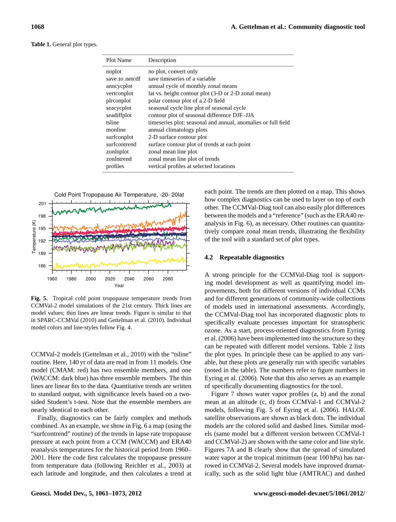
Fig. 5. Tropical cold point tropopause temperature trends fromCCMVal-2 model simulations of the 21st century. Thick lines aremodel values; thin lines are linear trends. Figure is similar to thatin SPARC-CCMVal(2010) andGettelman et al.(2010). Individualmodel colors and line-styles follow Fig.4.

CCMVal-2 models (Gettelman et al., 2010) with the “tsline”routine. Here, 140 yr of data are read in from 11 models. Onemodel (CMAM: red) has two ensemble members, and one(WACCM: dark blue) has three ensemble members. The thinlines are linear fits to the data. Quantitative trends are writtento standard output, with significance levels based on a two-sided Student’s t-test. Note that the ensemble members arenearly identical to each other.

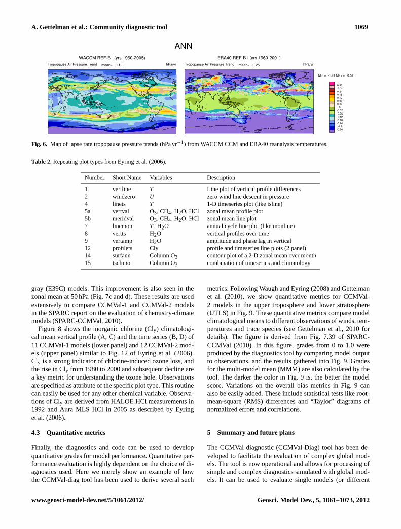
Finally, diagnostics can be fairly complex and methodscombined. As an example, we show in Fig.6a map (using the“surfcontrend” routine) of the trends in lapse rate tropopausepressure at each point from a CCM (WACCM) and ERA40reanalysis temperatures for the historical period from 1960–2001. Here the code first calculates the tropopause pressurefrom temperature data (followingReichler et al., 2003) ateach latitude and longitude, and then calculates a trend at

each point. The trends are then plotted on a map. This showshow complex diagnostics can be used to layer on top of eachother. The CCMVal-Diag tool can also easily plot differencesbetween the models and a “reference” (such as the ERA40 re-analysis in Fig.6), as necessary. Other routines can quantita-tively compare zonal mean trends, illustrating the flexibilityof the tool with a standard set of plot types.

4.2 Repeatable diagnostics

A strong principle for the CCMVal-Diag tool is support-ing model development as well as quantifying model im-provements, both for different versions of individual CCMsand for different generations of community-wide collectionsof models used in international assessments. Accordingly,the CCMVal-Diag tool has incorporated diagnostic plots tospecifically evaluate processes important for stratosphericozone. As a start, process-oriented diagnostics fromEyringet al.(2006) have been implemented into the structure so theycan be repeated with different model versions. Table2 liststhe plot types. In principle these can be applied to any vari-able, but these plots are generally run with specific variables(noted in the table). The numbers refer to figure numbers inEyring et al.(2006). Note that this also serves as an exampleof specifically documenting diagnostics for the tool.

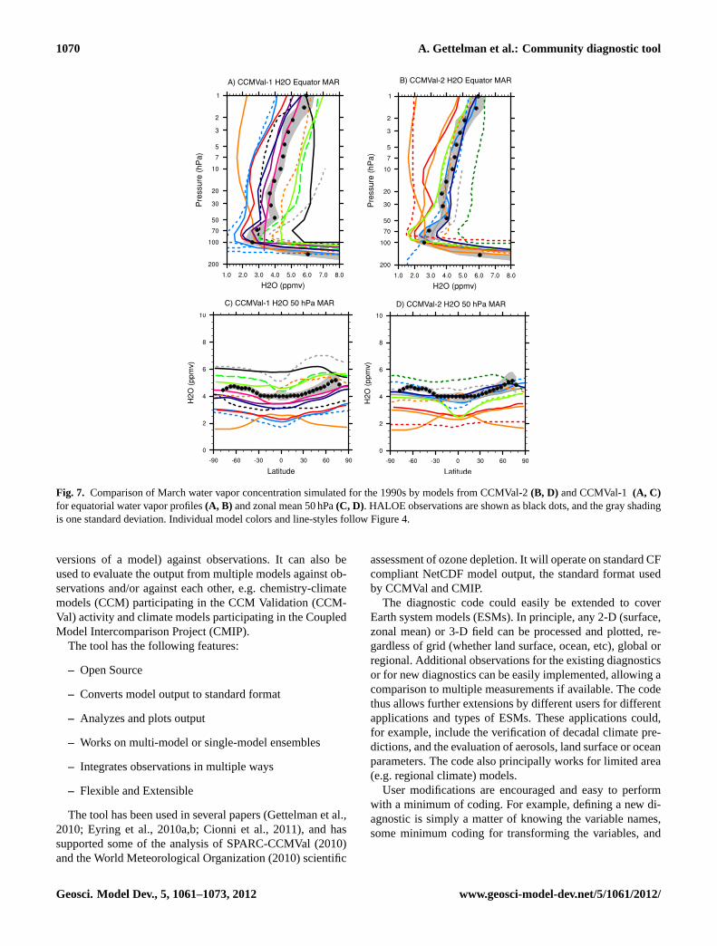
Figure7 shows water vapor profiles (a, b) and the zonalmean at an altitude (c, d) from CCMVal-1 and CCMVal-2models, following Fig. 5 ofEyring et al.(2006). HALOEsatellite observations are shown as black dots. The individualmodels are the colored solid and dashed lines. Similar mod-els (same model but a different version between CCMVal-1and CCMVal-2) are shown with the same color and line style.Figures7A and B clearly show that the spread of simulatedwater vapor at the tropical minimum (near 100 hPa) has nar-rowed in CCMVal-2. Several models have improved dramat-ically, such as the solid light blue (AMTRAC) and dashed



Fig. 6. Map of lapse rate tropopause pressure trends (hPa yr−1) from WACCM CCM and ERA40 reanalysis temperatures.

Table 2.Repeating plot types fromEyring et al.(2006).

Number Short Name Variables Description

1 vertline T Line plot of vertical profile differences2 windzero U zero wind line descent in pressure4 linets T 1-D timeseries plot (like tsline)5a vertval O3, CH4, H2O, HCl zonal mean profile plot5b meridval O3, CH4, H2O, HCl zonal mean line plot7 linemon T , H2O annual cycle line plot (like monline)8 vertts H2O vertical profiles over time9 vertamp H2O amplitude and phase lag in vertical12 profilets Cly profile and timeseries line plots (2 panel)14 surfann Column O3 contour plot of a 2-D zonal mean over month15 tsclimo Column O3 combination of timeseries and climatology

gray (E39C) models. This improvement is also seen in thezonal mean at 50 hPa (Fig.7c and d). These results are usedextensively to compare CCMVal-1 and CCMVal-2 modelsin the SPARC report on the evaluation of chemistry-climatemodels (SPARC-CCMVal, 2010).

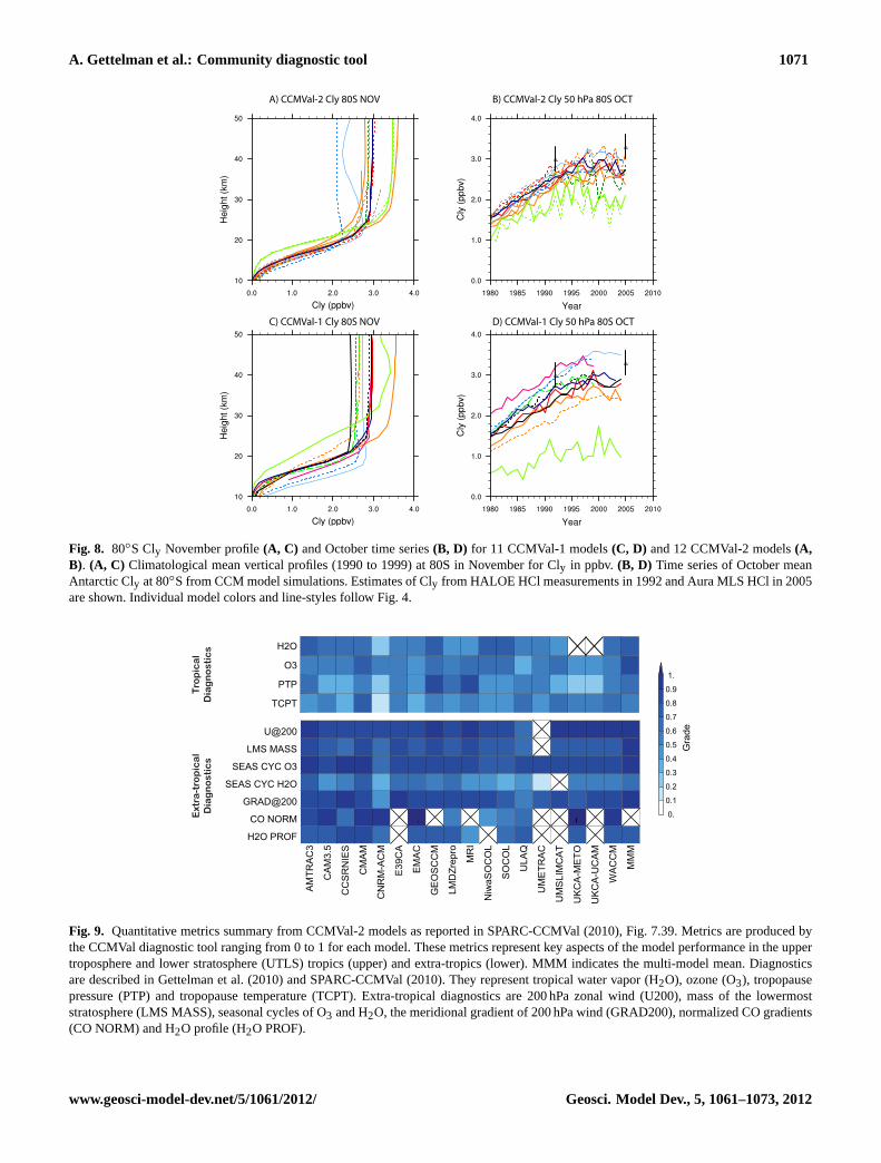
Figure8 shows the inorganic chlorine (Cly) climatologi-cal mean vertical profile (A, C) and the time series (B, D) of11 CCMVal-1 models (lower panel) and 12 CCMVal-2 mod-els (upper panel) similar to Fig. 12 ofEyring et al.(2006).Cly is a strong indicator of chlorine-induced ozone loss, andthe rise in Cly from 1980 to 2000 and subsequent decline area key metric for understanding the ozone hole. Observationsare specified as attribute of the specific plot type. This routinecan easily be used for any other chemical variable. Observa-tions of Cly are derived from HALOE HCl measurements in1992 and Aura MLS HCl in 2005 as described byEyringet al.(2006).

4.3 Quantitative metrics

Finally, the diagnostics and code can be used to developquantitative grades for model performance. Quantitative per-formance evaluation is highly dependent on the choice of di-agnostics used. Here we merely show an example of howthe CCMVal-diag tool has been used to derive several such

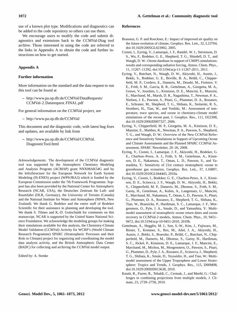
metrics. FollowingWaugh and Eyring(2008) andGettelmanet al. (2010), we show quantitative metrics for CCMVal-2 models in the upper troposphere and lower stratosphere(UTLS) in Fig.9. These quantitative metrics compare modelclimatological means to different observations of winds, tem-peratures and trace species (seeGettelman et al., 2010 fordetails). The figure is derived from Fig. 7.39 ofSPARC-CCMVal (2010). In this figure, grades from 0 to 1.0 wereproduced by the diagnostics tool by comparing model outputto observations, and the results gathered into Fig.9. Gradesfor the multi-model mean (MMM) are also calculated by thetool. The darker the color in Fig.9 is, the better the modelscore. Variations on the overall bias metrics in Fig.9 canalso be easily added. These include statistical tests like root-mean-square (RMS) differences and “Taylor” diagrams ofnormalized errors and correlations.

5 Summary and future plans

The CCMVal diagnostic (CCMVal-Diag) tool has been de-veloped to facilitate the evaluation of complex global mod-els. The tool is now operational and allows for processing ofsimple and complex diagnostics simulated with global mod-els. It can be used to evaluate single models (or different



A) CCMVal-1 H2O Equator MAR B) CCMVal-2 H2O Equator MAR

C) CCMVal-1 H2O 50 hPa MAR D) CCMVal-2 H2O 50 hPa MAR

Fig. 7. Comparison of March water vapor concentration simulated for the 1990s by models from CCMVal-2(B, D) and CCMVal-1 (A, C)for equatorial water vapor profiles(A, B) and zonal mean 50 hPa(C, D). HALOE observations are shown as black dots, and the gray shadingis one standard deviation. Individual model colors and line-styles follow Figure4.

versions of a model) against observations. It can also beused to evaluate the output from multiple models against ob-servations and/or against each other, e.g. chemistry-climatemodels (CCM) participating in the CCM Validation (CCM-Val) activity and climate models participating in the CoupledModel Intercomparison Project (CMIP).

The tool has the following features:

– Open Source

– Converts model output to standard format

– Analyzes and plots output

– Works on multi-model or single-model ensembles

– Integrates observations in multiple ways

– Flexible and Extensible

The tool has been used in several papers (Gettelman et al.,2010; Eyring et al., 2010a,b; Cionni et al., 2011), and hassupported some of the analysis ofSPARC-CCMVal(2010)and theWorld Meteorological Organization(2010) scientific

assessment of ozone depletion. It will operate on standard CFcompliant NetCDF model output, the standard format usedby CCMVal and CMIP.

The diagnostic code could easily be extended to coverEarth system models (ESMs). In principle, any 2-D (surface,zonal mean) or 3-D field can be processed and plotted, re-gardless of grid (whether land surface, ocean, etc), global orregional. Additional observations for the existing diagnosticsor for new diagnostics can be easily implemented, allowing acomparison to multiple measurements if available. The codethus allows further extensions by different users for differentapplications and types of ESMs. These applications could,for example, include the verification of decadal climate pre-dictions, and the evaluation of aerosols, land surface or oceanparameters. The code also principally works for limited area(e.g. regional climate) models.

User modifications are encouraged and easy to performwith a minimum of coding. For example, defining a new di-agnostic is simply a matter of knowing the variable names,some minimum coding for transforming the variables, and



A) CCMVal-2 Cly 80S NOV B) CCMVal-2 Cly 50 hPa 80S OCT

C) CCMVal-1 Cly 80S NOV D) CCMVal-1 Cly 50 hPa 80S OCT

Fig. 8. 80◦S Cly November profile(A, C) and October time series(B, D) for 11 CCMVal-1 models(C, D) and 12 CCMVal-2 models(A,B). (A, C) Climatological mean vertical profiles (1990 to 1999) at 80S in November for Cly in ppbv. (B, D) Time series of October meanAntarctic Cly at 80◦S from CCM model simulations. Estimates of Cly from HALOE HCl measurements in 1992 and Aura MLS HCl in 2005are shown. Individual model colors and line-styles follow Fig.4.

0.

0.1

0.2

0.3

0.4

0.5

0.6

0.7

0.8

0.9

1.G

rade

TCPT

PTP

O3

H2O

. 1

AM

TRA

C3

CA

M3.

5

CC

SR

NIE

S

CM

AM

CN

RM

-AC

M

E39

CA

EM

AC

GE

OS

CC

M

LMD

Zrep

ro

MR

I

Niw

aSO

CO

L

SO

CO

L

ULA

Q

UM

ETR

AC

UM

SLI

MC

AT

UK

CA

-ME

TO

UK

CA

-UC

AM

WA

CC

M

MM

M

H2O PROF

CO NORM

GRAD@200

SEAS CYC H2O

SEAS CYC O3

LMS MASS

U@200

Tro

pical

Diagnostics

Extra

-tro

pical

Diagnostics

Fig. 9. Quantitative metrics summary from CCMVal-2 models as reported inSPARC-CCMVal(2010), Fig. 7.39. Metrics are produced bythe CCMVal diagnostic tool ranging from 0 to 1 for each model. These metrics represent key aspects of the model performance in the uppertroposphere and lower stratosphere (UTLS) tropics (upper) and extra-tropics (lower). MMM indicates the multi-model mean. Diagnosticsare described inGettelman et al.(2010) andSPARC-CCMVal(2010). They represent tropical water vapor (H2O), ozone (O3), tropopausepressure (PTP) and tropopause temperature (TCPT). Extra-tropical diagnostics are 200 hPa zonal wind (U200), mass of the lowermoststratosphere (LMS MASS), seasonal cycles of O3 and H2O, the meridional gradient of 200 hPa wind (GRAD200), normalized CO gradients(CO NORM) and H2O profile (H2O PROF).



use of a known plot type. Modifications and diagnostics canbe added to the code repository so others can use them.

We encourage users to modify the code and submit di-agnostics and extensions back to the CCMVal-Diag toolarchive. Those interested in using the code are referred tothe links in Appendix A to obtain the code and further in-structions on how to get started.

Appendix A

Further information

More information on the standard and the data request to runthis tool can be found at

– http://www.pa.op.dlr.de/CCMVal/DataRequests/CCMVal-2 DatarequestFINAL.pdf

For general information on the CCMVal project, see

– http://www.pa.op.dlr.de/CCMVal/

This document and the diagnostic code, with latest bug fixesand updates, are available by link from

– http://www.pa.op.dlr.de/CCMVal/CCMValDiagnosticTool.html

Acknowledgements.The development of the CCMVal diagnostictool was supported by the Atmospheric Chemistry Modelingand Analysis Program (ACMAP) grant NNX08AK54G and bythe InfraStructure for the European Network for Earth SystemModeling (IS-ENES) project (WP9/JRA3) which is funded by theEuropean Commission under the 7th Framework Programme. Sup-port has also been provided by the National Center for AtmosphericResearch (NCAR, USA), the Deutsches Zentrum fur Luft- undRaumfahrt (DLR, Germany), the University of Toronto (Canada)and the National Institute for Water and Atmosphere (NIWA, NewZealand). We thank G. Bodeker and the entire staff of BodekerScientific for their assistance in planning and developing the tool.We thank S. Tilmes and K.-D. Gottschaldt for comments on thismanuscript. NCAR is supported by the United States National Sci-ence Foundation. We acknowledge the modeling groups for makingtheir simulations available for this analysis, the Chemistry-ClimateModel Validation (CCMVal) Activity for WCRP’s (World ClimateResearch Programme) SPARC (Stratospheric Processes and theirRole in Climate) project for organizing and coordinating the modeldata analysis activity, and the British Atmospheric Data Center(BADC) for collecting and archiving the CCMVal model output.

Edited by: A. Stenke

References

Brasseur, G. P. and Roeckner, E.: Impact of improved air quality onthe future evolution of climate, Geophys. Res. Lett., 32, L23704,doi:10.1029/2005GL023902, 2005.

Cionni, I., Eyring, V., Lamarque, J. F., Randel, W. J., Stevenson, D.S., Wu, F., Bodeker, G. E., Shepherd, T. G., Shindell, D. T., andWaugh, D. W.: Ozone database in support of CMIP5 simulations:results and corresponding radiative forcing, Atmos. Chem. Phys.,11, 11267–11292,doi:10.5194/acp-11-11267-2011, 2011.

Eyring, V., Butchart, N., Waugh, D. W., Akiyoshi, H., Austin, J.,Bekki, S., Bodeker, G. E., Boville, B. A., Bruhl, C., Chipper-field, M. P., Cordero, E., Dameris, M., Deushi, M., Fioletov, V.E., Frith, S. M., Garcia, R. R., Gettelman, A., Giorgetta, M. A.,Grewe, V., Jourdain, L., Kinnison, D. E., Mancini, E., Manzini,E., Marchand, M., Marsh, D. R., Nagashima, T., Newman, P. A.,Nielsen, J. E., Pawson, S., Pitari, G., Plummer, D. A., Rozanov,E., Schraner, M., Shepherd, T. G., Shibata, K., Stolarski, R. S.,Struthers, H., Tian, W., and Yoshiki, M.: Assessment of tem-perature, trace species, and ozone in chemistry-climate modelsimulations of the recent past, J. Geophys. Res., 111, D22308,doi:10.1029/2006JD007327, 2006.

Eyring, V., Chipperfield, M. P., Giorgetta, M. A., Kinnison, D. E.,Manzini, E., Matthes, K., Newman, P. A., Pawson, S., Shepherd,T. G., and Waugh, D. W.: Overview of the New CCMVal Refer-ence and Sensitivity Simulations in Support of Upcoming Ozoneand Climate Assessments and the Planned SPARC CCMVal As-sessment, SPARC Newsletter, 20–26, 2008.

Eyring, V., Cionni, I., Lamarque, J. F., Akiyoshi, H., Bodeker, G.E., Charlton–Perez, A. J., Frith, S. M., Gettelman, A., Kinni-son, D. E., Nakamura, T., Oman, L. D., Pawson, S., and Ya-mashita, Y.: Sensitivity of 21st century stratospheric ozone togreenhouse gas scenarios, Geophys. Res. Lett., 37, L16807,doi:10.1029/2010GL044443, 2010a.

Eyring, V., Cionni, I., Bodeker, G. E., Charlton-Perez, A. J., Kinni-son, D. E., Scinocca, J. F., Waugh, D. W., Akiyoshi, H., Bekki,S., Chipperfield, M. P., Dameris, M., Dhomse, S., Frith, S. M.,Garny, H., Gettelman, A., Kubin, A., Langematz, U., Mancini,E., Marchand, M., Nakamura, T., Oman, L. D., Pawson, S., Pitari,G., Plummer, D. A., Rozanov, E., Shepherd, T. G., Shibata, K.,Tian, W., Braesicke, P., Hardiman, S. C., Lamarque, J. F., Mor-genstern, O., Pyle, J. A., Smale, D., and Yamashita, Y.: Multi-model assessment of stratospheric ozone return dates and ozonerecovery in CCMVal-2 models, Atmos. Chem. Phys., 10, 9451–9472,doi:10.5194/acp-10-9451-2010, 2010b.

Gettelman, A., Hegglin, M. I., Son, S.-W., Kim, J., Fujiwara, M.,Birner, T., Kremser, S., Rex, M., Anel, J. A., Akiyoshi, H.,Austin, J., Bekki, S., Braesike, P., Bruhl, C., Butchart, N., Chip-perfield, M., Dameris, M., Dhomse, S., Garny, H., Hardiman,S. C., Jockel, P., Kinnison, D. E., Lamarque, J. F., Mancini, E.,Marchand, M., Michou, M., Morgenstern, O., Pawson, S., Pitari,G., Plummer, D., Pyle, J. A., Rozanov, E., Scinocca, J., Shepherd,T. G., Shibata, K., Smale, D., Teyssedre, H., and Tian, W.: Multi-model assessment of the Upper Troposphere and Lower Strato-sphere: Tropics and Trends, J. Geophys. Res., 115, D00M08,doi:10.1029/2009JD013638, 2010.

Knutti, R., Furrer, R., Tebaldi, C., Cermak, J., and Meehl, G.: Chal-lenges in combining projections from multiple models, J. Cli-mate, 23, 2739–2758, 2010.


http://www.pa.op.dlr.de/CCMVal/DataRequests/CCMVal-2_Datarequest_FINAL.pdf

http://www.pa.op.dlr.de/CCMVal/DataRequests/CCMVal-2_Datarequest_FINAL.pdf

http://www.pa.op.dlr.de/CCMVal/

http://www.pa.op.dlr.de/CCMVal/CCMVal_DiagnosticTool.html

http://www.pa.op.dlr.de/CCMVal/CCMVal_DiagnosticTool.html

http://dx.doi.org/10.1029/2005GL023902

http://dx.doi.org/10.5194/acp-11-11267-2011

http://dx.doi.org/10.1029/2006JD007327

http://dx.doi.org/10.1029/2010GL044443


http://dx.doi.org/10.1029/2009JD013638


Meehl, G. A., Covey, C., Taylor, K. E., Delworth, T., Stouffer,R. J., Latif, M., McAvaney, B., and Mitchell, J. F. B.: TheWCRP CMIP3 Multimodel Dataset: A New Era in ClimateChange Research, Bull. Am. Meteorol. Soc., 88, 1383–1394,doi:10.1175/BAMS-88-9-1383, 2007.

Morgenstern, O., Giorgetta, M. A., Shibata, K., Eyring, V., Waugh,D. W., Shepherd, T. G., Akiyoshi, H., Austin, J., Baumgaertner,A. J. G., Bekki, S., Braesicke, P., Br¸hl, C., Chipperfield, M. P.,Cugnet, D., Dameris, M., Dhomse, S., Frith, S. M., Garny, H.,Gettelman, A., Hardiman, S. C., Hegglin, M. I., Jockel, P., Kinni-son, D. E., Lamarque, J.-F., Mancini, E., Manzini, E., Marchand,M., Michou, M., Nakamura, T., Nielsen, J. E., Olivie, D., Pitari,G., Plummer, D. A., Rozanov, E., Scinocca, J. F., Smale, D.,Teyssedre, H., Toohey, M., Tian, W., and Yamashita, Y.: Reviewof the formulation of present-generation stratospheric chemistry-climate models and associated external forcings, J. Geophys.Res., 115, D00M02,doi:10.1029/2009JD013728, 2010.

Reichler, T., Dameris, M., and Sausen, R.: Determination of theTropopause Height from gridded data, Geophys. Res. Lett., 30,2042,doi:10.1029/2003GL018240, 2003.

SPARC-CCMVal: SPARC Report on the Evaluation of Chemistry-Climate Models, SPARC Report 5, WCRP-132, WMO/TD-1526, Stratospheric Processes and Their Role In Climate, WorldMeteorological Organization, 2010.

Taylor, K. E., Stouffer, R. J., and Meehl, G. A.: An Overview ofCMIP5 and the Experimental Design, in press, Bull. Amer. Met.Soc, 93, 485–498,doi:10.1175/BAMS-D-11-00094.1, 2012.

Uppala, S., Kallberg, P., Simmons, A., Andrae, U., da Costa Bech-told, V., Fiorino, M., Gibson, J., Haseler, J., Hernandez, A., Kelly,G., Li, X., Onogi, K., Saarinen, S., Sokka, N., Allan, R., Ander-sson, E., Arpe, K., Balmaseda, M., Beljaars, A., van de Berg,L., Bidlot, J., Bormann, N., Caires, S., Chevallier, F., Dethof, A.,Dragosavac, M., Fisher, M., Fuentes, M., Hagemann, S., Holm,E., Hoskins, B., Isaksen, L., Janssen, P., Jenne, R., McNally, A.,Mahfouf, J.-F., Morcrette, J.-J., Rayner, N., Saunders, R., Simon,P., Sterl, A., Trenberth, K., Untch, A., Vasiljevic, D., Viterbo,P., and Woollen, J.: The ERA-40 re-analysis, Q. J. R. Meteorol.Soc., 131, 2961–3012, 2005.

Waugh, D. W. and Eyring, V.: Quantitative performance met-rics for stratospheric-resolving chemistry-climate models, At-mos. Chem. Phys., 8, 5699–5713,doi:10.5194/acp-8-5699-2008,2008.

World Meteorological Organization: Scientific Assessment ofOzone Depletion: 2010, WMO Report, World MeteorologicalOrganization, Geneva, 2010.


http://dx.doi.org/10.1175/BAMS-88-9-1383

http://dx.doi.org/10.1029/2009JD013728

http://dx.doi.org/10.1029/2003GL018240

http://dx.doi.org/10.1175/BAMS-D-11-00094.1


Documents

A community diagnostic tool for chemistry climate model