HAL Id: hal-01735695https://hal.archives-ouvertes.fr/hal-01735695

Submitted on 16 Mar 2018

HAL is a multi-disciplinary open accessarchive for the deposit and dissemination of sci-entific research documents, whether they are pub-lished or not. The documents may come fromteaching and research institutions in France orabroad, or from public or private research centers.

L’archive ouverte pluridisciplinaire HAL, estdestinée au dépôt et à la diffusion de documentsscientifiques de niveau recherche, publiés ou non,émanant des établissements d’enseignement et derecherche français ou étrangers, des laboratoirespublics ou privés.

A Combined Experimental and Numerical Investigationof the Flow and Heat Transfer Inside a Turbine Vane

Cooled by Jet ImpingementEmmanuel Laroche, Matthieu Fénot, Eva Dorignac, Jean-Jacques Vuillerme,

Laurent-Emmanuel Brizzi, Juan Larroya

To cite this version:Emmanuel Laroche, Matthieu Fénot, Eva Dorignac, Jean-Jacques Vuillerme, Laurent-EmmanuelBrizzi, et al.. A Combined Experimental and Numerical Investigation of the Flow and Heat TransferInside a Turbine Vane Cooled by Jet Impingement. Journal of Turbomachinery, American Society ofMechanical Engineers, 2017, 140 (3), pp.031002. �10.1115/1.4038411�. �hal-01735695�

1

A combined experimental and numerical investigation of the flow and heat transfer

inside a turbine vane cooled by jet impingement

Emmanuel Laroche1 ONERA, The French Aerospace Lab F31055, Toulouse, France emmanuel.laroche@onera.fr Matthieu Fenot PPRIME Institute Chasseneuil Futuroscope, France Eva Dorignac PPRIME Institute Chasseneuil Futuroscope, France Jean-Jacques Vuillerme PPRIME Institute Chasseneuil Futuroscope, France Laurent Emmanuel Brizzi PPRIME Institute Chasseneuil Futuroscope, France Juan Carlos Larroya Safran Aircraft Engines Moissy Cramayel, France ABSTRACT

The present study aims at characterizing the flow field and heat transfer for a schematic but realistic vane

cooling scheme. Experimentally, both velocity and heat transfer measurements are conducted to provide a

.

2

detailed database of the investigated configuration. From a numerical point of view, the configuration is

investigated using isotropic as well as anisotropic Reynolds-Averaged Navier-Stokes (RANS) turbulence

models. An hybrid RANS/LES technique is also considered to evaluate potential unsteady effects. Both

experimental and numerical results show a very complex 3D flow. Air is not evenly distributed between

the different injections, mainly because of a large recirculation flow. Due to the strong flow deviation at

the hole inlet, the velocity distribution and the turbulence characteristics at the hole exit are far from fully

developed profiles. The comparison between PIV measurements and numerical results shows a reasonable

agreement. However, coming to heat transfer, all RANS models exhibit a major overestimation compared

to IR thermography measurements. The Billard-Laurence model does not bring any improvement

compared to a classical k-ω SST model. The hybrid RANS/LES simulation provides the best heat transfer

estimation, exhibiting potential unsteady effects ignored by RANS models. Those conclusions are different

from the ones usually obtained for a single fully developed impinging jet.

INTRODUCTION

In today’s engines inlet turbine gas temperature largely exceeds blade material

melting temperature. As a result, cooling techniques are essential to maintain blades at

a reasonable temperature. A satisfactory understanding of these techniques is crucial to

achieve optimum heat transfer while minimizing the coolant flow rate. With film

cooling, jet impingement is one of the most frequently used techniques for turbine

blade cooling. It is especially introduced where the thermal conditions are the most

severe: the nozzle guide vane, the leading edge and midspan regions of the vanes. In

spite of their apparent simplicity, impinging jets reveal a complex dynamic, which is

responsible for an intensive heat transfer rate. To optimize this process, a detailed

knowledge of the flow mechanisms (in particular in the near wall flow structures) and of

3

the thermal interaction between the fluid and the wall is required. Consequently, many

studies have been conducted on the visualization, qualification and comprehension of

jet flow structures and heat transfer. Martin[1], Jambunathan et al.[2], Viskanta [3] and

Zukerman and Lior[4] have reviewed a large panel of jet impingement studies. The most

widely studied configuration is a single jet issuing from a long tube or from a contraction

nozzle. For such “academic” configurations, an impinging jet can be divided into three

zones: the free jet, the stagnation zone and the wall jet. The free jet is itself constituted

of a potential core (low turbulent region) surrounded by a shear layer with roll–up

vortices. Close to the wall, the jet enters the stagnation zone. In this zone, jet flow is

turned radially outward. Mixing layer vortices are deflected and roll along the impinging

plate. Resulting heat transfer has been measured and studied by many authors ([5-7])

with a maximum around the impinging point and then a decrease. Coming to the issue

of multi-array impingement cooling, the numerous studies are summarized in a review

paper by Weigand and Spring [8], investigating such effects as crossflow or jet/jet

interaction. Earlier, Florschuetz et al provided correlations for uniform and staggered jet

arrangements [9].

But such jets and heat transfer rates could be very different from those

encountered in vane cooling systems principally because of the impinged plate

curvature and of the injection flow feeding: impinging jets are typically generated with a

thin perforated plate inserted into the vane and pressurized with air. Air is injected

through the perforations and impinges on the vane inner surface. Very few studies have

been conducted on such a jet ([10]) and none, to our knowledge, have taken into

4

account all parameters encountered in a vane (injection feeding, multiple jets,

curvature). The purpose of the present study is to investigate the flow and heat transfer

for a large scale vane cooling scheme. Both flow and heat transfer have been measured

experimentally and compared to numerical simulations. The chosen configuration

corresponds to a global mass flow rate that provides a mean Reynolds number value of

10000 in each hole.

EXPERIMENTAL SET-UP AND MEASUREMENTS

Experimental facility

The experimental facility is shown in Figure 1. The air flow is supplied by a fan,

and passes through a heat exchanger to control its temperature throughout the

experiment (maintained equal to 20°C). A valve regulates the global air flow rate and a

venturi meter allows to measure the mass flow. The venturi meter and associated

pressure converters had previously been calibrated over the mass flow rate range of the

experiment (up to 60 g/s). The airflow goes through a divergent passage and enters the

central cavity of the test section which is presented in Figure 2.

The test section is divided in two parts: the central cavity that feeds the different

holes and the impingement plate which represents the blade wall. The central cavity is a

rectangular channel, 400mm large, 250mm long and 20mm high made of altuglas. A

semi cylinder closes the channel on the leading side. Three rows of five D1=10mm

diameter holes are drilled through upper and lower part (representing pressure and

suction sides). A row of nine larger holes (D2 diameter equal to 1.25 D1=12.5mm) are

5

made through its semi cylinder part. The injection plate thickness is equal to 10mm for

all the holes.

Two different impingement plates are used depending on the measurement

technique. For velocity measurement, the impingement plate is made of altuglas to

allow optical access. For heat transfer measurement, jets impinge on a 0.4 mm epoxy-

glass plate covered on the impinging side with a thin copper foil. The thickness of the

copper foil is 35μm and it is engraved by a circuit that is linked to a DC supply and allows

heating of the plate by Joule effect. The back of the impingement plate is painted in

black to ensure high uniform emissivity (ε=0.95) to allow a rigorous estimation of

radiative heat fluxes and heat transfer measurements. An infrared camera (CEDIP

titanium) measures the backward temperature of the plate. To cover the whole plate,

21 images are recorded. The junctions between them correspond to low emissivity

marks which will be visualized later on the heat transfer distribution under the form of

white disks.

Jets injection mass flow measurement

Only the global mass flow rate is measured and controlled through the valve and

the venturi meter seen on Figure 1. However, due to the relative small size of the

central cavity, the flow distribution is heterogeneous between the 39 holes. To estimate

the ratio between the different injection holes, a specific experiment has been

conducted. Considering that the impinged plate has no influence over the injection flow

6

for an injection-to-plate distance superior to 1 injection diameter [11], the impinged

plate was removed and 39 identical venturi meters were added at the exit of each hole,

allowing us to measure injection mass flow rate individually.

Velocity measurement

Particle image velocimetry was used to measure and calculate mean and RMS

velocity fields. Flow seeding was achieved with a smoke atomizer producing water and

glycerin particles which mean diameter is inferior to 1 μm. Those particles were injected

directly into the fan. The flow was illuminated by a Yag pulsed Laser. Resulting light

sheet thickness is inferior to 1.5 mm. Images were acquired with a 1008x1014 px²

HiSense camera with a sampling frequency of 4.5Hz for all measurements.

To ensure accurate statistics, we record a total number of velocity fields superior

to 1000 for each measurement. Velocities were estimated using Davis software. A three

step adaptive cross-correlation was used (initial pass 64x64, final pass 32x32 doubled,

50% overlap). Validation steps are carried out in an effort to eliminate erroneous

velocity vectors: only vectors with a signal/noise ratio of 1.5 are validated and 500

validated vectors are needed to take a result into account.

To understand the very complex topology of the flow field, velocity

measurements have been performed in different planes presented in Figure 3 (named

(A) to (D)).

Heat transfer measurement

7

The method used to determine the heat transfer coefficient has already been

presented in various papers ([6-10]). Considering the Newton's law of cooling:

( 1 )

With ϕconv , the convective heat flux density on the impinged side, Tw, the wall

temperature and Tref, the reference temperature. The method consists in prescribing

different convective heat flux densities ϕconv and in measuring the wall temperature Tw

at a given location of the impinged plate for each. Then, 1/h is identified as the slope

and Tref as the y-intercept of a straight line linking each couple (ϕconv, Tw) as seen in

Figure 4. In practical terms, ϕconv is prescribed using the copper circuit described above.

A uniform electrical flux density is produced by Joule effect. Radiative losses on both

sides and convective losses on the back side (opposite the impinged side) are calculated

and deduced from the electrical flux to determine ϕconv. The sum of those losses is less

than 15% of electrical heat flux. After thermal equilibrium is reached, temperature is

recorded on the back side of the plate using an infrared camera. By repeating this

procedure four times for each position with different electrical flux densities (from

500W/m² to 2000W/m²), we can deduce the cartographies of local convective heat

transfer coefficient h and reference temperature Tref. Uncertainties were calculated

using the statistical approach based on Coleman and Steele [12]. Taking into account

errors due to ambient and injection temperature to electrical, radiative and convective

fluxes, and to emissivities, uncertainty for the Nusselt number values is not higher than

10% while overall uncertainty for Tref. is less than 1°C (95% confidence level for both).

8

NUMERICAL MODEL

Reynolds Averaged Navier-Stokes (RANS) modelling

The mesh was generated using Centaur® meshing software. This mesh is a hybrid

one, made of prisms at the walls, tetraedra far from the wall and a minor number of

pyramids. Two grids were generated to check mesh convergence issues. The first one is

made of approximately 13 M cells, the second one about 55 M cells (Figure 5). One of

the main difference is the level of mesh discretization in the holes. For the coarse mesh,

around 15 cells are present along one diameter, whereas for the fine mesh more than

30 cells discretize the hole dimension. The calculation is carried out using ONERA’s in

house CEDRE® multi-physics platform. This platform was developed for both research

and industrial applications, in the field of energetics and propulsion. The software

architecture follows a multi-domain, multi-solver approach and accepts any general

unstructured grid. Each physical system is treated by a dedicated solver: gas phase,

dispersed phase, thermal fields in solids and radiation. Here, only the Navier-Stokes

solver called CHARME was used. Details about the CEDRE platform can be found in [13].

Concerning the choice of RANS models, the k-ω SST model is the industrial

reference adopted here. It is described in [14] and is seen in [4] as the most adapted

model for impinging flows in the framework of ‘classical’ turbulence RANS closures. The

k-ε Billard-Laurence model is described in [15]. This model was selected here as the

most recent evolution of the former v2-f model. The v2-f model, initially developed by

Durbin [16] was shown to give a particularly good estimation of the heat transfer rate

9

generated by a single cold jet impinging on an heated plate [17]. This conclusion was

confirmed later by different authors using more modern versions of the v2-f models,

based on φ=v2/k, instead of v2, to improve the robustness of the model. This particularly

good prediction is attributed to the original wall treatment based on the resolution of

an elliptic equation derived from the pressure fluctuation Poisson equation.

The choice of the DRSM-SSG model is not driven by the impinging zones, but

more by the strongly complex 3D, fully turbulent character of the flowfield, with strong

off-equilibrium effects. In particular, severe curvature effects are expected in the region

going from the main feeding to the injection holes. The VALM model described in [18]

appears as an intermediate model between the isotropic k-ω SST and Billard-Laurence

models and the DRSM SSG model. It relies on a complex explicit algebraic formulation of

Reynolds Stresses and turbulent heat fluxes. In particular Reynolds stresses and

turbulent heat fluxes are not aligned with the strain rate and temperature gradient

respectively The damping to the wall is inspired from the elliptic blending approach to

avoid ad-hoc damping functions.

The inlet mass flow rate is 60 g/s, with a total temperature of 296 K. The

turbulent scales at the injection were not measured and therefore some values had to

be assumed. For the k-ω SST model, k=0.5 m2.s-2, ω=500 s-1. For other models, a

straightforward transformation was applied when necessary. For the Billard Laurence

model, an inlet value of 0.4 was adopted for φ, which corresponds to an average value in

channel calculation. Concerning elliptic blending formulations, α was prescribed to 1 at

the inlet, which is the value far from the wall. An atmospheric pressure was specified at

10

the outlet. Walls were considered as adiabatic, except for the heated parts, where a

uniform heat flux density of 1600 W/m2 was applied. This heat flux level does not

correspond to the real heating, but the comparison on h is not hindered by this

assumption.

The interpolation scheme is of order 2 in space, with a HLLC scheme for the

convective flux. A Van Leer Slope limiter is used to guarantee the absence of space

oscillations. The time integration is implicit, with an Euler-Backward scheme of order 1

in time for RANS calculation. The calculation is converged using a CFL based local time,

with an extra limitation guaranteeing the absence of strong variations from an iteration

to the next one. The residuals are diminished by 2 to 3 orders of magnitude after 20000

iterations or less depending on the models. Considering heat fluxes, the results on the

coarse and fine grids do not differ by more than 4 % locally and 2 to 3% on the average

for the k-ω SST. The results on the coarse mesh were therefore considered as

reasonably good and advanced models were evaluated on the coarse mesh. The y+ at

the wall was under 0.5 for all calculations, which was judged appropriate for wall heat

transfer resolution.

Zonal detached eddy simulation

The Zonal Detached Eddy Simulation is a hybrid RANS-LES method introduced by

Deck [19] and recently improved and generalized in [20]. This approach aims at treating

the attached boundary layers using URANS modeling whereas the separated zones are

treated using LES models. The ZDES approach, highly inspired by the DES97 and DDES

methods of Spalart ([21][22]), switches from a URANS model to a LES sub-grid model by

11

modifying the turbulent length scale which plays an essential role in the destruction

term of the eddy viscosity. While in the original DES97 method, relying on the Spalart-

Allmaras RANS model, the wall distance is changed to modify the destruction term of

the eddy viscosity νt transport equation, Strelets [23] suggested a modification to

extend the use of the DES97 model to k-ω based RANS models. The destruction term is

modified such that the eddy viscosity νt can depart from its normal RANS form to a LES-

like one. Details on the ZDES algorithm embedded in CEDRE software can be found in

[24].

The ZDES calculation starts from a k-ω SST solution. To allow the destabilization

of this initial estimation, the mesh requirements are close to the ones of a LES

simulation far from the wall. The dissipation estimation being based on the cell size, the

grid has to be sufficiently fine in critical regions. The initial attempt to restart the

calculation from the RANS fine solution was not satisfactory, and a new refined mesh

was generated, with a characteristic size of 0.25 mm in the hole region. The hole

inlet/exit regions are also refined with a characteristic size of 0.5 mm, to allow the

destabilization of the flow. The characteristics of the mesh can be seen in Figure 6. The

mesh size being 66.4M, no other refined mesh was generated to assess mesh

convergence studies. The initial solution is interpolated from the RANS fine mesh to this

new mesh. A time step of 2.10-6 s is adopted, which corresponds to a convective CFL

number of 2 to 3. After the initial transition from the RANS regime to a fully unsteady

one, 6 runs of 4000 iterations are run, to converge the average solution and the

turbulent statistics, which represents a physical duration of approximately 0.05 s.

12

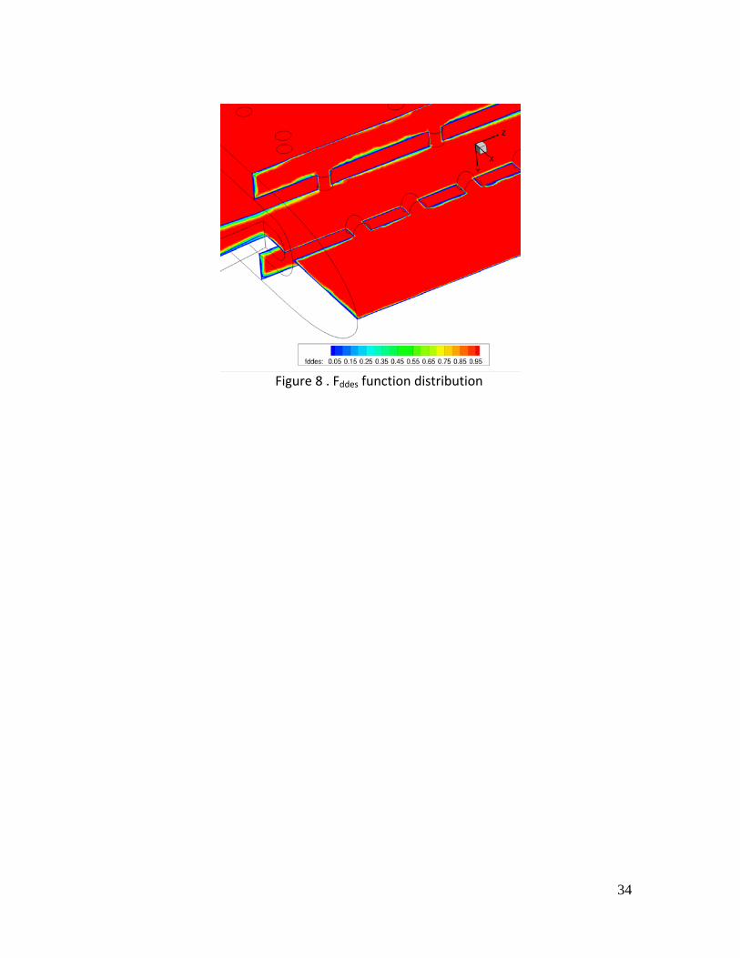
An instantaneous distribution of the unsteady obtained solution can be seen in

Figure 7. The flow is fully turbulent with large scale vortices and a hole dependent

pattern. Concerning the hybrid ZDES treatment, the distinction between the URANS and

the LES treated zones can be seen using the fddes function. When this function is close to

0, the zone is treated in a RANS mode, whereas when close to 1, the simulation is in a

LES mode. Figure 8 confirms that the URANS treatment is applied to near-wall zones,

whereas all other zones are resolved on a LES basis, which explains the fully unsteady

behavior captured in Figure 7. For simplicity reasons, only time-averaged results will be

presented from now on.

AERODYNAMIC RESULTS

Throughout this document, the coordinates (X, Y, Z) denote respectively the

Cartesian coordinates as presented in Figure 3. The axis originates at the exit of the

central hole on the leading edge (fifth hole of row1), on its axis. The fluid flow will be

presented comparing experimental measurements to their numerical counterparts,

being either RANS or ZDES results. The topology of the flow is not considerably modified

by the RANS model used. The results provided by RANS and ZDES approaches are also

qualitatively similar. On the contrary, the heat transfer level is strongly dependent on

the model. For the RANS simulation, the flow topology will therefore be described based

on the results obtained with the k-ω SST model. The flow topology can be visualized on

Figure 9. The air feeds the central cavity through the lateral inlet. Due to the pressure

difference, this air will go through the different holes and impinge on the opposing

walls. The available mass flow rate diminishes along the central cavity, corresponding to

13

a velocity decrease. The velocity profiles inside the different holes appear to be strongly

heterogeneous as shown in Figure 10. This figure presents mass flow rates measured in

each hole of the leading edge and on the pressure side of the vane. As pressure and

suction sides are geometrically symmetric, their mass flow rate distributions are nearly

identical (consequently, suction side distribution is not presented here). The leading

edge row (row1) is globally better supplied (1.22 time higher than the three other rows

on average) due to the greater injection diameters (D2=1.25 D1). The distribution of the

mass flow rate for each row is globally the same. In particular, lowest mas flow rates are

recorded for Z=80mm for every rows. This is due to a large recirculation zone in the

central cavity near the penultimate hole of the fourth row. This recirculation is due to

the main flow that impinges the central cavity right wall (X=200mm) and is turned to the

back of the cavity.

As a matter of fact, the air comes from the central cavity horizontally and is

strongly deviated to go through the holes. For the leading edge holes, this results in a

concentration of the mass flow rate in the downstream part of the hole as seen on

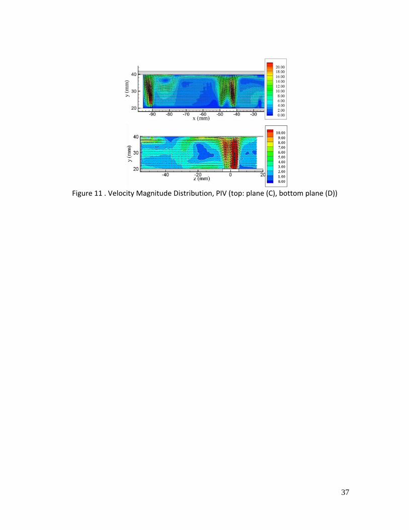
Figure 11-bottom. The upstream part of the perforation is characterized by a

recirculation zone, with low velocity magnitudes. On the pressure side of the vane, the

hole flows are even more complex. For example, Figure 11 presents velocity fields

resulting from PIV measurements of plane (C) and (D) (see Figure 3 for the plane

definition). Those fields show the flow around the third injection of the second row of

injection (on the pressure side). The upper velocity field shows clearly that most of flow

is injected through the side of the injection hole with a small recirculation zone at the

14

center. Moreover, velocity values are higher and the width of the jet is greater for the

low X side of the injection. In the orthogonal plane (lower velocity fields of Figure 11),

flow is injected through the downstream part of the hole (upper Z axis). Consequently,

the injection flow presents a crescent shape with a mass flow rate concentrated over a

quarter of the injection hole (lower X, upper Z axis). Those characteristics of the flow

differ from the fully developed profiles considered in single jet studies and mostly often

adopted for code validation. The strong acceleration and turning of the flow at the hole

inlet also correspond to a far from equilibrium situation from a turbulent point of view,

and one can expect a bad prediction of the turbulent profiles in that region. On Figure

12, which represents RMS velocity fields, we can notice some major differences

between jets on pressure side and more academic jets (issuing from a long tube or a

contraction nozzle): in plane C the highest levels of turbulence are not recorded in the

shear layer but in the jet. Moreover, RMS values tend to be lower away from the

injection which is exactly the opposite of an academic jet.

For the leading edge, the comparison between PIV acquisitions and CEDRE

results is showed in Figure 13 and Figure 14. The location of the slice is detailed in Figure

3. The analysis of Figure 13 reveals a minimum velocity at the hole center, and a

maximum one near the edges of the holes. This result, however surprising it may

appear, is explained by the strong deviation of the flow at the hole inlet. This deviation

explains also the increase of mean velocity values in the central part of the jet

(2mm<X<20mm): it is due to the flow injected through the downstream part of the hole

going upstream. For X>20mm, the velocity mean distribution of the jet become similar

15

to an academic jet one even if RMS values visible in Figure 14 (top) are still very

different. Finally, the impinged plate curvature has also consequences on the jet flow, in

particular on the two large recirculations situated on both sides of the jet (lowest

velocity values in Figure 13). The 3D flow is also visible in Figure 15, presenting the

velocity fields in a plane between two injections. The flow is relatively complex with two

contra-rotating recirculation cells located at (X=30mm; Y=-108mm) and (X=40mm;

Y=12mm). Moreover, high velocities along the curved plate show that a large part of the

flow moves along the Z axis. As stated before, the flow velocity is maximum in the

downstream part of the hole and a slice going through the center of the hole will exhibit

high levels of velocity near the walls and a minimum far from the wall, as confirmed by

Figure 16. The analysis of Figure 16 also reveals secondary kidney-shaped vortices inside

the holes, due to the strong deviation of the flow at the hole inlet. Those secondary

vortices will gradually bring the high velocity air of the downstream part of the hole to

the upstream part along the wall. Coming to the comparison on velocity magnitudes,

Figure 13 reveals a good agreement between experiment and calculation. The main

difference appears in the jet penetration, the measured jet being less diffused than the

simulated one. The analysis of the RMS distributions provided in Figure 14 confirms that

the turbulent fluctuations are qualitatively in good agreement with the measurements,

but underestimate the turbulent fluctuations, in particular in the mixing layer regions.

This underestimation of the turbulent fluctuations leads to a lower level of

turbulent mixing at the hole exit, leading to a stronger penetration of the jet in the

simulation. Coming to ZDES results, the agreement between ZDES and experiment is

16

qualitatively and quantitatively good. Compared to RANS modelling the penetration of

the jet is less intense and closer to PIV measurements. This can be traced back to a

better description of the unsteady structures issued from the holes.

Those unsteady structures contain a major part of the turbulent energy that

cannot be represented by RANS modelling. This conclusion is also obtained on RMS

quantities, which exhibit more intense levels, corresponding to higher levels of

turbulent mixing at the exit of the holes

HEAT TRANSFER RESULTS

For experimental results, the heat transfer coefficient and the reference

temperature are evaluated from a linear regression (see Heat transfer measurement

above). Four different flux densities (from 500W/m² to 2000W/m²) are prescribed. The

air temperature injected into the test section is maintained equal to 296K.

Consequently, the reference temperature measured on the impinged plate is nearly

constant and equal to 296K For the RANS modelling, the heat transfer coefficient is

derived from the formula:

where Tref is taken to the inlet total temperature of 296 K.

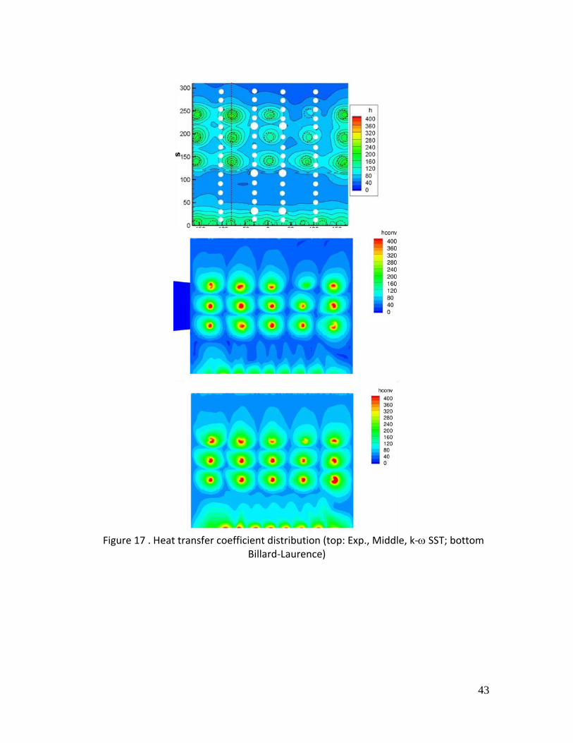
The experimental distribution is showed in Figure 17. Results obtained with the

k−ω SST and Billard Laurence models are also provided. For formatting reasons, the

distributions obtained with the VALM and DRSM models are not presented here. The

experimental heat transfer distribution exhibits local maxima due to the impact of the

17

cooling jets. The maximum value is approximately around 200 W/m2/K in the

impingement regions on the pressure and suction sides, and around 140 W/m2/K in the

leading edge region. The heat transfer distribution also depends on the column

considered and can be directly related to the mass flow rate going through the hole. In

particular, h values in front of the fourth hole of row 4 are clearly lower due to the small

mass flow rate injected (see Figure 8). One noticeable exception is the leading edge

region which presents lower maximum h values than pressure and suction sides with

globally higher mass flow rate injected in the holes. This could be explained by the larger

injection-to-plate distance on the leading edge and by the rapid velocity decrease noted

on Figure 11 (top). Due to the specific injection flow, the jet flow velocity rapidly

decreases causing the drop of heat transfer rate. Another important characteristic of

the leading edge heat transfer rate is its relative homogeneity due to the flow

movement along the Z axis and the relative small jet-to-jet spacing. On the pressure

side, due to the larger jet-to-jet spacing and smaller injection to plate distance,

impinging areas are well defined. It is to be noticed that h maxima are not always

situated in front of their respective injection (represented by black dashed circles) and

their relative position depend on the injection. This is particularly visible for injections

situated on the right side of the impinged plate. This gap between axis injection and h

maxima is the consequence of the non-axisymmetric distribution of the flow in the

holes.

18

Coming to simulations all models strongly overestimate the heat transfer level in

the impingement regions. A maximum value around 400 W/m2/K is predicted by all

models, corresponding to a 100 % discrepancy compared to measured value. However,

the topology of the heat transfer distribution is in qualitative good agreement with the

experimental one in terms of peak location. The lower values obtained at the second

column are also reproduced by the simulation. This fairly good qualitative agreement

can be traced back to a topologically correct prediction of the fluid flow in the cavity.

The poor prediction obtained in terms of heat transfer can probably be attributed to a

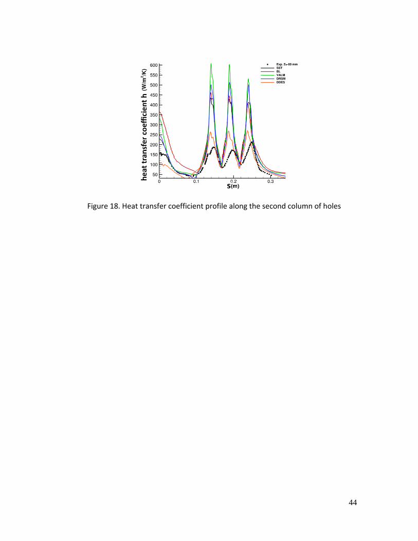
unsatisfactory damping of the turbulence to the wall. The comparison between the

results obtained with the different RANS models can be visualized in Figure 18, where

the heat transfer coefficient profile along the second column of holes is plotted. All

models exhibit the aforementioned overestimation in the pressure/suction side region,

that is for small H/D ratio. The behavior at the leading edge is somewhat different The

Billard-Laurence model offers the poorest prediction with an estimated htc of 350

W/m2/K instead of 150 W/m2/k. The best predictions are brought by the k-ω SST and

DRSM models. Once again the peaks locations, and the overall topology of the htc

distribution are in good agreement with the measured values.

The poor performance of all RANS models is contrary to what is expected based

on a literature survey. In particular, the poor behavior of the Billard-Laurence model is

still to be explained. The most probable explanation relies on the turbulence profiles at

the hole exit, which are from those usually adopted in the single jet configuration. As a

matter of fact, in the single jet configuration, the injected profiles are those of a fully

19

developed channel, with lower turbulent maxima located near the walls. The central

part of the turbulent profile (which is the one influencing the maximum heat transfer

level), corresponds to a fairly low level of turbulent viscosity. The heat transfer obtained

using the ZDES approach can be seen on Figure 18. For comparison purposes, the

experimental and RANS results are presented on the same figure. The heat transfer

levels are in a better agreement with the measured heat transfer. On the pressure and

suction sides, the maxima are around 250 w/m2/K to be compared instead of 200

w/m2/K. This 20% discrepancy has to be compared with the one for RANS models, which

was around 100%. At the leading edge, the heat levels are underestimated by the

simulation by 30%. A possible explanation relies in a mesh still too coarse. The distance

between the holes and the impinging plate being more important at the leading edge,

the numerical dissipation operates on a larger region, leading to an overestimated

dissipation of the turbulent structures at the jet boundaries. As already stated, the mesh

discretization could not be improved due to CPU time constraints, and this hypothesis

could not be checked out.

CONCLUSIONS

The present study investigates the flow field and heat transfer inside a

simplified, however representative, cooling scheme of a turbine vane. Detailed velocity

measurements are obtained through the use of PIV measurements whereas heat

transfer cartographies are detailed using IR acquisitions. The flow topology is complex

with a strongly heterogeneous mass flow rate distribution between the holes, and

noticeable heat transfer maxima in impinging regions. RANS and ZDES simulations were

20

conducted on this configuration. The qualitative agreement between PIV and simulation

is reasonable for fluid flow results, the RANS simulations overestimating the penetration

of the jets in the cooled cavity. The ZDES approach offers a better prediction of the

turbulent mixing of the jets. As a consequence, the prediction of heat transfer is

acceptable with ZDES, whereas a 100% overestimation is obtained with RANS

approaches, even with models showing good agreement with measurement on simpler

configurations.

ACKNOWLEDGMENT The authors acknowledge the financial support of French Direction Generale de

l’Aviation Civile (DGAC) in the framework of Research Programs ARCAE and AETHER.

21

NOMENCLATURE

D1 Jet Diameter of pressure and suction sides holes m

D2 Jet Diameter of leading edge holes (=1.25 D1) m

h Heat transfer coefficient on impinged side of the impinged

plate

Wm-2K-1

X, Y, Z Cartesian coordinates m

Re Injection Reynolds number =ρuD/μ

Tref Adiabatic wall temperature K

Tw Impinging side wall temperature K

u, v, w Mean velocities in the cartesian system ms-1

uRMS,vRMS,wRMS Root mean square velocities in the cylindrical system ms-1

Greek symbols

εw Impinged plate emissivity

λair Air thermal conductivity Wm-1K-1

λw Impinged plate thermal conductivity Wm-1K-1

μ air Air dynamic viscosity Nsm-2

ρair Air density kgm-3

ϕconv Convective heat flux density on the impinged side Wm-2

22

REFERENCES [1] Martin, H., 1977, “Heat and Mass Transfer between Impinging Gas Jets and Solid Surfaces,” Advances in Heat Transfer, vol. 4, pp. 1-60. [2] Jambunathan, K., Lai, E., Moss, M. A. and Button, B. L., 1992, “A review of heat transfer data for single circular jet impingement,” International journal of heat and fluid flow, vol. 13, no. 2, pp. 106-115. [3] Viskanta R., 1993, “Heat transfer to impinging isothermal gas and flame jets,” Experimental thermal and fluid science, vol. 6, no. 2, pp. 111-134. [4] Zuckerman, N. and Lior, N., 2006, “Jet impingement heat transfer:physics, correlations, and numerical modeling,” Advances in Heat Transfer, vol. 39, pp. 565-631. [5] Goldstein, R. and Behbahani, A., 1982,“ Impingement of a circular jet with and without cross flow,” International Journal of Heat Mass Transfer , vol. 25, pp. 1377-1382. [6] Roux, S., Fénot, M., Lalizel, G., Brizzi, L. and Dorignac, E., 2011,“Experimental investigation of the flow and heat transfer of an impinging jet under acoustic excitation,” International Journal of Heat and Mass Transfer, vol. 54, no. 15-16, pp. 3277-3290, 2011. [7] Baughn, J. and Shimizu, S., 1989,“Heat transfer measurements from a surface with uniform heat flux and an impinging jet,” Journal of Heat Transfer, vol. 111, no. 4, pp. 1096-1098. [8] Weigand, B., and Spring, S., 2011, “Multiple Jet Impingement-A Review,”Heat Transfer Res., 42(2), pp. 101–142.

[9] Florschuetz, L. W., Truman, C. R., and Metzger, D. E., 1981,“Streamwise Flow and Heat Transfer Distributions for Jet Array Impingement with Crossflow,” ASME J. Heat Transfer, 103(2), pp. 337–342. [10] Fenot, M. and Dorignac, E., 2016, “Heat transfer and flow structure of an impinging jet with upstream flow,” International Journal of Thermal Sciences, vol. 109, pp. 386-400. [11] Liu ,T., Sullivan, J.P.,1996, “Heat transfer and flow structures in an excited circular impinging jet,” International Journal of Heat and Mass Transfer, vol. 39, issue 17, pp. 3695-3706.

23

[12] Coleman, H.W., and Steele W. G., 1999, "Experimentation and uncertainty analysis for engineers," Chichester, United Kingdom: Wiley-Interscience. [13] Refloch, A., Courbet, B., Murrone, A., Villedieu, P., Laurent, C., Gilbank, P., Troyes, J., Tessé, L., Chaineray, G., Dargaud, J.B., Quémerais, E. & Vuillot, F., 2011, “CEDRE software,” Aerospace Lab J. n°2, 2011. [14] Menter, F. R., 1994, "Two-Equation Eddy-Viscosity Turbulence Models for Engineering Applications," AIAA Journal, vol. 32, no. 8, pp. 1598-1605. [15] Billard, F., Laurence, D., 2011, “A robust k – ε, v2/k elliptic blending turbulence model applied to near-wall, separated and buoyant flows,” International journal of Heat and Fluid Flow, vol. 33, issue 1, pp 45-58, 2011. [16] Durbin P., 1991, “Near-wall closure modelling without damping functions,” Theor. Comput. Fluid Dyn., vol. 3, issue 1, pp. 1-13. [17] Benhia, M., Parneix, S., Durbin, P.A., 1998, “Prediction of heat transfer in an axisymmetric turbulent jet on a flat plate,” Int. J. Heat Mass Transfer, 41, 1845-1855. [18] Vanpouille, D., Aupoix, B., Laroche, E., 2015, “Development of an explicit algebraic turbulence model for buoyant flows –Part 2: Model development and validation,” International Journal of Heat and Fluid Flow, Vol 53, pp 195-209. [19] Deck, S., 2005, “Zonal-detached-eddy simulation of the flow around a high-lift configuration,” AIAA Journal, vol. 43, No 11, pp 2372-2384. [20] S. Deck, 2012,“Recent Improvements of the Zonal Detached Eddy Simulation (ZDES) formulation, Theoretical and Computational Fluid Dynamics,” vol 26, no. 6, pp 523-550. [21] Spalart, P., Jou, W., Strelets, M., and Allmaras, S.,1997,” Comments on the feasibility of les for wings, and on a hybrid rans/les approach,” 1rst International Conf. on LES/DNS. [22] Spalart, P., Deck, S., Shur, M., Squires, K., Strelets, M.~K., and Travin, A.,2006, “A new version of detached-eddy simulation, resistant to ambiguous grid densities,” Theoretical and computational fluid dynamics, vol 20, pp180-195. [23] Strelets, M., 2001, “Detached eddy simulation of massively separated flows,” AIAA 39 th Aerospace Sciences Meeting and Exhibit, Reno, NV. [24] Arroyo-Callejo, G., Laroche, E., Millan, P., Leglaye, F., and Chedevergne, F., 2016, “Numerical Investigation of Compound Angle Effusion Cooling Using Differential

24

Reynolds Stress Model and Zonal Detached Eddy Simulation Approaches,” J. Turbomach 138(10).

25

Figure Captions List Fig. 1 Experimental apparatus

Fig. 2 Test section

Fig. 3 PIV measurements planes

Fig. 4 Heat transfer determination principle

Fig. 5 Fine mesh overview

Fig. 6 Mesh overview for ZDES modelling

Fig. 7 ZDES Velocity magnitude overview

Fig. 8 Fddes function distribution

Fig. 9 Velocity magnitude in a slice going through row 2 (CEDRE k-ω SST)

Fig. 10 Mass flow rate distribution

Fig. 11 Velocity Magnitude Distribution, PIV (top: plane (C), bottom plane (D))

Fig. 12 Velocity RMS Distribution, PIV (top : plane (C), bottom plane (D))

Fig. 13 Velocity Magnitude Distribution, plane (A) (top : PIV, middle CEDRE

RANS, bottom CEDRE, ZDES )

Fig. 14 Axial velocity RMS Distribution, plane (A) (top : PIV, bottom CEDRE k-ω

SST)

Fig. 15 Velocity Magnitude Distribution , plane (B), PIV

Fig. 16 Velocity Distribution/Streamlines colored by velocity inside the hole

26

Fig. 17 Heat transfer coefficient distribution (top: Exp., Middle, k-ω SST; bottom

Billard-Laurence)

Fig. 18 Heat transfer coefficient profile along the second column of holes

27

Figure 1. Experimental apparatus

28

Figure 2. Test section

29

Figure 3. PIV measurements planes

30

Figure 4. Heat transfer determination principle

31

Figure 5. Fine mesh overview

32

Figure 6 . Mesh overview for ZDES modelling

33

Figure 7 : ZDES Velocity magnitude overview

34

Figure 8 . Fddes function distribution

35

Figure 9 : Velocity magnitude in a slice going through row 2 (CEDRE k-ω SST)

36

Figure 10 . Mass flow rates

37

Figure 11 . Velocity Magnitude Distribution, PIV (top: plane (C), bottom plane (D))

38

Figure 12 . Velocity RMS Distribution, PIV (top : plane (C), bottom plane (D))

39

Figure 13. Velocity Magnitude Distribution, plane (A) (top : PIV, middle CEDRE RANS,

bottom CEDRE, ZDES )

40

Figure 14 . Axial velocity RMS Distribution, plane (A) (top : PIV, bottom CEDRE k-ω SST)

41

Figure 15 . Velocity Magnitude Distribution , plane (B), PIV

42

Figure 16 . Velocity Distribution/Streamlines colored by velocity inside the hole

43

Figure 17 . Heat transfer coefficient distribution (top: Exp., Middle, k-ω SST; bottom

Billard-Laurence)

44

Figure 18. Heat transfer coefficient profile along the second column of holes