A coil magnetic levitation simulator for physics …fusioned.gat.com/levitation_phys_educ_sup.pdfA coil magnetic levitation simulator for physics exploration J. A. Leuer1,3, R. Lee1,

Leuer_levitate_phys_educ_sup (supplemental) Page 1 IOP Physics Education, Leuer 04Jan2012

A coil magnetic levitation simulator for physics exploration

J. A. Leuer1,3, R. Lee1, A. Nagy2 1 General Atomics … 2 PPPL … 3 Retired ([email protected]) E-mail: [email protected] or [email protected]

(Supplemental Information) Supplemental Information: http://fusioned.gat.com/

1. This Document: http://fusioned.gat.com/levitation_phys_educ_sup.pdf 2. Excel Spreadsheet: http://fusioned.gat.com/coil_levitate.xls

Contents: Appendix 0: Coil Levitation Spreadsheet USER GUIDE Appendix A: Coil Levitation Spreadsheet Overview and Some Input Hints Appendix B: Circuit Model of Coil Near a Conducting Plate Appendix C: Coil Resistance Appendix D: Current Penetration Depth Appendix E: Vertical Centroid for Current Flowing in the Conducting Plate Appendix F: Coil Heat-up / Temperature Rise Appendix G: Model Validation Using Superconducting Plate Solution


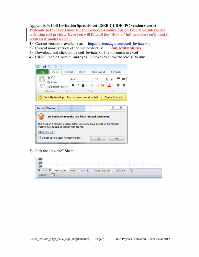
Appendix 0: Coil Levitation Spreadsheet USER GUIDE (PC version shown) Welcome to the User Guide for the General Atomics Fusion Education interactive levitating coil project. Here you will find all the ‘How-to’ information you’ll need to accurately model a coil … 1) Current version is available at: http://fusioned.gat.com/coil_levitate.xls 2) Current name/version of the spreadsheet is: coil_levitate40.xls 3) Download and click on the coil_levitate.xls file to launch in excel 4) Click “Enable Content” and “yes” in boxes to allow “Macro’s” to run:

5) Pick the “levitate” Sheet:


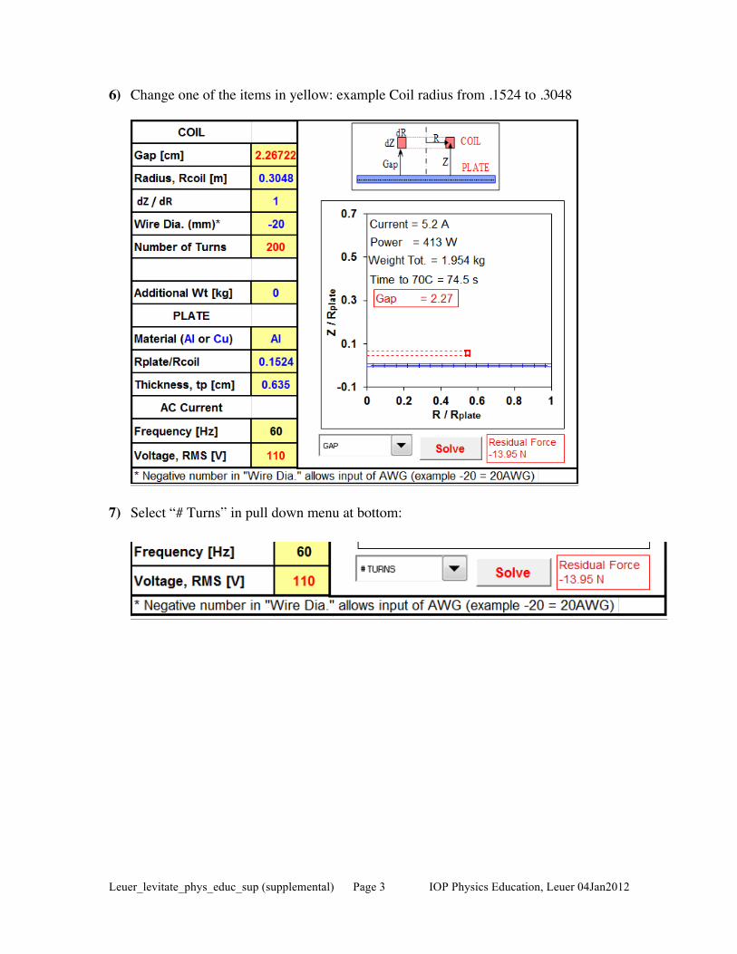
6) Change one of the items in yellow: example Coil radius from .1524 to .3048

7) Select “# Turns” in pull down menu at bottom:


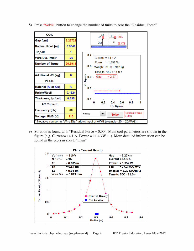
8) Press “Solve” button to change the number of turns to zero the “Residual Force”

9) Solution is found with “Residual Force = 0.00”. Main coil parameters are shown in the figure (e.g. Current= 14.1 A, Power = 11.4 kW …). More detailed information can be found in the plots in sheet: “main”


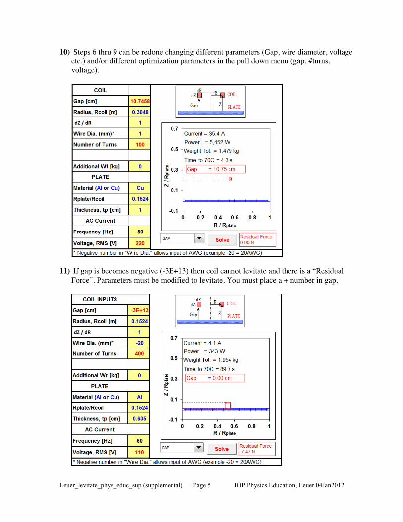
10) Steps 6 thru 9 can be redone changing different parameters (Gap, wire diameter, voltage etc.) and/or different optimization parameters in the pull down menu (gap, #turns, voltage).

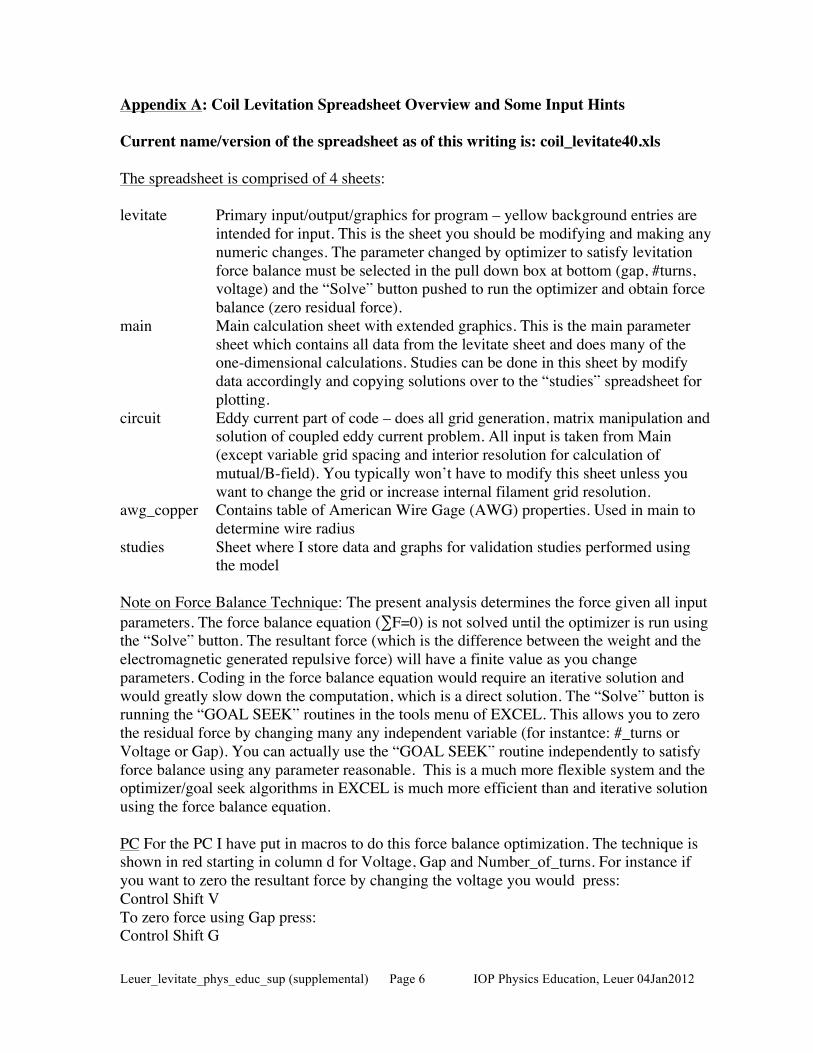
11) If gap is becomes negative (-3E+13) then coil cannot levitate and there is a “Residual

Force”. Parameters must be modified to levitate. You must place a + number in gap.


Appendix A: Coil Levitation Spreadsheet Overview and Some Input Hints Current name/version of the spreadsheet as of this writing is: coil_levitate40.xls The spreadsheet is comprised of 4 sheets: levitate Primary input/output/graphics for program – yellow background entries are

intended for input. This is the sheet you should be modifying and making any numeric changes. The parameter changed by optimizer to satisfy levitation force balance must be selected in the pull down box at bottom (gap, #turns, voltage) and the “Solve” button pushed to run the optimizer and obtain force balance (zero residual force).

main Main calculation sheet with extended graphics. This is the main parameter sheet which contains all data from the levitate sheet and does many of the one-dimensional calculations. Studies can be done in this sheet by modify data accordingly and copying solutions over to the “studies” spreadsheet for plotting.

circuit Eddy current part of code – does all grid generation, matrix manipulation and solution of coupled eddy current problem. All input is taken from Main (except variable grid spacing and interior resolution for calculation of mutual/B-field). You typically won’t have to modify this sheet unless you want to change the grid or increase internal filament grid resolution.

awg_copper Contains table of American Wire Gage (AWG) properties. Used in main to determine wire radius

studies Sheet where I store data and graphs for validation studies performed using the model

Note on Force Balance Technique: The present analysis determines the force given all input parameters. The force balance equation (∑F=0) is not solved until the optimizer is run using the “Solve” button. The resultant force (which is the difference between the weight and the electromagnetic generated repulsive force) will have a finite value as you change parameters. Coding in the force balance equation would require an iterative solution and would greatly slow down the computation, which is a direct solution. The “Solve” button is running the “GOAL SEEK” routines in the tools menu of EXCEL. This allows you to zero the residual force by changing many any independent variable (for instantce: #_turns or Voltage or Gap). You can actually use the “GOAL SEEK” routine independently to satisfy force balance using any parameter reasonable. This is a much more flexible system and the optimizer/goal seek algorithms in EXCEL is much more efficient than and iterative solution using the force balance equation. PC For the PC I have put in macros to do this force balance optimization. The technique is shown in red starting in column d for Voltage, Gap and Number_of_turns. For instance if you want to zero the resultant force by changing the voltage you would press: Control Shift V To zero force using Gap press: Control Shift G


To zero force using Number of turns press: Control Shift N You can also use the manual technique described below in the MAC section: MAC Although the same macros are built into the spreadsheet for the mac or PC, these control_shift_V … macros (which is Options_Command_Shift_V on the mac) do not seem to work properly. The only way zero out the force is to use the “GOAL SEEK” manually. This is done by:

1) Click the mouse on the Resultant Force Cell (Cell D6 Pink). This cell is the dependent variable (force) that we are trying to drive to zero.

2) Open the “Tool” “Goal Seek” Menu. You should see the Cell D6 in the “set cell” box.

3) In the “To Value” box put in 0. This is the value we want the resultant force to become.

4) Click in “By Changing Cell” box and then select cell in workbook to change (i.e. Number of Turns cell D14). Note that the cell you are changing here (D14) can only have a # in it; if a formula is in this cell Excel will complain when you try to solve. This cell is the independent variable Escel will change to drive the force to zero (within a small margin).

5) Press solve and if the problem is well formulated it will arrive at a solution. Press accept or not depending if it got a good solution.

Note that if the solution has problems (perhaps the coil grows so large that its inner radius is on the other side of the axis – not physically possible) you will get “VALUES” for solutions. You must un-edit the changes or go back to an old spreadsheet. Like all numerical algorithms if it finds an discontinuity or some problem equation it will not converge and can contaminate the spreadsheet with “VALUE” numbers. Putting in reasonable numbers typically corrects this but not always. Don't save spreadsheet if this occurs. Stop and re-open a spreadsheet without all the values in the cells and find out what parameters you are putting in which causes an un-real problem (like gap becoming negative or radius becoming negative). If you pose a proper problem the optimizer will always converge. Print Preview: Graphs at the top of the “main” sheet contain most of the important

information. It has been formatted at the bottom of the sheet for use in these plots. The print page area is set to display this region of the spreadsheet and thus you can print preview (or simply print) this page to get a graphical representation of the solution.

Main input parameters are (designated with light yellow background) [example units]: gap Gap between bottom of coil and top of plate surface [m] wire Gauge Wire AWG gauge (like 20 awg). This value is used to select wire radius from

a table on the awg sheet. [20] num. turns Number of turns in the coil [222]


dz Vertical width of the coil. The radial build will be calculated based on the number of turns, extra void fraction and area. Optionally the dz can be computed as 2*rwire so a single turn pancake coil is generated. [m]

Secondary input parameters are (designated with light yellow background) [example units]: fill factor mul. Multiplier to add volume to coil for insulation etc. The coil radial build is

increased to insure the total coil area is equal to the packed wire volume times this “fill factor multiplier”. [1.1 = 10% increase]

Temp(C) Initial temperature of Copper. (30C) Resistiv. @20 This is the resistivity of copper at 20 degrees. Provisions are included to

increase the resistance based on initial temperature (however the heat up resistance for thermal analysis is not yet hooked up)

Frequency Frequency of input voltage power source [60 Hz] Voltage Peak voltage from power source [=110*sqrt(2) = 156 V]. Note: the input cell

for this is up at the top. The cell down in the Coil Voltage Source area (D54) is background colored green and was the normal input for this but is now connected to the cell at top (D7) for ease of goal seeking.

mass mult. Mass multiplier to add weight to coil by multiplying copper weight by this term [1.1 = 10% increased weight due to added insulation etc.]

mass adder mass to add to coil [ 0 kg]. Formula for total mass levitated is: Total coil mass = Cu_mass*mass_multiplyer + mass_add

sheet Resist. This is the sheet resistivity of aluminum. It can change depending on which alloy of Al us use: Pure Al 2.66e-8, Al2024T6 = 4.5e-8, Al6064 = 4.0e-8, (or if you have a copper sheet use: Pure Cu= 1.74e-8

sheet_radius_ratio*(coil_outer_radius). It is meant to put the sheet radius far enough out for the solution not to be sensitive to this parameter. Typical numbers are 1.5 to 2.5. Radius of the sheet must be sufficient so it looks infinite to the coil. However, if it is to large, much of the grid used in the circuit spreadsheet is not utilized. Adjust this parameter to insure the current density plot looks reasonable. When correct, small variations it will have little influence on the solution.

Circuit Resolution input parameters [“circuit sheet”]: Typically all inputs in the “circuit” sheet are derived from the main sheet. However the relative radial grid (which is uniform at present) for the eddy currents can be modified. It is contained in line 5. In addition, a sub grid used to place the filaments within the conductor region is available which can improve the accuracy. The current settings for these are probably adequate for most problems. However, the user can modify these and they should have little impact on the problem if the resolution is high enough. This is especially important for the superconducting validation work where the current flows essentially on the plate surface. Close proximity of filaments can cause inaccuracies. These number are contained in rows 29 & 20 for each circuit for the nr and nz spacing. The 1st set in column I is for the coil and all others are for the eddy current circuits.


Some Techniques and Cautions:

1) This spreadsheet does some pretty sophisticated numerical number crunching. In particular, many Visual Basic routines are included which do much of the complex math. In particular, the elliptic integrals and matrix inversion, multiplication etc are all contained in visual basic routines. Many cells in the circuit are matrix and vector cells which are unlike normal excel cells. You should use caution in modifying stuff in the “circuit” sheet are unless you know what you are doing.

2) Important things on the “main” sheet used in the goal seek have been redefined at the top of the column D. A cell with green background is normally input but it has been connected to input at the of the spreadsheet so it is easy to point to for the “GOAL SEEK” requirement needed to zero the force.

3) Many comments and other useful data are stored to the left of the main column containing the primary data (i.e. Column E,F…). These are meant to be pasted into the primary number column Column D if needed.

4) In the “main” sheet several solutions are presented which are not directly associated with the eddy current problem. The coil-at-infinity problem is done to determine coil currents for a coil not next to a conducting plate.

5) The superconducting-mirror-coil solution is included on the “main” sheet and is for use in validation of the eddy current model. The difference between the current of the superconducting solution and the eddy current model should approach each other if you decrease the aluminum resistivity by several orders of magnitude. This check should be performs routinely to insure that the aluminum plate grid is sufficient to resolve the problem. Cell D99 compares these solutions.

6) The spreadsheet is reasonably general and can easily be modified to do other axisymmetric eddy current problems. In particular, it would be easy to calculate levitation of a sphere between oppositely energized Helmholtz pair of coils. If I get a chance I will set this up.

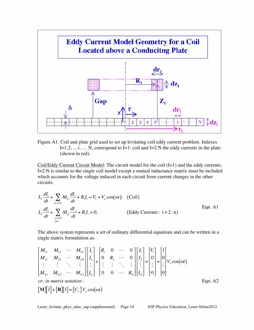
7) Enjoy the model as I did in making it. Jim Leuer, 6/7/2004 Appendix B: Circuit Model of Coil Near a Conducting Plate Eddy Current Geometry: The model formulation follows that in the main text for a coil-at-infinity problem. The only difference is that additional circuits must be added for the currents induced in the plate by the oscillatory currents in the coil. Figure A1 shows the coil and grid used in the plate for the eddy currents. The coil is designated with index I = 1 in the model and the other currents flowing in the plate are designated with index: I = 2,3, … i, … N (red in the figure). N is the total number of conductors in the problem. The location of these additional conductors is at Z= 0 and R= ri and the conductors cross section have dimensions dz and dri. These conductors are considered single turn conductors with resistivity of aluminum.


Figure A1. Coil and plate grid used to set up levitating coil eddy current problem. Indexes

I=1,2, ... i, … N, correspond to I=1: coil and I=2:N the eddy currents in the plate (shown in red).

Coil/Eddy Current Circuit Model: The circuit model for the coil (I=1) and the eddy currents, I=2:N is similar to the single coil model except a mutual inductance matrix must be included which accounts for the voltage induced in each circuit from current changes in the other circuits:

!

L1dI1dt

+ M1idIidti= 2:N

" + R1I1 =V1 =Vo cos #t( ); {Coil}

LidIidt

+ Mij

dI jdtj=1:N

j$ i

" + RiIi = 0; {Eddy Currents : i = 2 : n} Eqn. A1

The above system represents a set of ordinary differential equations and can be written in a single matrix formulation as:

!

M11 M12 ! M1N

M21 M22 ! M2N

" " # "MN1 MN 2 ! MN 2

"

#

$ $ $ $

%

&

' ' ' '

˙ I 1˙ I 2"˙ I N

"

#

$ $ $ $

%

&

' ' ' '

+

R1 0 ! 00 R2 ! 0" " # "0 0 ! RN

"

#

$ $ $ $

%

&

' ' ' '

I1

I2

"IN

"

#

$ $ $ $

%

&

' ' ' '

=

V1

0"0

"

#

$ $ $ $

%

&

' ' ' '

=

10"0

"

#

$ $ $ $

%

&

' ' ' '

Vo cos (t( )

or, in matrix notation :

M[ ] ˙ I [ ] + R[ ] I[ ] = Cv[ ] Vo cos (t( )

Eqn. A2


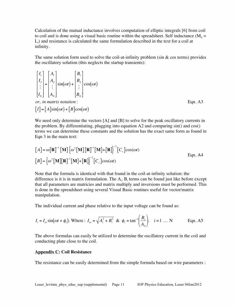
Calculation of the mutual inductance involves computation of elliptic integrals [6] from coil to coil and is done using a visual basic routine within the spreadsheet. Self inductance (Mii = Li) and resistance is calculated the same formulation described in the text for a coil at infinity. The same solution form used to solve the coil-at-infinity problem (sin & cos terms) provides the oscillatory solution (this neglects the startup transients):

!

I1I2!IN

"

#

$ $ $ $

%

&

' ' ' '

=

A1A2

!AN

"

#

$ $ $ $

%

&

' ' ' '

sin (t( ) +

B1B2

!BN

"

#

$ $ $ $

%

&

' ' ' '

cos (t( )

or, in matrix notation :I[ ] = A[ ]sin (t( ) + B[ ]cos (t( )

Eqn. A3

We need only determine the vectors [A] and [B] to solve for the peak oscillatory currents in the problem. By differentiating, plugging into equation A2 and comparing sin() and cos() terms we can determine these constants and the solution has the exact same form as found in Eqn 3 in the main text:

!

A[ ] =" R[ ]#1 M[ ] " 2 M[ ] R[ ]#1 M[ ]+ R[ ]{ }#1Cv[ ]cos("t)

B[ ] = " 2 M[ ] R[ ]#1 M[ ]+ R[ ]{ }#1Cv[ ]cos("t)

Eqn. A4

Note that the formula is identical with that found in the coil-at-infinity solution; the difference is it is in matrix formulation. The Ai, Bi terms can be found just like before except that all parameters are matricies and matrix multiply and inversions must be performed. This is done in the spreadsheet using several Visual Basic routines useful for vector/matrix manipulation. The individual current and phase relative to the input voltage can be found as:

!

Ii = Iio sin "t + #1( ); Where : Iio = Ai2 + Bi

2 & #i = tan$1 Bi

Ai1

%

& '

(

) * ; i =1 … N Eqn. A5

The above formulas can easily be utilized to determine the oscillatory current in the coil and conducting plate close to the coil. Appendix C: Coil Resistance The resistance can be easily determined from the simple formula based on wire parameters :


!

R1 ="cu *LwireAwire

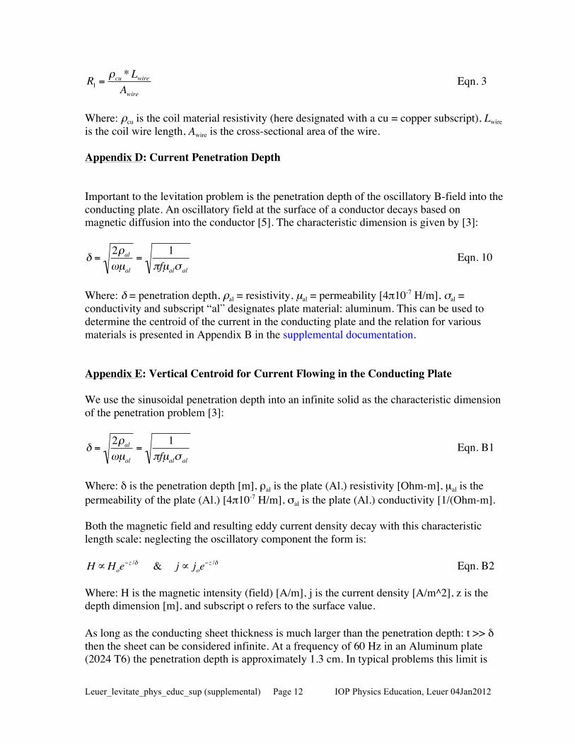
Eqn. 3

Where: ρcu is the coil material resistivity (here designated with a cu = copper subscript), Lwire is the coil wire length, Awire is the cross-sectional area of the wire. Appendix D: Current Penetration Depth Important to the levitation problem is the penetration depth of the oscillatory B-field into the conducting plate. An oscillatory field at the surface of a conductor decays based on magnetic diffusion into the conductor [5]. The characteristic dimension is given by [3]:

!

" =2#al$µal

=1

%fµal& al

Eqn. 10

Where: δ = penetration depth, ρal = resistivity, µal = permeability [4π10-7 H/m], σal = conductivity and subscript “al” designates plate material: aluminum. This can be used to determine the centroid of the current in the conducting plate and the relation for various materials is presented in Appendix B in the supplemental documentation. Appendix E: Vertical Centroid for Current Flowing in the Conducting Plate We use the sinusoidal penetration depth into an infinite solid as the characteristic dimension of the penetration problem [3]:

!

" =2#al$µal

=1

%fµal& al

Eqn. B1

Where: δ is the penetration depth [m], ρal is the plate (Al.) resistivity [Ohm-m], µal is the permeability of the plate (Al.) [4π10-7 H/m], σal is the plate (Al.) conductivity [1/(Ohm-m]. Both the magnetic field and resulting eddy current density decay with this characteristic length scale; neglecting the oscillatory component the form is:

!

H "Hoe#z /$ & j " joe

#z /$ Eqn. B2 Where: H is the magnetic intensity (field) [A/m], j is the current density [A/m^2], z is the depth dimension [m], and subscript o refers to the surface value. As long as the conducting sheet thickness is much larger than the penetration depth: t >> δ then the sheet can be considered infinite. At a frequency of 60 Hz in an Aluminum plate (2024 T6) the penetration depth is approximately 1.3 cm. In typical problems this limit is


only approximately realized. More complex penetration formulation is possible using finite thickness plate [4] but the above simplification should be sufficient to generate reasonably accurate results. We want to determine the centroid of the current for use in our model:

!

" j =zjdz#jdz#

=jo ze$z /" dz#jo e$z /" dz#

= "1$ e$ t /" 1+ t /"( )

1$ e$t /"%

& '

(

) * Eqn. B3

This is the vertical location of the current centroid of the eddy currents relative to the top of the plate. As a check we would expect that δj → 0 as resistivity, ρ → 0, and indeed the above formula in the limit as ρ & δ → 0 then δj → 0. In the other extreme, as δ → ∞ the above formula gives δj → t/2, which corresponds to results for a uniform current distribution in the vertical location. Both extremes seem reasonable. The above formula is used in the spreadsheet for calculation of the current centroid relative to the top of the plate. The gap and coil half height (dz1/2) to determine the vertical distance between coil and plate current centroids. Appendix F: Coil Heat-up / Temperature Rise Excessive coil temperatures are a severe limitation to long-term operation of the coil. Resistive heat input to the conductor (I2 R) is inetrially absorbed by the copper and little of this energy is convected away to the surrounding air unless the coil is brought to an un-acceptably high temperature. We calculate the temperature rise assuming all the resistive energy is absorbed into the copper. The thermal energy equation on a per unit volume basis is:

!

"densityCpdTdt

=Power

V olume

=IrmsVrms

Nturn2#R c Aconductor

Eqn. 11

Where: ρdensity = copper density [8940 kg/m2], Cp = heat capacity [385 J/(kg K)], T = temperature [K],

!

R c = average coil radius, Aconductor= area of conductor = π

!

awire2 [m2] and time

averaged (rms) current (I) and voltage (V) are used. Integration of the above equation provides an estimate of the temperature rise of the coil. In the spreadsheet, additional provisions are provided for including the change in resistivity of the copper as the coil heats-up. The maximum allowable temperature limits the time that the coil can be energized, “coil-on-time”. Appendix G: Model Validation Using Superconducting Plate Solution Here we compare the model against analytical limits expected for a superconducting plate. A simple check of the model can be made by observing that, as the plate conductivity increases, the B-field penetration into the plate decreases and the solution approaches that of a “coil levitated above a superconducting plate”. This can be modeled using a 2nd mirror coil located below the plate surface with the same spacing as the nominal coil to plate surface dimension. Essentially, the mirror coil produces a symmetry plane at the surface of the plate, which is representative of a superconducting plate. Forces can be calculated simply by


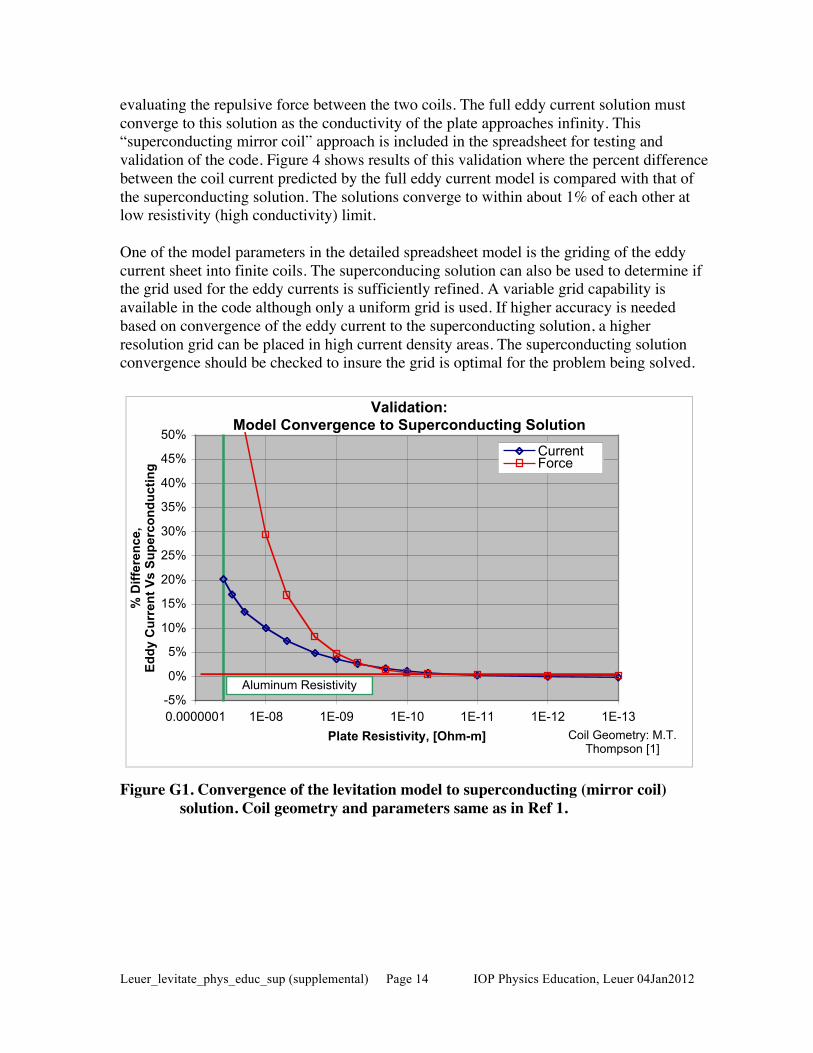
evaluating the repulsive force between the two coils. The full eddy current solution must converge to this solution as the conductivity of the plate approaches infinity. This “superconducting mirror coil” approach is included in the spreadsheet for testing and validation of the code. Figure 4 shows results of this validation where the percent difference between the coil current predicted by the full eddy current model is compared with that of the superconducting solution. The solutions converge to within about 1% of each other at low resistivity (high conductivity) limit. One of the model parameters in the detailed spreadsheet model is the griding of the eddy current sheet into finite coils. The superconducing solution can also be used to determine if the grid used for the eddy currents is sufficiently refined. A variable grid capability is available in the code although only a uniform grid is used. If higher accuracy is needed based on convergence of the eddy current to the superconducting solution, a higher resolution grid can be placed in high current density areas. The superconducting solution convergence should be checked to insure the grid is optimal for the problem being solved.

Validation:Model Convergence to Superconducting Solution

-5%

0%

5%

10%

15%

20%

25%

30%

35%

40%

45%

50%

1E-131E-121E-111E-101E-091E-080.0000001Plate Resistivity, [Ohm-m]

% D

iffer

ence

,Ed

dy C

urre

nt V

s Su

perc

ondu

ctin

g

CurrentForce

Coil Geometry: M.T. Thompson [1]

Aluminum Resistivity

Figure G1. Convergence of the levitation model to superconducting (mirror coil)

solution. Coil geometry and parameters same as in Ref 1.

Documents

A coil magnetic levitation simulator for physics …fusioned.gat.com/levitation_phys_educ_sup.pdfA coil magnetic levitation simulator for physics exploration J. A. Leuer1,3, R. Lee1,