A Closer Look at Memorization in Deep Networks

Devansh Arpit * 1 2 Stanisław Jastrzebski * 3 Nicolas Ballas * 1 2 David Krueger * 1 2 Emmanuel Bengio 4

Maxinder S. Kanwal 5 Tegan Maharaj 1 6 Asja Fischer 7 Aaron Courville 1 2 8 Yoshua Bengio 1 2 9

Simon Lacoste-Julien 1 2

Abstract

We examine the role of memorization in deeplearning, drawing connections to capacity, gen-eralization, and adversarial robustness. Whiledeep networks are capable of memorizing noisedata, our results suggest that they tend to pri-oritize learning simple patterns first. In ourexperiments, we expose qualitative differencesin gradient-based optimization of deep neuralnetworks (DNNs) on noise vs. real data. Wealso demonstrate that for appropriately tunedexplicit regularization (e.g., dropout) we candegrade DNN training performance on noisedatasets without compromising generalization onreal data. Our analysis suggests that the notionsof effective capacity which are dataset indepen-dent are unlikely to explain the generalizationperformance of deep networks when trained withgradient based methods because training data it-self plays an important role in determining thedegree of memorization.

1. IntroductionThe traditional view of generalization holds that a modelwith sufficient capacity (e.g. more parameters than trainingexamples) will be able to “memorize” each example, over-fitting the training set and yielding poor generalization tovalidation and test sets (Goodfellow et al., 2016). Yet deepneural networks (DNNs) often achieve excellent gener-alization performance with massively over-parameterizedmodels. This phenomenon is not well-understood.

*Equal contribution 1Montréal Institute for Learning Algo-rithms, Canada 2Université de Montréal, Canada 3JagiellonianUniversity, Krakow, Poland 4McGill University, Canada5University of California, Berkeley, USA 6PolytechniqueMontréal, Canada 7University of Bonn, Bonn, Germany8CIFAR Fellow 9CIFAR Senior Fellow. Correspondence to:<david.krueger@umontreal.ca>.

Proceedings of the 34 th International Conference on MachineLearning, Sydney, Australia, PMLR 70, 2017. Copyright 2017by the author(s).

From a representation learning perspective, the general-ization capabilities of DNNs are believed to stem fromtheir incorporation of good generic priors (see, e.g., Ben-gio et al. (2009)). Lin & Tegmark (2016) further suggestthat the priors of deep learning are well suited to the phys-ical world. But while the priors of deep learning may helpexplain why DNNs learn to efficiently represent complexreal-world functions, they are not restrictive enough to ruleout memorization.

On the contrary, deep nets are known to be universal ap-proximators, capable of representing arbitrarily complexfunctions given sufficient capacity (Cybenko, 1989; Horniket al., 1989). Furthermore, recent work has shown that theexpressiveness of DNNs grows exponentially with depth(Montufar et al., 2014; Poole et al., 2016). These works,however, only examine the representational capacity, thatis, the set of hypotheses a model is capable of expressingvia some value of its parameters.

Because DNN optimization is not well-understood, it is un-clear which of these hypotheses can actually be reached bygradient-based training (Bottou, 1998). In this sense, opti-mization and generalization are entwined in DNNs. To ac-count for this, we formalize a notion of the effective capac-ity (EC) of a learning algorithm A (defined by specifyingboth the model and the training procedure, e.g.,“train theLeNet architecture (LeCun et al., 1998) for 100 epochs us-ing stochastic gradient descent (SGD) with a learning rateof 0.01”) as the set of hypotheses which can be reachedby applying that learning algorithm on some dataset. For-mally, using set-builder notation:

EC(A) = {h | ∃D such that h ∈ A(D)} ,

where A(D) represents the set of hypotheses that is reach-able by A on a dataset D1.

One might suspect that DNNs effective capacity is suffi-ciently limited by gradient-based training and early stop-ping to resolve the apparent paradox between DNNs’ excel-lent generalization and their high representational capacity.However, the experiments of Zhang et al. (2017) suggestthat this is not the case. They demonstrate that DNNs are

1 Since A can be stochastic, A(D) is a set.

arX

iv:1

706.

0539

4v2

[st

at.M

L]

1 J

ul 2

017

A Closer Look at Memorization in Deep Networks

able to fit pure noise without even needing substantiallylonger training time. Thus even the effective capacity ofDNNs may be too large, from the point of view of tradi-tional learning theory.

By demonstrating the ability of DNNs to “memorize” ran-dom noise, Zhang et al. (2017) also raise the questionwhether deep networks use similar memorization tactics onreal datasets. Intuitively, a brute-force memorization ap-proach to fitting data does not capitalize on patterns sharedbetween training examples or features; the content of whatis memorized is irrelevant. A paradigmatic example ofa memorization algorithm is k-nearest neighbors (Fix &Hodges Jr, 1951). Like Zhang et al. (2017), we do notformally define memorization; rather, we investigate thisintuitive notion of memorization by training DNNs to fitrandom data.

Main Contributions

We operationalize the definition of “memorization” as thebehavior exhibited by DNNs trained on noise, and conducta series of experiments that contrast the learning dynamicsof DNNs on real vs. noise data. Thus, our analysis buildson the work of Zhang et al. (2017) and further investigatesthe role of memorization in DNNs.

Our findings are summarized as follows:

1. There are qualitative differences in DNN optimizationbehavior on real data vs. noise. In other words, DNNsdo not just memorize real data (Section 3).

2. DNNs learn simple patterns first, before memorizing(Section 4). In other words, DNN optimization iscontent-aware, taking advantage of patterns shared bymultiple training examples.

3. Regularization techniques can differentially hindermemorization in DNNs while preserving their abilityto learn about real data (Section 5).

2. Experiment DetailsWe perform experiments on MNIST (LeCun et al., 1998)and CIFAR10 (Krizhevsky et al.) datasets. We investi-gate two classes of models: 2-layer multi-layer percep-trons (MLPs) with rectifier linear units (ReLUs) on MNISTand convolutional neural networks (CNNs) on CIFAR10.If not stated otherwise, the MLPs have 4096 hidden unitsper layer and are trained for 1000 epochs with SGD andlearning rate 0.01. The CNNs are a small Alexnet-styleCNN2 (as in Zhang et al. (2017)), and are trained using

2Input → Crop(2,2) → Conv(200,5,5) → BN → ReLU →MaxPooling(3,3) → Conv(200,5,5) → BN→ ReLU→ MaxPool-

SGD with momentum=0.9 and learning rate of 0.01, sched-uled to drop by half every 15 epochs.

Following Zhang et al. (2017), in many of our experimentswe replace either (some portion of) the labels (with randomlabels), or the inputs (with i.i.d. Gaussian noise matchingthe real dataset’s mean and variance) for some fraction ofthe training set. We use randX and randY to denote datasetswith (100%, unless specified) noisy inputs and labels (re-spectively).

3. Qualitative Differences of DNNs Trainedon Random vs. Real Data

Zhang et al. (2017) empirically demonstrated that DNNsare capable of fitting random data, which implicitly neces-sitates some high degree of memorization. In this section,we investigate whether DNNs employ similar memoriza-tion strategy when trained on real data. In particular, ourexperiments highlight some qualitative differences betweenDNNs trained on real data vs. random data, supporting thefact that DNNs do not use brute-force memorization to fitreal datasets.

3.1. Easy Examples as Evidence of Patterns in RealData

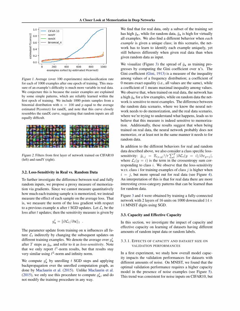
A brute-force memorization approach to fitting data shouldapply equally well to different training examples. How-ever, if a network is learning based on patterns in the data,some examples may fit these patterns better than others. Weshow that such “easy examples” (as well as correspond-ingly “hard examples”) are common in real, but not inrandom, datasets. Specifically, for each setting (real data,randX, randY), we train an MLP for a single epoch start-ing from 100 different random initializations and shufflingsof the data. We find that, for real data, many examplesare consistently classified (in)correctly after a single epoch,suggesting that different examples are significantly easieror harder in this sense. For noise data, the difference be-tween examples is much less, indicating that these exam-ples are fit (more) independently. Results are presented inFigure 1.

For randX, apparent differences in difficulty are well mod-eled as random Binomial noise. For randY, this is not thecase, indicating some use of shared patterns. Visualizingfirst-level features learned by a CNN supports this hypoth-esis (Figure 2).

ing(3,3) → Dense(384) → BN → ReLU → Dense(192) → BN→ ReLU → Dense(#classes) → Softmax. Here Crop(. , .) cropsheight and width from both sides with respective values.

A Closer Look at Memorization in Deep Networks

Figure 1. Average (over 100 experiments) misclassification ratefor each of 1000 examples after one epoch of training. This mea-sure of an example’s difficulty is much more variable in real data.We conjecture this is because the easier examples are explainedby some simple patterns, which are reliably learned within thefirst epoch of training. We include 1000 points samples from abinomial distribution with n = 100 and p equal to the averageestimated P(correct) for randX, and note that this curve closelyresembles the randX curve, suggesting that random inputs are allequally difficult.

Figure 2. Filters from first layer of network trained on CIFAR10(left) and randY (right).

3.2. Loss-Sensitivity in Real vs. Random Data

To further investigate the difference between real and fullyrandom inputs, we propose a proxy measure of memoriza-tion via gradients. Since we cannot measure quantitativelyhow much each training sample x is memorized, we insteadmeasure the effect of each sample on the average loss. Thatis, we measure the norm of the loss gradient with respectto a previous example x after t SGD updates. Let Lt be theloss after t updates; then the sensitivity measure is given by

gtx = ‖∂Lt/∂x‖1 .

The parameter update from training on x influences all fu-ture Lt indirectly by changing the subsequent updates ondifferent training examples. We denote the average over gtxafter T steps as gx, and refer to it as loss-sensitivity. Notethat we only report `1-norm results, but that results stayvery similar using `2-norm and infinity norm.

We compute gtx by unrolling t SGD steps and applyingbackpropagation over the unrolled computation graph, asdone by Maclaurin et al. (2015). Unlike Maclaurin et al.(2015), we only use this procedure to compute gtx, and donot modify the training procedure in any way.

We find that for real data, only a subset of the training sethas high gx, while for random data, gx is high for virtuallyall examples. We also find a different behavior when eachexample is given a unique class; in this scenario, the net-work has to learn to identify each example uniquely, yetstill behaves differently when given real data than whengiven random data as input.

We visualize (Figure 3) the spread of gx as training pro-gresses by computing the Gini coefficient over x’s. TheGini coefficient (Gini, 1913) is a measure of the inequalityamong values of a frequency distribution; a coefficient of0 means exact equality (i.e., all values are the same), whilea coefficient of 1 means maximal inequality among values.We observe that, when trained on real data, the network hasa high gx for a few examples, while on random data the net-work is sensitive to most examples. The difference betweenthe random data scenario, where we know the neural net-work needs to do memorization, and the real data scenario,where we’re trying to understand what happens, leads us tobelieve that this measure is indeed sensitive to memoriza-tion. Additionally, these results suggest that when beingtrained on real data, the neural network probably does notmemorize, or at least not in the same manner it needs to forrandom data.

In addition to the different behaviors for real and randomdata described above, we also consider a class specific loss-sensitivity: gi,j = E(x,y)

1/T∑T

t |∂Lt(y = i)/∂xy=j |,where Lt(y = i) is the term in the crossentropy sum cor-responding to class i. We observe that the loss-sensitivityw.r.t. class i for training examples of class j is higher wheni = j, but more spread out for real data (see Figure 4).An interpretation of this is that for real data there are moreinteresting cross-category patterns that can be learned thanfor random data.

Figure 3 and 4 were obtained by training a fully-connectednetwork with 2 layers of 16 units on 1000 downscaled 14×14 MNIST digits using SGD.

3.3. Capacity and Effective Capacity

In this section, we investigate the impact of capacity andeffective capacity on learning of datasets having differentamounts of random input data or random labels.

3.3.1. EFFECTS OF CAPACITY AND DATASET SIZE ONVALIDATION PERFORMANCES

In a first experiment, we study how overall model capac-ity impacts the validation performances for datasets withdifferent amounts of noise. On MNIST, we found that theoptimal validation performance requires a higher capacitymodel in the presence of noise examples (see Figure 5).This trend was consistent for noise inputs on CIFAR10, but

A Closer Look at Memorization in Deep Networks

103 104 105

number of SGD steps (log scale)

0.1

0.2

0.3

0.4

0.5

0.6

0.7

Gin

icoe

fficie

ntofg x

dist

ribut

ion real data

50% real datarandom data

103 104

number of SGD steps (log scale)

0.16

0.18

0.20

0.22

0.24

Gin

icoe

fficie

ntofg x

dist

ribut

ion real data

random data

Figure 3. Plots of the Gini coefficient of gx over examples x (see section 3.2) as training progresses, for a 1000-example real dataset(14x14 MNIST) versus random data. On the left, Y is the normal class label; on the right, there are as many classes as examples, thenetwork has to learn to map each example to a unique class.

0 2 4 6 80

2

4

6

8

0 2 4 6 80

2

4

6

810−7

10−6

Figure 4. Plots of per-class gx (see previous figure; log scale), acell i, j represents the average |∂L(y = i)/∂xy=j |, i.e. the loss-sensitivity of examples of class i w.r.t. training examples of classj. Left is real data, right is random data.

we did not notice any relationship between capacity andvalidation performance on random labels on CIFAR10.

This result contradicts the intuitions of traditional learningtheory, which suggest that capacity should be restricted, inorder to enforce the learning of (only) the most regular pat-terns. Given that DNNs can perfectly fit the training set inany case, we hypothesize that that higher capacity allowsthe network to fit the noise examples in a way that doesnot interfere with learning the real data. In contrast, if wewere simply to remove noise examples, yielding a smaller(clean) dataset, a lower capacity model would be able toachieve optimal performance.

3.3.2. EFFECTS OF CAPACITY AND DATASET SIZE ONTRAINING TIME

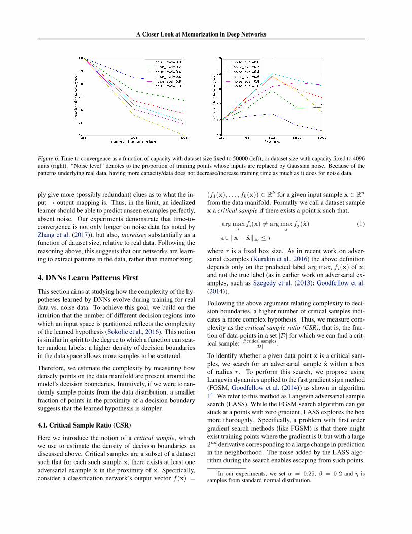
Our next experiment measures time-to-convergence, i.e.how many epochs it takes to reach 100% training accu-racy. Reducing the capacity or increasing the size of thedataset slows down training as well for real as for noise

Figure 5. Performance as a function of capacity in 2-layer MLPstrained on (noisy versions of) MNIST. For real data, performanceis already very close to maximal with 4096 hidden units, but whenthere is noise in the dataset, higher capacity is needed.

data3. However, the effect is more severe for datasets con-taining noise, as our experiments in this section show (seeFigure 6).

Effective capacity of a DNN can be increased by increas-ing the representational capacity (e.g. adding more hiddenunits) or training for longer. Thus, increasing the num-ber of hidden units decreases the number of training iter-ations needed to fit the data, up to some limit. We ob-serve stronger diminishing returns from increasing repre-sentational capacity for real data, indicating that this limitis lower, and a smaller representational capacity is suffi-cient, for real datasets.

Increasing the number of examples (keeping representa-tional capacity fixed) also increases the time needed tomemorize the training set. In the limit, the representa-tional capacity is simply insufficient, and memorization isnot feasible. On the other hand, when the relationship be-tween inputs and outputs is meaningful, new examples sim-

3 Regularization can also increase time-to-convergence; seesection 5.

A Closer Look at Memorization in Deep Networks

Figure 6. Time to convergence as a function of capacity with dataset size fixed to 50000 (left), or dataset size with capacity fixed to 4096units (right). “Noise level” denotes to the proportion of training points whose inputs are replaced by Gaussian noise. Because of thepatterns underlying real data, having more capacity/data does not decrease/increase training time as much as it does for noise data.

ply give more (possibly redundant) clues as to what the in-put → output mapping is. Thus, in the limit, an idealizedlearner should be able to predict unseen examples perfectly,absent noise. Our experiments demonstrate that time-to-convergence is not only longer on noise data (as noted byZhang et al. (2017)), but also, increases substantially as afunction of dataset size, relative to real data. Following thereasoning above, this suggests that our networks are learn-ing to extract patterns in the data, rather than memorizing.

4. DNNs Learn Patterns FirstThis section aims at studying how the complexity of the hy-potheses learned by DNNs evolve during training for realdata vs. noise data. To achieve this goal, we build on theintuition that the number of different decision regions intowhich an input space is partitioned reflects the complexityof the learned hypothesis (Sokolic et al., 2016). This notionis similar in spirit to the degree to which a function can scat-ter random labels: a higher density of decision boundariesin the data space allows more samples to be scattered.

Therefore, we estimate the complexity by measuring howdensely points on the data manifold are present around themodel’s decision boundaries. Intuitively, if we were to ran-domly sample points from the data distribution, a smallerfraction of points in the proximity of a decision boundarysuggests that the learned hypothesis is simpler.

4.1. Critical Sample Ratio (CSR)

Here we introduce the notion of a critical sample, whichwe use to estimate the density of decision boundaries asdiscussed above. Critical samples are a subset of a datasetsuch that for each such sample x, there exists at least oneadversarial example x in the proximity of x. Specifically,consider a classification network’s output vector f(x) =

(f1(x), . . . , fk(x)) ∈ Rk for a given input sample x ∈ Rn

from the data manifold. Formally we call a dataset samplex a critical sample if there exists a point x such that,

arg maxifi(x) 6= arg max

jfj(x) (1)

s.t. ‖x− x‖∞ ≤ r

where r is a fixed box size. As in recent work on adver-sarial examples (Kurakin et al., 2016) the above definitiondepends only on the predicted label arg maxi fi(x) of x,and not the true label (as in earlier work on adversarial ex-amples, such as Szegedy et al. (2013); Goodfellow et al.(2014)).

Following the above argument relating complexity to deci-sion boundaries, a higher number of critical samples indi-cates a more complex hypothesis. Thus, we measure com-plexity as the critical sample ratio (CSR), that is, the frac-tion of data-points in a set |D| for which we can find a crit-ical sample: #critical samples

|D| .

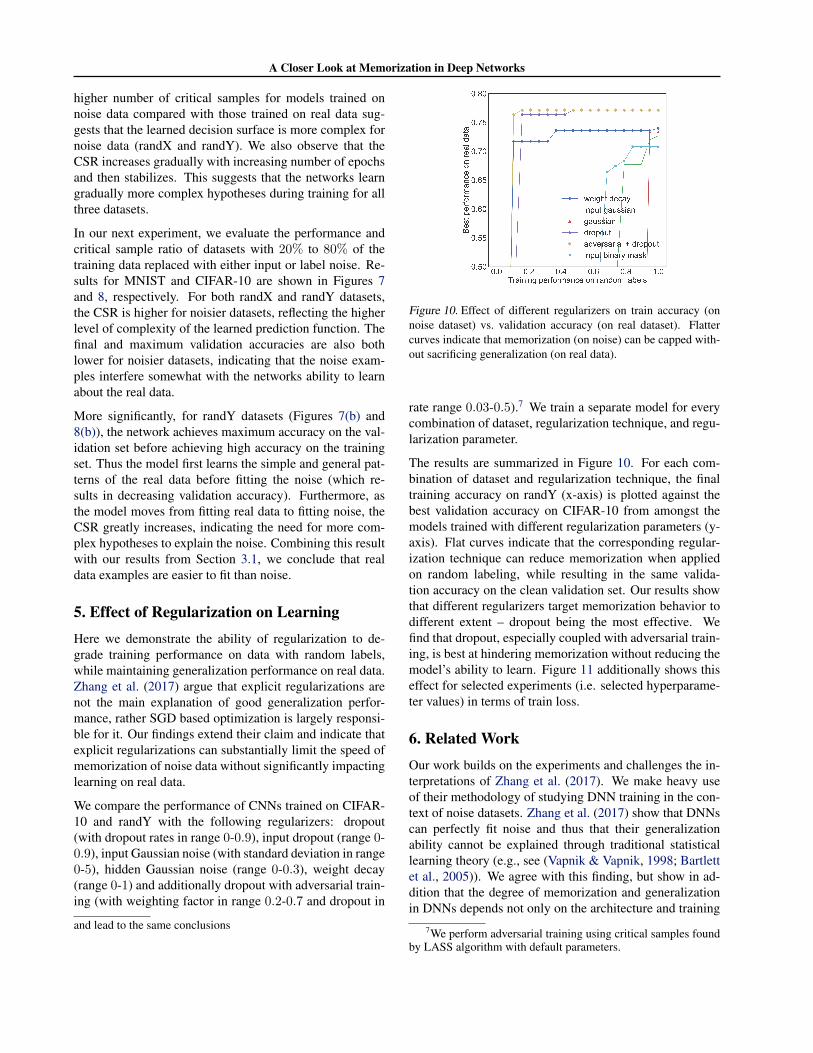
To identify whether a given data point x is a critical sam-ples, we search for an adversarial sample x within a boxof radius r. To perform this search, we propose usingLangevin dynamics applied to the fast gradient sign method(FGSM, Goodfellow et al. (2014)) as shown in algorithm14. We refer to this method as Langevin adversarial samplesearch (LASS). While the FGSM search algorithm can getstuck at a points with zero gradient, LASS explores the boxmore thoroughly. Specifically, a problem with first ordergradient search methods (like FGSM) is that there mightexist training points where the gradient is 0, but with a large2nd derivative corresponding to a large change in predictionin the neighborhood. The noise added by the LASS algo-rithm during the search enables escaping from such points.

4In our experiments, we set α = 0.25, β = 0.2 and η issamples from standard normal distribution.

A Closer Look at Memorization in Deep Networks

(a) Noise added on classification inputs. (b) Noise added on classification labels.

Figure 7. Accuracy (left in each pair, solid is train, dotted is validation) and Critical sample ratios (right in each pair) for MNIST.

(a) Noise added on classification inputs. (b) Noise added on classification labels.

Figure 8. Accuracy (left in each pair, solid is train, dotted is validation) and Critical sample ratios (right in each pair) for CIFAR10.

Algorithm 1 Langevin Adversarial Sample Search (LASS)Require: x ∈ Rn, α, β, r, noise process ηEnsure: x

1: converged = FALSE2: x← x; x← ∅3: while not converged or max iter reached do4: ∆ = α · sign(∂fk(x)

∂x ) + β · η5: x← x + ∆6: for i ∈ [n] do

7: xi ←{

xi + r · sign(xi − xi) if |xi − xi| > rxi otherwise

8: end for9: if arg maxi f(x) 6= arg maxi f(x) then

10: converged = TRUE11: x← x12: end if13: end while

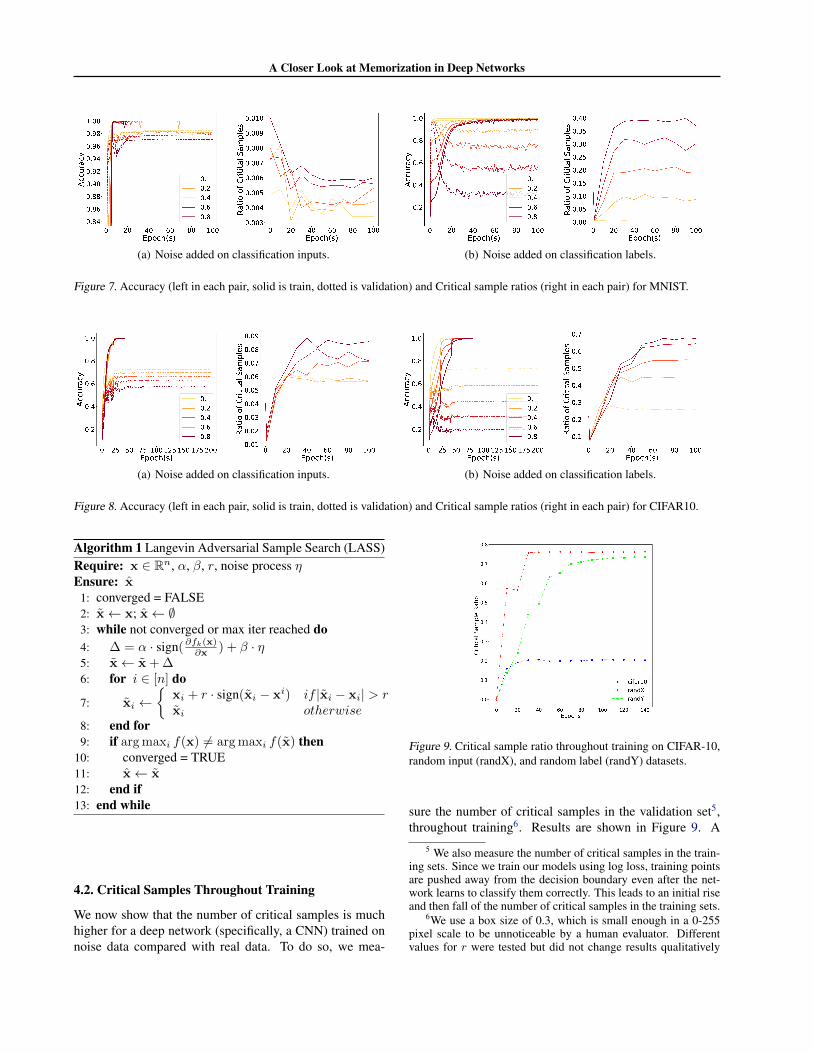
4.2. Critical Samples Throughout Training

We now show that the number of critical samples is muchhigher for a deep network (specifically, a CNN) trained onnoise data compared with real data. To do so, we mea-

Figure 9. Critical sample ratio throughout training on CIFAR-10,random input (randX), and random label (randY) datasets.

sure the number of critical samples in the validation set5,throughout training6. Results are shown in Figure 9. A

5 We also measure the number of critical samples in the train-ing sets. Since we train our models using log loss, training pointsare pushed away from the decision boundary even after the net-work learns to classify them correctly. This leads to an initial riseand then fall of the number of critical samples in the training sets.

6We use a box size of 0.3, which is small enough in a 0-255pixel scale to be unnoticeable by a human evaluator. Differentvalues for r were tested but did not change results qualitatively

A Closer Look at Memorization in Deep Networks

higher number of critical samples for models trained onnoise data compared with those trained on real data sug-gests that the learned decision surface is more complex fornoise data (randX and randY). We also observe that theCSR increases gradually with increasing number of epochsand then stabilizes. This suggests that the networks learngradually more complex hypotheses during training for allthree datasets.

In our next experiment, we evaluate the performance andcritical sample ratio of datasets with 20% to 80% of thetraining data replaced with either input or label noise. Re-sults for MNIST and CIFAR-10 are shown in Figures 7and 8, respectively. For both randX and randY datasets,the CSR is higher for noisier datasets, reflecting the higherlevel of complexity of the learned prediction function. Thefinal and maximum validation accuracies are also bothlower for noisier datasets, indicating that the noise exam-ples interfere somewhat with the networks ability to learnabout the real data.

More significantly, for randY datasets (Figures 7(b) and8(b)), the network achieves maximum accuracy on the val-idation set before achieving high accuracy on the trainingset. Thus the model first learns the simple and general pat-terns of the real data before fitting the noise (which re-sults in decreasing validation accuracy). Furthermore, asthe model moves from fitting real data to fitting noise, theCSR greatly increases, indicating the need for more com-plex hypotheses to explain the noise. Combining this resultwith our results from Section 3.1, we conclude that realdata examples are easier to fit than noise.

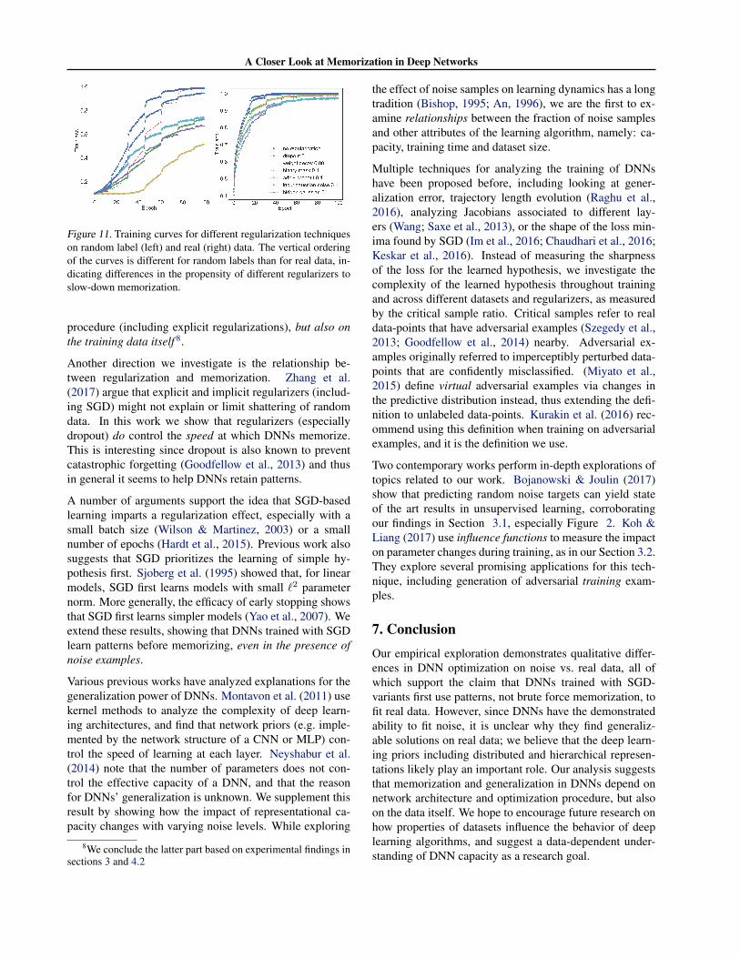
5. Effect of Regularization on LearningHere we demonstrate the ability of regularization to de-grade training performance on data with random labels,while maintaining generalization performance on real data.Zhang et al. (2017) argue that explicit regularizations arenot the main explanation of good generalization perfor-mance, rather SGD based optimization is largely responsi-ble for it. Our findings extend their claim and indicate thatexplicit regularizations can substantially limit the speed ofmemorization of noise data without significantly impactinglearning on real data.

We compare the performance of CNNs trained on CIFAR-10 and randY with the following regularizers: dropout(with dropout rates in range 0-0.9), input dropout (range 0-0.9), input Gaussian noise (with standard deviation in range0-5), hidden Gaussian noise (range 0-0.3), weight decay(range 0-1) and additionally dropout with adversarial train-ing (with weighting factor in range 0.2-0.7 and dropout in

and lead to the same conclusions

Figure 10. Effect of different regularizers on train accuracy (onnoise dataset) vs. validation accuracy (on real dataset). Flattercurves indicate that memorization (on noise) can be capped with-out sacrificing generalization (on real data).

rate range 0.03-0.5).7 We train a separate model for everycombination of dataset, regularization technique, and regu-larization parameter.

The results are summarized in Figure 10. For each com-bination of dataset and regularization technique, the finaltraining accuracy on randY (x-axis) is plotted against thebest validation accuracy on CIFAR-10 from amongst themodels trained with different regularization parameters (y-axis). Flat curves indicate that the corresponding regular-ization technique can reduce memorization when appliedon random labeling, while resulting in the same valida-tion accuracy on the clean validation set. Our results showthat different regularizers target memorization behavior todifferent extent – dropout being the most effective. Wefind that dropout, especially coupled with adversarial train-ing, is best at hindering memorization without reducing themodel’s ability to learn. Figure 11 additionally shows thiseffect for selected experiments (i.e. selected hyperparame-ter values) in terms of train loss.

6. Related WorkOur work builds on the experiments and challenges the in-terpretations of Zhang et al. (2017). We make heavy useof their methodology of studying DNN training in the con-text of noise datasets. Zhang et al. (2017) show that DNNscan perfectly fit noise and thus that their generalizationability cannot be explained through traditional statisticallearning theory (e.g., see (Vapnik & Vapnik, 1998; Bartlettet al., 2005)). We agree with this finding, but show in ad-dition that the degree of memorization and generalizationin DNNs depends not only on the architecture and training

7We perform adversarial training using critical samples foundby LASS algorithm with default parameters.

A Closer Look at Memorization in Deep Networks

Figure 11. Training curves for different regularization techniqueson random label (left) and real (right) data. The vertical orderingof the curves is different for random labels than for real data, in-dicating differences in the propensity of different regularizers toslow-down memorization.

procedure (including explicit regularizations), but also onthe training data itself 8.

Another direction we investigate is the relationship be-tween regularization and memorization. Zhang et al.(2017) argue that explicit and implicit regularizers (includ-ing SGD) might not explain or limit shattering of randomdata. In this work we show that regularizers (especiallydropout) do control the speed at which DNNs memorize.This is interesting since dropout is also known to preventcatastrophic forgetting (Goodfellow et al., 2013) and thusin general it seems to help DNNs retain patterns.

A number of arguments support the idea that SGD-basedlearning imparts a regularization effect, especially with asmall batch size (Wilson & Martinez, 2003) or a smallnumber of epochs (Hardt et al., 2015). Previous work alsosuggests that SGD prioritizes the learning of simple hy-pothesis first. Sjoberg et al. (1995) showed that, for linearmodels, SGD first learns models with small `2 parameternorm. More generally, the efficacy of early stopping showsthat SGD first learns simpler models (Yao et al., 2007). Weextend these results, showing that DNNs trained with SGDlearn patterns before memorizing, even in the presence ofnoise examples.

Various previous works have analyzed explanations for thegeneralization power of DNNs. Montavon et al. (2011) usekernel methods to analyze the complexity of deep learn-ing architectures, and find that network priors (e.g. imple-mented by the network structure of a CNN or MLP) con-trol the speed of learning at each layer. Neyshabur et al.(2014) note that the number of parameters does not con-trol the effective capacity of a DNN, and that the reasonfor DNNs’ generalization is unknown. We supplement thisresult by showing how the impact of representational ca-pacity changes with varying noise levels. While exploring

8We conclude the latter part based on experimental findings insections 3 and 4.2

the effect of noise samples on learning dynamics has a longtradition (Bishop, 1995; An, 1996), we are the first to ex-amine relationships between the fraction of noise samplesand other attributes of the learning algorithm, namely: ca-pacity, training time and dataset size.

Multiple techniques for analyzing the training of DNNshave been proposed before, including looking at gener-alization error, trajectory length evolution (Raghu et al.,2016), analyzing Jacobians associated to different lay-ers (Wang; Saxe et al., 2013), or the shape of the loss min-ima found by SGD (Im et al., 2016; Chaudhari et al., 2016;Keskar et al., 2016). Instead of measuring the sharpnessof the loss for the learned hypothesis, we investigate thecomplexity of the learned hypothesis throughout trainingand across different datasets and regularizers, as measuredby the critical sample ratio. Critical samples refer to realdata-points that have adversarial examples (Szegedy et al.,2013; Goodfellow et al., 2014) nearby. Adversarial ex-amples originally referred to imperceptibly perturbed data-points that are confidently misclassified. (Miyato et al.,2015) define virtual adversarial examples via changes inthe predictive distribution instead, thus extending the defi-nition to unlabeled data-points. Kurakin et al. (2016) rec-ommend using this definition when training on adversarialexamples, and it is the definition we use.

Two contemporary works perform in-depth explorations oftopics related to our work. Bojanowski & Joulin (2017)show that predicting random noise targets can yield stateof the art results in unsupervised learning, corroboratingour findings in Section 3.1, especially Figure 2. Koh &Liang (2017) use influence functions to measure the impacton parameter changes during training, as in our Section 3.2.They explore several promising applications for this tech-nique, including generation of adversarial training exam-ples.

7. ConclusionOur empirical exploration demonstrates qualitative differ-ences in DNN optimization on noise vs. real data, all ofwhich support the claim that DNNs trained with SGD-variants first use patterns, not brute force memorization, tofit real data. However, since DNNs have the demonstratedability to fit noise, it is unclear why they find generaliz-able solutions on real data; we believe that the deep learn-ing priors including distributed and hierarchical represen-tations likely play an important role. Our analysis suggeststhat memorization and generalization in DNNs depend onnetwork architecture and optimization procedure, but alsoon the data itself. We hope to encourage future research onhow properties of datasets influence the behavior of deeplearning algorithms, and suggest a data-dependent under-standing of DNN capacity as a research goal.

A Closer Look at Memorization in Deep Networks

ACKNOWLEDGMENTS

We thank Akram Erraqabi, Jason Jo and Ian Goodfellowfor helpful discussions. SJ was supported by Grant No. DI2014/016644 from Ministry of Science and Higher Edu-cation, Poland. DA was supported by IVADO, CIFAR andNSERC. EB was financially supported by the Samsung Ad-vanced Institute of Technology (SAIT). MSK and SJ weresupported by MILA during the course of this work. Weacknowledge the computing resources provided by Com-puteCanada and CalculQuebec. Experiments were carriedout using Theano (Theano Development Team, 2016) andKeras (Chollet et al., 2015).

ReferencesAn, Guozhong. The effects of adding noise during back-

propagation training on a generalization performance.Neural computation, 8(3):643–674, 1996.

Bartlett, Peter L, Bousquet, Olivier, Mendelson, Shahar,et al. Local rademacher complexities. The Annals ofStatistics, 33(4):1497–1537, 2005.

Bengio, Yoshua et al. Learning deep architectures for ai.Foundations and trends® in Machine Learning, 2(1):1–127, 2009.

Bishop, Chris M. Training with noise is equivalent totikhonov regularization. Neural computation, 7(1):108–116, 1995.

Bojanowski, P. and Joulin, A. Unsupervised Learning byPredicting Noise. ArXiv e-prints, April 2017.

Bottou, Léon. Online learning and stochastic approxima-tions. On-line learning in neural networks, 17(9):142,1998.

Chaudhari, Pratik, Choromanska, Anna, Soatto, Ste-fano, and LeCun, Yann. Entropy-sgd: Biasinggradient descent into wide valleys. arXiv preprintarXiv:1611.01838, 2016.

Chollet, François et al. Keras. https://github.com/fchollet/keras, 2015.

Cybenko, George. Approximation by superpositions of asigmoidal function. Mathematics of Control, Signals,and Systems (MCSS), 2(4):303–314, 1989.

Fix, Evelyn and Hodges Jr, Joseph L. Discrimina-tory analysis-nonparametric discrimination: consistencyproperties. Technical report, DTIC Document, 1951.

Gini, Corrado. Variabilita e mutabilita. Journal of theRoyal Statistical Society, 76(3), 1913.

Goodfellow, Ian, Bengio, Yoshua, and Courville, Aaron.Deep Learning. MIT Press, 2016. http://www.deeplearningbook.org.

Goodfellow, Ian J, Mirza, Mehdi, Xiao, Da, Courville,Aaron, and Bengio, Yoshua. An empirical investigationof catastrophic forgetting in gradient-based neural net-works. arXiv preprint arXiv:1312.6211, 2013.

Goodfellow, Ian J, Shlens, Jonathon, and Szegedy, Chris-tian. Explaining and harnessing adversarial examples.arXiv preprint arXiv:1412.6572, 2014.

Hardt, Moritz, Recht, Benjamin, and Singer, Yoram. Trainfaster, generalize better: Stability of stochastic gradientdescent. arXiv preprint arXiv:1509.01240, 2015.

Hornik, Kurt, Stinchcombe, Maxwell, and White, Halbert.Multilayer feedforward networks are universal approxi-mators. Neural networks, 2(5):359–366, 1989.

Im, Daniel Jiwoong, Tao, Michael, and Branson, Kristin.An empirical analysis of deep network loss surfaces.arXiv preprint arXiv:1612.04010, 2016.

Keskar, Nitish Shirish, Mudigere, Dheevatsa, Nocedal,Jorge, Smelyanskiy, Mikhail, and Tang, Ping Tak Pe-ter. On large-batch training for deep learning: Gen-eralization gap and sharp minima. arXiv preprintarXiv:1609.04836, 2016.

Koh, Pang Wei and Liang, Percy. Understanding black-box predictions via influence functions. arXiv preprintarXiv:1703.04730, 2017.

Krizhevsky, Alex, Nair, Vinod, and Hinton, Geof-frey. Cifar-10 (canadian institute for advanced re-search). URL http://www.cs.toronto.edu/~kriz/cifar.html.

Kurakin, Alexey, Goodfellow, Ian, and Bengio, Samy. Ad-versarial examples in the physical world. arXiv preprintarXiv:1607.02533, 2016.

LeCun, Yann, Cortes, Corinna, and Burges, Christo-pher JC. The mnist database of handwritten digits, 1998.

Lin, Henry W and Tegmark, Max. Why does deepand cheap learning work so well? arXiv preprintarXiv:1608.08225, 2016.

Maclaurin, Dougal, Duvenaud, David K, and Adams,Ryan P. Gradient-based hyperparameter optimizationthrough reversible learning. In ICML, pp. 2113–2122,2015.

Miyato, Takeru, Maeda, Shin-ichi, Koyama, Masanori,Nakae, Ken, and Ishii, Shin. Distributional smoothingwith virtual adversarial training. stat, 1050:25, 2015.

A Closer Look at Memorization in Deep Networks

Montavon, Grégoire, Braun, Mikio L., and Müller, Klaus-Robert. Kernel analysis of deep networks. Journal ofMachine Learning Research, 12, 2011.

Montufar, Guido F, Pascanu, Razvan, Cho, Kyunghyun,and Bengio, Yoshua. On the number of linear regionsof deep neural networks. In Ghahramani, Z., Welling,M., Cortes, C., Lawrence, N. D., and Weinberger, K. Q.(eds.), Advances in Neural Information Processing Sys-tems 27, pp. 2924–2932. Curran Associates, Inc., 2014.

Neyshabur, Behnam, Tomioka, Ryota, and Srebro, Nathan.In search of the real inductive bias: On the role of im-plicit regularization in deep learning. arXiv preprintarXiv:1412.6614, 2014.

Poole, Ben, Lahiri, Subhaneil, Raghu, Maithreyi, Sohl-Dickstein, Jascha, and Ganguli, Surya. Exponentialexpressivity in deep neural networks through transientchaos. In Lee, D. D., Sugiyama, M., Luxburg, U. V.,Guyon, I., and Garnett, R. (eds.), Advances in Neural In-formation Processing Systems 29, pp. 3360–3368. Cur-ran Associates, Inc., 2016.

Raghu, Maithra, Poole, Ben, Kleinberg, Jon, Ganguli,Surya, and Sohl-Dickstein, Jascha. On the expres-sive power of deep neural networks. arXiv preprintarXiv:1606.05336, 2016.

Saxe, Andrew M, McClelland, James L, and Ganguli,Surya. Exact solutions to the nonlinear dynamics oflearning in deep linear neural networks. arXiv preprintarXiv:1312.6120, 2013.

Sjoberg, J., Sjoeberg, J., Sjöberg, J., and Ljung, L. Over-training, regularization and searching for a minimum,with application to neural networks. International Jour-nal of Control, 62:1391–1407, 1995.

Sokolic, Jure, Giryes, Raja, Sapiro, Guillermo, and Ro-drigues, Miguel RD. Robust large margin deep neuralnetworks. arXiv preprint arXiv:1605.08254, 2016.

Szegedy, Christian, Zaremba, Wojciech, Sutskever, Ilya,Bruna, Joan, Erhan, Dumitru, Goodfellow, Ian J., andFergus, Rob. Intriguing properties of neural networks.CoRR, abs/1312.6199, 2013. URL http://arxiv.org/abs/1312.6199.

Theano Development Team, and others. Theano: A Pythonframework for fast computation of mathematical expres-sions. arXiv e-prints, abs/1605.02688, May 2016.

Vapnik, Vladimir Naumovich and Vapnik, Vlamimir. Sta-tistical learning theory, volume 1. Wiley New York,1998.

Wang, Shengjie. Analysis of deep neural networks with theextended data jacobian matrix.

Wilson, D Randall and Martinez, Tony R. The general in-efficiency of batch training for gradient descent learning.Neural Networks, 16(10):1429–1451, 2003.

Yao, Yuan, Rosasco, Lorenzo, and Caponnetto, Andrea. Onearly stopping in gradient descent learning. ConstructiveApproximation, 26(2):289–315, 2007.

Zhang, Chiyuan, Bengio, Samy, Hardt, Moritz, Recht, Ben-jamin, and Vinyals, Oriol. Understanding deep learningrequires rethinking generalization. International Confer-ence on Learning Representations (ICLR), 2017.