Embed Size (px)
Citation preview
Shock and Vibration 19 (2012) 1415–1426 1415DOI 10.3233/SAV-2012-0683IOS Press
A closed form solution for nonlinearoscillators frequencies usingamplitude-frequency formulation
A. Bararia, A. Kimiaeifarb,∗, M.G. Nejadc, M. Motevallid and M.G. SfahanicaDepartment of Civil Engineering, Aalborg University, Aalborg, DenmarkbDepartment of Mechanical Engineering, Aalborg University, Aalborg East, DenmarkcDepartment of Civil and Mechanical Engineering, Babol University of Technology, Babol, IrandDepartment of Civil Engineering, Azad University, Central Tehran Branch, Tehran, Iran
Received 11 October 2011
Revised 30 January 2012
Abstract. Many nonlinear systems in industry including oscillators can be simulated as a mass-spring system. In reality, all kindsof oscillators are nonlinear due to the nonlinear nature of springs. Due to this nonlinearity, most of the studies on oscillationsystems are numerically carried out while an analytical approach with a closed form expression for system response wouldbe very useful in different applications. Some analytical techniques have been presented in the literature for the solution ofstrong nonlinear oscillators as well as approximate and numerical solutions. In this paper, Amplitude-Frequency Formulation(AFF) approach is applied to analyze some periodic problems arising in classical dynamics. Results are compared with anotherapproximate analytical technique called Energy Balance Method developed by the authors (EBM) and also numerical solutions.Close agreement of the obtained results reveal the accuracy of the employed method for several practical problems in engineering.
Keywords: Amplitude Frequency Formulation (AFF), nonlinear oscillators, analytical investigations, Energy Balanced Method(EBM)
1. Introduction
Due to difficulties in solving nonlinear differential equations analytically the exploration of plausible solutionsto nonlinear differential problems has always been an ongoing challenge for scientists and engineers [1–3]. Forexamples some problems involves oscillators [4–6], where we need to know the frequency of the oscillator, andthe Improved Amplitude Frequency Formulation Method (IAFF) leads to obtain an analytical expression [7–9].Since we are not provided with proper boundary conditions in the problem, it is not possible to use the HomotopyPerturbation Method, (HPM) [11–14] or the Variational Iteration Method (VIM) [15,16]. Zhang [17], presented anapplication of He’s amplitude-frequency formulation in order to show the application of this method to nonlinearoscillations even to some equations with fractional term. Recently Geng and Cai [18] modified the method and madea discussion on the crucial point of the solutions to improve the amplitude-frequency formulation. Other applicationsof approximate methods to nonlinear oscillation problems can also be found within [19–22].
In real-world systems, the second law of thermodynamics dictates that there is some continual and inevitableconversionof energy into the thermal energy of the environment. Thus, oscillations tend to decay (become“damped”)
∗Corresponding author: A. Kimiaeifar, Department of Mechanical Engineering, Aalborg University, Fibigerstraede 16, DK-9220 Aalborg East,Denmark. E-mail: [email protected].
ISSN 1070-9622/12/$27.50 2012 – IOS Press and the authors. All rights reserved
1416 A. Barari et al. / A closed form solution for nonlinear oscillators frequencies
with time unless there is some net source of energy into the system. The simplest description of this decay processcan be illustrated by oscillation decay of the harmonic oscillator. In addition, an oscillating system may be subjectedto some external force, as when an AC circuit is connected to an outside power source. In this case the oscillationis said to be driven. Some systems can be excited by energy transfer from the environment. This transfer typicallyoccurs where systems are embedded in some fluid flows. For example, the phenomenon of flutter in aerodynamicsoccurs when an arbitrarily small displacement of an aircraft wing (from its equilibrium) results in an increase in theangle of attack of the wing on the air flow and a consequential increase in lift coefficient, leading to a still greaterdisplacement. At sufficiently large displacements, the stiffness of the wing dominates to provide the restoring forcethat enables an oscillation. Pendulums are samples of oscillators; Pendulums in clocks are usually made of a weightor bob suspended by a rod of wood or metal [23,24]. In quality clocks the bob is made as heavy as the suspensioncan support and the movement can drive, since this improves the regulation of the clock. Instead of hanging froma pivot, clock pendulums are usually supported by a short straight spring of flexible metal ribbon. This avoids thefriction and play caused by a pivot, and the slight bending force of the spring merely adds to the pendulum’s restoringforce.
The largest source of error in early pendulums was slight changes in length due to thermal expansion andcontraction of the pendulum rod with changes in ambient temperature. This was discovered when people noticed thatpendulum clocks ran slower in summer, by as much as a minute per week [25]. A pendulum with a steel rod will getabout 6.3 parts per million (ppm) longer with each 1◦F temperature increase, causing it to lose about 0.27 seconds/day, or 16 seconds/day for a 60◦F (33◦C) change. Another sample of oscillators is spring-mass system. The basic,open-loop accelerometer consists of a mass attached to a spring and constrained to move only in-line with the spring.Acceleration causes deflection of the mass and the offset distance is measured. The acceleration is derived from thevalues of deflection distance, mass, and the spring constant. The system must also be damped to avoid oscillation.A closed-loop accelerometer achieves higher performance by using a feedback loop to cancel the deflection, thuskeeping the mass nearly stationary. Whenever the mass deflects, the feedback loop causes an electric coil to apply anequally negative force on the mass, canceling the motion. Acceleration is derived from the amount of negative forceapplied. Because the mass barely moves, the non-linearity of the spring and damping system are greatly reduced. Inaddition, this accelerometer provides for increased bandwidth past the natural frequency of the sensing element [26].
In this paper it is tried present an analytical approach to analyze some practical nonlinear oscillators usingamplitude frequency formulation. The results of AFF is compared with fourth-order Runge–Kutta as numericalsolution (Appendix 2) and another approximate analytical technique namely EBM (Appendix 1). On the other handthe results are compared with some other references such as Ganji et al. [27] and Wu et al. [28].
2. Mathematical technique
He’s amplitude-frequency formulation approach is one of the newest tools that is appropriate for solving somenon-linear differential equations.
We can use the following equation for a generalized non-linear oscillator:
u′′ + f(u) = 0, u(0) = A, u′(0) = 0 (1)
We use two trial functions, substitute them into the main equation, then rearrange it and determine some parameterssuch as: R1, R2, ω.
Considering the trial functions as:
u1(t) = A cosω1t (2)
u2(t) = A cosω2t (3)
The residuals can be obtained as:
R1(t) = −Aω21 cosω1t + f(A cosω1t) (4)
R2(t) = −Aω22 cosω2t + f(A cosω2t) (5)
A. Barari et al. / A closed form solution for nonlinear oscillators frequencies 1417
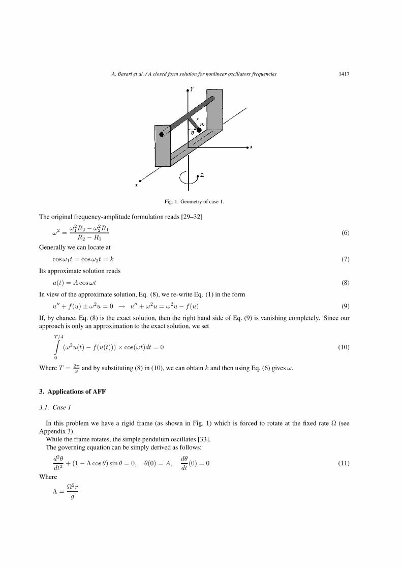
Fig. 1. Geometry of case 1.
The original frequency-amplitude formulation reads [29–32]
ω2 =ω2
1R2 − ω22R1
R2 − R1(6)
Generally we can locate at
cosω1t = cosω2t = k (7)
Its approximate solution reads
u(t) = A cosωt (8)
In view of the approximate solution, Eq. (8), we re-write Eq. (1) in the form
u′′ + f(u) ± ω2u = 0 → u′′ + ω2u = ω2u − f(u) (9)
If, by chance, Eq. (8) is the exact solution, then the right hand side of Eq. (9) is vanishing completely. Since ourapproach is only an approximation to the exact solution, we set
T/4∫0
(ω2u(t) − f(u(t))) × cos(ωt)dt = 0 (10)
Where T = 2πω and by substituting (8) in (10), we can obtain k and then using Eq. (6) gives ω.
3. Applications of AFF
3.1. Case 1
In this problem we have a rigid frame (as shown in Fig. 1) which is forced to rotate at the fixed rate Ω (seeAppendix 3).
While the frame rotates, the simple pendulum oscillates [33].The governing equation can be simply derived as follows:
d2θ
dt2+ (1 − Λ cos θ) sin θ = 0, θ(0) = A,
dθ
dt(0) = 0 (11)
Where
Λ =Ω2r
g
1418 A. Barari et al. / A closed form solution for nonlinear oscillators frequencies
The centrifugal acceleration from rotating reference frames can be used which is a readily-observable physicalfact. The magnitude and direction of the centrifugal acceleration varies from place to place in the rotating frame.Therefore it is called the centrifugal field which is zero at the pivot. It should be noted that, by going farther from thepivot, the centrifugal acceleration increases. It is everywhere directed radially outwards from the pivot. Centrifugalforce has relation with Coriolis force in rotating frameworks [34,35].
Pendulums require great mechanical stability: a length change of only 0.02%, 1/5 millimeter in a clock pendulum,will cause an error of a minute per week [36].
3.1.1. Solution of case 1 using frequency formulationThe above mentioned approach is applied herein to the non-linear differential equation introduced. The equation
takes the form
d2
dt2u(t) + (1 − Λ cosu(t)) sin u(t) = 0 (12)
Most useful trial-functions are [37]
u1(t) = A cos t (13)
u2(t) = A cos 2t (14)
Substituting u1 , u2 in Eq. (12) separately results in R1 , R2:
R1(t) =d2
dt2(A cos t) + (1 − Λ cos(A cos t)) sin(A cos t) =
(15)−A cos t + (1 − Λ cos(A cos t) sin(A cos t))
And
R2(t) =d2
dt2(A cos 2t) + (1 − Λ cos(A cos 2t)) sin(A cos 2t) =
(16)−4A cos 2t + (1 − Λ cos(A cos 2t) sin(A cos 2t))
So
ω2 =−4A cos 2t + (1 − Λ cos(A cos 2t)) sin(A cos 2t) + 4A cos t − 4(1 − Λ cos(A cos t) sin(A cos t)−4A cos 2t + (1 − Λ cos(A cos 2t)) sin(A cos 2t) + A cos t − (1 − Λ cos(A cos t) sin(A cos t)
(17)
Now we form this equation and put cos t = cos 2t = k, so:
R1 = −Ak + (1 − Λ cos(Ak)) sin(Ak) (18)
R2 = −4Ak + (1 − Λ cos(Ak)) sin(Ak) (19)
The period may be obtained as:
ω =
√− (−1 + Λ cos(Ak)) sin(Ak)
Ak(20)
Write the following integral as Eq. (10):T4∫
0
⎡⎣⎛⎝⎛⎝−
(−1 + Λ cos(Ak)) sin(Ak) × cos(√
− (−1+Λcos(Ak)) sin(Ak)Ak × t)
k
⎞⎠
−(
1 − Λ cos
(A cos
(√− (−1 + Λ cos(Ak)) sin(Ak)
Ak× t
)))× (21)
sin
(A cos
(√− (−1 + Λ cos(Ak)) sin(Ak)
Ak× t
)))× cos
√− (−1 + Λ cos(Ak)) sin(Ak)
Akt
]dt
A. Barari et al. / A closed form solution for nonlinear oscillators frequencies 1419
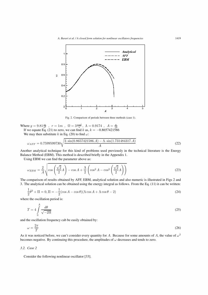
Fig. 2. Comparison of periods between three methods (case 1).
Where g = 9.81 ms2 , r = 1m , Ω = 3 rad
s , Λ = 0.9174 , A = π18
If we equate Eq. (21) to zero, we can find k as, k = −0.8657421586We may then substitute k in Eq. (20) to find ω:
ωAFF = 0.7599599730
√2. sin(0.8657421586.A)− Λ. sin(1.731484317.A)
A(22)
Another analytical technique for this kind of problems used previously in the technical literature is the EnergyBalance Method (EBM). This method is described briefly in the Appendix 1.
Using EBM we can find the parameter above as:
ωEBM =2A
√√√√cos
(√2
2A
)− cosA +
Λ2
(cos2 A − cos2
(√2
2A
))(23)
The comparison of results obtained by AFF, EBM, analytical solution and also numeric is illustrated in Figs 2 and3. The analytical solution can be obtained using the energy integral as follows. From the Eq. (11) it can be written:
12θ2 + Π = 0, Π = −1
2(cosA − cos θ)(Λ cosA + Λ cos θ − 2) (24)
where the oscillation period is:
T = 4
A∫0
dθ√−2Π(25)
and the oscillation frequency cab be easily obtained by:
ω =2π
T(26)
As it was noticed before, we can’t consider every quantity for A. Because for some amounts of A, the value of ω2
becomes negative. By continuing this procedure, the amplitudes of ω decreases and tends to zero.
3.2. Case 2
Consider the following nonlinear oscillator [33].
1420 A. Barari et al. / A closed form solution for nonlinear oscillators frequencies
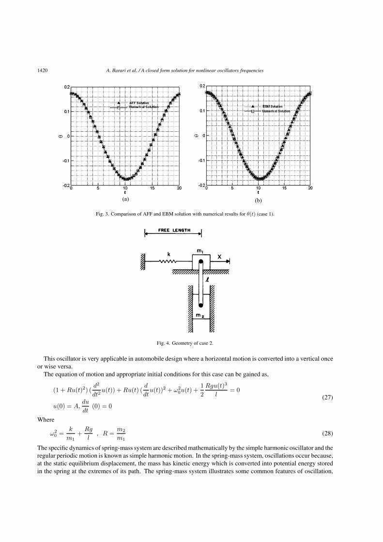
(a) (b)
Fig. 3. Comparison of AFF and EBM solution with numerical results for θ(t) (case 1).
Fig. 4. Geometry of case 2.
This oscillator is very applicable in automobile design where a horizontal motion is converted into a vertical onceor wise versa.
The equation of motion and appropriate initial conditions for this case can be gained as,
(1 + Ru(t)2) (d2
dt2u(t)) + Ru(t) (
d
dtu(t))2 + ω2
0u(t) +12
Rgu(t)3
l= 0
(27)u(0) = A,
du
dt(0) = 0
Where
ω20 =
k
m1+
Rg
l, R =
m2
m1(28)
The specific dynamics of spring-mass system are described mathematically by the simple harmonic oscillator and theregular periodic motion is known as simple harmonic motion. In the spring-mass system, oscillations occur because,at the static equilibrium displacement, the mass has kinetic energy which is converted into potential energy storedin the spring at the extremes of its path. The spring-mass system illustrates some common features of oscillation,
A. Barari et al. / A closed form solution for nonlinear oscillators frequencies 1421
namely the existence of equilibrium and the presence of a restoring force getting stronger when the system deviatesfrom equilibrium.
3.2.1. Solution of case 2 using AFFAccording to He’s amplitude frequency formulation we choose two trial functions: u1(t) = A cos(t) , u2(t) =
A cos(2t) substituting u1, u2 into Eq. (27) we obtain, respectively, the following residuals:
R1 = (1 + RA2 cos2 t)(
d2
dt2(A cos t)
)+ RA cos t
(d
dt(A cos t)2
)+ ω0A cos t
(29)
+RgA3 cos3 t
l− (1 + RA2 cos2 t)A cos t + RA3 cos t sin2 t + ω0A cos t
And
R2 = (1 + RA2 cos2 2t)(
d2
dt2(A cos 2t)
)+ RA cos t
(d
dt(A cos 2t)2
)+ ω0A cos 2t
(30)
+RgA3 cos3 2t
l− (1 + RA2 cos2 2t)A cos 2t + RA3 cos 2t sin2 2t + ω0A cos 2t
The angular rate is:
ω2 = (−4(1 + RA2 cos(2t)2)A cos(2t) + 4RA3 cos(2t) sin(2t)2
+ω20A cos(2t) +
12
RgA3 cos(2t)3
l+ 4(1 + RA2 cos(t)2)A cos(t) − 4RA3 cos(t)
sin(t)2 − 4ω20A cos(t) − 2RgA3 cos(t)3
l)/(−4(1 + RA2 cos(2t)2)A cos(2t) (31)
+4RA3 cos(2t) sin(2t)2 + ω20A cos(2t) +
12
RgA3 cos(2t)3
l
+(1 + RA2 cos(t)2)A cos(t) − RA3 cos(t) sin(t)2 − ω20A cos(t) − 1
2RgA3 cos(t)3
l)
Now we form this equation and put cos t = cos 2t = k, so:
ω =
√2√
2ω20 l+RgA2k2
l(1+2RA2k2−RA2)
2(32)
We choose u(t) = A cos(ωt) and put it into the Eqs (10) and (27), then we determine the following integral:
T/4∫0
⎡⎢⎣⎛⎜⎝⎛⎜⎝1 + RA2 cos
⎛⎝√
2√
2ω20l+RgA2k2
l(1+2RA2k2−RA2)×t
2
⎞⎠
2⎞⎟⎠⎛⎝ d2
dt2
⎛⎝A cos
⎛⎝√
2√
2ω20 l+RgA2k2
l(1+2RA2k2−RA2)×t
2
⎞⎠⎞⎠⎞⎠
+RA cos
⎛⎝√
2√
2ω20 l+RgA2k2
l(1+2RA2k2−RA2) × t
2
⎞⎠⎛⎝ d
dt
⎛⎝A cos
⎛⎝⎛⎝1
2
⎛⎝√
2√
2ω20l+RgA2k2
l(1+2RA2k2−RA2)×t
2
⎞⎠⎞⎠⎞⎠⎞⎠ (33)
+ω20A cos
⎛⎝√
2√
2ω20 l+RgA2k2
l(1+2RA2k2−RA2)×t
2
⎞⎠+
12
RgA3 cos(√
2
√2ω2
0l+RgA2k2
l(1+2RA2k2−RA2)×t
2 )3
l
⎞⎟⎟⎠× cos(ωt)
⎤⎥⎥⎦ dt
Where g = 9.81 ms2 , k = 200N
m , m1 = 10kg, m2 = 1kg, l = 0.5m, A = 0.5 tan π18
We can find k if we put Eq. (33) equal zero. So we have:
1422 A. Barari et al. / A closed form solution for nonlinear oscillators frequencies
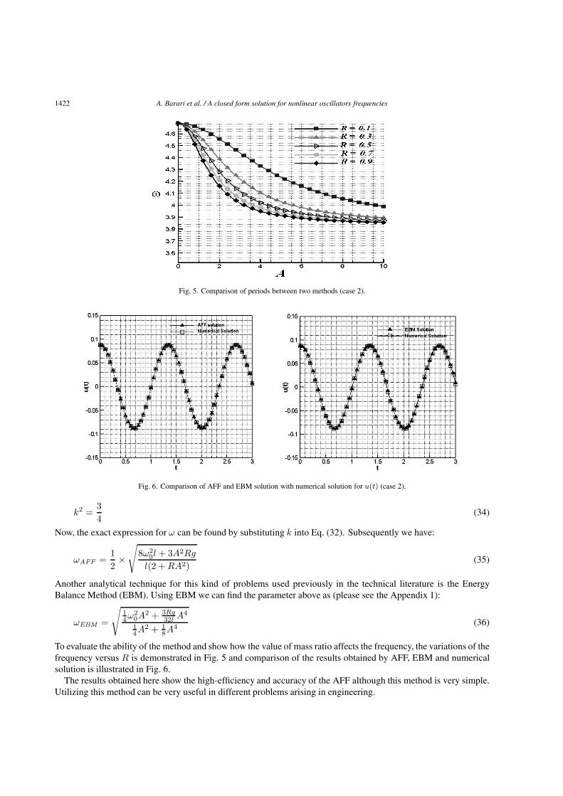
Fig. 5. Comparison of periods between two methods (case 2).
Fig. 6. Comparison of AFF and EBM solution with numerical solution for u(t) (case 2).
k2 =34
(34)
Now, the exact expression for ω can be found by substituting k into Eq. (32). Subsequently we have:
ωAFF =12×√
8ω20l + 3A2Rg
l(2 + RA2)(35)
Another analytical technique for this kind of problems used previously in the technical literature is the EnergyBalance Method (EBM). Using EBM we can find the parameter above as (please see the Appendix 1):
ωEBM =
√14ω2
0A2 + 3Rg
32l A4
14A2 + 1
8A4(36)
To evaluate the ability of the method and show how the value of mass ratio affects the frequency, the variations of thefrequency versus R is demonstrated in Fig. 5 and comparison of the results obtained by AFF, EBM and numericalsolution is illustrated in Fig. 6.
The results obtained here show the high-efficiency and accuracy of the AFF although this method is very simple.Utilizing this method can be very useful in different problems arising in engineering.
A. Barari et al. / A closed form solution for nonlinear oscillators frequencies 1423
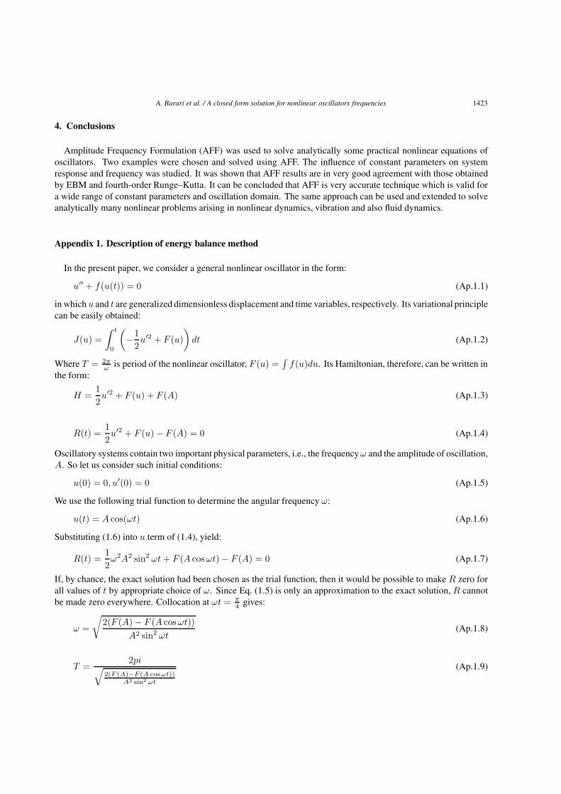
4. Conclusions
Amplitude Frequency Formulation (AFF) was used to solve analytically some practical nonlinear equations ofoscillators. Two examples were chosen and solved using AFF. The influence of constant parameters on systemresponse and frequency was studied. It was shown that AFF results are in very good agreement with those obtainedby EBM and fourth-order Runge–Kutta. It can be concluded that AFF is very accurate technique which is valid fora wide range of constant parameters and oscillation domain. The same approach can be used and extended to solveanalytically many nonlinear problems arising in nonlinear dynamics, vibration and also fluid dynamics.
Appendix 1. Description of energy balance method
In the present paper, we consider a general nonlinear oscillator in the form:
u′′ + f(u(t)) = 0 (Ap.1.1)
in which u and t are generalized dimensionless displacement and time variables, respectively. Its variational principlecan be easily obtained:
J(u) =∫ t
0
(−1
2u′2 + F (u)
)dt (Ap.1.2)
Where T = 2πω is period of the nonlinear oscillator, F (u) =
∫f(u)du. Its Hamiltonian, therefore, can be written in
the form:
H =12u′2 + F (u) + F (A) (Ap.1.3)
R(t) =12u′2 + F (u) − F (A) = 0 (Ap.1.4)
Oscillatory systems contain two important physical parameters, i.e., the frequencyω and the amplitude of oscillation,A. So let us consider such initial conditions:
u(0) = 0, u′(0) = 0 (Ap.1.5)
We use the following trial function to determine the angular frequency ω:
u(t) = A cos(ωt) (Ap.1.6)
Substituting (1.6) into u term of (1.4), yield:
R(t) =12ω2A2 sin2 ωt + F (A cosωt) − F (A) = 0 (Ap.1.7)
If, by chance, the exact solution had been chosen as the trial function, then it would be possible to make R zero forall values of t by appropriate choice of ω. Since Eq. (1.5) is only an approximation to the exact solution, R cannotbe made zero everywhere. Collocation at ωt = π
4 gives:
ω =
√2(F (A) − F (A cos ωt))
A2 sin2 ωt(Ap.1.8)
T =2pi√
2(F (A)−F (A cos ωt))A2 sin2 ωt
(Ap.1.9)
1424 A. Barari et al. / A closed form solution for nonlinear oscillators frequencies
Appendix 2. Description of RK4
The Runge-Kutta method is used to solve differential equation systems [38]. Second order differential equationscan be usually changed into first order equations and then are solved through Runge-Kutta method:
Consider an initial value problem as follows:
y′ = f(t, y), y(t0) = y0. (Ap.2.1)
Then RK4 method is given for this problem as below:
yn+1 = yn +16h(k1 + 2k2 + 2k3 + k4), (Ap.2.2)
tn+1 = tn + h (Ap.2.3)
Where yn+1 is the RK4 approximation of y(tn+1) and
k1 = f(tn, yn), (Ap.2.4)
k2 = f
(tn +
12h, yn +
12hk1
)(Ap.2.5)
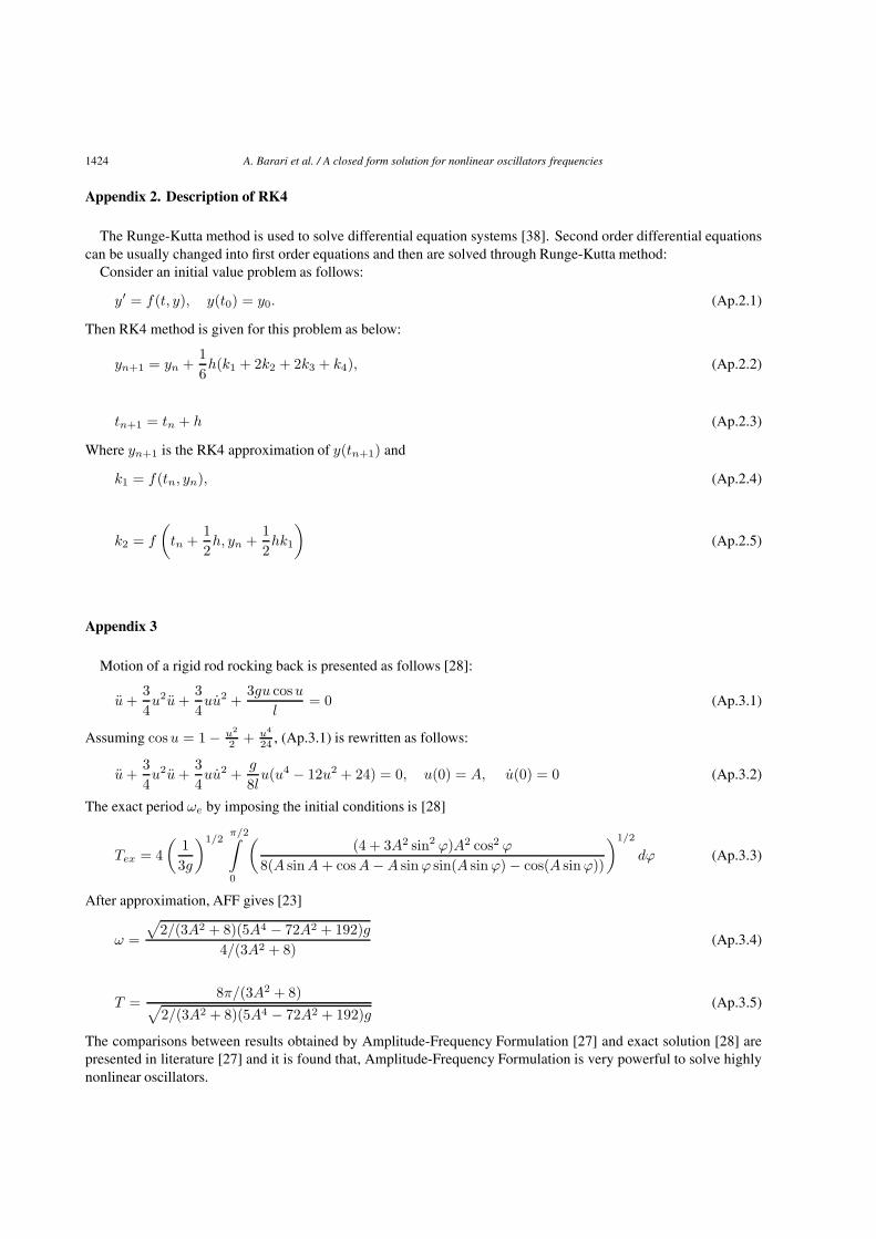
Appendix 3
Motion of a rigid rod rocking back is presented as follows [28]:
u +34u2u +
34uu2 +
3gu cosu
l= 0 (Ap.3.1)
Assuming cosu = 1 − u2
2 + u4
24 , (Ap.3.1) is rewritten as follows:
u +34u2u +
34uu2 +
g
8lu(u4 − 12u2 + 24) = 0, u(0) = A, u(0) = 0 (Ap.3.2)
The exact period ωe by imposing the initial conditions is [28]
Tex = 4(
13g
)1/2π/2∫0
((4 + 3A2 sin2 ϕ)A2 cos2 ϕ
8(A sin A + cosA − A sin ϕ sin(A sin ϕ) − cos(A sin ϕ))
)1/2
dϕ (Ap.3.3)
After approximation, AFF gives [23]
ω =
√2/(3A2 + 8)(5A4 − 72A2 + 192)g
4/(3A2 + 8)(Ap.3.4)
T =8π/(3A2 + 8)√
2/(3A2 + 8)(5A4 − 72A2 + 192)g(Ap.3.5)
The comparisons between results obtained by Amplitude-Frequency Formulation [27] and exact solution [28] arepresented in literature [27] and it is found that, Amplitude-Frequency Formulation is very powerful to solve highlynonlinear oscillators.
A. Barari et al. / A closed form solution for nonlinear oscillators frequencies 1425
References
[1] B.S. Lazarov, M. Schevenels and O. Sigmund, Robust design of large-displacement compliant mechanisms, Mechanical sciences 2 (2011),175–182.
[2] D.D. Ganji and S.H. Hashemi Kachapi, Analysis of nonlinear equations in fluids, Progress in Nonlinear Science 2 (2011), 1–293.[3] D.D. Ganji and S.H. Hashemi Kachapi, Analytical and numerical methods in engineering and applied sciences, Progress in Nonlinear
Science 3 (2011), 1–579.[4] M.G. Sfahani, A. Barari, M. Omidvar, S.S.Ganji and G. Domairry, Dynamic response of inextensible beams by improved Energy Balance
Method, Proceedings of the Institution of Mechanical Engineers, Part K: Journal of Multi-body Dynamics 225(1) (2011), 66–73.[5] L.B. Ibsen, A. Barari and A. Kimiaeifar, Analysis of highly nonlinear oscillation systems using He’s max-min method and comparison
with homotopy analysis and energy balance methods, Sadhana 35 (2010), 1–16.[6] S.-Q. Wang and J.-H. He, Nonlinear oscillator with discontinuity by parameter-expansion method, Chaos Solitons and Fractals 35 (2008),
688–691.[7] J.H. He, Comment on “He’s frequency formulation for nonlinear oscillators”, Eur J Phys 29 (2008), L1–L4.[8] J. Huan He, An improved amplitude-frequency formulation for nonlinear oscillators, Int J Nonlinear Sciences and Numerical Simulation
9(2) (2008), 211–212.[9] D. Younesian, H. Askari, Z. Saadatnia and M.K. Yazdi, Periodic solutions for nonlinear oscillation of a centrifugal governor system using
the He’s frequency-amplitude formulation and He’s energy balance method, Nonlinear Sci Lett A 2(3) (2011), 143–149.[10] A. Fereidoon, M. Ghadimi, A. Barari, H.D. Kaliji andG. Domairry, Nonlinear Vibration of Oscillation Systems Using Frequency-Amplitude
Formulation, Shock and Vibration, 2011, 18, 1–10, DOI: 10.3233/SAV20100633.[11] A. Barari, M. Omidvar, A.R. Ghotbi and D.D. Ganji, Application of homotopy perturbation method and variational iteration method to
nonlinear oscillator differential equations, Acta Applicandae Mathematicae 104 (2008), 161–171.[12] M. Miansari, M. Miansari, A. Barari and G. Domairry, Analysis of Blasius Equation for Flat-Plate Flow with Infinite Boundary Value,
International Journal for Computational Methods in Engineering Science and Mechanics 11(2) (2010), 79–84.[13] M.G. Sfahani, S.S. Ganji, A. Barari, H. Mirgolbabaei and G. Domairry, Analytical Solutions to Nonlinear Conservative Oscillator with
Fifth-Order Non-linearity, Earthquake Engineering and Engineering Vibration 5(3) (2010), 367–374.[14] M. Omidvar, A. Barari, M. Momeni and D.D. Ganji, New Class of Solutions for Water Infiltration Problems in Unsaturated Soils,
Geomechanics and Geoengineering: An International Journal 5(2) (2010), 127–135.[15] F. Fouladi, E. Hosseinzadeh, A. Barari and G. Domairry, Highly Nonlinear Temperature Dependent Fin Analysis by Variational Iteration
Method, Journal of Heat Transfer Research 41(2), 155–165.[16] A. Barari, M. Omidvar and D.D. Ganji, Tahmasebi Poor A., An Approximate solution for boundary value problems in structural engineering
and fluid mechanics, Journal of Mathematical Problems in Engineering (2008), Article ID 394103, 1–13.[17] H.L. Zhang, Application of He’s frequency-amplitude formulation to a force nonlinear oscillator, International Journal of Nonlinear
Science and Numerical Simulation 9(3) (2008), 297–300.[18] L. Geng and X.C. Cai, He’s frequency formulation for nonlinear oscillators, European Journal of Physics 28 (2007), 923–931.[19] D.H. Shou and J.H. He, Application of parameter expansion method to strongly nonlinear oscillator, International Journal of Nonlinear
Science and Numerical Simulation 8 (2007), 121–124.[20] W.P. Sun, B.S. Wu and C.W. Lim, Approximate analytical solutions for oscillation of a mass attached to a stretched elastic wire, J of Sound
and Vib 300 (2007), 1042–1047.[21] S. Durmaz, S.A. Demirbag and M.O. Kaya, Approximate solutions for a nonlinear oscillator of a mass attached to a stretched elastic wire,
Computer and Mathematics with applications 61 (2011), 578–585.[22] M.O. Kaya, S. Durmaz and S.A. Demirbag, He’s variational approach to multiple coupled nonlinear oscillators, International Journal of
Non-Linear Sciences and Numerical Simulation 11(10) (2010), 859–865.[23] Milham, Willis I, Time and Timekeepers, MacMillan, 1945, pp. 188–194.[24] Glasgow, David, Watch and Clock Making. London: Cassel and Co. 1885, pp. 279–284.[25] Beckett, Edmund (Lord Grimsthorpe), A Rudimentary Treatise on Clocks and Watches and Bells, 6th ed., London: Lockwood and Co...
1874, p. 50.[26] H. Sherryl, Stovall Basic Inertial Navigation, Naval Air Warfare Center Weapons Division, September 1997.[27] S.S. Ganji, D.D. Ganji, H. Babazadeh and N. Sadoughi, Application of amplitude-frequency formulation to nonlinear oscillation system
of the motion of a rigid rod rocking back, Mathematical Methods in Applied Sciences 33 (2010), 157–166.[28] B.S. Wu, C.S. Lim and L.H. He, A new method for approximate analytical solutions to nonlinear oscillations of nonnatural systems,
Nonlinear Dynamics 32 (2003), 1–13.[29] J.H. He, Some asymptotic methods for strongly nonlinear equations, Int J Mod Phys B 20 (2006), 1141–1199.[30] J.H. He, Nonperturbative methods for strongly nonlinear problems, dissertation.de-Verlag im Internet GmbH, 2006.[31] A. Kimiaeifar, O. T. Thomsen and E. Lund, Assessment of HPM with HAM to find an analytical solution for the steady flow of the third
grade fluid in a porous half space, IMA Journal of Applied Mathematics (2011) 76(2), 326–339.[32] A. Kimiaeifar, An analytical approach to investigate the response and stability of Van der Pol-Mathieu-Duffing oscillators under different
excitation functions, Journal of Mathematical Methods in the Applied Sciences 33 (2010), 1571–1577.[33] A.H. Nayfeh and D.T. Mook, Nonlinear Oscillations, Wiley, New York, 1979.[34] S.T. Thornton and J.B. Marion, Classical Dynamics of Particles and Systems (5th ed.), Belmont CA: Brook/Cole. Chapter 10. 2004. ISBN
0534408966.[35] Federal Aviation Administration, Pilot’s Encyclopedia of Aeronautical Knowledge. Oklahoma City OK: Skyhorse Publishing Inc. Figure
3–21, 2007. ISBN 1602390347.[36] D. Halliday, R. Resnick and J. Walker, Fundamentals of Physics, 5th ed., New York: John Wiley and Sons, 1997, p. 381. ISBN 0471148547.
1426 A. Barari et al. / A closed form solution for nonlinear oscillators frequencies
[37] J.-H. He, An Improved Amplitude-frequency Formulation for Nonlinear Oscillators, International Journal of Nonlinear Sciences andNumerical Simulation 9(2) (2008), 211–212.
[38] D.A. Anderson and J.C. Tannehill, Computational Fluid Mechanics and Heat Transfer, Hemisphere Publishing Corp, 1984.

International Journal of
AerospaceEngineeringHindawi Publishing Corporationhttp://www.hindawi.com Volume 2010
RoboticsJournal of
Hindawi Publishing Corporationhttp://www.hindawi.com Volume 2014
Hindawi Publishing Corporationhttp://www.hindawi.com Volume 2014
Active and Passive Electronic Components
Control Scienceand Engineering
Journal of
Hindawi Publishing Corporationhttp://www.hindawi.com Volume 2014
International Journal of
RotatingMachinery
Hindawi Publishing Corporationhttp://www.hindawi.com Volume 2014
Hindawi Publishing Corporation http://www.hindawi.com
Journal ofEngineeringVolume 2014
Submit your manuscripts athttp://www.hindawi.com
VLSI Design
Hindawi Publishing Corporationhttp://www.hindawi.com Volume 2014
Hindawi Publishing Corporationhttp://www.hindawi.com Volume 2014
Shock and Vibration
Hindawi Publishing Corporationhttp://www.hindawi.com Volume 2014
Civil EngineeringAdvances in
Acoustics and VibrationAdvances in
Hindawi Publishing Corporationhttp://www.hindawi.com Volume 2014
Hindawi Publishing Corporationhttp://www.hindawi.com Volume 2014
Electrical and Computer Engineering
Journal of
Advances inOptoElectronics
Hindawi Publishing Corporation http://www.hindawi.com
Volume 2014
The Scientific World JournalHindawi Publishing Corporation http://www.hindawi.com Volume 2014
SensorsJournal of
Hindawi Publishing Corporationhttp://www.hindawi.com Volume 2014
Modelling & Simulation in EngineeringHindawi Publishing Corporation http://www.hindawi.com Volume 2014
Hindawi Publishing Corporationhttp://www.hindawi.com Volume 2014
Chemical EngineeringInternational Journal of Antennas and
Propagation
International Journal of
Hindawi Publishing Corporationhttp://www.hindawi.com Volume 2014
Hindawi Publishing Corporationhttp://www.hindawi.com Volume 2014
Navigation and Observation
International Journal of
Hindawi Publishing Corporationhttp://www.hindawi.com Volume 2014
DistributedSensor Networks
International Journal of