A Climatology of Wintertime Barrier Winds off Southeast

A Climatology of Wintertime Barrier Winds off Southeast Greenland

B. E. HARDEN AND I. A. RENFREW

University of East Anglia, Norwich, United Kingdom

G. N. PETERSEN

Icelandic Met Office, Reykjavik, Iceland

(Manuscript received 6 October 2010, in final form 23 February 2011)

ABSTRACT

A climatology of barrier winds along the southeastern coast of Greenland is presented based on 20 yr of

winter months (1989–2008) from the ECMWF Interim Reanalysis (ERA-Interim). Barrier wind events occur

predominantly at two locations: Denmark Strait North (DSN; 67.78N, 25.38W) and Denmark Strait South

(DSS; 64.98N, 35.98W). Events stronger than 20 m s21 occur on average once per week during winter with

considerable interannual variability—from 7 to 20 events per winter. The monthly frequency of barrier wind

events correlates with the monthly North Atlantic oscillation (NAO) index with a correlation coefficient of

0.57 (0.31) at DSN (DSS). The associated total turbulent heat fluxes for barrier wind events (area averaged)

were typically about 200 W m22 with peak values of 400 W m22 common in smaller regions. Area-averaged

surface stresses were typically between 0.5 and 1 N m22. Total precipitation rates were larger at DSS than

DSN, both typically less than 1 mm h21. The total turbulent heat fluxes were shown to have a large range as

a result of a large range in 2-m air temperature. Two classes of barrier winds—warm and cold—were in-

vestigated and found to develop in different synoptic-scale situations. Warm barrier winds developed when

there was a blocking high pressure over the Nordic seas, while cold barrier winds owed their presence to

a train of cyclones channeling through the region.

1. Introduction

Greenland presents a high, steep, and cold topographic

barrier to the atmosphere. Its ice sheet, which covers 80%

of the landmass, is responsible for the Greenland plateau

being higher than 3000 m above sea level. This large, cold

mass is capable of diverting and distorting atmospheric

flow around it, forcing a number of intermittent, low-

level, high-velocity wind events, such as westerly and

easterly tip jets (Doyle and Shapiro 1999; Moore 2003;

Moore and Renfrew 2005, hereafter MR05; Vage et al.

2009; Renfrew et al. 2009a; Outten et al. 2009, 2010),

barrier winds (MR05; Petersen et al. 2009) and katabatic/

downslope winds (Heinemann and Klein 2002; Klein

and Heinemann 2002). It also has influences on the de-

velopment of polar lows (Martin and Moore 2006), cy-

clogenesis (Petersen et al. 2003; Serreze et al. 1997),

cyclolysis (Hoskins and Hodges 2002; Serreze et al.

1997), and the properties of cyclones that pass through

the region (Kristjansson and McInnes 1999; Skeie et al.

2006).

Not only are the low-level wind events produced by

Greenland responsible for some of the stormiest seas in

the world’s oceans (Sampe and Xie 2007; Moore et al.

2008) producing hazardous maritime conditions, but

interest has been piqued recently into the possible in-

fluence that these intermittent events have on the ocean

in a region that is vital for the thermohaline circulation.

For example, westerly tip jets (produced around the

southern tip of Greenland) have been shown to be ca-

pable of triggering deep convection in the Irminger Sea

(Pickart et al. 2003; Vage et al. 2008). The knowledge

that intense, but intermittent, wind phenomena can have

a protracted impact on the slow overturning circulation

of the Atlantic Ocean points to the importance of un-

derstanding the prevalent atmospheric conditions and

ocean forcing in the region.

The subject of this study is barrier winds—low-level

jets produced when air is forced toward a high and

Corresponding author address: Benjamin Harden, School of

Environmental Sciences, University of East Anglia, Norwich NR4

7TJ, United Kingdom.

E-mail: [email protected]

1 SEPTEMBER 2011 H A R D E N E T A L . 4701

DOI: 10.1175/2011JCLI4113.1

� 2011 American Meteorological Society

steep topographic barrier (such as Greenland) with a

large nondimensional mountain height, Nh/U, where N is

the Brunt–Vaisala frequency, h is the mountain height,

and U is the upstream wind speed (Schwerdtfeger 1975;

Parish 1983; Pierrehumbert and Wyman 1985). The air,

unable to ascend the barrier, is dammed and a pressure

gradient perpendicular to the barrier develops, leading

to geostrophic flow along the barrier (to first order).

When the upstream winds are produced by a synoptic-

scale cyclone, the separation of ‘‘synoptic’’ and ‘‘pertur-

bation’’ pressure gradients is difficult (e.g., see Petersen

et al. 2009). Barrier winds have been studied in situ and

through numerical models at numerous mountainous

locations around the world; the Antarctic Peninsula

(Schwerdtfeger 1975; Parish 1983), Alaska (Loescher

et al. 2006; Olson and Colle 2009), California (Cui et al.

1998), New Zealand (Revell et al. 2002), the Rockies

(Colle and Mass 1995), the Sierra Nevada (Parish 1982),

the Appalachians (Bell and Bosart 1988), and the Alps

(Chen and Smith 1987), plus have been the subject of a

number of idealized numerical studies (Braun et al. 1999;

Petersen et al. 2003, 2005).

Along the coast of Greenland, barrier wind events

were comprehensively observed by instrumented air-

craft during the Greenland Flow Distortion Experiment

(GFDex) field campaign (Renfrew et al. 2008). Petersen

et al. (2009) provide an overview of two barrier wind

events, including jet cross sections from dropsonde

soundings, numerical simulations, and trajectory analy-

sis. They showed that the presence of Greenland caused

up to a doubling in the maximum wind speed along

the coastline—with the precise synoptic-scale situation

being critical for the location and magnitude of the as-

sociated barrier winds. GFDex showed how potentially

important these winds could be for the ocean. In the two

and a half weeks of the field campaign, three barrier

wind events were observed; in one case, measured total

turbulent heat fluxes exceeded 600 W m22 and surface

stresses reached 1.5 N m22 (Renfrew et al. 2009b).

An investigation of their effects on the ocean was

conducted through very high-resolution numerical mod-

eling of the Irminger Sea and Denmark Strait by Haine

et al. (2009). They showed that these barrier winds were

capable of producing maximum net heat fluxes of around

600 W m22 and a peak current of nearly 2 m s21, and

that the boundary layer depth of the ocean responds

rapidly and sensitively with mean values of around 100 m

but with maximum values as large as 500 m. Recently,

Straneo et al. (2010) showed that strong barrier winds

off southeast Greenland are likely responsible for the

recirculation of warm water up glacial fjords, increasing

the melting of glaciers at their base and enhancing the

speed of their descent into the ocean.

Tip jets and barrier winds around Greenland were

the subject of the Quick Scatterometer (QuikSCAT)

climatology of MR05. MR05 provided much useful in-

formation about strong wind events in the region but

was limited by only having a 5-yr record over the ice-free

oceans and only for 10-m winds. A lack of wind speed

data over sea ice affects a large region in the north of

Denmark Strait, where barrier winds are known to occur

(Petersen et al. 2009). Tip jets have recently been the

subject of climatologies using atmospheric reanalysis

products (Sproson et al. 2008; Vage et al. 2009), but

climatological knowledge of barrier winds in the region

is still limited to that provided by MR05. Here we build

upon that by compiling a climatology of barrier winds

using state-of-the-art meteorological reanalyses, thus

making use of a number of diagnostics throughout the

atmosphere as well as over land and sea ice.

The aims of this study are summarized as follows:

d To extend knowledge about the frequency, strength,

location, and properties of barrier winds in the region.d To outline the impact these winds could be having on

the ocean, providing the oceanic community with a

useful tool for studying atmospheric forcing in the

region.

2. Data

a. Description

Data from the European Centre for Medium-Range

Weather Forecasts (ECMWF) Interim Reanalysis (ERA-

Interim) (Berrisford et al. 2009) were used for this study.

ERA-Interim is a global reanalysis product that covers

the period from 1989 to the present. A number of im-

provements have been made on its predecessor, the 40-yr

ECMWF Re-Analysis (ERA-40). These include many

model refinements along with changes in data assimilation;

most significantly, a four-dimensional variational data as-

similation (4D-Var) process is now used (Rabier et al. 1998).

The underlying model for ERA-Interim is ECMWF’s

Integrated Forecast System (IFS) cycle 31r2. This is

a spectral, semi-implicit, semi-Lagrangian model with

255 spectral modes (T255) and 60 levels (L60) in the

vertical. For gridpoint fields, a reduced Gaussian grid is

used with an approximately uniform spacing of 80 km

(N128). This is a marked improvement on ERA-40,

which was T159, L60, and N80, so an approximate hor-

izontal resolution of 125 km. The improvement in hor-

izontal resolution is crucial, for this study, to adequately

resolve the relatively small-scale barrier winds. The at-

mosphere is coupled to an ocean wave model with 30

wave frequencies that can propagate in 24 directions.

4702 J O U R N A L O F C L I M A T E VOLUME 24

Reanalysis fields are produced 4 times daily at 0000,

0600, 1200, and 1800 UTC. Ten-day forecasts are run

twice a day, initialized at 0000 and 1200 UTC. Data are

available on the 60 model levels or, as used here, in-

terpolated onto 37 pressure levels.

b. Verification

To appreciate the strengths and limitations of ERA-

Interim, a verification of the output against observations

is necessary. In the region of interest for this study (the

subpolar seas of the North Atlantic), work has already

been conducted to verify ECMWF products (Renfrew

et al. 2002; Vage et al. 2009; Renfrew et al. 2009b). These

studies were conducted under similar meteorological

conditions to those of this study, which makes their find-

ings particularly pertinent. These studies were examining

ERA-40 and ECMWF operational analyses (not ERA-

Interim); however, the underlying model dynamics are

largely the same, so much of this verification should be

applicable here. ECMWF products were found to per-

form reasonably well at the surface; however, high wind

speed events were underrepresented in coarse-resolution

models by up to 5 m s21 (Vage et al. 2009; Renfrew et al.

2009b), near-surface temperatures had a systematic cold

bias of around 1 K, and the resulting heat fluxes were

observed to be too large by 10% (Renfrew et al. 2009b).

To confirm that these findings are relevant to ERA-

Interim, further verification is now presented.

Near-surface meteorological variables were collected

during a research cruise in the Irminger Sea aboard the

R/V Knorr in October 2008 (KN194–4). Specifically,

pressure and wind speed measured by the Improved

FIG. 1. (left) Comparison of time series for ERA-Interim (thin) near-surface fields with measurements made

aboard the R/V Knorr in the Irminger Sea in October 2008 (thick). (right) All data points plotted on scatterplots.

Thin line is perfect agreement; thick line is best linear fit to the data. (a),(b) Surface pressure (hPa); (c),(d) 10-m wind

speed (m s21); and (e),(f) 2-m temperature (8C). (d) Crosses are data points recorded before 20 Oct 2008 [dashed line

in (c)], circles are those after this date, thick dashed line is the linear regression for all data points recorded, and thick

solid line is the linear regression for all times before 20 October 2008 [dashed line in (c)].


Meteorological (IMET) package and temperature as

recorded by the Vaisala WXT5–10 system. All meteo-

rological instruments were mounted on a tower at the

bow of the ship, which put them 15.5 m above sea

level. In all subsequent analysis, the measurements are

extrapolated to the same heights as the outputs from

ERA-Interim—that is, to 10 m for wind speed, to 2 m

for temperature, and to the surface for pressure. This

was achieved using the logarithmic neutral profile for-

mulas for wind speed and temperature, and hydrostatic

balance for pressure. Stability-dependent surface-layer

formulas (Smith 1988) were also used for the wind speed

and temperature reductions but few discernible differ-

ences were seen. Because of an incomplete humidity

record, the neutral formulas were used.

A number of barrier winds were observed during the

October 2008 cruise, making this dataset ideal for verifying

the performance of ERA-Interim for this study. Figure 1

illustrates that surface pressure and the 10-m wind speed

from ERA-Interim compare well with data collected on

the Knorr. The ERA-Interim pressure, in particular, is

in excellent agreement with the measured pressure.

Strong winds are only slightly underrepresented in ERA-

Interim (mean bias is 21 m s21), indeed the product per-

forms better than was found in comparing ERA-40 wind

speeds with QuikSCAT (Vage et al. 2009). The thick

dashed trend line in Fig. 1d shows the regression for all

data points collected, but perhaps it is a little misleading.

It includes points recorded after 20 October 2008 (dashed

line in Fig. 1c), when the Knorr spent much of its time in

coastal regions where sheltering effects often lead to

stronger winds in the model than were recorded on the

Knorr. These latter points are shown in Fig. 1d with

circles, and the trend line excluding these points is

shown as the solid line in Fig. 1d. The conclusion is that

ERA-Interim represents 10-m winds well and better

than previous studies in which high wind speeds were

significantly underrepresented, for example, a mean bias

of 22.5 m s21 in Renfrew et al. (2009b).

The temperature comparison and trend line in Figs.

1e,f show that the 2-m temperature model field has

a cold bias of 28C, a feature seen by Renfrew et al.

(2009b) when comparing observations to the ECMWF

1.1258 operational analysis and which they attribute to

low model resolution—the feature was not there for the

same comparison with the ECMWF T511 resolution

model. As in that study, this is likely to produce an

overestimation of surface turbulent heat fluxes. Overall,

it seems that the performance of ERA-Interim at the

surface is good.

To be able to say how well ERA-Interim performs

with height, comparisons with radiosonde and dropsonde

observations in the region of interest were conducted.

Radiosondes were launched during the R/V Knorr

FIG. 2. Three sample radiosonde soundings (solid lines) made aboard the R/V Knorr in the Irminger Sea in

October 2008 and corresponding model soundings in the ERA-Interim dataset (dashed lines). Wind speed (thick,

m s21) and potential temperature (thin, K) shown.


cruise in October 2008. Figure 2 shows three represen-

tative soundings: during low-wind conditions (Fig. 2a)

and during barrier wind events (Figs. 2b,c). Under low

wind speed conditions, the winds are generally well

represented at all heights, while the cold bias seen at the

surface extends throughout the atmospheric column.

This cold bias is also observed at all heights under bar-

rier wind conditions. The magnitude of the maximum

wind speeds recorded during barrier wind conditions are

mostly well captured in the ERA-Interim product; al-

though, at some times, peak wind speeds are missed by

as much as 5 m s21. The jets were commonly observed to

be capped by a strong temperature inversion (e.g., in Fig.

2b), the gradients of which were poorly captured in the

model. This results in a model jet that is too broad in the

vertical. Figure 2c shows that when a barrier wind has

a weaker temperature inversion, the vertical gradients in

the measured wind speed are reduced and the perfor-

mance of ERA-Interim improves.

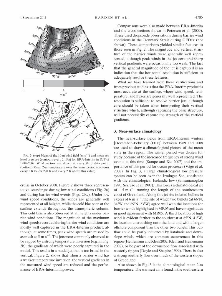
Comparisons were also made between ERA-Interim

and the cross sections shown in Petersen et al. (2009).

These used dropsonde observations during barrier wind

conditions in the Denmark Strait during GFDex (not

shown). These comparisons yielded similar features to

those seen in Fig. 2. The magnitude and vertical struc-

ture of the barrier winds were generally well repre-

sented, although peak winds in the jet core and sharp

vertical gradients were occasionally too weak. The fact

that the general magnitude of the jet is captured is an

indication that the horizontal resolution is sufficient to

adequately resolve these features.

What we have learned from these verifications and

from previous studies is that the ERA-Interim product is

most accurate at the surface, where wind speed, tem-

perature, and fluxes are generally well represented. The

resolution is sufficient to resolve barrier jets, although

care should be taken when interpreting their vertical

structure which, although capturing the basic structure,

will not necessarily capture the strength of the vertical

gradients.

3. Near-surface climatology

The near-surface fields from ERA-Interim winters

[December–February (DJF)] between 1989 and 2008

are used to draw a climatological picture of the mean

state in the region. The winter period was chosen for

study because of the increased frequency of strong wind

events at this time (Sampe and Xie 2007) and the im-

portance of this period for ocean processes (Vage et al.

2008). In Fig. 3, a large climatological low pressure

system can be seen over the Irminger Sea, consistent

with the climatological Icelandic low (Sahsamanoglou

1990; Serreze et al. 1997). This forces a climatological jet

of ;5 m s21 running the length of the southeastern

coast of Greenland. Along this jet sits isolated bullets in

excess of 6 m s21, the site of which two bullets (at 668N,

348W and 698N, 238W) agree well with the locations for

barrier winds highlighted in MR05 and have magnitudes

in good agreement with MR05. A third location of high

wind is evident farther to the southwest at 658N, 418W,

its location encroaching onto the land and with a larger

offshore component than the other two bullets. This out-

flow could be partly influenced by katabatic and down-

slope winds, which are common occurrences in this

region (Heinemann and Klein 2002; Klein and Heinemann

2002), or be part of the downslope flow associated with

westerly tip jets (Doyle and Shapiro 1999). There is also

a strong southerly flow over much of the western slopes

of Greenland.

Also shown in Fig. 3 is the climatological mean 2-m

temperature. The warmest air is found in the southeastern

FIG. 3. (top) Mean of the 10-m wind field (m s21) and mean sea

level pressure (contours every 2 hPa) for ERA-Interim in DJF of

1989–2008. Wind vectors are shown at every third data point.

(bottom) Mean 2-m temperature over the same period (contours

every 5 K below 270 K and every 2 K above this value).


part of the domain, reflecting the climatological sea

surface temperature pattern. The temperature decreases

to the north with the strongest gradient in temperature

over the ocean (the Arctic Front) occurring along the

southeastern Greenland coast, where the mean 2-m

temperature is below freezing in the region represented

by the climatological jet. The very low temperatures over

Greenland’s interior are due to the combined influences

of the ice sheet and altitude.

The fraction of time the wind speed exceeds 20 m s21

at each location in the domain is shown in Fig. 4. The

threshold of 20 m s21 was arbitrarily chosen as the

criterion for strong winds for this analysis, although

qualitatively similar patterns are seen for other thresh-

olds. This is a smaller threshold than used in MR05, but

it was chosen to take into consideration QuikSCAT’s

tendency to overestimate strong winds (e.g., Ebuchi

et al. 2002; Moore et al. 2008). As with the analysis of

MR05, three coastal locations of frequent high winds

are clear: two along Greenland’s southeastern coast

and a third at Cape Farewell. The two northerly lo-

cations correspond to the locations of frequent barrier

winds and the third location to frequent tip jets. At

each location, wind speeds exceed 20 m s21 more than

6% of the time, in some places as much as 10% of the

time.

In the remainder of this study, we focus on the two

northerly sites. See MR05, Sproson et al. (2008), and

Vage et al. (2009) for a climatological analysis of the

Cape Farewell site.

4. Barrier wind detection

a. Method

Barrier winds are characterized by strong winds di-

rected parallel to the coast . Therefore, in this study of

southeast Greenland, a barrier wind event is defined if at

any time the 10-m wind speed at a location is in excess of

a threshold wind speed and directed between northerly

(08N) and easterly (908N). Note that this pragmatic def-

inition does not take into account the flow dynamics, but

it is nonetheless useful in capturing what have previously

been shown to be barrier flows in the region (e.g. MR05,

Petersen et al. 2009). Furthermore, the proximity to the

steep topography of Greenland makes it very unlikely

that strong winds detected in this way will have been

produced without feeling the influence of the barrier in

some way.

Following MR05, the locations that will be used for

barrier wind detection are the two maxima in frequency of

high wind speed events (Fig. 4). These maxima correspond

to the Denmark Strait South (DSS) and Denmark Strait

North (DSN) locations identified in MR05 and for con-

sistency, the same nomenclature will be used here. Instead

of using a point measurement for detecting barrier winds

like MR05, a region that encompasses the maxima will be

used (marked by boxes in Fig. 4). These regions have been

selected to not include any land grid points.

The steps in the detection routine for each region are

as follows:

d At each time, the maximum 10-m wind speed in the

region, for which the wind direction is between north-

erly (08N) and easterly (908N), is found and a time

series is constructed from these values. Note that using

a larger range of wind directions resulted in a similar

number of detected events.d The maxima in this time series greater than 20 m s21

are selected. Different threshold values give qualita-

tively similar results.d Finally, for a maximum to be defined as a barrier wind

event, it must be distinct in time, that is, separate from

other maxima by more than 24 h. If wind speed

maxima greater than 20 m s21 are separated by less

than 24 h, then the time of the peak wind speed is

chosen.

b. Results

Applying the detection routine described above re-

sults in the detection of 252 barrier wind events at

DSS and 291 events at DSN over the 60-month period

(December–February between 1989 and 2008). This is

approximately one barrier wind event a week for each

FIG. 4. Percentage of time that the 10-m wind speed is in excess of

20 m s21 at each location in the domain for ERA-Interim in DJF of

1989–2008. Shading every 2%. Boxes mark the locations of DSS

and DSN. ERA-Interim orography is shown with contours; contour

interval is 1000 m.


location during these months. This can be compared to

Vage et al. (2009), who observed roughly one westerly tip

jet per two weeks in their ERA-40-based climatology. A

similar number of barrier events at each location are

slightly surprising, considering the difference in frequency

of high winds observed between the two locations in Fig. 4

(around 5% at DSS and 8% at DSN)—the implication

being that each event lasts longer at DSN than at DSS.

There exists a discrepancy between the mean frequency

of barrier wind events in this study and in MR05. The 47

barrier wind events detected by MR05 in 5 yr (one barrier

wind event a week) at DSS agrees well with the frequency

observed by this study, but MR05 observed only 19 events

at DSN. This discrepancy could be partly explained by the

point method of MR05 compared with the area method

used here; however, a more likely explanation is that

MR05 is based on measurements from QuikSCAT, which

cannot measure 10-m wind speeds above sea ice—this is

much more prevalent at DSN than at DSS.

To investigate interannual variability, Fig. 5 shows the

number of barrier wind events detected each month and

each winter season for the two locations. Both locations

experience a degree of year-to-year variability, but at

DSN it is larger (a standard deviation of 3.5 compared

with 2.4 at DSS). There is a reasonable correlation of

0.43 (0.64) between the number of barrier wind events at

each location each month (winter season). Looking at

individual months, it appears that no one month is par-

ticularly favored for the prevalence of barrier winds.

Also shown in Fig. 5 is the monthly and mean winter

(DJF) North Atlantic Oscillation (NAO) index of Hurrell

(1995). There is a positive correlation between the

monthly NAO index and the monthly frequency of bar-

rier wind events at both locations with correlation co-

efficients of 0.31 at DSS and 0.57 at DSN, both of which

are statistically significant at a 99% confidence level.

This is not entirely surprising considering high NAO

indices are forced by a deeper Icelandic low, the result of

more frequent and deeper cyclones, which are likely to

produce more and stronger barrier winds. Correlation

with the monthly southwestern Iceland mean sea level

pressure [used in calculating the NAO index of Hurrell

(1995)] yields a similar result but with slightly better

correlations—coefficients of 20.37 and 20.67 are found

at DSS and DSN, respectively. These correlations could

be useful in reconstructing barrier wind frequency for

times before meteorological reanalysis coverage, but for

which we have reliable NAO and mean sea level pres-

sure data.

It has been shown that there is a correlation between

the interannual variability at DSS and DSN. A sensible

question at this point seems to be, is there a causal re-

lationship between events at DSS and those at DSN?

Figure 6 shows how many events at DSS are succeeded

by an event at DSN within a certain lag time. It can

be seen that 30 of the 252 detected events at DSS are

concurrent with an event at DSN (approximately 12%).

The maximum in the figure (44 events) occurs at a lag

time of 6 h. This means that 17% of the time, an event

at DSS is succeeded by an event at DSN by 6 h. This

implies retrograde propagation of the event; the region

of strong winds travels northeastward up the coast

FIG. 5. (top),(middle) Number of barrier wind events detected per winter month (narrow

white bars) and winter season (gray bars); (top) is for DSN and (middle) is for DSS. (bottom)

NAO index by winter month (white bars) and winter season (gray bars).


(seemingly against the along-barrier flow). The reason

this lag exists is because of the common northeast-

ward propagation of cyclones through the region (e.g.,

Hoskins and Hodges 2002). It is logical to suggest that as

a cyclone moves through the region, an event is trig-

gered first at DSS and subsequently at DSN. This result

is evidence that barrier winds off Greenland are the

result of the direct influence of Greenland’s topography

on cyclones. The total number of events within 624 h of

the peak will give an upper limit on the number of

causally linked events because this period is typical of

the passage of a cyclone through the region. This crite-

rion results in 162 events (65%), meaning that the upper

limit of causally linked events is around two-thirds of the

total number of events at DSS.

The 2-m temperature was extracted for each event at

the DSN and DSS locations (Fig. 7). The thick dashed

line shows the climatological (DJF) mean for the two

locations (i.e., the boxes in Fig. 4). What is clear is that

the median barrier wind event temperature is not sig-

nificantly different from the climatological mean tem-

perature over the entire 60-month period of study at

each location. Around this mean value though, both

locations exhibit quite a large range. At DSS, much of

the variance is contained within a 4-K range of the me-

dian value, 274 K; however, temperatures can be as high

as 278 K or as low as 263 K in extreme cases. At DSN,

the temperatures are generally colder because of the

more northerly location of the region and also the in-

creased access to cold Arctic air that is available to the

northeast of the Denmark Strait. The distribution is

similar, although the range is somewhat larger; in par-

ticular, a cold tail is more exaggerated at DSN, with

temperatures lower than 255 K in extreme cases. Not

only are the median temperatures at each location com-

parable to their respective climatological means, but

the range of barrier wind temperatures is also compara-

ble to the climatological range observed throughout the

60-month period (not shown). This implies that barrier

winds bring about no special temperature regime; they

cannot be said to be generally ‘‘cold’’ or ‘‘warm’’ winds. A

further discussion of barrier wind temperatures is ad-

dressed later, in section 7.

5. Composite analysis

Mean composite fields have been produced for the 291

barrier winds detected at DSN and the 252 at DSS.

Looking first at the mean 10-m wind field in Fig. 8, we

can see that at both locations, the composite barrier

wind speed peaks at about 20 m s21 with a width of

200 km. The lengths of the composite barrier winds are

450 km at DSN and 700 km at DSS (as defined by the

15 m s21 contour). Importantly for DSS, much of the

region of strong winds is located upwind of the maxi-

mum, emphasizing the number of events at DSS that

occurs concurrently (or 6 a small time lag), with events

further upstream at DSN. Comparing with MR05’s

composites, the only substantial difference is that in this

study, the barrier wind composites are well defined over

FIG. 6. Histogram of lag time between barrier wind events at

DSS and DSN. A positive (negative) lag indicates that the event at

DSN occurred after (before) the event at DSS.FIG. 7. 2-m temperature (K) for all barrier wind events detected

at DSS and DSN. Thick horizontal line is the median, box indicates

first and third quartiles, and bars extend to the minimum and

maximum of the dataset. Crosses mark outliers defined as being 1.5

interquartile ranges outside of a quartile. Thick horizontal dashed

line is the climatological mean temperature for each region.


the sea ice, a feature that is especially important for

barrier winds at DSN.

The barrier winds at both locations are forced by

a composite low pressure of depth 980 hPa. For events

at DSS, the location of this low is over the western

Irminger Sea and for DSN it is farther to the northeast

off the west coast of Iceland. The translation of the

composite low is comparable to the translation of the

centers of peak wind speeds and is further evidence that

the barrier winds are produced due to the orography

distorting the flow field of the cyclone. For events

at DSN, the shape of the composite cyclone is more

elongated along a southwest-northeast axis, implying

a larger distribution of the centers of action of the

member cyclones along this line. The fact that the loca-

tion of the composite cyclone is over southwest Iceland

for events at DSN could explain why the frequency of

events at DSN is better correlated with the southwest

Iceland mean sea level pressure record (and subsequently

the NAO) than those at DSS.

Cross sections of the composite wind speed and

potential temperature fields for events at DSN and

DSS, taken perpendicular to the direction of flow

through the region of maximum wind speed (see Fig. 8

for exact location), are shown in Fig. 9. The two com-

posites show jet cores of 30 m s21 at a height of 900 hPa

at DSN and 875 hPa at DSS. This difference in jet core

height is likely due to the 100-hPa lower topography at

DSN, which also produces a jet with lower overall

height at DSN. The shapes of the composite barrier

winds are also different. At DSN, the barrier wind

structure is vertically aligned. In contrast, at DSS the

barrier wind leans with height toward the coast, sug-

gesting there is a larger cross-barrier flow near the

mountain top that hems in the barrier wind. The shape

of the composite barrier wind at DSN is reminiscent of

the shape of the barrier winds observed on 2 and

6 March 2007 by Petersen et al. (2009) at the same lo-

cation.

At both locations there is evidence of a near-neutral

boundary layer with a stably stratified atmosphere above

(as seen in Petersen et al. 2009). As was shown previously

(Fig. 2), ERA-Interim tends to ‘‘blur out’’ the vertical

FIG. 8. Composite of 10-m wind field (m s21) for barrier wind

events detected at (top) DSN and (bottom) DSS in DJF of the

ERA-Interim dataset between 1989 and 2008. Wind vectors shown

at every third data point. Composite mean sea level pressure (hPa,

contours) shown every 2 hPa. Straight solid lines mark the loca-

tions for the cross sections shown in Fig. 9.

FIG. 9. Composite cross section of the barrier wind events at (left) DSN and (right) DSS for wind speed (shading,

m s21) and potential temperature (K, contours every 2 K). Cross section locations are shown in Fig. 8.


structure of barrier winds, although the magnitude of

the wind maxima is captured. Averaging over a number

of events at each location is only likely to make this

blurring worse in both wind speed and potential tem-

perature. Indeed, manual inspection of individual cases

confirmed this; many had much better defined poten-

tial temperature ‘‘inversion layers’’ with a range of

heights.

6. Surface fluxes

To examine the potential impact on the ocean, surface

turbulent heat fluxes, surface stress, and precipitation

are investigated. In ERA-Interim these fields are pro-

vided as cumulative forecast fields that are run every

12 h. As the analyses are produced every 6 h, some pro-

cessing is required to extract representative values at the

same time steps as the analysis. This is achieved at 0000

and 1200 UTC by using the cumulative values for the

following three hours. At 0600 and 1800 UTC, cumula-

tive totals for the following three hours are used, but

extracted from the forecast fields initialized at the pre-

vious 0000 and 1200 UTC. Clearly, this method relies on

accurate forecast fields for a period of 9 h—a reasonable

assumption. Note that all variables have been normalized

by the length of the forecast to give mean heat fluxes in

watts per square meter, surface stresses in newton per

square meter, and precipitation rates in millimeter per

hour.

The mean of the sensible and latent heat fluxes over

each region (i.e., each box in Fig. 4) was calculated for

each barrier wind event. Figure 10 shows the range of

values found. The median values at both locations are

around 100 W m22 (from the ocean into the atmo-

sphere) for both sensible and latent heat fluxes with the

medians at DSS larger by about 20 W m22 than at DSN.

The effect of the 3–4-K colder temperatures of barrier

wind events at DSN (Fig. 7) is being counteracted by

colder seas and increased ice cover in this region (Fig. 3).

What is notable in Fig. 10 are the large ranges. About

half of these ranges are contained within 650 W m22 of

the median, but values as high as 300 W m22 (more than

400 W m22 in one case) or as low as 250 W m22 (i.e.,

a flux of heat from the atmosphere) are found as well.

This shows us that at each location, the winds can be

extracting as much as 600 W m22 from the ocean aver-

aged over each region or, at the other end of the spec-

trum, be losing 100 W m22 to the ocean. The maximum

heat fluxes in each region for each event (not shown) are

commonly twice as large as the box-mean values, illus-

trating that twice as much heat flux is possible over lo-

calized regions.

It should be noted that the model outputs the fluxes of

heat into the atmosphere and may not (because of the

varying quantity of sea ice present) be interchangeable

with fluxes out of the ocean. This discrepancy will be

minor, as the fluxes of sensible and latent heat from the

sea ice cover are dwarfed by those from the open ocean.

FIG. 10. (left) Mean (left column) sensible and (right column) latent heat fluxes (W m22) for all events detected at DSS and DSN. Thick

line is median, box indicates first and third quartiles, bars extend to the minimum and maximum of the dataset. Pluses for outliers defined

as being 1.5 interquartile ranges outside of a quartile. Positive value indicates a flux of heat from the ocean into the atmosphere. (middle)

Mean surface stress (N m22) for each event in regions DSN and DSS. (right) Mean precipitation rate (mm h21) for each event over the

regions DSN and DSS.


However, this does mean that the area-average fluxes

shown in Fig. 10 will be a lower bound for the fluxes from

the open ocean.

The cause of the large ranges in the heat fluxes asso-

ciated with the barrier wind events is the large range in

2-m temperatures (Fig. 7). More specifically, the con-

trolling factor for these turbulent heat fluxes appears to

be the temperature difference across the air–sea in-

terface, DT; correlation coefficients of 0.86 and 0.90 are

found between the mean DT and the mean total turbulent

heat flux in DSN and DSS, respectively. Insignificant cor-

relation was found between the 10-m wind speed and the

turbulent heat fluxes, for the barrier wind events, despite

heat fluxes being directly proportional to wind speed in the

bulk formulas used to parameterize the fluxes. This is likely

to be partially an artifact of the detection method; only

a relatively small range of wind speeds are being sampled.

The mean surface stress and mean total precipitation

rate for all barrier wind events over the DSN and DSS

regions are also shown in Fig. 10. The median surface

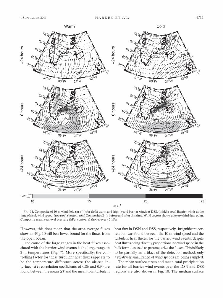
FIG. 11. Composite of 10-m wind field (m s21) for (left) warm and (right) cold barrier winds at DSS. (middle row) Barrier winds at the

time of peak wind speed. (top row),(bottom row) Composites 24 h before and after this time. Wind vectors shown at every third data point.

Composite mean sea level pressure (hPa, contours) shown every 2 hPa.


stress for both locations is about 0.8 N m22, but more

than a quarter of the events experience mean stresses of

more than 1 N m22. The precipitation rate associated

with barrier wind events is generally less at DSN than at

DSS, with median values of 0.3 and 0.7 mm h21, re-

spectively. The reduced precipitation at DSN could be in

part due to the more frequent ice cover at this location,

reducing the moisture content of the air, and the smaller

amount of uplift due to the lower topography. The range

is also greater at DSS, the warmer location.

7. Warm and cold barrier winds

To examine the synoptic conditions that bring about

the range of 2-m temperatures and hence heat fluxes,

composites of warm and cold barrier winds were pro-

duced. There is a continuous spectrum of temperatures

at both DSN and DSS (as seen via scatterplots e.g., not

shown), so an obvious criterion for distinguishing two

classes of barrier winds from temperature does not pres-

ent itself. Instead, we will take the extreme quartiles of

the 2-m temperature time series to classify warm and cold

barrier wind events and illustrate these via composites.

Each composite at DSN (DSS) contains 73 (63) events.

a. Structure

Warm barrier winds at DSS (Fig. 11, middle panels)

are characterized by a composite low pressure center

nearer to Cape Farewell than average (Fig. 8). The po-

sition of the composite cyclone channels air from the

south into a band of southeasterly winds (greater than

10 m s21) to the west of Iceland and into the barrier

wind, which is as strong as (but more localized than) the

average situation in Fig. 8.

In contrast, cold barrier winds at DSS have a com-

posite low pressure center that is located farther north-

east, closer to Iceland, and is 2 hPa deeper. This location

appears to restrict the band of southeasterly winds seen

in the warm composite and instead favors the channeling

of air from the north through the Denmark Strait and

into a long barrier wind that extends almost the entire

length of southeast Greenland (from DSN to DSS). The

maximum wind speeds are also greater than both the

warm and the total mean composites. It is worth noting

that the 2 March 2007 GFDex case of Petersen et al.

(2009) appears to be a clear example of a cold barrier

wind at DSS—in terms of the synoptic situation, barrier

flow structure, and observed temperatures.

The corresponding zero lag figures for DSN are very

similar to those for DSS in all but location of activity

(Fig. 12). In the warm class, the composite cyclone is to

the west of Iceland in a similar position to the cold DSS

composite but with a rather zonal major axis, so with

significant southerly flow. In the cold class, the composite

low is over Iceland and has a more southwest–northeast

tilt, channeling (cold) air through the Denmark Strait.

The 6 March 2007 GFDex case of Petersen et al. (2009)

appears to be a clear example of a cold barrier wind

at DSN. Similarities between the DSN and DSS events

persist throughout the subsequent analysis, so for brevity

only barrier winds at DSS will be considered from now

on. It should be presumed that results are transferable to

DSN through a translation of about 500 km northeast-

ward along the Greenland coast.

Figure 11 also shows the temporal evolution of warm

and cold barrier winds at DSS, which highlights further

differences between the classifications. For warm barrier

winds, the composite parent cyclone is located south of

FIG. 12. Composite of 10-m wind field (m s21) for (left) warm and (right) cold barrier winds detected at DSN at zero lag time in DJF of

the ERA-Interim dataset between 1989 and 2008. Wind vectors shown at every third data point. Composite mean sea level pressure (hPa,

contours) shown every 2 hPa. Wind speed color bar as in Fig. 11.


Cape Farewell 24 h previously, before moving into the

lee of Greenland for the time of the peak barrier wind,

and then appearing to become ‘‘captured’’ by Greenland—

moving no farther eastward over the next 24 h. The lee

of Greenland has been shown to be a region of cyclolysis

(Petersen et al. 2003; Hoskins and Hodges 2002). The

spreading isobars at the northeast part of the domain

suggest this is not always the case and that some cyclones

do move through the region.

For cold barrier winds, the parent cyclone begins

just east of Cape Farewell and moves progressively

northeastward throughout the 48 h. The elongation and

filling of the mean sea level pressure field at 124 h is

symptomatic of a range of translation speeds of the cy-

clones responsible for cold barrier winds. The cold

barrier wind exists for a longer time; it is evident from

224 to 124 h, initially located at DSS and then at DSN,

in agreement with the calculated phase lags (Fig. 6). In

contrast, for the warm class, the barrier winds have

a shorter life time.

The differing behavior of the surface lows can be

explained in part through analyses at 500 hPa (Fig. 13).

Warm barrier winds have strong cross-barrier flow

(18 m s21) above mountain height, associated with a well-

defined trough over the Labrador Sea and a ridge ex-

tending from the United Kingdom to east Greenland.

This upper-level flow pattern would help confine a sur-

face low to the Greenland coast and restrict its passage

through the region. It will also assist in advecting warm air

from the south toward DSS, resulting in barrier winds

with warm cores.

For cold barrier winds, the upper-level trough is lo-

cated farther east, over the west Irminger Sea, and the

ridge over the United Kingdom is shallower (Fig. 13).

The result is a weaker cross-barrier flow at 500 hPa; the

upper-level winds are orientated more zonally and far-

ther to the south, aiding the surface cyclones in passing

through the region.

The composite 2-m temperature anomalies for the

warm and cold cases are shown in Fig. 14. In the warm

composite, the region is flooded with air warmer than

the climatological mean (Fig. 3) by as much as 3 K over

the ocean and 7 K over land, the result of both the low-

level flow pattern and the strong cross-mountain flow at

500 hPa. This anomalously warm region extends from

DSS both northwest and southeast, indicative of warm

advection from the southeast and is in agreement with

the strong southeasterlies both over sea and land in

Fig. 11.

FIG. 13. Composite of 500-hPa wind field (m s21, colors) for

(top) warm and (bottom) cold barrier winds detected at DSS for

the winter months. Composite geopotential height (m, thick con-

tours) shown every 50 m and 850–1000-hPa thickness (m, thin

contours) shown every 10 m. Note larger domain of this figure.

FIG. 14. Composite of 2-m temperature anomaly (K, contours every 1 K) for (left) warm and (right) cold barrier

winds detected at DSS at zero lag time. Positive (negative) values shown with black (gray) lines.


The cold composite is characterized by an anoma-

lously cold pool of 24 K to the north of Iceland, with

a tongue extending southward through the Denmark

Strait to DSS. The shape of the cold anomaly, in con-

junction with the cold dome of air in 10002850-hPa

thickness along the east coast of Greenland (Fig. 13) and

the long barrier wind seen in Fig. 11, is consistent with

cold-air advection into the barrier wind from the north-

east. These features of warm and cold barrier winds are

corroborated by the 10002850-hPa thickness composites

(Fig. 13) but are much less obvious in the 10002500-hPa

thickness composites (not shown), indicative of these

features existing below mountain height.

Our interpretation of this analysis is that warm barrier

winds source their air from the southerly advected warm

pool, whereas even though the cold barrier winds have

milder air advected toward them, they are fed by an even

colder source of air, that is, a source northeast of the

Denmark Strait. It appears that the cold barrier winds in

particular have an offshore (i.e., downslope) contribution

(see Fig. 11). At this stage it is not possible to say whether

this minor contribution is simply a downslope deflection

of maritime air or is a downslope density-driven (kata-

batic) flow of continental air.

These configurations are reminiscent of the classical

and hybrid barrier winds along the coast of Alaska, de-

scribed in Loescher et al. (2006) and Olson and Colle

(2009). Our warm barrier winds are similar to their

classical barrier winds that form due to the coastal de-

flection of onshore winds, whereas our cold barrier

winds have similarities to their hybrid barrier winds that

have an offshore gap flow component that turns to be-

come coast parallel as it reaches the ocean. Hybrid

barrier winds are colder than classical barrier winds

because they source their air from an inshore cold

pool and the onshore synoptic flow is advected over the

cold core of the barrier wind. This is analogous to the

maritime southeasterly flow being lifted over the cold

Arctic flow seen in our cold barrier winds (see also

Petersen et al. 2009, p. 1965). Apart from these structural

FIG. 15. Composite of the mean sea level pressure anomaly (hPa, contours every 1 hPa) for (left) warm and (right)

cold barrier winds—at lag times of 248, 0, and 148 h—detected at DSS in the winter months. Positive (negative)

anomalies shown with black (gray) lines. Only values that are statistically significant at the 95% level are shown. Note

the larger domain used.


similarities though, it is unclear at this stage how similar

the dynamics of barrier winds around Greenland are to

those found off Alaska—this is left to further inves-

tigation.

Returning to the mean sea level pressure composites

(Fig. 11), it is apparent that there is not a great deal of

difference in the strength or location of the parent cy-

clone for the two classes of barrier wind events (at zero

lag). What is it about the synoptic environment then that

brings about such different local conditions? Figure 15

shows the composite mean sea level pressure anomaly

for warm and cold barrier winds at the time of peak

winds at DSS and 48 h before and after. Only points that

are statistically significant at the 95% level are shown.

For the warm class, there is a significant high pressure

anomaly of, at its peak, 10 hPa located over the Nordic

seas for the 96 h shown. This not only blocks the passage

of the low responsible for the barrier wind but also acts

to restrict cold, northerly flow along the east coast of

Greenland. This configuration therefore favors warm

advection from the south into the barrier winds. The fact

that this anomalous high pressure can be found in

a similar region throughout the 96-h period shown is

indicative of North Atlantic blocking (Rex 1950; Pelly

and Hoskins 2003) being important in the production

of warm barrier winds. The blocking high at the surface

at zero lag is consistent with the ridge at 500 hPa seen

in Fig. 13.

In contrast, the cold class is characterized by an

anomalous low pressure system of 210 hPa over the

Norwegian Sea 48 h before the peak barrier winds. This

likely represents the signature from a previous cyclone

that moved through the region and in so doing chan-

neled cold air down the east coast of Greenland. As

the cyclone responsible for the barrier wind moves into

the region, it is steered by the upper-level zonal flow

(Fig. 13) and can channel this preconditioned cold air

into a barrier wind. Forty-eight hours later, the cyclone

has exited the region to the northeast. The fact that the

pressure anomaly fields at lag times of 648 h are com-

parable suggests that this process may be repeated,

providing a ‘‘conveyor belt’’ for channeling cold air from

the Arctic down the southeastern coast of Greenland.

This ‘‘train’’ of cyclones is reminiscent of the positive

phase of the NAO. It is therefore unsurprising that the

monthly frequency of cold barrier winds correlates (in

a similar fashion to Fig. 5) with the monthly NAO index

with a correlation coefficient of 0.35. Cold events at

DSN see a similar correlation of 0.39. The warm barrier

winds are produced by blocking highs; consequently,

there is insignificant correlation between their monthly

frequency and the NAO index at both locations.

b. Impact

The impact of these different temperature regimes

can be seen in composites of the surface turbulent heat

flux for the warm and cold barrier wind classes (Fig. 16).

The cold class has a heat flux pattern that mirrors that of

the wind speed composite. Total turbulent heat fluxes of

more than 200 W m22 are seen all the way down the

southeastern coast of Greenland with bullets of nearly

400 W m22 at, and upstream of, the DSS site. The

largest heat fluxes are farther offshore than the wind

speed maximum because of the influence of near-shore

sea ice and a higher sea surface temperatures offshore.

In the warm composite, only a small signature of scarcely

more than 100 W m22 is observed at the location of

strongest winds. At all other places up the Greenland

coast, the total heat flux is less than 100 W m22. The

two temperature regimes will therefore have very dif-

ferent impacts on the ocean. This is also true for the

surface momentum flux (not shown), which is similar to

FIG. 16. Composite of total surface turbulent heat flux (W m22) for (left) warm and (right) cold barrier winds

detected at DSS at zero lag time.


the wind speed pattern (Fig. 11) and thus quite different

for the warm and cold classes. In short, the specific

synoptic environment in which Greenland barrier winds

form is vital in determining the range and spatial dis-

tribution of both surface heat and momentum fluxes

along the coast.

8. Conclusions

This climatology of barrier winds along the south-

eastern coast of Greenland has confirmed (see MR05)

that there are two predominant regions where barrier

winds frequently occur—referred to as Denmark Strait

North (DSN) and South (DSS). During the 20 yr of the

climatology, barrier winds stronger than 20 m s21 occur

at both locations on average once a week in the winter

months (DJF).

Good correlations were found between the monthly

frequency of barrier winds and the monthly NAO in-

dex (especially at DSN). The relationship is explained

in the following way. A high NAO index is the result of

stronger and more frequent cyclones through the re-

gion, which are likely to trigger more and stronger

barrier winds. It is possible that this correlation will

potentially allow for the reconstruction of barrier wind

frequency for periods of time before reanalysis are

available.

One of the most striking features of the barrier winds

investigated was the large range in 2-m temperatures—

southeast Greenland barrier winds cannot be said to be

typically cold or warm winds. An investigation into the

meteorological conditions responsible for the warmest

and coldest barrier winds showed that blocking highs are

responsible for channeling warm air into warm barrier

winds and that trains of cyclones can consecutively channel

cold air down the east coast of Greenland and into cold

barrier winds. A very different pattern in the surface heat

and momentum fluxes is seen for each temperature re-

gime, and this shows the importance of the wider mete-

orological environment in understanding the local wind

forcing in the region.

Acknowledgments. We thank the following people

and organizations: The European Centre for Medium-

Range Weather Forecasts and the British Atmospheric

Data Centre for providing the data; Bob Pickart for

accommodating the launching of radiosondes on the

Knorr cruise in October 2008; NCAS FGAM for pro-

viding the radiosonde equipment; Stefan Klink and

Rudolf Krockauer from EUCOS for funding the ra-

diosondes; Hreinn Hjartson from the Icelandic Met

Office for providing equipment and assistance for ra-

diosonde launches; Geraint Vaughan and Hugo Ricketts

for radiosonde training; John Alberts and Eric Benway

of WHOI for shipping equipment; and the radiosonde

launchers for all their efforts in rough conditions.

REFERENCES

Bell, G. D., and L. F. Bosart, 1988: Appalachian cold-air damming.

Mon. Wea. Rev., 116, 137–161.

Berrisford, P., D. Dee, K. Fielding, M. Fuentes, P. Kallberg,

S. Kobayashi, and S. Uppala, 2009: The ERA-Interim archive.

ERA Rep. Series, No. 1, ECMWF, 20 pp.

Braun, S. A., R. Rotunno, and J. B. Klemp, 1999: Effects of coastal

orography on landfalling cold fronts. Part I: Dry, inviscid dy-

namics. J. Atmos. Sci., 56, 517–533.

Chen, W.-D., and R. B. Smith, 1987: Blocking and deflection of

airflow by the Alps. Mon. Wea. Rev., 115, 2578–2597.

Colle, B. A., and C. F. Mass, 1995: The structure and evolution of

cold surges east of the Rocky Mountains. Mon. Wea. Rev., 123,

2577–2610.

Cui, Z., M. Tjernstrom, and B. Grisogono, 1998: Idealized simu-

lations of atmospheric coastal flow along the central coast of

California. J. Appl. Meteor., 37, 1332–1363.

Doyle, J. D., and M. A. Shapiro, 1999: Flow response to large-scale

topography: The Greenland tip jet. Tellus, 51A, 728–748.

Ebuchi, N., H. C. Graber, and M. J. Caruso, 2002: Evaluation of

wind vectors observed by QuikSCAT/SeaWinds using ocean

buoy data. J. Atmos. Oceanic Technol., 19, 2049–2062.

Haine, T. W. N., S. Zhang, G. W. K. Moore, and I. A. Renfrew,

2009: On the impact of high-resolution, high-frequency me-

teorological forcing on Denmark Strait ocean circulation.

Quart. J. Roy. Meteor. Soc., 135, 2067–2085.

Heinemann, G., and T. Klein, 2002: Modelling and observations

of the katabatic flow dynamics over Greenland. Tellus, 54A,

542–554.

Hoskins, B. J., and K. I. Hodges, 2002: New perspectives on the

Northern Hemisphere winter storm tracks. J. Atmos. Sci., 59,

1041–1061.

Hurrell, J. W., 1995: Decadal trends in the North Atlantic Oscil-

lation: Regional temperatures and precipitation. Science, 269,

676–679.

Klein, T., and G. Heinemann, 2002: Interaction of katabatic winds

and mesocyclones near the eastern coast of Greenland. Meteor.

Appl., 9, 407–422.

Kristjansson, J. E., and H. McInnes, 1999: The impact of Greenland

on cyclone evolution in the North Atlantic. Quart. J. Roy.

Meteor. Soc., 125, 2819–2834.

Loescher, K. A., G. S. Young, B. A. Colle, and N. S. Winstead, 2006:

Climatology of barrier jets along the Alaskan coast. Part I: Spatial

and temporal distributions. Mon. Wea. Rev., 134, 437–453.

Martin, R., and G. W. K. Moore, 2006: Transition of a synoptic

system to a polar low via interaction with the orography of

Greenland. Tellus, 58A, 236–253.

Moore, G. W. K., 2003: Gale force winds over the Irminger Sea to

the east of Cape Farewell, Greenland. Geophys. Res. Lett., 30,

1894, doi:10.1029/2003GL018012.

——, and I. A. Renfrew, 2005: Tip jets and barrier winds: A

QuikSCAT climatology of high wind speed events around

Greenland. J. Climate, 18, 3713–3725.

——, R. S. Pickart, and I. A. Renfrew, 2008: Buoy observations

from the windiest location in the world ocean, Cape Farewell,

Greenland. Geophys. Res. Lett., 35, L18802, doi:10.1029/

2008GL034845.


Olson, J. B., and B. A. Colle, 2009: Three-dimensional idealized

simulations of barrier jets along the southeast coast of Alaska.

Mon. Wea. Rev., 137, 391–413.

Outten, S. D., I. A. Renfrew, and G. N. Petersen, 2009: An easterly

tip jet off Cape Farewell, Greenland. II: Simulations and dy-

namics. Quart. J. Roy. Meteor. Soc., 135, 1934–1949.

——, ——, and ——, 2010: Erratum: An easterly tip jet off Cape

Farewell, Greenland. II: Simulations and dynamics. Quart.

J. Roy. Meteor. Soc., 136, 1099–1101.

Parish, T. R., 1982: Barrier winds along the Sierra Nevada Moun-

tains. J. Appl. Meteor., 21, 925–930.

——, 1983: The influence of the Antarctic Peninsula on the wind

field over the western Weddell Sea. J. Geophys. Res., 88, 2684–

2692.

Pelly, J. L., and B. J. Hoskins, 2003: A new perspective on blocking.

J. Atmos. Sci., 60, 743–755.

Petersen, G. N., H. Olafsson, and J. E. Kristjansson, 2003: Flow in

the lee of idealized mountains and Greenland. J. Atmos. Sci.,

60, 2183–2195.

——, J. E. Kristjansson, and H. Olafsson, 2005: The effect of up-

stream wind direction on atmospheric flow in the vicinity of

a large mountain. Quart. J. Roy. Meteor. Soc., 131, 1113–1128.

——, I. A. Renfrew, and G. W. K. Moore, 2009: An overview of

barrier winds off southeastern Greenland during the Greenland

Flow Distortion Experiment. Quart. J. Roy. Meteor. Soc., 135,

1950–1967.

Pickart, R. S., M. A. Spall, M. H. Ribergaard, G. W. K. Moore, and

R. F. Milliff, 2003: Deep convection in the Irminger Sea forced

by the Greenland tip jet. Nature, 424, 152–156.

Pierrehumbert, R. T., and B. Wyman, 1985: Upstream effects of

mesoscale mountains. J. Atmos. Sci., 42, 977–1003.

Rabier, F., J.-N. Thepaut, and P. Courtier, 1998: Extended assim-

ilation and forecast experiments with a four-dimensional

variational assimilation system. Quart. J. Roy. Meteor. Soc.,

124, 1861–1887.

Renfrew, I. A., G. W. K. Moore, P. S. Guest, and K. Bumke, 2002:

A comparison of surface layer and surface turbulent flux ob-

servations over the Labrador Sea with ECMWF analyses and

NCEP reanalyses. J. Phys. Oceanogr., 32, 383–400.

——, and Coauthors, 2008: The Greenland Flow Distortion Ex-

periment. Bull. Amer. Meteor. Soc., 89, 1307–1324.

——, S. D. Outten, and G. W. K. Moore, 2009a: An easterly tip jet

off Cape Farewell, Greenland. I: Aircraft observations. Quart.

J. Roy. Meteor. Soc., 135, 1919–1933.

——, G. N. Petersen, D. A. J. Sproson, G. W. K. Moore, H. Adiwidjaja,

S. Zhang, and R. North, 2009b: A comparison of aircraft-based

surface-layer observations over Denmark Strait and the Ir-

minger Sea with meteorological analyses and QuikSCAT

winds. Quart. J. Roy. Meteor. Soc., 135, 2046–2066.

Revell, M. J., J. H. Copeland, H. R. Larsen, and D. S. Wratt, 2002:

Barrier jets around the southern Alps of New Zealand and their

potential to enhance alpine rainfall. Atmos. Res., 61, 277–298.

Rex, D. F., 1950: Blocking action in the middle troposphere and its

effect upon regional climate. I. An aerological study of

blocking action. Tellus, 2, 196–211.

Sahsamanoglou, H. S., 1990: A contribution to the study of

action centres in the North Atlantic. Int. J. Climatol., 10,

247–261.

Sampe, T., and S.-P. Xie, 2007: Mapping high sea winds from space:

A global climatology. Bull. Amer. Meteor. Soc., 88, 1965–1978.

Schwerdtfeger, W., 1975: The effect of the Antarctic Peninsula on

the temperature regime of the Weddell Sea. Mon. Wea. Rev.,

103, 45–51.

Serreze, M. C., F. Carse, R. G. Barry, and J. C. Rogers, 1997:

Icelandic low cyclone activity: Climatological features, linkages

with the NAO, and relationships with recent changes in the

Northern Hemisphere circulation. J. Climate, 10, 453–464.

Skeie, R. B., J. E. Kristjansson, H. Olafsson, and B. Røsting, 2006:

Dynamical processes related to cyclone development near

Greenland. Meteor. Z., 15, 147–156.

Smith, S. D., 1988: Coefficients for sea surface wind stress, heat flux,

and wind profiles as a function of wind speed and temperature.

J. Geophys. Res., 93, 15 467–15 472.

Sproson, D. A. J., I. A. Renfrew, and K. J. Heywood, 2008: At-

mospheric conditions associated with oceanic convection in

the south-east Labrador Sea. Geophys. Res. Lett., 35, L06601,

doi:10.1029/2007GL032971.

Straneo, F., G. S. Hamilton, D. A. Sutherland, L. A. Stearns,

F. Davidson, M. O. Hammill, G. B. Stenson, and A. Rosing-

Asvid, 2010: Rapid circulation of warm subtropical waters in

a major glacial fjord in east Greenland. Nat. Geosci., 3, 182–186.

Vage, K., R. S. Pickart, G. W. K. Moore, and M. H. Ribergaard,

2008: Winter mixed layer development in the central Irminger

Sea: The effect of strong, intermittent wind events. J. Phys.

Oceanogr., 38, 541–565.

——, T. Spengler, H. C. Davies, and R. S. Pickart, 2009: Multi-event

analysis of the westerly Greenland tip jet based upon 45 winters

in ERA-40. Quart. J. Roy. Meteor. Soc., 135, 1999–2011.


Documents

A Climatology of Wintertime Barrier Winds off Southeast