A class of Recursive Permutationswhich is Primitive Recursive complete

Luca Paolinia, Mauro Piccoloa, Luca Roversia

aDipartimento di Informatica – Universita di Torino

Abstract

We focus on total functions in the theory of reversible computational mod-els. We define a class of recursive permutations, dubbed Reversible PrimitivePermutations (RPP) which are computable invertible total endo-functions onintegers, so a subset of total reversible computations. RPP is generated fromfive basic functions (identity, negation, successor, predecessor, swap), two no-tions of composition (sequential and parallel), one functional iteration and onefunctional selection. Also, RPP is closed by inversion, is expressive enough toencode Cantor pairing and the whole class of Primitive Recursive Functions.

Keywords: Reversible Computation, Unconventional Computing Models,Computable Permutations.PACS: code, codePACS:

1. Introduction

Mainstream computer science tends to see models of computations as toolsthat strongly focus on one of the two possible directions of computation. Wetypically think how to model the way the computation evolves from inputs tooutputs while we (reasonably) overlook the behavior in the opposite direction,from outputs to inputs. Thus, in general, models of computations are not back-ward deterministic (and not reversible.)

For a very rough intuition about what reversible computation deals with, westart by an example. Let us think about our favorite programming languageand think of implementing the addition between two natural numbers m andn. Very likely — of course without absolute certainty — we shall end up withsome procedure sum which takes two arguments and which yields their sum. For

Email addresses: paolini@di.unito.it, luca.paolini@unito.it (Luca Paolini),piccolo@di.unito.it, mauro.piccolo@unito.it (Mauro Piccolo), roversi@di.unito.it,luca.roversi@unito.it (Luca Roversi)

URL: http://www.di.unito.it/~paolini (Luca Paolini),http://www.di.unito.it/~piccolo (Mauro Piccolo), http://www.di.unito.it/~rover(Luca Roversi)

Preprint submitted to Elsevier February 21, 2017

example, sum(3,2) would yield 5. What if we think of asking for the values mand n such that sum(m,n) = 5? If we had implemented sum in a prolog-likelanguage, then we could exploit its non deterministic evaluation mechanism tolist all the pairs (0, 5), (1, 4), (2, 3), (3, 2), (4, 1) and (5, 0) all of which would wellbe a correct instance of (m,n). In a reversible setting we would obtain exactlythe pair we started from. I.e., the computation would be backward determinis-tic. The interest for the backward determinism arose in the sixties of the lastcentury, studying the thermodynamics of computation and the connections be-tween information theory, computability and entropy. After then, the interestfor the reversible computing has slowly but incessantly grown.

Here, some general non-exhaustive list of references follows. Reversible Tur-ing machines are in [19, 2] and [1, 10] study some of their computational theoreticproperties. Many research efforts have been focused on boolean functions andcellular automata as models of the reversible computation (see [25, 36] for in-stance.) Moreover, some research focused on reversible programming languages,like [11, 37]. Of course the interest to build a comprehensive knowledge aboutreversible computation is much wider than the (“mere”) will to fully cover itscomputational theoretic aspects. The book [28] is a comprehensive introductionto the subject which spans from low-power-consumption reversible hardware toemerging alternative computational models like quantum [7, 38] or bio-inspired[6] of which reversibility is one the unavoidable building blocks.

Goal. The focus of this work is on a functional model of reversible computation.Specifically, we look for a sufficiently expressive class of recursive permutationsable to represent all Dedekind-Rozsa-Robinson’s Primitive Recursive Functions(PRF) [30, 34] whose relevance can be traced to the slogan “programs whichterminate but do not belong to PRF are rarely of practical interest”.

In analogy to PRF, we aim at getting a functional characterization of com-putability and proof theoretical notions – but in a reversible setting, of course— because functions are handier to compose algorithms than other models like,for example, Turing machines-oriented models which, instead, are much moreconvincing from the implementation view-point. The main key point of PRFthat the functional characterization we are looking for must include is the pos-sibility of representing Cantor pairing [31] which means the ability to expressall interesting total properties about the traces of Turing machines and of Re-versible Turing machines. Last but not least, such a functional characterizationmust be closed under inversion, which is a very natural to ask for in a class ofpermutations and of reversible computing models.

Our quest is challenging because various negative results could have pre-vented success. First of all, we remark that the class of all (total) recursivepermutations cannot be finitely effectively enumerated (see [30, Exercise 4-6,p.55]). Since all recursive permutations can be constructively generated start-ing from the set of primitive recursive permutations [13], it follows that alsothe primitive recursive permutations cannot be enumerated. Worst, the prim-itive recursive permutations are not closed by inversion, as proved in [15] (see[27, 34]). For sake of completeness, we recall that similar negative results holds

2

also for elementary permutations: they cannot be effectively enumerated andthey are not closed by inversion (see [4, 12, 14]). Summing up, no hope existsto find any (effective) description neither of the class of recursive permutationsnor of the classes of primitive recursive permutations and of elementary permu-tations.

Literature Comparison. Our quest on the identification of the reversible analo-gous of PRF must be throughly related to the following works.

• Armando Matos [21] proposes variants of a programming language inspiredto LOOP programs (i.e. programs of a language that Meyer and Ritchie[24] conceived to program PRF functions.) Matos is the first researcherwho adopts Z as ground data for his analysis. We share the choice withhim. The work [21] focuses on the algebraic aspects of his languagesand his relations with group of matrices. Matos leaves the comparisonbetween “the classes of SRL- and ESRL-definable functions with the classof primitive recursive functions” as future work. Also, unpublished notesby Matos exist [22]. They extend his published works by showing that*-SRL is sufficiently expressive to simulate reversible circuits [36] and thatPRF-functions contain *-SRL via a suitable embedding. *-SRL is quiteclose to the class RPP we propose. Nevertheless, we conjecture that novariant of Matos’ languages exists able to simulate the functional selectionwe have in RPP.

• [27] is a precursor of this work which we improve in at least two respects.[27] introduces the class RPRF which is closed by inversion and is PRF-complete. The main difference between RPRF and the class RPP we intro-duce here is that the definition of the latter is strictly more essential thanthe definition of the former. Specifically, Section 5 shows how to repre-sent Cantor pairing in RPP which is the key to encode stacks of integersinside RPP and to obtain its PRF-completeness as in Section 6. Instead,the encoding of stacks inside RPRF relies on primitives which pair andunpair integers — in analogy to Cantor pairing —, but which we explicitlyincluded in the definition of RPRF. Therefore, we here indirectly provethat RPRF in [27] contains (unnecessary) syntactic sugar.

Both in [27] and in this work the PRF-completeness of RPRF and RPPrelies on ancillary arguments. However, the map from PRF and RPP wepropose here fully internalizes what is known as Bennett’s trick. Thismeans leaving ancillae without any garbage in them, at the end of thesimulation of any f ∈ PRF as a function of RPP. This is not true for thesimulation of f ∈ PRF as an element of RPRF. Technically, the difference isevident by comparing Definition 3 of Section 6 which fixes how to representany f ∈ PRF into RPP and the corresponding definition in [27].

• Finally we focus on [9]. It introduces the class of reversible functionsRI which is as expressive as Kleene partial recursive functions [5, 26].Therefore, the focus of [9] is on partial reversible functions while ours is

3

on total ones. The expressiveness of RI is clearly stronger than the one ofRPP. However, we see RI as less abstract than RPP for two reasons. Onone side, the primitive functions of RI relies on the given specific binaryrepresentation of natural numbers. On the other, it is not evident thatRI is the extension of a total sub-class analogous to RPP which shouldideally correspond to PRF, but in a reversible setting.

Contributions. We propose a formalism that identifies a class of functions whichwe call Reversible Primitive Permutations (RPP) and which is strictly includedin the set of total invertible functions.

Section 2 defines RPP in analogy with the definition of PRF, i.e. RPP is theclosure of composition schemes on basic functions.

The functions of RPP have identical arity and co-arity and take Z — andnot only N — as their domain because N is not a group. So, RPP is sufficientlyabstract to avoid any reference to any specific encoding of numbers and stronglyconnects our work to Matos’ one [21].

For example, in RPP we can define a sum that given the two integers m andn yields m+ n and n. Let us represent sum as:

mn

[sum

]m + nn . (1)

The implementation of sum inside RPP exploits an iteration scheme that iteratesn times the successor, starting on the initial value m of the first input. RPPimplies the existence of a (meta and) effective procedure which produces theinverse f−1 ∈ RPP of every given f ∈ RPP. I.e., :

pn

[sum−1

]p− nn (2)

belongs to RPP and it “undoes” sum by iterating n times the predecessor on p.So if p = m + n, then p − n = m + n − n = m. We remark we could haveinternalized the operation that yields the inverse of a function inside RPP likein [21]. We choose not for sake of simplicity, so avoiding mutually recursivedefinitions inside RPP.

Concerning the expressiveness, RPP is both PRF-complete and PRF-sound.Completeness is the really relevant property between the two because this meansthat RPP subsumes the class PRF. This result is in Section 6. It requires quitea lot of preliminary work that one can find in Sections 3, 4 and 5 and whosegoal is to encode a bounded minimalization, Cantor pairing and the stack asdata-type. So, the embedding makes evident various key aspects of reversiblecomputing. The principal ones we like to underline are how to encode Cantorpairing, the unavoidable use of ancillary variables to clone information and thecompositional programming under the pattern that Bennett’s trick dictates (cf.Section 7.)

Concerning RPP-soundness, which means that PRF subsumes RPP, we ad-dress the reader to [27] as a possible reference to the obvious idea about howformally defining an embedding from RPP into PRF.

4

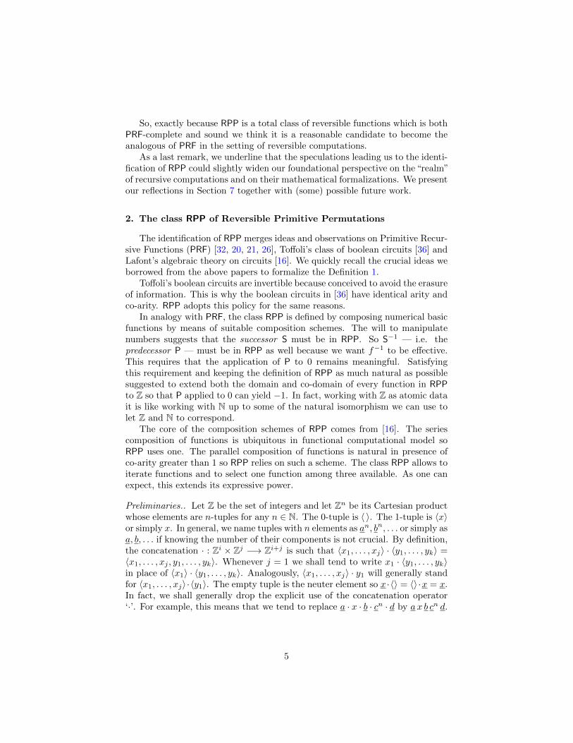
So, exactly because RPP is a total class of reversible functions which is bothPRF-complete and sound we think it is a reasonable candidate to become theanalogous of PRF in the setting of reversible computations.

As a last remark, we underline that the speculations leading us to the identi-fication of RPP could slightly widen our foundational perspective on the “realm”of recursive computations and on their mathematical formalizations. We presentour reflections in Section 7 together with (some) possible future work.

2. The class RPP of Reversible Primitive Permutations

The identification of RPP merges ideas and observations on Primitive Recur-sive Functions (PRF) [32, 20, 21, 26], Toffoli’s class of boolean circuits [36] andLafont’s algebraic theory on circuits [16]. We quickly recall the crucial ideas weborrowed from the above papers to formalize the Definition 1.

Toffoli’s boolean circuits are invertible because conceived to avoid the erasureof information. This is why the boolean circuits in [36] have identical arity andco-arity. RPP adopts this policy for the same reasons.

In analogy with PRF, the class RPP is defined by composing numerical basicfunctions by means of suitable composition schemes. The will to manipulatenumbers suggests that the successor S must be in RPP. So S−1 — i.e. thepredecessor P — must be in RPP as well because we want f−1 to be effective.This requires that the application of P to 0 remains meaningful. Satisfyingthis requirement and keeping the definition of RPP as much natural as possiblesuggested to extend both the domain and co-domain of every function in RPPto Z so that P applied to 0 can yield −1. In fact, working with Z as atomic datait is like working with N up to some of the natural isomorphism we can use tolet Z and N to correspond.

The core of the composition schemes of RPP comes from [16]. The seriescomposition of functions is ubiquitous in functional computational model soRPP uses one. The parallel composition of functions is natural in presence ofco-arity greater than 1 so RPP relies on such a scheme. The class RPP allows toiterate functions and to select one function among three available. As one canexpect, this extends its expressive power.

Preliminaries.. Let Z be the set of integers and let Zn be its Cartesian productwhose elements are n-tuples for any n ∈ N. The 0-tuple is 〈 〉. The 1-tuple is 〈x〉or simply x. In general, we name tuples with n elements as an, bn, . . . or simply asa, b, . . . if knowing the number of their components is not crucial. By definition,the concatenation · : Zi × Zj −→ Zi+j is such that 〈x1, . . . , xj〉 · 〈y1, . . . , yk〉 =〈x1, . . . , xj , y1, . . . , yk〉. Whenever j = 1 we shall tend to write x1 · 〈y1, . . . , yk〉in place of 〈x1〉 · 〈y1, . . . , yk〉. Analogously, 〈x1, . . . , xj〉 · y1 will generally standfor 〈x1, . . . , xj〉 ·〈y1〉. The empty tuple is the neuter element so x · 〈〉 = 〈〉 ·x = x.In fact, we shall generally drop the explicit use of the concatenation operator‘·’. For example, this means that we tend to replace a · x · b · cn · d by a x b cn d.

5

Definition 1 (Reversible Primitive Permutations). Reversible PrimitivePermutations (abbreviates as RPP) is a sub-class of Reversible Permutations1.By definition, RPP =

⋃k∈N RPPk where, for every k ∈ N, the set RPPk contains

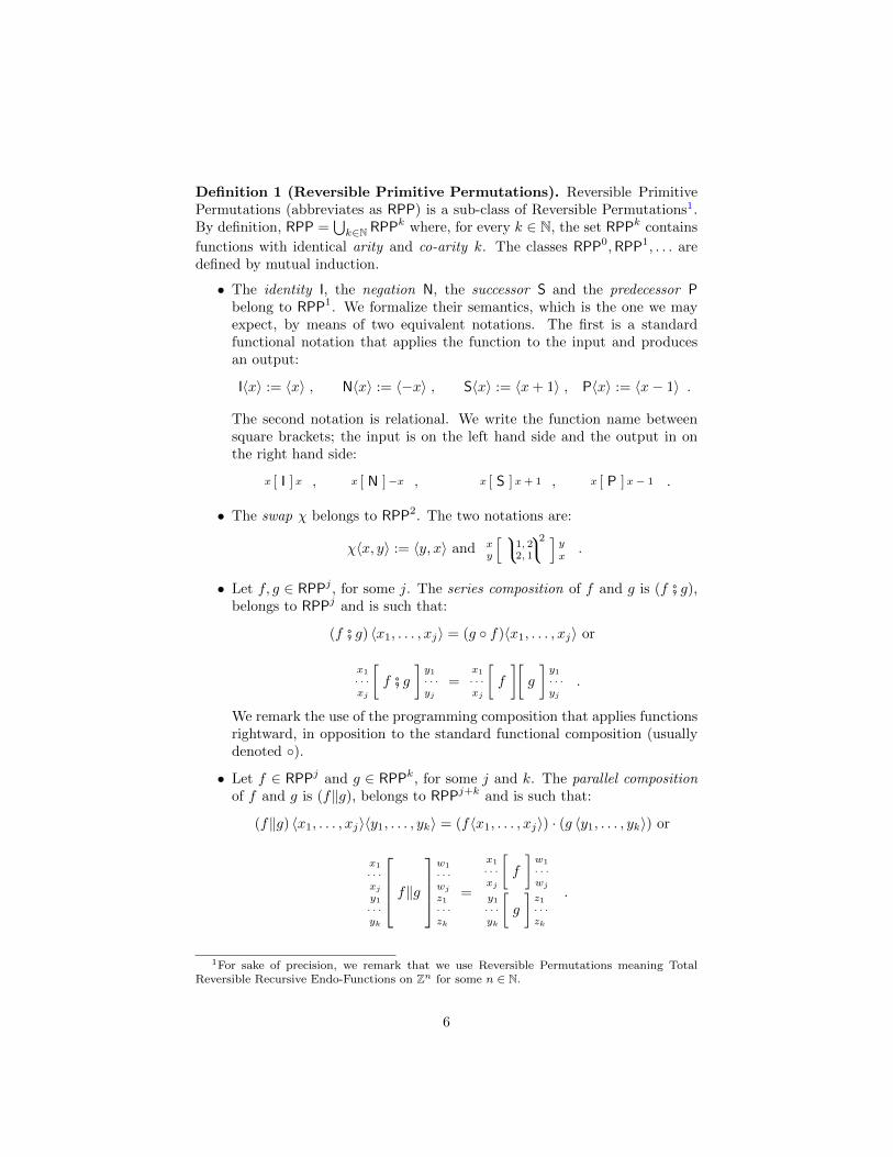
functions with identical arity and co-arity k. The classes RPP0,RPP1, . . . aredefined by mutual induction.

• The identity I, the negation N, the successor S and the predecessor Pbelong to RPP1. We formalize their semantics, which is the one we mayexpect, by means of two equivalent notations. The first is a standardfunctional notation that applies the function to the input and producesan output:

I〈x〉 := 〈x〉 , N〈x〉 := 〈−x〉 , S〈x〉 := 〈x+ 1〉 , P〈x〉 := 〈x− 1〉 .

The second notation is relational. We write the function name betweensquare brackets; the input is on the left hand side and the output in onthe right hand side:

x [ I ] x , x [ N ]−x , x [ S ] x + 1 , x [ P ] x− 1 .

• The swap χ belongs to RPP2. The two notations are:

χ〈x, y〉 := 〈y, x〉 and xy

[ 1, 22, 1

2 ]y

x.

• Let f, g ∈ RPPj , for some j. The series composition of f and g is (f # g),belongs to RPPj and is such that:

(f # g) 〈x1, . . . , xj〉 = (g ◦ f)〈x1, . . . , xj〉 or

x1

· · ·xj

[f # g

]y1

· · ·yj

=x1

· · ·xj

[f

][g

]y1

· · ·yj

.

We remark the use of the programming composition that applies functionsrightward, in opposition to the standard functional composition (usuallydenoted ◦).

• Let f ∈ RPPj and g ∈ RPPk, for some j and k. The parallel compositionof f and g is (f‖g), belongs to RPPj+k and is such that:

(f‖g) 〈x1, . . . , xj〉〈y1, . . . , yk〉 = (f〈x1, . . . , xj〉) · (g 〈y1, . . . , yk〉) or

x1

· · ·xjy1

· · ·yk

f‖g

w1

· · ·wjz1· · ·zk

=

x1

· · ·xj

[f

]w1

· · ·wj

y1

· · ·yk

[g

]z1· · ·zk

.

1For sake of precision, we remark that we use Reversible Permutations meaning TotalReversible Recursive Endo-Functions on Zn for some n ∈ N.

6

• Let f ∈ RPPk. The finite iteration of f is It [f ], belongs to RPPk+1 andis such that:

It [f ] (〈x1, . . . , xk〉 · x) = ((

|x|︷ ︸︸ ︷f # . . . # f)‖I) (〈x1, . . . , xk〉 · x) or

x1

· · ·xk

x

It [f ]

y1

· · ·yk

= (f # . . . # f︸ ︷︷ ︸|x|

) 〈x1, . . . , xk〉

x

.

We remark the linearity constraint on the finite iteration. The argumentx which drives the iteration unfolding cannot be among the arguments ofthe iterated function f . Moreover, we choose to use x as the last argumentof It [f ] to avoid any re-indexing of the arguments of f when iterating it.

• Let f, g, h ∈ RPPk. The selection of one among f, g and h is If [f, g, h], itbelongs to RPPk+1 and is such that:

If [f, g, h] (〈x1, . . . , xk〉 · x) =

(f‖I) (〈x1, . . . , xk〉 · x) if x > 0

(g‖I) (〈x1, . . . , xk〉 · x) if x = 0

(h‖I) (〈x1, . . . , xk〉 · x) if x < 0

or

x1

· · ·xk

x

If [f, g, h]

y1

· · ·yk

=

f 〈x1, . . . , xk〉 if x > 0

g 〈x1, . . . , xk〉 if x = 0

h 〈x1, . . . , xk〉 if x < 0

x

.

We remark the linearity constraint imposed on the definition of selection.The argument x which determines which among f, g and h must be usedcannot be among the arguments of f, g and h. Moreover, we choose touse x as the last argument of If [f, g, h] to avoid any re-indexing of thearguments of f, g and h, once we choose one of them.

Proposition 1 (Finite Permutations in RPP.). Each finite permutation witharity and co-arity equal to k belongs to RPPk.

Proof. A transposition is a permutation which exchanges two elements andkeeps all others fixed. Each finite permutation is generated by compositions oftranspositions.

Notation 1. If the same value occurs in consecutive inputs or outputs, like, forexample, in:

f〈x1, . . . , xm, 0, . . . , 0︸ ︷︷ ︸r∈N

, y1, . . . , yn〉 = 〈w1, . . . , wp, 0, . . . , 0︸ ︷︷ ︸s∈N

, z1, . . . , zq〉 ,

7

with m+ r + n = p+ s+ q, we tend to abbreviate it as:

f〈x1, . . . , xm, 0r, y1, . . . , yn〉 = 〈w1, . . . , wp, 0

s, z1, . . . , zq〉 or

x1

· · ·xm

0r

y1

· · ·yn

f

w1

· · ·wp

0s

z1· · ·zq

.

In particular, 00 means that no occurrences of 0 exist.

To come up with the identification of RPP we have been looking for a reason-ably expressive class of total and numerical functions in which it is possible togive a gentle (as opposed to “brute force”2) status to the operation of inversinga given function f ; we mean that the operation f−1, which we standardly defineas the one such that (y, x) ∈ f−1 if and only if (x, y) ∈ f is effective inside RPP.

Proposition 2 (The (syntactical) inverse f−1 of any f). Let f ∈ RPPj, forany j ∈ N. The inverse of f is f−1, belongs to RPPj and, by definition, is:

I−1 := I , N−1 := N , S−1 := P , P−1 := S , χ−1 := χ ,

(g # f)−1

:= f−1 # g−1 , (f‖g)−1

:= f−1‖g−1 ,

(It [f ])−1

:= It[f−1

], (If [f, g, h])

−1:= If

[f−1, g−1, h−1

].

Then f # f−1 = I and f−1 # f = I.

Proof. By induction on the definition of f .

Proposition 3 (Relating series composition and parallel composition). Letf, g ∈ RPPj and f ′, g′ ∈ RPPk with j, k ∈ N. Then:

(f‖f ′) # (g‖g′) = (f # g)‖(f ′ # g′) .

Proof. By definition:

(f‖f ′) # (g‖g′) a b = (g‖g′)(f‖f ′) a b= (g‖g′) (fa) (f ′b)

= (gfa)(g′f ′b)

= ((f # g) a)((f ′ # g′) b)= ((f # g)‖(f ′ # g′)) a b .

As a concluding remark, we underline that, in the course of the design of RPP,we aimed at sticking as much as we could to the traditional formalism that PRFrepresents. In the mean time we tried to keep a reasonable balance betweenconciseness and easiness of usage which can become quite cumbersome becauseof the “rewiring” that finite permutations imply.

2We remark that the inversion of total recursive functions is possible by using the bruteforce, see [29, 23].

8

3. Generalizations inside RPP

We introduce formal generalizations of elements in RPP. This helps simpli-fying the use of RPP as a programming notation.

Weakening inside RPP. For any given f ∈ RPPm an infinite set {wn(f) | n ≥1 and wn(f) ∈ RPPm+n} exists such that:

x1

· · ·xm

xm+1

· · ·xm+n

wn(f)

y1

· · ·yn

= f 〈x1, . . . , xm〉

xm+1

· · ·xm+n

,

for every wn(f). We call wn(f) weakening of f which we can obviously obtainby parallel composition of f with n occurrences of I. In general, if we needsome weakening of a given f , then we shall not write wn(f) explicitly. We shallinstead use f and say that it is the weakening of f itself.

Generalized identity, negation, successor and predecessor. For every i ≤ n, thefollowing functions in RPPn exist:

In 〈x1, . . . , xi−1, xi, xi+1, . . . , xn〉 = 〈x1, . . . , xi−1, xi, xi+1, . . . , xn〉Nn

i 〈x1, . . . , xi−1, xi, xi+1, . . . , xn〉 = 〈x1, . . . , xi−1,−xi, xi+1, . . . , xn〉Sni 〈x1, . . . , xi−1, xi, xi+1, . . . , xn〉 = 〈x1, . . . , xi−1, xi + 1, xi+1, . . . , xn〉Pni 〈x1, . . . , xi−1, xi, xi+1, . . . , xn〉 = 〈x1, . . . , xi−1, xi − 1, xi+1, . . . , xn〉 .

They are the weakening of I,N,S,P ∈ RPP1. When the arity n is clear from thecontext, sometimes we shall use I,Ni,Si and Pi in place of In,Nn

i ,Sni and Pn

i .

Generalized syntactic permutations. Let {i1, . . . , in} = {1, . . . , n} and ρ : Nn −→Nn be any permutation. There is at least one definition of the following gener-alized syntactic permutation: i1 ,..., im

ρ(i1),...,ρ(im)

n , (3)

which belongs to RPPn, and which sends the i1-th input to the ρ(i1)-th output,the i2-th input to the ρ(i2)-th output etc.. No restrictions exist on the orderof i1, . . . , im. From Proposition 1, every generalized syntactic permutation isobviously a suitable composition of identity , binary syntactic permutation, seriescomposition, parallel composition and weakening .

Generalized finite iteration. Let f ∈ RPPn and m ≥ n + 1. Let 〈xi〉, L =〈xi1 , . . . , xin〉 and 〈xj1 , . . . , xjm−n−1

〉 be three lists which partition 〈x1, . . . , xm〉.

9

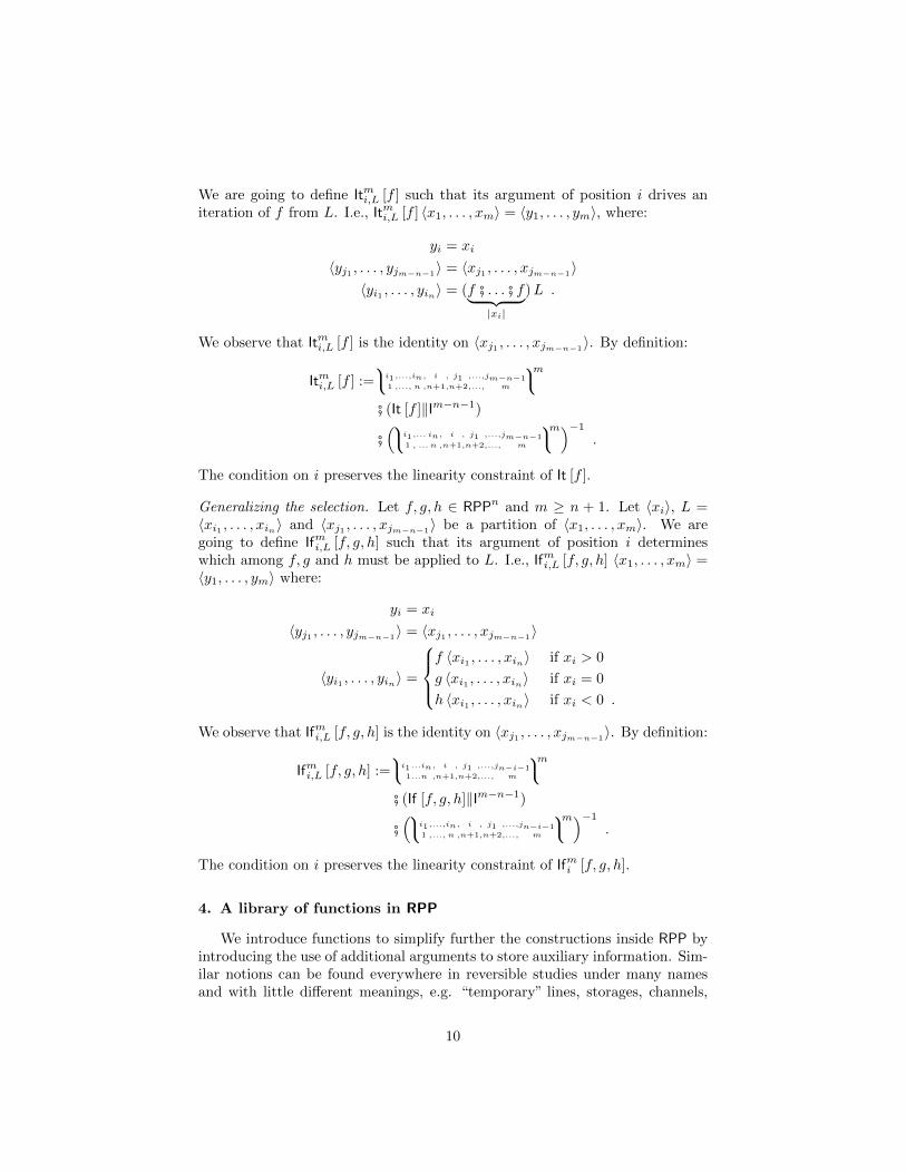
We are going to define Itmi,L [f ] such that its argument of position i drives aniteration of f from L. I.e., Itmi,L [f ] 〈x1, . . . , xm〉 = 〈y1, . . . , ym〉, where:

yi = xi

〈yj1 , . . . , yjm−n−1〉 = 〈xj1 , . . . , xjm−n−1

〉〈yi1 , . . . , yin〉 = (f # . . . # f︸ ︷︷ ︸

|xi|

)L .

We observe that Itmi,L [f ] is the identity on 〈xj1 , . . . , xjm−n−1〉. By definition:

Itmi,L [f ] :=i1,...,in, i , j1 ,...,jm−n−1

1 ,..., n ,n+1,n+2,..., m

m# (It [f ]‖Im−n−1)

#(i1,... in, i , j1 ,...,jm−n−1

1 , ... n ,n+1,n+2,..., m

m)−1

.

The condition on i preserves the linearity constraint of It [f ].

Generalizing the selection. Let f, g, h ∈ RPPn and m ≥ n + 1. Let 〈xi〉, L =〈xi1 , . . . , xin〉 and 〈xj1 , . . . , xjm−n−1

〉 be a partition of 〈x1, . . . , xm〉. We aregoing to define Ifmi,L [f, g, h] such that its argument of position i determineswhich among f, g and h must be applied to L. I.e., Ifmi,L [f, g, h] 〈x1, . . . , xm〉 =〈y1, . . . , ym〉 where:

yi = xi

〈yj1 , . . . , yjm−n−1〉 = 〈xj1 , . . . , xjm−n−1

〉

〈yi1 , . . . , yin〉 =

f 〈xi1 , . . . , xin〉 if xi > 0

g 〈xi1 , . . . , xin〉 if xi = 0

h 〈xi1 , . . . , xin〉 if xi < 0 .

We observe that Ifmi,L [f, g, h] is the identity on 〈xj1 , . . . , xjm−n−1〉. By definition:

Ifmi,L [f, g, h] :=i1...in, i , j1 ,...,jn−i−1

1...n ,n+1,n+2,..., m

m# (If [f, g, h]‖Im−n−1)

#(i1,...,in, i , j1 ,...,jn−i−1

1 ,..., n ,n+1,n+2,..., m

m)−1

.

The condition on i preserves the linearity constraint of Ifmi [f, g, h].

4. A library of functions in RPP

We introduce functions to simplify further the constructions inside RPP byintroducing the use of additional arguments to store auxiliary information. Sim-ilar notions can be found everywhere in reversible studies under many namesand with little different meanings, e.g. “temporary” lines, storages, channels,

10

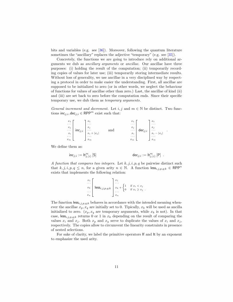
bits and variables (e.g. see [36]). Moreover, following the quantum literaturesometimes the “ancillary” replaces the adjective “temporary” (e.g. see [35]).

Concretely, the functions we are going to introduce rely on additional ar-guments we dub as ancillary arguments or ancillae. Our ancillae have threepurposes: (i) holding the result of the computation; (ii) temporarily record-ing copies of values for later use; (iii) temporarily storing intermediate results.Without loss of generality, we use ancillae in a very disciplined way by respect-ing a protocol in order to make easier the understanding. First, all ancillae aresupposed to be initialized to zero (or in other words, we neglect the behaviourof functions for values of ancillae other than zero.) Last, the ancillae of kind (ii)and (iii) are set back to zero before the computation ends. Since their specifictemporary use, we dub them as temporary arguments.

General increment and decrement. Let i, j and m ∈ N be distinct. Two func-tions incj;i, decj;i ∈ RPPm exist such that:

x1

· · ·xj· · ·xi· · ·xm

incj;i

x1

· · ·xj· · ·xi + |xj |· · ·xm

and

x1

· · ·xj· · ·xi· · ·xm

decj;i

x1

· · ·xj· · ·xi − |xj |· · ·xm

.

We define them as:

incj;i := Itmj,〈i〉 [S] decj;i := Itmj,〈i〉 [P] .

A function that compares two integers. Let k, j, i, p, q be pairwise distinct suchthat k, j, i, p, q ≤ n, for a given arity n ∈ N. A function lessi,j,p,q;k ∈ RPPn

exists that implements the following relation:

x1

· · ·xk

· · ·xn

lessi,j,p,q;k

x1

· · ·xk +

{1 if xi < xj0 if xi ≥ xj .

· · ·xn

The function lessi,j,p,q;k behaves in accordance with the intended meaning when-ever the ancillae xp, xq are initially set to 0. Tipically, xk will be used as ancillainitialized to zero. (xp, xq are temporary arguments, while xk is not). In thatcase, lessi,j,p,q;k returns 0 or 1 in xk depending on the result of comparing thevalues xi and xj . Both xp and xq serve to duplicate the values of xi and xj ,respectively. The copies allow to circumvent the linearity constraints in presenceof nested selections.

For sake of clarity, we label the primitive operators If and It by an exponentto emphasize the used arity.

11

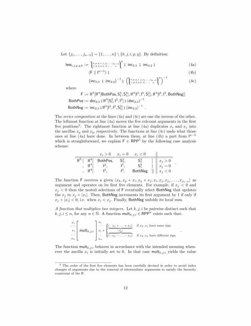
Let {j1, . . . , jn−5} = {1, . . . , n} \ {k, j, i, p, q}. By definition:

lessi,j,p,q;k :=k,p,q,i,j,j1,...,jn−5

1,2,3,4,5, 6 ,..., n

n # inc5;3 # inc4;2 # (4a)

(F ‖ In−5) # (4b)(inc5;3 # inc4;2

)−1 #(k,p,q,i,j,j1,...,jn−5

1,2,3,4,5, 6 ,..., n

n)−1

(4c)

where

F := If5[If4[BothPos,S31,S

31], If4[I3, I3,S3

1], If4[I3, I3,BothNeg]]

BothPos := dec2;3 # If3[S21, I

2, I2] # (dec2;3)−1

BothNeg := inc2;3 # If3[I2, I2,S25] # (inc2;3)

−1.

The series composition at the lines (4a) and (4c) are one the inverse of the other.The leftmost function at line (4a) moves the five relevant arguments in the firstfive positions3. The rightmost function at line (4a) duplicates xi and xj intothe ancillae xp and xq, respectively. The functions at line (4c) undo what thoseones at line (4a) have done. In between them, at line (4b) a part from In−5

which is straightforward, we explain F ∈ RPP5 by the following case analysisscheme:

xi > 0 xi = 0 xi < 0

If5 [ If4[ BothPos, S31, S3

1 ] xj > 0

, If4[ I3, I3, S31 ] xj = 0

, If4[ I3, I3, BothNeg ]] xj < 0

.

The function F receives a given 〈xk, xp + xi, xq + xj , xi, xj , xj1 , . . . , xjn−5〉 asargument and operates on its first five elements. For example, if xj < 0 andxj < 0 then the nested selections of F eventually select BothNeg that updatesthe xj to xj + |xi|. Then, BothNeg increments its first argument by 1 if only ifxj + |xi| < 0, i.e. when xi < xj . Finally, BothNeg unfolds its local sum.

A function that multiplies two integers. Let k, j, i be pairwise distinct such thatk, j, i ≤ n, for any n ∈ N. A function multk,j;i ∈ RPPn exists such that:

x1

· · ·xi

· · ·xn

multk,j;i

x1

· · ·

xi +

( xj + . . . + xj)︸ ︷︷ ︸

|xk|

if xk, xj have same sign

︷ ︸︸ ︷(−xj − . . .− xj) if xk, xj have different sign· · ·

xn

.

The function multk,j;i behaves in accordance with the intended meaning when-ever the ancilla xi is initially set to 0. In that case multk,j;i yields the value

3 The order of the first five elements has been carefully devised in order to avoid indexchanges of arguments due to the removal of intermediate arguments to satisfy the linearityconstraint of the If.

12

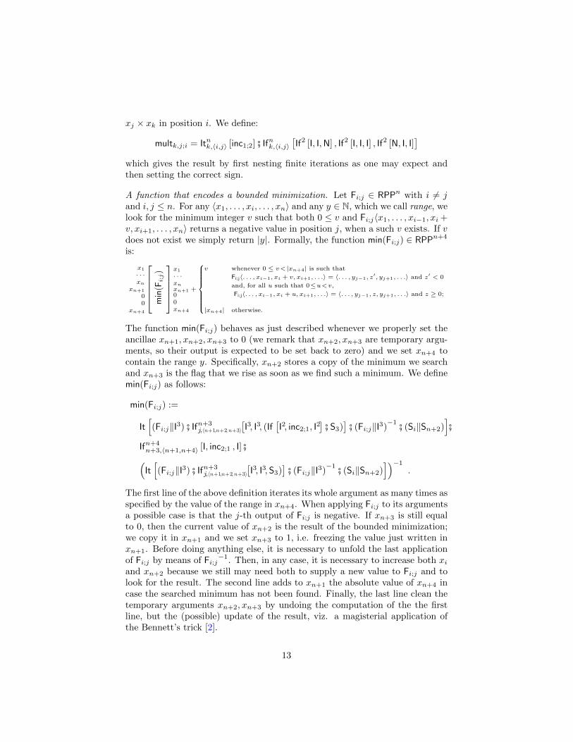
xj × xk in position i. We define:

multk,j;i = Itnk,〈i,j〉 [inc1;2] # Ifnk,〈i,j〉[If2 [I, I,N] , If2 [I, I, I] , If2 [N, I, I]

]which gives the result by first nesting finite iterations as one may expect andthen setting the correct sign.

A function that encodes a bounded minimization. Let Fi;j ∈ RPPn with i 6= jand i, j ≤ n. For any 〈x1, . . . , xi, . . . , xn〉 and any y ∈ N, which we call range, welook for the minimum integer v such that both 0 ≤ v and Fi;j〈x1, . . . , xi−1, xi +v, xi+1, . . . , xn〉 returns a negative value in position j, when a such v exists. If vdoes not exist we simply return |y|. Formally, the function min(Fi;j) ∈ RPPn+4

is:

x1

· · ·xn

xn+1

00

xn+4

min

(Fi;j)

x1

· · ·xnxn+1 +

v whenever 0 ≤ v< |xn+4| is such that

Fi;j〈. . . , xi−1, xi + v, xi+1, . . .〉 = 〈. . . , yj−1, z′, yj+1, . . .〉 and z′ < 0

and, for all u such that 0≤u<v,

Fi;j〈. . . , xi−1, xi + u, xi+1, . . .〉 = 〈. . . , yj−1, z, yj+1, . . .〉 and z ≥ 0;

|xn+4| otherwise.

00xn+4

The function min(Fi;j) behaves as just described whenever we properly set theancillae xn+1, xn+2, xn+3 to 0 (we remark that xn+2, xn+3 are temporary argu-ments, so their output is expected to be set back to zero) and we set xn+4 tocontain the range y. Specifically, xn+2 stores a copy of the minimum we searchand xn+3 is the flag that we rise as soon as we find such a minimum. We definemin(Fi;j) as follows:

min(Fi;j) :=

It[(Fi;j‖I3) # Ifn+3

j,〈n+1,n+2, n+3〉

[I3, I3, (If

[I2, inc2;1, I

2]# S3)

]# (Fi;j‖I3)

−1 # (Si‖Sn+2)]#

Ifn+4n+3,〈n+1,n+4〉 [I, inc2;1 , I] #(It[(Fi;j‖I3) # Ifn+3

j,〈n+1,n+2, n+3〉

[I3, I3,S3)

]# (Fi;j‖I3)

−1 # (Si‖Sn+2)])−1

.

The first line of the above definition iterates its whole argument as many times asspecified by the value of the range in xn+4. When applying Fi;j to its argumentsa possible case is that the j-th output of Fi;j is negative. If xn+3 is still equalto 0, then the current value of xn+2 is the result of the bounded minimization;we copy it in xn+1 and we set xn+3 to 1, i.e. freezing the value just written inxn+1. Before doing anything else, it is necessary to unfold the last applicationof Fi;j by means of Fi;j

−1. Then, in any case, it is necessary to increase both xiand xn+2 because we still may need both to supply a new value to Fi;j and tolook for the result. The second line adds to xn+1 the absolute value of xn+4 incase the searched minimum has not been found. Finally, the last line clean thetemporary arguments xn+2, xn+3 by undoing the computation of the the firstline, but the (possible) update of the result, viz. a magisterial application ofthe Bennett’s trick [2].

13

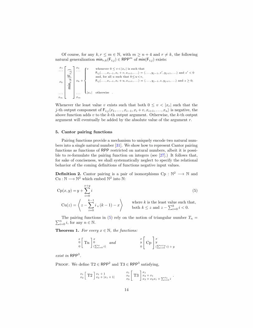
Of course, for any k, r ≤ m ∈ N, with m ≥ n + 4 and r 6= k, the followingnatural generalization minr;k(Fi;j) ∈ RPPm of min(Fi;j) exists:

x1

· · ·

xk

· · ·xm

min

r;k

(Fi;j)

x1

· · ·

xk +

v whenever 0 ≤ v< |xr| is such that

Fi;j〈. . . , xi−1, xi + v, xi+1, . . .〉 = 〈. . . , yj−1, z′, yj+1, . . .〉 and z′ < 0

and, for all u such that 0≤u<v,

Fi;j〈. . . , xi−1, xi + u, xi+1, . . .〉 = 〈. . . , yj−1, z, yj+1, . . .〉 and z ≥ 0;

|xr| otherwise .· · ·xm

Whenever the least value v exists such that both 0 ≤ v < |xr| such that thej-th output component of Fi;j〈x1, . . . , xi−1, xi + v, xi+1, . . . , xn〉 is negative, theabove function adds v to the k-th output argument. Otherwise, the k-th outputargument will eventually be added by the absolute value of the argument r.

5. Cantor pairing functions

Pairing functions provide a mechanism to uniquely encode two natural num-bers into a single natural number [31]. We show how to represent Cantor pairingfunctions as functions of RPP restricted on natural numbers, albeit it is possi-ble to re-formulate the pairing function on integers (see [27].) It follows that,for sake of conciseness, we shall systematically neglect to specify the relationalbehavior of the coming definitions of functions negative input values.

Definition 2. Cantor pairing is a pair of isomorphisms Cp : N2 −→ N andCu : N −→ N2 which embed N2 into N:

Cp(x, y) = y +

x+y∑i=0

i (5)

Cu(z) =

⟨z −

k−1∑i=0

i ,,, (k − 1)− x

⟩where k is the least value such that,

both k ≤ z and z −∑k

i=0 i < 0.

The pairing functions in (5) rely on the notion of triangular number Tn =∑ni=0 i, for any n ∈ N.

Theorem 1. For every x ∈ N, the functions:

x0

0

[Tn

]x0

(∑xi=0 i)

andxy

0

[Cp

]xy

(∑x+yi=0 i) + y

exist in RPP3.

Proof. We define T2 ∈ RPP2 and T3 ∈ RPP3 satisfying,

x1

x2

[T2]x1 + 1x2 + |x1 + 1|

x1

x2

x3

[T3

]x1

x2 + x1

x3 + x2x1 +∑x1i=0 i

.

14

by T2 := S21#inc

21;2 and T3 := It31,〈2,3〉 [T2]. Therefore, we can define the functions

as follows Tn := T3 #dec31;2 and Cp := inc3

2;1 #1, 2, 3

1, 3, 2

3

# Tn.

We now show that an operator kCu exists which we can think of as being thekernel of Cu. It allows to compute the least value k that generates the (least)

triangular number∑k

i=0 i which let z − (∑k

i=0 i) < 0.

Lemma 2 (The kernel kCu). A function kCu ∈ RPP9 exists such that:

x1

0

07

[kCu

]x1

0 + least v < x1 such that x1 − (∑vi=0 i) < 0

07

for every x1 ∈ N.

Proof. There exists H3;4 ∈ RPP4 such that:

00

x3

x4

[H3;4

]00x3

x4 −∑x3i=0 i

for every x3, x4 ∈ N. By Theorem 1, we define

H3;4 =

(1, 2, 3, 43, 2, 1, 4

4

# (Tn‖I))

# dec43;4 #

(1, 2, 3, 41, 2, 3, 4

4

# (Tn‖I))−1

.

The final step is using H3;4 as the parameter of the bounded minimization:

kCu =

(1, 2, 3, 4, 5, 6, 7, 8, 98, 2, 3, 4, 5, 6, 7, 1, 9

9

# (min(H3;4)‖I1)

)# inc9

5;9 #(1, 2, 3, 4, 5, 6, 7, 8, 98, 2, 3, 4, 5, 6, 7, 1, 9

9

# (min(H3;4)‖I1)

)−1

#1, 2, 3, 4, 5, 6, 7, 8, 9

1, 9, 3, 4, 5, 6, 7, 8, 2

9

.

Theorem 3 (Representing Cu : N2 −→ N in RPP). A function Cu ∈ RPP11

exists such that, for every z ∈ N:

z

0

0

08

Cu

z

z − (∑v−1i=0 i)

(v − 1)− (z − (∑v−1i=0 i))

08 ,

where v is the least value such that v ≤ z and z− (∑v

i=0 i) < 0. So z− (∑v−1

i=0 i)is the first component of the pair that z represents under Cantor’s pairing and(v − 1)− (z − (

∑v−1i=0 i)) is the second one.

Proof. It is enough to follow the standard pattern: (i) start by rearranging

inputs; (ii) find v using kCu ∈ RPP9; (iii) compute∑v−1

i=0 i by Tn ∈ RPP3; (iv)

compute (v − 1) − (z − (∑v−1

i=0 i)) and z − (∑v−1

i=0 i); (v) a permutation whichrearranges the outputs as required concludes the definition.

We remark that Theorem 1, Lemma 2 and Theorem 3 can be extended to afunctions that operate on values of Z, not only of N, suitably managing signs.We refer to [27] for some discussions on the point.

15

6. Expressiveness of RPP

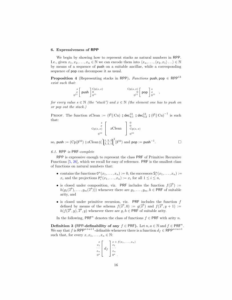
We begin by showing how to represent stacks as natural numbers in RPP.I.e., given x1, x2, . . . , xn ∈ N we can encode them into 〈xn, . . . , 〈x2, x1〉 . . .〉 ∈ Nby means of a sequence of push on a suitable ancillae, while a correspondingsequence of pop can decompose it as usual.

Proposition 4 (Representing stacks in RPP). Functions push, pop ∈ RPP13

exist such that:

sx

011

[push

]Cp(s, x)0011

Cp(s, x)0

011

[pop

]sx011

,

for every value s ∈ N (the “stack”) and x ∈ N (the element one has to push onor pop out the stack.)

Proof. The function zClean := (I2‖Cu) # dec134;1 # dec13

5;2 # (I2‖Cu)−1

is suchthat:

sx

Cp(s, x)

010

zClean

00Cp(s, x)

010

so, push := (Cp‖I10) # zClean #(1, 2, 3

3, 2, 1

3

‖I10) and pop := push−1.

6.1. RPP is PRF-complete

RPP is expressive enough to represent the class PRF of Primitive RecursiveFunctions [5, 26], which we recall for easy of reference. PRF is the smallest classof functions on natural numbers that:

• contains the functions 0n(x1, . . . , xn) := 0, the successors Sni (x1, . . . , xn) :=xi and the projections Pni (x1, . . . , xn) := xi for all 1 ≤ i ≤ n,

• is closed under composition, viz. PRF includes the function f(−→x ) :=h(g1(−→x ), . . . , gm(−→x ))) whenever there are g1, . . . , gm, h ∈ PRF of suitablearity, and

• is closed under primitive recursion, viz. PRF includes the function fdefined by means of the schema f(−→x , 0) := g(−→x ) and f(−→x , y + 1) :=h(f(−→x , y),−→x , y) whenever there are g, h ∈ PRF of suitable arity.

In the following, PRFn denotes the class of functions f ∈ PRF with arity n.

Definition 3 (RPP-definability of any f ∈ PRF). Let n, a ∈ N and f ∈ PRFn.We say that f is RPPn+a+1-definable whenever there is a function df ∈ RPPn+a+1

such that, for every x, x1, . . . , xn ∈ N:

xx1

· · ·xn

0a

df

x + f(x1, . . . , xn)x1

· · ·xn

0a .

16

xx1

· · ·xn

0m

k

r1· · ·

ri−1

0

ri+1

· · ·rk

g∗i

xx1

· · ·xn

0m

r1· · ·ri−1

gi(x1, . . . , xn)ri+1

· · ·rk

xx1

· · ·xn

0m

k

0

· · ·0

h∗

x + ◦[h, g1, . . . , gk](x1, . . . , xn)x1

· · ·xn

0m

g1(x1, . . . , xn)

· · ·gk(x1, . . . , xn)

xx1

· · ·xn

0m

k

0

· · ·0

G

xx1

· · ·xn

0m

g1(x1, . . . , xn)

· · ·gk(x1, . . . , xn)

xx1

· · ·xn

0m

0k

H

x + ◦[h, g1, . . . , gk](x1, . . . , xn)x1

· · ·xn

0m

0k

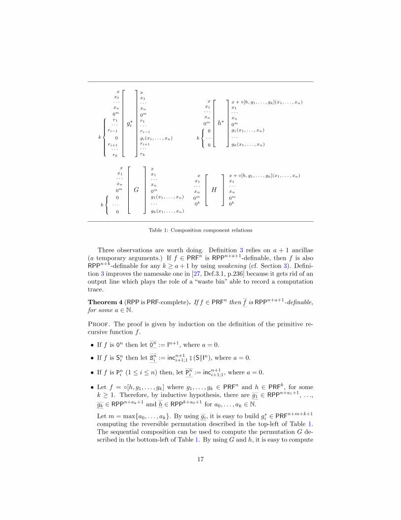
Table 1: Composition component relations

Three observations are worth doing. Definition 3 relies on a + 1 ancillae(a temporary arguments.) If f ∈ PRFn is RPPn+a+1-definable, then f is alsoRPPn+k-definable for any k ≥ a+ 1 by using weakening (cf. Section 3). Defini-tion 3 improves the namesake one in [27, Def.3.1, p.236] because it gets rid of anoutput line which plays the role of a “waste bin” able to record a computationtrace.

Theorem 4 (RPP is PRF-complete). If f ∈ PRFn then f is RPPn+a+1-definable,for some a ∈ N.

Proof. The proof is given by induction on the definition of the primitive re-cursive function f .

• If f is 0n then let 0n := In+1, where a = 0.

• If f is Sni then let Sni := incn+1i+1;1 # (S‖In), where a = 0.

• If f is Pni (1 ≤ i ≤ n) then, let Pni := incn+1i+1;1, where a = 0.

• Let f = ◦[h, g1, . . . , gk] where g1, . . . , gk ∈ PRFn and h ∈ PRFk, for somek ≥ 1. Therefore, by inductive hypothesis, there are g1 ∈ RPPn+a1+1, . . .,

gk ∈ RPPn+ak+1 and h ∈ RPPk+a0+1 for a0, . . . , ak ∈ N.

Let m = max{a0, . . . , ak}. By using gi, it is easy to build g∗i ∈ PRFn+m+k+1

computing the reversible permutation described in the top-left of Table 1.The sequential composition can be used to compute the permutation G de-scribed in the bottom-left of Table 1. By using G and h, it is easy to compute

17

xx1

· · ·xn

0· · ·

0

04

f

f(x1, . . . , xn)

x1

· · ·xn

0· · ·0

max{ag, ah, 13}

04

0r

x1

· · ·xn−1

i

0a−4

S

hstep

0

h(r, x1, . . . , xn−1, i)x1

· · ·xn−1

i + 1

0a−4

〈r,S〉

Table 2: Primitive Recursion Components

h∗ in the top-right of Table 1. Last, H ∈ RPPn+(m+k)+1 in the bottom-rightof Table 1 is ◦[h, g1, . . . , gk] and we define it as h∗ #G−1.

H improves the representation of composition sketched in [27] because itreduces the number of ancillae by re-using them to compute one after theother g1, . . . , gk ∈ PRFn and h ∈ PRFk.

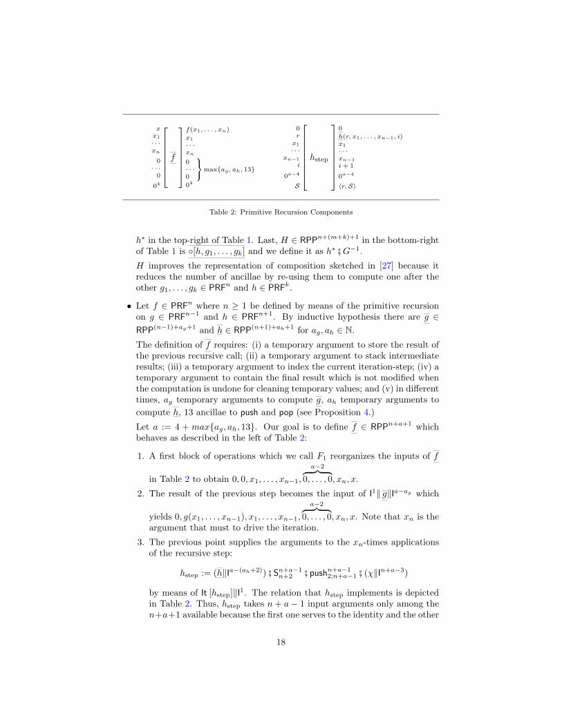
• Let f ∈ PRFn where n ≥ 1 be defined by means of the primitive recursionon g ∈ PRFn−1 and h ∈ PRFn+1. By inductive hypothesis there are g ∈RPP(n−1)+ag+1 and h ∈ RPP(n+1)+ah+1 for ag, ah ∈ N.

The definition of f requires: (i) a temporary argument to store the result ofthe previous recursive call; (ii) a temporary argument to stack intermediateresults; (iii) a temporary argument to index the current iteration-step; (iv) atemporary argument to contain the final result which is not modified whenthe computation is undone for cleaning temporary values; and (v) in differenttimes, ag temporary arguments to compute g, ah temporary arguments to

compute h, 13 ancillae to push and pop (see Proposition 4.)

Let a := 4 + max{ag, ah, 13}. Our goal is to define f ∈ RPPn+a+1 whichbehaves as described in the left of Table 2:

1. A first block of operations which we call F1 reorganizes the inputs of f

in Table 2 to obtain 0, 0, x1, . . . , xn−1,

a−2︷ ︸︸ ︷0, . . . , 0, xn, x.

2. The result of the previous step becomes the input of I1‖ g‖Ia−ag which

yields 0, g(x1, . . . , xn−1), x1, . . . , xn−1,

a−2︷ ︸︸ ︷0, . . . , 0, xn, x. Note that xn is the

argument that must to drive the iteration.

3. The previous point supplies the arguments to the xn-times applicationsof the recursive step:

hstep := (h‖Ia−(ah+2)) # Sn+a−1n+2 # pushn+a−1

2;n+a−1 # (χ‖In+a−3)

by means of It [hstep]‖I1. The relation that hstep implements is depictedin Table 2. Thus, hstep takes n+ a− 1 input arguments only among then+a+1 available because the first one serves to the identity and the other

18

one drives the iteration. The function of hstep first applies h and then re-organizes arguments for the next iteration. Specifically, (i) it incrementsthe step-index in the argument of position (n+2), (ii) it pushes the resultof the previous step, which is in position 2, on top of the stack , whichis in its last ancilla, (iii) it exchanges the first two arguments, the firstone containing the result of the last iterative step and the second onecontaining a fresh zero produced by push.

4. We get 0, f(x1, . . . , xn), x1, . . . , xn−1, xn,

a−2︷ ︸︸ ︷0, . . . , 0, xn, x from the previous

point. We add the result to the last line by means of inc2;n+a+1 by yielding

0, f(x1, . . . , xn), x1, . . . , xn−1, xn,

a−2︷ ︸︸ ︷0, . . . , 0, xn, x+ f(x1, . . . , xn).

5. We then conclude by unwinding the first three steps.

Summing up, h is:

F1#(I1‖ g‖Ia−ag

)#(It [hstep]‖I1

)#inc2;n+a+1#

(It [hstep]‖I1

)−1#(I1‖ g‖Ia−ag

)−1#F1−1 .

6.2. RPP is PRF-sound

The mere intuition should support the evidence that every f ∈ RPP has arepresentative inside PRF we can obtain via the bijection which exists betweenZ and N. More precisely, every RPP-permutation can be represented as a PRF-endofunction on tuples of natural numbers which encode integers. Details onhow formalizing the embedding of RPP into PRF are in [27].

7. Conclusions

7.1. The intensioanl nature of the functions in RPP

Let A be the Ackermann function, example of total computable functionwith two arguments that cannot belong to PRF because its growth rate is toohigh. Kuznekov shows that a primitive recursive function F exists with inputarity 1 such that F−1(x) = A(x, x). It is worth to remark that the inverse ofF is not primitive recursive, because A is not. References are not immediate,because the original result [15] is in Russian: some details about Kuznekov’sproof are in [27, 33]. Moreover in [34, Exercise 5.7, p.25] Kuznecov’s result isslightly reformulated by the statement saying that“primitive recursive functionsdo not form a group under composition.”

By Theorem 4, the function:

wz

0k

[F

]w + F (z)z

0k

19

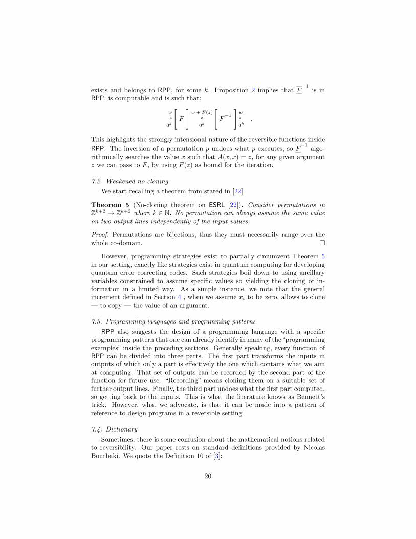
exists and belongs to RPP, for some k. Proposition 2 implies that F−1

is inRPP, is computable and is such that:

wz

0k

[F

]w + F (z)

z

0k

[F−1

]wz

0k.

This highlights the strongly intensional nature of the reversible functions inside

RPP. The inversion of a permutation p undoes what p executes, so F−1

algo-rithmically searches the value x such that A(x, x) = z, for any given argumentz we can pass to F , by using F (z) as bound for the iteration.

7.2. Weakened no-cloning

We start recalling a theorem from stated in [22].

Theorem 5 (No-cloning theorem on ESRL [22]). Consider permutations inZk+2 → Zk+2 where k ∈ N. No permutation can always assume the same valueon two output lines independently of the input values.

Proof. Permutations are bijections, thus they must necessarily range over thewhole co-domain.

However, programming strategies exist to partially circumvent Theorem 5in our setting, exactly like strategies exist in quantum computing for developingquantum error correcting codes. Such strategies boil down to using ancillaryvariables constrained to assume specific values so yielding the cloning of in-formation in a limited way. As a simple instance, we note that the generalincrement defined in Section 4 , when we assume xi to be zero, allows to clone— to copy — the value of an argument.

7.3. Programming languages and programming patterns

RPP also suggests the design of a programming language with a specificprogramming pattern that one can already identify in many of the“programmingexamples” inside the preceding sections. Generally speaking, every function ofRPP can be divided into three parts. The first part transforms the inputs inoutputs of which only a part is effectively the one which contains what we aimat computing. That set of outputs can be recorded by the second part of thefunction for future use. “Recording” means cloning them on a suitable set offurther output lines. Finally, the third part undoes what the first part computed,so getting back to the inputs. This is what the literature knows as Bennett’strick. However, what we advocate, is that it can be made into a pattern ofreference to design programs in a reversible setting.

7.4. Dictionary

Sometimes, there is some confusion about the mathematical notions relatedto reversibility. Our paper rests on standard definitions provided by NicolasBourbaki. We quote the Definition 10 of [3]:

20

Let f be a mapping of A into B. The mapping f is said to beinjective, or an injection, if any two distinct elements of A havedistinct images under f . The mapping f is said to be surjective, ora surjection if f(A) = B. If f is both injective and surjective, it issaid to be bijective, or a bijection.

and some phrases, that can be found few lines below:

If f is bijective, we sometimes say that f puts A and B in one-to-onecorrespondence. A bijection of A onto A is called a permutation ofA.

We are convinced that the definitions above are standard, but we remarkthat injection is sometimes used to mean inclusion (see [8, p.31]) and one-to-oneis used to mean Bourbaki’s injective function.

The notion of invertible function is much less standard and is used in manyways in literature. Such an adjective is associated either to injective mapswhenever the domain-codomain of the inverse does not matter (cf. [5, p.2]), orto bijective maps (whenever domain-codomain matter, e.g. in [18] invertible isintended as the conjunction of left and right invertible). It is worth notice that,in both cases, the inversion of a computable function is computable.

Yet, we remark that many algebraic and categorical notions are related tothe above ones (see [17]) and, finally, that reversible function means functionthat can be defined via aReversible Turing Machine.

7.5. Future work

Firstly, a comparison between the expressiveness of ESRL and RPP is un-derway. Secondly, we would like to extend RPP in many ways without leavingtotal computations. One extension would consist on adding primitives able tohide ancillary variables by fixing their value, so to simplify programming in thelines of [35]. Another would allow the definition of functions with different ar-ity and co-arity, by including some specific bijections as primitives. This waywe would extend RPP to a class with functions that would not necessarily bepermutations. Thirdly, of course, we are working on a natural extension of RPPwhich is complete with respect to Kleene partial recursive functions.

References

[1] H. B. Axelsen and R. Gluck. What do reversible programs compute?In 14th International Conference on Foundations of Software Science andComputational Structures, volume 6604 of Lecture Notes in Computer Sci-ence, pages 42–56. Springer, 2011.

[2] C. H. Bennett. Logical reversibility of computation. IBM J. Res. Develop.,17:525–532, 1973.

[3] N. Bourbaki. Elements of mathematics. Theory of sets. Addison-Wesley,1968. Translated from the French.

21

[4] F. B. Cannonito and M. Finkelstein. On primitive recursive permutationsand their inverses. Journal of Symbolic Logic, 34(4):634–638, 12 1969.

[5] N. Cutland. Computability: An Introduction to Recursive Function Theory.Cambridge University Press, 1980.

[6] P. Giannini, E. Merelli, and A. Troina. Interactions between computerscience and biology. Theoretical Computer Science, 587:1 – 2, 2015. Inter-actions between Computer Science and Biology.

[7] S. Guerrini, S. Martini, and A. Masini. Towards A theory of quantumcomputability. CoRR, abs/1504.02817, 2015.

[8] P. Halmos. Naive Set Theory. Undergraduate Texts in Mathematics.Springer, 1960.

[9] G. Jacopini and P. Mentrasti. Generation of invertible functions. Theor.Comput. Sci., 66(3):289–297, 1989.

[10] G. Jacopini and G. Sontacchi. General recursive functions in a very simplyinterpretable typed lambda-calculus. Theor. Comput. Sci., 121(1&2):169–178, 1993.

[11] R. P. James and A. Sabry. Information effects. In Proceedings of the39th ACM SIGPLAN-SIGACT Symposium on Principles of ProgrammingLanguages, POPL 2012, Philadelphia, Pennsylvania, USA, January 22-28,2012, pages 73–84, 2012.

[12] I. Kalimullin. Computability and Models: Perspectives East and West,chapter On Primitive Recursive Permutations, pages 249–258. Springer,2003.

[13] V. V. Koz’minykh. On the representation of partial recursive functions assuperpositions. Algebra and Logic, 11(3):153–167, 1972.

[14] V. V. Koz’minykh. Representation of partial recursive functions with cer-tain conditions in the form of superpositions. Algebra and Logic, 13(4):238–240, 1974.

[15] A. V. Kuznecov. On primitive recursive functions of large oscillation. Dok-lady Akademii Nauk SSSR, 71:233–236, 1950. In russian.

[16] Y. Lafont. Towards an algebraic theory of boolean circuits. Journal of Pureand Applied Algebra, 184(2–3):257–310, 2003.

[17] S. Lane. Categories for the Working Mathematician. Graduate Texts inMathematics. Springer New York, 1998.

[18] S. Lane and G. Birkhoff. Algebra. Chelsea Publishing Series. Chelsea Pub-lishing Company, 1999.

22

[19] Y. Lecerf. Machines de turing reversibles. Comptes Rendus Hebdomadairesdes Seances de L’academie des Sciences, 257:2597–2600, 1963.

[20] A. I. Malcev. Algorithms and recursive functions. Wolters-Noordhoff, 1970.Translated from the first Russian ed. by Leo F. Boron, with the collabora-tion of Luis E. Sanchis, John Stillwell and Kiyoshi Iseki.

[21] A. B. Matos. Linear programs in a simple reversible language. Theor.Comput. Sci., 290(3):2063–2074, 2003.

[22] A. B. Matos. Register reversible languages.Available at http://www.dcc.fc.up.pt/~acm/questionsv.pdf, January2016.

[23] J. McCarthy. The inversion of functions defined by turing machines. InC. Shannon and J. McCarthy, editors, Automata Studies, Annals of Math-ematical Studies, 34, pages 177–181. Princeton University Press, 1956.

[24] A. R. Meyer and D. M. Ritchie. The complexity of loop programs. InProceedings of the 1967 22Nd National Conference, ACM ’67, pages 465–469, New York, NY, USA, 1967. ACM.

[25] K. Morita. Reversible computing and cellular automata – a survey. Theo-retical Computer Science, 395(1):101 – 131, 2008.

[26] P. Odifreddi. Classical recursion theory: the theory of functions and setsof natural numbers. Studies in logic and the foundations of mathematics.North-Holland, 1989.

[27] L. Paolini, M. Piccolo, and L. Roversi. A class of reversible primitiverecursive functions. Electronic Notes in Theoretical Computer Science,322(18605):227–242, 2016.

[28] K. S. Perumalla. Introduction to Reversible Computing. Chapman &Hall/CRC Computational Science. Taylor & Francis, 2013.

[29] J. Robinson. General recursive functions. Proceedings of the AmericanMathematical Society, 1:703–718, 1950.

[30] H. Rogers. Theory of recursive functions and effective computability.McGraw-Hill series in higher mathematics. McGraw-Hill, 1967.

[31] A. L. Rosenberg. The Pillars of Computation Theory: State, Encoding,Nondeterminism. Springer Publishing Company, Incorporated, 1st edition,2009.

[32] P. Rozsa. Recursive functions. Academic Press, 1967.

[33] S. G. Simpson. Foundations of mathematics. De-partement of Mathematics, University of Pennsylvania.http://www.personal.psu.edu/t20/notes/fom.pdf, 2009.

23

[34] R. Soare. Recursively Enumerable Sets and Degrees: A Study of ComputableFunctions and Computably Generated Sets. Perspectives in MathematicalLogic. Springer, 1987.

[35] M. K. Thomsen, R. Kaarsgaard, and M. Soeken. Ricercar: A language

for describing andA rewriting reversible circuits with ancillae and its per-mutation semantics. In J. Krivine and J.-B. Stefani, editors, ReversibleComputation: 7th International Conference, RC 2015, Grenoble, France,July 16-17, 2015, Proceedings, number 9138 in Lecture Notes in TheoreticalComputer Science, pages 200–215, 2015.

[36] T. Toffoli. Reversible computing. In J. W. de Bakker and J. van Leeuwen,editors, Automata, Languages and Programming, 7th Colloquium, Noord-weijkerhout, The Netherland, July 14-18, 1980, Proceedings, volume 85 ofLecture Notes in Computer Science, pages 632–644. Springer, 1980.

[37] T. Yokoyama, H. B. Axelsen, and R. Gluck. Principles of a reversible pro-gramming language. In A. Ramırez, G. Bilardi, and M. Gschwind, editors,Proceedings of the 5th Conference on Computing Frontiers, 2008, Ischia,Italy, May 5-7, 2008, pages 43–54. ACM, 2008.

[38] M. Zorzi. On quantum lambda calculi: a foundational per-spective. Mathematical Structures in Computer Science, 2014.http://dx.doi.org/10.1017/S0960129514000425.

24