A Class of Population Covariance Matrices for Monte Carlo Simulation

Ke-Hai Yuan∗, Kentaro Hayashi∗∗ and Hirokazu Yanagihara∗∗∗

∗Department of Psychology

University of Notre Dame

Notre Dame, Indiana 46556, USA

∗∗∗Department of Psychology

University of Hawaii

Honolulu, Hawaii 96822-2294, USA

∗∗∗Department of Social Systems and Management

Graduate School of Systems and Information Engineering

University of Tsukuba

1-1-1 Tennodai, Tsukuba, Ibaraki 305-8573, Japan

March 31, 2006

The research was supported by NSF grant DMS-0437167, the James McKeen Cattell Fund

and the Japan Ministry of Education, Science, Sports and Culture Grant-in-Aid for Young

Scientists (B) #17700274. Correspondence concerning this article should be addressed to

Ke-Hai Yuan (kyuan@nd.edu).

Abstract

Model evaluation in covariance structure analysis is critical before the results can be

trusted. Due to finite sample sizes and unknown distributions of practical data, existing

conclusion regarding a particular statistic may not be applicable in practice. The bootstrap

procedure automatically takes care of the unknown distribution and, for a given sample size,

also provides more accurate results than those based on standard asymptotics. But it needs

a matrix to play the role of the population covariance matrix. The closer the matrix is

to the true population covariance matrix, the more valid the bootstrap inference is. The

current paper proposes a class of covariance matrices by combining theory and data. Thus,

a proper matrix from this class is closer to the true population covariance matrix than those

constructed by any existing methods. Each of the covariance matrices is easy to generate

and also satisfies several desired properties. Examples verify the properties of the matrices

and illustrate the details for creating a matrix with a given amount of misspecification.

Keywords: Bootstrap, model misspecification, noncentrality parameter.

1. Introduction

Structural equation modeling (SEM), covariance structure analysis (CSA) in particular,

has been widely used in the social and behavioral sciences (Bentler & Dudgeon, 1996; Bollen,

2002; MacCallum & Austin, 2000). The advantage of CSA is that manifest variables, latent

variables as well as measurement errors can be modeled and tested simultaneously. In ap-

plying CSA models, model evaluation is critical before the results can be trusted. Various

procedures have been developed for such purposes (Bentler, 1983; Bentler & Dijkstra, 1985;

Browne, 1984; Kano, Berkane, & Bentler, 1990; Joreskog, 1969; Satorra, 1989; Satorra &

Bentler, 1994; Shapiro & Browne, 1987; Yuan & Bentler, 1997, 1998, 1999a). The behaviors

of several commonly used statistics for overall model evaluation are extensively studied by

either asymptotics (Amemiya & Anderson, 1990; Browne & Shapiro, 1988; Shapiro, 1983;

Yuan & Bentler, 1999b) or simulation (see Bentler & Yuan, 1999; Chou, Bentler & Satorra,

1991; Curran, West & Finch, 1996; Hu, Bentler, & Kano, 1992; Muthen & Kaplan, 1985;

Yuan & Bentler, 1998). However, the conclusion obtained may not be valid when applying

the statistics to a practical data. For example, the asymptotic robustness condition for the

likelihood ratio statistic (Amemiya & Anderson, 1990; Browne & Shapiro, 1988) may not be

satisfied in any real data analysis. Similarly, the data generation scheme in most simulation

studies may rend the rescaled statistic (Satorra & Bentler, 1994) to asymptotically follow

a chi-square distribution (Yuan & Bentler, 1999b), such obtained results may not apply to

real data (see Yuan & Hayashi, 2003). Of course, the validity of any asymptotic properties

is closely related to the sample size of the data, which is typically out of control in practice.

Even when the sample is normally distributed, the behavior of a statistic is also closely

related to the model and the population covariance matrix as well as their distance, as mea-

sured by a discrepancy function. When the model gradually departs from the population

covariance matrix, the likelihood ratio statistic is better described by a noncentral chi-square

distribution at beginning and then better described by a normal distribution (Yuan, Hayashi

& Bentler, 2005).

When the distribution of the sample is unknown or when the sample size is not large

enough, the bootstrap approach represents a promising alternative (Efron, 1979). The boot-

1

strap has demonstrated its potential in dealing with various problems that challenge tradi-

tional statistical methods (Efron & Tibshirani, 1993; Davison & Hinkley, 1997). Bootstrap

methods have been applied to covariance structure models by various authors. Beran and

Srivastava (1985) set out the theoretical foundation for bootstrap inference about covariance

matrices in general. Bollen and Stine (1993) introduced the bootstrap approach to studying

the distribution of test statistics and fit indices and clearly demonstrated the importance of

choosing the proper matrix in playing the role of bootstrap population. Chatterjee (1984),

Boomsma (1986) and Bollen and Stine (1990) used bootstrap to study standard errors in co-

variance structure models. Yung and Bentler (1996) reviewed many applications of bootstrap

in covariance structure analysis. Yung and Bentler (1996), Yuan and Hayashi (2003) and

Yuan and Marshall (2004) used bootstrap to estimate power and lack of fit in CSA. Enders

(2002) used bootstrap to study the goodness of fit in CSA with missing data. In contrast

with inferences that are based on normal theory maximum likelihood (ML), the bootstrap

approach does not assume normally distributed data. Even when data are normally dis-

tributed, at a given sample size, the bootstrap may give more accurate results than those

based on standard asymptotics due to its second order accuracy (see Hall & Titterington,

1989).

Let x1, x2, · · ·, xn be a sample with a sample covariance matrix S whose population

counterpart is Σ0. Conditional on the sample, the bootstrap repeatedly draw samples from

a known empirical distribution function. This empirical distribution plays the role of the

“population” for the bootstrap samples. Because Σ0 is generally unknown, one has to find

an alternative Sa to play the role of Σ0. With a given Sa, the remainder of the bootstrap is

standard. For example, xi can be transformed to x(a)i by

x(a)i = S1/2

a S−1/2xi, i = 1, 2, · · · , n, (1)

where S1/2a is a p×p matrix satisfying (S1/2

a )(S1/2a )′ = Sa. The following steps are to obtain the

bootstrap samples by sampling with replacement from (x(a)1 ,x

(a)2 , . . . ,x(a)

n ) and to calculate

the sample covariance matrices S∗ of the bootstrap samples. Interesting statistics will be

generated when fitting the substantive model to S∗. Of course, the form of Sa is decided

by the purpose of the study. When studying the behavior of model statistics under the

2

null hypothesis Σ0 = Σ(θ0), one needs to choose Sa = Σ(θ) for an admissible θ (Beran &

Srivastava, 1985; Bollen & Stine, 1993). When studying the power of a statistic one needs

to choose a Sa to represent the interesting alternative hypothesis (Beran, 1986; Yuan &

Hayashi, 2003; Yuan & Marshall, 2004).

Different Sa’s correspond to different populations. Because any interesting model in

practice is inevitably misspecified, there is a lot of interest in the property of test statistics

with misspecified models. In particular, the population covariance matrix Σ0 = E(S) is

generally unknown while the behavior of a test statistic at Σ0 is of fundamental interest.

It would be nice if a Sa that is close to Σ0 can be obtained. With unavoidable model

misspecification, formal or informal cutoff values have been established to judge a model

based on fit indices. However, the distribution of almost all the fit indices are generally

unknown (Yuan, 2005), and bootstrap can be used to study their distributions or confidence

intervals. In such a study, alternative covariance matrices are needed. For example, if one

needs to understand the behavior of the sample RMSEA (Steiger & Lind, 1980) when its

population value is 0.05 or 0.08, alternative covariance matrices are needed to achieve the

desired population values.

Parallel to obtaining a Sa that plays the role of Σ0 in the bootstrap simulation, obtaining

a covariance matrix that is at a given distance from a model structure is of interest in Monte

Carlo studies, where there is generally no particular Σ0 to consider. In that direction, Satorra

and Saris (1985) obtained a Σ through setting a fixed parameter in Σ(θ) at an incorrect

value. Cudeck and Browne (1992) provided a procedure for obtaining a Σ that is at a given

distance from a model structure. Curran, West and Finch (1996) generated a Σ that contains

loadings in the population but not in the model. Yuan and Bentler (1997) generated a Σ by

a structure with three factors while the null hypothesis is a two-factor model. Fouladi (2000)

created a Σ by properly perturbing the structured covariance matrix. These approaches of

generating Σ’s might also be used in constructing a population covariance matrix in the

bootstrap simulation, but the resulting Σ’s are generally not as desired as the one to be

described in this paper.

We will provide a class of Sa’s by combining empirical information represented by S and

substantive theory represented by Σ(θ). In section 2 of this paper we give the form of the

3

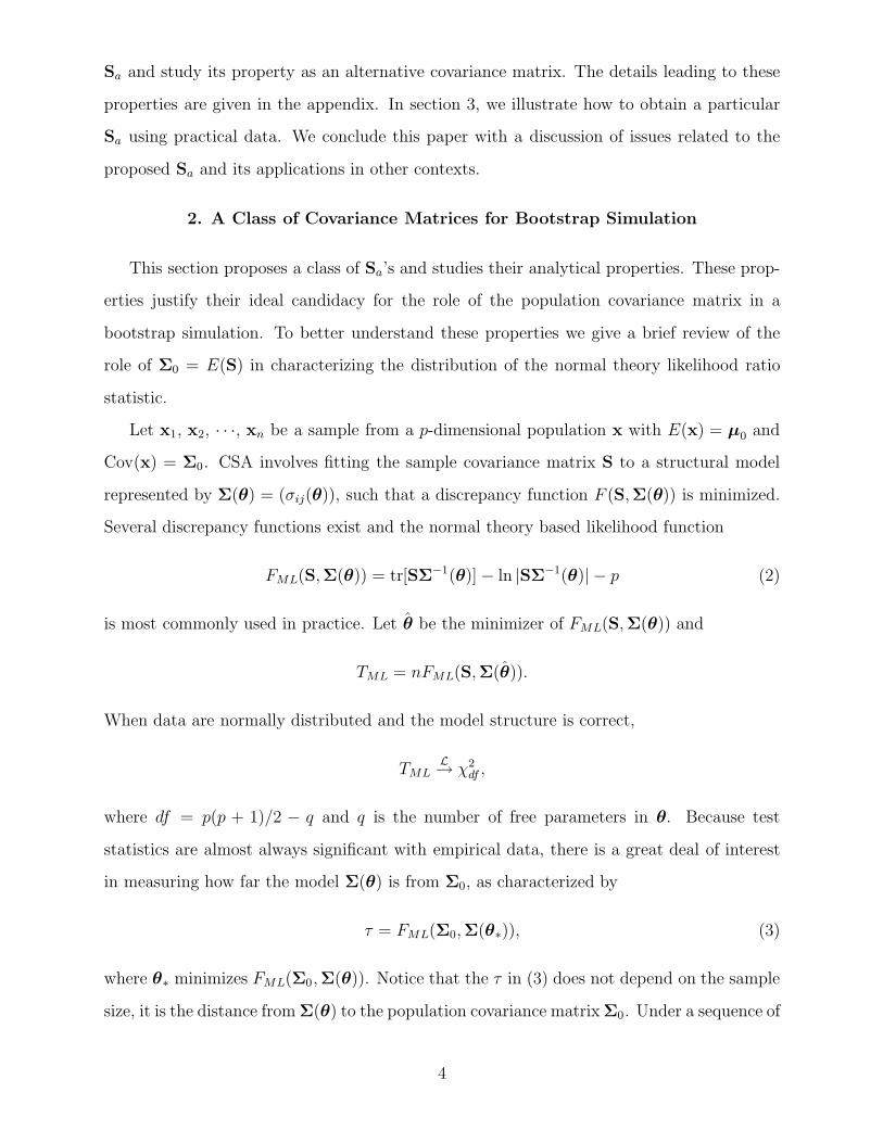
Sa and study its property as an alternative covariance matrix. The details leading to these

properties are given in the appendix. In section 3, we illustrate how to obtain a particular

Sa using practical data. We conclude this paper with a discussion of issues related to the

proposed Sa and its applications in other contexts.

2. A Class of Covariance Matrices for Bootstrap Simulation

This section proposes a class of Sa’s and studies their analytical properties. These prop-

erties justify their ideal candidacy for the role of the population covariance matrix in a

bootstrap simulation. To better understand these properties we give a brief review of the

role of Σ0 = E(S) in characterizing the distribution of the normal theory likelihood ratio

statistic.

Let x1, x2, · · ·, xn be a sample from a p-dimensional population x with E(x) = μ0 and

Cov(x) = Σ0. CSA involves fitting the sample covariance matrix S to a structural model

represented by Σ(θ) = (σij(θ)), such that a discrepancy function F (S,Σ(θ)) is minimized.

Several discrepancy functions exist and the normal theory based likelihood function

FML(S,Σ(θ)) = tr[SΣ−1(θ)] − ln |SΣ−1(θ)| − p (2)

is most commonly used in practice. Let θ be the minimizer of FML(S,Σ(θ)) and

TML = nFML(S,Σ(θ)).

When data are normally distributed and the model structure is correct,

TMLL→ χ2

df ,

where df = p(p + 1)/2 − q and q is the number of free parameters in θ. Because test

statistics are almost always significant with empirical data, there is a great deal of interest

in measuring how far the model Σ(θ) is from Σ0, as characterized by

τ = FML(Σ0,Σ(θ∗)), (3)

where θ∗ minimizes FML(Σ0,Σ(θ)). Notice that the τ in (3) does not depend on the sample

size, it is the distance from Σ(θ) to the population covariance matrix Σ0. Under a sequence of

4

local alternatives and normally distributed data (see Satorra & Saris, 1985; Steiger, Shapiro,

& Browne, 1985),

TMLL→ χ2

df(δ),

where δ = nτ . Thus

E(TML) ≈ nτ + df, (4)

where the approximation sign is due to a finite sample size. When data are not normally

distributed or when Σ0 is fixed, the result in (4) can be improved (Shapiro, 1983; Yuan et

al., 2005). For a p × p matrix A, let vech(A) be the vector that stacks the nonduplicated

elements of A by leaving out those above the diagonal, and denote σ(θ) = vech[Σ(θ)]. Let

Dp be the duplication matrix as defined by Magnus and Neudecker (1999, p. 49),

W0 =1

2D′

p(Σ−10 ⊗ Σ−1

0 )Dp, W(θ) =1

2D′

p[Σ−1(θ) ⊗ Σ−1(θ)]Dp,

Σ∗ = Σ(θ∗), W∗ = W(θ∗), σ∗ = ∂σ(θ∗)/∂θ′∗, Δij∗ = ∂2σij(θ∗)/∂θ∗∂θ′

∗,

G = Σ−1∗ Σ0Σ

−1∗ − 1

2Σ−1

∗ , H = (hij) = Σ∗ −Σ−1∗ Σ0Σ

−1∗ ,

M =1

2

p∑i=1

p∑j=1

hijΔij∗ and Π = Cov{vech[(x −μ0)(x − μ0)′]}.

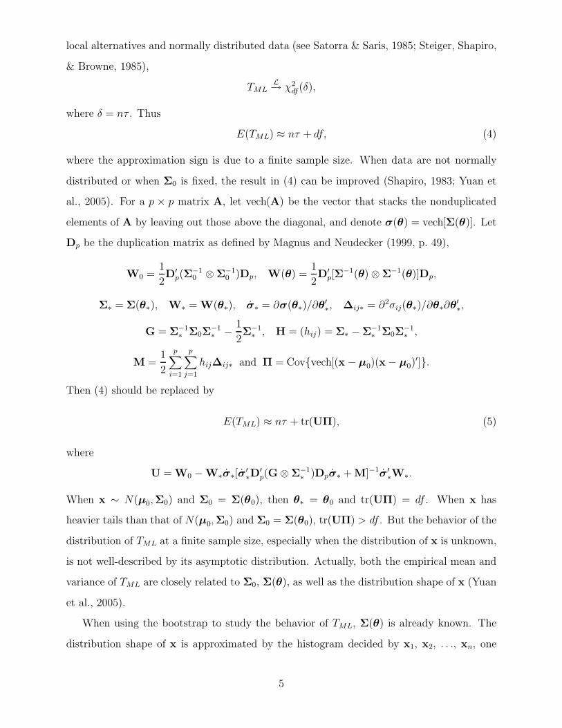
Then (4) should be replaced by

E(TML) ≈ nτ + tr(UΠ), (5)

where

U = W0 − W∗σ∗[σ′∗D

′p(G ⊗ Σ−1

∗ )Dpσ∗ + M]−1σ′∗W∗.

When x ∼ N(μ0,Σ0) and Σ0 = Σ(θ0), then θ∗ = θ0 and tr(UΠ) = df . When x has

heavier tails than that of N(μ0,Σ0) and Σ0 = Σ(θ0), tr(UΠ) > df . But the behavior of the

distribution of TML at a finite sample size, especially when the distribution of x is unknown,

is not well-described by its asymptotic distribution. Actually, both the empirical mean and

variance of TML are closely related to Σ0, Σ(θ), as well as the distribution shape of x (Yuan

et al., 2005).

When using the bootstrap to study the behavior of TML, Σ(θ) is already known. The

distribution shape of x is approximated by the histogram decided by x1, x2, . . ., xn, one

5

probably cannot improve the approximation before further information of the distribution of

x is known. So the quality of a bootstrap study is up to finding a substitute Sa for Σ0. The

closer the Sa to Σ0 the more valid the bootstrap conclusion regarding TML is. The remainder

of this section concentrates on finding a Sa that combines empirical information represented

by S and substantive theory represented by Σ(θ). When the interest is in finding a Σ0

corresponding to a particular τ in (3), (4) and (5) facilitate the selection of a proper Sa to

play the role of Σ0, as will be illustrated in the next section.

When Σ(θ) is inadequate in modeling Σ0, it follows from (4) and (5) that the τ defined in

(3) is most likely somewhere between 0 and TML/n. It is possible for τ > TML/n with gross

sampling errors, but the probability for TML/n to be smaller than τ is tiny unless both n and

df are rather small. For τ ∈ [0, TML/n], there is a simple way to search for a substitute Sa of

Σ0 that satisfies (3). The following development uses the normal theory based discrepancy

function (2) for finding such a substitute. Using other discrepancy functions will be discussed

at the end of this paper.

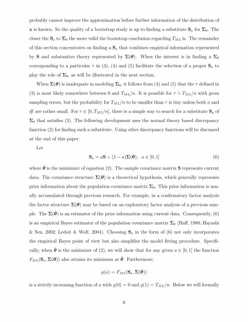
Let

Sa = aS + (1 − a)Σ(θ), a ∈ [0, 1] (6)

where θ is the minimizer of equation (2). The sample covariance matrix S represents current

data. The covariance structure Σ(θ) is a theoretical hypothesis, which generally represents

prior information about the population covariance matrix Σ0. This prior information is usu-

ally accumulated through previous research. For example, in a confirmatory factor analysis

the factor structure Σ(θ) may be based on an exploratory factor analysis of a previous sam-

ple. The Σ(θ) is an estimator of the prior information using current data. Consequently, (6)

is an empirical Bayes estimator of the population covariance matrix Σ0 (Haff, 1980; Hayashi

& Sen, 2002; Ledoit & Wolf, 2004). Choosing Sa in the form of (6) not only incorporates

the empirical Bayes point of view but also simplifies the model fitting procedure. Specifi-

cally, when θ is the minimizer of (2), we will show that for any given a ∈ [0, 1] the function

FML(Sa,Σ(θ)) also attains its minimum at θ. Furthermore,

g(a) = FML(Sa,Σ(θ))

is a strictly increasing function of a with g(0) = 0 and g(1) = TML/n. Below we will formally

6

establish the properties of Sa and FML(Sa,Σ(θ)). We will illustrate how to choose a in the

next section.

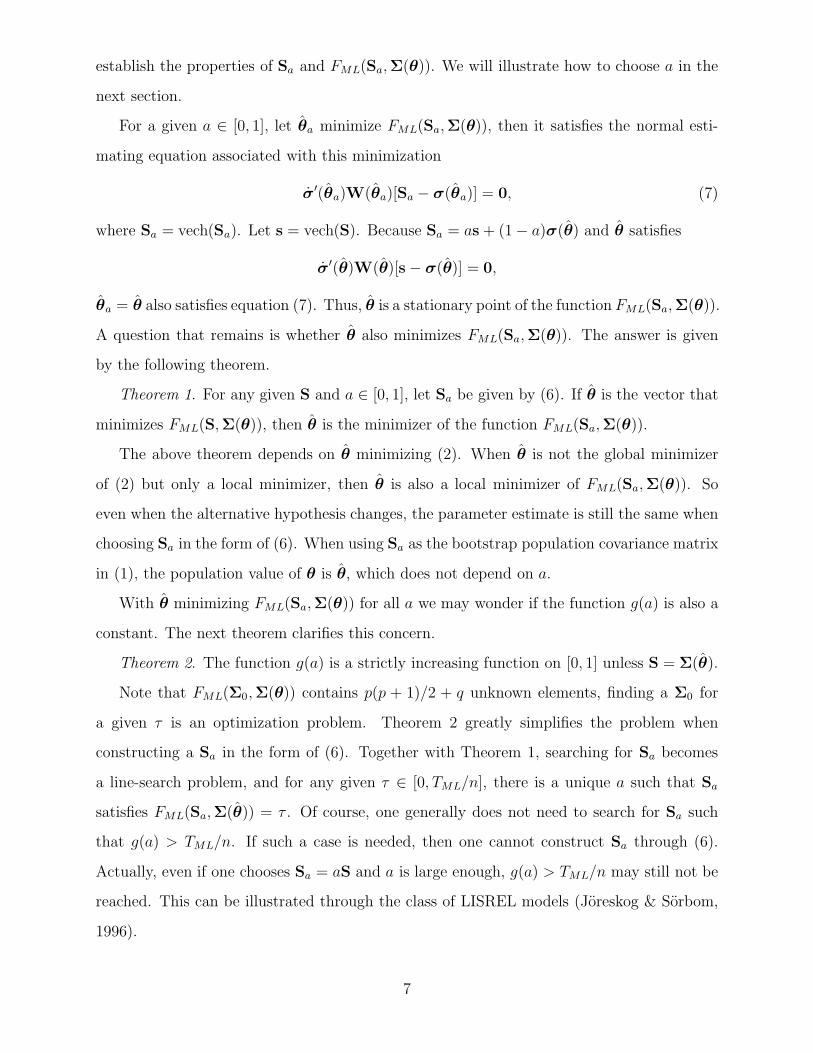
For a given a ∈ [0, 1], let θa minimize FML(Sa,Σ(θ)), then it satisfies the normal esti-

mating equation associated with this minimization

σ′(θa)W(θa)[Sa − σ(θa)] = 0, (7)

where Sa = vech(Sa). Let s = vech(S). Because Sa = as + (1 − a)σ(θ) and θ satisfies

σ′(θ)W(θ)[s − σ(θ)] = 0,

θa = θ also satisfies equation (7). Thus, θ is a stationary point of the function FML(Sa,Σ(θ)).

A question that remains is whether θ also minimizes FML(Sa,Σ(θ)). The answer is given

by the following theorem.

Theorem 1. For any given S and a ∈ [0, 1], let Sa be given by (6). If θ is the vector that

minimizes FML(S,Σ(θ)), then θ is the minimizer of the function FML(Sa,Σ(θ)).

The above theorem depends on θ minimizing (2). When θ is not the global minimizer

of (2) but only a local minimizer, then θ is also a local minimizer of FML(Sa,Σ(θ)). So

even when the alternative hypothesis changes, the parameter estimate is still the same when

choosing Sa in the form of (6). When using Sa as the bootstrap population covariance matrix

in (1), the population value of θ is θ, which does not depend on a.

With θ minimizing FML(Sa,Σ(θ)) for all a we may wonder if the function g(a) is also a

constant. The next theorem clarifies this concern.

Theorem 2. The function g(a) is a strictly increasing function on [0, 1] unless S = Σ(θ).

Note that FML(Σ0,Σ(θ)) contains p(p + 1)/2 + q unknown elements, finding a Σ0 for

a given τ is an optimization problem. Theorem 2 greatly simplifies the problem when

constructing a Sa in the form of (6). Together with Theorem 1, searching for Sa becomes

a line-search problem, and for any given τ ∈ [0, TML/n], there is a unique a such that Sa

satisfies FML(Sa,Σ(θ)) = τ . Of course, one generally does not need to search for Sa such

that g(a) > TML/n. If such a case is needed, then one cannot construct Sa through (6).

Actually, even if one chooses Sa = aS and a is large enough, g(a) > TML/n may still not be

reached. This can be illustrated through the class of LISREL models (Joreskog & Sorbom,

1996).

7

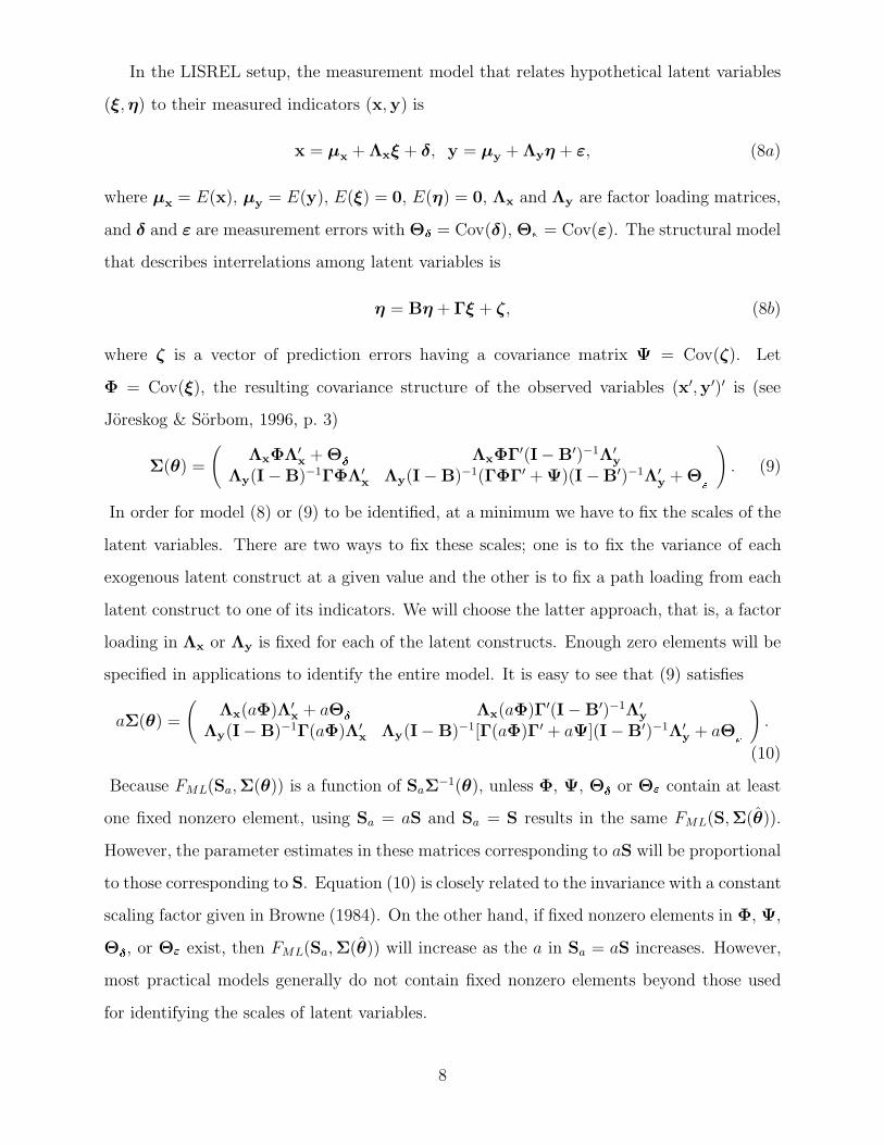
In the LISREL setup, the measurement model that relates hypothetical latent variables

(ξ, η) to their measured indicators (x, y) is

x = μx + Λxξ + δ, y = μy + Λyη + ε, (8a)

where μx = E(x), μy = E(y), E(ξ) = 0, E(η) = 0, Λx and Λy are factor loading matrices,

and δ and ε are measurement errors with ΘÆ = Cov(δ), Θ� = Cov(ε). The structural model

that describes interrelations among latent variables is

η = Bη + Γξ + ζ, (8b)

where ζ is a vector of prediction errors having a covariance matrix Ψ = Cov(ζ). Let

Φ = Cov(ξ), the resulting covariance structure of the observed variables (x′,y′)′ is (see

Joreskog & Sorbom, 1996, p. 3)

Σ(θ) =

(ΛxΦΛ′

x + ΘÆ

ΛxΦΓ′(I− B′)−1Λ′y

Λy(I − B)−1ΓΦΛ′x Λy(I − B)−1(ΓΦΓ′ + Ψ)(I −B′)−1Λ′

y + Θ�

). (9)

In order for model (8) or (9) to be identified, at a minimum we have to fix the scales of the

latent variables. There are two ways to fix these scales; one is to fix the variance of each

exogenous latent construct at a given value and the other is to fix a path loading from each

latent construct to one of its indicators. We will choose the latter approach, that is, a factor

loading in Λx or Λy is fixed for each of the latent constructs. Enough zero elements will be

specified in applications to identify the entire model. It is easy to see that (9) satisfies

aΣ(θ) =

(Λx(aΦ)Λ′

x + aΘÆ

Λx(aΦ)Γ′(I − B′)−1Λ′y

Λy(I− B)−1Γ(aΦ)Λ′x Λy(I− B)−1[Γ(aΦ)Γ′ + aΨ](I− B′)−1Λ′

y + a�

).

(10)

Because FML(Sa,Σ(θ)) is a function of SaΣ−1(θ), unless Φ, Ψ, ΘÆ or Θ� contain at least

one fixed nonzero element, using Sa = aS and Sa = S results in the same FML(S,Σ(θ)).

However, the parameter estimates in these matrices corresponding to aS will be proportional

to those corresponding to S. Equation (10) is closely related to the invariance with a constant

scaling factor given in Browne (1984). On the other hand, if fixed nonzero elements in Φ, Ψ,

ΘÆ, or Θ� exist, then FML(Sa,Σ(θ)) will increase as the a in Sa = aS increases. However,

most practical models generally do not contain fixed nonzero elements beyond those used

for identifying the scales of latent variables.

8

More generally, when one chooses Sακ = αS + κΣ(θ) for positive numbers α and κ, Sακ

can be rewritten as

Sακ = b[aS + (1 − a)Σ(θ)] = bSa,

where b = (α +κ) and a = α/(α +κ). Suppose the covariance structure Σ(θ) is represented

by (9) and there are no fixed nonzero elements beyond those for identification purposes. It

follows from (10) that, corresponding to each θ minimizing FML(S,Σ(θ)), there always exists

a θ∗

that minimizes FML(Sακ,Σ(θ)) with the same minimum as that of FML(Sa,Σ(θ)). This

implies that it is impossible to find a Sακ to reach a τ > TML/n. Actually, a Sa corresponding

to a τ > TML/n sits most likely farther than τ away from the model Σ(θ).

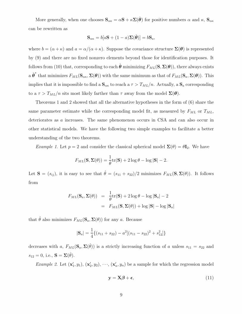
Theorems 1 and 2 showed that all the alternative hypotheses in the form of (6) share the

same parameter estimate while the corresponding model fit, as measured by FML or TML,

deteriorates as a increases. The same phenomenon occurs in CSA and can also occur in

other statistical models. We have the following two simple examples to facilitate a better

understanding of the two theorems.

Example 1. Let p = 2 and consider the classical spherical model Σ(θ) = θI2. We have

FML(S,Σ(θ)) =1

θtr(S) + 2 log θ − log |S| − 2.

Let S = (sij), it is easy to see that θ = (s11 + s22)/2 minimizes FML(S,Σ(θ)). It follows

from

FML(Sa,Σ(θ)) =1

θtr(S) + 2 log θ − log |Sa| − 2

= FML(S,Σ(θ)) + log |S| − log |Sa|

that θ also minimizes FML(Sa,Σ(θ)) for any a. Because

|Sa| =1

4{(s11 + s22) − a2[(s11 − s22)

2 + s212]}

decreases with a, FML(Sa,Σ(θ)) is a strictly increasing function of a unless s11 = s22 and

s12 = 0, i.e., S = Σ(θ).

Example 2. Let (x′1, y1), (x′

2, y2), · · ·, (x′n, yn) be a sample for which the regression model

y = Xβ + ε, (11)

9

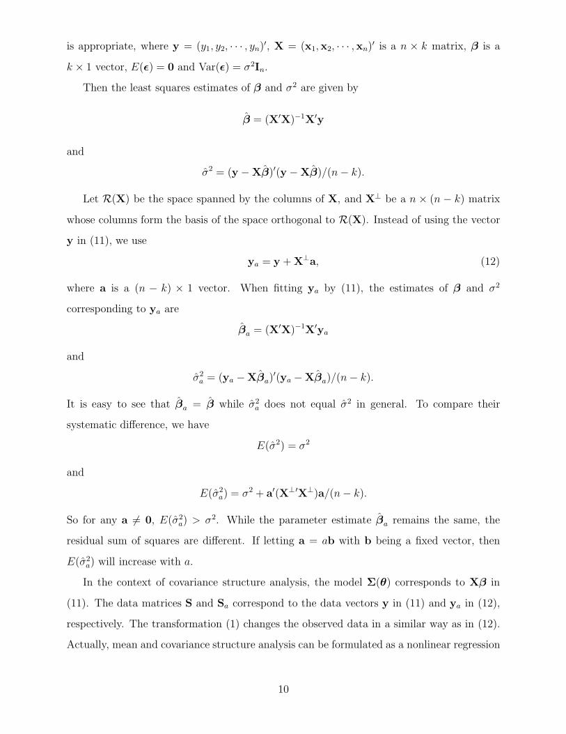
is appropriate, where y = (y1, y2, · · · , yn)′, X = (x1,x2, · · · ,xn)

′ is a n × k matrix, β is a

k × 1 vector, E(ε) = 0 and Var(ε) = σ2In.

Then the least squares estimates of β and σ2 are given by

β = (X′X)−1X′y

and

σ2 = (y − Xβ)′(y − Xβ)/(n − k).

Let R(X) be the space spanned by the columns of X, and X⊥ be a n × (n − k) matrix

whose columns form the basis of the space orthogonal to R(X). Instead of using the vector

y in (11), we use

ya = y + X⊥a, (12)

where a is a (n − k) × 1 vector. When fitting ya by (11), the estimates of β and σ2

corresponding to ya are

βa = (X′X)−1X′ya

and

σ2a = (ya −Xβa)

′(ya − Xβa)/(n − k).

It is easy to see that βa = β while σ2a does not equal σ2 in general. To compare their

systematic difference, we have

E(σ2) = σ2

and

E(σ2a) = σ2 + a′(X⊥′X⊥)a/(n− k).

So for any a �= 0, E(σ2a) > σ2. While the parameter estimate βa remains the same, the

residual sum of squares are different. If letting a = ab with b being a fixed vector, then

E(σ2a) will increase with a.

In the context of covariance structure analysis, the model Σ(θ) corresponds to Xβ in

(11). The data matrices S and Sa correspond to the data vectors y in (11) and ya in (12),

respectively. The transformation (1) changes the observed data in a similar way as in (12).

Actually, mean and covariance structure analysis can be formulated as a nonlinear regression

10

model (Browne, 1982; Lee & Jennrich, 1984; Yuan & Bentler, 1997). Unfortunately, in the

context of nonlinear models there does not exist a clean formula as in the context of linear

regression models.

3. Illustrations

We will illustrate how to choose a proper Sa in (6). There are two circumstances that

particular covariance matrices are needed. One is to study the behavior of TML or a fit index

for a given sample under certain degree of misspecification. The degree of misspecification is

typically quantified by the τ in (3). The other is to study the behavior of TML or a fit index

for a given sample when Σ0 or the τ in (3) is unknown. Because τ can only be estimated,

we can only obtain a substitute for Σ0 in the later case. We will illustrate the two cases by

the following example.

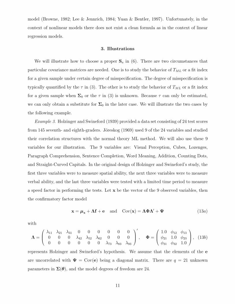
Example 3. Holzinger and Swineford (1939) provided a data set consisting of 24 test scores

from 145 seventh- and eighth-graders. Joreskog (1969) used 9 of the 24 variables and studied

their correlation structures with the normal theory ML method. We will also use these 9

variables for our illustration. The 9 variables are: Visual Perception, Cubes, Lozenges,

Paragraph Comprehension, Sentence Completion, Word Meaning, Addition, Counting Dots,

and Straight-Curved Capitals. In the original design of Holzinger and Swineford’s study, the

first three variables were to measure spatial ability, the next three variables were to measure

verbal ability, and the last three variables were tested with a limited time period to measure

a speed factor in performing the tests. Let x be the vector of the 9 observed variables, then

the confirmatory factor model

x = μx + Λf + e and Cov(x) = ΛΦΛ′ + Ψ (13a)

with

Λ =

⎛⎜⎝ λ11 λ21 λ31 0 0 0 0 0 0

0 0 0 λ42 λ52 λ62 0 0 00 0 0 0 0 0 λ73 λ83 λ93

⎞⎟⎠

′

, Φ =

⎛⎜⎝ 1.0 φ12 φ13

φ21 1.0 φ23

φ31 φ32 1.0

⎞⎟⎠ , (13b)

represents Holzinger and Swineford’s hypothesis. We assume that the elements of the e

are uncorrelated with Ψ = Cov(e) being a diagonal matrix. There are q = 21 unknown

parameters in Σ(θ), and the model degrees of freedom are 24.

11

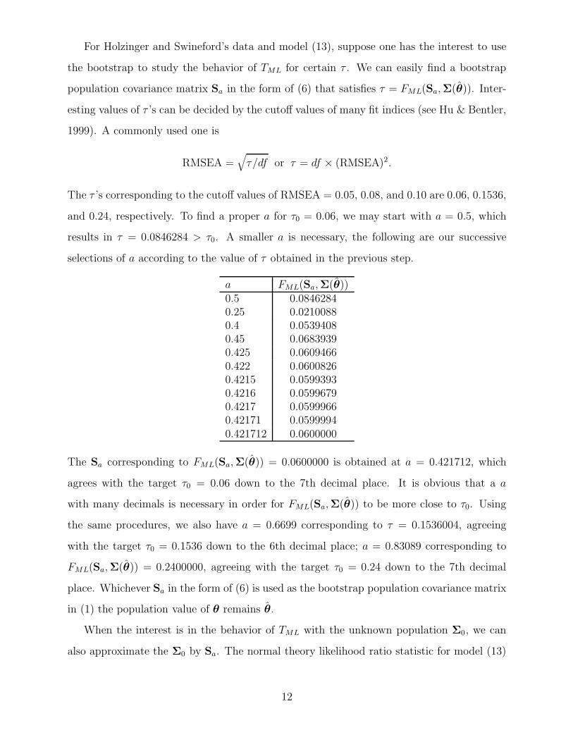
For Holzinger and Swineford’s data and model (13), suppose one has the interest to use

the bootstrap to study the behavior of TML for certain τ . We can easily find a bootstrap

population covariance matrix Sa in the form of (6) that satisfies τ = FML(Sa,Σ(θ)). Inter-

esting values of τ ’s can be decided by the cutoff values of many fit indices (see Hu & Bentler,

1999). A commonly used one is

RMSEA =√

τ/df or τ = df × (RMSEA)2.

The τ ’s corresponding to the cutoff values of RMSEA = 0.05, 0.08, and 0.10 are 0.06, 0.1536,

and 0.24, respectively. To find a proper a for τ0 = 0.06, we may start with a = 0.5, which

results in τ = 0.0846284 > τ0. A smaller a is necessary, the following are our successive

selections of a according to the value of τ obtained in the previous step.

a FML(Sa,Σ(θ))0.5 0.08462840.25 0.02100880.4 0.05394080.45 0.06839390.425 0.06094660.422 0.06008260.4215 0.05993930.4216 0.05996790.4217 0.05999660.42171 0.05999940.421712 0.0600000

The Sa corresponding to FML(Sa,Σ(θ)) = 0.0600000 is obtained at a = 0.421712, which

agrees with the target τ0 = 0.06 down to the 7th decimal place. It is obvious that a a

with many decimals is necessary in order for FML(Sa,Σ(θ)) to be more close to τ0. Using

the same procedures, we also have a = 0.6699 corresponding to τ = 0.1536004, agreeing

with the target τ0 = 0.1536 down to the 6th decimal place; a = 0.83089 corresponding to

FML(Sa,Σ(θ)) = 0.2400000, agreeing with the target τ0 = 0.24 down to the 7th decimal

place. Whichever Sa in the form of (6) is used as the bootstrap population covariance matrix

in (1) the population value of θ remains θ.

When the interest is in the behavior of TML with the unknown population Σ0, we can

also approximate the Σ0 by Sa. The normal theory likelihood ratio statistic for model (13)

12

is TML = 51.543 and is highly significant when referring to χ224. If assuming TML ∼ χ2

24(δ)

with δ = nτ and τ = FML(Σ0,Σ(θ∗)), then the commonly used estimate of τ is given by

τ1 = (TML − 24)/n = 0.1899509. Using essentially the same procedure for finding a Sa

corresponding to a given RMSEA, we have a = 0.74259 corresponding to FML(Sa,Σ(θ)) =

0.1899506, which agrees with τ1 down to the 6th decimal place.

The statistic TML is derived from x ∼ N(μ0,Σ0). Other test statistics that do not assume

the normal distribution of the data also imply that the model does not fit the data well. It is

more natural to regard the Σ0 as a fixed covariance matrix for Holzinger and Swineford’s data

rather than changing with n. Thus, an estimate of τ based on (5) should be more reasonable.

Using S to estimate Σ0, θ to estimate θ∗, and denoting yi = vech[(xi − x)(xi − x)′] and

using the sample covariance matrix Sy of yi to estimate Π, we have tr(UΠ) = 22.873261

and τ2 = [TML − tr(UΠ)]/n = 0.1977215. Now we can approximate Σ0 by Sa in (6). The

a = 0.757098 corresponds to FML(Sa,Σ(θ)) = 0.1977214, agreeing with τ2 to the 6th decimal

place.

Once τ or τ is known, the search for Sa, as illustrated above, can be performed using any

standard SEM program (e.g., Bentler, 2006) that allows the printing of FML(S,Σ(θ)) and

Σ(θ) down to several decimals. The calculation of Sa in (6) can be done by any software

that contains the functions of matrix addition and multiplication (e.g., SAS IML, Matlab,

Splus). The estimation of τ based on (5) involves second derivatives of Σ(θ) with respect to

θ, which is usually quite complicated and not any SEM program provides its calculation at

present.

4. Conclusion and Discussion

A covariance structure model in practice is, at best, only an approximation to Σ0, there

should be a great interest in studying the behavior of a statistic when τ > 0 (see MacCallum,

Browne & Sugawara, 1996). With unknown distributions of x in practice, the bootstrap

remains a valuable tool for such studies. Because the behavior of any statistic T is closely

related to Σ0, when Σ0 is unknown, finding a Sa that approximately equals Σ0 allows us to

obtain more accurate evaluation of TML. The purpose of the paper is to provide the class

of covariance matrices represented by Sa = aS + (1 − a)Σ(θ). The nice properties of Sa

13

make it an ideal choice for playing the role of the bootstrap population covariance matrix.

Example 3 shows that it is straightforward to find a proper Sa once the τ or its estimate is

given. Specific applications of Sa in bootstrap simulation were given in Yuan and Hayashi

(2003).

When using Sa to approximate the unknown Σ0, the quality of the approximation de-

pends on S as well as the goodness of the model Σ(θ). When the sample size n is small or

when the distribution of x is of heavy tails, S may not be a good estimate of Σ0 even it is

unbiased, the τ1 or τ2 in the previous section can be a poor estimate of τ . It is possible that

τ1 or τ2 may be negative even when τ > 0, then we might have to estimate Σ0 by S0 = Σ(θ).

Although the form of Sa in (6) combines both theory and empirical data, it can still be quite

different from the true Σ0. But such obtained Sa, especially the one corresponding to τ2,

should be more close to Σ0 than those obtained previously in the literature where no effort

was made in approximating the true Σ0. Of course, when Σ0 is known or a better estimator

of Σ0 than that given in (6) is available, then such a covariance matrix should be used in

the transformation (1) for more accurate bootstrap inference.

We have focused on using the normal theory based discrepancy function (2) to establish

the properties of Sa in section 2. One may wonder if similar properties can be established for

other types of discrepancy functions. In covariance structure analysis, a very general form

of discrepancy function is (see Shapiro, 1985)

F (S,Σ(θ)) = [s− σ(θ)]′W[s− σ(θ)]

for a proper weight matrix W. It can be verified directly that, when W is only a function of

θ or a constant matrix, F (Sa,Σ(θ)) will enjoy the same properties of FML(Sa,Σ(θ)) as in

Theorems 1 and 2. Special cases are the normal theory based likelihood discrepancy function

and the least squares discrepancy function. However, when W involves x(a)i the properties

in Theorems 1 and 2 may no longer apply to F (Sa,Σ(θ)). A special case for this is when

W = (S(a)y )−1, where S(a)

y is the sample covariance matrix of y(a)i = vech[(x

(a)i −xa)(x

(a)i −xa)

′]

with xa =∑n

i=1 x(a)i /n. Comparing several commonly used discrepancy functions for power

analysis, Yuan and Hayashi (2003) showed that, with a proper downweighting of heavy tails,

the bootstrap based on the normal theory discrepancy function in (2) leads to the most

14

powerful test for covariance structure analysis.

Because a covariance structure Σ(θ) represents prior information about the population

covariance matrix, we propose to use the Sa in (6) to estimate the population covariance

matrix. When no such information is available, the form Sab = aS + bI has been shown to

enjoy some nice properties with respect to several loss functions (Efron & Morris, 1976; Haff,

1980). It is also interesting to study properties of Sa with respect to some loss functions and

to find a proper prior distribution to formally justify its Bayes nature.

Standard errors in CSA are also affected by model misspecification (Yuan & Hayashi, in

press). Because different Sa’s correspond to the same θ, choosing a bootstrap population

covariance matrix in the form of Sa in (6) will facilitate the study of standard error changes

with varying degree of model misspecification.

We have mainly discussed the candidacy of Sa in playing the role of the bootstrap popu-

lation covariance matrix. It can also be used as the population covariance matrix in Monte

Carlo studies. Since the behavior of a statistic is closely related to Σ0 (Yuan et al., 2005),

a Σ0 that reflects the reality will enhance the validity of the conclusion of a Monte Carlo

study. Most previous Monte Carlo studies constructed Σ0 according to certain structures

while the models are created by omitting or fixing a subset of parameters in θ. Such created

model misspecifications might be interesting but may not be realistic. The Sa in (6) should

better reflect the fact that “All models are wrong but some are useful.” (Box, 1979).

Appendix

Proof of Theorem 1: It is obvious that θ minimizes FML(Sa,Σ(θ)) when a = 0 or 1. For

a general a ∈ [0, 1] we can rewrite FML(Sa,Σ(θ)) as

FML(Sa,Σ(θ)) = atr[SΣ−1(θ)] + (1 − a)tr[Σ(θ)Σ−1(θ)] − ln |Σ(θ)Σ−1(θ)| − p

+ ln[|Σ(θ)Σ−1(θ)|/|aSΣ−1(θ) + (1 − a)Σ(θ)Σ−1(θ)|]

= atr[(S − Σ(θ))Σ−1(θ)] + FML(Σ(θ),Σ(θ))

+ ln[|Σ(θ)|/|aS + (1 − a)Σ(θ)|].

(A1)

15

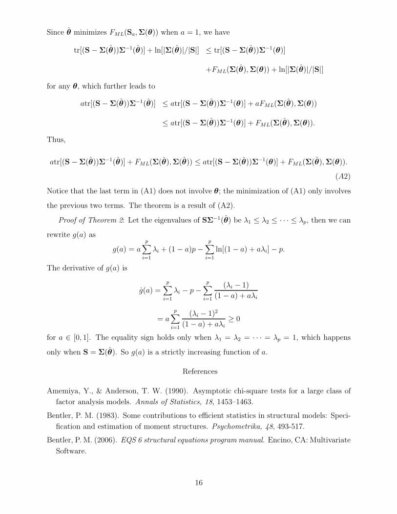
Since θ minimizes FML(Sa,Σ(θ)) when a = 1, we have

tr[(S − Σ(θ))Σ−1(θ)] + ln[|Σ(θ)|/|S|] ≤ tr[(S −Σ(θ))Σ−1(θ)]

+FML(Σ(θ),Σ(θ)) + ln[|Σ(θ)|/|S|]for any θ, which further leads to

atr[(S− Σ(θ))Σ−1(θ)] ≤ atr[(S − Σ(θ))Σ−1(θ)] + aFML(Σ(θ),Σ(θ))

≤ atr[(S − Σ(θ))Σ−1(θ)] + FML(Σ(θ),Σ(θ)).

Thus,

atr[(S −Σ(θ))Σ−1(θ)] + FML(Σ(θ),Σ(θ)) ≤ atr[(S − Σ(θ))Σ−1(θ)] + FML(Σ(θ),Σ(θ)).

(A2)

Notice that the last term in (A1) does not involve θ; the minimization of (A1) only involves

the previous two terms. The theorem is a result of (A2).

Proof of Theorem 2: Let the eigenvalues of SΣ−1(θ) be λ1 ≤ λ2 ≤ · · · ≤ λp, then we can

rewrite g(a) as

g(a) = ap∑

i=1

λi + (1 − a)p −p∑

i=1

ln[(1 − a) + aλi] − p.

The derivative of g(a) is

g(a) =p∑

i=1

λi − p −p∑

i=1

(λi − 1)

(1 − a) + aλi

= ap∑

i=1

(λi − 1)2

(1 − a) + aλi≥ 0

for a ∈ [0, 1]. The equality sign holds only when λ1 = λ2 = · · · = λp = 1, which happens

only when S = Σ(θ). So g(a) is a strictly increasing function of a.

References

Amemiya, Y., & Anderson, T. W. (1990). Asymptotic chi-square tests for a large class of

factor analysis models. Annals of Statistics, 18, 1453–1463.

Bentler, P. M. (1983). Some contributions to efficient statistics in structural models: Speci-

fication and estimation of moment structures. Psychometrika, 48, 493-517.

Bentler, P. M. (2006). EQS 6 structural equations program manual. Encino, CA: Multivariate

Software.

16

Bentler, P. M., & Dijkstra, T. K. (1985). Efficient estimation via linearization in structural

models. In P. R. Krishnaiah (Ed.), Multivariate analysis VI (pp. 9–42). Amsterdam:

North-Holland.

Bentler, P. M., & Dudgeon, P. (1996). Covariance structure analysis: Statistical practice,

theory, directions. Annual Review of Psychology, 47, 563–592.

Bentler, P. M., & Yuan, K.-H. (1999). Structural equation modeling with small samples:

Test statistics. Multivariate Behavioral Research, 34, 181–197.

Beran, R. (1986). Simulated power functions. Annals of Statistics, 14, 151–173.

Beran, R., & Srivastava, M. S. (1985). Bootstrap tests and confidence regions for functions

of a covariance matrix. Annals of Statistics, 13, 95–115.

Bollen, K. A. (2002). Latent variables in psychology and the social sciences. Annual Review

of Psychology, 53, 605–634.

Bollen, K. A., & Stine, R. (1990). Direct and indirect effects: Classical and bootstrap

estimates of variability. In C. C. Clogg (Ed.), Sociological methodology 1990 (pp. 115–

140). Oxford: Basil Blackwell.

Bollen, K. A., & Stine, R. (1993). Bootstrapping goodness of fit measures in structural

equation models. In K. A. Bollen & J. S. Long (Eds.), Testing structural equation models

(pp. 111–135). Newbury Park, CA: Sage.

Boomsma, A. (1986). On the use of bootstrap and jackknife in covariance structure analysis.

Compstat 1986, 205–210.

Box, G. E. P. (1979). Robustness in the strategy of scientific model building. In R. L. Launer

& G. N. Wilkinson (Eds.), Robustness in statistics (pp. 201–236). New York: Academic

Press

Browne, M. W. (1982). Covariance structure analysis. In D. M. Hawkins (Ed.), Topics in

applied multivariate analysis (pp. 72–141). Cambridge: Cambridge University Press.

Browne, M. W. (1984). Asymptotic distribution-free methods for the analysis of covariance

structures. British Journal of Mathematical and Statistical Psychology, 37, 62–83.

Browne, M. W., & Shapiro, A. (1988). Robustness of normal theory methods in the analysis

of linear latent variate models. British Journal of Mathematical and Statistical Psychology,

41, 193–208.

Chatterjee, S. (1984). Variance estimation in factor analysis: An application of the boot-

strap. British Journal of Mathematical and Statistical Psychology, 37, 252–262.

Chou, C.-P., Bentler, P. M., & Satorra, A. (1991). Scaled test statistics and robust standard

errors for nonnormal data in covariance structure analysis: A Monte Carlo study. British

Journal of Mathematical and Statistical Psychology, 44, 347–357.

17

Cudeck, R., & Browne, M. W. (1992). Constructing a covariance matrix that yields a

specified minimizer and a specified minimum discrepancy function value. Psychometrika,

57, 357–369.

Curran, P. S., West, S. G., & Finch, J. F. (1996). The robustness of test statistics to non-

normality and specification error in confirmatory factor analysis. Psychological Methods,

1, 16–29.

Davison, A. C., & Hinkley, D. V. (1997). Bootstrap methods and their applications. Cam-

bridge: Cambridge University Press.

Efron, B. (1979). Bootstrap methods: Another look at the jackknife. Annals of Statistics,

7, 1–26.

Efron, B., & Morris, C. (1976). Multivariate empirical Bayes and estimation of covariance

matrices. Annals of Statistics, 4, 22–32.

Efron, B., & Tibshirani, R. J. (1993). An introduction to the bootstrap. New York: Chapman

& Hall.

Enders, C.K. (2002). Applying the Bollen-Stine bootstrap for goodness-of-fit measures to

structural equation models with missing data. Multivariate Behavioral Research, 37, 359–

377.

Fouladi, R. T. (2000). Performance of modified test statistics in covariance and correlation

structure analysis under conditions of multivariate nonnormality. Structural Equation

Modeling, 7, 356–410.

Haff, L. R. (1980). Empirical Bayes estimation of the multivariate normal covariance matrix.

Annals of Statistics, 8, 586–597.

Hall, P., & Titterington, D. M. (1989). The effect of simulation order on level accuracy

and power of Monte Carlo tests. Journal of the Royal Statistical Society. Series B, 51,

459–467.

Hayashi, K., & Sen, P. K. (2002). Bias-corrected estimator of factor loadings in Bayesian

factor analysis. Educational and Psychological Measurement, 62, 944–959.

Holzinger, K. J., & Swineford, F. (1939). A study in factor analysis: The stability of a

bi-factor solution. University of Chicago: Supplementary Educational Monographs, No.

48.

Hu, L., & Bentler, P. M. (1999). Cutoff criteria for fit indexes in covariance structure

analysis: Conventional criteria versus new alternatives. Structural Equation Modeling, 6,

1–55.

Hu, L., Bentler, P. M., & Kano, Y. (1992). Can test statistics in covariance structure analysis

be trusted? Psychological Bulletin, 112, 351–362.

Joreskog, K. G. (1969). A general approach to confirmatory maximum likelihood factor

18

analysis. Psychometrika, 34, 183–202.

Joreskog, K. G., & Sorbom, D. (1996). LISREL 8 user’s reference guide. Chicago: Scientific

Software International.

Kano, Y., Berkane, M., & Bentler, P. M. (1990). Covariance structure analysis with hetero-

geneous kurtosis parameters. Biometrika, 77, 575–585.

Ledoit, O., & Wolf, M. (2004). A well-conditioned estimator for large-dimensional covariance

matrices. Journal of Multivariate Analysis, 88, 365–411.

Lee, S.-Y., & Jennrich, R. I. (1984). The analysis of structural equation models by means

of derivative free nonlinear least squares. Psychometrika, 49, 521–528.

MacCallum, R. C., Browne, M. W. & Sugawara, H. M. (1996). Power analysis and de-

termination of sample size for covariance structure modeling. Psychological Methods, 1,

130–149.

MacCallum, R. C., & Austin, J. T. (2000). Applications of structural equation modeling in

psychological research. Annual Review of Psychology, 51, 201–226.

Magnus, J. R., & Neudecker, H. (1999). Matrix differential calculus with applications in

statistics and econometrics. New York: Wiley.

Muthen, B., & Kaplan, D. (1985). A comparison of some methodologies for the factor

analysis of non-normal Likert variables. British Journal of Mathematical and Statistical

Psychology, 38, 171–189.

Satorra, A. (1989). Alternative test criteria in covariance structure analysis: A unified

approach. Psychometrika, 54, 131–151.

Satorra, A., & Bentler, P. M. (1994). Corrections to test statistics and standard errors

in covariance structure analysis. In A. von Eye & C. C. Clogg (Eds.), Latent variables

analysis: Applications for developmental research (pp. 399-419). Newbury Park, CA:

Sage.

Satorra, A., & Saris, W. E. (1985). Power of the likelihood ratio test in covariance structure

analysis. Psychometrika, 50, 83–90.

Shapiro, A. (1983). Asymptotic distribution theory in the analysis of covariance structures

(a unified approach). South African Statistical Journal, 17, 33–81.

Shapiro, A. (1985). Asymptotic equivalence of minimum discrepancy function estimators to

GLS estimators. South African Statistical Journal, 19, 73–81.

Shapiro, A., & Browne, M. W. (1987). Analysis of covariance structures under elliptical

distributions. Journal of the American Statistical Association, 82, 1092–1097.

Steiger, J. H., & Lind, J. M. (1980). Statistically based tests for the number of common

factors. Paper presented at the annual meeting of the Psychometric Society. Iowa City,

19

IA.

Steiger, J. H., Shapiro, A., & Browne, M. W. (1985). On the multivariate asymptotic

distribution of sequential chi-square statistics. Psychometrika, 50, 253–264.

Yuan, K.-H. (2005). Fit indices versus test statistics. Multivariate Behavioral Research, 40,

115–148.

Yuan, K.-H., & Bentler, P. M. (1997). Mean and covariance structure analysis: Theoretical

and practical improvements. Journal of the American Statistical Association, 92, 767–774.

Yuan, K.-H., & Bentler, P. M. (1998). Normal theory based test statistics in structural

equation modeling. British Journal of Mathematical and Statistical Psychology, 51, 289–

309.

Yuan, K.-H., & Bentler, P. M. (1999a). F-tests for mean and covariance structure analysis.

Journal of Educational and Behavioral Statistics, 24, 225–243.

Yuan, K.-H., & Bentler, P. M. (1999b). On normal theory and associated test statistics

in covariance structure analysis under two classes of nonnormal distributions. Statistica

Sinica, 9, 831–853.

Yuan, K.-H., & Hayashi, K. (2003). Bootstrap approach to inference and power analysis

based on three test statistics for covariance structure models. British Journal of Mathe-

matical and Statistical Psychology, 56, 93–110.

Yuan, K.-H., & Hayashi, K. (in press). Standard errors in covariance structure models:

Asymptotics versus bootstrap. British Journal of Mathematical and Statistical Psychol-

ogy.

Yuan, K.-H., Hayashi, K., & Bentler, P. M. (2005). Normal theory likelihood ratio statistic

for mean and covariance structure analysis under alternative hypotheses. Under review.

Yuan, K.-H., & Marshall, L. L. (2004). A new measure of misfit for covariance structure

models. Behaviormetrika, 31, 67–90.

Yung, Y. F., & Bentler, P. M. (1996). Bootstrapping techniques in analysis of mean and

covariance structures. In G. A. Marcoulides & R. E. Schumacker (Eds.), Advanced struc-

tural equation modeling: Techniques and issues (pp. 195–226). Hillsdale, New Jersey:

Lawrence Erlbaum.

20