Embed Size (px)
Citation preview
Universita degli Studi “Roma Tre”
Dottorato di Ricerca in Matematica
A class of Phase Transition problems
with the Line Tension effect
Direttore di tesi Dottorando
Chiar.ma Prof.ssa Adriana Garroni Giampiero PalatucciCoordinatore del Dottorato
Chiar.mo Prof. Renato Spigler
XVIII Ciclo
Ringrazio il mio direttore di tesi Adriana Garroni per tutti gli insegnamenti che da lei
ho tratto e per l’entusiasmo e la pazienza con cui mi ha accompagnato in questi anni.
Ringrazio tutte le persone con cui ho collaborato all’Universita di “Roma Tre” e
all’Universita “La Sapienza” di Roma; in particolare Caterina Zeppieri, Adriano Pisante,
Francesco Petitta, Marcello Ponsiglione e Tommaso Leonori. Da loro ho imparato molte
cose e condividiamo la grande passione per la matematica che ci ha unito in una bella
amicizia. Ringrazio Enrico Valdinoci per l’interesse mostrato nel mio lavoro e per le utili
discussioni.
Ringrazio l’ospitalita del Centro di Ricerca Matematica “Ennio De Giorgi” di Pisa,
dove ho scritto l’ultima parte di questa tesi e dove ho avuto modo di riflettere su interes-
santi problemi con Gianluca Crippa e Marco Barchiesi.
Grazie ai miei amici Marco, Isabella e Mariapia, e ai miei fratelli Luca e Mauro, che,
ognuno a suo modo, sono stati presenti durante tutti questi anni di Dottorato.
Questa tesi non sarebbe potuta esistere senza il supporto e l’incoraggiamento dei miei
genitori e di Iside, che mi hanno sostenuto con amore sin dal primo momento.
Giampiero Palatucci


Contents
Introduction . . . . . . . . . . . . . . . . . . . . . . . . . . . . . . . . . . . 6
1 Preliminaries 18
1.1 Γ-Convergence . . . . . . . . . . . . . . . . . . . . . . . . . . . . . . . . . 19
1.1.1 Choice of interesting rescalings . . . . . . . . . . . . . . . . . . . . 21
1.2 Young Measures . . . . . . . . . . . . . . . . . . . . . . . . . . . . . . . . 21
1.2.1 The fundamental theorem on Young measures and applications . . 22
1.3 The slicing method . . . . . . . . . . . . . . . . . . . . . . . . . . . . . . . 24
1.3.1 Some slicing results . . . . . . . . . . . . . . . . . . . . . . . . . . 26
1.3.2 Isometry defect . . . . . . . . . . . . . . . . . . . . . . . . . . . . . 27
1.4 Rearrangement results . . . . . . . . . . . . . . . . . . . . . . . . . . . . . 29
1.4.1 Monotone rearrangement in one-dimension . . . . . . . . . . . . . 29
1.4.2 Monotone rearrangement in one direction . . . . . . . . . . . . . . 31
2 Phase transitions and known results 32
2.1 The classical model for phase transitions . . . . . . . . . . . . . . . . . . . 32
2.2 The Cahn-Hilliard model for phase transitions . . . . . . . . . . . . . . . . 33
2.3 The Modica-Mortola Theorem . . . . . . . . . . . . . . . . . . . . . . . . 34
2.4 The interactions between the fluids and the wall of the container . . . . . 37
2.5 Phase transitions with line tension effect . . . . . . . . . . . . . . . . . . . 39
3 A singular perturbation result with a fractional norm 44
3.1 The Γ-convergence result . . . . . . . . . . . . . . . . . . . . . . . . . . . 45
3.2 The optimal profile problem . . . . . . . . . . . . . . . . . . . . . . . . . . 46
3.3 Compactness . . . . . . . . . . . . . . . . . . . . . . . . . . . . . . . . . . 51
3.4 Lower bound inequality . . . . . . . . . . . . . . . . . . . . . . . . . . . . 54
3.5 Upper bound inequality . . . . . . . . . . . . . . . . . . . . . . . . . . . . 58
4
CONTENTS
4 A class of phase transition problems with line tension effect 60
4.1 Strategy of the proof and some preliminary results . . . . . . . . . . . . . 63
4.1.1 The bulk effect . . . . . . . . . . . . . . . . . . . . . . . . . . . . . 63
4.1.2 The wall effect . . . . . . . . . . . . . . . . . . . . . . . . . . . . . 63
4.1.3 The boundary effect . . . . . . . . . . . . . . . . . . . . . . . . . . 68
4.2 Some remark about the structure of Fε . . . . . . . . . . . . . . . . . . . . 69
5 Recovering the “contribution of the wall”: the flat case 72
5.1 Compactness of the traces . . . . . . . . . . . . . . . . . . . . . . . . . . . 73
5.2 Lower bound inequality . . . . . . . . . . . . . . . . . . . . . . . . . . . . 74
5.3 Reduction to the flat case . . . . . . . . . . . . . . . . . . . . . . . . . . . 78
5.4 Existence of an optimal profile problem . . . . . . . . . . . . . . . . . . . 81
6 Proof of the main result 87
6.1 Compactness . . . . . . . . . . . . . . . . . . . . . . . . . . . . . . . . . . 88
6.2 Lower bound inequality . . . . . . . . . . . . . . . . . . . . . . . . . . . . 88
6.3 Upper bound inequality . . . . . . . . . . . . . . . . . . . . . . . . . . . . 91
List of Symbols 100
List of Figures 102
Bibliography 103
5
INTRODUCTION
Introduction
In this thesis we study a class of problems concerning the analysis of liquid-liquid phase
transitions, from a variational point of view. In the literature, there are many variants of
functionals of the Calculus of Variation, describing phase transitions phenomena.
We now give a brief overview of the iter that brings us through the choice of this class
of problems.
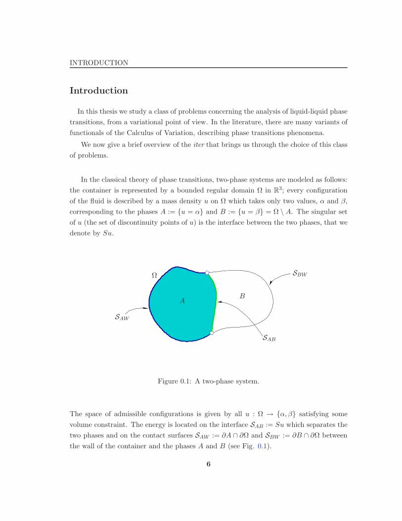
In the classical theory of phase transitions, two-phase systems are modeled as follows:
the container is represented by a bounded regular domain Ω in R3; every configuration
of the fluid is described by a mass density u on Ω which takes only two values, α and β,
corresponding to the phases A := u = α and B := u = β = Ω \ A. The singular set
of u (the set of discontinuity points of u) is the interface between the two phases, that we
denote by Su.
Ω
SAB
SBW
SAW
AB
Figure 0.1: A two-phase system.
The space of admissible configurations is given by all u : Ω → α, β satisfying some
volume constraint. The energy is located on the interface SAB := Su which separates the
two phases and on the contact surfaces SAW := ∂A ∩ ∂Ω and SBW := ∂B ∩ ∂Ω between
the wall of the container and the phases A and B (see Fig. 0.1).
6
INTRODUCTION
Hence, the equilibrium configurations are assumed to minimize the capillary energy
E0(A) := σH2(SAB) + σAWH2(SAW ) + σBWH2(SBW ), (0.1)
where Hk denotes the k-dimensional Hausdorff measure. The positive constants σ, σAW ,
σBW in (0.1) are referred to as surface tensions.
In the late 50’s, Cahn and Hilliard [24] proposed an alternative way to study two-
phase fluids. They followed the continuum mechanics approach by Gibbs and assumed
that the transition is not given by a separating interface, but is a continuous phenomenon
occurring in a thin layer which, on a macroscopic level, is identified with the interface. In
this region, a fine mixture of the two-phases fluid is allowed.
Hence, a configuration of the system is described by a mass density u which varies con-
tinuously from the value α to the value β, under a suitable volume constraint.
α β
W
x
Figure 0.2: A double-well type potential W .
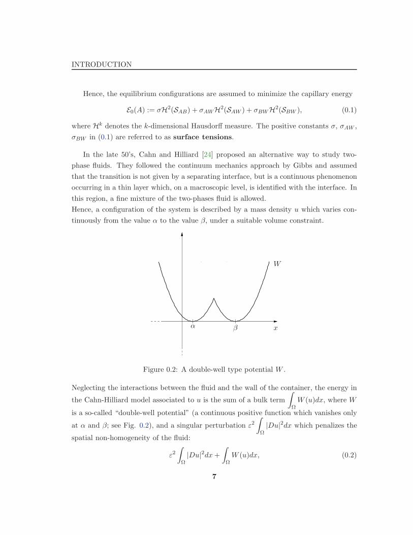
Neglecting the interactions between the fluid and the wall of the container, the energy in
the Cahn-Hilliard model associated to u is the sum of a bulk term
∫
ΩW (u)dx, where W
is a so-called “double-well potential” (a continuous positive function which vanishes only
at α and β; see Fig. 0.2), and a singular perturbation ε2∫
Ω|Du|2dx which penalizes the
spatial non-homogeneity of the fluid:
ε2∫
Ω|Du|2dx+
∫
ΩW (u)dx, (0.2)
7
INTRODUCTION
where ε is a small parameter, giving the characteristic length of the thickness of the
interface. This model is also known as “diffuse interface model” for phase transitions.
Since the length ε is smaller than the size of the container, it is natural to study the
equilibrium of the fluid in an asymptotic way, as ε goes to 0 (see Section 2.2).
A connection between the classical sharp interface model and the diffuse interface
model, without taking into account the interactions with the wall, was established by
Modica only in 1987 ([48]), by means of De Giorgi’s notion of Γ-convergence (see Section
1.1). Modica proved that a suitable rescaling of the energy (0.2) Γ-converges to the surface
energy functional u 7→ σH2(Su); he was also able to prove that the minimizers arrange
themselves in order to minimize the area of the separation interface. This result was
conjectured by De Giorgi at the end of the 70’s. It is important to remark that a great
contribution to the work of Modica was already given by Modica himself and Mortola in
[50], where a suitable scaling of energy (0.2) was proposed as a first interesting example of
Γ-convergence. Since then, several results were given which extend the “Modica-Mortola”
convergence result in different directions.
It is worth noting that the extension of (0.2) to a super-quadratic version; i.e., an en-
ergy with the perturbation of the form εp∫
Ω|Du|pdx (p > 2), is an immediate consequence
of the result by Modica (see Section 2.3). In [54] Owen and Sternberg treated the same
problem of Modica, in a more general setting. They considered a wider class of quadratic
perturbations that may give rise to anisotropic limits; i.e., qualitatively the limit is very
similar to what one gets using the simplest perturbation ε2∫
Ω|Du|2dx, but the surface
tension may depend on the orientation of the interface (for more general anisotropic limits
see also Barroso and Fonseca [16] and Bouchitte [19]).
Another variation of the Cahn-Hilliard functional arises as scalings of the free energy
of a continuum limit of spin systems on lattices, or Ising systems. It is obtained by
replacing the Dirichlet energyε2∫
Ω|Du|2dx by suitable scalings of a non-local interaction
∫ ∫
Ω×ΩJε(x
′ − x)(u(x′) − u(x))2dx′dx,
where Jε(y) := ε−NJ(y/ε), with J positive interaction potential in L1(RN ). Also in this
case the qualitative behavior of the functional is similar to the Modica-Mortola functional
and the limit is possibly anisotropic (see Alberti and Bellettini in [5] and [6]).
8
INTRODUCTION
Ω
AB
SAB
Lc
SBW
SAW
Figure 0.3: The line tension effect.
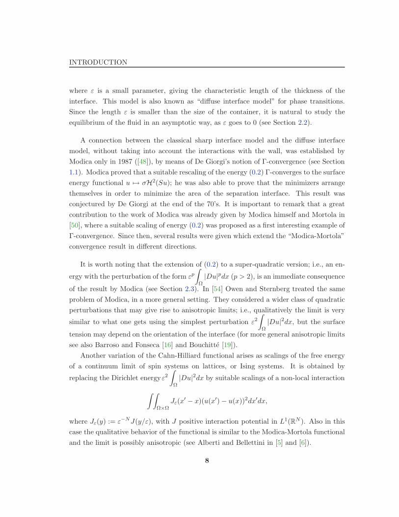
An extension of the classical model for two-phase fluids is obtained by adding to the
energy (0.1) a line tension energy with density τ concentrated along the line Lc ≡ ∂SAW ,
where SAB meets the wall of the container; i.e., along the “contact line” (see Fig. 0.3).
In this model, the capillary energy becomes
E(A) := σH2(SAB) + σAWH2(SAW ) + σBWH2(SBW ) + τH1(Lc). (0.3)
At the end of the 80’s, Modica provided a partial rigorous connection between this clas-
sical model and the diffuse interface model. In [49], Modica added to (0.2) a boundary
contribution of the form λ
∫
∂Ωg(Tu)dH2, where Tu denotes the trace of u on ∂Ω, λ does
not depend on ε, and g is a positive continuous function:
Egε (u) := ε
∫
Ω|Du|2dx+
1
ε
∫
ΩW (u)dx+ λ
∫
∂Ωg(Tu)dHN−1. (0.4)
Confirming a conjecture of Gurtin [43], Modica was able to prove that a sequence of
minimizers (uε) for the energy (0.4) is pre-compact in L1(Ω), each limit point u takes
only the values α and β, and the corresponding phase A := u = α is a solution of the
“liquid-drop” problem1 associated to the energy (0.1).
1The problem of minimizing (0.1) is called “liquid-drop” problem and the existence of a solution isensured by the “wetting condition” σ ≥ |σAW − σBW | (see Section 2.1 and 2.4).
9
INTRODUCTION
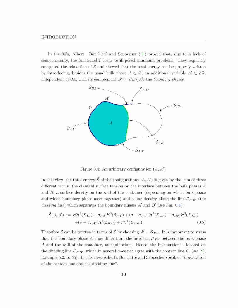
In the 90’s, Alberti, Bouchitte and Seppecher ([9]) proved that, due to a lack of
semicontinuity, the functional E leads to ill-posed minimum problems. They explicitly
computed the relaxation of E and showed that the total energy can be properly written
by introducing, besides the usual bulk phase A ⊂ Ω, an additional variable A′ ⊂ ∂Ω,
independent of ∂A, with its complement B′ := ∂Ω \ A′: the boundary phases.
A
A′
Ω
SBA′
SBB′
SAA′
SAB′
SAB
LA′B′
Figure 0.4: An arbitrary configuration (A,A′).
In this view, the total energy E of the configurations (A,A′) is given by the sum of three
different terms: the classical surface tension on the interface between the bulk phases A
and B, a surface density on the wall of the container (depending on which bulk phase
and which boundary phase meet together) and a line density along the line LA′B′ (the
dividing line) which separates the boundary phases A′ and B′ (see Fig. 0.4):
E(A,A′) := σH2(SAB) + σAWH2(SAA′) + (σ + σAW )H2(SAB′) + σBWH2(SBB′)
+(σ + σBW )H2(SBA′) + τH1(LA′B′). (0.5)
Therefore E can be written in terms of E by choosing A′ = SAW . It is important to stress
that the boundary phase A′ may differ from the interface SAW between the bulk phase
A and the wall of the container, at equilibrium. Hence, the line tension is located on
the dividing line LA′B′ , which in general does not agree with the contact line Lc (see [9],
Example 5.2, p. 35). In this case, Alberti, Bouchitte and Seppecher speak of “dissociation
of the contact line and the dividing line”.
10
INTRODUCTION
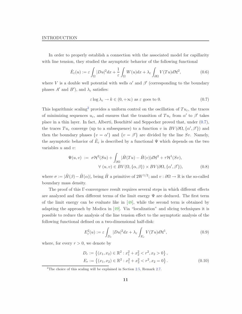
In order to properly establish a connection with the associated model for capillarity
with line tension, they studied the asymptotic behavior of the following functional
Eε(u) := ε
∫
Ω|Du|2dx+
1
ε
∫
ΩW (u)dx+ λε
∫
∂ΩV (Tu)dH2, (0.6)
where V is a double well potential with wells α′ and β′ (corresponding to the boundary
phases A′ and B′), and λε satisfies:
ε log λε → k ∈ (0,+∞) as ε goes to 0. (0.7)
This logarithmic scaling2 provides a uniform control on the oscillation of Tuε, the traces
of minimizing sequences uε, and ensures that the transition of Tuε from α′ to β′ takes
place in a thin layer. In fact, Alberti, Bouchitte and Seppecher proved that, under (0.7),
the traces Tuε converge (up to a subsequence) to a function v in BV (∂Ω, α′, β′) and
then the boundary phases v = α′ and v = β′ are divided by the line Sv. Namely,
the asymptotic behavior of Eε is described by a functional Ψ which depends on the two
variables u and v:
Ψ(u, v) := σH2(Su) +
∫
∂Ω|H(Tu) − H(v)|dH2 + τH1(Sv),
∀ (u, v) ∈ BV (Ω, α, β) ×BV (∂Ω, α′, β′), (0.8)
where σ := |H(β)− H(α)|, being H a primitive of 2W 1/2; and v : ∂Ω → R is the so-called
boundary mass density.
The proof of this Γ-convergence result requires several steps in which different effects
are analyzed and then different terms of the limit energy Ψ are deduced. The first term
of the limit energy can be evaluate like in [48], while the second term is obtained by
adapting the approach by Modica in [49]. Via “localization” and slicing techniques it is
possible to reduce the analysis of the line tension effect to the asymptotic analysis of the
following functional defined on a two-dimensional half-disk:
E2ε (u) := ε
∫
Dr
|Du|2dx+ λε
∫
Er
V (Tu)dH1, (0.9)
where, for every r > 0, we denote by
Dr :=
(x1, x2) ∈ R2 : x2
1 + x22 < r2, x2 > 0
,
Er :=
(x1, x2) ∈ R2 : x2
1 + x22 < r2, x2 = 0
. (0.10)
2The choice of this scaling will be explained in Section 2.5, Remark 2.7.
11
INTRODUCTION
Then the two-dimensional Dirichlet energy (0.9) is replaced on the half-disk Dr by the
H1/2 intrinsic norm on the “diameter” Er. This is possible thanks to the existence of
an optimal constant for the trace inequality involving the L2 norm of the gradient of
a function defined on a two-dimensional domain and the H1/2 norm of its trace on a
line. Hence, the original problem is reduced to the analysis of a new kind of perturbation
problem involving a non-local term:
E1ε (v) := ε
∫∫
I×I
∣
∣
∣
∣
v(t) − v(t′)
t− t′
∣
∣
∣
∣
2
dtdt′ + λε
∫
IV (v) dt, (0.11)
where I is an open interval of R and λε satisfies the condition (0.7).
Alberti, Bouchitte and Seppecher analyze the asymptotic behavior of (0.11) in [8] and
prove that
E1ε
Γ−→ 2k(β′ − α′)2H0(Sv),
and strongly use this result to obtain the boundary term in (0.8).
Note that the qualitative asymptotic behavior of (0.11) departs from all the examples
that we mentioned before. In this case the logarithmic scaling has many special effects.
In contrast with what happens to the classical Modica-Mortola functional (and similar),
in this case all the energy of the limit comes from the non-local term; so that (0.11)
does not produce “equi-partition of energy”. Moreover the limit line tension energy is
not characterized by an optimal profile problem, which instead is the case of the Modica-
Mortola energy and all the variants that we recalled above; so that the transition between
two boundary phases is always optimal as far as it occurs on a layer of order 1/λε.
The same phemonena has been observed in other variants of the energy (0.11), related
to the study of boundary vortices (see Kurzke [46], [47]), or to the study of a phase field
model for defects in crystals (see Garroni and Muller [39]). What those results have in
common is the presence of a non-local singular (non L1) regularization of H1/2 type.
Other results concerning a functional of the type (0.6) are obtained replacing the
Dirichlet energy ε2∫
Ω|Du|2dx by the singular perturbation ε2
∫
Ω|D2u|2dx (see Sousa [55]).
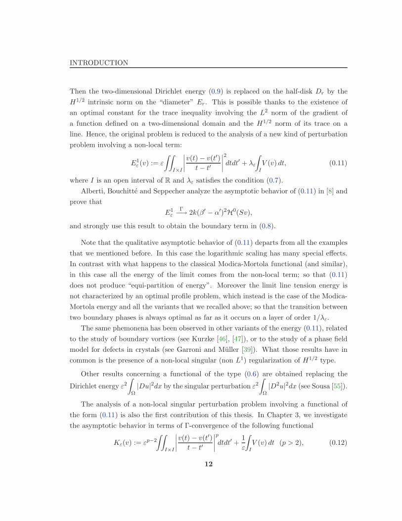
The analysis of a non-local singular perturbation problem involving a functional of
the form (0.11) is also the first contribution of this thesis. In Chapter 3, we investigate
the asymptotic behavior in terms of Γ-convergence of the following functional
Kε(v) := εp−2
∫∫
I×I
∣
∣
∣
∣
v(t) − v(t′)
t− t′
∣
∣
∣
∣
p
dtdt′ +1
ε
∫
IV (v) dt (p > 2), (0.12)
12
INTRODUCTION
as ε→ 0.
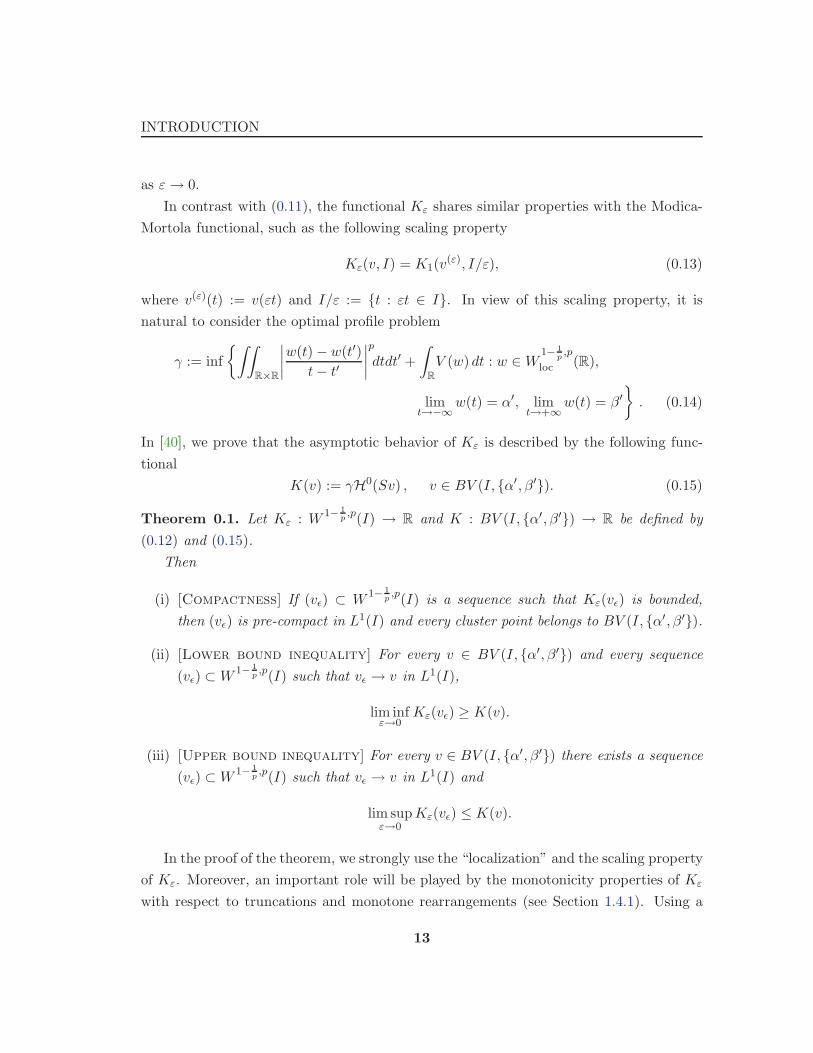
In contrast with (0.11), the functional Kε shares similar properties with the Modica-
Mortola functional, such as the following scaling property
Kε(v, I) = K1(v(ε), I/ε), (0.13)
where v(ε)(t) := v(εt) and I/ε := t : εt ∈ I. In view of this scaling property, it is
natural to consider the optimal profile problem
γ := inf
∫∫
R×R
∣
∣
∣
∣
w(t) − w(t′)
t− t′
∣
∣
∣
∣
p
dtdt′ +
∫
R
V (w) dt : w ∈W1− 1
p,p
loc (R),
limt→−∞
w(t) = α′, limt→+∞
w(t) = β′
. (0.14)
In [40], we prove that the asymptotic behavior of Kε is described by the following func-
tional
K(v) := γH0(Sv) , v ∈ BV (I, α′, β′). (0.15)
Theorem 0.1. Let Kε : W 1− 1p,p(I) → R and K : BV (I, α′, β′) → R be defined by
(0.12) and (0.15).
Then
(i) [Compactness] If (vǫ) ⊂ W1− 1
p,p(I) is a sequence such that Kε(vǫ) is bounded,
then (vǫ) is pre-compact in L1(I) and every cluster point belongs to BV (I, α′, β′).
(ii) [Lower bound inequality] For every v ∈ BV (I, α′, β′) and every sequence
(vǫ) ⊂W1− 1
p,p(I) such that vǫ → v in L1(I),
lim infε→0
Kε(vǫ) ≥ K(v).
(iii) [Upper bound inequality] For every v ∈ BV (I, α′, β′) there exists a sequence
(vǫ) ⊂W 1− 1p,p(I) such that vǫ → v in L1(I) and
lim supε→0
Kε(vǫ) ≤ K(v).
In the proof of the theorem, we strongly use the “localization” and the scaling property
of Kε. Moreover, an important role will be played by the monotonicity properties of Kε
with respect to truncations and monotone rearrangements (see Section 1.4.1). Using a
13
INTRODUCTION
monotone rearrangement result we will also prove that the infimum in (0.14) is not trivial
and is achieved.
The study of the functional Kε has its own interest, showing that the analysis per-
formed by Modica and Mortola is stable under a much larger class of perturbations,
including non-local singular perturbations, as far as they are not “critical” in the sense of
trace imbedding. On the other hand it has also been the first step towards the compre-
hension of the main problem of this thesis, that concerns the study of a functional similar
to (0.6), but with a super-quadratic growth in the perturbation term.
For every ε > 0, we consider the functional Fε defined by
Fε(u) := εp−2
∫
Ω|Du|pdx+
1
εp−2p−1
∫
ΩW (u)dx+
1
ε
∫
∂ΩV (Tu)dH2. (0.16)
This functional still describes a capillarity problem (0.5), but its asymptotic behavior
brings out different characteristics with respect to the energy (0.6).
Let us briefly analyze the asymptotic behavior of the functional Fε. If (uε) is a
sequence with equi-bounded energy, we observe that the term1
εp−2p−1
∫
ΩW (uε)dx forces uε
to take values close to α and β, while the term εp−2
∫
Ω|Duε|pdx penalizes the oscillations of
uε. We will see that when ε tends to 0, the sequence (uε) converges (up to a subsequence)
to a function u, that belongs to BV (Ω), which takes only the values α and β. Moreover
each uε has a transition from the value α to the value β in a thin layer close to the surface
Su, which separates the bulk phases u = α and u = β. Similarly, the boundary term
of Fε forces the traces Tuε to take values close to α′ and β′, and the oscillations of the
traces Tuε are again penalized by the integral εp−2
∫
Ω|Duε|pdx. Then, as for the case of
the functional studied by Alberti, Bouchitte and Seppecher, we expect that the sequence
(Tuε) converges to a function v in BV (∂Ω) which takes only the values α′ and β′, and
that a concentration of energy occurs along the line Sv, which separates the boundary
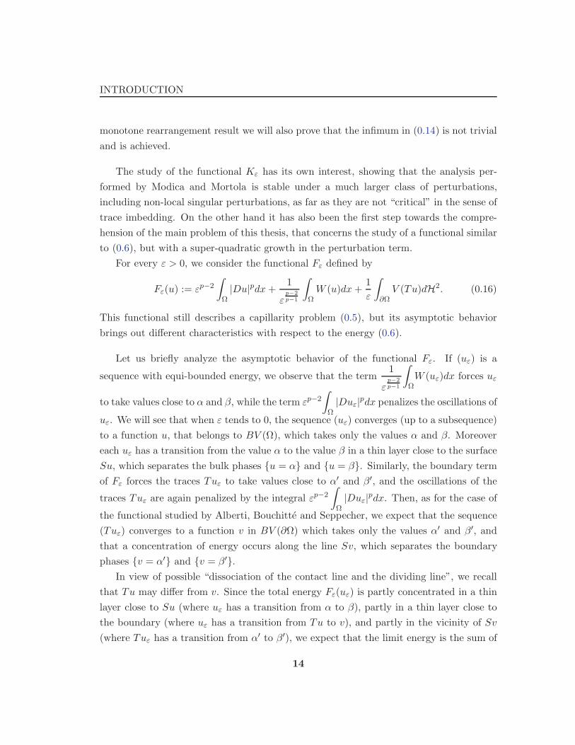
phases v = α′ and v = β′.In view of possible “dissociation of the contact line and the dividing line”, we recall
that Tu may differ from v. Since the total energy Fε(uε) is partly concentrated in a thin
layer close to Su (where uε has a transition from α to β), partly in a thin layer close to
the boundary (where uε has a transition from Tu to v), and partly in the vicinity of Sv
(where Tuε has a transition from α′ to β′), we expect that the limit energy is the sum of
14
INTRODUCTION
a surface energy concentrated on Su, a boundary energy on ∂Ω (with density depending
on the gap between Tu and v), and a line energy concentrated along Sv.
The asymptotic behavior of the functional Fε is described by a functional Φ which
depends on the two variables u and v. If W is a primitive of W (p−1)/p, we prove that for
every (u, v) ∈ BV (Ω, α, β) ×BV (∂Ω, α′, β′)
Φ(u, v) = σpH2(Su) + cp
∫
∂Ω|W(Tu) −W(v)|dH2 + γpH1(Sv), (0.17)
where Su and Sv denote the jump set of u and v, respectively; cp and σp are two positive
constants defined by cp :=p
(p− 1)p/(p−1); σp := cp|W(β) − W(α)|; γp is given by the
optimal profile problem
γp := inf
∫
R2+
|Du|pdx+
∫
R
V (Tu)dH1 : u ∈ L1loc(R
2+) :
∫
R2+
|Du|pdx is finite,
limt→−∞
Tu(t)=α′, limt→+∞
Tu(t)=β′
.(0.18)
In Chapter 6 we prove the main convergence result, stated in the following theorem.
Theorem 0.2. Let Fε : W 1,p(Ω) → R and Φ : BV (Ω, α, β) × BV (∂Ω, α′, β′) → R
defined by (0.16) and (0.17).
Then
(i) [Compactness] If (uε) ⊂ W 1,p(Ω) is a sequence such that Fε(uε) is bounded,
then (uε, Tuε) is pre-compact in L1(Ω) × L1(∂Ω) and every cluster point belongs
to BV (Ω, α, β) ×BV (∂Ω, α′, β′).
(ii) [Lower Bound Inequality] For every (u, v) ∈ BV (Ω, α, β)×BV (∂Ω, α′, β′)and every sequence (uε) ⊂ W 1,p(Ω) such that uε → u in L1(Ω) and Tuε → v in
L1(∂Ω),
lim infε→0
Fε(uε) ≥ Φ(u, v).
(iii) [Upper Bound Inequality] For every (u, v) ∈ BV (Ω, α, β)×BV (∂Ω, α′, β′)there exists a sequence (uε) ⊂ W 1,p(Ω) such that uε → u in L1(Ω), Tuε → v in
L1(∂Ω) and
lim supε→0
Fε(uε) ≤ Φ(u, v).
15
INTRODUCTION
Notice that the limit functional Φ is of the same form of the functional Ψ defined by
(0.8); that is, the Γ-limit of Eε. Nonetheless, the variation in the power of the gradient
in the perturbation term is not a simple generalization of the quadratic case, since the
structure of these two problems is different. In fact, in the quadratic case the natural
scaling of the energy is logarithmic and this implies that the profile in which the phase
transition occurs on the boundary is not important for the first order of the energy. While,
the super-quadratic case is characterized by an optimal profile problem which determines
the line tension in the limit. This characteristic will be a double-edged sword in the proof
of Theorem 0.2: some arguments will be simplified by the presence of an optimal profile
problem, some other will require more care.
The proof of Theorem 0.2 requires several steps. We can deduce the terms of the limit
energy Φ, localizing three effects: the bulk effect, the wall effect and the boundary effect.
In the bulk term, the limit energy can be evaluate like in [48]. We will use the super-
quadratic version of the Modica-Mortola functional (see Section 2.2).
The second term of Φ can be obtained by adapting the approach by Modica in [49].
Since the results by Modica concerns a functional with quadratic growth in the singular
perturbation term and with a boundary contribution of the form λ
∫
∂Ωg(Tu)dH2, with
λ not depending on ε and g a positive continuous function, we need to adapt part of the
results in [49] to our goal (see Chapter 4).
Finally, the boundary effect requires a deeper analysis. The main strategy consists in:
first reducing to the case in which the boundary is “flat”; hence studying the behavior of
the original energy in the three-dimensional half ball; then reducing the problem of one
dimension via a slicing argument. Thus, the main problem becomes the analysis of the
asymptotic behavior of the following two-dimensional functional
Hε(u) := εp−2
∫
D1
|Du|pdx+1
ε
∫
E1
V (Tu)dH1, (0.19)
where D1 and E1 are defined by (0.10). Chapter 5 is devoted to the analysis of the
asymptotic behavior of (0.19) and to the proof of the existence of a minimum for the
optimal profile (0.18). We remark that we can not reduce further to a one dimensional
problem, like in the case p = 2, where one can use the optimal trace imbedding. In spite
of that, as a consequence of equi-partition of the energy, the optimal profile problem plays
an important role in the proof. In this respect, the case p = 2 represent the critical case
in the context of this type of non-local perturbations.
16
INTRODUCTION
A similar dichotomy occurs in the case of Ginzburg-Landau problems (see for instance
Alberti, Baldo and Orlandi [4] versus Desenzani and Fragala [29]).
Plan of the thesis
Chapter 1. We introduce the notion of Γ-convergence, with its main properties, and we state
some preliminary results about Young measures, the slicing method and monotone
rearrangements.
Chapter 2. We briefly explain the Cahn-Hilliard model for phase transitions and state some pre-
liminary convergence results for Cahn-Hilliard functionals, with or without taking
into account the interactions with the wall.
Chapter 3. We study the asymptotic behavior of the non-local perturbed energy (0.12), pro-
viding a complete proof of the Γ-convergence result stated in Theorem 0.1 and a
characterization of the optimal profile problem (0.14).
Chapter 4. We introduce the main problem of this thesis, namely the analysis of the asymp-
totic behavior of the functional (0.16); we also exhibit the strategy of the proof of
Theorem 0.2.
Chapter 5. We study the asymptotic behavior of the two-dimensional functional (0.19) and we
provide a proof of the existence of a minimum for the optimal profile problem (0.18).
Chapter 6. We prove the main results in this thesis, namely the compactness and the Γ-
convergence results stated in Theorem 0.2.
17
Chapter 1
Preliminaries
In this chapter, we briefly give a definition of Γ-convergence and we state some results
about Young measures, the slicing method and the behavior of certain classes of integral
functionals with respect to the monotone rearrangement of functions. Every statement
in this chapter will be presented in the form that better fits to our purposes.
Notation
In this work, we consider different domains A with dimensions N = 1, 2, 3; more
precisely, A will always be a bounded open set either of RN . We denote by ∂A the
boundary of A relative to the ambient manifold; ∂A is always assumed to be Lipschitz
regular. Unless otherwise stated, A is endowed with the corresponding N -dimensional
Hausdorff measure, HN (see [32], Chapter 2). We write
∫
Afdx instead of
∫
AfdHN , and
|A| instead of HN .
TheN -dimensional density of A at x is the limit (if it exists) of HN (A ∩Br(x))/ωNrN ,
where Br(x) is the ball centered in x with radius r and ωN is the measure of the unit ball
in RN .
The essential boundary of A is the set of all points where A has neither density 0 nor
1 and where the density does not exist. Since the essential boundary agrees with the
topological boundary when the latter is Lipschitz regular, we also denote the essential
boundary by ∂A.
For every u ∈ L1loc(A), we denote by Su the complement of the set of Lebesgue points
of u; i.e., the jump set, the set where the upper and lower approximate limits of u differ or
18
CHAPTER 1. Preliminaries
are not finite. We denote by Du the derivative of u in the sense of distributions. As usual,
for every p ≥ 1, W 1,p(A) is the Sobolev space of all u ∈ Lp(A) such that Du ∈ Lp(A);
BV (A) is the space of all u ∈ L1(A) with bounded variation; i.e., such that Du is a
bounded Borel measure on A.
For every s ∈ (0, 1) and every p ≥ 1, W s,p is the space of all u ∈ Lp(A) such that the
fractional semi-norm
∫ ∫
A×A
|u(x) − u(x′)|p|x− x′|sp/N dxdx′ is finite.
We denote by T the trace operator which maps W 1,p(A) onto W 1−1/p,p(∂A) and
BV (A) onto L1(∂A). For details and results about the theory of BV functions and
Sobolev spaces we refer to [32] and [1].
Throughout this thesis, all the functions and sets are assumed to be Borel measurable.
Moreover, we always use the term “sequence” also to denote families (of functions) labelled
by continuous parameter ε, which tends to 0. Thus, a subsequence of (uε) is any sequence
(uεk) such that εk → 0 as k → +∞, and we say that (uε) is pre-compact if every
subsequence admits a convergent sub-subsequence. To simplify the notation, we often do
not relabel subsequences.
1.1 Γ-Convergence
Γ-convergence was introduced by De Giorgi in the early 70’s. Its first definition was
stated in [28], where all the main properties were presented. Γ-convergence is linked to
previous notions of convergence such as Mosco’s convergence (see [51]) or Kuratowski’s
convergence of sets. Indeed, Γ-convergence of a sequence of functions can be viewed as a
convergence of their epigraphs (epiconvergence), just like semicontinuity can be seen as a
property of the epigraphs.
We give the definition and the main properties of Γ-convergence as a notion of con-
vergence for functions on a generic metric space X. Therefore, in the following, u is an
element of X and F a function from X to R := [−∞,+∞]. Here, we present a simplified
version of the original definition; we refer to [2] (see [27] and [23] for a detailed treatment
of the general theory of Γ-convergence and various applications).
Definition 1.1. We say that a sequence Fε : X → R Γ-converges to F on X as ε to 0 if
for every u ∈ X the following conditions hold:
19
CHAPTER 1. Preliminaries
(i) [Lower bound inequality] for every sequence (uε) converging to u in X
F (u) ≤ lim infε→0
Fε(uε); (1.1)
(ii) [Upper bound inequality] there exists a sequence (uε) converging to u in X such
that
F (u) = lim supε→0
Fε(uε). (1.2)
Condition (i) means that whatever sequence we choose to approximate u, the value of
Fε(uε) is, in the limit, larger than F (u). On the other hand, condition (ii) implies that
this bound is sharp; that is, there always exists a sequence (uε) which approximates u so
that Fε(uε) → F (u).
When proving a Γ-convergence result, it is convenient to reduce the amount of verifi-
cations and constructions. To this aim, note that if (i) holds, then equality (1.2) can be
replaced by
F (u) ≥ lim supε→0
Fε(uε).
From Definition 1.1, we may deduce the following properties of Γ-convergence:
(p1) The Γ-limit F is always lower semicontinuous on X;
(p2) Γ-limits are stable under continuous perturbations. This means that one Γ-limit is
computed we do not have to redo all computations if “lower-order terms” are added.
Conversely, we can always remove such terms to simplify calculations;
(p3) Under suitable conditions Γ-convergence implies convergence of minimum values
and minimizers. Note that some minimizers of the Γ-limit may not be limit of
minimizers, so that Γ-convergence may be interpreted as a choice criterion.
Now, we pass to describe how this notion of variational convergence will be used.
Assume that for every ε > 0 we are given a function uε which minimizes the functional
Fε on X, and that we want to know what happens to uε as ε goes to 0. Sometimes, the
minimizers uε can be written via some explicit formula from which we can deduce all
information about its asymptotic behavior. In many instances, no such representation of
uε is available and then we can exploit the fact that each uε solves the Euler-Lagrange
equation associated with Fε and try to understand which kind of limit equation is verified
by a limit point u of (uε). Another possibility is to use the notion of Γ-convergence.
20
CHAPTER 1. Preliminaries
Suppose that we have computed the Γ-limit F of the functional Fε, by property (p3)
we can conclude that any limit point u is a minimizer of F , and in particular solves the
Euler-Lagrange equation associated with F .
Notice that such a strategy makes sense only if we know a priori that the minimizing
sequence (uε) is pre-compact in X. A Γ-convergence result for the functional Fε should
always be paired with a “compactness result” for the corresponding minimizing sequences
(uε). According to this viewpoint, the Definition 1.1 have to be completed by the following
equi-coercivity of Fε:
(iii) [Compactness] If (uε) is a sequence such that Fε(uε) is bounded, then (uε) is pre-
compact in X.
1.1.1 Choice of interesting rescalings
If uε minimizes Fε, then it also minimizes λεFε, for every positive λε. Hence, we can
recover information about the limit points of (uε) also by the Γ-limit of λεFε. Notice
that different choices of the scaling factor λε generate different Γ-limits, which provide
different information. For instance, it may happen that the functional Fε converges to a
constant functional F , and consequently we have no information about the limit points
u, while the Γ-limit of functionals λεFε may be less trivial. Therefore, before trying to
verify Definition 1.1 and a compactness result, it is important to find a suitable λε so
that the Γ-limit of the rescaled functional λεFε gives the largest amount of information.
Sometimes this optimal rescaling is evident but sometimes it is not.
1.2 Young Measures
Young measures (also called “generalized functions”) were introduced by Young in
the 30’s to solve optimal control problems that have no classical solution. The idea is to
replace functions which take values in a set A ⊂ RN by functions that take values in the
space of probability measures. For instance, a mixture of two states can be represented
by a convex combination of two Dirac measures (see [58]). Since then, Young measures
arguments have been used in various problems.
In the following, we introduce Young measures associated to a sequence, that are
appropriate to describe the limit oscillation behavior of the sequence self. In few words,
21
CHAPTER 1. Preliminaries
under mild assumption, any sequence (un) of functions has a subsequence which converges
to some Young measure.
We state some results, which will be useful to our purposes. We refer to Muller in [53]
and Valadier in [56].
1.2.1 The fundamental theorem on Young measures and applications
By C0(RN ) we denote the closure of continuous functions on R
N with compact support.
The dual of C0(RN ) can be identified with the space M(RN ) of signed Radon measures
with finite mass via the pairing
〈µ, f〉 =
∫
R
fdµ.
A map µ : A→ M(RN ) is called “weak-∗ measurable” if the functions x→ 〈µ(x), f〉 are
measurable for all f ∈ C0(RN ).
Theorem 1.2. ([53], Theorem 3.1, p. 31). Let A ⊂ RN be a measurable set of finite
measure and let un : A→ RN be a sequence of measurable functions. Then there exists a
subsequence (unk) and a weak-∗ measurable map ν : A→ M(RN ) such that the following
statements hold:
(i) νx ≡ ν(x) ≥ 0, ‖νx‖M(RN ) =
∫
RN
dνx ≤ 1, for a.e. x ∈ A.
(ii) For all f ∈ C0(RN )
f(unk)
∗ f in L∞(A),
where
f = 〈νx, f〉 =
∫
RN
fdνx.
(iii) Let K ⊂ RN be compact. Then
supp(νx) ⊂ K for a.e.x ∈ A if dist(unk,K) → 0 in measure.
(iv) Furthermore, one has
(i’)‖νx‖M(R) = 1 for a.e. x ∈ A
if and only if
limM→+∞
supk
||unk| ≥M| = 0.
22
CHAPTER 1. Preliminaries
(v) If (i’) holds, if B ⊂ A is measurable, if f ∈ C(RN) and if f(unk) is relatively weakly
compact in L1(B), then
f(unk) f in L1(B), f(x) = 〈νx, f〉.
(vi) If (i’) holds, then in (iii) one can replace “if” by “if and only if”.
Definition 1.3. The map ν : E → M(RN ) is called the Young measure associated to (or
generated by) the sequence (unk).
Note that every weak-∗ measurable map ν : E → M(RN ) that satisfies (i) of Theorem
1.2 is generated by some sequence (un).
Example.
Let us show a typical application of Theorem 1.2.
If (un) is bounded in Lp(A) and the continuous function f has a certain growth to +∞,
like |f(t)| ≤ C(1 + |t|q), with q < p.
Then, by (v), it follows
f(unk) f in Lp/q(A).
In particular, for p > 1, choosing f ≡ id, we have
unk u with u(x) = 〈νx, id〉, ∀x ∈ A.
The measure νx describes the probability of finding a certain value in the sequence
(unk) in a small neighborhood Br(x) in the limits k → ∞ and r → 0.
Corollary 1.4. ([53], Corollary 3.2, p. 34). Let (un) be a sequence of measurable func-
tions from A to RN that generates the Young measures ν : A→ M(RN ). Then
un → u in measure if and only if νx = δu(x) a.e. in A.
Another property of the Young measures associated to a sequence is stated in the
following theorem, which we will use to recover important compactness results. We denote
by Y(A) the family of all weakly-∗ measurable maps ν : A → P(R), where P(R) is the
set of probability measures on R.
23
CHAPTER 1. Preliminaries
Theorem 1.5. ([56], Theorem 16, p. 166). Let un be a bounded sequence in L1(A).
There exists a subsequence unkand a map ν ∈ Y(A) such that, for every Caratheodory
function f : R → [0,+∞) we have
lim infk→+∞
∫
Af(x, unk
(x))dx ≥∫
Afdx, (1.3)
where f(x) :=
∫
R
f(x, t)dνx(t).
1.3 The slicing method
In this section, we describe a well-known method often used to recover compactness
and lower bound inequalities through the study of problems of lower dimension via a
slicing argument. The slicing method has been introduced by Ambrosio to treat free-
discontinuity problems (see [10]) and has been used to prove various results also within
the theory of phase transitions (see [5] and [9]).
Let us try to understand how the slicing method will be used by looking at the
Modica-Mortola functional
Eε(u) := ε
∫
A|Du|2dx+
1
ε
∫
AW (u)dx,
defined on H1(A), with A bounded open set of RN . We may examine the behavior of Eε
on one-dimensional sections as follows:
for each e unit vector in RN we consider the hyperplane
Πe :=
z ∈ RN : 〈z, e〉 = 0
passing through 0 and orthogonal to e. We denote by Ae the projection of A onto Πe;
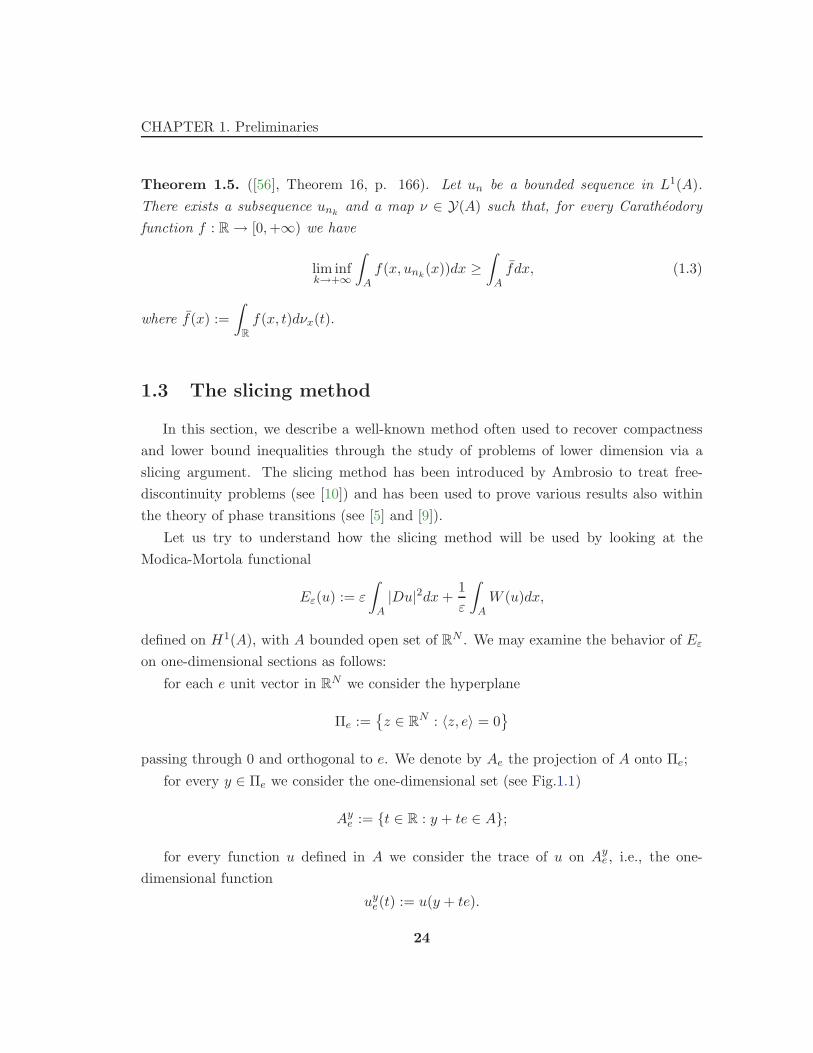
for every y ∈ Πe we consider the one-dimensional set (see Fig.1.1)
Aye := t ∈ R : y + te ∈ A;
for every function u defined in A we consider the trace of u on Aye , i.e., the one-
dimensional function
uye(t) := u(y + te).
24

CHAPTER 1. Preliminaries
e A
Πe
y
Aye
Figure 1.1: A section of the domain A.
Now, we are ready to obtain a lower bound for the Γ-liminf of Eε by looking at the
limit of the functionals induced by Eε on the one-dimensional sections. Thanks to Fubini’s
Theorem, we rewrite Eε as
Eε(u) =
∫
Πe
∫
Aye
(
ε|Du(y + te)|2 +1
εW (u(y + te))
)
dtdy. (1.4)
The main idea of the slicing method is using the Γ-limit of the one-dimensional functionals
v 7→∫
Aye
(
ε|v′(t)|2 +1
εW (v(t))
)
dt
and the inequality from (1.4)
Eε(u) ≥∫
Πe
∫
Aye
(
ε|(uye)′(t)|2 +1
εW (uye(t))
)
dtdy,
to obtain a lowerbound for the Γ-liminf of Eε, by Fatou’s Lemma and optimizing the
choice of e.
In the following subsections, we recall some general results regarding the slicing of
Sobolev functions.
25
CHAPTER 1. Preliminaries
1.3.1 Some slicing results
For the sake of simplicity, we work only with one-dimensional slicing, but the following
results are true for slicing with arbitrary dimension. Let A, e, Ae and Aye be given as
before and take a Borel function u in A. By Fubini’s Theorem u belongs to Lp, 1 ≤ p <∞,
if and only if uye belongs to Lp(Aye) for a.e. y ∈ Ae and the function y → ‖uye‖Lp belongs to
Lp(Ae). Similarly, given a sequence (uk) ⊂ Lp(A) which converges to u in Lp(A), we have
that (up to a subsequence) (uk)ye converges to uye in Lp(Aye) for a.e. y ∈ Aye . Moreover, if
(uk)ye converges to uye for a.e. y ∈ Ae and the functions |uk|p are equi-integrable, then uk
converges to u in Lp(A).
Proposition 1.6. ([32], Theorem 2, p. 164). Let u ∈ Lp(A) be given. If e is an arbitrary
unit vector and u belongs to W 1,p(A), then uye ∈ W 1,p(Aye) for a.e. y ∈ Ae, and the
derivative (uye)′(t) agrees with the partial derivative ∂eu(y + te) for a.e. y ∈ Ae and
t ∈ Aye . Conversely, u belongs to W 1,p(A) if there exist N linearly independent unit
vectors e such that uye ∈W 1,p(Aye) for a.e. y ∈ Ae and the function y → ‖(uye)′‖Lp belongs
to Lp(Ae).
Proposition 1.7. ([32], Section 5.10, p. 216). Let a Borel set E ⊂ A be given. If E has
finite perimeter in A, then Eye has finite perimeter in Aye and ∂(Eye ∩ Aye) = (∂E ∩ A)ye
for a.e. y ∈ Ae, and∫
Ae
H0(∂Eye ∩Aye)dy =
∫
∂E∩A〈vE , e〉. (1.5)
Conversely, E has finite perimeter in A if there exist N linearly independent unit vectors
e such that the integral of H0(∂Eye ∩Aye) over all y ∈ Ae is finite.
We establish a connection between the compactness of a family of functions in L1(RN )
and the compactness of the traces of these functions. We need to recall the definition of
δ-dense family of functions.
Definition 1.8. Let F and F ′ be two families of functions on A. For every δ > 0, we
say that the family F ′ is δ-dense in F if F lies in a δ-neighborhood of F ′ with respect to
the L1(A) topology.
According to previous notation, for every family F of functions on A, we denote by
Fye := (uye)u∈F the family of functions on Aye .
26
CHAPTER 1. Preliminaries
Theorem 1.9. ([9], Theorem 6.6, pag. 42). Let F be a family of functions v : A →[−m,m] and assume that there exist N linearly independent unit vectors e which satisfy
the following property:
For every δ > 0 there exists a family Fδ δ-dense in F such that
(Fδ)ye is pre-compact in L1(A) for HN−1-a.e. y ∈ Ae. (1.6)
Then F is pre-compact in L1(A).
We will use the L1-pre-compactness criterion by slicing of Theorem 1.9 to prove the
pre-compactness of the traces of the minimizing sequence of the functional Fε, defined by
(0.16).
1.3.2 Isometry defect
When we work with slicings, we may also want to evaluate “the error we make” when
we perturb a three-dimensional domain to get a two-dimensional one. To this aim, we
define the “isometry defect”, introduced by Alberti, Bouchitte and Seppecher in [9].
As usual, we denote by O(3) the set of linear isometries on R3.
Definition 1.10. Let A1, A2 ⊂ R3 and let Ψ : A1 → A2 bi-Lipschitz homeomorphism.
Then the “isometry defect δ(Ψ) of Ψ” is the smallest constant δ such that
dist(DΨ(x), O(3)) ≤ δ, for a.e. x ∈ A1. (1.7)
HereDΨ(x) is regarded as a linear mapping of R3 into R
3. The distance between linear
mappings is induced by the norm ‖ · ‖, which, for every L, is defined as the supremum of
|Lv| over all v such that |v| ≤ 1. Hence, for every L1, L2 : R3 → R
3:
dist(L1, L2) := supx:|x|≤1
|L1(x) − L2(x)|.
Given L1, L2 : A1 → A2, with L1 isometry, such that there exists δ < 1 such that
‖L1 − L2‖ ≤ δ.
Then, L2 is invertible and ‖L−11 − L−1
2 ‖ ≤ δ/(1 − δ).
By (1.7), it follows
dist(DΨ−1(y), O(3)) ≤ δ/(1 − δ), for a.e. y ∈ A2,
27
CHAPTER 1. Preliminaries
and then
δ(Ψ−1(y)) ≤ δ(Ψ(y))/(1 − δ(Ψ(y))), for a.e. y ∈ A2.
Inequality (1.7) also implies that
‖DΨ(x)‖ ≤ 1 + δ(Ψ) for a.e. x ∈ A1,
and then Ψ is (1 + δ(Ψ))-Lipschitz continuous on every convex subset of A1. Similarly,
Ψ−1 is (1 − δ(Ψ))−1-Lipschitz continuous on every convex subset of A2.
For every A ⊂ R3 and every A′ ⊂ ∂A, let Fε : W 1,p(A) → R be the functional defined
by (0.16); that is:
Fε(u,A,A′) := εp−2
∫
A|Du|pdx+
1
εp−2p−1
∫
AW (u)dx+
1
ε
∫
A′
V (Tu)dH2.
The following proposition holds.
Proposition 1.11. Let A1, A2 ⊂ R3,Ψ : A1 → A2 a bi-Lipschitz homeomorphism, A′
1 ⊂∂A1, A
′2 ⊂ ∂A2, be given such that Ψ(A′
1) = A′2 and δ(Ψ) < 1. Then for every u ∈
W 1,p(A2)
Fε(u,A2, A′2) ≥ (1 − δ(Ψ))p+3Fε(u Ψ, A1, A
′1).
Proof. The proof is a simple modification of the one by Alberti Bouchitte and Seppecher
in [9] (Proposition 4.9, p. 25), where they treat the case p = 2.
By (1.10), we get ‖DΨ(x)‖ ≤ 1 + δ(Ψ) for x a.e. in A1, that implies
|D(u Ψ)(x)| ≤ (1 + δ(Ψ))|((Du) Ψ)(x)|, a.e. in A1. (1.8)
Let g1 and g2 denote the inverse of Ψ and the restriction to ∂A2 of the inverse of Ψ,
respectively:
g1(x) := (Ψ)−1(x), g2(x) := (Ψ|∂A2)−1(x).
g1 and g2 are locally Lipschitz and such that
|Jg1| ≤ (1 − δ(Ψ))3 a.e. on A2 and |Jg2| ≤ (1 − δ(Ψ))3 a.e. on ∂A2. (1.9)
Since δ(Ψ) < 1 then
(1 + δ(Ψ)) ≤ (1 − δ(Ψ))−1. (1.10)
Thus, using the estimates on the Jacobian determinants (1.9) and the inequality (1.10),
we obtain the desired conclusion by changing-variable formula. 2
28

CHAPTER 1. Preliminaries
Proposition 1.12. ([9], Proposition 4.10, p. 25). For every x ∈ ∂Ω and every positive
r smaller than a certain critical value rx > 0, there exists a bi-Lipschitz map Ψr : Dr →Ω ∩Br(x) such that
(a) Ψr takes Dr onto Ω ∩Br(x) and Er onto ∂Ω ∩Br(x);
(b) Ψr is of class C1 on Dr and ‖DΨr − I‖ ≤ δr everywhere in Dr, where δr → 0 as
r → 0.
Note that, in particular, the isometry defect of Ψr vanishes as r → 0.
Figure 1.2: Construction of Ψ := Ψ−11 Ψ2 Ψ1 ([9], Fig. 5, p. 26).
1.4 Rearrangement results
In this section we state some rearrangement results that we will use in the sequel.
Rearrangement problems have been widely studied in the literature (see for instance
[45], [15], [14], [3] and [17]). Our main concern is the behavior with respect to the
rearrangement of certain classes of integral functionals.
Before starting definitions and results, we stress that we use the terms increasing
and decreasing in the weak sense, that is, to mean non-decreasing and non-increasing
respectively.
1.4.1 Monotone rearrangement in one-dimension
We refer to [5] and [38].
29
CHAPTER 1. Preliminaries
We denote by I the open bounded interval (a, b) in R.
Definition 1.13. For every measurable function v : I → R we define the monotone
increasing rearrangement of v as the function v∗ : I → R by
v∗(t+ a) := sup λ : | s ∈ (a, b) : v(s) ≤ λ | ≤ t , ∀t ∈ (0, b− a).
The following theorems hold.
Theorem 1.14. [[5], Theorem 5.6, p. 557]. Let W be a non-negative continuous function
on [α′, β′] such that W (α′) = W (β′) = 0. For every v : I → R, the following equality
holds:∫
IW (v)dx =
∫
IW (v∗)dx, (1.11)
where v∗ is the increasing rearrangement of v.
Theorem 1.15. [[38], Theorem I.1, p. 67]. Let J, P : R → R be two continuous even
functions such that
(i) J(es) is convex in R and J(|s|) → +∞ as |s| → +∞;
(ii) P (|s|) → 0 as |s| → +∞.
Then, for every measurable function v : I → R such that
∫ ∫
I×IJ
(
v(t′) − v(t)
P (t′ − t)
)
dt′dt is
finite, the following inequality holds:∫ ∫
I×IJ
(
v∗(t′) − v∗(t)
P (t′ − t)
)
dt′dt ≤∫ ∫
I×IJ
(
v(t′) − v(t)
P (t′ − t)
)
dt′dt,
where v∗ is the monotone increasing rearrangement of v in I.
As an immediate consequence of Theorem 1.15, we have that replacing a function
v by its increasing rearrangement decreases the p-power of the fractional semi-norm of
W 1−1/p,p(I):∫ ∫
I×I
|v∗(t′) − v∗(t)|p|t′ − t|p dt′dt ≤
∫ ∫
I×I
|v(t′) − v(t)|p|t′ − t|p dt′dt. (1.12)
Hence, by (1.11) and (1.12) with J(·) = | · |p and P (·) = | · |, we obtain that the same
monotonicity property with respect to monotone increasing rearrangements holds for the
following non-local functional:
Kε(v) := εp−2
∫∫
I×I
∣
∣
∣
∣
v(t) − v(t′)
t− t′
∣
∣
∣
∣
p
dtdt′ +1
ε
∫
IV (v) dt.
30
CHAPTER 1. Preliminaries
1.4.2 Monotone rearrangement in one direction
We state a rearrangement result for the energy of Sobolev functions defined on bounded
cylinders; we refer to Kawohl [45] and Berestycky and Lachand-Robert [17].
Let ω be a smooth bounded domain in RN−1 and let I be a bounded open interval of
R, we denote by Q := I × ω the bounded cylinder in RN . For every measurable function
u : Q → R, we denote by u⋆ the monotone rearrangement in direction x1 of u; i.e., the
function u⋆ : Q → R which is increasing in I with respect to x1 (for almost all x′ ∈ ω),
and such that for every λ ∈ R and for every x′ ∈ ω :
|
x1 ∈ I : u(x1, x′) ≥ λ
| = |
x1 ∈ I : u⋆(x1, x′) ≥ λ
|.
Theorem 1.16. [[45], Corollary 2.14 , p. 51, and [17], Theorem 3, p. 10]. If u belongs
to W 1,p(Q), then its monotone increasing rearrangement in direction x1 u⋆ belongs to
W 1,p(Q) and∫
Q|Du⋆|pdx ≤
∫
Q|Du|pdx.
This result will be a key point in the proof of the existence of a minimum for the
optimal profile problem (0.14).
31
Chapter 2
Phase transitions and known
results
A phase transition is a change of a thermodynamic system from one phase to another.
The main characteristic of a phase transition is a sudden transformation in one or more
physical properties, like heat capacity, with a change in a thermodynamic variable such
as the temperature. We can find many phase transition events, like the transitions be-
tween the solid, liquid and gaseous phases, due to effect of temperature and pressure, the
transitions between the ferromagnetic and paramagnetic phases of magnetic materials at
the Curie point, the emergence of superconductivity in certain metals when cooled below
a critical temperature, and so.
In the following, we pay attention to the classical model for two-phase fluids and its
mathematical approach initiated by Gibbs and revisited by Cahn and Hilliard.
2.1 The classical model for phase transitions
In the classical theory of phase transitions, a two-phase systems is modeled as follows:
the container is represented by a bounded regular domain Ω in R3; every configuration
of the fluid is described by a mass density u on Ω which takes only two values, α and β,
corresponding to the phases A := u = α and B := u = β = Ω \ A. The singular set
of u (the set of discontinuity points of u) is the interface between the two phases, that we
denote by Su.
The space of admissible configurations is given by all u : Ω → α, β under some
volume constraint. The energy is located on the interface SAB := Su which separates the
32

CHAPTER 2. Phase transitions and known results
Ω
SAB
SBW
SAW
AB
Figure 2.1: The classical model for phase transitions.
two phases and on the contact surfaces SAW := ∂A ∩ ∂Ω and SBW := ∂B ∩ ∂Ω between
the wall of the container and the phases A and B (see Fig. 2.1).
The equilibrium configurations are assumed to minimize the capillary energy
E0(A) := σH2(SAB) + σAWH2(SAW ) + σBWH2(SBW ), (2.1)
where the positive constants σ, σAW and σBW are referred to as surface tension. The
problem of minimizing (2.1) is called liquid-drop problem and the existence of a solution
is assured by the wetting condition:
σ ≥ |σAW − σBW |.
At the equilibrium, the interface SAB has constant mean curvature and meets the wall of
the container with a constant contact angle ϑ, which satisfies the Young’s law
ϑ = arccosσAW − σBW
σ.
See, for instance Finn in [33].
2.2 The Cahn-Hilliard model for phase transitions
In the late 50’s, Cahn and Hilliard [24] proposed an alternative way to study two-phase
fluids. They followed the continuum mechanics approach by Gibbs and assumed that
33
CHAPTER 2. Phase transitions and known results
the transition is not given by a separating interface, but is a continuous phenomenon
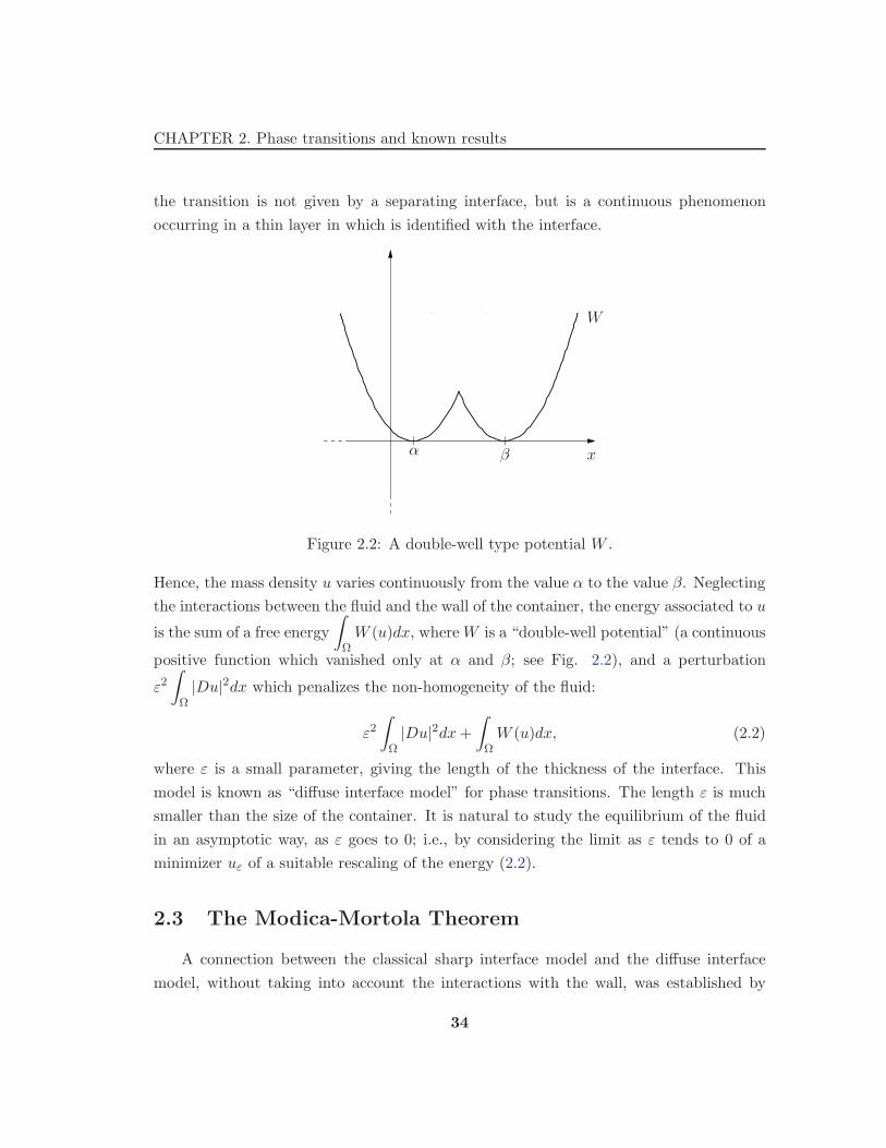
occurring in a thin layer in which is identified with the interface.
α β
W
x
Figure 2.2: A double-well type potential W .
Hence, the mass density u varies continuously from the value α to the value β. Neglecting
the interactions between the fluid and the wall of the container, the energy associated to u
is the sum of a free energy
∫
ΩW (u)dx, whereW is a “double-well potential” (a continuous
positive function which vanished only at α and β; see Fig. 2.2), and a perturbation
ε2∫
Ω|Du|2dx which penalizes the non-homogeneity of the fluid:
ε2∫
Ω|Du|2dx+
∫
ΩW (u)dx, (2.2)
where ε is a small parameter, giving the length of the thickness of the interface. This
model is known as “diffuse interface model” for phase transitions. The length ε is much
smaller than the size of the container. It is natural to study the equilibrium of the fluid
in an asymptotic way, as ε goes to 0; i.e., by considering the limit as ε tends to 0 of a
minimizer uε of a suitable rescaling of the energy (2.2).
2.3 The Modica-Mortola Theorem
A connection between the classical sharp interface model and the diffuse interface
model, without taking into account the interactions with the wall, was established by
34

CHAPTER 2. Phase transitions and known results
Modica in [48](1987). He proved that a suitable rescaling of the energy (2.2) Γ-converges
to the surface energy functional u 7→ σH2(Su); He also proved that at equilibrium the
two phases arrange themselves in order to minimize the area of the separation interface.
This result was conjectured by De Giorgi. A great contribute to the work of Modica was
already given by Modica himself and Mortola in [50] (1977).
For every ε > 0, let us consider the functional Eε defined in H1(Ω), given by the
following rescaling of (2.2)
Eε(u) := ε
∫
Ω|Du|2dx+
1
ε
∫
ΩW (u)dx. (2.3)
To explain the scale of this penalization, we show a heuristic scaling argument in dimension
one.
Consider an interval (t, t+δ) and suppose that u is close to α and β at the endpoints of
this interval, respectively. We can show that the contribution on this interval of the first
integral of (2.2) is of order ε/δ (since the gradient is of order ε), while the contribution
of the second integral is of order δ.
Hence
ε2∫ t+δ
t|u′|2ds+
∫ t+δ
tW (u)ds ∼= ε2
δ+ δ,
and the minimization in δ of this quantity gives δ = ε and a contribution of order ε. This
implies that if the energy is bounded then the number of such intervals is bounded and
hence u resembles a piecewise-constant function. This argument suggests a scaling of the
problem and to consider the minimum problem
min
ε
∫
Ω|Du|2dx+
1
ε
∫
ΩW (u)dx :
∫
Ωu dx = C
,
whose minimizers are clearly the same as the energy (2.2).
Theorem 2.1. The functional Eε : H1(Ω) → R defined by (2.3) Γ-converges with respect
to the L1(Ω) convergence to the functional
E(u) :=
σH2(Su), if u ∈ BV (Ω, α, β),+∞, otherwise,
(2.4)
where σ := 2
∫ β
αW 1/2dt.
35
CHAPTER 2. Phase transitions and known results
Since the Modica-Mortola Theorem, several results were given which extend theorem
2.1 in different directions. In particular, we are interested in the possibility of replacing
the perturbation term by a p-energy of Dirichlet. In this case, a similar heuristic argument
like in the quadratic case, gives the following rescaled energy
δp−1
∫
Ω|Du|pdx+
1
δ
∫
ΩW (u)dx.
Anyway, choosing ε such that δp−1 = εp−2 better fits to our purposes. So that, for every
open set A ⊂ R3 and every real function u ∈W 1,p(A), we consider the following functional
Gε(u,A) := εp−2
∫
A|Du|pdx+
1
εp−2p−1
∫
AW (u)dx. (2.5)
Let W be a primitive of W p/(p−1), we denote by σp :=p
(p− 1)p/(p−1)|W(β) −W(α)|.
Theorem 2.2. For every domain A ⊂ R3 the following statements hold.
(i) If (uε) ⊂ W 1,p(A) is a sequence with uniformly bounded energies Gε(uε, A). Then
(uε) is pre-compact in L1(A) and every cluster point belongs to BV (A, α, β).
(ii) For every u ∈ BV (A, α, β) and every sequence (uε) ⊂ W 1,p(A) such that uε → u
in L1(A),
lim infε→0
Gε(uε, A) ≥ σpH2(Su),
(iii) For every u ∈ BV (A, α, β) there exists a sequence (uε) ⊂ W 1,p(A) such that
uε → u in L1(A) and
lim supε→0
Gε(uε, A) ≤ σpH2(Su).
Moreover, when Su is a closed Lipschitz surface in A, the functions uε may be
required to be (CW /εp−2p−1 )-Lipschitz continuous, and to converge to u uniformly on
every set with positive distance from Su (here CW is the supremum of W 1/p in
[α, β]).
A proof can be obtained thanks to simple modifications to the proof of the Modica-
Mortola Theorem by Modica in [48] (see also [22], Theorem 3.10, p. 42). We preferred to
enunciate the results as in the Theorem 2.2, because they will be useful in this form to
our goal.
36
CHAPTER 2. Phase transitions and known results
Remark 2.3. Either in the quadratic version or in the super-quadratic one of the Modica-
Mortola functional, the optimal constant in the limit energy comes from an optimal profile
problem. For instance, in the quadratic case, we have
σ :=
∫
R
|u′|2dt+
∫
R
W (u)dt : u ∈ H1(R), limt→−∞
u(t) = α, limt→+∞
u(t) = β
. (2.6)
The minimum problem (2.6) represents the minimal cost we pay each time we have a
transition from α to β (or conversely) in the real line. Moreover, we explicitly know the
optimal profile; it is given by the solution of the following differential equation
u′ =√
W (u),
u(0) =α+ β
2;
that is, the Euler-Lagrange equation of the problem.This fact is strictly linked to the
structure of the Modica-Mortola functional, which is characterized by the “equi-partition
of the energy” between its two terms.
2.4 The interactions between the fluids and the wall of the
container
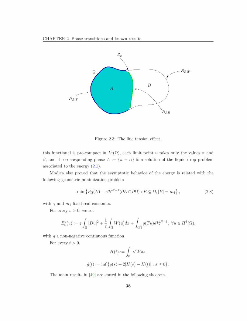
We stress that Theorem 2.1 and Theorem 2.2 do not take into account the interaction of
the fluid with the wall of the container. In this sense, an extension of the classical model
for two-phase fluids is obtained by adding to the energy (2.1) a line tension energy1
with density τ concentrated along the line Lc ≡ ∂SAW , where SAB meets the wall of the
container; i.e., along the “contact line” (see Fig. 2.3). In this model, the capillary energy
becomes
E(A) := σH2(SAB) + σAWH2(SAW ) + σBWH2(SBW ) + τH1(Lc). (2.7)
A partial rigorous connection with this classical model is provided by Modica at
the end of 80’s. In [49], Modica added to (2.3) a boundary contribution of the form
λ
∫
∂Ωg(Tu)dH2, where Tu denotes the trace of u on ∂Ω, λ does not depend on ε, and
g is a non-negative continuous function. He proved that a sequence of minimizers uε for
1In Gibbs’ original formulation, the concept of line tension was introduced to describe the excess freeenergy arising a three-phase line, that is, along a curve where three distinct phases coexist (see [41]).
37
CHAPTER 2. Phase transitions and known results
Ω
AB
SAB
Lc
SBW
SAW
Figure 2.3: The line tension effect.
this functional is pre-compact in L1(Ω), each limit point u takes only the values α and
β, and the corresponding phase A := u = α is a solution of the liquid-drop problem
associated to the energy (2.1).
Modica also proved that the asymptotic behavior of the energy is related with the
following geometric minimization problem
min
PΩ(E) + γHN−1(∂E ∩ ∂Ω) : E ⊆ Ω, |E| = m1
, (2.8)
with γ and m1 fixed real constants.
For every ε > 0, we set
Egε (u) := ε
∫
Ω|Du|2 +
1
ε
∫
ΩW (u)dx+
∫
∂Ωg(Tu)dHN−1, ∀u ∈ H1(Ω),
with g a non-negative continuous function.
For every t > 0,
H(t) :=
∫ t
0
√Wds,
g(t) := inf g(s) + 2|H(s) −H(t)| : s ≥ 0 .
The main results in [49] are stated in the following theorem.
38
CHAPTER 2. Phase transitions and known results
Theorem 2.4. [[49], Theorem 2.1, p. 497]. Fix m ∈ [α|Ω|, β|Ω|] and let (uε) ⊂ C1 be a
minimizing sequence of Egε among the class of functions with fixed volume m. If uε → u0
in L1(Ω), then
(i) W (u0(x)) = 0, a.e. x ∈ Ω;
(ii) The set E0 := x ∈ Ω : u0(x) = α is a solution of the minimum problem (2.8), with
γ :=g(α) − g(β)
2∫ βα
√Wdt
and m1 :=β|Ω| −m
β − α;
(iii) limε→0
Egε (uε) =
(
2
∫ β
α
√Wdt
)
PΩ(E0)+g(α)HN−1(∂E0∩∂Ω)+g(β)HN−1(∂Ω\∂E0).
2.5 Phase transitions with line tension effect
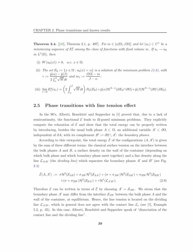
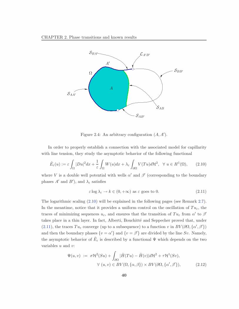
In the 90’s, Alberti, Bouchitte and Seppecher in [9] proved that, due to a lack of
semicontinuity, the functional E leads to ill-posed minimum problems. They explicitly
compute the relaxation of E and show that the total energy can be properly written
by introducing, besides the usual bulk phase A ⊂ Ω, an additional variable A′ ⊂ ∂Ω,
independent of ∂A, with its complement B′ := ∂Ω \ A′: the boundary phases.
According to this viewpoint, the total energy E of the configurations (A,A′) is given
by the sum of three different terms: the classical surface tension on the interface between
the bulk phases A and B, a surface density on the wall of the container (depending on
which bulk phase and which boundary phase meet together) and a line density along the
line LA′B′ (the dividing line) which separates the boundary phases A′ and B′ (see Fig.
2.4)
E(A,A′) := σH2(SAB) + σAWH2(SAA′) + (σ + σAW )H2(SAB′) + σBWH2(SBB′)
+(σ + σBW )H2(SBA′) + τH1(LA′B′). (2.9)
Therefore E can be written in terms of E by choosing A′ = SAW . We stress that the
boundary phase A′ may differ from the interface SAW between the bulk phase A and the
wall of the container, at equilibrium. Hence, the line tension is located on the dividing
line LA′B′ , which in general does not agree with the contact line Lc (see [9], Example
5.2, p. 35). In this case, Alberti, Bouchitte and Seppecher speak of “dissociation of the
contact line and the dividing line”.
39
CHAPTER 2. Phase transitions and known results
A
A′
Ω
SBA′
SBB′
SAA′
SAB′
SAB
LA′B′
Figure 2.4: An arbitrary configuration (A,A′).
In order to properly establish a connection with the associated model for capillarity
with line tension, they study the asymptotic behavior of the following functional
Eε(u) := ε
∫
Ω|Du|2dx+
1
ε
∫
ΩW (u)dx+ λε
∫
∂ΩV (Tu)dH2, ∀ u ∈ H1(Ω), (2.10)
where V is a double well potential with wells α′ and β′ (corresponding to the boundary
phases A′ and B′), and λε satisfies
ε log λε → k ∈ (0,+∞) as ε goes to 0. (2.11)
The logarithmic scaling (2.10) will be explained in the following pages (see Remark 2.7).
In the meantime, notice that it provides a uniform control on the oscillation of Tuε, the
traces of minimizing sequences uε, and ensures that the transition of Tuε from α′ to β′
takes place in a thin layer. In fact, Alberti, Bouchitte and Seppecher proved that, under
(2.11), the traces Tuε converge (up to a subsequence) to a function v in BV (∂Ω, α′, β′)and then the boundary phases v = α′ and v = β′ are divided by the line Sv. Namely,
the asymptotic behavior of Eε is described by a functional Ψ which depends on the two
variables u and v:
Ψ(u, v) := σH2(Su) +
∫
∂Ω|H(Tu) − H(v)|dH2 + τH1(Sv),
∀ (u, v) ∈ BV (Ω, α, β) ×BV (∂Ω, α′, β′), (2.12)
40
CHAPTER 2. Phase transitions and known results
where τ = k(β′−α′)2
π and σ := |H(β)− H(α)|, being H a primitive of 2W 1/2. Note that Ψ
reduces to (2.9) taking into account the definition of τ , σ and H, if we set σAA′ := |H(α)−H(α′)|, σAB′ := |H(α) − H(β′)|, σBA′ := |H(β) − H(α′)| and σBB′ := |H(β) − H(β′)|.
Theorem 2.5. [[9], Theorem 2.6, p. 10] Let Eε : H1(Ω) → R and Ψ : BV (Ω, α, β) ×BV (∂Ω, α′, β′) → R be defined by (2.10) and (2.12) respectively. Then
(i) If (uε) ⊂ H1(Ω) is a sequence with uniformly bounded energies Eε(uε), then the
sequence (uε, Tuε) is pre-compact in L1(Ω)×L1(∂Ω) and every cluster point belongs
to BV (Ω, α, β) ×BV (∂Ω, α′, β′).
(ii) For every (u, v) ∈ BV (Ω, α, β) × BV (∂Ω, α′, β′) and every sequence (uε) ⊂H1(Ω) such that uε → u in L1(Ω) and Tuε → v in L1(∂Ω),
lim infε→0
Eε(uε) ≥ Ψ(u, v),
(iii) For every (u, v) ∈ BV (Ω, α, β) ×BV (∂Ω, α′, β′) there exists a sequence (uε) ⊂H1(Ω) such that uε → u in L1(Ω), Tuε → v in L1(∂Ω) and
lim supε→0
Eε(uε) ≤ Ψ(u, v).
The proof of Theorem 2.5 requires several steps in which different effects are analyzed
and then different terms of the limit energy Ψ can be deduced. In the bulk term, the
limit energy can be evaluate like in [48], while the second term in Ψ is obtained by
adapting the approach by Modica in [49]. The main step in the proof concerns the analysis
of the line tension effect. Via “localization” and slicing techniques, Alberti, Bouchitte
and Seppecher reduces the analysis of the line tension to the asymptotic analysis of the
following functional defined on a two-dimensional half-disk
E2ε (u) := ε2
∫
Dr
|Du|2dx+ λε
∫
Er
V (Tu)dH1, (2.13)
where, for every r > 0, we denote by
Dr :=
(x1, x2) ∈ R2 : x2
1 + x22 < r2, x2 > 0
,
(2.14)
Er :=
(x1, x2) ∈ R2 : x2
1 + x22 < r2, x2 = 0
∼= (−r, r).
41
CHAPTER 2. Phase transitions and known results
Then the two-dimensional Dirichlet energy (2.13) is replaced on the half-disk Dr by the
H1/2 intrinsic norm on the “diameter” Er. This is possible thanks to the following lemma,
concerning with the optimal constant for the trace inequality involving the L2 norm of
the gradient of a function defined on a two-dimensional domain and the H1/2 norm of its
trace on a line.
Lemma 2.6. [[9], Corollary 6.4, p. 41]. Let u be a function in H1(Dr), then the trace of
u on the segment Er × 0 belongs to H1/2(Er) and
∫ ∫
Er×Er
∣
∣
∣
∣
Tu(t′) − Tu(t)
t′ − t
∣
∣
∣
∣
2
dt′dt ≤ 2π
∫
Dr
|Du|2dx. (2.15)
Hence, the original problem is reduced to the study of a new kind of perturbation
problem involving a non-local term. Let I be an open interval in R, for every v ∈ H1/2,
we set
E1ε (v) := ε
∫∫
I×I
∣
∣
∣
∣
v(t) − v(t′)
t− t′
∣
∣
∣
∣
2
dtdt′ + λε
∫
IV (v) dt, (2.16)
where λε satisfies the condition (2.11).
Remark 2.7. The singular perturbation problem involving the energies (2.16) brings to
the fore the right scaling for (2.10); i.e., the choice of λ such that log λε ≈ 1/ε.
Let us consider the following energy:
E1ε (v) := ε2
∫ ∫
I×I
∣
∣
∣
∣
v(t′) − v(t)
t′ − t
∣
∣
∣
∣
2
dt′dt +
∫
IV (v)dt,
on a one-dimensional set I = (a, b).
Adapting the argument in Section 2.3, we look at a transition from α′ to β′ taking
place on an interval (t, t+ δ). We then have
E1ε (v) ≥ 2ε2
∫ ∫
(a,t)×(t+δ,b)
∣
∣
∣
∣
1
s′ − s
∣
∣
∣
∣
2
ds′ds+ Cδ
≥ −2ε2(log δ + C) + Cδ.
By optimizing the last expression we get δ = 2ε2/C and hence
E1ε (v) ≥ 4ε2| log ε| +O(ε2).
42
CHAPTER 2. Phase transitions and known results
We are then led to the scaled energy
1
| log ε|
∫ ∫
I×I
∣
∣
∣
∣
v(t′) − v(t)
t′ − t
∣
∣
∣
∣
2
dt′dt+1
ε2| log ε|
∫
IV (v)dt,
and hence, by renaming ε the scaling factor 1/| log ε|, we obtain the energy (2.16).
Notice that this natural scaling signs the main differences with the classical Modica-
Mortola problem. In fact, the asymptotic behavior of the Modica-Mortola functional
(2.3) is characterized by the equi-partition of the energy between the two terms in the
functional and by a suitable scaling property which provides an optimal profile problem
describing the shape of the optimal transition. While, the logarithmic scaling for the
functionals (2.16) produces no equi-partition of the energy at all; the limit comes only
from the non-local part of the energy and any profile is optimal as far as transition occurs
in a layer of order ε.
Similar effects can be found in other recent results for phase transition problems with
non local singular perturbation (see Garroni and Muller[39] and Kurzke[46], [47]).
Alberti, Bouchitte and Seppecher analyze the asymptotic behavior of (0.11) in [8],
proving that
E1ε
Γ−→ 2k(β′ − α′)H0(Sv),
and strongly use this result to obtain the boundary term in (0.8).
Theorem 2.8. [[8], Theorem 1, p. 334, and [9], Theorem 4.4, p. 20.] Let E1ε : H1/2(I) →
R be defined by (2.16) and, for every v ∈ BV (I, α′, β′), set E1(v) := 2k(β′−α′)2H0(Sv).
Then
(i) If (vε) ⊂ H1/2(I) is a sequence such that E1ε (vε) is bounded, then (vε) is pre-compact
in L1(I) and every cluster point belongs to BV (I, α′, β′).
(ii) For every v ∈ BV (I, α′, β′) and every sequence (vε) ⊂ H1/2(I) such that vε → v
in L1(I),
lim infε→0
E1ε (vε) ≥ E1(v).
(iii) For every v ∈ BV (I, α′, β′) there exists a sequence (vε) ⊂ H1/2(I) such that
vε → v in L1(I) and
lim supε→0
E1ε (vε) ≤ E1(v).
43
Chapter 3
A singular perturbation result
with a fractional norm
We study a problem involving a non-local singular perturbation for a Cahn-Hilliard
functional of the type of the energy (2.16), seen in the previous chapter:
E1ε (v) := ε
∫∫
I×I
∣
∣
∣
∣
v(x) − v(x′)
x− x′
∣
∣
∣
∣
2
dxdx′ + λε
∫
IV (v) dx. (3.1)
Let I be an open bounded interval of R and V a non-negative continuous function
vanishing only at α′, β′ ∈ R (0 < α′ < β′), with growth at least linear at infinity. We
investigate the asymptotic behavior in terms of Γ-convergence of the following functional
Kε(v) := εp−2
∫∫
I×I
∣
∣
∣
∣
v(x) − v(x′)
x− x′
∣
∣
∣
∣
p
dxdx′ +1
ε
∫
IV (v) dx, ∀v ∈W
1− 1p,p(I), (p > 2), (3.2)
as ε→ 0.
We recall that the natural logarithmic scaling in (2.16) signs the main differences with
the classical Modica-Mortola problem and, also, with our functional (3.2). In fact, the
logarithmic scaling produces no equi-partition of the energy; all the limit comes only from
the non-local part of the energy and any profile is optimal as far as transition occurs in
a layer of order ε.
If we make the same computation seen in Chapter 2, we note that both the terms in
functional (3.2) are of the first order; i.e., both the terms are important in the limit. We
can bring out this characteristic of (3.2) in view of the following scaling property (3.5)
44
CHAPTER 3. A singular perturbation result with a fractional norm
and hence the limit is characterized by the following optimal profile problem
γ := inf
∫∫
R×R
∣
∣
∣
∣
w(x) − w(x′)
x− x′
∣
∣
∣
∣
p
dxdx′ +
∫
R
V (w) dx : w ∈W 1− 1p,p
loc (R),
limx→−∞
w(x) = α′, limx→+∞
w(x) = β′
. (3.3)
3.1 The Γ-convergence result
The asymptotic behavior in term of Γ-convergence of Kε is described by the functional
K(v) := γH0(Sv) , v ∈ BV (I, α′, β′), (3.4)
where γ is given by the optimal profile problem (3.3).
The Γ-convergence result is precisely stated in the following theorem.
Theorem 3.1. [[39], Theorem , p. 113]. LetKε : W 1− 1p,p(I) → R and K : BV (I, α′, β′) →
R be defined by (3.2) and (3.4).
Then
(i) [Compactness] If (vǫ) ⊂ W 1− 1p,p(I) is a sequence such that Kε(vǫ) is bounded,
then (vǫ) is pre-compact in L1(I) and every cluster point belongs to BV (I, α′, β′).
(ii) [Lower bound inequality] For every v ∈ BV (I, α′, β′) and every sequence
(vǫ) ⊂W 1− 1p,p(I) such that vǫ → v in L1(I),
lim infε→0
Kε(vǫ) ≥ K(v).
(iii) [Upper bound inequality] For every v ∈ BV (I, α′, β′) there exists a sequence
(vǫ) ⊂W 1− 1p,p(I) such that vǫ → v in L1(I) and
lim supε→0
Kε(vǫ) ≤ K(v).
45
CHAPTER 3. A singular perturbation result with a fractional norm
3.2 The optimal profile problem
In this section we will study the main features of our functional, namely the scaling
property and the optimal profile problem.
It is useful to introduce the localization of the functional Kε. For every open set J ⊆ I
and every function v ∈W 1− 1p,p(J) we will denote
Kε(v, J) := εp−2
∫∫
J×J
∣
∣
∣
∣
v(x) − v(x′)
x− x′
∣
∣
∣
∣
p
dxdx′ +1
ε
∫
JV (v) dx.
Clearly, Kε(v) = Kε(v, I), for every v ∈W1− 1
p,p(I).
Given J ⊆ I and v ∈ W 1− 1p,p(J) we set v(ε)(x) := v(εx) and J/ε := x : εx ∈ J. By
scaling it is immediately seen that
Kε(v, J) = K1(v(ε), J/ε). (3.5)
In view of this scaling property, it is now natural to consider the optimal profile problem
(3.3). The constant γ represents the minimal cost in the term of the non-scaled energy
K1 for a transition from α′ to β′ on the whole real line. By (3.5) γ will also give the cost
of one jump from α′ to β′.
Using the monotone rearrangement result of Section 1.4, we will prove that the infi-
mum in (3.3) is not trivial and is achieved.
We recall that the increasing rearrangement v∗ of a function v ∈ W 1− 1p,p(J), with
J = (a, b), is defined by
v∗(a+ x) := sup λ : |t ∈ (a, b) : v(t) < λ| ≤ x , ∀x ∈ (0, b − a), (3.6)
and satisfies
Kε(v∗, J) ≤ Kε(v, J) (3.7)
(see Theorem 1.14, p. 30 and Theorem 1.15, p. 30).
In order to prove the upper bound it is convenient to introduce an auxiliary optimal
profile problem. For every T > 0, we consider
γT := inf
K1(w,R) : w ∈W1− 1
p,p
loc (R), w(x) = α′ ∀x ≤ −T,w(x) = β′ ∀x ≥ T
. (3.8)
By the compactness of the embedding of W 1− 1p,p((−2T, 2T )) in Lp((−2T, 2T )), it is easy
to prove that the minimum in (3.8) is achieved. By truncation and rearrangement it
46

CHAPTER 3. A singular perturbation result with a fractional norm
also follows that the minimum can be achieved by a function ϕT ∈ W1− 1
p,p
loc (R) which is
non-decreasing and satisfies α′ ≤ ϕT ≤ β′.
Proposition 3.2. The sequence γT is non-increasing in T and limT→+∞
γT = γ.
Proof. By the definition of γT , it immediately follows that γT is monotone and is greater
than or equal to γ. Hence, the limit exists and satisfies
limT→+∞
γT ≥ γ.
It remains to prove the reverse inequality. For every µ > 0, let us fix ψ ∈ W1− 1
p,p
loc (R)
such that
limx→−∞
ψ(x) = α′, limx→+∞
ψ(x) = β′ and K1(ψ,R) ≤ γ + µ.
Moreover, by truncation we may always assume that α′ ≤ ψ ≤ β′.
The idea is to modify ψ in order to construct a function ϕ which is a good competitor
for γT . To this aim we consider
Ψ(x) :=
∫
R
∣
∣
∣
∣
ψ(x) − ψ(x′)
x− x′
∣
∣
∣
∣
p
dx′.
Since Ψ ∈ L1(R) we can choose a sequence Tnn∈N, with Tn → +∞, such that
Ψ(−Tn) → 0 and Ψ(Tn) → 0 as n→ +∞.
For every δ > 0, due to the asymptotic behavior of ψ, we can find nδ ∈ N such that
ψ(−Tn) ≤ α′ + δ and ψ(Tn) ≥ β′ − δ, ∀n ≥ nδ. (3.9)
For every M > 0, we define a function ϕ which coincides with ψ in [−Tn, Tn], satisfies
ϕ(x) = α′ if x < −Tn−M and ϕ(x) = β′ if x > Tn+M and it is affine in (−Tn−M,−Tn)and (Tn, Tn +M) (see Fig. 3.1).
47

CHAPTER 3. A singular perturbation result with a fractional norm
α′
β′
x
ψ
Figure 3.1: The competitor ϕ.
Namely,
ϕ(x) :=
α′ if x ∈ (−∞,−Tn −M ],
ψ(−Tn) − α′
M(x+ Tn) + ψ(−Tn) if x ∈ (−Tn −M,−Tn),
ψ(x) if x ∈ [−Tn, Tn],
β′ − ψ(Tn)
M(x− Tn) + ψ(Tn) if x ∈ (Tn, Tn +M),
β′ if x ∈ [Tn +M,+∞).
Clearly, ϕ is a good competitor for γTn+M . Let us compute its energy, denoting Jn :=
48

CHAPTER 3. A singular perturbation result with a fractional norm
(−Tn, Tn),
γTn+M ≤ K1(ϕ,R)
= K1(ψ, Jn) +K1(ϕ,R \ Jn) + 2
∫∫
(R\Jn)×Jn
∣
∣
∣
∣
ϕ(x) − ϕ(x′)
x− x′
∣
∣
∣
∣
p
dxdx′
≤ γ + µ+
∫∫
(R\Jn)×(R\Jn)
∣
∣
∣
∣
ϕ(x) − ϕ(x′)
x− x′
∣
∣
∣
∣
p
dxdx′ +
∫
R\Jn
V (ϕ) dx
+2
∫∫
(R\Jn)×Jn
∣
∣
∣
∣
ϕ(x) − ϕ(x′)
x− x′
∣
∣
∣
∣
p
dxdx′
= γ + µ+ I1 + I2 + I3. (3.10)
The first two integrals in the right hand side of (3.10) can be easily estimated as follows
I1 :=
∫∫
(R\Jn)×(R\Jn)
∣
∣
∣
∣
ϕ(x) − ϕ(x′)
x− x′
∣
∣
∣
∣
p
dxdx′ ≤ 2(β′ − α′)p∫ −Tn
−∞
∫ +∞
Tn
dxdx′
|x− x′|p
=(β′ − α′)p
(p− 1)(p − 2)(2Tn)p−2
and
I2 :=
∫
R/Jn
V (ϕ) dx ≤ 2Mωδ,
where
ωδ := maxs∈[α′,α′+δ]∪[β′−δ,β′]
V (s). (3.11)
Instead, an upper bound for the last integral requires more attention in computation. Let
us show it in detail.
I3 := 2
∫ −Tn−M
−∞
∫ Tn
−Tn
∣
∣
∣
∣
ϕ(x) − ϕ(x′)
x− x′
∣
∣
∣
∣
p
dxdx′ + 2
∫ −Tn
−Tn−M
∫ Tn
−Tn
∣
∣
∣
∣
ϕ(x) − ϕ(x′)
x− x′
∣
∣
∣
∣
p
dxdx′
+2
∫ +∞
Tn+M
∫ Tn
−Tn
∣
∣
∣
∣
ϕ(x) − ϕ(x′)
x− x′
∣
∣
∣
∣
p
dxdx′ + 2
∫ Tn+M
Tn
∫ Tn
−Tn
∣
∣
∣
∣
ϕ(x) − ϕ(x′)
x− x′
∣
∣
∣
∣
p
dxdx′.
49
CHAPTER 3. A singular perturbation result with a fractional norm
We have
2
∫ −Tn−M
−∞
∫ Tn
−Tn
∣
∣
∣
∣
ϕ(x) − ϕ(x′)
x− x′
∣
∣
∣
∣
p
dxdx′ = 2
∫ −Tn−M
−∞
∫ Tn
−Tn
∣
∣
∣
∣
ψ(x′) − α′
x− x′
∣
∣
∣
∣
p
dxdx′
≤ 2(β′ − α′)p∫ −Tn−M
−∞
∫ Tn
−Tn
dxdx′
|x− x′|p
=2(β′ − α′)p
(p− 1)(p − 2)Mp−2.
Moreover
2
∫ −Tn
−Tn−M
∫ Tn
−Tn
∣
∣
∣
∣
ϕ(x) − ϕ(x′)
x− x′
∣
∣
∣
∣
p
dxdx′
= 2
∫ −Tn
−Tn−M
∫ Tn
−Tn
∣
∣
∣ψ(x′) − ψ(−Tn) − ψ(−Tn)−α′
M (x+ Tn)∣
∣
∣
p
|x− x′|p dxdx′
≤ 2p∫ −Tn
−Tn−MΨ(−Tn)dx+ 2p
|ψ(−Tn) − α′|pMp
∫ −Tn
−Tn−M
∫ Tn
−Tn
∣
∣
∣
∣
x+ Tnx− x′
∣
∣
∣
∣
p
dxdx′
≤ 2pMΨ(−Tn) +2p−1δp
(p− 1)Mp−2, ∀n ≥ nδ ,
where we used that
∫ −Tn
−Tn−M
∫ Tn
−Tn
|x+ Tn|p|x− x′|p dxdx
′ =1
p− 1
∫ −Tn
−Tn−M
(
|x+ Tn| −|x+ Tn|p|Tn − x|p−2
)
dx
≤ M2
2(p − 1).
Similarly, we can estimate the third and the fourth integrals of I3 and we get
I3 ≤ 2pM(Ψ(−Tn) + Ψ(Tn)) +2pδp
(p− 1)Mp−2+
4(β′ − α′)p
(p− 1)(p − 2)Mp−2.
Finally, by (3.10), we obtain
γTn+M ≤ γ + µ+ rn + rδ +4(β′ − α′)p
(p− 1)(p − 2)Mp−2, ∀n ≥ nδ, (3.12)
50
CHAPTER 3. A singular perturbation result with a fractional norm
where
rn :=2(β′ − α′)p
(p− 1)(p − 2)(2Tn)p−2+ 2pM (Ψ(−Tn) + Ψ(Tn))
and
rδ :=2p
(p− 1)Mp−2δp + 2Mωδ.
Taking the limit as n→ +∞ and then δ → 0 and M → +∞, we get
limT→+∞
γT = limn→+∞
γTn+M ≤ γ + µ,
which concludes the proof by the arbitrariness of µ.
Let us conclude this section with the proof of the existence of an optimal profile.
Proposition 3.3. The minimum for γ defined by (3.3) is achieved by a non-decreasing
function ϕ satisfying α′ ≤ ϕ ≤ β′.
Proof. Let T > 0 and let ϕT be a non-decreasing minimizer for γT . Since the functions
ϕT are monotone and bounded, by Helly’s Theorem, there exist a subsequence ϕTk of ϕT
and a non-decreasing function ϕ, bounded by α′ and β′, such that ϕTk converges pointwise
in R to ϕ. By Fatou’s Lemma and Proposition 3.2 we also have
∫∫
R×R
∣
∣
∣
∣
ϕ(x′) − ϕ(x′)
x− x′
∣
∣
∣
∣
p
dxdx′ +
∫
R
V (ϕ) dx ≤ limk→∞
γTk = γ .
This implies that ϕ is a minimizer for γ. 2
3.3 Compactness
The proof of the compactness follows the lines of the proof of Alberti, Bouchitte and
Seppecher in [8], requiring a Young measure argument. We use the following lemma which
gives a (non-optimal) lower bound for Kε.
Lemma 3.4. Let (vǫ) ⊂ W 1− 1p,p(I) and let J ⊂ I be an open interval. For every δ such
that 0 < δ < (β′ − α′)/2, let us define
Aε := x ∈ I : vǫ(x) ≤ α′ + δ and Bε := x ∈ I : vǫ(x) ≥ β′ − δ.
51
CHAPTER 3. A singular perturbation result with a fractional norm
Let us set
aε :=|Aε ∩ J |
|J | and bε :=|Bε ∩ J |
|J | . (3.13)
Then
Kε(vǫ, J) ≥(
2(β′ − α′ − 2δ)p
(p − 1)(p − 2)|J |p−2
(
1 − 1
(1 − aε)p−2− 1
(1 − bε)p−2
))
εp−2 + cδ, (3.14)
where cδ does not depend on ε.
Proof. Let x0, x′0 ∈ R be such that J = (x0, x
′0); we obtain
Kε(vε, J) ≥ Kε(v∗ε , J)
≥ 2εp−2(β′ − α′ − 2δ)p∫ x0+aε|J |
x0
∫ x′0
x′0−bε|J |
dxdx′
|x− x′|p +1
εmδ|J |(1 − aε − bε)
=2εp−2(β′ − α′ − 2δ)p
(p− 1)(p − 2)|J |p−2
(
1 − 1
(1 − aε)p−2− 1
(1 − bε)p−2+
1
(1 − aε − bε)p−2
)
+1
εmδ|J |(1 − aε − bε),
where v∗ε denote the non-decreasing rearrangement of vε in (x0, x′0) defined by (3.6) and
mδ := minV (s) : α′ + δ ≤ s ≤ β′ − δ.Minimizing with respect to |J |(1 − aε − bε), we get
Kε(vε, J) ≥ εp−2
(
2(β′ − α′ − 2δ)p
(p− 1)(p − 2)|J |p−2
(
1 − 1
(1 − aε)p−2− 1
(1 − bε)p−2
))
+21
p−1(p− 1)
p−2p−1
p− 2(β′ − α′ − 2δ)
pp−1m
p−2p−1
δ ,
for every 0 < δ < (β′ − α′)/2, and hence (3.14) is proved.
We are now in a position to prove the compactness result (i.e., Theorem 3.1(i)).
Let (vǫ) ⊂ W 1−1/p,p(I) be a sequence with equi-bounded energy; i.e., a sequence
satisfying supε>0
Kε(vǫ) ≤ C. In particular
∫
IV (vǫ) dx ≤ Cε (3.15)
and this implies that
V (vǫ) → 0 in L1(I). (3.16)
52

CHAPTER 3. A singular perturbation result with a fractional norm
Thanks to the growth assumptions on V , (vǫ) is equi-integrable. Hence, by Dunford-
Pettis’ Theorem, (vǫ) is weakly relatively compact in L1(I); i.e., there exists v ∈ L1(I)
such that (up to subsequences) (vǫ) v in L1(I)
We have to prove that this convergence is strong in L1(I) and that v ∈ BV (I, α, β).Let νx be the Young measure associated to (vǫ). Since V ≥ 0, we can use Theorem 1.5
(see Section 1.2, p. 24). We have∫
I
∫
R
V (t) dνx(t) ≤ lim infε→0
∫
IV (vε) dx
Hence, by (3.16), it follows that∫
R
V (t) dνx(t) = 0, a.e. x ∈ I,
which implies the existence of a function ϑ on [0, 1] such that
νx(dt) = ϑ(x)δα′(dt) + (1 − ϑ(x))δβ′(dt) , x ∈ I
and
v(x) = ϑ(x)α′ + (1 − ϑ(x))β′ , x ∈ I.
It remains to prove that ϑ belongs to BV (I, 0, 1). Let us consider the set Sϑ of
the points where the approximate limits of ϑ is neither 0 nor 1. For every N ≤ H0(Sϑ)
we can find N disjoint intervals Jnn=1,...,N such that Jn ∩ Sϑ 6= ∅ and such that the
quantities anε and bnε , defined by (3.13) replacing J by Jn, satisfy
anε → an ∈ (0, 1) and bnε → bn ∈ (0, 1) as ε goes to zero.
We can now apply Lemma 3.4 in the interval Jn and, taking the limit as ε → 0 in the
inequality (3.14), we obtain
lim infε→0
Kε(uε, Jn) ≥ cδ.
Finally, we use the sub-additivity of Kε(u, ·) and we get
lim infε→0
Kε(vǫ, I) ≥N∑
n=1
lim infKε(vǫ, Jn) ≥ Ncδ. (3.17)
Since (vǫ) has equi-bounded energy, this implies that Sϑ is a finite set and, since a function
w : I → 0, 1 is in BV (I, 0, 1) if and only if H0(Sw) <∞, it follows θ ∈ BV (I, 0, 1).The proof of the compactness for Kε is complete.
53
CHAPTER 3. A singular perturbation result with a fractional norm
3.4 Lower bound inequality
In this section, we prove the Γ-liminf inequality. An optimal lower bound for Kε(vǫ)
is a consequence of the following proposition.
Proposition 3.5. Let J be an open interval of R. Let (vǫ) be a sequence of non-decreasing
functions in W 1− 1p,p(J) and assume that there exist a, b ∈ J , a < b, such that for every
δ > 0 there exists εδ such that
vǫ(a) ≤ α′ + δ and vǫ(b) ≥ β′ − δ ∀ε ≤ εδ.
Then
lim infε→0
Kε(vε, J) ≥ γ.
Proof. Let J = (a, b). It is clearly enough to consider the case
lim infε→0
Kε(vǫ, (a, b)) < +∞.
By a truncation argument, without loss of generality, we may also assume that
α′ ≤ vǫ(x) ≤ β′, ∀x ∈ (a, b).
Let us define
Uε(x) := εp−2
∫ b
a
∣
∣
∣
∣
vǫ(x) − vǫ(x′)
x− x′
∣
∣
∣
∣
p
dx′.
By the fact that
lim infε→0
∫ b
aUε(x) dx
is finite, we get that there exist x ∈ (a, a) and x′ ∈ (b, b) such that
lim infε→0
Uε(x) ≤ C and lim infε→0
Uε(x′) ≤ C for some C > 0. (3.18)
54
CHAPTER 3. A singular perturbation result with a fractional norm
Fix M > 0. We now extend vǫ on the whole R as follows
vǫ(x) :=
α′ if x ∈ (−∞, x−Mε),
vǫ(x) − α′
Mε(x− x) + vǫ(x) if x ∈ [x−Mε, x],
vǫ(x) if x ∈ (x, x′),
β′ − vǫ(x′)
Mε(x− x′) + vǫ(x
′) if x ∈ [x′, x′ +Mε],
β′ if x ∈ (x′ +Mε,+∞).
Denote J := (x, x′) ⊆ (a, b). We have
Kε(vǫ, J) ≥ γ −Kε(vǫ,R \ J) − 2εp−2
∫∫
(R\J)×J
∣
∣
∣
∣
vǫ(x) − vǫ(x′)
x− x′
∣
∣
∣
∣
p
dxdx′
= γ − εp−2
∫∫
(R\J)×(R\J)
∣
∣
∣
∣
vǫ(x) − vǫ(x′)
x− x′
∣
∣
∣
∣
p
dxdx′ − 1
ε
∫
R\JV (vǫ) dx
−2εp−2
∫∫
(R\J)×J
∣
∣
∣
∣
vǫ(x) − vǫ(x′)
x− x′
∣
∣
∣
∣
p
dxdx′
= γ − I1 − I2 − I3. (3.19)
Using the definition of vǫ, we easily get
I1 := εp−2
∫∫
(R\J)×(R\J)
∣
∣
∣
∣
vǫ(x) − vǫ(x′)
x− x′
∣
∣
∣
∣
p
dxdx′
≤ εp−2(β′ − α′)p∫∫
(R\J)×(R\J)
dxdx′
|x− x′|p
=(β′ − α′)p
(p− 1)(p − 2)|J |p−2εp−2.
Moreover, since vǫ is non-decreasing,
vǫ(x) ≤ α′ + δ ∀ x ≤ a and vǫ(x) ≥ β′ − δ ∀ x ≥ b
55
CHAPTER 3. A singular perturbation result with a fractional norm
and, in particular,
I2 :=1
ε
∫
R\JV (vǫ) dx ≤ 2Mωδ,
where ωδ is defined in (3.11).
Finally, using the fact that vǫ(x) ≤ α′ + δ and vǫ(x′) ≥ β′ − δ, we can estimate the
third integral
I3 := 2εp−2
∫∫
(R\J)×J
∣
∣
∣
∣
vǫ(x) − vǫ(x′)
x− x′
∣
∣
∣
∣
p
dxdx′ = 2εp−2
∫ x−Mε
−∞
∫ x′
x
∣
∣
∣
∣
vǫ(x) − vǫ(x′)
x− x′
∣
∣
∣
∣
p
dxdx′
+2εp−2
∫ x
x−Mε
∫ x′
x
∣
∣
∣
∣
vǫ(x) − vǫ(x′)
x− x′
∣
∣
∣
∣
p
dxdx′ + 2εp−2
∫ +∞
x′+Mε
∫ x′
x
∣
∣
∣
∣
vǫ(x) − vǫ(x′)
x− x′
∣
∣
∣
∣
p
dxdx′
+2εp−2
∫ x′+Mε
x′
∫ x′
x
∣
∣
∣
∣
vǫ(x) − vǫ(x′)
x− x′
∣
∣
∣
∣
p
dxdx′. (3.20)
We have
2εp−2
∫ x−Mε
−∞
∫ y
x
∣
∣
∣
∣
vǫ(x) − vǫ(x′)
x− y
∣
∣
∣
∣
p
dxdy ≤ 2εp−2(β′ − α′)p∫ x−Mε
−∞
∫ y
x
dxdy
|x− y|p
≤ 2(β′ − α′)p
(p− 1)(p − 2)Mp−2.
Moreover,
2εp−2
∫ x
x−Mε
∫ x′
x
∣
∣
∣
∣
vǫ(x) − vǫ(x′)
x− x′
∣
∣
∣
∣
p
dxdx′
= 2εp−2
∫ x
x−Mε
∫ x′
x
|vǫ(x′) − vǫ(x) − vǫ(x)−α′
Mε (x− x)|p|x− x′|p dxdx′
≤ 2p∫ x
x−MεUε(x)dx+ 2p
|vǫ(x) − α′|pMpε2
∫ x
x−Mε
∫ x′
x
|x− x|p|x− x′|p dxdx
′
≤ 2pMεUε(x) +2p−1δp
(p− 1)Mp−2, ∀ ε ≤ εδ ,
where we used the fact that
∫ x
x−Mε
∫ x′
x
|x− x|p|x− x′|pdxdx
′ =1
(p− 1)
∫ x
x−Mε
(
|x− x| − |x− x|p|x′ − x|p−1
)
dx ≤ (Mε)2
2(p− 1).
56
CHAPTER 3. A singular perturbation result with a fractional norm
Similarly, we can estimate the third and the fourth integrals of I3 and we get
I3 ≤ 2pM(Uε(x) + Uε(y))ε+2pδp
(p− 1)Mp−2+
4(β′ − α′)p
(p− 1)(p − 2)Mp−2, ∀ ε ≤ εδ.
Hence, by (3.19), we obtain
Kε(vǫ, J) ≥ γ −(
(β′ − α′)p
(p − 1)(p − 2)|J |p−2εp−2 + 2pM(Uε(x) + Uε(y))ε − rδ
)
− 4(β′ − α′)p
(p− 1)(p − 2)Mp−2, ∀ ε ≤ εδ ,
with
rδ :=2pδp
(p− 1)Mp−2δp + 2Mωδ
vanishing as δ → 0.
Thus, by (3.18) and taking the liminf as ε→ 0 and then as δ → 0, we get
lim infε→0
Kε(vǫ, J) ≥ γ − 4(β′ − α′)p
(p− 1)(p − 2)Mp−2,
which concludes the proof by the arbitrariness of M .
Remark 3.6. Clearly an analogue proposition holds in the case of vǫ non-increasing
satisfying the hypotheses with a > b.
In order to conclude, let us first observe that, thanks to the compactness result for Kε,
we may assume that the sequence (vǫ) converges in L1(I) to some u ∈ BV (I, α′, β′).Hence, the jump set Sv is finite and we can find N := H0(Sv) disjoint subintervals
Iii=1,...,N such that Sv ∩ Ii 6= ∅, for every i = 1, ..., N .
Now, let us consider the monotone rearrangement v∗ε,i of vǫ in Ii. The rearrangement
v∗ε,i is non-decreasing if u is non-decreasing in Ii and non-increasing otherwise. With
this choice clearly v∗ε,i converges to v in L1(Ii) and thus it satisfies the assumptions of
Proposition 3.5 (see also Remark 3.6) with J replaced by Ii. Then, for every i = 1, ..., N ,
we may conclude that
lim infε→0
Kε(vǫ, Ii) ≥ lim infε→0
Kε(v∗ε,i, Ii) ≥ γ.
57
CHAPTER 3. A singular perturbation result with a fractional norm
Finally, using the sub-additivity of Kε(vǫ, ·), we get
lim infε→0
Kε(vǫ, I) ≥ lim infε→0
N∑
i=1
Kε(vǫ, Ii) ≥ Nγ = γH0(Sv)
and hence the lower bound stated by Theorem 3.1, (ii), is proved. 2
3.5 Upper bound inequality
In this section, we conclude the proof of the Theorem 3.1, proving the limsup inequality.
Let us first construct an optimal sequence for v of the form
v(x) =
α′, if x ≤ x0,
β′, if x > x0.
Let T > 0 be fixed and let ϕT ∈W1− 1
p,p
loc (R) be the minimizer for γT defined by (3.8);
i.e.,
ϕT (x) = α′ ∀ x ≤ −T, ϕT (x) = β′ ∀ x ≥ T and K1(ϕ,R) = γT .
Let us define, for every ε > 0, vǫ(x) := ϕT(
x− x0
ε
)
, for every x ∈ I. We have
vǫ → v in L1(I)
and
Kε(vǫ) = εp−2
∫∫
I×I
∣
∣
∣
∣
∣
ϕT (x−x0ε ) − ϕT (x
′−x0ε )
x− x′
∣
∣
∣
∣
∣
p
dxdx′ +1
ε
∫
IV
(
ϕT(
x− x0
ε
))
dx
= K1(ϕT , (I − x0)/ε) ≤ K1(ϕ
T ,R) = γT . (3.21)
By Proposition 3.2 we get
limT→+∞
lim supε→0
Kε(vǫ) ≤ γ.
Then by a diagonalization argument we can construct a sequence vǫ converging to v in
L1(I), which satisfies
lim supε→0
Kε(vǫ) ≤ γ.
58
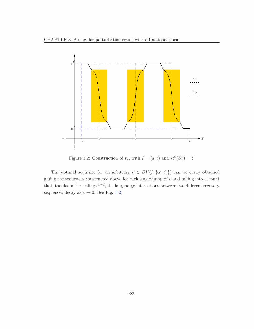
CHAPTER 3. A singular perturbation result with a fractional norm
α′
β′
a bx
vε
v
Figure 3.2: Construction of vε, with I = (a, b) and H0(Sv) = 3.
The optimal sequence for an arbitrary v ∈ BV (I, α′, β′) can be easily obtained
gluing the sequences constructed above for each single jump of v and taking into account
that, thanks to the scaling εp−2, the long range interactions between two different recovery
sequences decay as ε→ 0. See Fig. 3.2.
59
Chapter 4
A class of phase transition
problems with line tension effect
In this chapter, we introduce the main problem of this thesis, that concerns the study
of a functional similar to (2.10), but with a super-quadratic growth in the perturbation
term.
Let Ω be a bounded open subset of R3 with smooth boundary; let W and V be non-
negative continuous functions on R with growth at least linear at infinity and vanishing
respectively only in the “double well” α, β, with α < β, and α′, β′, with α′ < β′. We
also suppose that W and V are convex near their respective wells. Let p > 2 be a real
number, for every ε > 0, we consider the functional Fε defined in W 1,p(Ω), given by
Fε(u) := εp−2
∫
Ω|Du|pdx+
1
εp−2p−1
∫
ΩW (u)dx+
1
ε
∫
∂ΩV (Tu)dH2, (4.1)
where as usual Tu denotes the trace of u on ∂Ω.
Note that the choice of the scaling in (4.1) comes from the super-quadratic version of
the Modica-Mortola functional; i.e.,
εp−1
∫
Ω|Du|pdx+
1
ε
∫
ΩW (u)dx,
but we also take into account the scaling of the functional Kε studied in the previous
chapter
εp−2
∫∫
I×I
∣
∣
∣
∣
v(t) − v(t′)
t− t′
∣
∣
∣
∣
p
dtdt′ +1
ε
∫
IV (v) dt.
We analyze the asymptotic behavior of the functional Fε in terms of Γ-convergence.
Let (uε) be an equi-bounded sequence for Fε; i.e., there exists a constant C such that
60
CHAPTER 4. A class of phase transition problems with line tension effect
F (uε) ≤ C. We observe that the term1
εp−2p−1
∫
ΩW (uε)dx forces uε to take values close
to α and β, while the term εp−2
∫
Ω|Duε|pdx penalizes the oscillations of uε. We will see
that when ε tends to 0, the sequence (uε) converges (up to a subsequence) to a function
u, that belongs to BV (Ω), which takes only the values α and β. Moreover each uε has a
transition from the value α to the value β in a thin layer close to the surface Su, which
separates the bulk phases u = α and u = β. Similarly, the boundary term of Fε forces
the traces Tuε to take values close to α′ and β′, and the oscillations of the traces Tuε
are again penalized by the integral εp−2
∫
Ω|Duε|pdx. Then, we expect that the sequence
(Tuε) converges to a function v in BV (∂Ω) which takes only the values α′ and β′, and
that a concentration of energy occurs along the line Sv, which separates the boundary
phases v = α′ and v = β′.In view of possible “dissociation of the contact line and the dividing line”, we recall
that Tu may differ from v.1 Since the total energy Fε(uε) is partly concentrated in a thin
layer close to Su (where uε has a transition from α to β), partly in a thin layer close to
the boundary (where uε has a transition from Tu to v), and partly in the vicinity of Sv
(where Tuε has a transition from α′ to β′), we expect that the limit energy is the sum of
a surface energy concentrated on Su, a boundary energy on ∂Ω (with density depending
on the gap between Tu and v), and a line energy concentrated along Sv.
The asymptotic behavior of the functional Fε is described by a functional Φ which
depends on the two variables u and v. Let W be a primitive of W (p−1)/p. For every
(u, v) ∈ BV (Ω, α, β) ×BV (∂Ω, α′, β′), we will prove that
Φ(u, v) := σpH2(Su) + cp
∫
∂Ω|W(Tu) −W(v)|dH2 + γpH1(Sv), (4.2)
where as usual the jump sets Su and Sv are the complement of the set of Lebesgue
points of u and v, respectly; cp and σp are the constants defined in Chapter 2; that are,
cp :=p
(p− 1)p/(p−1); σp := cp|W(β) −W(α)|; γp is given by the optimal profile problem
γp := inf
∫
R2+
|Du|pdx+
∫
R
V (Tu)dH1 : u ∈ L1loc(R
2+) :
∫
R2+
|Du|pdx is finite,
limt→−∞
Tu(t)=α′, limt→+∞
Tu(t)=β′
. (4.3)
1See Chapter 2, p. 39.
61
CHAPTER 4. A class of phase transition problems with line tension effect
The main convergence result is precisely stated in the following theorem.
Theorem 4.1. Let Fε : W 1,p(Ω) → R and Φ : BV (Ω, α, β) × BV (∂Ω, α′, β′) → R
defined by (6.1) and (6.2).
Then
(i) [Compactness] If (uε) ⊂ W 1,p(Ω) is a sequence such that Fε(uε) is bounded,
then (uε, Tuε) is pre-compact in L1(Ω) × L1(∂Ω) and every cluster point belongs
to BV (Ω, α, β) ×BV (∂Ω, α′, β′).
(ii) [Lower Bound Inequality] For every (u, v) ∈ BV (Ω, α, β)×BV (∂Ω, α′, β′)and every sequence (uε) ⊂ W 1,p(Ω) such that uε → u in L1(Ω) and Tuε → v in
L1(∂Ω),
lim infε→0
Fε(uε) ≥ Φ(u, v).
(iii) [Upper Bound Inequality] For every (u, v) ∈ BV (Ω, α, β)×BV (∂Ω, α′, β′)there exists a sequence (uε) ⊂ W 1,p(Ω) such that uε → u in L1(Ω), Tuε → v in
L1(∂Ω) and
lim supε→0
Fε(uε) ≤ Φ(u, v).
We can easily rewrite this theorem in term of Γ-convergence. To this aim, we extend
each Fε to +∞ on L1(Ω)\W 1,p(Ω) and, from Theorem 4.1, we briefly deduce the following
remark.
Remark 4.2. Fε Γ-converges on L1(Ω) to F , given by
F (u) :=
inf Φ(u, v) : v ∈ BV (∂Ω, α′, β′) if u ∈ BV (Ω, α, β),+∞ elsewhere in L1(Ω).
Note that the limit functional Φ is of the same type of the functional Ψ (defined by
(2.12), Γ-limit of Eε. Nevertheless, the variation of the power of the gradient in the
perturbation term is not a simple generalization with respect to the quadratic case. The
structure of these two problems is different. In the quadratic case, the natural scaling
of the energy is logarithmic: this implies that the profile in which the phase transition
occurs on the boundary is not important for the first order of energy. Instead, the super-
quadratic case is characterized by an optimal profile problem which determines the line
tension in the limit. In view of this, some arguments in the proof of Theorem 4.1 will be
simplified, some other will require more care.
62
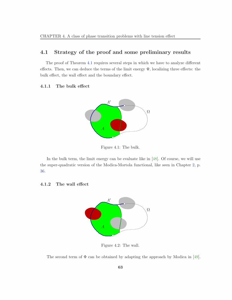
CHAPTER 4. A class of phase transition problems with line tension effect
4.1 Strategy of the proof and some preliminary results
The proof of Theorem 4.1 requires several steps in which we have to analyze different
effects. Then, we can deduce the terms of the limit energy Ψ, localizing three effects: the
bulk effect, the wall effect and the boundary effect.
4.1.1 The bulk effect
A
A′
Ω
Figure 4.1: The bulk.
In the bulk term, the limit energy can be evaluate like in [48]. Of course, we will use
the super-quadratic version of the Modica-Mortola functional, like seen in Chapter 2, p.
36.
4.1.2 The wall effect
A
A′
Ω
Figure 4.2: The wall.
The second term of Φ can be obtained by adapting the approach by Modica in [49].
63

CHAPTER 4. A class of phase transition problems with line tension effect
We recall that the results by Modica concern a Cahn-Hilliard functional with quadratic
growth in the singular perturbation term and with a boundary contribution of the form
λ
∫
∂Ωg(Tu)dH2, with λ not depending on ε and g a positive continuous function. Hence,
we need to adapt part of Proposition 1.2 ([49], p. 492) and Proposition 1.4 ([49], p. 494)
to our goal.
For every open set A ⊂ R3 and every real function u ∈ W 1,p(A), we consider the
functional
Gε(u,A) := εp−2
∫
A|Du|pdx+
1
εp−2p−1
∫
AW (u)dx. (4.4)
Proposition 4.3. For every domain A ⊂ R3 with boundary piecewise of class C1 and for
every A′ ⊂ ∂A with Lipschitz boundary, the following statements hold.
(i) For every (u, v) ∈ BV (A, α, β) × BV (A′, α′, β′) and every sequence (uε) ⊂W 1,p(A) such that uε → u in L1(A) and Tuε → v in L1(A′),
lim infε→0
Gε(uε, A) ≥ cp
∫
A′
|W(Tu) −W(v)|dH2.
(ii) Let a function v, constant on A′, and a function u, constant on A, such that u ≡ α
or u ≡ β, be given. Then there exists a sequence (uε) such that Tuε = v on A′, uε
converges uniformly to u on every set with positive distance from A′ and
lim supε→0
Gε(uε, A) ≤ cp
∫
A′
|W(Tu) −W(v)|dH2.
Moreover, the function uε may be required to beC ′W
ε(p−2)/(p−1)-Lipschitz continuous
(where C ′W is the maximum of W (1)/p over any interval which contains the values
of u and v).
Proof. We may assume that Gε(uε) ≤ C. For every ε > 0, let us denote by
wε(x) := (W uε)(x), ∀x ∈ A. (4.5)
Step 1:
∫
A|Dwε|dx ≤ constant.
64
CHAPTER 4. A class of phase transition problems with line tension effect
By Young’s Inequality, we have:∫
A|Dwε|dx =
∫
A|W ′(uε)||Duε|dx
=
∫
AW
p−1p (uε)|Duε|dx (4.6)
≤ Gε(uε)
cp≤ C
cp.
Step 2: wε → W u ∈ BV (A) in L1(A).
For every ε > 0 let us define the function
wε(x) := wε(x) − θε, ∀x ∈ A,
where
θε :=1
|A|
∫
Awεdx.
Then (see [10], Theorem 3.44, p. 148) there exists a constant cA, depending on A, such
that∫
A|wε|dx ≤ cA
∫
A|Dwε|dx. (4.7)
Since∫
A|Dwε|dx =
∫
A|Dwε|dx,
by (4.6), we obtain∫
A|Dwε|dx < const. (4.8)
By (4.7) and (4.8) follows that the sequence (wε) is bounded in W 1,1(A). Hence, by
Rellich’s Theorem, there exists a function w ∈ BV (A) such that (up to a subsequence)
wε → w in L1(A).
Since wε is bounded, it is not restrictive to assume that both (wε) and (wε) converge
almost everywhere in A, so we have that θε converges to θ in R, and, finally, that (wε)
converges to w+θ in L1(A). Thus, since uε converges to u in L1(A), by (4.5), we conclude
that (wε) converges to W u in L1(A).
65
CHAPTER 4. A class of phase transition problems with line tension effect
Moreover, by lower semicontinuity, we have
∫
A|D(W u)(x)| ≤ lim inf
ε→0
∫
A|Dwε(x)| ≤ const.
Step 3: G0(z) :=
∫
A|Dz(x)|+
∫
∂A|Tz−W(v)|dH2 is l.s.c. on BV (A) with respect to the
topology L1(A).
Let us fix z ∈ BV (A) and let (zε) be a sequence in BV (A) converging to z in L1(A). We
will prove that
lim supε→0
(G0(z) −G0(zε)) ≤ 0, (4.9)
where
G0(z) :=
∫
A|Dz(x)| +
∫
∂A|Tz −W(v)|dH2, ∀z ∈ BV (A). (4.10)
We can estimate the boundary part of the functional (4.10) with the L1-norm of the
difference of the traces fo z and zε:
∫
∂A|Tz −W(v)|dH2 −
∫
∂A|Tzε −W(v)|dH2 ≤
∫
∂A|Tz − Tzε|dH2.
Thus, we have
G0(z) −G0(zε) ≤∫
A|Dz|dx−
∫
A|Dzε(x)| +
∫
∂A|Tz − Tzε|dH2. (4.11)
For every δ > 0, take a cut-off function ξδ ∈ C∞0 (A) such that 0 ≤ ξδ(x) ≤ 1, ξδ(x) = 1 if
dist(x, ∂A) ≥ δ, |Dξδ| ≤ 2/δ.
Let us define
zδε(x) := (1 − ξδ(x))(z − zε), ∀x ∈ A,
Applying to zδε the trace inequality for BV functions by Anzellotti and Giaquinta (see
[11], Teorema 5, p. 13); we obtain
∫
∂A|Tz − Tzε|dH2 ≤
∫
Aδ
|D(z − zε)(x)| +(
2
δ+ c′
)∫
Aδ
|z − zε|dx, (4.12)
where Aδ := x ∈ A : dist(x, ∂A) ≤ δ and c is a constant that does not depend on δ.
Moreover,∫
Aδ
|D(z − zε)(x)| ≤∫
Aδ
|Dz(x)| +∫
Aδ
|Dzε(x)|, (4.13)
66
CHAPTER 4. A class of phase transition problems with line tension effect
where we used that (z − zε) ∈ BV (A). Then we have
∫
∂(Acδ)|D(z − zε)(x)| (for every ε > 0),
Hence, from (4.11), (4.12) and (4.13), we obtain
G0(z) −G0(zε) ≤∫
A|Dz(x)| +
∫
Aδ
|Dz(x)| −∫
Acδ
|Dzε(x)| +(
2
δ+ c′
)∫
Aδ
|z − zε|dx
= 2
∫
Aδ
|Dz(x)| +∫
Acδ
|Dz(x)| −∫
Acδ
|Dzε(x)| +(
2
δ+ c′
)∫
Aδ
|z − zε|dx
Finally, using the lower semicontinuity in L1(A) of the functional
z 7→∫
Acδ
|Dz(x)|
and the fact that zε converges to z in L1(A), we conclude that
lim supε→0
(G0(z) −G0(zε)) ≤ 2
∫
Aδ
|Dz(x)| (4.14)
for almost every δ > 0. By taking δ → 0 in (4.14), we obtain the inequality (4.9).
Step 4: Proof of Statement (i).
Applying the lower semicontinuity of the functional G0 to the sequence (wε) defined by
(4.5), we obtain the following inequality
cp
∫
A|D(W u)(x)| + cp
∫
∂A|W(Tu) −W(v)|dH2
≤ lim infε→0
cp
(∫
A|D(W uε)(x)| +
∫
∂A|W(Tuε) −W(v)|dH2
)
(4.15)
≤ lim infε→0
(
Gε(uε) + cp
∫
∂A|W(Tuε) −W(v)|dH2
)
.
Since Tuε → v in L1(A′), we deduce that
limε→0
cp
∫
∂A|W(Tuε) −W(v)|dH2 = 0. (4.16)
Hence, the lower bound inequality of statement (i) follows from (4.15) and (4.16).
Step 5: Proof of Statement (ii). Let us consider the case u = β and v = γ, with α < γ < β;
67
CHAPTER 4. A class of phase transition problems with line tension effect
the other cases can be treated in a similar way.
Let ϕ : [0,+∞) → [γ, β] be a solution of the ordinary differential equation
ϕ(t)′ = p1/(p−1)
(p−1)p W1/p(ϕ(t)), on R,
ϕ(0) = γ.
Then, ϕ is increasing, converges to β at +∞, and satisfies
∫
R
|ϕ′|pdt +
∫
R
W (ϕ)dt = cp
∫
R
W (p−1)/p(ϕ)|ϕ′|pdt
(4.17)
= cp|W(β) −W(γ)|
Now, let us denote by d(x) the distance of x from A′. For every ε > 0 and every x ∈ A,
let us set
uε(x) := ϕ
(
d(x)
εp−2p−1
)
.
Since ϕ and d are C ′W and 1-Lipschitz continuous, respectively, uε is
C ′W
ε(p−2)/(p−1)-Lipschitz
continuous. Moreover, uε converges to u uniformly on every set with positive distance
from A′ and satisfies
Gε(uε, A) =1
εp−2p−1
(∫
A|ϕ′(d/ε
p−2p−1 )|pdx+
∫
AW (ϕ(d/ε
p−2p−1 ))dx
)
. (4.18)
Hence, using the Co-Area Formula, it follows
Gε(uε, A) =
∫
R
(
|ϕ′|p +W (ϕ))
H2(Σε(p−2)/(p−1))dt, (4.19)
with Σs := x ∈ A : d(x,A′) = s. Finally, using (4.17) and the Dominated Convergence
Theorem in (4.19), we obtain that Gε(uε, A) converges to cp
∫
A′
|W(β) −W(γ)|dH2. 2
4.1.3 The boundary effect
This is a delicate step, that requires a deeper analysis. The main strategy is the following
• we reduce to the case in which the boundary is flat;
• hence we study the behavior of the energy in the three-dimensional half ball;
68
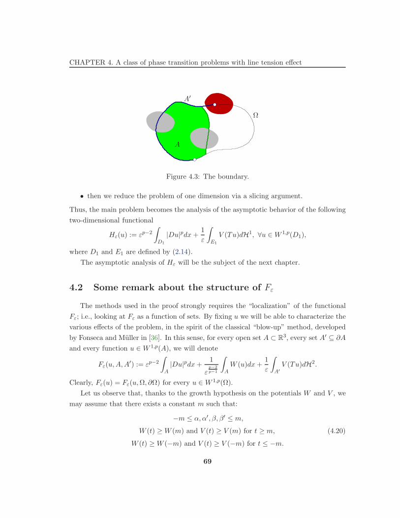
CHAPTER 4. A class of phase transition problems with line tension effect
A
A′
Ω
Figure 4.3: The boundary.
• then we reduce the problem of one dimension via a slicing argument.
Thus, the main problem becomes the analysis of the asymptotic behavior of the following
two-dimensional functional
Hε(u) := εp−2
∫
D1
|Du|pdx+1
ε
∫
E1
V (Tu)dH1, ∀u ∈W 1,p(D1),
where D1 and E1 are defined by (2.14).
The asymptotic analysis of Hε will be the subject of the next chapter.
4.2 Some remark about the structure of Fε
The methods used in the proof strongly requires the “localization” of the functional
Fε; i.e., looking at Fε as a function of sets. By fixing u we will be able to characterize the
various effects of the problem, in the spirit of the classical “blow-up” method, developed
by Fonseca and Muller in [36]. In this sense, for every open set A ⊂ R3, every set A′ ⊆ ∂A
and every function u ∈W 1,p(A), we will denote
Fε(u,A,A′) := εp−2
∫
A|Du|pdx+
1
εp−2p−1
∫
AW (u)dx+
1
ε
∫
A′
V (Tu)dH2.
Clearly, Fε(u) = Fε(u,Ω, ∂Ω) for every u ∈W 1,p(Ω).
Let us observe that, thanks to the growth hypothesis on the potentials W and V , we
may assume that there exists a constant m such that:
−m ≤ α,α′, β, β′ ≤ m,
W (t) ≥W (m) and V (t) ≥ V (m) for t ≥ m, (4.20)
W (t) ≥W (−m) and V (t) ≥ V (−m) for t ≤ −m.
69
CHAPTER 4. A class of phase transition problems with line tension effect
In particular, assumption (4.20) will allow us to use the truncation argument given by
the following Lemma.
Lemma 4.4. Let a domain A ⊂ R3, a set A′ ⊆ ∂A, and a sequence (uε) ⊂W 1,p(A) with
uniformly bounded energies Fε(uε, A,A′) be given. If we set uε(x) := (uε(x) ∧m) ∨−m),
then
(i) Fε(uε, A,A′) ≤ Fε(uε, A,A
′),
(ii) ‖uε − uε‖L1(A) and ‖T uε − Tuε‖L1(A′) vanish as ε→ 0.
Proof. The inequality Fε(uε, A,A′) ≤ Fε(uε, A,A
′) follows immediately from (4.20).
Statement (ii) follows from the fact that both W and V have growth at least linear at
infinity and the integrals
∫
W (uε)dx and
∫
V (Tuε)dx vanish as ε goes to 0.
Since W is strictly positive and continuous out of α and β, for every δ > 0, there exist
a > 0 and M > 0 such that
W (t) ≥ a ∀t ∈ [−M,α− δ] ∪ [β + δ,M ].
Moreover, since W has growth at least linear at infinity, we can find b > 0 such that
W (t) ≥ b|t| when |t| > M.
For every δ > 0, we define
Am := x ∈ A : m+ δ ≤ |uε(x)| ≤M and AM := x ∈ A : |uε(x)| ≥M .
We have
‖uε − uε‖L1(A) =
∫
A\(Am∩AM )|uε − uε|dx+
∫
Am
|uε − uε|dx+
∫
AM
|uε − uε|dx
≤ δ|A| +M |Am| +∫
AM
|uε|dx
(4.21)
≤ δ|A| + M
a
∫
Am
W (uε)dx+1
b
∫
AM
W (uε)dx
≤ δ|A| +(
M
a+
1
b
)∫
AW (uε)dx.
70
CHAPTER 4. A class of phase transition problems with line tension effect
Since the sequence (uε) has uniformly bounded energy, there exists a constant C such
that1
εp−2p−1
∫
AW (uε)dx ≤ C. (4.22)
Then, by (4.21) and (4.22), if follows
‖uε − uε‖L1(A) ≤ δ|A| + C
(
M
a+
1
b
)
εp−2p−1 . (4.23)
Passing to the limit as ε goes to 0 in (4.23), we obtain
lim supε→0
‖uε − uε‖L1(A) ≤ δ|A|.
The proof is complete by the arbitrariness of δ. 2
71
Chapter 5
Recovering the “contribution of
the wall”: the flat case
We will obtain “the contribution of the wall” to the limit energy Φ, defined by (4.2),
namely γpH1(Sv), by estimating the asymptotic behavior of the functional
Fε(u,B ∩ Ω, B ∩ ∂Ω) = εp−2
∫
B∩Ω|Du|pdx+
1
εp−2p−1
∫
B∩ΩW (u)dx+
∫
B∩∂ΩV (Tu)dH2,
when B is a small ball centered on ∂Ω and B ∩ ∂Ω is a flat disk. We will follow the idea
of Alberti, Bouchitte and Seppecher in [9], using a suitable slicing argument. Later on we
will show that the flatness assumption on B ∩ ∂Ω can be dropped when B is sufficiently
small. Hence, we need to prove a compactness result and a lower bound inequality for
the following two-dimensional functional
Hε(u) := εp−2
∫
D1
|Du|pdx+1
ε
∫
E1
V (Tu)dH1, ∀u ∈W 1,p(D1; [−m,m]), (5.1)
where Er and Dr are defined by (2.14). We recall that we will always study Hε like a
reduction of Fε. Hence there will be some hypotheses inherited by this reduction. In
particular, the hypothesis u ∈ [−m,m] in (5.1) is justified by Lemma 4.4.
Let us introduce the “localization” of the functional Hε. For every open set A ⊂ R2,
every set A′ ⊂ ∂A and every function u ∈W 1,p(A), we will denote
Hε(u,A,A′) := εp−2
∫
A|Du|pdx+
1
ε
∫
A′
V (Tu)dH1. (5.2)
If we set u(ε)(x) := u(εx) and A/ε := x : εx ∈ A, by scaling it is immediately seen
that
Hε(u,A,A′) = H1(u
(ε), A/ε,A′/ε). (5.3)
72

CHAPTER 5. Recovering the “contribution of the wall”: the flat case
In view of this scaling property, we consider the optimal profile problem, introduced in
the previous chapter; that is,
γp = inf
∫
R2+
|Du|pdx+
∫
R
V (Tu)dH1 : u ∈ L1loc(R
2+) :
∫
R2+
|Du|pdx is finite,
limt→−∞
Tu(t) = α′, limt→+∞
Tu(t) = β′
(5.4)
and determines the line tension on the limit energy Φ.
5.1 Compactness of the traces
We prove the pre-compactness of the traces of the sequences equi-bounded for Hε,
using the trace imbedding of W 1−1/p,p(∂D1) in W 1,p(D1) and Theorem 3.1(i); that is, the
compactness result for the one-dimensional functional Kε (see Section 3.3, p. 51).
Proposition 5.1. If (uε) ⊂W 1,p(D1; [−m,m]) is a sequence such that Hε(uε) is bounded,
then (Tuε) is pre-compact in L1(E1) and every cluster point belongs to BV (E1, α′, β′).
Proof. By hypothesis, there exists a constant C such that Hε(uε) ≤ C.
By the trace imbedding of W 1−1/p,p(∂D1) in W 1,p(D1), there exists a constant Cp
such that for every u ∈W 1,p(D1)
‖Tu‖W 1−1/p,p(∂D1) ≤ Cp‖u‖W 1,p(D1).
It follows that there exists a constant (still denoted by Cp) such that
∫ ∫
E1×E1
|Tuε(t) − Tuε(t′)|p
|t− t′|p dt′dt ≤ Cp
∫
D1
|uε|pdx+Cp
∫
D1
|Duε|pdx
(5.5)
≤ Cpπ
2mp + Cp
∫
D1
|Duε|pdx.
It follows that
Kε(Tuε, E1) ≤Cpπm
p
2εp−2 + (1 ∧ Cp)Hε(uε) ≤ C, (5.6)
where we used the equi-boundedness of uε. Hence, by (5.6), we have that the sequence
(Tuε) is equi-bounded for Kε and then we can use Theorem 3.1(i) to obtain the desired
conclusion. 2
73

CHAPTER 5. Recovering the “contribution of the wall”: the flat case
5.2 Lower bound inequality
Now, we will prove an optimal lower bound for Hε.
Proposition 5.2. For every (u, v) in BV (D1, α, β) × BV (E1, α′, β′) and every se-
quence (uε) ⊂W 1,p(D1; [−m,m]) such that uε → u in L1(D1) and Tuε → v in L1(E1)
lim infε→0
Hε(uε) ≥ γpH0(Sv). (5.7)
Proof. We will prove the lower bound inequality (5.7) for v such that
v(t) =
α′, if t ∈ (−1, 0],
β′, if t ∈ (0, 1).
Let us consider the natural extension of v to the whole real line R (still denoted by v);
i.e.,
v(t) =
α′, if t ≤ 0,
β′, if t > 0.
Step 0: Strategy of the proof. We are looking for an extension of uε to the whole R2+,
namely wε, such that wε is a competitor for (5.4) and Hε(wε,R2+,R) ≃ Hε(uε,D1, E1) as
ε→ 0 in a precise sense. More exactly, we will able to find s < 1 and we will construct a
competitor wε such that, for any given δ > 0 there exists εδ > 0 such that
Hε(uε) ≥ Hε(uε,Ds, Es)
= Hε(wε,R2+,R) −Hε(wε,R
2+ \Ds,R \ Es)
≥ γp − δ, ∀ε ≤ εδ.
Step 1: Construction of the competitor. For every s > 0, we define the harmonic extension
of v from R \ Es to R2+ \Ds, namely u, defined in polar coordinates by
u(ρ, θ) :=θ
πα′ +
(
1 − θ
π
)
β′, ∀θ ∈ [0, π), ∀ρ ≥ s.
We will construct the competitor wε simply gluing the function u and the function uε.
Hence, for every ε > 0, we consider the cut-off function ϕ in C∞(R2+), such that ϕ ≡ 1 in
74
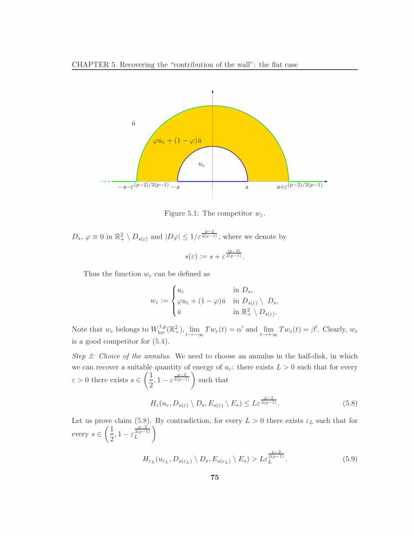
CHAPTER 5. Recovering the “contribution of the wall”: the flat case
−s−ε(p−2)/2(p−1) −s s s+ε(p−2)/2(p−1)
uǫ
u
ϕuε + (1 − ϕ)u
Figure 5.1: The competitor wε.
Ds, ϕ ≡ 0 in R2+ \Ds(ε) and |Dϕ| ≤ 1/ε
p−22(p−1) , where we denote by
s(ε) := s+ ε(p−2)2(p−1) .
Thus the function wε can be defined as
wε :=
uε in Ds,
ϕuε + (1 − ϕ)u in Ds(ε) \ Ds,
u in R2+ \Ds(ε).
Note that wε belongs to W 1,ploc (R2
+), limt→−∞
Twε(t) = α′ and limt→+∞
Twε(t) = β′. Clearly, wε
is a good competitor for (5.4).
Step 2: Choice of the annulus. We need to choose an annulus in the half-disk, in which
we can recover a suitable quantity of energy of uε: there exists L > 0 such that for every
ε > 0 there exists s ∈(
1
2, 1 − ε
p−22(p−1)
)
such that
Hε(uε,Ds(ε) \Ds, Es(ε) \ Es) ≤ Lεp−2
2(p−1) . (5.8)
Let us prove claim (5.8). By contradiction, for every L > 0 there exists εL such that for
every s ∈(
1
2, 1 − ε
p−22(p−1)
L
)
HεL(uεL
,Ds(εL) \Ds, Es(εL) \Es) > Lεp−2
2(p−1)
L . (5.9)
75
CHAPTER 5. Recovering the “contribution of the wall”: the flat case
In particular, we can choose a finite set (sk), for k = 1, 2, ...,
[
ε− p−2
2(p−1)
L
]
, such that
⋃
k
(Dsk(εL) \Dsk) = D1 \D1/2, (5.10)
with Dsk(εL) \Dskdisjoint sets.
By (5.9) and (5.10), we get
HεL(uεL
,D1, E1) ≥
"
ε−
p−22(p−1)
L
#
∑
k=1
HεL(uεL
,Dsk(εL) \Dsk, Esk(εL) \Esk
)
(5.11)
>
"
ε−
p−22(p−1)
L
#
∑
k=1
Lεp−2
2(p−1)
L = L
[
ε− p−2
2(p−1)
L
]
εp−2
2(p−1)
L ≥ L.
Since (uε) is equi-bounded, by taking the limit of L to +∞ in (5.11), we have a contra-
diction.
Step 3: Estimates. By the scaling property of Hε (see (5.3)), we have
γp ≤ H1(w(ε)ε ,R2
+,R) = Hε(wε,R2+/ε,R/ε)
≤ Hε(wε,R2+,R) = Hε(wε,Ds, Es) +Hε(wε,R
2+ \Ds,R \ Es)
(5.12)
≤ Hε(uε) + εp−2
∫
R2+\Ds
|Dwε|pdx+1
ε
∫
R\Es
V (Twε)dH1
= Hε(uε) + I1 + I2.
By definition of wε, the first integral in the right hand side of (5.12) can be easily estimated
as follows
I1 = εp−2
∫
R2+\Ds(ε)
|Du|pdx+ εp−2
∫
Ds(ε)\Ds
|D(ϕuε + (1 − ϕ)u)|pdx
≤ 3p−1εp−2
∫
R2+\Ds
|Du|pdx+ 3p−1εp−2
∫
Ds(ε)\Ds
|Duε|pdx
+6p−1mpπεp(p−2)2(p−1) + 3p−1(2m)pπsε
p−22 ,
76
CHAPTER 5. Recovering the “contribution of the wall”: the flat case
where we used the fact that∫
Ds(ε)\Ds
|Dϕ|p|uε − u|pdx ≤ 1
εp(p−2)2(p−1)
∫
Ds(ε)\Ds
|uε − u|p
≤ 2p−1mpπ
(
1
ε(p−2)2
2(p−1)
+2s
εp−22
)
and that |uε| < m and |u| < m.
By definition of u, we have∫
R2+\Ds
|Du|pdx =|β′ − α′|p
πp−1(p− 2)sp−2.
Hence,
I1 ≤ 3p−1εp−2
∫
Ds(ε)\Ds
|Duε|pdx+3p−1|β′ − α′|p
(p− 2)πp−2sp−2εp−2
+6p−1mpπεp(p−2)2(p−1) + 3p−1(2m)pπsε
p−22 . (5.13)
Let us estimate the second integral in the right hand side of (5.12). Since Twε = α′
and Twε = β′ on R \ Es(ε), we have
I2 =1
ε
∫
R\Es(ε)
V (T u)dH1 +1
ε
∫
Es(ε)\Es
V (Twε)dH1 ≡ 1
ε
∫
Es(ε)\Es
V (Twε)dH1.
For every δ > 0, let us define
Eδ :=
x ∈ Es(ε) \ Es : |Tuε − β′| > δ and |Tuε − α′| > δ
.
Thanks to Step 2, we get: there exists N >L
ωδ(where we denote by ωδ := min
|t−α′|≥δ
|t−β′|≥δ
V (t))
such that for every δ > 0 there exists εδ such that
|Eδ | ≤ Nεp−2
2(p−1) ε, ∀ε ≤ εδ, (5.14)
In particular, choosing δ small, the convexity of V near its wells provides
I2 =1
ε
∫
(Es(ε)\Es)\Eδ
V (Twε)dH1 +1
ε
∫
Eδ
V (Twε)dH1
(5.15)
≤ 1
ε
∫
(Es(ε)\Es)\Eδ
V (Tuε)dH1 + ωmNεp−2
2(p−1) ,
77
CHAPTER 5. Recovering the “contribution of the wall”: the flat case
where ωm := max|t|<m
V (t) and we used the inequality (5.14).
Finally, by (5.12), (5.13) and (5.15), we obtain, for every δ > 0
Hε(uε) ≥ γp −(
3p−1Hε(wε,Ds(ε) \Ds, Es(ε) \ Es) +3p−1|β′ − α′|p
(p− 2)πp−1sp−2εp−2
6p−1mpπεp(p−2)2(p−1) + 3p−1(2m)pπsε
p−22 + ωmNε
p−22(p−1)
)
,
(5.16)
≥ γp −(
3p−1Lε+3p−1|β′ − α′|p
(p− 2)πp−1sp−2εp−2
6p−1mpπεp(p−2)2(p−1) + 3p−1(2m)pπsε
p−22 + ωmNε
p−22(p−1)
)
, ∀ε ≤ εδ.
Notice that for every ε > 0, s ∈(
1/2, 1 − εp−2
2(p−1)
)
. Hence, taking the limit as ε → 0,
we get lim infε→0
Hε(uε) ≥ γp, which concludes the proof. 2
5.3 Reduction to the flat case
We prove compactness and a lower bound inequality for the following energies
Fε(uε,D,E) = εp−2
∫
D|Du|pdx+
1
εp−2p−1
∫
DW (u)dx+
1
ε
∫
EV (Tu)dH2,
where D ⊂ R3 is the open half-ball centered in 0 with radius r > 0 and E ⊂ R
2 is its
“diameter”; that is,
E :=
(x1, x2, x3) ∈ R2 : |x| ≤ r, x3 = 0
.
We will reduce to Proposition 5.1 and Proposition 5.2 via a suitable slicing argument. In
the following we use the notation introduced in Section 1.3: e is an unit vector in the
plane P := x3 = 0; M is the orthogonal complement of e in P ; π is the projection of
R3 onto M ; for every y ∈ Ee := π(E), we denote by Ey := π−1(y)∩E, Dy := π−1(y)∩D
(see Fig. 5.2).
Proposition 5.3. Let (uε) ⊂ W 1,p(D; [−m,m]) be a sequence with uniformly bounded
energies Fε(uε,D,E). Then the traces Tuε are pre-compact in L1(E) and every cluster
78
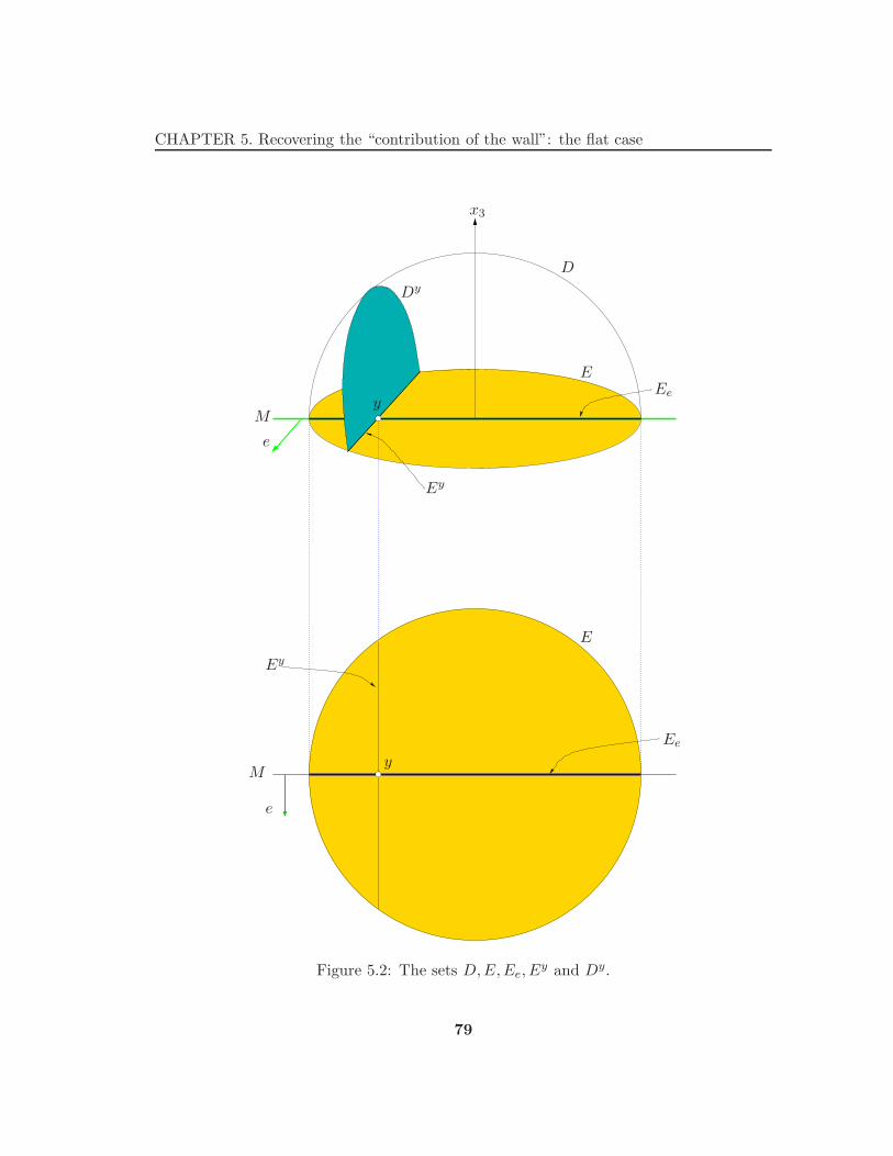
CHAPTER 5. Recovering the “contribution of the wall”: the flat case
D
E
E
Dy
y
y
x3
Ee
Ee
Ey
Ey
M
M
e
e
Figure 5.2: The sets D,E,Ee, Ey and Dy.
79
CHAPTER 5. Recovering the “contribution of the wall”: the flat case
point belongs to BV (E, α′, β′). Moreover, if Tuε → v in L1(E), then
lim infε→0
Fε(uε,D,E) ≥ γp
∣
∣
∣
∣
∫
E∩Svνv
∣
∣
∣
∣
dH1. (5.17)
Proof. By Fubini’s Theorem, for every ε > 0, we get
Fε(uε,D,E) ≥ εp−2
∫
D|Duε|pdx+
1
ε
∫
EV (Tuε)dH2
≥∫
Ee
[
εp−2
∫
Dy
|Duyε |pdx+1
ε
∫
Ey
V (Tuyε)dH1
]
dy
(5.18)
=
∫
Ee
Hε(uyε ,D
y, Ey)dy
We first prove that (Tuε) is pre-compact in L1(E). In view of Theorem 1.9, it suffices
to show that the family F := (Tuε) satisfies the following property: for every δ > 0
there exists a family Fδ δ-dense in F such that (Fδ)ye is pre-compact in L1(E) for H2-a.e.
y ∈ Ee. By assumption Fε(uε,D,E) ≤ C, by (5.18) we have
∫
Ee
Hε(uyε ,D
y, Ey)dy ≤ C. (5.19)
Fix δ > 0 and, for every ε > 0, define vε : E → [−m,m] such that
vyε :=
Tuyε if y ∈ Ee and Hε(uyε ,Dy, Ey) ≤ 2mrC/δ,
α′ otherwise.(5.20)
By (5.19), we have vyε = Tuyε for every y ∈ Ee apart from a subset of measure smaller
than δ/2mr. Hence, vε = Tuε in E up to a set of measure smaller than δ/m. So, from
|Tuε| ≤ m, we deduce
‖vε − Tuε‖L1(E) ≤ δ.
Therefore, the family Fδ := (vε) is δ−dense in F .
By (5.20), Hε(vyε ,D
y, Ey) ≤ 2mrC/δ for every y ∈ Ee and this implies that the
sequence (vyε ) is pre-compact in L1(Ey). By Theorem 1.9(i), the sequence (Tuε) is pre-
compact in L1(E); i.e., there exists a function v ∈ L1(E) such that
Tuε → v in L1(E).
80
CHAPTER 5. Recovering the “contribution of the wall”: the flat case
Let us show that v belongs to BV (E, α′, β′). We have that (up to a subsequence)
Tuyε → vy in L1(E) for a.e. y ∈ Ee.
Then, by Proposition 5.1, we have that vy ∈ BV (Ey, α′, β′). Hence, by slicing property
for BV functions, it follows that v ∈ BV (E, α′, β′) (see [32], Section 5.10, for details).
It remains to prove that inequality (5.17) holds. Taking the limit as ε → 0 in (5.18),
by Fatou’s Lemma, we deduce that
lim infε→0
Fε(uε,D,E) ≥∫
Ee
lim infε→0
Hε(uyε ,D
y, Ey)dy.
Then, using the Proposition 5.2, we get
lim infε→0
Fε(uε,D,E) ≥∫
Ee
γpH0(Svy)dy. (5.21)
The right-hand side of (5.21) is finite and Svy agrees with Sv ∩ Ey for a.e. y ∈ Ee. By
(1.5)1 we may rewrite (5.21) as
lim infε→0
Fε(uε,D,E) ≥ γp
∫
E∩Sv〈νv, e〉dH1. (5.22)
Finally, (5.17) follows from (5.22) by choosing a suitable unit vector e. 2
5.4 Existence of an optimal profile problem
We conclude this chapter with the proof of the existence of a minimum for the optimal
profile problem (5.4). We will use a rearrangement result in one direction to show that
the minimum for γp is achieved by a function with non-decreasing trace.
Proposition 5.4. The minimum for γp defined by (5.4) is achieved by a function u such
that Tu is a non-decreasing function in R.
Proof. Note that, since the energy H1 is decreasing under truncation by α′ and β′, it is
not restrictive to minimize the problem (5.4) with the additional condition α′ ≤ u ≤ β′.
1See Proposition 1.7, p. 26.
81
CHAPTER 5. Recovering the “contribution of the wall”: the flat case
We denote by X the class of all w : R → [α′, β′] such that w ∈ L1loc(R
2+),
∫
R2+
|Dw|pdx
is finite, limt→−∞
Tw(t) = α′, limt→+∞
Tw(t) = β′; we denote by X∗ the class of all w ∈ X such
that Tw is non-decreasing, Tw(t) ≥ α′ + β′
2for t > 0 and Tw(t) ≤ α′ + β′
2for t < 0.
Step 1: The infimum of H1 on X is equal to the infimum of H1 on X∗.
Since X∗ ⊂ X we have
infw∈X∗
H1(w,R2+,R) ≥ inf
w∈XH1(w,R
2+,R). (5.23)
Fix u in X, we claim that for every δ > 0 there exists a function uδ in X∗ such that
H1(uδ ,R2+,R) ≤ H1(u,R
2+,R) + o(δ). (5.24)
Once we have (5.24), for every δ > 0, we get
infw∈X∗
H1(w,R2+,R) ≤ H1(u,R
2+,R) + o(δ), ∀u ∈ X.
Taking the limit for δ → 0 and then the infimum on u ∈ X, we obtain
infw∈X∗
H1(w,R2+,R) ≤ inf
u∈XH1(u,R
2+,R)
and this together with (5.23) conclude the proof of the step. It remain to prove (5.24).
For every S > 0, we denote by
QS := [−S, S] × [0, S]
and by u⋆ the monotone increasing rearrangement in x1 of u in QS (see Section 1.4.2, p.
31).
For every R > 0, we define the harmonic extension of the function
α′χ(−∞,0)(t) + β′(1 − χ[0,+∞)(t))
from R \ER to R2+ \DR; i.e., the function u that expressed in polar coordinates is given
by
u(ρ, θ) :=θ
πα′ +
(
1 − θ
π
)
β′, ∀θ ∈ [0, π], ∀ρ ≥ R.
We will construct a function u ∈ X∗ gluing the function u and the function u⋆. Hence,
for every S ≥ R > 0, we consider the cut-off function ϕ such that
ϕ = 0 in DR, ϕ = 1 in R2+ \DS and |Dϕ| ≤ 1/(S −R) in DS \DR.
82
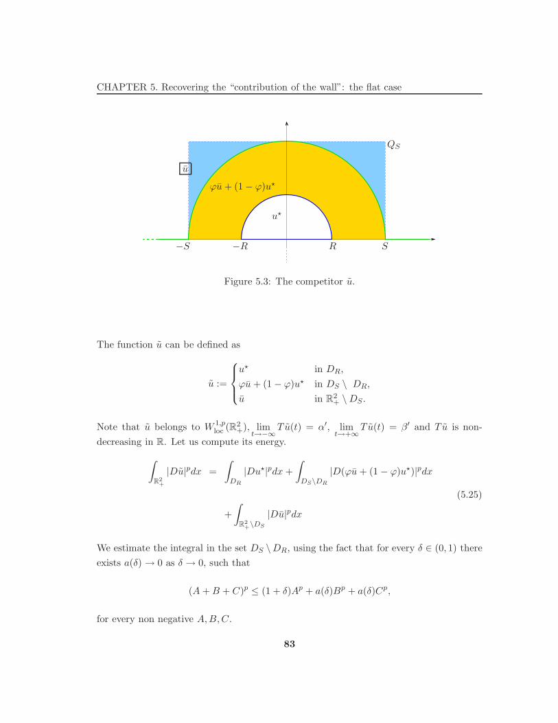
CHAPTER 5. Recovering the “contribution of the wall”: the flat case
u
ϕu+ (1 − ϕ)u⋆
u⋆
−S −R R S
QS
Figure 5.3: The competitor u.
The function u can be defined as
u :=
u⋆ in DR,
ϕu+ (1 − ϕ)u⋆ in DS \ DR,
u in R2+ \DS .
Note that u belongs to W 1,ploc (R2
+), limt→−∞
T u(t) = α′, limt→+∞
T u(t) = β′ and T u is non-
decreasing in R. Let us compute its energy.
∫
R2+
|Du|pdx =
∫
DR
|Du⋆|pdx+
∫
DS\DR
|D(ϕu+ (1 − ϕ)u⋆)|pdx
(5.25)
+
∫
R2+\DS
|Du|pdx
We estimate the integral in the set DS \DR, using the fact that for every δ ∈ (0, 1) there
exists a(δ) → 0 as δ → 0, such that
(A+B + C)p ≤ (1 + δ)Ap + a(δ)Bp + a(δ)Cp,
for every non negative A,B,C.
83

CHAPTER 5. Recovering the “contribution of the wall”: the flat case
Hence, for every δ ∈ (0, 1), we have
∫
DS\DR
|D(ϕu+ (1 − ϕ)u⋆)|pdx ≤ (1 + δ)
∫
DS\DR
|Du⋆|pdx+ a(δ)
∫
DS\DR
|Du|pdx
(5.26)
+a(δ)|β′ − α′|pπ2(S2 −R2)
(S −R)p,
where we used that |Dϕ| ≤ 1/(S−R) and u, u⋆ ∈ [α′, β′]. By (5.25) and (5.26), we obtain
∫
R2+
|Du|pdx ≤ (1 + δ)
∫
DS
|Du⋆|pdx+ a(δ)
∫
R2+\DR
|Du|pdx
(5.27)
+a(δ)|β′ − α′|pπ2(S2 −R2)
(S −R)p.
We can estimates the first term in the right hand side of (5.27) using the fact that
monotone increasing rearrangement in one direction decreases the Lp-norm of the gradient
(see Theorem 1.16, p. 31).
∫
DS
|Du⋆|pdx ≤∫
QS
|Du⋆|pdx ≤∫
QS
|Du|pdx. (5.28)
The second term in the right hand side of (5.27) can be explicitly computed
∫
R2+\DR
|Du|pdx =πp−1|β′ − α′|p(p− 2)Rp−2
. (5.29)
Finally, putting together (5.27), (5.28) and (5.29), we obtain that, for every S ≥ R > 0
and every δ ∈ (0, 1), the following estimate holds
∫
R2+
|Du|pdx ≤ (1 + δ)
∫
R2+
|Du|pdx+a(δ)πp−1|β′ − α′|p
(p − 2)Rp−2
(5.30)
+a(δ)|β′ − α′|pπ2(S2 −R2)
(S −R)p,
with a(δ) → +∞ as δ → 0. In particular,
∫
R2+
|Du|pdx is finite.
84
CHAPTER 5. Recovering the “contribution of the wall”: the flat case
Now, we evaluate the second term of H1(u,R2+,R).
∫
R
V (T u)dH1 =
∫
ES\ER
V(
ϕu+ (1 − ϕ)Tu⋆)
dH1
(5.31)
+
∫
ER
V (Tu⋆)dH1,
where we used that, by definition, u(t) = α′ if t < −S and u(t) = β′ if t > S.
Since Tu(t) tends to α′ and β′ as t → −∞ and +∞ respectively and V is convex
near the wells, there exists R0 > 0 such that Tu(t) lies in the convex wells of V for all
t ∈ R \ ER, for every R > R0, and the same does Tu⋆(t). This implies that for any
S > R > R0 we have
∫
ES\ER
V(
ϕu+ (1 − ϕ)Tu⋆)
dH1 ≤∫
ES\ER
ϕV (u)dH1 +
∫
ES\ER
(1 − ϕ)V (Tu⋆)dH1
≤∫
ES\ER
V (Tu⋆)dH1. (5.32)
By (5.31) and (5.32), we have
∫
R
V (T u)dH1 ≤∫
ES
V (Tu⋆)dH1 =
∫
ES
V (Tu)dH1
(5.33)
≤∫
R
V (Tu)dH1.
Finally, by (5.30) and (5.33), we have the following estimate, for every S ≥ R > R0 > 0
and every δ ∈ (0, 1)
H1(u,R2+,R) ≤ (1 + δ)H1(u) +
a(δ)πp−1|β′ − α′|p(p− 2)Rp−2
(5.34)
+a(δ)|β′ − α′|pπ2(S2 −R2)
(S −R)p.
This proves the claim, taking R and S −R large enough.
Step 2: The infimum of H1 on X∗ is achieved.
We use the Direct Method. Take a minimizing sequence (un) ⊂ X∗. In particular,
85
CHAPTER 5. Recovering the “contribution of the wall”: the flat case
H1(un,R2+,R) ≤ C, Dun converges weakly to Du in Lp(R2
+) and un converges to u weakly
in W 1,ploc (R2
+). Since
∫
R2+
|Dun|pdx is bounded, we can find a function u ∈ L1loc(R
2+) and
∫
R2+
|Du|pdx is finite, such that (up to a subsequence)
Dun Du in Lp(R2+) and un u in Lploc(R
2+).
By the trace imbedding of W 1−1/p,p in W 1,p, we have
Tun Tu in W1−1/p,ploc (R).
By the compact embedding of W1−1/p,ploc (R) in C0
loc(R) (see [1], Theorem 7.34, p. 231),
we have that, up to a subsequence, Tun uniformly converges to Tu. Thus Tu is non-
decreasing and satisfies
Tu(t) ≥ α′ + β′
2for t > 0 and Tu(t) ≤ α′ + β′
2for t < 0.
Let us show that limt→−∞
Tu(t) = α′ and limt→+∞
Tu(t) = β′. Since Tu is non-decreasing in
[α′, β′], there exist a ≤ α′ + β′
2and b ≥ α′ + β′
2such that
a := limt→−∞
Tu(t) and b := limt→+∞
Tu(t).
By contradiction, we assume that either a 6= α′ or b 6= β′. Then, since V is continuous
and strictly positive in (α′, β′), we obtain
∫
R
V (Tu)dH1 = +∞,
This is impossible, because, by Fatou’s Lemma, we have
∫
R
V (Tu)dH1 ≤ lim infn→+∞
∫
R
V (Tun)dH1 < lim infn→+∞
H1(un,R2+,R) < +∞.
Hence, u is in X∗. Since H1 is clearly lower semicontinuous on sequences such that
Dun Du in Lp and Tun → Tu pointwise, this concludes the proof. 2
86

Chapter 6
Proof of the main result
In this chapter, we will prove the main result of this thesis, namely the compactness, the
lower bound inequality and the upper bound inequality stated in Theorem 4.1.
For the sake of simplicity, we recall the definition of the functionals which we deal
with:
Fε(u) = εp−2
∫
Ω|Du|pdx+
1
εp−2p−1
∫
ΩW (u)dx+
1
ε
∫
∂ΩV (Tu)dH2, ∀u ∈W 1,p(Ω), (6.1)
and
Φ(u, v) = σpH2(Su) + cp
∫
∂Ω|W(Tu) −W(v)|dH2 + γpH1(Sv),
∀(u, v) ∈ BV (Ω, α, β) ×BV (∂Ω, α′, β′). (6.2)
Theorem 6.1. Let Fε : W 1,p(Ω) → R and Φ : BV (Ω, α, β) × BV (∂Ω, α′, β′) → R
defined by (6.1) and (6.2).
Then
(i) [Compactness] If (uε) ⊂ W 1,p(Ω) is a sequence such that Fε(uε) is bounded,
then (uε, Tuε) is pre-compact in L1(Ω) × L1(∂Ω) and every cluster point belongs
to BV (Ω, α, β) ×BV (∂Ω, α′, β′).
(ii) [Lower Bound Inequality] For every (u, v) ∈ BV (Ω, α, β)×BV (∂Ω, α′, β′)and every sequence (uε) ⊂ W 1,p(Ω) such that uε → u in L1(Ω) and Tuε → v in
L1(∂Ω),
lim infε→0
Fε(uε) ≥ Φ(u, v).
87
CHAPTER 6. Proof of the main result
(iii) [Upper Bound Inequality] For every (u, v) ∈ BV (Ω, α, β)×BV (∂Ω, α′, β′)there exists a sequence (uε) ⊂ W 1,p(Ω) such that uε → u in L1(Ω), Tuε → v in
L1(∂Ω) and
lim supε→0
Fε(uε) ≤ Φ(u, v).
6.1 Compactness
Let a sequence (uε) ⊂ W 1,p(Ω) be given such that Fε(uε) is bounded. Since Fε(uε) ≥Fε(uε,Ω, ∅) ≡ Gε(uε,Ω), by the statement (i) of Theorem 2.2, the sequence (uε) is pre-
compact in L1(Ω) and there exists u ∈ BV (Ω, α, β) such that uε → u in L1(Ω).
It remains to prove that (Tuε) is pre-compact in L1(∂Ω) and that its cluster points are
in BV (∂Ω, α′, β′). Thanks to Proposition 1.12 we can cover ∂Ω with finitely many balls
(Bi)i∈I centered on ∂Ω, of radius ri such that for every i ∈ I there exists a bi-Lipschitz
map Ψi, with isometry defect δ(Ψi) < 1, which satisfies Ψi(Dri ∩ Bi) = Ω ∩ Bi and
Ψi(Eri ∩ Bi) = ∂Ω ∩ Bri (see Section 1.3.2, p. 29). We show that (Tuε) is pre-compact
in L1(∂Ω ∩Bi) for every i ∈ I.
For every fixed i, let us set
uiε := uε Ψi.
Since the isometry defect of Ψi is smaller than 1, Proposition 1.11 implies
Fε(uε,Ω ∩Bi, ∂Ω ∩Bi) ≥ (1 − δ(Ψi))p+3Fε(u
iε,Dri ∩Bi, Eri ∩Bi),
so Fε(uiε,Dri ∩ Bi, Eri ∩ Bi) is bounded. Hence, the compactness of the traces Tuiε in
L1(Eri) follows from Proposition 5.3. Finally, using the invertibility of Ψi, we have that
(Tuε) is pre-compact in L1(∂Ω) and that its cluster points are in BV (∂Ω, α′, β′). 2
6.2 Lower bound inequality
The proof of the lower bound inequality of Theorem 6.1 follows the lines of the proof
of Theorem 2.6(ii) by Alberti, Bouchitte and Seppecher in [9], but for the estimate of
the boundary effect we will use the optimal profile problem (5.4) in connection with the
results proved in the previous chapter.
88
CHAPTER 6. Proof of the main result
Let a sequence (uε) ⊂ W 1,p(Ω) be given such that uε → u ∈ BV (Ω, α, β) in L1(Ω)
and Tuε → v ∈ BV (∂Ω, α′β′) in L1(∂Ω). We have to prove that
lim infε→0
Fε(uε) ≥ Φ(u, v), (6.3)
where Φ is given by (6.2).
Clearly, we can assume that lim infε→0
Fε(uε) < +∞.
For every ε > 0, let µε be the energy distribution associated to Fε with configuration
uε; i.e., µε is the positive measure given by
µε(B) := εp−2
∫
Ω∩B|Duε|pdx+
1
εp−2p−1
∫
Ω∩BW (uε)dx+
1
ε
∫
∂Ω∩BV (Tuε)dH2, (6.4)
for every B ⊂ R3 Borel set.
Similarly, let us define
µ1(B) := σpH2(Su ∩B),
µ2(B) := cp
∫
∂Ω∩B|W(Tu) −W(v)|dH2,
µ3(B) := γpH1(Sv ∩B).
The total variation ‖µε‖ of the measure µε is equal to Fε(uε), and ‖µ1‖ + ‖µ3‖ + ‖µ3‖ is
equal to Φ(u, v). ‖µε‖ is bounded and we can assume that µε converges in the sense of
measure to some finite measure µ in R3. Then, by the lower semicontinuity of the total
variation, we have
lim infε→0
Fε(uε) ≡ lim infε→0
‖µε‖ ≥ ‖µ‖.
Since the measures µi are mutually singular, we obtain the lower bound inequality (6.3)
if we prove that
µ ≥ µi, for i = 1, 2, 3. (6.5)
We prove that µ ≥ µi by showing that µ(B) ≥ µi(B) for all sets B ⊂ R3 such that
B ∩ Ω is a Lipschitz domain and µ(∂B) = 0. This class is large enough to imply the
inequality (6.5) for all Borel sets B.
We have
µ(B) = limε→0
µε(B) ≥ lim infε→0
Fε(uε,Ω ∩B, ∅) ≥ σpH2(Su ∩B) ≡ µ1(B),
where the last inequality follows from statement (ii) of Theorem 2.2.
89
CHAPTER 6. Proof of the main result
Similarly, we can prove that µ ≥ µ2. We have
µ(B) = limε→0
µε(B) ≥ lim infε→0
Fε(uε,Ω ∩B, ∅) ≥ cp
∫
∂Ω∩B|W(Tu) −W(v)|dH2 ≡ µ2(B),
where we used Proposition 4.3(i) with A := B ∩ Ω and A′ := B ∩ ∂Ω.
The inequality µ ≥ µ3 requires a different argument. Notice that µ3 is the restriction
of H1 to the set Sv, multiplied by the factor γp. Thus, if we prove that
lim infr→0
µ(Br(x))
2r≥ γp, H1-a.e. x ∈ Sv, (6.6)
we obtain the required inequality. In fact, the left-hand side of (6.6) represents the
“one-dimensional density of the measure µ at x”, and it agrees with the Radon-Nykodim
derivative of the measure µ with respect to H1 Sv for H1-a.e. x ∈ Sv.
Let us fix x ∈ Sv such that there exists limr→0
µ(Br(x))
2rand Sv has one-dimensional
density equal to 1. We denote by νv the unit normal at x.
For r small enough, we choose a map Ψr such as in Proposition 1.12. Thus we have
Ψr(Dr) = Ω ∩Br(x), Ψr(Er) = ∂Ω ∩Br(x) and δ(Ψr) → 0 as r → 0.
Let us set
uε := uε Ψr and v := v Ψr.
Hence, T uε → v in L1(Er) and v ∈ BV (Er, α′, β′). So, thanks to Proposition 1.11, we
obtain
µ(Br(x)) = limε→0
µε(Br(x))
= limε→0
Fε(uε,Ω ∩Br(x), ∂Ω ∩Br(x)) (6.7)
≥ lim infε→0
(1 − δ(Ψr))p+3Fε(uε,Dr, Er).
Moreover, by Proposition 5.3, we have
lim infε→0
Fε(uε,Dr, Er) ≥ γp
∣
∣
∣
∣
∫
Sv∩Er
νvdH1
∣
∣
∣
∣
(6.8)
Finally, we notice that δ(Ψr) vanishes and
∣
∣
∣
∣
∫
Sv∩Er
νvdH1
∣
∣
∣
∣
= 2r + o(r) as r goes to 0. So
(6.7) and (6.8) give the following inequality
µ(Br(x))
2r≥ γp
(
1 +o(r)
2r
)
as r → 0,
90
CHAPTER 6. Proof of the main result
that implies µ ≥ µ3. This concludes the proof of the lower bound inequality. 2
6.3 Upper bound inequality
We will construct an optimal sequence uε according to Theorem 6.1(iii) in a suitable
partition of Ω. To this aim, and in order to use the preliminary convergence results stated
in the previous chapters, we need the following lemma
Lemma 6.2. Let A be a domain in R3, A′ ⊂ ∂A, v : A′ → [−m,m] a Lipschitz function
(where m is given by (4.20)) and Gε defined by (4.4).
Then, for every ε > 0, there exists an extension u : A→ [−m,m] such that
Lip(u) ≤ ε−p−2p−1 + Lip(v)
and
Gε(u,A) ≤(
(εp−2p−1 Lip(v) + 1)p + Cm
)
(
H2(∂A) + o(1))
ω, as ε→ 0, (6.9)
where Cm := maxt∈[−m,m]
W (t), ω := ‖v − α‖∞ ∧ ‖v − β‖∞.
Proof. It is not restrictive to assume that A′ = ∂A; in fact, we can extend v to ∂A
without increasing its Lipschitz constant (defining v(x) := infx′∈A′
v(x′) + Lip(v)|x − y| for
every x in ∂A). We additionally suppose that ω = ‖v − α‖∞ (the case ω = ‖v − β‖∞being similar).
Let us set
u(x) :=
v(x) on ∂A,
α on A \ Aωε(p−2)/(p−1) ,
where At is the set of all x in A such that 0 < dist(x, ∂A) < t.
Then, u is(
ε− p−2
p−1 + Lip(v))
-Lipschitz continuous on A \ Aωε(p−2)/(p−1) . Finally u can be
extended to A, without increasing its Lipschitz constant.
We have
Gε(u,A) = εp−2
∫
Aωε(p−2)/(p−1)
|Du|pdx+1
εp−1p−2
∫
Aωε(p−2)/(p−1)
W (u)dx
≤ |Aωε(p−2)/(p−1) |(
εp−2(Lip(v) +1
ε(p−1)/(p−2))p +
1
ε(p−1)/(p−2)Cm
)
=(
(H2(∂A) + o(1))(εp−1p−2 Lip(v) + 1)p + Cm
)
ω, as ε→ 0,
91
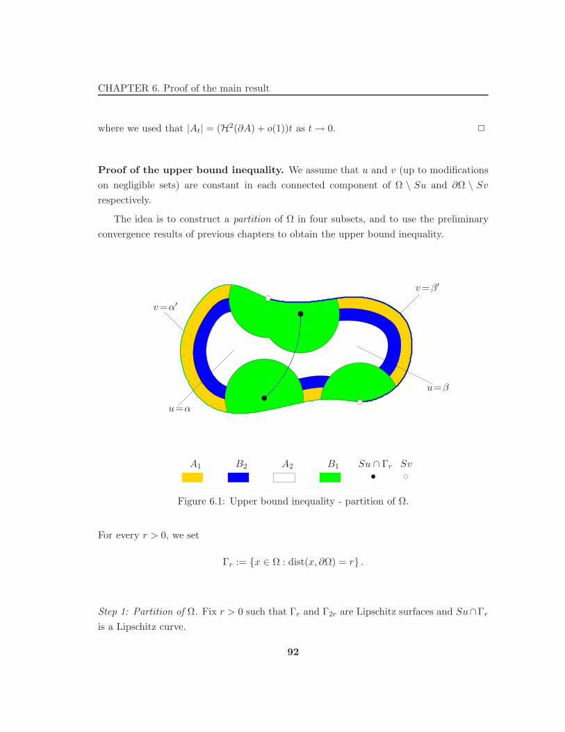
CHAPTER 6. Proof of the main result
where we used that |At| = (H2(∂A) + o(1))t as t→ 0. 2
Proof of the upper bound inequality. We assume that u and v (up to modifications
on negligible sets) are constant in each connected component of Ω \ Su and ∂Ω \ Svrespectively.
The idea is to construct a partition of Ω in four subsets, and to use the preliminary
convergence results of previous chapters to obtain the upper bound inequality.
u=α
u=β
v=α′
v=β′
A1 A2 B1B2 Su ∩ Γr Sv
Figure 6.1: Upper bound inequality - partition of Ω.
For every r > 0, we set
Γr := x ∈ Ω : dist(x, ∂Ω) = r .
Step 1: Partition of Ω. Fix r > 0 such that Γr and Γ2r are Lipschitz surfaces and Su∩Γr
is a Lipschitz curve.
92
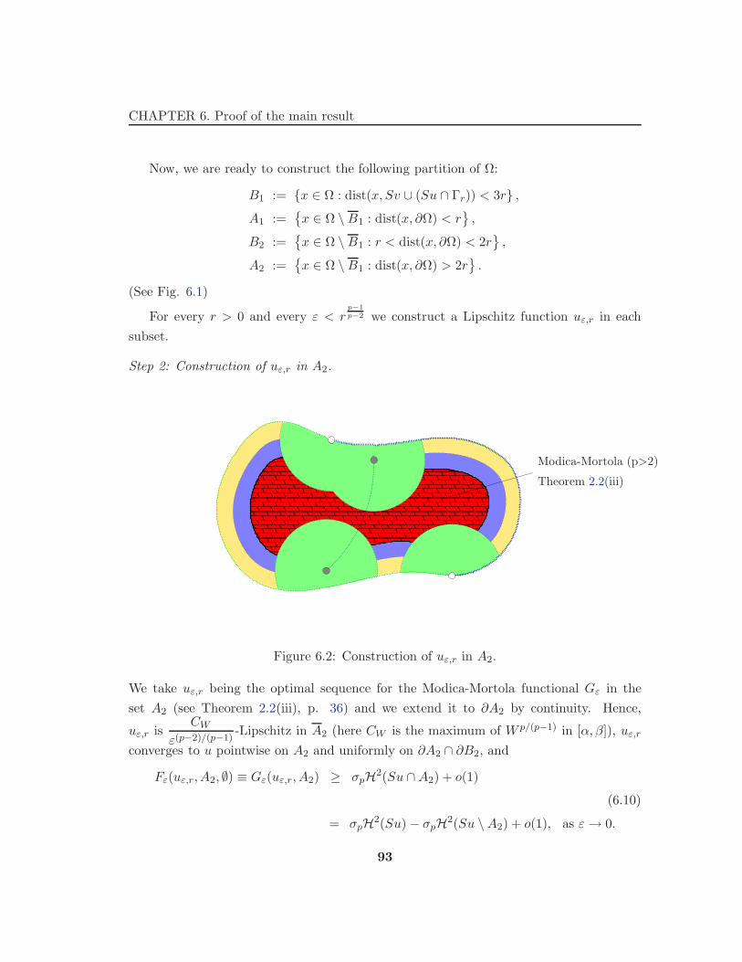
CHAPTER 6. Proof of the main result
Now, we are ready to construct the following partition of Ω:
B1 := x ∈ Ω : dist(x, Sv ∪ (Su ∩ Γr)) < 3r ,A1 :=
x ∈ Ω \B1 : dist(x, ∂Ω) < r
,
B2 :=
x ∈ Ω \B1 : r < dist(x, ∂Ω) < 2r
,
A2 :=
x ∈ Ω \B1 : dist(x, ∂Ω) > 2r
.
(See Fig. 6.1)
For every r > 0 and every ε < rp−1p−2 we construct a Lipschitz function uε,r in each
subset.
Step 2: Construction of uε,r in A2.
Modica-Mortola (p>2)
Theorem 2.2(iii)
Figure 6.2: Construction of uε,r in A2.
We take uε,r being the optimal sequence for the Modica-Mortola functional Gε in the
set A2 (see Theorem 2.2(iii), p. 36) and we extend it to ∂A2 by continuity. Hence,
uε,r isCW
ε(p−2)/(p−1)-Lipschitz in A2 (here CW is the maximum of W p/(p−1) in [α, β]), uε,r
converges to u pointwise on A2 and uniformly on ∂A2 ∩ ∂B2, and
Fε(uε,r, A2, ∅) ≡ Gε(uε,r, A2) ≥ σpH2(Su ∩A2) + o(1)
(6.10)
= σpH2(Su) − σpH2(Su \A2) + o(1), as ε→ 0.
93
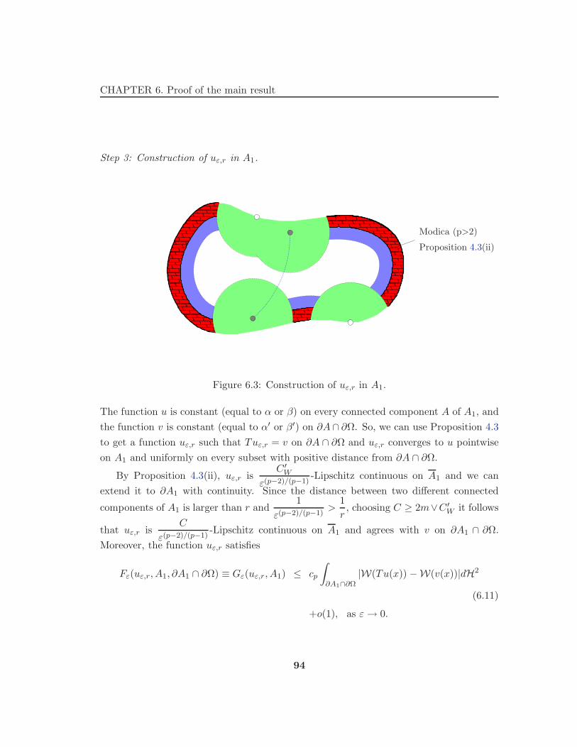
CHAPTER 6. Proof of the main result
Step 3: Construction of uε,r in A1.
Modica (p>2)
Proposition 4.3(ii)
Figure 6.3: Construction of uε,r in A1.
The function u is constant (equal to α or β) on every connected component A of A1, and
the function v is constant (equal to α′ or β′) on ∂A∩ ∂Ω. So, we can use Proposition 4.3
to get a function uε,r such that Tuε,r = v on ∂A ∩ ∂Ω and uε,r converges to u pointwise
on A1 and uniformly on every subset with positive distance from ∂A ∩ ∂Ω.
By Proposition 4.3(ii), uε,r isC ′W
ε(p−2)/(p−1)-Lipschitz continuous on A1 and we can
extend it to ∂A1 with continuity. Since the distance between two different connected
components of A1 is larger than r and1
ε(p−2)/(p−1)>
1
r, choosing C ≥ 2m∨C ′
W it follows
that uε,r isC
ε(p−2)/(p−1)-Lipschitz continuous on A1 and agrees with v on ∂A1 ∩ ∂Ω.
Moreover, the function uε,r satisfies
Fε(uε,r, A1, ∂A1 ∩ ∂Ω) ≡ Gε(uε,r, A1) ≤ cp
∫
∂A1∩∂Ω|W(Tu(x)) −W(v(x))|dH2
(6.11)
+o(1), as ε→ 0.
94
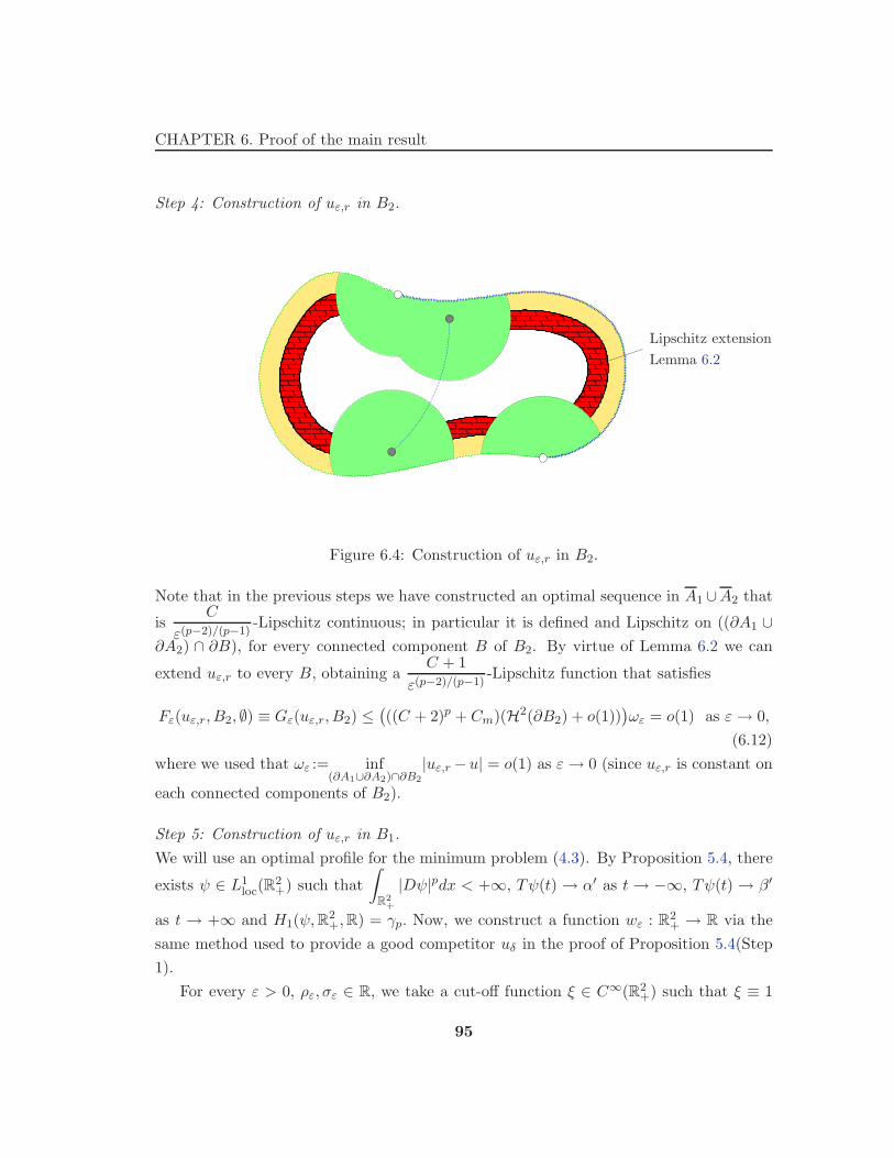
CHAPTER 6. Proof of the main result
Step 4: Construction of uε,r in B2.
Lipschitz extension
Lemma 6.2
Figure 6.4: Construction of uε,r in B2.
Note that in the previous steps we have constructed an optimal sequence in A1 ∪A2 that
isC
ε(p−2)/(p−1)-Lipschitz continuous; in particular it is defined and Lipschitz on ((∂A1 ∪
∂A2) ∩ ∂B), for every connected component B of B2. By virtue of Lemma 6.2 we can
extend uε,r to every B, obtaining aC + 1
ε(p−2)/(p−1)-Lipschitz function that satisfies
Fε(uε,r, B2, ∅) ≡ Gε(uε,r, B2) ≤(
((C + 2)p + Cm)(H2(∂B2) + o(1)))
ωε = o(1) as ε→ 0,
(6.12)
where we used that ωε := inf(∂A1∪∂A2)∩∂B2
|uε,r−u| = o(1) as ε→ 0 (since uε,r is constant on
each connected components of B2).
Step 5: Construction of uε,r in B1.
We will use an optimal profile for the minimum problem (4.3). By Proposition 5.4, there
exists ψ ∈ L1loc(R
2+) such that
∫
R2+
|Dψ|pdx < +∞, Tψ(t) → α′ as t → −∞, Tψ(t) → β′
as t → +∞ and H1(ψ,R2+,R) = γp. Now, we construct a function wε : R
2+ → R via the
same method used to provide a good competitor uδ in the proof of Proposition 5.4(Step
1).
For every ε > 0, ρε, σε ∈ R, we take a cut-off function ξ ∈ C∞(R2+) such that ξ ≡ 1
95
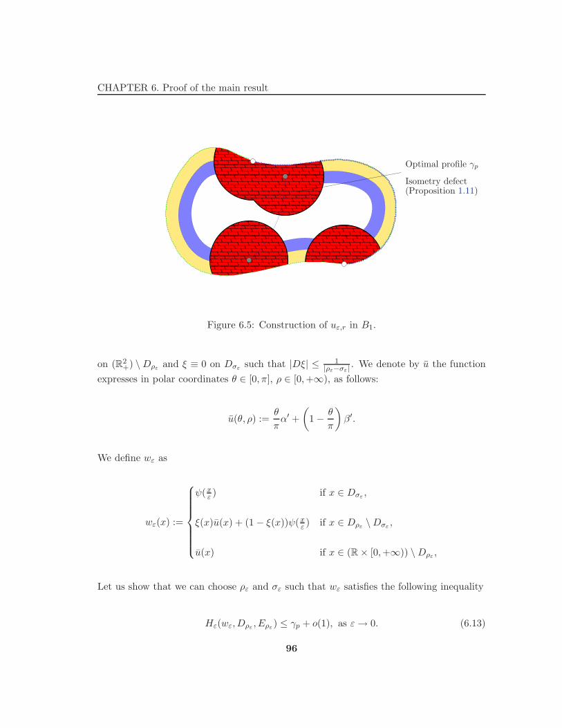
CHAPTER 6. Proof of the main result
Optimal profile γp
Isometry defect(Proposition 1.11)
Figure 6.5: Construction of uε,r in B1.
on (R2+) \Dρε and ξ ≡ 0 on Dσε such that |Dξ| ≤ 1
|ρε−σε|. We denote by u the function
expresses in polar coordinates θ ∈ [0, π], ρ ∈ [0,+∞), as follows:
u(θ, ρ) :=θ
πα′ +
(
1 − θ
π
)
β′.
We define wε as
wε(x) :=
ψ(xε ) if x ∈ Dσε ,
ξ(x)u(x) + (1 − ξ(x))ψ(xε ) if x ∈ Dρε \Dσε ,
u(x) if x ∈ (R × [0,+∞)) \Dρε ,
Let us show that we can choose ρε and σε such that wε satisfies the following inequality
Hε(wε,Dρε , Eρε) ≤ γp + o(1), as ε→ 0. (6.13)
96
CHAPTER 6. Proof of the main result
We have
Hε(wε,Dρε , Eρε) = Hε(ψ(ε),Dσε , Eσε) + εp−2
∫
Dρε\Dσε
|Dwε|pdx
+1
ε
∫
Eρε\Eσε
V (Twε)dH1
(6.14)
=: Hε(ψ(ε),Dσε , Eσε) + I1 + I2,
where ψ(ε)(x) := ψ(xε ) (see Section 5.3, p. 72).
The first integral in the right hand side of (6.14) can be easily estimated as follows
I1 ≤ 3p−1εp−2
∫
Dρε\Dσε
|Dψ(x
ε)|pdx+ 3p−1εp−2
∫
Dρε\Dσε
|Dξ|p|ψ(x
ε) − u(x)|pdx
+3p−1εp−2
∫
Dρε\Dσε
|Du|pdx
(6.15)
≤ 3p−1
∫
Dρε/ε\Dσε/ε
|Dψ|pdx+ 3p−1Cpεp−2(ρ2
ε − σ2ε)
(ρε − σε)p+
3p−1|β′ − α′|p(p − 2)πp−1
(
ε
σε
)p−2
.
While using the convexity of V near its wells and the asymptotic behavior of Tψ(xε ), for
ε small, we have
I2 ≤ 1
ε
∫
Dρε\Dσε
V (Tψ(x
ε))dH1. (6.16)
Thus, by (6.14), (6.15), (6.16) and suitably choosing of ρε and σε1, we get
Hε(wε,Dρε , Eρε) ≤ Hε(ψ(ε),Dρε , Eρε) + 3p−1
∫
Dρε/ε\Dσε/ε
|Dψ|pdx+ 3p−1Cpεp−2(ρ2
ε − σ2ε)
(ρε − σε)p
+3p−1|β′ − α′|p(p− 2)πp−1
(
ε
ρε
)p−2
(6.17)
≤ γp + o(1) as ε→ 0.
We now define a function wε on Sv × R2+, by
wε(x, y) := wε(x), for every x ∈ Sv and every y ∈ R2+. (6.18)
1For instance, we can choose ρε = ε1/3 + ε1/2 and σε = ε1/2.
97

CHAPTER 6. Proof of the main result
Using (6.17) and Fubini’s Theorem, we obtain2
Fε(wε, Sv×Dρε , Sv×Eρε) = H1(Sv)
(
Hε(wε,Dρε , Eρε) +1
ε(p−2)/(p−1)
∫
Dρε
W (wε)dx
)
≤ H1(Sv)(
γp + o(1))
as ε→ 0. (6.19)
Since Sv is a boundary in ∂Ω, we can construct a diffeomorfism between the intersection
of a tubular neighborhood of Sv and Ω and the product of Sv with an half-disk.
For every x in Ω, let us define the oriented distance from Sv as
d′(x) :=
dist(x, Sv) if x ∈ v = β′,
−dist(x, Sv) if x ∈ v = α′.
For every r > 0, we set
Sr := x ∈ Ω : 0 < dist(x, Sv) < r . (6.20)
For every x ∈ Ω, we define
Ψ(x) := (x′′, d′(x′),dist(x, ∂Ω)), (6.21)
where x′ is a projection of x on ∂Ω and x′′ is a projection of x′ on Sv. The function Ψ is
well-defined and is a diffeomorfism of class C2 on Ω ∩U for some neighborhood U of Sv;
and satisfies the following properties: Ψ(Ω ∩ U) = Sv × R2+; Ψ(∂Ω ∩ U) = Sv × R × 0;
Ψ(x) = x, for every x ∈ ∂Ω; DΨ(x) is an isometry.
We have that
limr→0
δr = 0,
where δr is the isometry defect of the restriction of Ψ to Sr (see Section 1.3.2).
We construct uε,r on Sρε/2 as
uε,r := wε Ψ,
where wε, Sr and Ψ are defined by (6.18), (6.20) and (6.21) respectively. For ε small,
the function Ψ maps Sρε/2 into Sv ×Dρε and ∂Sρε/2 ∩ ∂Ω into Sv × Eρε , so we can use
2Note that we can define the functional Fε by (6.1) also on functions u ∈ W 1,p(A), where A ⊂ RN ,
with N ≥ 3.
98
CHAPTER 6. Proof of the main result
Proposition 1.11 and, by (6.19), we obtain
Fε(uε,r,Sρε/2, ∂Sρε/2 ∩ ∂Ω) ≤ (1 − δε)−(p+3)Fε(wε, Sv ×Dρε , Sv × Eρε)
(6.22)
≤ H1(Sv)(
γp + o(1))
as ε→ 0,
where we also used that δε := δ(Ψ⌊Sρε) tends to 0 as ε→ 0.
Notice that for ε small enough, Ψ is 2-Lipschitz continuous. Using again Lemma 6.2,
we can extend uε,r by setting uε,r := v on the remaining part of ∂B1 ∩ ∂Ω; we have that
uε,r is equal to v on ∂Ω \ ∂Sρε/2. Thus, we can extend uε,r on the whole B1 \ Sρε/2 to a2C + 1
ε(p−2)/(p−1)-Lipschitz continuous function, which satisfies
Fε(uε,r, B1\Sρε/2, ∂(B1\Sρε/2) ∩ ∂Ω) = Gε(uε,r, B1 \ Sρε/2)
(6.23)
≤(
(2C + 2)p+ Cm)(
H2(∂B1) + o(1))
2m as ε→ 0,
where we used ‖uε,r − α‖∞ ∧ ‖uε,r − β‖∞ ≤ 2m.
Step 6: Upper bound inequality. We recall that for every r > 0 and every ε < rp−2p−1 we
have constructed a function uε,r defined on the whole Ω such that
lim supε→0
‖uε,r − u‖L1(Ω) ≤ 2m(|B1| + |B2|) and lim supε→0
‖Tuε,r − v‖L1(∂Ω) = 0.
Since |B1| and |B2| have order r2 and r respectively, we get that uε,r → u in L1(Ω), first
taking ε→ 0 and then r → 0.
Combining (6.10), (6.11), (6.12), (6.22) and (6.23), we obtain
lim supε→0
Fε(uε,r) ≤ σpH2(Su) + cp
∫
∂Ω|W(Tu(x)) −W(v(x))|dH2 + γpH1(Sv)
(6.24)
−σpH2(Su \A2) +(
(2C + 2)p+ Cm)(
H2(∂B1) + o(1))
2m.
Since H2(∂B1) has order r, taking r to 0 in (6.24), we deduce the upper bound
inequality (iii). Finally, applying a suitable diagonalization argument3 to the sequence
uε,r, we obtain the desired recovery sequence uε. This concludes the proof. 2
3See for instance Attouch [12], Corollary 1.18, p. 37.
99

List of Symbols
Sets, numbers, measures
a ∨ b (a ∧ b) the maximum (minimum) between a and b
Br(x) the open ball of centre x and radius r
C (if not otherwise stated) a strictly positive constant independent from the parameters
|E| the Lebesgue measure of the set E
Hk the k-dimensional Hausdorff measure
µ E the restriction of the measure µ to E
[t] the integer part of t ∈ R
Function spaces
O(3) the set of linear isometries on R3
Ck(Ω) the space of k-times differentiable real valued functions on Ω
C0(R) the closure of continuous functions on R with compact support
M(R) (M+(R)) the space of signed (positive) Radon measure with finite mass
P(R) the set of probability measures on R.
Y(A) the family of all weakly-∗ measurable maps ν : A→ P(R)
Lp(Ω) the space of real valued p-summable functions on Ω
W 1,p(Ω) the space of Sobolev functions with p-summable derivatives on Ω
‖u‖Lp(Ω) or simply ‖u‖p the Lp norm of u
‖u‖W 1,p(Ω) the W 1,p norm of u
W k,p(ω) the fractional space of order k, s of functions on ω
‖v‖W k,p(ω) or simply ‖v‖k,p the W k,p norm of v
Xloc(Ω) u : Ω → R : u ∈ X(A) for all open A ⊂⊂ Ω, where X is a generic notation for
a function space
100
LIST OF SYMBOLS
Functions
χE the characteristic function of the set E(
χE(x) = 1 if x ∈ E, χE(x) = 0 if x /∈ E)
Su the set of essential discontinuity points of u (jump set)
νu(x) the normal to Su at x
un → u un converges strongly to u
un u un converges weakly to u
un∗ u un converges weakly-∗ to u
101
List of Figures
0.1 A two-phase system. . . . . . . . . . . . . . . . . . . . . . . . . . . . . . . 6
0.2 A double-well type potential W . . . . . . . . . . . . . . . . . . . . . . . . 7
0.3 The line tension effect. . . . . . . . . . . . . . . . . . . . . . . . . . . . . . 9
0.4 An arbitrary configuration (A,A′). . . . . . . . . . . . . . . . . . . . . . . 10
1.1 A section of the domain A. . . . . . . . . . . . . . . . . . . . . . . . . . . 25
1.2 Construction of Ψ := Ψ−11 Ψ2 Ψ1 ([9], Fig. 5, p. 26). . . . . . . . . . . 29
2.1 The classical model for phase transitions. . . . . . . . . . . . . . . . . . . 33
2.2 A double-well type potential W . . . . . . . . . . . . . . . . . . . . . . . . 34
2.3 The line tension effect. . . . . . . . . . . . . . . . . . . . . . . . . . . . . . 38
2.4 An arbitrary configuration (A,A′). . . . . . . . . . . . . . . . . . . . . . . 40
3.1 The competitor ϕ. . . . . . . . . . . . . . . . . . . . . . . . . . . . . . . . 48
3.2 Construction of vε, with I = (a, b) and H0(Sv) = 3. . . . . . . . . . . . . . 59
4.1 The bulk. . . . . . . . . . . . . . . . . . . . . . . . . . . . . . . . . . . . . 63
4.2 The wall. . . . . . . . . . . . . . . . . . . . . . . . . . . . . . . . . . . . . 63
4.3 The boundary. . . . . . . . . . . . . . . . . . . . . . . . . . . . . . . . . . 69
5.1 The competitor wε. . . . . . . . . . . . . . . . . . . . . . . . . . . . . . . . 75
5.2 The sets D,E,Ee, Ey and Dy. . . . . . . . . . . . . . . . . . . . . . . . . . 79
5.3 The competitor u. . . . . . . . . . . . . . . . . . . . . . . . . . . . . . . . 83
6.1 Upper bound inequality - partition of Ω. . . . . . . . . . . . . . . . . . . . 92
6.2 Construction of uε,r in A2. . . . . . . . . . . . . . . . . . . . . . . . . . . . 93
6.3 Construction of uε,r in A1. . . . . . . . . . . . . . . . . . . . . . . . . . . . 94
6.4 Construction of uε,r in B2. . . . . . . . . . . . . . . . . . . . . . . . . . . . 95
6.5 Construction of uε,r in B1. . . . . . . . . . . . . . . . . . . . . . . . . . . . 96
102

Bibliography
[1] R. Adams and J. J. F. Fournier, Sobolev Spaces (second edition). Academic
Press, Oxford, 2003.
[2] G. Alberti, Variational models for phase transitions, an approach via Gamma-
convergence, in L. Ambrosio and N. Dancers, Calculus of variations and partial
differential equations, G. Buttazzo et al., Eds., Springer-Verlag, Berlin, 2000, pp.
95-114.
[3] G. Alberti, Some remarks about a notion of rearrangement, Ann. Scuola Norm.
Sup. Pisa Cl. Sci., 4 (2000), pp. 457-472.
[4] G. Alberti, S. Baldo and G. Orlandi, Variational convergence for functionals
of Ginzburg-Landau type, Indiana Univ. Math. J., 5 (2003), pp. 275-311.
[5] G. Alberti and G. Bellettini, A nonlocal anisotropic model for phase transitions
I: the optimal profile problem, Math. Ann., 310 (1998), pp. 527-560.
[6] G. Alberti and G. Bellettini, A nonlocal anisotropic model for phase transi-
tions: asymptotic behavior of rescaled energies, European Journal of Applied Math-
ematics, 9 (1998), pp. 261-284.
[7] G. Alberti, G. Bouchitte and P. Seppecher, Boundary effects in phase tran-
sitions, in Curvature Flows and Related Topics, A. Visintin, Ed., Gakkatosho, Tokio,
1995, pp. 1-11.
[8] G. Alberti, G. Bouchitte and P. Seppecher, Un resultat de perturbations
singulieres avec la norme H1/2, C. R. Acad. Sci. Paris, Serie I, 319 (1994), pp.
333-338.
[9] G. Alberti, G. Bouchitte and P. Seppecher, Phase Transition with Line-
Tension Effect, Arch. Rational Mech. Anal., 144 (1998), pp. 1-46.
103

BIBLIOGRAPHY
[10] L. Ambrosio, N. Fusco and D. Pallara, Functions of bounded variation and
free discontinuity problems, Oxford Mathematical monographs, Oxford, 2000.
[11] G. Anzellotti and M. Giaquinta, Funzioni BV e tracce, Rend. Sem. Mat. Univ.
Padova, 60 (1978), pp. 1-21.
[12] H. Attouch, Variational Convergence for Functions and Operators, Pitman,
Boston, 1984.
[13] J. M. Ball, A version of the fundamental theorem for Young measures, in PDEs
and continuum models of phase transitions (Nice, 1988), M. Rascle, D. Serre and
M. Slemrod, Eds., Lecture Notes in Phys., 344, Springer-Verlag, Berlin, 1989, pp.
207-215.
[14] C. Bandle, Isoperimetric inequalities and applications, Pitman, Boston, 1980.
[15] A. Baernstein II, A unified approach to symmetrization, in Partial Differential
Equations of Elliptic type (Cortona, 1992), Sympos. Math., XXXV, Cambridge Uni-
versity Press, Cambridge, 1994, pp. 47-91.
[16] A. C. Barroso and I. Fonseca, Anisotropic singular perturbations: the vectorial
case, Proc. Roy. Soc. Edinburgh Sect. A, 124 (1994), no. 3, pp. 527-571.
[17] H. Berestycki and T. Lachand-Robert, Some properties of monotone rear-
rangement with applications to elliptic equations in cylinders, Math. Nachr., 266
(2004), pp. 3-19.
[18] F. Bethuel, H. Brezis and F. Helein, Ginzburg-Landau vortices. Progress
in NonLinear Differential Equations and Their Applications, Vol. 13, Birkhauser,
Boston, 1994.
[19] G. Bouchitte, Singular perturbations of variational problems arising from a two-
phase transition model, Appl. Math. Opt., 21 (1990), pp. 289-315.
[20] A. Braides, A handbook of Γ-convergence, in Handbook of Differential Equations,
Vol. 3, M. Chipot and P. Quittner, Eds., Elsevier, Amsterdam, 2006.
[21] A. Braides, A short introduction to Young Measures, Lecture Notes, SISSA, Trieste,
2000.
[22] A. Braides, Approximation of Free-Discontinuity Problems, Lecture Notes in Math-
ematics No. 1694, Springer Verlag, Berlin, 1998.
104
BIBLIOGRAPHY
[23] A. Braides, Γ-convergence for beginners, Oxford University Press, Oxford, 2002.
[24] J. W. Cahn, Critical point wetting, J. Chem. Phys., Vol. 66, 8 (1977), pp. 3667-3672.
[25] J. W. Cahn and J. E. Hilliard, Free energy of a nonuniform system. I. Interfacial
free energy, J. Chem. Phys., Vol. 28, 2 (1958), p. 258-267.
[26] J. W. Cahn and R. B. Heady, Experimental test of classical nucleation theory in
a liquid-liquid miscibility gap system, J. Chem. Phys., Vol. 58, 2 (1973), p. 896-910.
[27] G. Dal Maso, An introduction to Γ-convergence, Progress in Nonlinear Differential
Equations and their Application, 8, Birkhauser, Boston, 1993.
[28] E. De Giorgi and T. Franzoni, Su un tipo di convergenza variazionale, Atti
Accad. Naz. Lincei Rend. Cl. Sci. Fis. Mat. Natur., Vol. VIII, 58 (1975), pp. 842-
850.
[29] N. Desenzani and I. Fragala, Concentration of Ginzburg-Landau energies with
“supercritical” growth, SIAM J. Math. Anal., 38 (2006), pp. 385-416.
[30] N. Desenzani and I. Fragala, Asymptotics of boundary value problems for super-
critical Ginzburg-Landau energies, in Variational problems in materials science, G.
Dal Maso, A. De Simone and F. Tomarelli, Eds., Progress in NonLinear Differential
Equations and Their Applications, Vol. 68, Birkhauser, Basel, 2006, pp. 75-84.
[31] L. C. Evans., Weak convergence methods for nonlinear partial differential equations,
CBMS Regional Conference Series in Mathematics, 74, Conference Board of the
Mathematical Sciences, Washington, 1990.
[32] L. C. Evans and R. F. Gariepy, Measure Theory and Fine Properties of Func-
tions, CRC Press, Boca Raton, 1992.
[33] R. Finn, Equilibrium Capillary Surfaces, Springer, New York 1986.
[34] I. Fonseca, Remarks on phase transitions, in Recent advances in nonlinear elliptic
and parabolic problems (Nancy, 1988), 208, Pitman Res. Notes Math. Ser., Longman
Sci. Tech., Harlow, 1989, pp. 274-282.
[35] I. Fonseca and C. Mantegazza, Second order singular perturbation models for
phase transitions, SIAM J. Math. Anal., 31(5) (2000), p. 1121-1143.
[36] I. Fonseca and S. Muller, Quasiconvex integrands and lower semicontinuity in
L1, SIAM J. Math. Anal., 23(5) (1992), pp. 1081-1098.
105

BIBLIOGRAPHY
[37] I. Fonseca and L. Tartar, The gradient theory of phase transitions for systems
with two potential wells, Proc. Roy. Soc. Edinburgh Sect. A, 111 (1989), pp. 89-102.
[38] A. M. Garsia and E. Rodemich, Monotonicity of certain functionals under rear-
rangement, Ann. Inst. Fourier, 24 (1974), pp. 67-116.
[39] A. Garroni and S. Muller, A variational model for dislocations in the line tension
limit, Arch. Rational Mech. Anal., 181 (2006), pp. 535-578.
[40] A. Garroni and G. Palatucci, A singular perturbation result with a fractional
norm, in Variational problems in material science, G. Dal Maso, A. De Simone and
F. Tomarelli, Eds., Progress in NonLinear Differential Equations and Their Applica-
tions, Vol. 68, Birkhauser, Basel, 2006, pp. 111-126.
[41] J. W. Gibbs, The collected papers of J. Willard Gibbs, Yale University Press, Lon-
don, 1957.
[42] E. Giusti, Minimal surfaces and functions of bounded variation, Birkhauser, Basel,
1984.
[43] M. E. Gurtin, On a theory of phase transitions and the minimal interface criterion.
Arch. Rational Mech. Anal., 87 (1984), pp. 187-212.
[44] G. H. Hardy, J. E. Littlewood and G. Polya, Inequalities, Cambridge Univ.
Press, Cambridge, 1958.
[45] B. Kawohl, Rearrangements and convexity of level sets in PDE, Springer-Verlag,
Berlin, 1985.
[46] M. Kurzke, A nonlocal singular perturbation problem with periodic well potential,
ESAIM: COCV, 12 (2006), pp. 52-63.
[47] M. Kurzke, Boundary vortices in thin magnetic films, Calc. Var., 26 (2006), pp.
1-28.
[48] L. Modica, Gradient theory of phase transitions and minimal interface criterion,
Arch. Rational Mech. Anal., 98 (1987), pp. 123-142.
[49] L. Modica, Gradient theory of phase transitions with boundary contact energy,
Ann. Inst. H. Poincare Anal. Non Lineaire, 5 (1987), pp. 453-486.
[50] L. Modica and S. Mortola, Un esempio di Γ−-convergenza, Boll. Un. Mat. Ital.
B(5), 14 (1977), pp. 285-299.
106
BIBLIOGRAPHY
[51] U. Mosco, Convergence of convex sets and of solutions of variational inequalities,
Adv. Math., 3 (1969), pp. 510-585.
[52] S. Muller, Microstructures, phase transitions and geometry, in European Congress
of Mathematics (Budapest, 1996), A. Balog et al., Eds, Progress in Mathematics,
Vol. 169, Birkhauser, Basel, 1998, pp. 92-115.
[53] S. Muller, Variational models for microstructure and phase transitions, in Calculus
of variations and geometric evolution problems (Proc. C.I.M.E., Cetraro, 1996), F.
Bethuel et al., Eds., Lecture Notes in Math. 1713, Springer-Verlag, Berlin, 1999, pp.
85-210.
[54] N. Owen and P. Sternberg, Nonconvex variational problems with anisotropic
perturbations, Nonlinear Anal. T.M.A., 16 (1991), pp. 705-719.
[55] B. Sousa, PhD Thesis, in preparation.
[56] M. Valadier, Young Measures in Methods of Nonconvex Analysis, Lecture Notes
in Math., Springer-Verlag, 1446 (1990), pp. 152-188.
[57] M. Valadier, A course on Young measures, Rend. Isti. Mat. Univ. Trieste, 26
(1994) suppl., pp. 349-394.
[58] L. C. Young, Generalized curves and the existence of an attained absolute minimum
in the calculus of variations, C.R. Soc. Sci. Lettres de Varsovie, Cl. III , 30 (1937)
pp. 212-234.
107

Giampiero PalatucciDipartimento di Matematica,Universita degli Studi “Roma Tre”,L.go S. Leonardo Murialdo, 1,00146, Roma, Italiae-mail: [email protected]