A CLASS OF MEASURABLE DYNAMICALSYSTEMS FOR CHAOTIC CRYPTOGRAPHY

AFSHIN AKHSHANI

UNIVERSITI SAINS MALAYSIA2008

A CLASS OF MEASURABLE DYNAMICALSYSTEMS FOR CHAOTIC CRYPTOGRAPHY

by

AFSHIN AKHSHANI

Thesis submitted in fulfilment of the requirementsfor the degree of

Master of Science

April 2008

ACKNOWLEDGEMENTS

First and foremost, I have to thank God for somehow turning an innumerable amount of

seemingly hard into an easy and golden decisions. I would like to take this opportunity to

express my deepest gratitude to my dear supervisors, Dr. Zainuriah Hassan and Dr. Haslan Abu

Hassan for the support they have given to me from the beginning of my research in the School

of Physics. A special thanks to Dr. Sohrab Behnia for providing me with valuable insight and

comments towards the end of my work. I would like to thank Professor Mohammad Ali Ja-

farizadeh for his enormously creative directions which inspired me along my research. Finally,

I would like to extend a heartfelt thanks to my supportive parents, brother and sister. But most

importantly, my deepest love. Without their constant and unconditional support and love, none

of my accomplishments would be possible. To them, I dedicate this thesis.

ii

TABLE OF CONTENTS

Acknowledgements . . . . . . . . . . . . . . . . . . . . . . . . . . . . . . . . . . . . . . . . . . . . . . . . . . . . . . . . . . . . . . . . . . . . . . . . . . . ii

Table of Contents . . . . . . . . . . . . . . . . . . . . . . . . . . . . . . . . . . . . . . . . . . . . . . . . . . . . . . . . . . . . . . . . . . . . . . . . . . . . . iii

List of Tables . . . . . . . . . . . . . . . . . . . . . . . . . . . . . . . . . . . . . . . . . . . . . . . . . . . . . . . . . . . . . . . . . . . . . . . . . . . . . . . . . . vii

List of Figures . . . . . . . . . . . . . . . . . . . . . . . . . . . . . . . . . . . . . . . . . . . . . . . . . . . . . . . . . . . . . . . . . . . . . . . . . . . . . . . . viii

List of Abbreviations . . . . . . . . . . . . . . . . . . . . . . . . . . . . . . . . . . . . . . . . . . . . . . . . . . . . . . . . . . . . . . . . . . . . . . . . . x

List of Symbols . . . . . . . . . . . . . . . . . . . . . . . . . . . . . . . . . . . . . . . . . . . . . . . . . . . . . . . . . . . . . . . . . . . . . . . . . . . . . . . xi

Abstrak . . . . . . . . . . . . . . . . . . . . . . . . . . . . . . . . . . . . . . . . . . . . . . . . . . . . . . . . . . . . . . . . . . . . . . . . . . . . . . . . . . . . . . . . xiii

Abstract . . . . . . . . . . . . . . . . . . . . . . . . . . . . . . . . . . . . . . . . . . . . . . . . . . . . . . . . . . . . . . . . . . . . . . . . . . . . . . . . . . . . . . . xv

CHAPTER 1 – INTRODUCTION

1.1 Research Background. . . . . . . . . . . . . . . . . . . . . . . . . . . . . . . . . . . . . . . . . . . . . . . . . . . . . . . . . . . . . . . . . . 1

1.2 Research Objectives . . . . . . . . . . . . . . . . . . . . . . . . . . . . . . . . . . . . . . . . . . . . . . . . . . . . . . . . . . . . . . . . . . . 2

1.3 Organization of Thesis. . . . . . . . . . . . . . . . . . . . . . . . . . . . . . . . . . . . . . . . . . . . . . . . . . . . . . . . . . . . . . . . . 3

CHAPTER 2 – LITERATURE REVIEW

2.1 Dynamical Systems . . . . . . . . . . . . . . . . . . . . . . . . . . . . . . . . . . . . . . . . . . . . . . . . . . . . . . . . . . . . . . . . . . . . 4

2.1.1 Nonlinear dynamics . . . . . . . . . . . . . . . . . . . . . . . . . . . . . . . . . . . . . . . . . . . . . . . . . . . . . . . . . . 4

2.1.2 Linear system . . . . . . . . . . . . . . . . . . . . . . . . . . . . . . . . . . . . . . . . . . . . . . . . . . . . . . . . . . . . . . . . . 4

2.1.3 Nonlinear system . . . . . . . . . . . . . . . . . . . . . . . . . . . . . . . . . . . . . . . . . . . . . . . . . . . . . . . . . . . . . 5

2.2 Chaos . . . . . . . . . . . . . . . . . . . . . . . . . . . . . . . . . . . . . . . . . . . . . . . . . . . . . . . . . . . . . . . . . . . . . . . . . . . . . . . . . . . 6

2.3 Invariant Measure . . . . . . . . . . . . . . . . . . . . . . . . . . . . . . . . . . . . . . . . . . . . . . . . . . . . . . . . . . . . . . . . . . . . . . 7

2.4 Frobenius-Perron Operator . . . . . . . . . . . . . . . . . . . . . . . . . . . . . . . . . . . . . . . . . . . . . . . . . . . . . . . . . . . . 10

2.5 Ergodic Theory. . . . . . . . . . . . . . . . . . . . . . . . . . . . . . . . . . . . . . . . . . . . . . . . . . . . . . . . . . . . . . . . . . . . . . . . . 11

2.6 Lyapunov Exponent. . . . . . . . . . . . . . . . . . . . . . . . . . . . . . . . . . . . . . . . . . . . . . . . . . . . . . . . . . . . . . . . . . . . 12

2.7 Kolmogorov-Sinai Entropy . . . . . . . . . . . . . . . . . . . . . . . . . . . . . . . . . . . . . . . . . . . . . . . . . . . . . . . . . . . . 14

2.8 Fractal Dimension . . . . . . . . . . . . . . . . . . . . . . . . . . . . . . . . . . . . . . . . . . . . . . . . . . . . . . . . . . . . . . . . . . . . . 15

iii

2.9 Bifurcation . . . . . . . . . . . . . . . . . . . . . . . . . . . . . . . . . . . . . . . . . . . . . . . . . . . . . . . . . . . . . . . . . . . . . . . . . . . . . 15

2.10 Attractors . . . . . . . . . . . . . . . . . . . . . . . . . . . . . . . . . . . . . . . . . . . . . . . . . . . . . . . . . . . . . . . . . . . . . . . . . . . . . . . 15

2.11 Fixed Point . . . . . . . . . . . . . . . . . . . . . . . . . . . . . . . . . . . . . . . . . . . . . . . . . . . . . . . . . . . . . . . . . . . . . . . . . . . . . 17

2.12 Chaotic Maps . . . . . . . . . . . . . . . . . . . . . . . . . . . . . . . . . . . . . . . . . . . . . . . . . . . . . . . . . . . . . . . . . . . . . . . . . . 18

CHAPTER 3 – ONE-PARAMETER FAMILIES OF CHAOTIC MAPS

3.1 One-parameter families of chaotic maps . . . . . . . . . . . . . . . . . . . . . . . . . . . . . . . . . . . . . . . . . . . . . 19

3.2 Numerical Simulations . . . . . . . . . . . . . . . . . . . . . . . . . . . . . . . . . . . . . . . . . . . . . . . . . . . . . . . . . . . . . . . . 20

CHAPTER 4 – HIERARCHY OF 2D PIECEWISE NONLINEAR CHAOTICMAPS

4.1 Two Dimensional Piecewise Nonlinear Chaotic Maps. . . . . . . . . . . . . . . . . . . . . . . . . . . . . . . 24

4.1.1 Invariant measure for 2D piecewise nonlinear chaotic maps . . . . . . . . . . . . . . . 25

4.1.2 K-S entropy for 2D piecewise nonlinear chaotic maps . . . . . . . . . . . . . . . . . . . . . 29

4.1.3 Numerical simulations. . . . . . . . . . . . . . . . . . . . . . . . . . . . . . . . . . . . . . . . . . . . . . . . . . . . . . . . 30

CHAPTER 5 – INTRODUCTION TO CHAOTIC CRYPTOGRAPHY

5.1 Cryptographic Techniques . . . . . . . . . . . . . . . . . . . . . . . . . . . . . . . . . . . . . . . . . . . . . . . . . . . . . . . . . . . . . 33

5.2 Ciphers . . . . . . . . . . . . . . . . . . . . . . . . . . . . . . . . . . . . . . . . . . . . . . . . . . . . . . . . . . . . . . . . . . . . . . . . . . . . . . . . . 33

5.3 Encryption. . . . . . . . . . . . . . . . . . . . . . . . . . . . . . . . . . . . . . . . . . . . . . . . . . . . . . . . . . . . . . . . . . . . . . . . . . . . . . 34

5.4 Symmetric and Asymmetric-key Algorithms. . . . . . . . . . . . . . . . . . . . . . . . . . . . . . . . . . . . . . . . . 34

5.4.1 Block ciphers and stream ciphers . . . . . . . . . . . . . . . . . . . . . . . . . . . . . . . . . . . . . . . . . . . . 35

5.4.2 Pseudo-random number generators . . . . . . . . . . . . . . . . . . . . . . . . . . . . . . . . . . . . . . . . . . 36

5.4.3 Hash functions . . . . . . . . . . . . . . . . . . . . . . . . . . . . . . . . . . . . . . . . . . . . . . . . . . . . . . . . . . . . . . . . 37

5.5 Connection Between Chaos and Cryptography Properties . . . . . . . . . . . . . . . . . . . . . . . . . . 38

5.6 Cryptanalysis . . . . . . . . . . . . . . . . . . . . . . . . . . . . . . . . . . . . . . . . . . . . . . . . . . . . . . . . . . . . . . . . . . . . . . . . . . . 38

CHAPTER 6 – HASH FUNCTION BASED ON 2D PIECEWISE NONLINEARCHAOTIC MAPS

6.1 Proposed Algorithm . . . . . . . . . . . . . . . . . . . . . . . . . . . . . . . . . . . . . . . . . . . . . . . . . . . . . . . . . . . . . . . . . . . 41

iv

6.2 Performance Analysis . . . . . . . . . . . . . . . . . . . . . . . . . . . . . . . . . . . . . . . . . . . . . . . . . . . . . . . . . . . . . . . . . 42

6.2.1 Hash results of messages . . . . . . . . . . . . . . . . . . . . . . . . . . . . . . . . . . . . . . . . . . . . . . . . . . . . . 42

6.2.2 Statistical analysis of diffusion and confusion . . . . . . . . . . . . . . . . . . . . . . . . . . . . . . 44

6.2.3 Analysis of collision resistance and birthday attacks resistance. . . . . . . . . . . . 45

6.2.4 Meet-in-the-middle attack . . . . . . . . . . . . . . . . . . . . . . . . . . . . . . . . . . . . . . . . . . . . . . . . . . . . 49

6.2.5 Flexibility . . . . . . . . . . . . . . . . . . . . . . . . . . . . . . . . . . . . . . . . . . . . . . . . . . . . . . . . . . . . . . . . . . . . . 49

6.2.6 Security of key . . . . . . . . . . . . . . . . . . . . . . . . . . . . . . . . . . . . . . . . . . . . . . . . . . . . . . . . . . . . . . . . 49

6.2.7 Analysis of speed . . . . . . . . . . . . . . . . . . . . . . . . . . . . . . . . . . . . . . . . . . . . . . . . . . . . . . . . . . . . . 50

6.2.8 Uniform distribution on hash space . . . . . . . . . . . . . . . . . . . . . . . . . . . . . . . . . . . . . . . . . . 50

6.3 Performance Comparison. . . . . . . . . . . . . . . . . . . . . . . . . . . . . . . . . . . . . . . . . . . . . . . . . . . . . . . . . . . . . . 52

6.3.1 Statistical analysis . . . . . . . . . . . . . . . . . . . . . . . . . . . . . . . . . . . . . . . . . . . . . . . . . . . . . . . . . . . . 52

6.3.2 Collision resistance . . . . . . . . . . . . . . . . . . . . . . . . . . . . . . . . . . . . . . . . . . . . . . . . . . . . . . . . . . . 52

6.3.3 Speed analysis . . . . . . . . . . . . . . . . . . . . . . . . . . . . . . . . . . . . . . . . . . . . . . . . . . . . . . . . . . . . . . . . 53

6.3.4 Further discussion . . . . . . . . . . . . . . . . . . . . . . . . . . . . . . . . . . . . . . . . . . . . . . . . . . . . . . . . . . . . 53

6.4 Summary . . . . . . . . . . . . . . . . . . . . . . . . . . . . . . . . . . . . . . . . . . . . . . . . . . . . . . . . . . . . . . . . . . . . . . . . . . . . . . . 54

CHAPTER 7 – A NOVEL SCHEME FOR IMAGE ENCRYPTION BASED ON 2DPIECEWISE NONLINEAR CHAOTIC MAPS

7.1 Proposed Algorithm . . . . . . . . . . . . . . . . . . . . . . . . . . . . . . . . . . . . . . . . . . . . . . . . . . . . . . . . . . . . . . . . . . . 58

7.2 Experimental Results . . . . . . . . . . . . . . . . . . . . . . . . . . . . . . . . . . . . . . . . . . . . . . . . . . . . . . . . . . . . . . . . . . 59

7.3 Security Analysis . . . . . . . . . . . . . . . . . . . . . . . . . . . . . . . . . . . . . . . . . . . . . . . . . . . . . . . . . . . . . . . . . . . . . . 60

7.3.1 Key space analysis . . . . . . . . . . . . . . . . . . . . . . . . . . . . . . . . . . . . . . . . . . . . . . . . . . . . . . . . . . . . 62

7.3.2 Key sensitivity . . . . . . . . . . . . . . . . . . . . . . . . . . . . . . . . . . . . . . . . . . . . . . . . . . . . . . . . . . . . . . . . 62

7.3.3 Sensitivity to the plain image . . . . . . . . . . . . . . . . . . . . . . . . . . . . . . . . . . . . . . . . . . . . . . . . 63

7.3.4 Statistical analysis . . . . . . . . . . . . . . . . . . . . . . . . . . . . . . . . . . . . . . . . . . . . . . . . . . . . . . . . . . . . 63

7.3.5 Information entropy . . . . . . . . . . . . . . . . . . . . . . . . . . . . . . . . . . . . . . . . . . . . . . . . . . . . . . . . . . 70

7.3.6 Differential attack. . . . . . . . . . . . . . . . . . . . . . . . . . . . . . . . . . . . . . . . . . . . . . . . . . . . . . . . . . . . . 72

7.3.7 Analysis of speed . . . . . . . . . . . . . . . . . . . . . . . . . . . . . . . . . . . . . . . . . . . . . . . . . . . . . . . . . . . . . 73

v

7.4 Summary . . . . . . . . . . . . . . . . . . . . . . . . . . . . . . . . . . . . . . . . . . . . . . . . . . . . . . . . . . . . . . . . . . . . . . . . . . . . . . . 74

CHAPTER 8 – CONCLUSION AND FUTURE WORK

References . . . . . . . . . . . . . . . . . . . . . . . . . . . . . . . . . . . . . . . . . . . . . . . . . . . . . . . . . . . . . . . . . . . . . . . . . . . . . . . . . . . . . 77

APPENDICES . . . . . . . . . . . . . . . . . . . . . . . . . . . . . . . . . . . . . . . . . . . . . . . . . . . . . . . . . . . . . . . . . . . . . . . . . . . . . . . . . 82

APPENDIX A – INVARIANT MEASURE FOR ONE-PARAMETER FAMILIESOF CHAOTIC MAPS . . . . . . . . . . . . . . . . . . . . . . . . . . . . . . . . . . . . . . . . . . . . . . . . . . . . 83

vi

LIST OF TABLES

Page

Table 2.1 Lyapunov exponents of chaotic maps 13

Table 5.1 Connections between chaos and cryptography 38

Table 6.1 Static number of changed bit Bi 45

Table 6.2 Maximum, minimum and mean values of the absolute difference (d)of two hash values, 128-bits 47

Table 6.3 Maximum, minimum and mean values of the absolute difference (d)of two hash values, 160-bits 47

Table 6.4 A comparison of maximum, minimum and mean values of theabsolute difference (d) of two hash values 53

Table 6.5 Required multiplicative operation for each byte of message 54

Table 7.1 Correlation coefficient of two adjacent pixels in two images 70

vii

LIST OF FIGURES

Page

Figure 2.1 Logistic map transformation. 10

Figure 2.2 Lyapunov exponent of Logistic map 13

Figure 2.3 Bifurcation diagram of Logistic map 16

Figure 2.4 Attractor 17

Figure 3.1 Bifurcation diagram of Φ(1)4 (x,α) 20

Figure 3.2 Bifurcation diagram of Φ(2)4 (x,α) 21

Figure 3.3 Bifurcation diagram of Φ(1)3 (x,α) = Φ

(2)3 (x,α) 21

Figure 3.4 Lyapunov exponent of Φ(1)4 (x,α) 22

Figure 3.5 Lyapunov exponent of Φ(2)4 (x,α) 22

Figure 3.6 Lyapunov exponent of Φ(1)3 (x,α) = Φ

(2)3 (x,α) 23

Figure 4.1 Bifurcation diagram of Φ(2)2,2,2(α,x,y,b1,b2) 30

Figure 4.2 Lyapunov exponent of Φ(2)2,2,2(α,x,y,b1,b2) with respect to α 31

Figure 5.1 Cryptographic techniques 35

Figure 6.1 Block diagram of the hash function 43

Figure 6.2 Distribution of W, the number of 8-bit subblocks with same value atsame location in hash value (N = 10000), decimal scale of WN(ω) 48

Figure 6.3 Distribution of W, the number of 8-bit subblocks with same value atsame location in hash value (N = 10000), logarithmic scale of WN(ω) 48

Figure 6.4 Distribution of hash value in hash space. The mean, maximum andminimum of toggled bit number are 5004, 5172 and 4876 respectivelyfor N = 10000. 51

Figure 7.1 Block diagram 59

Figure 7.2 Plain image 60

viii

Figure 7.3 Cipher image 61

Figure 7.4 Encryption with wrong keys (x0) 63

Figure 7.5 Encryption with wrong keys (y0) 64

Figure 7.6 Encryption with wrong keys (α) 65

Figure 7.7 Encryption with wrong keys (b1) 66

Figure 7.8 Encryption with wrong keys (b2) 67

Figure 7.9 Difference in plain image 67

Figure 7.10 Difference in cipher image 68

Figure 7.11 Histogram of plain image 69

Figure 7.12 Histogram of cipher image 69

Figure 7.13 Correlation analysis of plain image 71

Figure 7.14 Correlation analysis of cipher image 71

ix

LIST OF ABBREVIATIONS

F-P operator Frobenius-Perron operator

IEEE Institute of Electrical and Electronics Engineers

IPS Institut Pengajian Siswazah

K-S entropy Kolmogorov-Sinai entropy

MD5 Message-Digest algorithm 5

NIST National Institute of Standards and Technology

NPCR Number of Pixels Change Rate

PRNG Pseudo Random Number Generator

SHA-1 Secure Hash Algorithm-1

SRB Sinai, Ruelle, Bowen-measure

UACI Unified Average Changing Intensity

USM Universiti Sains Malaysia

x

LIST OF SYMBOLS

lim limit

L Lebesgue measure

χB Random variable

H(s) Information entropy

λ Lyapunov exponent

α Control parameter of chaotic maps

b1 Control parameter of chaotic maps

b2 Control parameter of chaotic maps

ω Number of equal ASCII values in a digest

µ Invariant measure

D Fractal dimension

F Degrees of freedom

x∗ Fixed point

Φ Nonlinear chaotic map

TN(x) Chebyshev polynomial type one

UN(x) Chebyshev polynomial type two

Bmin Minimum changed bit number

Bmax Maximum changed bit number

xi

B Mean changed bit number

P Mean changed probability

∆B Standard variance of the changed bit number

∆P Standard variance

d The absolute difference of two hash values

cov(x,y) The estimation of covariance between x and y

xii

SATU KELAS SISTEM DINAMIK BOLEHUKURBAGI KRIPTOGRAFI KAOTIK

ABSTRAK

Teori kaos merupakan teori yang merangkumi semua aspek sains. Kini, dalam dunia hari ini,

ia turut merangkumi semua aspek matematik, fizik, biologi, kewangan, komputer dan juga

muzik. Sebagai suatu daripada aplikasi teori ini, keselamatan komunikasi mula dikaji seawal

1990-an. Daya tarikan utama teori ini digunakan sebagai asas untuk membangunkan kripto-

sistem adalah disebabkan sifat intrinsiknya, antaranya: kepekaannya terhadap keadaan awal

dan parameter kawalan, perlakuan seakan-akan rawak, ergodisiti dan sifat campurannya, yang

mempunyai hubungan erat dengan keperluan kriptografi. Sifat teori ini yang paling penting

adalah ergodisiti dan campuran, yang boleh dihubungkan dengan dua sifat kriptografi asas,

iaitu kekeliruan (“confusion”) dan pembauran (“diffusion”). Bagi membuktikan ergodisiti dan

kekuatan campuran, cukup dengan hanya menunjukkan bahawa sistem memperoleh ukuran

takvarian dan entropi Kolmogorov-Sinai (K-S) daripada sudut pandangan sistem dinamik.

Dalam tesis ini, satu hierarki baru peta kaotik taklinear dua-dimensi kepingan dengan su-

atu ukuran takvarian diperkenalkan. Entropi K-S bagi peta koatik ini juga dikira secara analitik

dengan menggunakan ukuran takvarian mereka. Selanjutnya, beberapa simulasi berangka un-

tuk menunjukkan perlakuan kaotik daripada peta kaotik ini dibentangkan. Sehubungan itu,

peta kaotik kepingan yang mempunyai sifat dinamik yang sempurna dan boleh dihasilkan pada

perkakasan dan perisian, juga digunakan secara meluas dalam kriptografi kaotik digital.

xiii

Oleh kerana itu, keupayaan mereka untuk dieksploitasikan sebagai suatu kriptosistem dis-

elidiki. Dalam tesis ini, dua skema kriptosistem berasaskan kaos baru untuk fungsi cincangan

dan enkripsi imej, berdasarkan peta kaotik kepingan taklinear dua-dimensi dibentangkan. Ske-

ma yang dicadang dijelaskan dengan terperinci, bersama-sama dengan analisis keselamatan

dan pelaksanaannya.

xiv

A CLASS OF MEASURABLE DYNAMICALSYSTEMS FOR CHAOTIC CRYPTOGRAPHY

ABSTRACT

Chaos theory is a blanketing theory that covers all aspects of science, hence, it shows up every-

where in the world today: mathematics, physics, biology, finance, computer and even music.

As an application of chaos theory, secure communications have been studied since the early

1990s. The attractiveness of using chaos as the basis for developing cryptosystem is mainly

due to the intrinsic nature of chaos such as the sensitivity to the initial condition and control pa-

rameter, random-like behaviors, ergodicity and mixing property, which have tight relationships

with the requirements of cryptography. The most important features of chaos are ergodicity

and mixing, which can be connected with two basic cryptographic properties; confusion and

diffusion. To prove ergodicity and strength of the mixing, it’s enough to show that the system

possess an invariant measure and Kolmogorov-Sinai (K-S) entropy from dynamical systems

point of view.

In this thesis, a new hierarchy of two-dimensional piecewise nonlinear chaotic maps with an

invariant measure is introduced. Also the K-S entropy of these chaotic maps is calculated

analytically by using their invariant measure. Furthermore, some numerical simulations for

demonstrating chaotic behavior of these kind of chaotic maps are presented.

As regards to piecewise chaotic maps having perfect dynamical properties which can be real-

ized simply in both hardware and software, they are widely used in digital chaotic cryptogra-

phy. Therefore, their potential for exploitation as a cryptosystem is investigated. In this thesis,

two new chaos based cryptosystem schemes for hash function and image encryption, based on

xv

two-dimensional nonlinear piecewise chaotic maps are also presented. The proposed schemes

are described in detail, along with its security analysis and implementation.

xvi

CHAPTER 1

INTRODUCTION

1.1 Research Background

There are several methods to analyse the chaotic behaviors of a nonlinear system in which

invariant measure or Sinai, Ruelle, Bowen (SRB)-measure is known to be the most regular

method. Invariant measure studies the evolution of the system over time. Usually the analytic

calculation of invariant measure of dynamical systems is a nontrivial task. The invariant mea-

sure has been calculated only for a few chaotic maps by now. Logistic map is one of the few

maps that invariant measure has analytically been calculated for it. In order to describe the

dynamical systems behavior more precisely, Jafarizadeh et al. presented a new hierarchy of

chaotic maps with an invariant measure in the interval of [0,1] based on hyper-geometric func-

tions in 2001 [1]. The hyper-geometric functions from degree N can be presented as Chebyshev

polynomial Tn(x) and Un(x). Also K-S entropy can be calculated analytically for a measurable

system, therefore K-S entropy of this hierarchy is calculated analytically, and these maps are

proved to be ergodic. In 2001 Jafarizadeh et al. [2] presented a hierarchy of coupled chaotic

system with an invariant measure. Following this research in 2002 they achieved a hierarchy of

composition chaotic maps [3]. In 2003 and 2004, they also presented the hierarchy of random

and hierarchy of non-ergodic piecewise nonlinear chaotic maps respectively [4, 5].

The application of chaotic maps has been an interesting research field during recent years and

Stephen Wolfram [6] has published the first paper on the application of chaotic maps in crypto-

graphic functions. In 2006, a hierarchy of one-dimensional piecewise nonlinear chaotic maps

with an invariant measure was presented by Behnia et al. [7]. They also presented triple chaotic

1

maps in 2007 [8]. Moreover, they applied the new presented chaotic maps in cryptography, and

reached to new cryptographic algorithms with high security.

In this thesis, a new hierarchy of two-dimensional piecewise nonlinear chaotic maps with an

invariant measure is presented and their potential is investigated in cryptographic applications.

1.2 Research Objectives

This thesis is concerned with issues relating to the introduction of a new hierarchy of nonlin-

ear chaotic maps with applications in cryptography, motivated by the demand to overcome the

drawbacks of chaotic cryptosystems such as: weakness in security, slow speed performance,

small key space and etc. This research is focused on the study of chaotic maps that are more

suitable for cryptographic applications and have tried to introduce the most appropriate chaotic

system that can be applied in cryptography. The drawbacks of most of the recently introduced

chaotic cryptographic systems which are related to weakness of both algorithm and chaotic

maps in their structure, motivated us to contribute to filling these gaps. The new chaotic maps

presented in this thesis seem to be a good solution for the drawbacks of the chaos based cryp-

tosystems.

In order to achieve this goal, the following investigations are conducted: Study the coherent

body of knowledge between properties of chaos and cryptography. Introduce and study the

new chaotic maps from dynamical system view point. Study the characteristics of the pre-

sented chaotic maps such as ergodicity, invariant measure, K-S entropy, Lyapunov exponent

and bifurcation diagram, which have their counterparts in cryptography. Designing and ana-

lyzing new cryptographic schemes based on the proposed chaotic maps such as hash functions

and image encryption algorithm. Conducting a comparison between presented research and

other chaos based cryptographic researches.

2

1.3 Organization of Thesis

The remainder of this thesis is structured as follows:

Chapter 2 reviews some basic terminologies and background in dynamical systems. Chapter 3

presents one-parameter families of chaotic maps and applies numerical simulation on the pre-

sented chaotic maps. A new hierarchy of two-dimensional piecewise nonlinear chaotic maps

is introduced in chapter 4 and calculation of invariant measure, K-S entropy as well as some

numerical simulations is presented in the rest of the chapter. Chapter 5 provides background

material on cryptography and the connections between chaos and cryptography. A new hash

function based on two-dimensional piecewise nonlinear chaotic map is designed and its secu-

rity is analyzed using several simulations in chapter 6. Chapter 7 presents a novel scheme for

image encryption based on two-dimensional piecewise chaotic maps and provides the security

analysis simulations for this scheme. Conclusions are presented in chapter 8, which give a brief

overview of the research and the achieved results, also suggestion of future researches that can

be implemented based on the outcomes of this thesis.

3

CHAPTER 2

LITERATURE REVIEW

2.1 Dynamical Systems

A framework for classification of dynamical systems could simply be based on two axes. One

axis tells us the number of variables needed to characterize the state of the system. Equivalently,

this number is the dimension of the state space. The other axis tells us whether the system is

linear or nonlinear.

2.1.1 Nonlinear dynamics

Nonlinear dynamics is concerned with the study of systems whose time evolution equations

are not linear. In general, almost all real systems are strictly nonlinear, which is one key reason

why this branch of mathematics is important. The randomness in chaotic behavior is in reality

not random at all because its nature is dictated by the set of equation describing the system. The

nonlinearity is the critical requirement for system to present chaos. Albeit all chaotic systems

are nonlinear, this does not guarantee that all nonlinear systems are chaotic.

2.1.2 Linear system

Consider the exponential growth of a population of organisms. This system is described by the

first-order differential equation

x = ax (2.1)

4

where x is the population at time τ and a > 0 is the growth rate. This system has dimension

one, because one piece of information - the current value of the population x - is sufficient

to predict the population at any later time. The system is also classified as linear because the

differential equation of Equation (2.1) is linear in x.

2.1.3 Nonlinear system

The swinging of a pendulum, governed by Equation (2.2) is an example of simple nonlinear

system:

x+gl

sinx = 0 (2.2)

where x is the angle of the pendulum from vertical, g is the acceleration due to gravity, and l is

the length of the pendulum. The equivalent system is:

x1 = x2 (2.3)

x2 =−gl

sinx1, (2.4)

In contrast to the previous example, the state of this system is given by two variables: its

current angle x and angular velocity x. In this case, the initial values of both x and x are

needed to determine the solution uniquely. For example, if only x is known, the way which

the pendulum is swinging would be unknown. Because two variables are needed to specify the

state, the pendulum has dimension two and the system is nonlinear. Nonlinearity makes the

pendulum equation very difficult to solve analytically. The usual way around this is to fudge,

by invoking the small angle approximation sinx ≈ x for x << 1. This converts the problem

to a linear one, which can then be solved easily. But by restricting to small x, some of the

physics is thrown out, like motions where the pendulum whirls over the top. It turns out that

the pendulum equation can be solved analytically, in terms of elliptic functions. But an easier

5

way is geometrical methods using state space reconstruction of the system [9].

2.2 Chaos

In the mid-late 1600’s Newton analytically solved the two-body problem - the problem of

calculating the motion of the sun and earth given the inverse-square law of gravitational attrac-

tion. Of course the logical extension of this work was to analyze the three-body problem - the

problem of calculating the motion of the sun, earth, and moon. Unfortunately, the three-body

problem turned out to be impossible to solve analytically. The work on the three-body prob-

lem usually involved taking a Kepler orbit from the two-body problem, perturbing the system

with a relatively small third mass, and then looking at the deviation of the motion of the two

larger masses from the Kepler orbit. This would be done iteratively to obtain a perturbation

expansion whose convergence was unknown. In the late 1800’s, Poincaré showed [10] that

these perturbation series could be expected to diverge and that very different (and complicated)

orbits were possible for systems with similar initial conditions. With Poincaré’s work came the

birth of the study of classical chaos. For the most part, chaos was relegated to the background

of physics and mathematics research in the early half of the 20th century. It wasn’t until the

1950’s and 1960’s, with the work of Kolmogorov [11], Arnol’d [12], and Moser [13] (KAM)

that Poincaré’s theory was more deeply developed. It was many years still, until computers

became more prevalent in physics research, before the prevalence of chaos in real physical

systems (other than celestial mechanical systems) was fully appreciated. Before the advent of

computers, the equations governing chaotic systems were just too difficult to experiment with.

By now it has been found that chaos plays an important role in many fields of physics, includ-

ing fluid dynamics and turbulence, plasmas, semiconductors, circuits, mechanical oscillators,

and acoustics. Chaos has also found wide application in the study of mathematical biology,

economics, and chemistry. Rather than cite direct sources for these applications referred to

6

some of the better textbooks and their examples [9, 14, 15]. Despite its prevalence, there is still

no universally accepted definition of the term chaos. The best working definition of chaos is

perhaps that proposed by Strogatz [9]:

Chaos is aperiodic long-term behavior in a deterministic system that exhibits sensitive depen-

dence on initial conditions.

Deterministic: means that the system has no random or noisy inputs or parameters. The ir-

regular behavior arises from the system’s nonlinearity, rather than from noisy driving forces.

Sensitive dependence on initial conditions: means that nearby trajectories separate exponen-

tially fast, i.e., the system has a positive Lyapunov exponent. Aperiodic long-term behavior:

means that there are trajectories which do not settle down to fixed points, periodic orbits, or

quasiperiodic orbits as time goes to infinite. For practical reasons, it should be shown that such

trajectories are not too rare. For instance, we could insist that there be an open set of initial

conditions leading to aperiodic trajectories, or perhaps that such trajectories should occur with

nonzero probability, given a random initial condition.

2.3 Invariant Measure

Invariant measure describes the statistical properties of the dynamical system which has a close

relation to the properties of the system such as ergodicity, mixing, and entropy. An important

method of characterizing an attractor makes use of a probability distribution function. This

notion becomes particularly important as the number of state space dimension increases. For

a large number of state space dimensions, there are more and more geometric possibilities for

attractors. For higher-dimensional state space, more abstract and less geometric method of

characterizing the attractor is needed. Various kinds of probability distributions are useful in

this case. In general terms, we ask what is the probability that a given trajectory point of the

dynamical system falls within some particular region of state space [16]. Let X=[0,1] and τ:

7

X→X (not necessarily one-to-one). For A⊂X , τ−1(A)=x ∈ X : τ(x) ∈ A. Considered as the

average amount of time the orbit τn(x)∞

n spends in a set B⊂ X . The number of time τn(x)∞

n is

in B for n between 0 and N isN

∑n=0

χB(τn(x)). (2.5)

where χB is a random variable. The average time spent in B may be defined to be

limN→∞

1N

N−1

∑n=0

χB(τn(x)), (2.6)

when limit exists. A measure µ is an absolutely continuous measure if there is a function f :

X→[0,∞), f ∈ L1(X), where L is Lebesgue measure such that

µ(B) =∫

Bf (x)dx, (2.7)

for every Lebesgue measurable set B⊂X . The density in Equation (2.7) the corresponding

measure µ is called invariant (under τ) if µ(τ−1(A))= µ(A) for every measurable set A. The

Birkhoff Ergodic Theorem [15, 17] says that if there exists an invariant density and the density

is unique, then the limit in Equation (2.6) exists for almost all x and furthermore

limN→∞

1N

N−1

∑n=0

g(τn(x)) =∫ 1

0g(x) f (x)dx, (2.8)

where g is integrable. In other words, except for x in a set B, µ(B) = 0, the time average

limN→∞1N ∑

N−1n=0 g(τn(x)) is equal to the space average

∫ 10 g(x) f (x)dx. Therefore, if one can

find the absolutely continuous invariant measure µ for τ , then the problem of finding the limit

in Equation (2.6) is transformed into computing∫

B gdµ . To find the absolutely continuous

invariant measure µ for τ , let g = χB, so

µ(B) =∫

[0,1]χB f (x)dx = lim

N→∞

1N

N−1

∑n=0

χB(τn(x)), (2.9)

8

for almost every x in [0,1]. Hence, one might choose almost any x∈[0,1] and calculate the

average time for iterations τn(x) to recur in B. As an example the invariant measure of the

Logistic map is studied. In this case the Logistic map is defined as:

S(x) = 4x(1− x) f or 0≤ x≤ 1 (2.10)

Starting with an initial density f0 that when it is transformed by S(x) can be obtained the density

f1 which is the density after the first iteration

∫ x

af1(u)du =

∫S−1([a,x])

f0(u)du (2.11)

Then the equation above is differentiated with respect to x to obtain the probability density

function for this iteration

f1(x) =ddx

∫S−1([a,x])

f0(u)du (2.12)

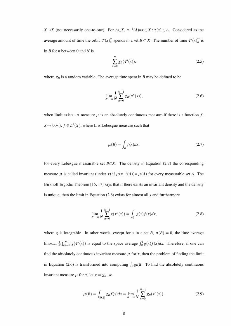
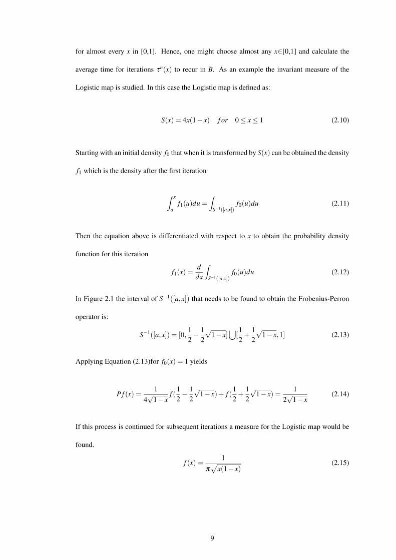
In Figure 2.1 the interval of S−1([a,x]) that needs to be found to obtain the Frobenius-Perron

operator is:

S−1([a,x]) = [0,12− 1

2

√1− x]

⋃[12

+12

√1− x,1] (2.13)

Applying Equation (2.13)for f0(x) = 1 yields

P f (x) =1

4√

1− xf (

12− 1

2

√1− x)+ f (

12

+12

√1− x) =

12√

1− x(2.14)

If this process is continued for subsequent iterations a measure for the Logistic map would be

found.

f (x) =1

π√

x(1− x)(2.15)

9

Figure 2.1: Logistic map transformation.

2.4 Frobenius-Perron Operator

The Frobenius-Perron (F-P) operator is a powerful tool to study invariant measures [16]. Let

us suppose we have a random variable X on [0,1] with

Prob{X ∈ A}=∫

Af dL

where L is Lebesgue measure. We would like to know the probability that X is in A after being

transformed by τ . Thus we write,

Prob{τ(X) ∈ A}= Prob{X ∈ τ−1(A)}=

∫τ−1(A)

f dm.

Furthermore, we would like to know if there exists a function φ such that

Prob{τ(X) ∈ A}=∫

AφdL

10

such a function φ will obviously depend on f and τ . We refer to it as the F-P Operator acting

on f . Let τ:[0,1]→[0,1] be measurable transformation such that m(τ−1(A))=0 if m(A)=0 for A

a measurable subset of [0,1], and define a measure µ where

µ(A) =∫

τ−1(A)f dL

where f ∈L1[0,1] and A is an arbitrary measurable set. It can be seen that L(A)= 0→m(τ−1)(A)=

0→µ(A) = 0, that is µ � m. Then by Radon-Nikodym Theorem [16] there exists φ ∈ L1[0,1]

such that for all measurable sets A.

µ(A) =∫

AφdL

and φ is unique. The F-P operator for τ is defined by setting Pτ f = φ [16]. Thus, for all

measurable sets A⊂ [0,1] ∫A

Pτ f dm =∫

τ−1(A)f dm

from which it follows that ∫ X

0Pτ f dm =

∫τ−1([0,1])

f dm

and so

Pτ f (x) =ddx

∫τ−1([0,1])

f dm.

2.5 Ergodic Theory

Ergodic theory of chaotic systems deals with the statistical properties of trajectories of dynam-

ical systems [15, 17]. Many simple dynamical systems are found to be chaotic, which implies

that long-term predictions are almost impossible from initial observation with limited accu-

racy. However, many chaotic systems are ergodic and ergodic theory can be invoked to make

11

predictions about the average behavior. As was the case with equilibrium statistical mechanics,

this technical difficulty can be overcome by making use of the ergodic hypothesis, which states

that the time average of any sensible function of the phase space variables will be equal to the

ensemble average of this function, with the understanding that the ensemble average must be

taken with respect to the proper stationary, invariant equilibrium measure, µ . In other words,

it can be assume that the systems considered in this thesis will always satisfy the following

condition

limt→∞

1t

∫ t

0dtG( ~Γ(τ)) =

∫d ~Γρ(~Γ)G(~Γ) =

∫µ(d~Γ)G(~Γ), (2.16)

where G is a given function of the phase space variables, corresponding to a physical observ-

able. This definition also is equivalent to the statement that the trajectories in phase space

will spend equal amounts of time in regions of equal volume. Of course, the mathematical

proof that most physical systems are actually ergodic is a formidable task which has seldom

been achieved, even for systems in which experimental observation and computations using

ensemble averages are in excellent agreement.

2.6 Lyapunov Exponent

Lyapunov exponent is another important quantity in nonlinear dynamics. It describes how fast

two adjacent trajectories leave each other in phase space. A measure of the chaotic behavior

of an iterated map is given by the Lyapunov exponent [17, 18]. Specifically, the Lyapunov

Exponent λ (x0) is a measure of the average rate of divergence:

λ (x0) = limn→∞

n−1

∑i=0| dxn+1(xi)

dxi| . (2.17)

In general, the number of Lyapunov exponents (including those which are zero, corresponding

to directions in phase space such that trajectories which follow these directions always remain

12

at a constant separation from each other) will equal the dimensions of the phase space. The

positive exponents correspond to directions in which points stretch out or separate, while the

negative exponents correspond to directions in which point’s contract or approach each other.

In the case where λ (x0) is positive it can be said that the iterated map has a chaotic behavior.

Experimental results for Lyapunov exponent for the chaotic maps [9, 15] are indicated in Ta-

ble 2.1. Also, the plot of Lyapunov exponent for Logistic map is shown in Figure 2.2.

Table 2.1: Lyapunov exponents of chaotic maps

Chaotic Maps λ

Logistic Map 0.69128Tent Map 0.69315

Quadratic Map 0.66122Bernoulli Map 0.70155

Figure 2.2: Lyapunov exponent of Logistic map

13

2.7 Kolmogorov-Sinai Entropy

There is another dynamical quantity which will be of great interest to us, called the K-S entropy,

or hKS for short [19]. This quantity measures the rate at which information can be gained about

the initial configuration of the system [17]. To see how this works, we can imagine that we

have a restricted resolution of our phase space, and it cannot be seen on scales finer than some

small “cubical” region of side ε . At the beginning it is known that our system is represented

by a phase space point contained somewhere inside this small volume element, but cannot say

more than that due to the resolution problem. As this small volume element evolves in time,

it can be seen that its sides will stretch exponentially in time, to lengths of order εeλit where

λi is just one of the positive Lyapunov exponents corresponding to a given direction. If the

whole phase space is partitioned into little cubical regions of side ε , it can be seen in which of

these small regions the system happens to repeat after evolving for a time t. Given that it can

be known the dynamics obeyed by the system, they can be run backwards and thus infer where

this region came from in the original volume, and thus learn more about the initial location of

the system in phase space. It has been shown by Pesin that there is a simple relation between

the positive Lyapunov exponents of a system and its K-S entropy, given by

hKS = ∑λi>0

λi, (2.18)

and this relation, called Pesin’s Theorem, will prove to be quite useful in our study. In partic-

ular, it can be guarantee that a system is chaotic if it has a positive K-S entropy, and for this

reason, the K-S entropy will play a key role in our subsequent investigations.

14

2.8 Fractal Dimension

The Lyapunov exponent λ emphasizes the time-dependent aspects of the chaotic sequence. The

fractal dimension D is another method of quantifying chaos, focusing on the geometric aspects

of chaos [20]. D is a non-integer quantity that can be interpreted as the degree of irregularity of

the signal and is related to the active degrees of freedom, which is denoted by F . Normally D <

F and as a consequence, D helps us to determine how many variables are needed to model the

dynamics of a chaotic system. However, the fractal dimension D is not uniquely defined [21].

Actually, there exist a number of dimensions that can be used (Similarity, Minkowski, Gyration,

Hausdorff, Correlation and Variance) [20, 21].

2.9 Bifurcation

A non-linear dynamical system can behave differently depending on the system’s parameter

values. Different behaviors include periodic, quasiperiodic and chaotic regimes. A system

transitions from one type of behavior to another depends on the value of a set of important

system parameters. These regime transitions occur via a bifurcation process; the parameters

responsible for these regime changes are called bifurcation parameters. The complete dynamic

evolution of a system can be represented by a bifurcation diagram. The bifurcation diagram of

a one-dimensional discrete-time chaotic map is obtained by setting one of the map parameters

to a fixed value and varying a second parameter over a prescribed range. Figure 2.3 shows the

bifurcation diagram of Logistic map.

2.10 Attractors

In general, there are a conservative and a dissipative systems in dynamical systems. However,

in practice, most dynamics is energy dissipative systems which are characterized by contracting

15

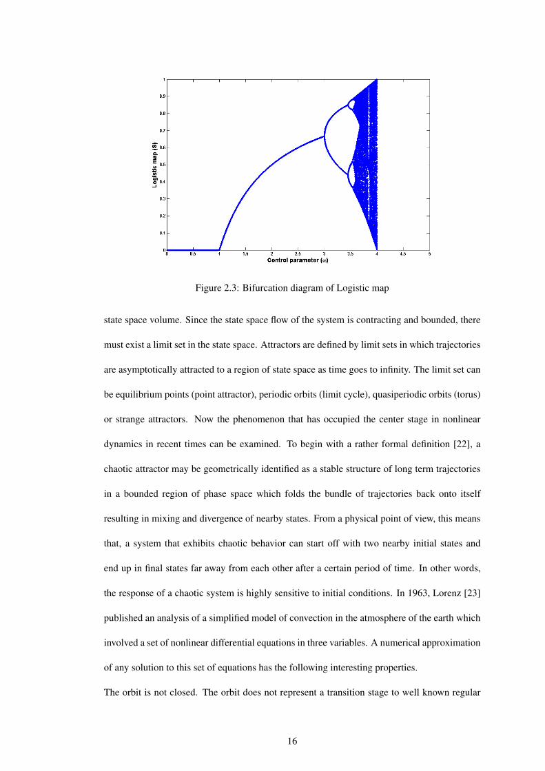
Figure 2.3: Bifurcation diagram of Logistic map

state space volume. Since the state space flow of the system is contracting and bounded, there

must exist a limit set in the state space. Attractors are defined by limit sets in which trajectories

are asymptotically attracted to a region of state space as time goes to infinity. The limit set can

be equilibrium points (point attractor), periodic orbits (limit cycle), quasiperiodic orbits (torus)

or strange attractors. Now the phenomenon that has occupied the center stage in nonlinear

dynamics in recent times can be examined. To begin with a rather formal definition [22], a

chaotic attractor may be geometrically identified as a stable structure of long term trajectories

in a bounded region of phase space which folds the bundle of trajectories back onto itself

resulting in mixing and divergence of nearby states. From a physical point of view, this means

that, a system that exhibits chaotic behavior can start off with two nearby initial states and

end up in final states far away from each other after a certain period of time. In other words,

the response of a chaotic system is highly sensitive to initial conditions. In 1963, Lorenz [23]

published an analysis of a simplified model of convection in the atmosphere of the earth which

involved a set of nonlinear differential equations in three variables. A numerical approximation

of any solution to this set of equations has the following interesting properties.

The orbit is not closed. The orbit does not represent a transition stage to well known regular

16

behavior, for some open regions of parameter space. The orbits with different initial conditions

possess qualitative similarity in the sense that they are bounded within a certain region of phase

space. The system is deterministic. That is, if one were to start from identical initial conditions

one would recover identical orbits. The orbit and the intricate geometrical structure it creates

depend on the initial conditions in a very sensitive way. Thus, a slight perturbation of the initial

conditions produces a very different picture.

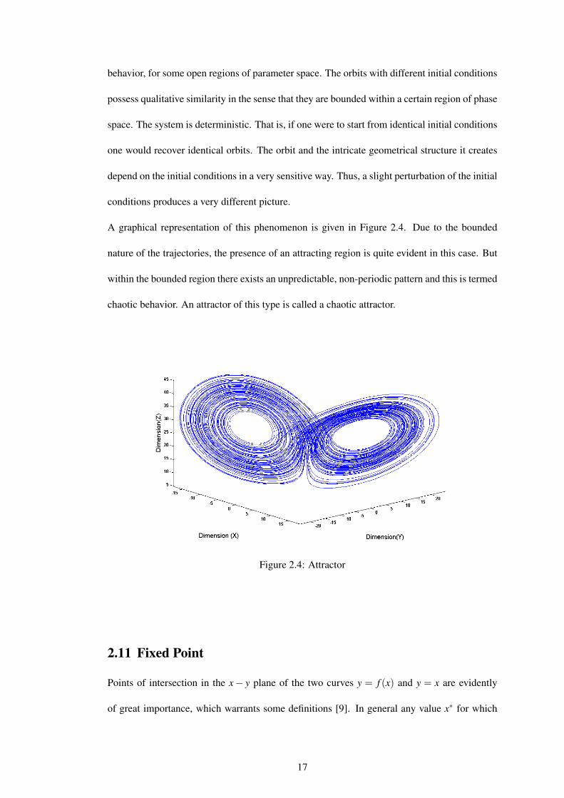
A graphical representation of this phenomenon is given in Figure 2.4. Due to the bounded

nature of the trajectories, the presence of an attracting region is quite evident in this case. But

within the bounded region there exists an unpredictable, non-periodic pattern and this is termed

chaotic behavior. An attractor of this type is called a chaotic attractor.

Figure 2.4: Attractor

2.11 Fixed Point

Points of intersection in the x− y plane of the two curves y = f (x) and y = x are evidently

of great importance, which warrants some definitions [9]. In general any value x∗ for which

17

f (x∗) = x∗ is called a fixed point of f . A fixed point x∗ is stable if it belongs to an interval

I = (a,b), such that for any x0 in I.

• A stable fixed point will also be called an attractor, an unstable fixed point a repeller.

• A fixed point may also be stable in some weaker sense.

2.12 Chaotic Maps

The time behavior of a deterministic system is said to be chaotic when this behavior is aperiodic

and apparently random [19]. Chaotic systems can be mathematically modeled by differential

equations or in the case of discrete systems by difference equations. A solution of a difference

equation is regarded as a sequence of iterations of some initial point under the mapping [24].

Three descriptors are needed to characterize a chaotic system: the time evolution equations, the

values of the parameters describing the systems, and the initial conditions. In some instances,

the dynamics of one-dimensional chaotic systems can be mathematically modeled by chaotic

maps [21]. To have a better understanding of one-dimensional iterated maps, x can be defined

as an independent variable and f (x) can be defined as the iterated map function. Usually an

iterated map depends on certain parameters which may not be shown explicitly. The iteration

begins with an initial value x0, the trajectory of the map is generated by the application of

the map function f (x) [21]. So in general, a chaotic map can be defined by a mathematical

transformation defined as

(n+1) = f (x(n)) (2.19)

An implementation of this mathematical transformation is an iteration of the map.

18

CHAPTER 3

ONE-PARAMETER FAMILIES OF CHAOTIC MAPS

3.1 One-parameter families of chaotic maps

The one-parameter families of chaotic maps of the interval [0,1] with an invariant measure are

defined as the ratio of polynomials of degree N [1, 8, 25]:

Φ(1,2)N (x,α) =

α2F1+(α2−1)F

, (3.1)

F is a substitute for Chebyshev polynomial of type one TN(x) for Φ(1)N (x,α) and Chebyshev

polynomial of type two UN(x) for Φ(2)N (x,α). As an example some of these maps are given

below :

Φ(1)2 =

α2(2x−1)2

4x(1− x)+α2(2x−1)2 , (3.2)

Φ(2)2 =

4α2x(1− x)1+4(α2−1)x(1− x)

, (3.3)

Φ(1)3 = Φ

(2)3 =

α2x(4x−3)2

α2x(4x−3)2 +(1− x)(4x−1)2 , (3.4)

Φ(1)4 =

α2(1−8x(1− x))2

α2(1−8x(1− x))2 +16x(1− x)(1−2x)2 , (3.5)

Φ(2)4 =

16α2x(1− x)(1−2x)2

(1−8x+8x2)2 +16α2x(1− x)(1−2x)2 , (3.6)

Φ(1)5 = Φ

(2)5 =

α2x(16x2−20x+5)2

α2x(16x2−20x+5)2 +(1− x)(16x2− (2x−1)). (3.7)

where the map Φ(2)2 (x,α) reduces to Logistic map if α = 1.

Invariant measure for one-parameter families of chaotic maps is calculated and presented

19

in Appendix A.

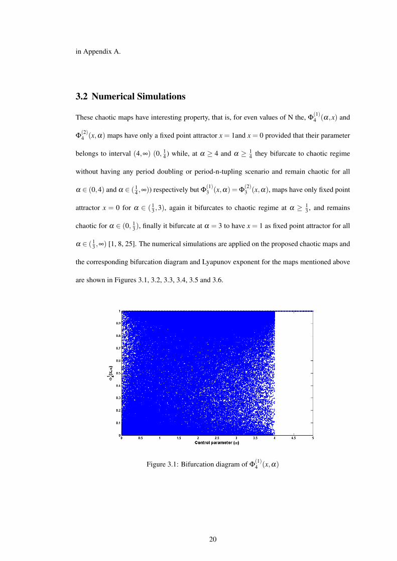
3.2 Numerical Simulations

These chaotic maps have interesting property, that is, for even values of N the, Φ(1)4 (α,x) and

Φ(2)4 (x,α) maps have only a fixed point attractor x = 1and x = 0 provided that their parameter

belongs to interval (4,∞) (0, 14 ) while, at α ≥ 4 and α ≥ 1

4 they bifurcate to chaotic regime

without having any period doubling or period-n-tupling scenario and remain chaotic for all

α ∈ (0,4) and α ∈ (14 ,∞)) respectively but Φ

(1)3 (x,α) = Φ

(2)3 (x,α), maps have only fixed point

attractor x = 0 for α ∈ (13 ,3), again it bifurcates to chaotic regime at α ≥ 1

3 , and remains

chaotic for α ∈ (0, 13), finally it bifurcate at α = 3 to have x = 1 as fixed point attractor for all

α ∈ (13 ,∞) [1, 8, 25]. The numerical simulations are applied on the proposed chaotic maps and

the corresponding bifurcation diagram and Lyapunov exponent for the maps mentioned above

are shown in Figures 3.1, 3.2, 3.3, 3.4, 3.5 and 3.6.

Figure 3.1: Bifurcation diagram of Φ(1)4 (x,α)

20

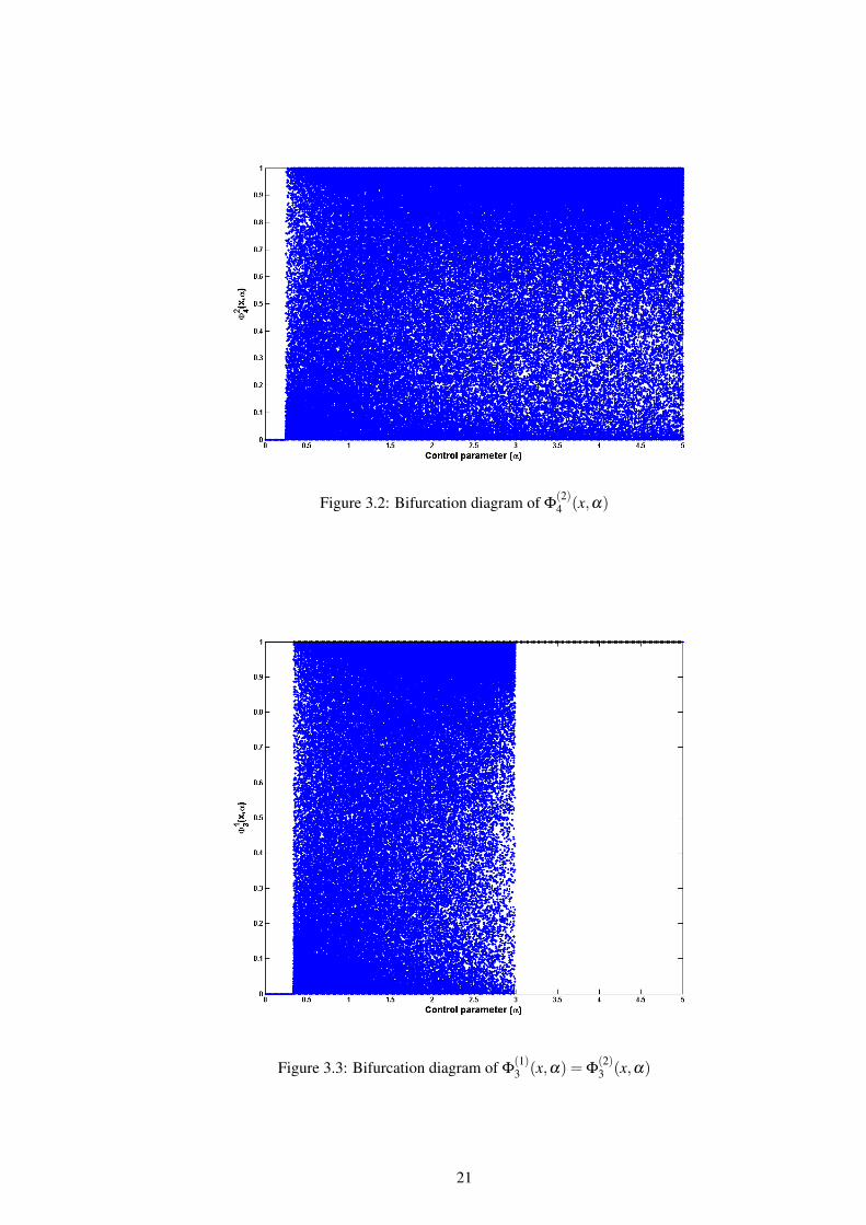
Figure 3.2: Bifurcation diagram of Φ(2)4 (x,α)

Figure 3.3: Bifurcation diagram of Φ(1)3 (x,α) = Φ

(2)3 (x,α)

21

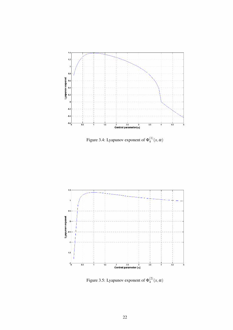
Figure 3.4: Lyapunov exponent of Φ(1)4 (x,α)

Figure 3.5: Lyapunov exponent of Φ(2)4 (x,α)

22

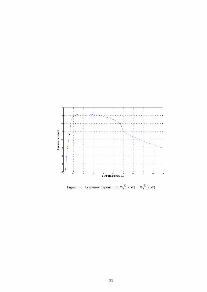
Figure 3.6: Lyapunov exponent of Φ(1)3 (x,α) = Φ

(2)3 (x,α)

23

CHAPTER 4

HIERARCHY OF 2D PIECEWISE NONLINEARCHAOTIC MAPS

4.1 Two Dimensional Piecewise Nonlinear Chaotic Maps

The most popular discrete time map that has been used in cryptography is Logistic map. Logis-

tic map is generalized to a hierarchy of one-parameter families of maps with ergodic behavior,

in the interval [0,1]. The hierarchy can be defined as (see [1], for the details):

Φ(1,2)N (x,α) =

α2TN(√

x)1+(α2−1)TN(

√x)

, (4.1)

The maps ΦN(α,x), are (N−1)-nodal maps, that is, they have (N−1) critical points in unit in-

terval [0,1] [18] and they have only single period one stable fixed points or they are ergodic [1].

As an example one of these maps are given below:

Φ(2)2 =

4α2x(1− x)1+4(α2−1)x(1− x)

, (4.2)

Now using the pieces of these one-dimensional maps, a new hierarchy of ergodic two-

dimensional piecewise nonlinear chaotic maps is constructed and which can be defined as:

ΦN,N1,N2,..,NN (x,α,y,b1,b2, ...,bN)

xn+1 = ΦN(xn,α) = α2(TN(√

xn))2

1+(α2−1)(TN(√

xn)2)

xn ∈ [0, x1]

yn+1 = ΦN1(yn,b1) = b21(TN1 (

√yn))2

1+(b21−1)(TN1 (

√yn)2)

24