A class of local classical solutions for the

one-dimensional Perona-Malik equation

Marina Ghisi

Universita degli Studi di Pisa

Dipartimento di Matematica “Leonida Tonelli”

Largo Bruno Pontecorvo 5, 56127 PISA (Italy)

e-mail: ghisi@dm.unipi.it

Massimo Gobbino

Universita degli Studi di Pisa

Dipartimento di Matematica Applicata “Ulisse Dini”

Via Filippo Buonarroti 1c, 56127 PISA (Italy)

e-mail: m.gobbino@dma.unipi.it

November 13, 2006

Abstract

We consider the Cauchy problem for the one-dimensional Perona-Malik equation

ut =1 − u2

x

(1 + u2x)

2uxx

in the interval [−1, 1], with homogeneous Neumann boundary conditions.We prove that the set of initial data for which this equation has a local-in-time

classical solution u : [−1, 1]×[0, T ] → R is dense in C1([−1, 1]). Here “classical solution”means that u, ut, ux and uxx are continuous functions in [−1, 1] × [0, T ].

Mathematics Subject Classification 2000 (MSC2000): 35A07, 35B65, 35K65.

Key words: Perona-Malik equation, classical solution, forward-backward parabolicequation, anisotropic diffusion, supersolutions, comparison principles.

1 Introduction

In this paper we consider the initial boundary value problem

ut =1 − u2

x

(1 + u2x)

2uxx in [−1, 1] × [0, T ], (1.1)

ux(−1, t) = ux(1, t) = 0 ∀t ∈ [0, T ], (1.2)

u(x, 0) = u0(x) ∀x ∈ [−1, 1]. (1.3)

Since we are interested in classical solutions, we require that (1.1) and (1.2) are sat-isfied also for t = 0. In particular we always consider initial conditions u0 ∈ C2([−1, 1])and such that u0x(−1) = u0x(1) = 0.

Formally, equation (1.1) is an instance of the usual parabolic PDE in divergenceform ut = (ϕ′(ux))x = ϕ′′(ux)uxx, corresponding to ϕ(σ) = 2−1 log(1 + σ2). The mainfeature is that ϕ(σ) is convex for |σ| < 1 and concave for |σ| > 1. This implies that(1.1) is a forward-parabolic PDE where |ux| < 1 (the forward or subcritical region), anda backward-parabolic PDE where |ux| > 1 (the backward or supercritical region).

Equation (1.1) is the one-dimensional version of the diffusion process introduced in[15] in the context of image processing. Numerical computations seem to show that thisequation produces the desired denoising effect on the initial condition u0 despite of theexpected ill posedness: this is usually referred as “the Perona-Malik paradox”.

The mathematical understanding of this phenomenology is still quite poor. Theresearch has developed along three main lines: finding a suitable notion of weak solutionconsistent with experiments [4, 7, 9, 13, 16, 17], proving a priori estimates on classicalsolutions yielding existence or non existence results [8, 9, 12], extending some one-dimensional results to higher dimension [5, 9].

In this paper we focus on classical solutions, namely solutions with one derivativewith respect to time and two derivatives in the space variable. The following results areby now well established in the literature.

• If u0(x) is subcritical, i.e. |u0x(x)| < 1 for all x ∈ [−1, 1], then (1.1), (1.2), (1.3)has a global (defined for every t ≥ 0) classical solution which remains subcriticalfor all times [12].

• If u0(x) is transcritical, i.e. ϕ′′(u0x) changes its sign in [−1, 1], then classical solu-tions, if they exist, cannot be global [12, 10]. In particular in [10] it is proved thatfor a transcritical solution we have that necessarily

T ≤ 4

∫ 1

−1

log(1 + u20x(x)) dx. (1.4)

1

• Let us assume that a classical local solution exists for some transcritical u0(x),and let us consider any closed interval contained in the supercritical region of u0.As remarked in [13], in this interval u0 is the trace at t = 0 of the solution ofa backward strictly parabolic equation. Therefore the standard regularity theoryprovides severe restrictions on u0. For example, a necessary (but by no meanssufficient) condition is that u0 is of class C∞ in its supercritical region.

To our knowledge, up to now no example of local classical solution with a tran-scritical u0 had been shown. We refer the reader to [12, Section 6] for a discussionon some apparently inconclusive approaches to local solutions, including higher orderregularization, vanishing viscosity, power series expansions.

Some signs made people even skeptical about their existence. From the analyticalpoint of view it was proved in [10] that the trivial stationary solutions u(x, t) = ax+b arethe unique classical solutions of (1.1) defined for every (x, t) ∈ R

2. From the numericalpoint of view, experiments on some regularizations of (1.1) showed a rapid formationof microstructures with a drastic reduction of the energy in the backward region [3].This phenomenon, usually referred as staircasing [13] or fibrillation [6], happens in atime scale which vanishes with the regularization parameter [3]. After the formationof microstructures the evolution in the backward region slows down and the dynamicis governed by the forward region. This may lead to suspect that in the limit theevolution of any transcritical initial condition should exhibit the instantaneous formationof discontinuities in ux and maybe also in u.

We show that this is not always the case, because some local classical transcriticalsolutions do exist. We have indeed the following existence result (throughout this paperC2,1 denotes the usual parabolic space of functions u(x, t) such that u, ut, ux and uxx

are continuous functions).

Theorem 1.1 Let R ⊆ C1([−1, 1]) be the set of initial data u0(x) for which there existsT > 0 and u ∈ C2,1([−1, 1] × [0, T ]) satisfying (1.1), (1.2), and (1.3).

Then R is dense in C1([−1, 1]).

The same is true for all equations ut = ϕ′′(ux)uxx with ϕ ∈ C∞(R) (this regularityrequirement can probably be weakened) and such that the set σ ∈ R : ϕ′′(σ) = 0 hasno accumulation points.

Note that in Theorem 1.1, in order to obtain density, we are forced to admit thatthe life span T of the solution depends on the initial condition. This may seem toorestrictive, but it is not. Indeed there are transcritical data for which the right handside of (1.4) is arbitrarily small: it follows that the set of initial data for which a classicalsolution exists at least on a fixed time interval [0, T ] cannot be dense in C1([−1, 1]).

Our proof doesn’t characterize all initial data for which a local solution exists (andwe suspect that a non-tautological characterization doesn’t exist). We only exhibit a

2

quite special class of such data, which however turns out to be dense in C1([−1, 1]),hence a fortiori in C0([−1, 1]) or in L2((−1, 1)). On the other hand [13] shows thatnothing more than density can be expected.

The rough idea of our construction is the following. Let us take any v0 ∈ C∞([−1, 1])such that |v0x(x)| = 1 in a finite number of points. Let I+ and I− be the subcritical andthe supercritical region of v0, respectively (both I+ and I− are finite unions of intervals).Given T > 0 we prove (Theorem 2.1) that there exists a solution u of (1.1), (1.2) whichat t = 0 coincides with v0 in I+ and at t = T coincides with v0 in I−. This means that v0

acts as an initial condition in I+ and as a final condition in I−. In order to construct sucha solution we solve a separate problem in any connected component of I+ and I−: thissub-problem is always well posed because it is either a (degenerate) forward parabolicproblem with an initial condition or a (degenerate) backward parabolic problem with afinal condition. The main point is that the solutions of these sub-problems glue togetherin a C2,1 way provided that T is small enough and v0xx(x) = 0 whenever |v0x(x)| = 1.The required estimates are proved in Theorem 2.2 and Theorem 2.3 using standardenergy estimates in the interior and suitable subsolutions and supersolutions to controlthe behavior near the boundary.

If we now define u0(x) as u(x, 0), we have found an initial condition for which (1.1),(1.2), (1.3) has a local solution, hence the set R is nonempty. Notice that u0 coincideswith v0 in I+, while in I− it is the trace at t = 0 of a solution of a backward problem,as required by [13].

Finally, if we choose T small enough it is clear that u0 is as close as we want to v0

in the C2([−1, 1]) topology. Since the set of admissible v0 (see Theorem 2.1) is in turndense in C1([−1, 1]), we easily conclude that R is dense in C1([−1, 1]).

We conclude by speculating on some consequences of Theorem 1.1.From the analytical point of view, classical solutions are naturally welcome. They

also give a new light to a priori estimates on smooth solutions [9, 12]. Up to now indeedthere was a diffuse suspect they were likely to be vacuous in the transcritical case.

From the numerical point of view things may be different. On one hand classicalsolutions are not a solution of the Perona-Malik paradox, since there is no reason forthem to be stable or to exist but for special classes of smooth initial data (while agood theory is expected for BV data). On the other hand, it is easy to see that classicalsolutions must be kept into account by any reasonable stable theory. We state it formallyin the case of the fourth order regularization (Remark 2.4), but analogous statementsare true for the semi-discrete scheme and maybe also for several other approximationsof (1.1). The rough idea is the following: our classical solutions can be obtained aslimits in the C2,1 topology of solutions of the regularized problems up to adding a smallperturbation which vanishes in the C0 norm with the regularization parameter.

This proves that any stable theory allowing perturbations vanishing in C0 and con-vergence of solutions in C2,1 cannot neglect the dynamics in supercritical regions, as on

3

the contrary it seemed to be suggested by numerical experiments and some analyticalresults on simpler models [4]. For this reason, a solution of the Perona-Malik paradoxseems now even further away.

Remark 2.4 can of course be compared with [9], where it is shown that any theoryallowing perturbations vanishing in L2 and uniform convergence of solutions contains thestationary solution for every initial datum in BV , and with [16] (see also the pioneeringpaper [11]) where it is shown that any theory allowing perturbations vanishing in W−1,∞

and uniform convergence of solutions contains plenty of exotic solutions even for smoothsubcritical data.

The plan of this paper is the following. In section 2 we state Theorem 2.1 and weshow how its proof reduces to the proof of Theorem 2.2 and Theorem 2.3. In section 3we give the details of the proofs.

2 Statements

As we have seen in the introduction, Theorem 1.1 is a straightforward consequence ofthe following result, where we prove well posedness for (1.1), (1.2) with a mixture ofinitial and final conditions.

Theorem 2.1 Let n ∈ N, and let −1 = a0 < a1 < . . . < a2n < a2n+1 = 1. Let usconsider the open sets

I− :=n⋃

i=1

(a2i−1, a2i), I+ :=n⋃

i=0

(a2i, a2i+1).

Let v0 ∈ C∞([−1, 1]) be a function such that

(i) |v0x(x)| < 1 for every x ∈ I+ and |v0x(x)| > 1 for every x ∈ I−;

(ii) v0xx(x) = 0 for every x ∈ a1, . . . , a2n;

(iii) all derivatives of v0 with odd order are zero at x = −1 and x = 1.

Then for every T > 0 small enough there exists u ∈ C2,1([−1, 1] × [0, T ]) satisfying(1.1), (1.2), and

u(x, 0) = v0(x) ∀x ∈ I+;

u(x, T ) = v0(x) ∀x ∈ I−;

u(x, t) = v0(x) ∀(x, t) ∈ a1, . . . , a2n × [0, T ].

Moreover

|ux(x, t)| < 1 in I+ × [0, T ] and |ux(x, t)| > 1 in I− × [0, T ]; (2.1)

4

ux(x, t) = v0x(x) ∀(x, t) ∈ a1, . . . , a2n × [0, T ]. (2.2)

uxx(x, t) = 0 ∀(x, t) ∈ a1, . . . , a2n × [0, T ]. (2.3)

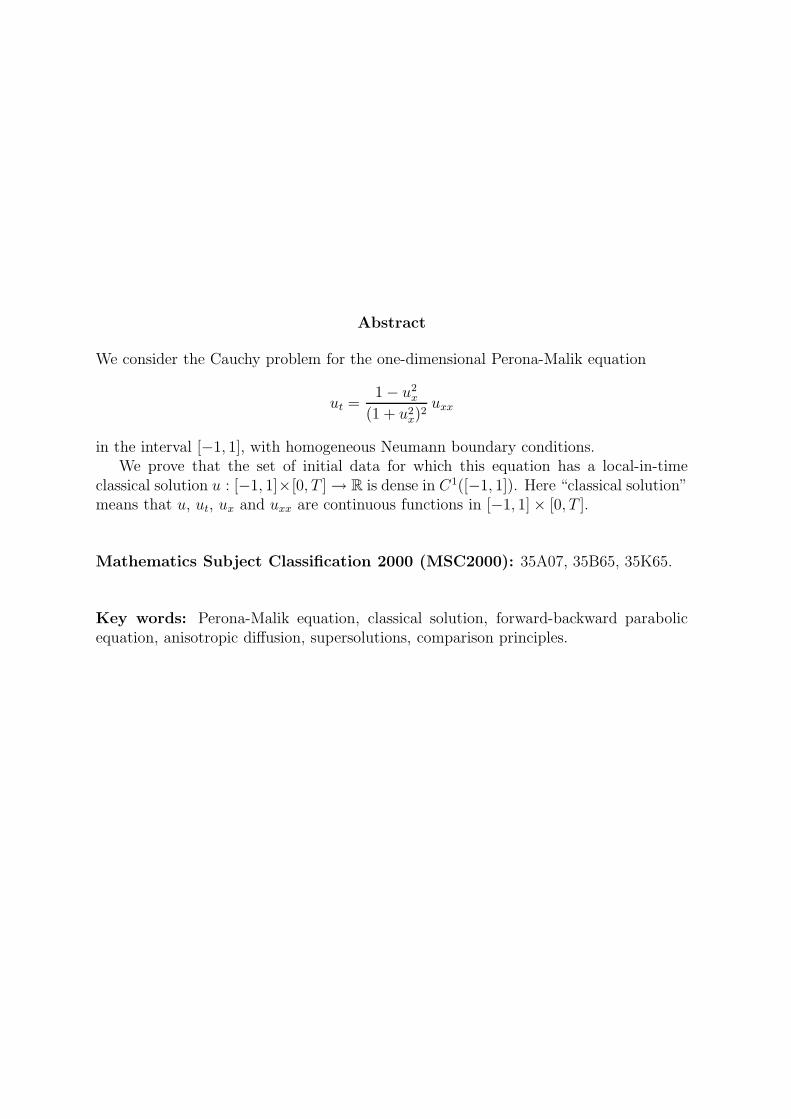
The situation described in Theorem 2.1 is represented in Figure 1 in the particularcase n = 2. The function v0 is prescribed as an initial condition in the lower horizontalthick segments, as a final condition in the upper horizontal thick segments, and as aDirichlet condition in the vertical thick segments. We have Neumann boundary condi-tions in the vertical dashed segments. The shaded regions represent the supercriticalzone I− × [0, T ].

In the general case the rectangle [−1, 1] × [0, T ] is divided into 2n + 1 subrectan-gles. Now we solve (1.1) separately in each subrectangle with the appropriate boundaryconditions. We end up with problems of three types.

• D-D-forward problems. In rectangles (a2i, a2i+1) × [0, T ] (i = 1, . . . , n − 1) (R3in the picture) we have a forward parabolic equation with an initial datum andDirichlet boundary conditions.

• D-D-backward problems. In rectangles (a2i−1, a2i) × [0, T ] (i = 1, . . . , n) (R2 andR4 in the picture) we have a backward parabolic equation with a final datum andDirichlet boundary conditions. These problems can be reduced to D-D-forwardproblems just by reversing the time.

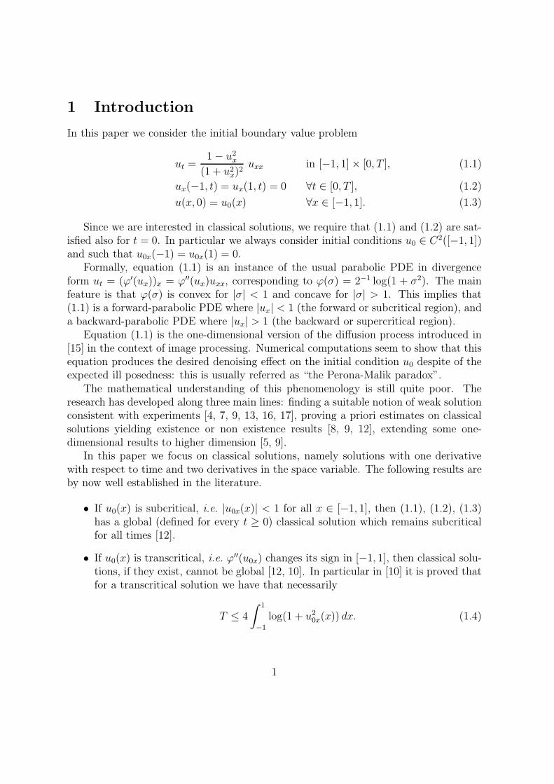
• N-D-forward problems. In the lateral rectangles (−1, a1)×[0, T ] and (a2n, 1)×[0, T ](R1 and R5 in the picture) we have a forward parabolic equation with an initialdatum, a Dirichlet boundary condition in one of the endpoints of the space interval,and a homogeneous Neumann boundary condition in the other endpoint. Thisproblems can be reduced to D-D-forward problems with a standard reflectionargument. For example in the case of the rectangle on the left we can definea′1 as the symmetric of a1 with respect to −1 (see Figure 2), and extend v0 to theinterval [a′1, a1] in such a way that v0(−1 − x) = v0(−1 + x). By assumption (iii)in Theorem 2.1 the extension is still of class C∞.

The solution of the symmetrized problem is clearly symmetric with respect tox = −1. It follows that its restriction to [−1, a1] × [0, T ] satisfies the homogenousNeumann boundary condition at x = −1.

It is clear that for every choice of T > 0 the solutions found in the subrectanglesglue together in a C0 way. The main point is proving that the glueing is actually ofclass C2,1. This is where the smallness of T and assumption (ii) in Theorem 2.1 playa fundamental role. Under such assumptions indeed it turns out that not only u(x, t)coincides with v0(x) for x ∈ a1, . . . , a2n, but also ux(x, t) and uxx(x, t) coincide withv0x(x) and v0xx(x), respectively, at the same points. In a certain sense conditions (2.2)

5

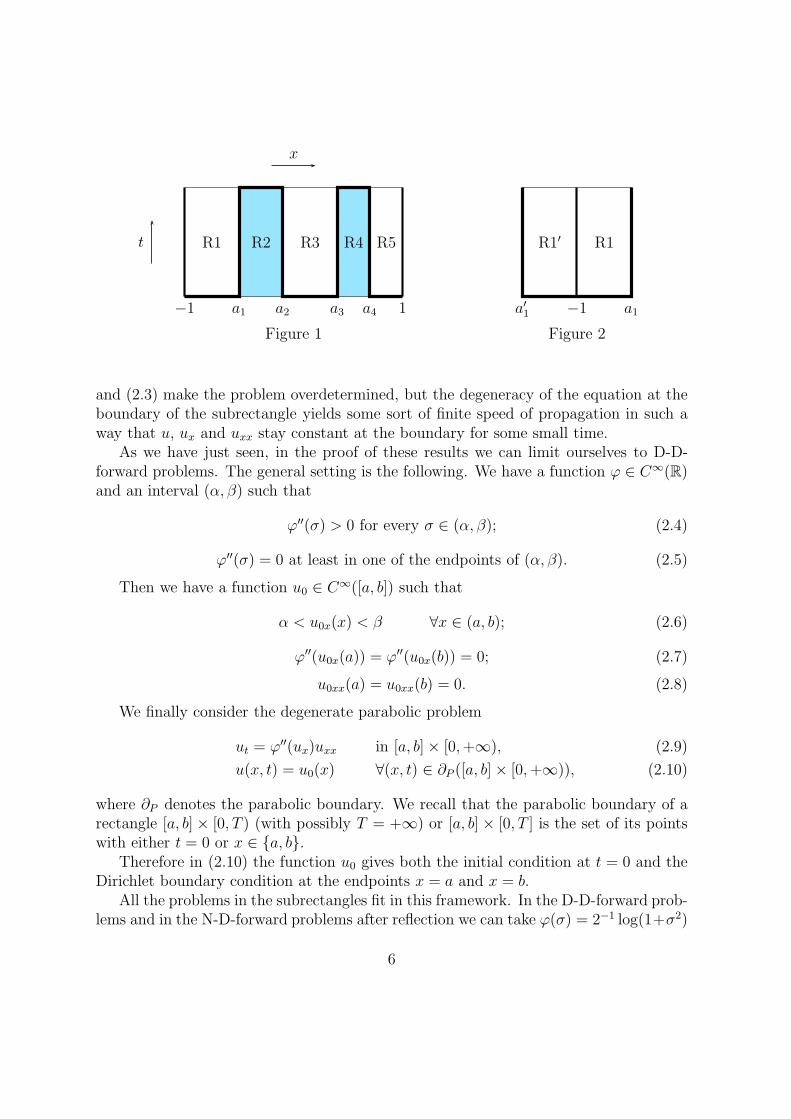
−1 a1 a2 a3 a4 1

R1 R2 R3 R4 R5t

x

Figure 1

a1−1a′1

R1′ R1

Figure 2

and (2.3) make the problem overdetermined, but the degeneracy of the equation at theboundary of the subrectangle yields some sort of finite speed of propagation in such away that u, ux and uxx stay constant at the boundary for some small time.

As we have just seen, in the proof of these results we can limit ourselves to D-D-forward problems. The general setting is the following. We have a function ϕ ∈ C∞(R)and an interval (α, β) such that

ϕ′′(σ) > 0 for every σ ∈ (α, β); (2.4)

ϕ′′(σ) = 0 at least in one of the endpoints of (α, β). (2.5)

Then we have a function u0 ∈ C∞([a, b]) such that

α < u0x(x) < β ∀x ∈ (a, b); (2.6)

ϕ′′(u0x(a)) = ϕ′′(u0x(b)) = 0; (2.7)

u0xx(a) = u0xx(b) = 0. (2.8)

We finally consider the degenerate parabolic problem

ut = ϕ′′(ux)uxx in [a, b] × [0,+∞), (2.9)

u(x, t) = u0(x) ∀(x, t) ∈ ∂P ([a, b] × [0,+∞)), (2.10)

where ∂P denotes the parabolic boundary. We recall that the parabolic boundary of arectangle [a, b] × [0, T ) (with possibly T = +∞) or [a, b] × [0, T ] is the set of its pointswith either t = 0 or x ∈ a, b.

Therefore in (2.10) the function u0 gives both the initial condition at t = 0 and theDirichlet boundary condition at the endpoints x = a and x = b.

All the problems in the subrectangles fit in this framework. In the D-D-forward prob-lems and in the N-D-forward problems after reflection we can take ϕ(σ) = 2−1 log(1+σ2)

6

and (α, β) = (−1, 1). As for D-D-backward problems, after reversing the time we mayassume ϕ(σ) = −2−1 log(1 + σ2) and (α, β) defined as follows: if u0x > 1 in the givensub-interval, then we take α = 1 and β any strict upper bound for u0x; if u0x < −1 inthe given sub-interval, then we take β = −1 and α any strict lower bound for u0x. Inall the cases u0 is either v0 or its extension by reflection in the N-D-forward problems.

Theorem 2.2 Let us assume that ϕ and u0 satisfy (2.4) through (2.8).Then there exists a unique function u ∈ C0([a, b] × [0,+∞)) ∩ C∞((a, b) × [0,+∞))

satisfying (2.9), (2.10), and the estimate

α < ux(x, t) < β ∀(x, t) ∈ (a, b) × [0,+∞). (2.11)

Moreover there exists T0 > 0 such that u ∈ C2,1([a, b] × [0, T0]) and

ux(a, t) = u0x(a), ux(b, t) = u0x(b) ∀t ∈ [0, T0]; (2.12)

uxx(a, t) = uxx(b, t) = 0 ∀t ∈ [0, T0]. (2.13)

Some parts of Theorem 2.2 are probably scattered in the huge porous medium lit-erature. The C2,1 regularity is in any case beyond the optimal regularity for this typeof equations [1, 2], and this is of course due to assumptions (2.7) and (2.8). In orderto take advantage of these assumptions we give a self contained proof of Theorem 2.2,which only relies on the theory of strictly parabolic problems [14].

To this end, given ε > 0, we approximate u0(x) with

uε0(x) :=

u0(x)

1 + ε+ε(α+ β)

2(1 + ε)x. (2.14)

The motivation of this choice is that if α ≤ u0x(x) ≤ β for every x ∈ [a, b], thenthere exists constants αε and βε such that

α < αε ≤ uε0x(x) ≤ βε < β ∀x ∈ [a, b]. (2.15)

Now we consider the following problem

uεt = ϕ′′(uε

x)uεxx in [a, b] × [0,+∞), (2.16)

uε(x, t) = uε0(x) ∀(x, t) ∈ ∂P ([a, b] × [0,+∞)). (2.17)

This problem turns out to be strictly parabolic. The following result collects theestimates that are needed for the proof of Theorem 2.2.

7

Theorem 2.3 Let us assume that ϕ and u0 satisfy (2.4) through (2.8). Let ε > 0, andlet uε

0, αε and βε be defined by (2.14) and (2.15).Then there exists a unique function

uε ∈ C2,1([a, b] × [0,+∞)) ∩ C∞((a, b) × [0,+∞)) ∩ C∞([a, b] × (0,+∞)) (2.18)

satisfying (2.16), (2.17), and

αε ≤ uεx(x, t) ≤ βε ∀(x, t) ∈ (a, b) × [0,+∞), (2.19)

uεxx(x, t) = 0 ∀(x, t) ∈ a, b × [0,+∞). (2.20)

Moreover uε satisfies the following estimates independent on ε.

1. Global estimates on ut. There exists a constant M1 such that

∫ b

a

[uεt (x, t)]

2 dx ≤M1 ∀t ≥ 0, (2.21)

∫ T

0

∫ b

a

ϕ′′(uεx(x, t))[u

εxt(x, t)]

2 dx dt ≤M1 ∀T ≥ 0. (2.22)

2. Uniform strict parabolicity in the interior. For every closed interval [x1, x2] ⊆ (a, b)and every T > 0 there exist constants M2 and M3 such that

α < M2 ≤ uεx(x, t) ≤M3 < β ∀(x, t) ∈ [x1, x2] × [0, T ]. (2.23)

As a consequence, there exists a constant M4 > 0 such that

ϕ′′(uεx(x, t)) ≥ M4 ∀(x, t) ∈ [x1, x2] × [0, T ]. (2.24)

3. Interior estimates. For every closed interval [x1, x2] ⊆ (a, b) and every T > 0 thereexists a constant M5 such that

∫ x2

x1

[uεxt(x, t)]

2 dx ≤ M5 ∀t ∈ [0, T ], (2.25)

∫ T

0

∫ x2

x1

[uεxxt(x, t)]

2 dx dt ≤ M5, (2.26)

|uεxx(x, t)| ≤ M5 ∀(x, t) ∈ [x1, x2] × [0, T ]. (2.27)

4. Uniform vanishing of uεxx at the boundary. There exist constants T0 > 0 and M6

such that

|uεxx(x, t)| ≤ M6(x− a)(b− x) ∀(x, t) ∈ [a, b] × [0, T0]. (2.28)

8

We conclude by remarking that classical solutions cannot be neglected when lookingfor a stable notion of weak solution. We show indeed that they are obtained by fourthorder regularization with a vanishing continuous perturbation.

Remark 2.4 Let u ∈ C2,1([−1, 1] × [0, T ]) be any classical solution of (1.1), (1.2).Then there exist families f ε ⊆ C0([−1, 1]× [0, T ]) and uε ⊆ C2,1([−1, 1]× [0, T ])

such that

uεt = ϕ′′(uε

x)uεxx − εuε

xxxx + f ε(x, t) ∀(x, t) ∈ [−1, 1] × [0, T ], (2.29)

uεx(x, t) = uε

xxx(x, t) = 0 ∀(x, t) ∈ −1, 1 × [0, T ], (2.30)

uε → u in C2,1([−1, 1] × [0, T ]), (2.31)

f ε → 0 in C0([−1, 1] × [0, T ]). (2.32)

We chose fourth order regularizations only because in this framework the result canbe stated without further definitions. An analogous statement holds true for higherorder regularizations and for the semi-discrete scheme considered in [9].

3 Proofs

3.1 Compactness and comparison results

In this section we collect two technical results. They look classical, but we didn’t findthese exact statements in the literature. For this reason in both cases we give a sketchof the proof for the convenience of the reader.

The first one is a compactness result. We recall that C1/2,1/4([a, b] × [0, T ]) is thespace of functions f : [a, b] × [0, T ] → R for which there exists a constant N such that

|f(x1, t1) − f(x2, t2)| ≤ N(

|x1 − x2|1/2 + |t1 − t2|

1/4)

(3.1)

for every x1, x2 in [a, b], and every t1, t2 in [0, T ].

Lemma 3.1 For every ε ∈ (0, ε0) let f ε ∈ C1([a, b] × [0, T ]). Let us assume that thereexists M ∈ R such that

∫ T

0

∫ b

a

[f εt (x, t)]2 dx dt ≤ M ∀ε ∈ (0, ε0), (3.2)

∫ b

a

[f εx(x, t)]2 dx ≤ M ∀t ∈ [0, T ], ∀ε ∈ (0, ε0), (3.3)

|f ε(a, 0)| ≤ M ∀ε ∈ (0, ε0). (3.4)

Then the family f ε is relatively compact in C0([a, b] × [0, T ]) and any limit pointbelongs to C1/2,1/4([a, b] × [0, T ]).

9

Proof. It is enough to prove that any function f satisfying (3.2) and (3.3) satisfiesalso (3.1) with a constant N independent on ε. At this point it is indeed easy toconclude that the family f ε is equicontinuous and equibounded, hence it is compactfor the uniform convergence by the Ascoli-Arzela Theorem.

In order to prove (3.1), let us first remark that we can prove it under the additionalassumption that |t1 − t2| < (b− a)2. Now let us write

|f(x1, t1) − f(x2, t2)| ≤ |f(x1, t1) − f(x2, t1)| + |f(x2, t1) − f(x2, t2)| =: A +B.

By (3.3) and Cauchy-Schwarz inequality we have that

A ≤

∣

∣

∣

∣

∫ x2

x1

fx(x, t1) dx

∣

∣

∣

∣

≤M1/2|x2 − x1|1/2. (3.5)

In order to estimate B, let us set Bδ(x2) = x ∈ [a, b] : |x− x2| < δ. If δ is smallerthan b− a, then δ ≤ |Bδ(x2)| ≤ 2δ. Moreover there exist xδ and yδ in Bδ(x2) such that

1

|Bδ(x2)|

∫

Bδ(x2)

f(x, t1) dx = f(xδ, t1),1

|Bδ(x2)|

∫

Bδ(x2)

f(x, t2) dx = f(yδ, t2).

Now

B ≤ |f(x2, t1) − f(xδ, t1)| + |f(xδ, t1) − f(yδ, t2)| + |f(yδ, t2) − f(x2, t2)|

=: B1 +B2 + B3.

Using (3.3) as we did in (3.5) it is easy to see that B1 ≤M1/2δ1/2 and B3 ≤M1/2δ1/2.Moreover, by (3.2) and Cauchy-Schwarz inequality applied in the rectangle Bδ(x2)×

[t1, t2] (we assume that t1 < t2 without loss of generality) we have that

B2 ≤1

|Bδ(x2)|

∫

Bδ(x2)

|f(x, t1) − f(x, t2)| dx

≤1

|Bδ(x2)|

∫

Bδ(x2)

∫ t2

t1

|ft(x, t)| dx dt

≤1

|Bδ(x2)||Bδ(x2)| · |t2 − t1|

1/2M1/2

≤ M1/2δ−1/2|t2 − t1|1/2.

Putting all together we have that

A +B ≤ M1/2|x2 − x1|1/2 + 2M1/2δ1/2 +M1/2δ−1/2|t2 − t1|

1/2,

and therefore (3.1) follows by setting δ := |t2 − t1|1/2 (which we assumed to be smaller

than b− a). 2

The second result is one of the infinite variants of the comparison principle for fullynonlinear parabolic PDEs.

10

Lemma 3.2 Let Ω ⊆ R2, and let ψ : [a, b]× [0, T ]×Ω×R → R be a continuous function

which is nondecreasing in the last variable, i.e.

ψ(x, t, p, q, r) ≥ ψ(x, t, p, q, s) ∀r ≥ s (3.6)

for all admissible values of x, t, p, q (this condition is usually called weak ellipticity).Let u ∈ C0([a, b] × [0, T ]) ∩ C2,1((a, b) × (0, T ]) be a function such that

(u(x, t), ux(x, t)) ∈ Ω ∀(x, t) ∈ (a, b) × (0, T ], (3.7)

ut = ψ(x, t, u, ux, uxx) in (a, b) × (0, T ]. (3.8)

Let v ∈ C0([a, b] × [0, T ]) ∩ C2,1((a, b) × (0, T ]), and let

VΩ := (x, t) ∈ (a, b) × (0, T ] : (v(x, t), vx(x, t)) ∈ Ω.

Let us assume that

vt > ψ(x, t, v, vx, vxx) ∀(x, t) ∈ VΩ, (3.9)

v(x, t) > u(x, t) ∀(x, t) ∈ ∂P ([a, b] × [0, T ]). (3.10)

Then v(x, t) > u(x, t) for every (x, t) ∈ [a, b] × [0, T ].An analogous statement can be obtained by reversing the inequality signs in (3.9),

(3.10), and in the conclusion.

Proof. Let z(x, t) := v(x, t) − u(x, t). We claim that z(x, t) > 0 for every (x, t) ∈[a, b] × [0, T ]. Let us assume by contradiction that this is not the case, and let

t0 := inft ∈ [0, T ] : z(x, t) ≤ 0 for some x ∈ [a, b].

Then it is easy to see that there exists x0 ∈ [a, b] such that z(x0, t0) = 0, hencev(x0, t0) = u(x0, t0) =: p0. From (3.10) and the continuity of z it follows that t0 > 0 andx0 ∈ (a, b). Therefore zt(x0, t0) ≤ 0, zx(x0, t0) = 0, hence ux(x0, t0) = vx(x0, t0) =: q0,and zxx(x0, t0) ≥ 0, hence vxx(x0, t0) ≥ uxx(x0, t0).

In particular (x0, t0) ∈ VΩ, hence by (3.9), (3.8), and the weak ellipticity (3.6) of ψwe have that

0 ≥ zt(x0, t0) = vt(x0, t0) − ut(x0, t0)

> ψ(x0, t0, p0, q0, vxx(x0, t0)) − ψ(x0, t0, p0, q0, uxx(x0, t0)) ≥ 0,

which is absurd. 2

11

3.2 Proof of Theorem 2.3

Global existence and maximum principle for ux In order to prove existenceof a global solution of (2.16), (2.17) we take a function ϕε ∈ C∞(R) which coincideswith ϕ in the interval (αε, βε) and such that ϕ′′

ε(σ) ≥ ν > 0 for every σ ∈ R. Problem(2.16), (2.17), with ϕε instead of ϕ, is strictly parabolic. By well knows results (see forexample [14]) it admits a unique global solution with the regularity stated in (2.18).

Since the initial condition uε0 satisfies (2.15), the classical maximum principle for uε

x

implies that this solution satisfies (2.19), and in particular it is also a solution of (2.16),(2.17) with the original ϕ. Finally, since the equation is strictly parabolic, (2.20) isequivalent to say that uε

t (x, t) = 0 for x = a and x = b, which is a consequence of theDirichlet boundary condition.

Global estimates on ut Computing the time derivative and integrating by partswe have that

d

dt

(∫ b

a

[uεt ]

2 dx

)

= 2

∫ b

a

uεt(ϕ

′(uεx))xt dx

= −2

∫ b

a

uεtx(ϕ

′(uεx))t dx

= −2

∫ b

a

ϕ′′(uεx)[u

εtx]

2 dx,

where we neglected the boundary terms in the integration by parts because uεt is zero

for x ∈ a, b due to the Dirichlet boundary conditions coming from (2.17).Integrating in [0, T ] we obtain that

∫ b

a

[uεt(x, T )]2 dx+ 2

∫ T

0

∫ b

a

ϕ′′(uεx)[u

εxt]

2 dx dt ≤

∫ b

a

[uεt(x, 0)]2 dx.

Since the right hand side can be estimated independently on ε, inequalities (2.21)and (2.22) easily follow.

Uniform strict parabolicity in the interior We have to prove that uεx(x, t) is

bounded away from α and β. Without loss of generality let us concentrate on β (theother case is quite similar).

If ϕ′′(β) > 0, then by (2.6) and (2.7) we have that u0x(x) is bounded away from βfor every x ∈ [a, b], hence also uε

0x(x) is bounded away from β independently on ε. Bythe maximum principle uε

x(x, t) has the same bound for every (x, t) ∈ [a, b] × [0,+∞).Let us assume now that ϕ′′(β) = 0. We consider the function

z0(x) :=(x− a)2(b− x)2(β − u0x(x))

2(b− a)4,

12

we choose

k > supσ∈(α,β)

ϕ′′(σ)

β − σ· max

x∈[a,b]|z0xx(x)| + max

σ∈(α,β)|ϕ′′(σ)| · sup

x∈(a,b)

z20x(x)

z0(x)

(the first supremum is finite because ϕ′′(β) = 0, the second supremum is finite becausez0x(a) = z0x(b) = 0), and we claim that

uεx(x, t) < β −

z0(x)

1 + kt∀(x, t) ∈ [a, b] × [0,+∞). (3.11)

Since z0(x) > 0 for every x ∈ (a, b), this proves that uεx is bounded away from β,

independently on ε, in every rectangle [x1, x2] × [0, T ] with [x1, x2] ⊆ (a, b).In order to prove (3.11) we set for simplicity v := uε

x, we denote by z(x, t) the righthand side, and we apply Lemma 3.2 to the functions v and z. Indeed a simple calculationshows that v satisfies

vt = ϕ′′(v)vxx + ϕ′′′(v)v2x in [a, b] × [0,+∞). (3.12)

The right hand side of (3.12) satisfies the weak ellipticity condition (3.6) with Ω =(α, β)×R. Moreover for every (x, t) ∈ (a, b)× [0,+∞) it is easy to see that α < z(x, t) <β, hence by definition of z and k we have that

ϕ′′(z)zxx + ϕ′′′(z)z2x = −ϕ′′(z)

z0xx

1 + kt+ ϕ′′′(z)

z20x

(1 + kt)2

= −ϕ′′(z)

β − z

z0(1 + kt)2

z0xx + ϕ′′′(z)z0

(1 + kt)2

z20x

z0

≤z0

(1 + kt)2

ϕ′′(z)

β − z|z0xx| + |ϕ′′′(z)|

z20x

z0

< kz0

(1 + kt)2= zt,

which proves that z is a supersolution of (3.12). It remains to show that z(x, t) > v(x, t)on the parabolic boundary of [a, b] × [0,+∞). For x = a and x = b we have thatz(x, t) = β > βε ≥ v(x, t), while for t = 0 we have that

z(x, 0) ≥ β −β − u0x(x)

2=u0x(x) + β

2>u0x(x)

1 + ε+ε(α+ β)

2(1 + ε)= v(x, 0),

where the last inequality can be simply proved by checking that it holds true for u0x = αand u0x = β and that both sides are affine with respect to u0x. This completes the proofof (2.23).

Since uεx is bounded away from the possible zeroes of ϕ′′, estimate (2.24) easily

follows.

13

Interior estimates Let y1 := (x1 + a)/2, y2 := (x2 + b)/2. Let r ∈ C∞(R) be acut-off function such that r(x) = 1 for x ∈ [x1, x2], r(x) = 0 for x ≤ y1 or x ≥ y2, and0 < r(x) < 1 otherwise. Let us set for simplicity

E(t) :=

∫ b

a

r2[uεxt]

2 dx, F (t) :=

∫ b

a

r2ϕ′′(uεx)[u

εxxt]

2 dx,

G(t) :=

∫ b

a

ϕ′′(uεx)[u

εxt]

2 dx, H(t) := maxx∈[a,b]

|r(x)uεxx(x, t)| .

In the following estimates we introduce constants c1, . . . , c14, all independent on ε.Thanks to (2.24) the function ϕ′′(uε

x) is bounded away from 0 in the rectangle[x1, x2] × [0, T ], hence

∫ y2

y1

[uεxt]

2 dx ≤ c1

∫ y2

y1

ϕ′′(uεx)[u

εxt]

2 dx ≤ c1G(t). (3.13)

Taking the time derivative and integrating by parts we have that

E ′(t) = 2

∫ b

a

r2uεxtu

εxtt dx

= −2

∫ b

a

(r2uεxt)xu

εtt dx

= −2

∫ b

a

(2rrxuεxt + r2uε

xxt)(ϕ′′(uε

x)uεxt)x dx

= −4

∫ b

a

rrx[uεxt]

2ϕ′′′(uεx)u

εxx dx− 4

∫ b

a

rrxuεxtϕ

′′(uεx)u

εxxt dx

−2

∫ b

a

r2ϕ′′′(uεx)u

εxxu

εxtu

εxxt dx− 2

∫ b

a

r2ϕ′′(uεx)[u

εxxt]

2 dx

=: I1(t) + I2(t) + I3(t) + I4(t).

Now we estimate separately the four terms. First of all

I1(t) ≤ c2H(t)

∫ y2

y1

[uεxt]

2 dx ≤ c3(

1 +H2(t))

G(t). (3.14)

Using the well known inequality 2AB ≤ ηA2 + η−1B2 with suitable choices of A, B,η, we have that

I2(t) = −4

∫ b

a

(

r√

ϕ′′(uεx)u

εxxt

)(

rx

√

ϕ′′(uεx)u

εxt

)

dx

≤1

2

∫ b

a

r2ϕ′′(uεx)[u

εxxt]

2 dx+ c4

∫ b

a

r2xϕ

′′(uεx)[u

εxt]

2 dx

≤1

2F (t) + c5G(t),

14

and

I3(t) = −2

∫ y2

y1

(

r√

ϕ′′(uεx)u

εxxt

)

(

rϕ′′′(uε

x)√

ϕ′′(uεx)uε

xxuεxt

)

dx

≤1

2

∫ y2

y1

r2ϕ′′(uεx)[u

εxxt]

2 dx+ c6

∫ y2

y1

r2 [ϕ′′′(uεx)]

2

ϕ′′(uεx)

[uεxx]

2[uεxt]

2 dx

≤1

2F (t) + c7H

2(t)G(t).

Since I4(t) = −2F (t), putting all together we obtain that

E ′(t) ≤ −F (t) + c8G(t)

1 +H2(t)

. (3.15)

Now we need an estimate for H2(t). Using once more (2.24), for every s ∈ [y1, y2]we have that

|r(s)uεxx(s, t)|

2 ≤ c9 |r(s)ϕ′′(uε

x(s, t))uεxx(s, t)|

2

= c9 |r(s)uεt(s, t)|

2

= c9

[∫ s

y1

(ruεt)x dx

]2

≤ c9(s− y1)

∫ s

y1

[(ruεt)x]

2 dx

≤ c9(b− a)

∫ b

a

[rxuεt + ruε

tx]2 dx

≤ c10

∫ b

a

[uεt ]

2 dx+ c11E(t).

By (2.21) the first summand in the last line is bounded independently on ε and t.We have thus proved that

H2(t) ≤ c12 + c11E(t) ∀t ∈ [0, T ], (3.16)

so that, coming back to (3.15), we have that

E ′(t) ≤ c13G(t)E(t) + c14G(t) − F (t).

Let Γ(t) be the function such that Γ′(t) = c13G(t) and Γ(0) = 0. By the usualcomparison argument for ODEs we obtain that

E(t) + eΓ(t)

∫ t

0

e−Γ(s)F (s) ds ≤ E(0)eΓ(t) + c14eΓ(t)

∫ t

0

e−Γ(s)G(s) ds (3.17)

15

for every t ∈ [0, T ]. By (2.22) the integral of G, hence also Γ(t), is bounded from aboveindependently on ε. Therefore the right hand side of (3.17) is bounded independentlyon ε.

Since r(x) = 1 in [x1, x2], this proves (2.25) and (2.26) by definition of E(t) and F (t).Analogously, by definition of H(t), (2.27) follows from (3.16) and the uniform bound forthe right hand side of (3.17).

Uniform vanishing of uεxx at the boundary Let us prove first that there exist

constants c1 and T1 > 0 such that

uεxx(x, t) ≤ c1(x− a) ∀(x, t) ∈ [a, b] × [0, T1] (3.18)

To this end let us choose

k1 > maxσ∈[α,β]

|ϕ′′′(σ)| , k2 > maxσ∈[α,β]

∣

∣ϕIV (σ)∣

∣ , k3 > supx∈(a,b]

|u0xx(x)|

x− a

(the supremum is finite because u0xx(a) = 0), let g(t) be the solution of the Cauchyproblem

g′(t) = 3k1g2(t) + 4k2(b− a)2g3(t) g(0) = k3,

let h(t) be the solution of the Cauchy problem

h′(t) = 3k1g(t)h(t) + 4k2h3(t) h(0) = 1,

and let T1 > 0 be such that g(t) and h(t) are defined at least for t ∈ [0, T1].If we prove that for every η ∈ (0, 1) we have that

uεxx(x, t) < g(t)(x− a) + ηh(t) ∀(x, t) ∈ [a, b] × [0, T1], (3.19)

then (3.18) with c1 := g(T1) follows by letting η → 0+.In order to prove (3.19) we set for simplicity wε = uε

xx, we denote the right handside by z(x, t), and we apply Lemma 3.2 to the functions wε and z. Indeed with somecalculations it turns out that

wεt = ϕ′′(uε

x)wεxx + 3ϕ′′′(uε

x)wεwε

x + ϕIV (uεx)[w

ε]3

=: aε(x, t)wεxx + bε(x, t)wεwε

x + cε(x, t)[wε]3, (3.20)

where (3.20) satisfies the weak ellipticity condition (3.6) with Ω = R × R.Moreover

aεzxx + bεzzx + cεz3 = bε(g(t)(x− a) + ηh(t))g(t) + cε(g(t)(x− a) + ηh(t))3

≤ bε(x− a)g2(t) + ηbεh(t)g(t) + 4cεg3(t)(x− a)3 + 4cεη3h3(t)

< (x− a)

3k1g2(t) + 4k2(b− a)2g3(t)

+

+η

3k1g(t)h(t) + 4k2h3(t)

= (x− a)g′(t) + ηh′(t) = zt,

16

which proves that z is a supersolution of the same equation. It remains to show thatz(x, t) > wε(x, t) on the parabolic boundary of [a, b] × [0, T1]. This is true because forx = a and x = b we have that z is positive and wε is zero by (2.20), while for t = 0 wehave that

z(x, 0) = k3(x− a) + η > |u0xx(x)| ≥ uε0xx(x) = wε(x, 0).

Therefore (3.19) follows from Lemma 3.2, and this completes the proof of (3.18).With similar arguments we can prove that there exist constants c2, c3, c4, and positive

times T2, T3, T4 such that

uεxx(x, t) ≥ −c2(x− a) ∀(x, t) ∈ [a, b] × [0, T2], (3.21)

uεxx(x, t) ≤ c3(b− x) ∀(x, t) ∈ [a, b] × [0, T3], (3.22)

uεxx(x, t) ≥ −c4(b− x) ∀(x, t) ∈ [a, b] × [0, T4]. (3.23)

In conclusion, from inequalities (3.18), (3.21), (3.22), (3.23) we easily obtain (2.28)for T0 := minT1, T2, T3, T4.

3.3 Proof of Theorem 2.2

Uniqueness Under condition (2.11) equation (2.9) is weakly parabolic. Since u isprescribed on the parabolic boundary, uniqueness follows from standard techniques, forexample an estimate of the L2 norm of the difference of two solutions, or comparisonarguments such as Lemma 3.2.

Convergence We show that there exists u ∈ C0([a, b] × [0,+∞)) ∩ C∞((a, b) ×[0,+∞)) satisfying (2.9), (2.10), (2.11), and such that

uε → u uniformly on compact subsets of [a, b] × [0 + ∞); (3.24)

uεx → ux uniformly on compact subsets of (a, b) × [0 + ∞); (3.25)

uεt → ut uniformly on compact subsets of (a, b) × [0 + ∞); (3.26)

uεxx → uxx uniformly on compact subsets of (a, b) × [0 + ∞). (3.27)

First of all, since (2.9), (2.10), (2.11) uniquely characterize the possible limits, it isenough to prove convergence up to subsequences.

In order to prove (3.24) we apply Lemma 3.1 to the family uε in any rectangle[a, b] × [0, T ]. Assumption (3.2) and (3.3) follow from (2.21) and (2.19), while (3.4) is adirect consequence of the initial condition. This proves also that u satisfies the initialand boundary conditions (2.10).

In order to prove that ux exists and satisfies (3.25) we apply Lemma 3.1 to the familyuε

x in any rectangle [x1, x2]×[0, T ] with a < x1 < x2 < b. The estimate on uεxt required

17

in (3.2) follows from (2.25); the estimate on uεxx required in (3.3) is a consequence of

(2.27); finally (3.4) follows from (2.19).In order to prove that ut exists and satisfies (3.26) we apply Lemma 3.1 to the family

uεt in any rectangle [x1, x2]× [0, T ] with a < x1 < x2 < b. The estimate on uε

tx requiredin (3.3) is (2.25). Moreover, since

uεtt = ϕ′′′(uε

x)uεxxu

εxt + ϕ′′(uε

x)uεxxt,

estimate (3.2) follows from (2.27), (2.25), and (2.26). Finally, (3.4) trivially follows thefact that uε

t is determined at t = 0 by the initial condition.In order to prove that uxx exists and satisfies (3.26), we recall that

uεxx =

uεt

ϕ′′(uεx).

Since the denominator is bounded away from zero because of (2.24), the uniformconvergence of uε

xx follows from the uniform convergence of uεt and uε

x. This proves alsothat u is a solution of (2.9) in (a, b) × [0,+∞).

Passing (2.23) to the limit we deduce (2.11). As a consequence, the equation isstrictly parabolic in any compact subset of (a, b)× [0,+∞), hence u is automatically ofclass C∞ in this set.

Existence of ux at the boundary We prove that there exists T0 > 0 such thatux(x, t) exists for (x, t) ∈ a, b × [0, T0] and satisfies (2.12).

Let us concentrate first on the endpoint x = a. By our assumptions on ϕ and u0 wehave that u0x(a) ∈ α, β. Let us assume that u0x(a) = α, hence ϕ′′(α) = 0.

Now we choose positive numbers k, h, T0 such that

k > 18 supσ∈(α,β)

ϕ′′(σ)

σ − α,

1

h> sup

x∈(a,b)

∣

∣

∣

∣

u0(x) − u0(a) − α(x− a)

(x− a)3

∣

∣

∣

∣

, T0 <h

k

(both suprema are finite because ϕ′′(α) = 0 and u0xx(a) = 0), and we claim that

u0(a) + α(x− a) ≤ u(x, t) ≤ u0(a) + α(x− a) +(x− a)3

h− kt(3.28)

for every (x, t) ∈ [a, b] × [0, T0]. Since the left and the right hand side have the samevalue at x = a, and they both have derivative equal to α at x = a, it follows that ux(a, t)exists and is equal to α for every t ∈ [0, T0].

So we have only to prove (3.28). The inequality on the left is true for every t ≥ 0because of (2.11). Let us denote by v(x, t) the right hand side of (3.28). The inequalityon the right is equivalent to show that v(x, t) + η > u(x, t) for every η > 0 and every(x, t) ∈ [a, b] × [0, T0].

18

To this end we want to apply Lemma 3.2 to the functions u and v+ η. The functionu is a solution of equation (2.9), whose right hand side satisfies the weak ellipticitycondition (3.6) with Ω = R× (α, β). So we need only to verify that v(x, t) + η > u(x, t)on the parabolic boundary of the rectangle, and vt > ϕ′′(vx)vxx when α < vx < β.

Inequality v(x, t) + η > u(x, t) for t = 0 is substantially equivalent to our choice ofh, while for x ∈ a, b we have that v(x, t) + η > v(x, 0) ≥ u(x, 0) = u(x, t). Finally,setting for simplicity g(t) = (h− kt)−1, when α < vx(x, t) = α + 3g(t)(x− a)2 < β wehave that

ϕ′′(vx)vxx = ϕ′′(α + 3g(t)(x− a)2) · 6g(t)(x− a)

=ϕ′′(α + 3g(t)(x− a)2

3g(t)(x− a)2· 18g2(t)(x− a)3

< kg2(t)(x− a)3

= g′(t)(x− a)3 = vt.

This completes the proof when u0x(a) = α.If u0x(a) = β, then in a similar way we prove that

u0(a) + β(x− a) ≥ u(x, t) ≥ u0(a) + β(x− a) −(x− a)3

h− kt,

where now of course β replaces α in the definitions of h and k, and this is enough toconclude that ux(a, t) = β for every x ∈ [0, T0].

Analogous arguments work at the endpoint x = b.

Existence and continuity of ux, ut, uxx up to the boundary Let T0 > 0 besmall enough so that (2.12) and estimate (2.28) hold true. We claim that for this choiceof T0 we have that u belongs to C2,1([a, b] × [0, T0]) and satisfies (2.13).

Let us consider ux. We have just shown that ux is defined for every (x, t) ∈[a, b]× [0, T0]. Moreover from (2.28) we obtain a uniform bound on uε

xx, which proves inparticular that the functions uε

x are Lipschitz continuous with respect to the x variablein [a, b]× [0, T0], with Lipschitz constant independent on t and ε. In particular the limitux turns out to be Lipschitz continuous with respect to the x variable in [a, b] × [0, T0],continuous with respect to both variables in (a, b) × [0, T0], and constant for x = a andx = b. This is enough to conclude that ux is continuous (with respect to both variables)in [a, b] × [0, T0].

Now let us consider ut, which coincides with ϕ′′(ux)uxx in (a, b) × [0, T0]. It is theproduct of the bounded function uxx and a function ϕ′′(ux) which tends to 0 for x→ a+

and for x→ b−. Therefore ut can be extended to [a, b]× [0, T0] just by defining it to be0 at x = a or x = b.

19

Finally, we consider uxx. Inequality (2.28) shows that the functions uεxx uniformly

vanish at x = a and x = b. Together with (3.27) this implies that the family uεxx

uniformly converges in the whole rectangle [a, b] × [0, T0]. Moreover the limit is clearlyuxx and vanishes at the endpoints, which proves (2.13).

Of course convergencies (3.25), (3.26), (3.27) are now uniform in [a, b] × [0, T0].

3.4 Proof of Remark 2.4

Let ρη(x)η∈(0,1) be a family of mollifiers in the x variable, which we assume to be evenfunctions. Let us extend u(x, t) to [−2, 2]× [0, T ] in such a way that u(1+x) = u(1−x)and u(−1+x) = u(−1−x) for every x ∈ (0, 1). Let us consider uη(x, t) := u(x, t)∗ρη(x)(convolution in the x variable), defined for x in a neighborhood of [−1, 1] and t ∈ [0, T ].

Since u is of class C2,1 we have that uη → u, uηt → ut, u

ηx → ux, u

ηxx → uxx uniformly

in [−1, 1] × [0, T ] as η → 0+.Moreover from the symmetry properties of the extension of u and of the mollifiers

it follows that uηx(x, t) = uη

xxx(x, t) = 0 for x = −1 and x = 1 (and the same for allderivatives with odd order). If we set

gε,η := uηt − ϕ′′(uη

x)uηxx + εuη

xxxx

then we have that

limη→0+

(

limε→0+

gε,η(x, t)

)

= 0 uniformly in [−1, 1] × [0, T ].

By a well known property of double limits there exists a function η(ε) such thatη(ε) → 0+ as ε → 0+ and

limε→0+

gε,η(ε)(x, t) = 0 uniformly in [−1, 1] × [0, T ].

Therefore uε := uη(ε) and f ε := gε,η(ε) satisfy (2.29), (2.30), (2.31), and (2.32).

References

[1] D. G. Aronson; Regularity properties of flows through porous media, SIAM J.Appl. Math. 17 (1969), 461–467.

[2] D. G. Aronson, L. A. Caffarelli; Optimal regularity for one-dimensionalporous medium flow, Rev. Mat. Iberoamericana 2 (1986), 357–366.

[3] G. Bellettini, G. Fusco; The Γ-limit and the related gradient flow for singularperturbation functionals of Perona-Malik type, preprint.

20

[4] G. Bellettini, M. Novaga, E. Paolini; Global solutions to the gradient flowequation of a nonconvex functional, SIAM J. Math. Anal. 37 (2006), 1657–1687.

[5] Y. Chen, K. Zhang; Young measure solutions of the two-dimensional Perona-Malik equation in image processing, Commun. Pure Appl. Anal. 5 (2006), 615–635.

[6] E. De Giorgi; Su alcuni problemi instabili legati alla teoria della visione, in Attidel convegno in onore di Carlo Ciliberto (Napoli, 1995), T. Bruno, P. Buonocore,L. Carbone, V. Esposito eds., La Citta del Sole, Napoli, (1997) 91–98.

[7] S. Esedoglu; An analysis of the Perona-Malik scheme, Comm. Pure Appl. Math.54 (2001), 1442–1487.

[8] S. Esedoglu; Stability properties of the Perona-Malik scheme, SIAM J. Numer.Anal. 44 (2006), 1297–1313.

[9] M.Ghisi, M. Gobbino; Gradient estimates for the Perona-Malik equation, Math.Ann., to appear.

[10] M. Gobbino; Entire solutions of the one-dimensional Perona-Malik equation,Comm. Partial Differential Equations, to appear.

[11] K. Hollig; Existence of infinitely many solutions for a forward-backward heatequation, Trans. Amer. Math. Soc. 278 (1983), 299–316.

[12] B. Kawohl, N. Kutev; Maximum and comparison principle for one-dimensionalanisotropic diffusion, Math. Ann. 311 (1998), 107–123.

[13] S. Kichenassamy; The Perona-Malik paradox, SIAM J. Appl. Math. 57 (1997),1328–1342.

[14] O. A. Ladyzenskaja, V. A. Solonnikov, N. N. Ural’ceva; Linear andquasilinear equations of parabolic type, Translations of Mathematical Monographs,Vol. 23, American Mathematical Society, Providence, R.I. 1967.

[15] P. Perona, J. Malik; Scale space and edge detection using anisotropic diffusion,IEEE Trans. Pattern Anal. Mach. Intell. 12 (1990), 629–639.

[16] S. Taheri, Q. Tang, K. Zhang; Young measure solutions and instability of theone-dimensional Perona-Malik equation, J. Math. Anal. Appl. 308 (2005), 467–490.

[17] K. Zhang; Existence of infinitely many solutions for the one-dimensional Perona-Malik problem, Calc. Var. 26 (2006), 171–199

21