Embed Size (px)
Citation preview

180180
ISSN 1518-3548
A Class of Incomplete and Ambiguity Averse PreferencesLeandro Nascimento and Gil Riella
December, 2008
Working Paper Series

ISSN 1518-3548
CGC 00.038.166/0001-05
Working Paper Series Brasília n. 180 Dec. 2008 p. 1-48

Working Paper Series Edited by Research Department (Depep) – E-mail: [email protected] Editor: Benjamin Miranda Tabak – E-mail: [email protected] Editorial Assistent: Jane Sofia Moita – E-mail: [email protected] Head of Research Department: Carlos Hamilton Vasconcelos Araújo – E-mail: [email protected] The Banco Central do Brasil Working Papers are all evaluated in double blind referee process. Reproduction is permitted only if source is stated as follows: Working Paper n. 180. Authorized by Mário Mesquita, Deputy Governor for Economic Policy. General Control of Publications Banco Central do Brasil
Secre/Surel/Dimep
SBS – Quadra 3 – Bloco B – Edifício-Sede – 1º andar
Caixa Postal 8.670
70074-900 Brasília – DF – Brazil
Phones: +55 (61) 3414-3710 and 3414-3567
Fax: +55 (61) 3414-3626
E-mail: [email protected]
The views expressed in this work are those of the authors and do not necessarily reflect those of the Banco Central or its members. Although these Working Papers often represent preliminary work, citation of source is required when used or reproduced. As opiniões expressas neste trabalho são exclusivamente do(s) autor(es) e não refletem, necessariamente, a visão do Banco Central do Brasil. Ainda que este artigo represente trabalho preliminar, citação da fonte é requerida mesmo quando reproduzido parcialmente. Consumer Complaints and Public Enquiries Center Banco Central do Brasil
Secre/Surel/Diate
SBS – Quadra 3 – Bloco B – Edifício-Sede – 2º subsolo
70074-900 Brasília – DF – Brazil
Fax: +55 (61) 3414-2553
Internet: http//www.bcb.gov.br/?english

A Class of Incomplete and Ambiguity Averse
Preferences∗
Leandro Nascimento † Gil Riella‡
Abstract
The Working Papers should not be reported as representing the views of the BancoCentral do Brasil. The views expressed in the papers are those of the author(s) and
do not necessarily reflect those of the Banco Central do Brasil.
This paper characterizes ambiguity averse preferences in the absence of
the completeness axiom. We axiomatize multiple selves versions of some of
the most important examples of complete and ambiguity averse preferences,
and characterize when those incomplete preferences are ambiguity averse.
JEL Classification: D11, D81.
Keywords: incomplete preferences, ambiguity aversion.
∗We thank Efe Ok for helpful discussions and suggestions.†Department of Economics, New York University. E-mail: [email protected].‡Research Department, Banco Central do Brasil. E-mail: [email protected] and
3

1 Introduction
The subjective expected utility model Savage formulated in 19541 has been criticized
on the basis it does not provide a good description of a decision maker’s attitude
towards ambiguity. It was initially suggested by Ellsberg (1961) that the decision
maker does not behave as if he forms a unique subjective probability (or is sur-
rounded by a set of priors and ignores all but one). The same critique applies to the
alternative formulation of Anscombe and Aumann (1963). Here the independence
axiom precludes the Ellsberg-type behavior that has been observed in experimental
work.2 A broad literature has attempted to formulate models of decision making
that accommodate the Ellsberg-type behavior. A large part of this literature works
within the Anscombe-Aumann framework and weakens the independence axiom.
The majority of models of decision making (under uncertainty or not) assume
that preferences are complete in that every pair of alternatives is comparable. Such
a postulate has been criticized as being unrealistic. For instance, in an early con-
tribution to the study of incomplete preferences, Aumann (1962) argued that the
completeness axiom is an inaccurate description of reality and also hard to accept
from a normative viewpoint: “rationality” does not demand the agent to make a
definite comparison of every pair of alternatives. Mandler (2005) formalizes the last
point by showing that agents with incomplete preferences are not necessarily subject
to money-pumps, and consequently not “irrational” in some sense.
In the context of decision making under uncertainty in the Anscombe-Aumann
framework, the Knightian uncertainty model of Bewley (1986) and the recent single-
prior expected multi-utility model of Ok, Ortoleva, and Riella (2008) remain the only
ones which satisfy transitivity, monotonicity and allow for incompleteness of pref-
erences.3 Nevertheless, because both models satisfy the independence axiom, they
cannot cope with the sort of criticism initially raised by Ellsberg (1961). At the
same time, preferences that accommodate Ellsberg-type behavior such as the multi-
ple priors model of Gilboa and Schmeidler (1989) and the (more general) variational
preferences of Maccheroni, Marinacci, and Rustichini (2006) are complete.
Our main contribution is to identify a class of preferences that is incomplete and
1Savage (1972).2See Camerer (1995) for a survey of the experimental work testing Ellsberg’s predictions.3If we do not require the agent’s preferences to be monotone, then we also have the additively
separable expected multi-utility model as another example of incomplete preferences under un-certainty. See Ok et al. (2008) and the references therein for the details. Faro (2008) derives ageneralization of Bewley (1986) by not requiring preferences to be transitive.
4

at the same time can explain the Ellsberg-type of behavior. Building on behaviorally
meaningful axioms on an enlarged domain of lotteries of Anscombe-Aumann acts,
we construct multiple selves versions of the Gilboa and Schmeidler (1989) and Mac-
cheroni et al. (2006) models. We also sketch a more general version of an incomplete
and ambiguity averse preference relation along the lines of Cerreia-Vioglio, Mac-
cheroni, Marinacci, and Montrucchio (2008) on the domain of Anscombe-Aumann
acts.
To illustrate our representation, consider for instance the standard Gilboa and
Schmeidler (1989) model. The decision maker entertains a “set of priors” M , and
ranks an act f according to the single utility index
VGS (f) = minµ∈M
∫u (f) dµ.
In our representation the decision maker conceives a “class” M of possible sets of
priors, and prefers the act f to g iff
V MGS (f) = min
µ∈M
∫u (f) dµ ≥ min
µ∈M
∫u (g) dµ = V M
GS (g) for all M ∈M.
Instead of looking at a single objective function VGS, his decisions are now driven
by the vector(V MGS
)M∈M of objectives.4 If each set M is a singleton, this is exactly
the model proposed by Bewley (1986). When the class M is a singleton, we obtain
the Gilboa-Schmeidler model. Another contribution of this paper is to show that
the canonical model of Knightian uncertainty of Bewley (1986) belongs to the same
class of incomplete preferences as the (complete) multiple priors and variational
preferences.
This paper faces two major difficulties in axiomatizing the multiple selves version
of the models mentioned above. First, we do not have an answer to what happens
if one drops the completeness axiom in its entirety. Instead, we assume a weak
form of completeness by requiring that the preference relation is complete on the
subdomain of constant acts. That is, the Partial Completeness axiom of Bewley
(1986) is assumed. Second, as we have already pointed out, in most of the paper
we work with preferences defined on the domain of lotteries of acts, and not on the
4That collection of objectives arises from the multiplicity of sets of priors. Such multiplicityseems to be as plausible as the existence of second order beliefs. For instance, they can be inter-preted as the support of a collection of second order beliefs, and the decision maker is a pessimisticagent which extracts a utility index from each of those beliefs by looking at the worst event (inthis case the worst prior) in the support. As an incomplete list of recent models of second orderbeliefs, see Klibanoff, Marinacci, and Mukerji (2005), Nau (2006), and Seo (2007).
5

standard domain of Anscombe-Aumann acts. This enlarged domain is not a novel
feature of this paper, and it was recently employed by Seo (2007). Our representation
in such a framework induces a characterization of a class of incomplete preferences
on the subdomain of Anscombe-Aumann acts whose relation to other classes of
preferences in the literature is depicted in Figure 1.
Anscombe-Aumann
Bewley
Incomplete Gilboa-Schmeidler
Incomplete Variational Preferences
Gilboa-Schmeidler
Variational Preferences
Figure 1: Preferences satisfying partial completeness and monotonicity
In spite of using the same setup of Seo (2007), who constructs a model that
accommodates ambiguity aversion and does not assume reduction of compound ob-
jective lotteries, our model is not able to explain Halevy’s (2007) findings of a strong
empirical association between reduction of compound objective lotteries and ambi-
guity neutrality. We explicitly assume reduction of such lotteries in our axioms, and
at the same time claim that decision makers with the preferences axiomatized in
this paper are ambiguity averse provided a mild “consistency” condition among the
multiple selves holds.
Every model is false, and ours are not immune to that. Nevertheless, we do not
share the view that our models are subject to Halevy’s (2007) criticisms. His exper-
iments are a valid test of his main thesis (viz. the correlation between ambiguity
neutrality and reduction of compound objective lotteries) provided his auxiliary as-
6

sumptions, especially the completeness of preferences, are true. Therefore, it is not
clear whether his critique applies when preferences are incomplete. For instance, the
mechanism Halevy (2007) uses to elicit preferences from subjects is valid only under
the completeness axiom.5 To the best of our knowledge, there is no experimental
work that explores the results of Eliaz and Ok (2006) regarding choice correspon-
dences rationalized by an incomplete preference relation in order to correctly elicit
those preferences.
1.1 Ellsberg-type behavior: example
Consider the example from Ellsberg (2001) as described by Seo (2007). There is a
single urn, with 200 balls. Each ball can have one and only one of four colors: two
different shades of red (RI and RII), and two different shades of black (BI and
BII). One hundred balls are either RI or BI. Fifty of the remaining balls are RII,
and the other fifty are BII. There are six alternative bets available to the decision
maker. Bet A is such that he wins if a ball of color RI is drawn. Similarly, define
the bets B,C and D on the colors BI, RII, and BII, respectively. Also define the
bet AB as the bet in which the decision maker wins if a ball of color RI or BI is
drawn, and the bet CD as the bet in which he wins if a ball of color RII or BII
is drawn. Finally, assume the winning prize is such that the utility of winning is 1,
and the utility of losing is 0.
In the original experiment, agents rank the bets according to: C ∼ D � A ∼ B,
and AB ∼ CD. Our model can explain the case in which AB ∼ CD, C ∼ D � A,B,
and A and B are not comparable. Consider, for example, a Gilboa-Schmeidler
incomplete preference relation.
The state space is S := {RI,BI,RII, BII}. The decision maker entertains
two sets of priors: the first one is given by M1 := co{(
14, 1
4, 1
4, 1
4
),(0, 1
2, 1
4, 1
4
)}and
the second by M2 := co{(
14, 1
4, 1
4, 1
4
),(
12, 0, 1
4, 1
4
)}.6 That is, the decision maker is
composed of two selves. One self, associated with M1, has two extreme priors on
states: a uniform prior, and one that assigns zero probability to the event a ball of
color RI is drawn. The other self, associated with M2, shares one of the extreme
priors ((
14, 1
4, 1
4, 1
4
)), but is less confident about the odds of a ball of color BI: he
also contemplates a prior that attaches zero probability to the event BI is drawn.
5The very existence of certainty equivalents to bets on Halevy’s (2007) urns, which the authorused to elicit preferences, hinges on the completeness assumption.
6The convex hull of any subset z of a vector space is denoted by co (z).
7

The bets are ranked according to
U (A) =
[014
], U (B) =
[14
0
],
U (C) = U (D) =
[1414
],
U (AB) = U (CD) =
[1212
],
where the first component of each vector denotes the utility associated with the set
of priors M1, and the second component is associated with M2. One can check that
this ranking explains the Ellsberg-type behavior mentioned above.
1.2 Outline of the paper
The paper is organized as follows. In Section 2 we introduce the basic setup. Section
3 gives a characterization of preferences represented by a multiple selves version of
the maxmin expected utility model and shows its uniqueness. In Section 4 we
characterize the multiple selves version of the variational preferences and prove a
similar uniqueness result. Section 5 discusses when those incomplete preferences are
ambiguity averse. In Section 6 we give some steps towards an axiomatization of
a more general version of an incomplete and ambiguity averse preference relation.
While Section 7 concludes the paper with additional remarks and open questions,
the Appendix contains the proofs of our main results.
2 Setup
The set X denotes a compact metric space. Let ∆ (X) be the set of Borel probability
measures on X, and endow it with any metric that induces the topology of weak
convergence. We denote by B (X) the Borel σ-algebra on X. Note that ∆ (X) is
a compact metric space. Let the set of states of the world be denoted by S, which
we assume to be finite. The set of Anscombe-Aumann acts is F := ∆ (X)S, and is
endowed with the product topology (hence compact).
The decision maker has preferences < on the set of lotteries on F , that is,
<⊆ ∆ (F) × ∆ (F). The class of sets B (F) is the Borel σ-algebra on F . The
domain of preferences ∆ (F) is endowed with the topology of weak convergence
8

(hence compact). Let the binary relation <•⊆ ∆ (X)×∆ (X) be defined as p <• q
iff 〈p〉 < 〈q〉, where 〈r〉 ∈ F denotes the (constant) act h,7 where h (s) = r ∈ ∆ (X)
for all s ∈ S. That is, <• is the restriction of < to the set of all constant acts. Note
that, with a slight abuse of notation, ∆ (X) ⊆ F ⊆ ∆ (F) because we can identify
each p ∈ ∆ (X) with the constant act 〈p〉, and each f ∈ F with the degenerate
lottery δf ∈ ∆ (F).
Define two mixture operations, one on the space of Anscombe-Aumann acts,
and the other on the space of lotteries of acts, as follows. Let the mixture oper-
ation ⊕ on F be such that, for all f, g ∈ F , λ ∈ [0, 1], (λf ⊕ (1− λ) g) ∈ F is
defined as (λf ⊕ (1− λ) g) (s) (B) = λf (s) (B) + (1− λ) g (s) (B) for all s ∈ S, and
B ∈ B (X). That is, if we look at the inclusion F ⊆ ∆ (F), then (λf ⊕ (1− λ) g)
is identified with δλf+(1−λ)g. Also define the mixture operation + on ∆ (F) such
that, for all P,Q ∈ ∆ (F), λ ∈ [0, 1], (λP + (1− λ)Q) ∈ ∆ (F) is defined as
(λP + (1− λ)Q) (B) = λP (B) + (1− λ)Q (B) for all B ∈ B (F). Again, if we look
at the inclusion F ⊆ ∆ (F), then λf + (1− λ) g is identified with λδf + (1− λ) δg.
2.1 Remarks
The setup is the same as in Seo (2007). It ads to the standard setting a second layer
of objective uncertainty through the objective mixtures of acts. Each act f ∈ Fdelivers an objective lottery f (s) ∈ ∆ (X) in state s, and the decision maker is
asked to make an assessment of any such act and of each possible objective lottery
P ∈ ∆ (F) whose prizes are Anscombe-Aumann acts.
The timing of events is the following. In the first stage, we run a spin with each
outcome f ∈ F having (objective) probability P (f). Next, nature selects a state
s ∈ S to be realized; this intermediate stage has subjective uncertainty. Finally,
in the second stage, we run another spin, conditional on the prize f from the first
stage and independently of anything else, with each outcome event B ∈ B (X)
having (objective) probability f (s) (B).
The introduction of an additional layer of objective uncertainty is not innocuous
and will play a distinct role in the axiomatization below. In particular, the way the
decision maker compares the objects λf + (1− λ) g and λf ⊕ (1− λ) g determines
part of the shape of his preferences. In the Anscombe-Aumann model, for instance,
the decision maker is indifferent between λf + (1− λ) g and λf ⊕ (1− λ) g: it does
7Or, being more precise, the degenerate lottery that gives probability one to the constant acth.
9

not matter whether the randomization comes before or after the realization of the
subjective state.
The indifference of the decision maker between λf +(1− λ) g and λf ⊕ (1− λ) g
is called “reversal of order” in the literature. In the setup of Seo (2007), ambiguity
neutrality can also be characterized in terms of reduction of compound lotteries, i.e.,
when the decision maker is indifferent between the objects λ 〈p〉 + (1− λ) 〈q〉 and
λ 〈p〉 ⊕ (1− λ) 〈q〉. Such characterization relies on a dominance axiom that will not
be assumed here. This means that, whenever we assume the weak condition that the
decision maker is always indifferent between λ 〈p〉+(1− λ) 〈q〉 and λ 〈p〉⊕(1− λ) 〈q〉,this will not imply that his preferences also satisfy reversal of order.
3 Incomplete Multiple Priors Preferences
We will use the following set of axioms to characterize preferences.
Axiom A1 (Preference Relation). The binary relation < is a preorder.
Axiom A2 (First Stage Independence). For all P,Q,R ∈ ∆ (F), λ ∈ (0, 1): if
P < Q, then λP + (1− λ)R < λQ+ (1− λ)R.
Axiom A3 (Continuity). If (P n) , (Qn) ∈ ∆ (F)∞ are such that P n < Qn for all
n, P n → P ∈ ∆ (F), and Qn → Q ∈ ∆ (F), then P < Q.
Axiom A4 (Partial Completeness). The binary relation <• is complete.
Axiom A5 (Monotonicity). For all f, g ∈ F : if 〈f (s)〉 < 〈g (s)〉 for all s ∈ S,
then f < g.
Axiom A6 (C-Reduction). For all f ∈ F , p ∈ ∆ (X), λ ∈ (0, 1): λf ⊕(1− λ) 〈p〉 ∼ λf + (1− λ) 〈p〉.
Axiom A7 (Strong Uncertainty Aversion). For all f, g ∈ F , λ ∈ (0, 1):
λf ⊕ (1− λ) g < λf + (1− λ) g.
Axiom A8 (Nondegeneracy). �6= ∅.
Axioms A1 and A4 are a weakening of the widespread “weak order” (complete
preorder) assumption in the literature. By relaxing the completeness requirement,
10

our preferences can rationalize a wide range of behavior, including whatever choice
patterns were rationalized under the completeness axiom, plus, e.g., choice behav-
ior that violates the independence of irrelevant alternatives. Axiom A4 imposes a
minimum of comparability on preferences. It requires that, when facing only risk,
the decision maker’s preferences are complete. This Partial Completeness axiom
is also present in Bewley (1986). It allows us to pin down a single utility index
that represents the complete preference relation <• on the subdomain of objective
lotteries (constant acts).
The First Stage Independence axiom is also present in Seo (2007). It requires
the decision maker to satisfy independence when facing the objective probabilities
induced by the lotteries of acts. This requirement is standard in the literature:
whenever the individual faces objective uncertainty, it is common to impose inde-
pendence. Our Continuity axiom A3, also called “closed-continuity”, is also standard
and demands that pairwise comparisons are preserved in the limit.8
Axiom A5 is the AA-Dominance of Seo (2007). He also uses a stronger dominance
axiom to obtain a second order subjective expected utility representation, and this
axiom is not assumed here. Instead, we replace his stronger dominance axiom by A6
and A7, and also relax his completeness axiom on lotteries of acts. Also note that
axioms A1-A3 and A6 imply Second Stage Independence for constant acts, that is:
for all p, q, r ∈ ∆ (X), λ ∈ (0, 1), 〈p〉 < 〈q〉 iff λ 〈p〉⊕(1− λ) 〈r〉 < λ 〈q〉⊕(1− λ) 〈r〉.
From the original axioms of Gilboa and Schmeidler (1989), we only retain the
Monotonicity axiom A5 and the Nondegeneracy axiom A8 in their original formats,
and also part of their weak order axiom, which is weakened here to A1 and A4
after we drop the completeness requirement. The axioms A2 and A3 pertain to
the domain of lotteries of acts ∆ (F) and cannot be directly compared with the
Gilboa-Schmeidler axioms.
The axioms A6 and A7 together give the shape of each utility function in the
representation of < on F : they are concave, positively homogeneous, and vertically
invariant functions.9 Strong Uncertainty Aversion says that the degenerate lottery
of acts δλf+(1−λ)g is preferred to λδf + (1− λ) δg. Ultimately, the first stage mixture
λδf+(1− λ) δg contains two sources of subjective uncertainty: one is the uncertainty
8Note that axioms A1-A3 imply: for all P,Q,R ∈ ∆ (F), λ ∈ (0, 1): if λP + (1− λ)R <λQ + (1− λ)R, then P < Q. See Dubra, Maccheroni, and Ok (2004) for an account of this factand a discussion of the Continuity axiom.
9A version of A6 was used by Epstein, Marinacci, and Seo (2007) under the name of “certaintyreversal of order” in the context of complete preferences over menus.
11

about the payoff of f , and the other about the payoff of g. Therefore, axiom A7
can be interpreted as aversion to subjective uncertainty in that the decision maker
prefers (ex-ante) to face the single source of uncertainty present in λf ⊕ (1− λ) g
than face uncertainty on both f and g in λδf+(1− λ) δg. Now, both λδf+(1− λ) δ〈p〉
and λf⊕(1− λ) 〈p〉 have a single source of subjective uncertainty. The C-Reduction
axiom says that in this case the decision maker is indifferent between those lotteries
of acts.
Theorem 1. The following are equivalent:
(a) < satisfies A1-A8.
(b) There exist u : ∆ (X) → R continuous, affine, and nonconstant, and a class
M of nonempty, closed and convex subsets of the |S| − 1-dimensional simplex
∆ (S) such that, for all P,Q ∈ ∆ (F),
P < Q
iff∫ [minµ∈M
∫u (f) dµ
]dP (f) ≥
∫ [minµ∈M
∫u (f) dµ
]dQ (f) ,
(1)
for all M ∈M. In particular, for all f, g ∈ F ,
f < g iff minµ∈M
∫u (f) dµ ≥ min
µ∈M
∫u (g) dµ for all M ∈M. (2)
If we define UM (f) := minµ∈M∫u (f) dµ, then (1) is the Expected Multi-Utility
representation of Dubra et al. (2004) on the set of lotteries on F with {UM : M ∈M}being the set of utility functions on the space of prizes in their representation. The
restriction of < to the set of Anscombe-Aumann acts admits the representation in
(2). The maxmin expected utility representation of Gilboa and Schmeidler (1989)
now becomes a special case of (2) when |M| = 1. In the event each set M ∈ M is
a singleton, we obtain the Knightian uncertainty model of Bewley (1986). This is
easily done by strengthening A6 to the condition that, for all f, g ∈ F , λ ∈ (0, 1):
λf ⊕ (1− λ) g ∼ λf + (1− λ) g. By assuming in addition that < is complete one
obtains the Anscombe and Aumann (1963) representation.
Let M denote the class of all nonempty, closed and convex subsets of the |S| − 1
dimensional simplex. The set M is endowed with the Hausdorff metric dH . A pair
(u,M) that represents < is unique in the sense we establish next.
12

Proposition 1. Let u, v ∈ C (∆ (X)) be affine and nonconstant, and M,N ⊆M.
The pairs (u,M) and (v,N ) represent < in the sense of Theorem 1 iff u is a positive
affine transformation of v, and cldH(co (M)) = cldH
(co (N )).10
4 Incomplete Variational Preferences
In deriving the incomplete preferences version of Gilboa and Schmeidler (1989),
we explicitly used the C-Reduction axiom to make each U vertically invariant and
positively homogeneous. Incomplete variational preferences are more general and
only require U to be vertically invariant. This property is satisfied if we drop A5
and A6, and replace them by the following axioms.
Axiom A5’ (C-Mixture Monotonicity). For all f, g ∈ F , p, q ∈ ∆ (X), λ ∈(0, 1]: if λ 〈f (s)〉 + (1− λ) 〈p〉 < λ 〈g (s)〉 + (1− λ) 〈q〉 for all s ∈ S, then λf +
(1− λ) 〈p〉 < λg + (1− λ) 〈q〉.
Axiom A6’ (Reduction of Lotteries). For all p, q ∈ ∆ (X), λ ∈ (0, 1): λ 〈p〉 ⊕(1− λ) 〈q〉 ∼ λ 〈p〉+ (1− λ) 〈q〉.
Axiom A5’ is a generalization of the standard Monotonicity axiom A5. It in-
corporates A5 as a special case when λ = 1. Moreover, it is not difficult to show
that, under the C-Reduction axiom A6, A5’ is implied by A5. Note that A5 and
A5’ are distinct forms of monotonicity. The former is the standard Monotonicity
axiom because it pertains to the domain of acts, while the latter requires some sort
of monotonicity on the domain of objective mixtures (lotteries) of acts. Axiom A6’
is a weakening of A6. Technically, axiom A6’ is used to identify a single continuous
and affine utility function representing preferences on the subdomain of constant
acts.
We note in passing that axiom A5’ can be replaced by the following condition:
(12-A.5’) For all f, g ∈ F , p, q ∈ ∆ (X): if 1
2〈f (s)〉 + 1
2〈p〉 < 1
2〈g (s)〉 + 1
2〈q〉 for
all s ∈ S, then 12f + 1
2〈p〉 < 1
2g + 1
2〈q〉.
The condition (12-A.5’) is a weaker version of axiom A5’. It can also be interpreted
as a strengthening of the uniform continuity axiom of Cerreia-Vioglio et al. (2008)
10For any subset z of a metric space, cld (z) represents its closure relative to the metric d.
13

provided the mixture (with equal weights) of a lottery 〈r〉 with the certainty equiv-
alent of an act h in their framework is identified with 12h + 1
2〈r〉. Building on an
axiom along the lines of condition (12-A.5’), we provide in section 7 an alternative
axiomatization of the variational preferences of Maccheroni et al. (2006) that does
not require us to explicitly mention their weak c-independence axiom.
4.1 Remarks
We are after a multi-utility representation where each utility is a concave niveloid.
The term niveloid was first introduced by Dolecki and Greco (1991, 1995). They
define a niveloid as an isotone and vertically invariant functional in the space of
(extended) real-valued functions. They also give an alternative characterization of
a niveloid which we are about to exploit in our representation. Maccheroni et al.
(2006) mention such characterization but do not exploit it as we do here. To be
more concrete, let I : RS → R, and consider the following property:
(P) For all ξ, ζ ∈ RS, I (ξ)− I (ζ) ≤ maxs∈S [ξ (s)− ζ (s)].
Corollary 1.3 of Dolecki and Greco (1995)11 shows that I is a niveloid (in its
original sense) iff I satisfies (P). Given a multi-utility representation U ⊆ C (F) of
< in which each U agrees with the same affine function u ∈ C (∆ (X)) on constant
acts, the following property of < implies that the preference on utility acts induced
by each U can be represented by a niveloid:
(P<) For all f, g ∈ F , there exists s∗ ∈ S such that 12g+ 1
2〈f (s∗)〉 < 1
2f+ 1
2〈g (s∗)〉.
Proposition 2. A1, A2, A4, A5’ and A6’ imply (P<).
4.2 Representation
Theorem 2. The following are equivalent:
(a) < satisfies A1-A4, A5’, A6’, and A7-A8.
(b) There exist u : ∆ (X)→ R continuous, affine, and nonconstant, and a class Cof lower semicontinuous (l.s.c.), grounded12, and convex functions c : ∆ (S)→
11Also Lemma 22 of Maccheroni, Marinacci, and Rustichini (2004) and Theorem 2.2 of Doleckiand Greco (1991).
12That is, infµ∈∆(S) c (µ) = 0.
14

R+ such that, for all P,Q ∈ ∆ (F),
P < Q
iff∫ {minµ∈∆
[∫u(f)dµ+ c(µ)
]}dP (f) ≥
∫ {minµ∈∆
[∫u(f)dµ+ c(µ)
]}dQ(f),
for all c ∈ C. In particular, for all f, g ∈ F ,
f < g iff minµ∈∆
[∫u (f) dµ+ c (µ)
]≥ min
µ∈∆
[∫u (g) dµ+ c (µ)
]for all c ∈ C.
Moreover, given c ∈ C, there exists a unique minimal cost function c∗ :
∆ (S) → R+ such that Uc (f) = Uc∗ (f), for all f ∈ F , where Ue (f) :=
minµ∈∆
[∫u (f) dµ+ e (µ)
], e = c, c∗, and c∗ (µ) := maxf∈F{Uc(f)−
∫u(f)dµ},
for all µ ∈ ∆(S).
When each cost function c is identical to the indicator function (in the sense of
convex analysis) of some closed and convex subset M of the |S| − 1 dimensional
simplex, Theorem 2 provides a characterization of an incomplete multiple priors
preference. In this case, there exists a class M of closed and convex subsets of
∆ (S) such that C := {δM : M ∈M}, that is, for all c ∈ C, c (µ) = δM (µ) = 0 if
µ ∈M , and +∞ if µ /∈M .
We note that each representation (u, C) of a given preference < naturaly induces
another representation (u, C∗) of <, where C∗ contains the minimal cost functions
associated to each c ∈ C. When C contains only minimal cost functions, or, al-
ternatively, C = C∗, we say that (u, C) is a representation of < with minimal cost
functions. We can now use this concept to write a uniqueness result in the spirit of
Proposition 1 for Theorem 2.
Proposition 3. Let u, v ∈ C (∆ (X)) be affine and nonconstant, and C and E be
two classes of l.s.c., grounded and convex functions c, e : ∆ (S) → R+. The pairs
(u, C) and (v, E) are representations with minimal cost functions of < in the sense
of Theorem 2 iff there exists (α, β) ∈ R++ × R such that u = αv + β and
cl‖·‖∞ (coepi (C)) = αcl‖·‖∞ (coepi (E)) ,
where coepi (A) := {a : ∆ (S) → R+ : epi (a) ∈ co (epi (A))}, and epi (A) :=
{epi (a) : a ∈ A}, for A = C, E.13
13We denote by epi (a) the epigraph of the function a.
15
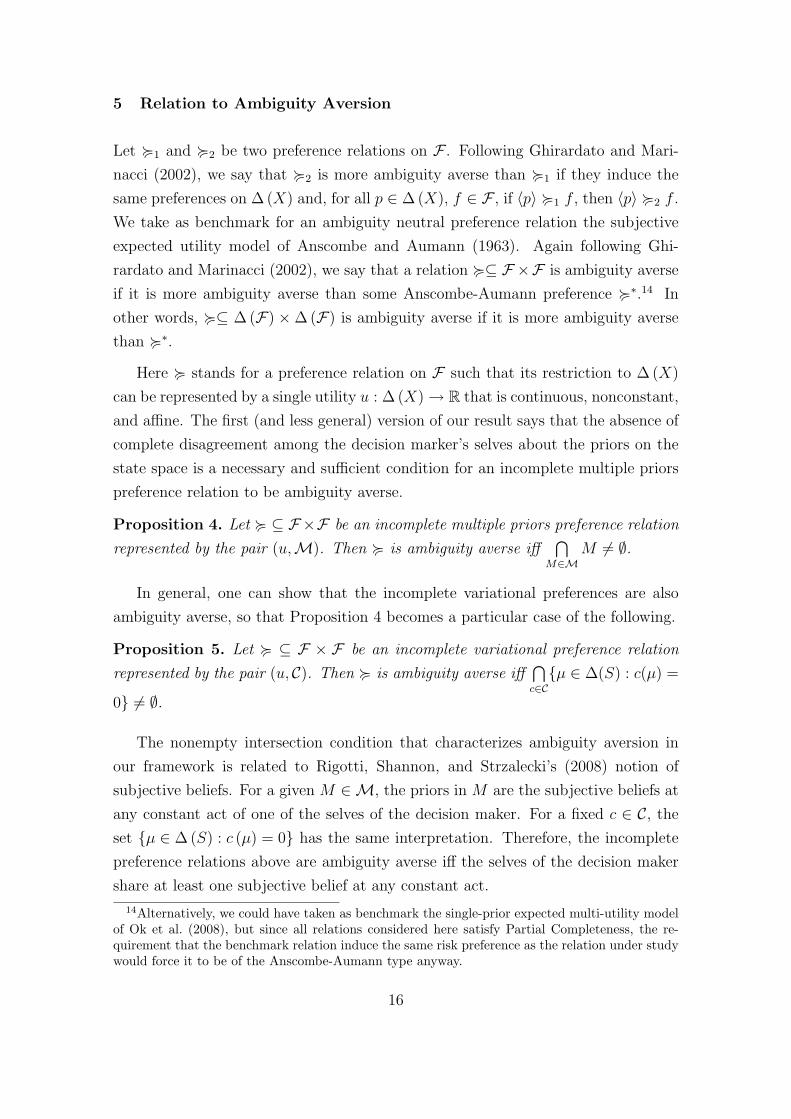
5 Relation to Ambiguity Aversion
Let <1 and <2 be two preference relations on F . Following Ghirardato and Mari-
nacci (2002), we say that <2 is more ambiguity averse than <1 if they induce the
same preferences on ∆ (X) and, for all p ∈ ∆ (X), f ∈ F , if 〈p〉 <1 f , then 〈p〉 <2 f .
We take as benchmark for an ambiguity neutral preference relation the subjective
expected utility model of Anscombe and Aumann (1963). Again following Ghi-
rardato and Marinacci (2002), we say that a relation <⊆ F ×F is ambiguity averse
if it is more ambiguity averse than some Anscombe-Aumann preference <∗.14 In
other words, <⊆ ∆ (F) ×∆ (F) is ambiguity averse if it is more ambiguity averse
than <∗.
Here < stands for a preference relation on F such that its restriction to ∆ (X)
can be represented by a single utility u : ∆ (X)→ R that is continuous, nonconstant,
and affine. The first (and less general) version of our result says that the absence of
complete disagreement among the decision marker’s selves about the priors on the
state space is a necessary and sufficient condition for an incomplete multiple priors
preference relation to be ambiguity averse.
Proposition 4. Let < ⊆ F×F be an incomplete multiple priors preference relation
represented by the pair (u,M). Then < is ambiguity averse iff⋂
M∈MM 6= ∅.
In general, one can show that the incomplete variational preferences are also
ambiguity averse, so that Proposition 4 becomes a particular case of the following.
Proposition 5. Let < ⊆ F × F be an incomplete variational preference relation
represented by the pair (u, C). Then < is ambiguity averse iff⋂c∈C{µ ∈ ∆(S) : c(µ) =
0} 6= ∅.
The nonempty intersection condition that characterizes ambiguity aversion in
our framework is related to Rigotti, Shannon, and Strzalecki’s (2008) notion of
subjective beliefs. For a given M ∈M, the priors in M are the subjective beliefs at
any constant act of one of the selves of the decision maker. For a fixed c ∈ C, the
set {µ ∈ ∆ (S) : c (µ) = 0} has the same interpretation. Therefore, the incomplete
preference relations above are ambiguity averse iff the selves of the decision maker
share at least one subjective belief at any constant act.
14Alternatively, we could have taken as benchmark the single-prior expected multi-utility modelof Ok et al. (2008), but since all relations considered here satisfy Partial Completeness, the re-quirement that the benchmark relation induce the same risk preference as the relation under studywould force it to be of the Anscombe-Aumann type anyway.
16

6 Towards a General Case
In this section we adapt the analysis of Cerreia-Vioglio et al. (2008) to the case of
incomplete preferences. We depart from the setup in the previous sections in the
sense that we do not work in an environment with lotteries of acts. The reason
is inherently technical. The analysis in Cerreia-Vioglio et al. (2008) is based on a
duality theory for monotone quasiconcave functions. The basic advantage of working
in an environment with lotteries of acts was the possibility of using the expected
multi-utility theory to derive a multi-utility representation with some particular
cardinal properties. Since quasiconcavity is an ordinal property, having an extra
layer of objective randomization in the present section would be of little use.
Formally, we consider a binary relation D on the domain of AA acts F , that
is, D⊆ F × F . Define the binary relation D•⊆ ∆ (X) × ∆ (X) by p D• q iff
〈p〉 D 〈q〉.The mixing operator + is defined so that, for all f, g ∈ F , λ ∈ [0, 1],
(λf + (1− λ) g) (s) (B) = λf (s) (B)+(1− λ) g (s) (B) for all s ∈ S, and B ∈ B (X).
Consider the following set of axioms on D .
Axiom B1 (Preference Relation). The binary relation D is a preorder.
Axiom B2 (Upper Semicontinuity). For all f ∈ F , the set {g ∈ F : g D f} is
closed.
Axiom B3 (Convexity). For all f ∈ F , the set {g ∈ F : g D f} is convex.
Axiom B4 (Monotonicity). For all f ∈ F : if 〈f (s)〉 D 〈g (s)〉 for all s ∈ S,
then f D g.
Axiom B5 (Partial Completeness). The binary relation D• is complete.
Axiom B6 (Weak Continuity). If (pn) , (qn) ∈ ∆ (X)∞ are such that pn D• qn
for all n, pn → p ∈ ∆ (X), and qn → q ∈ ∆ (X), then p D• q.
Axiom B7 (Risk Independence). For all p, q, r ∈ ∆ (X), λ ∈ (0, 1): if p D• q,
then λp+ (1− λ) r D• λq + (1− λ) r.
Axioms B5-B7 allow us to find an expected utility representation for the re-
lation D•. Axiom B4 is the same standard monotonicity property that was used
in the previous sections. Convexity of preferences is necessary to guarantee that
17

we can represent D by a set of quasiconcave functions. In the complete case this
property is replaced by Uncertainty Aversion, but in the presence of Completeness,
Monotonicity and Continuity they are equivalent.
Finally, we ask that D satisfy only Upper Semicontinuity. As pointed out by
Evren and Ok (2007), it is fairly easy to represent an upper semicontinuous pref-
erence relation by a set of upper semicontinuous functions. However, finding a
continuous multi-utility representation is a much more demanding task. Indeed, we
do not know of conditions that make D representable by a set of continuous and
quasiconcave functions. In any event, the postulates above are enough to give us a
multiple selves version of the representation in Cerreia-Vioglio et al. (2008).
Theorem 3. The following are equivalent:
(a) < satisfies B1-B7.
(b) There exist u : ∆ (X) → R continuous and affine, and a collection G of upper
semicontinuous functions (u.s.c.) G : u (∆ (X))×∆ (S)→ R such that:
1. For all f, g ∈ F ,
f D g
iff
infµ∈∆(S)
G
(∫u (f) dµ, µ
)≥ inf
µ∈∆(S)G
(∫u (g) dµ, µ
)for all G ∈ G.
2. For all µ ∈ ∆ (S), G ∈ G, G (·, µ) is increasing, and there exists H ∈ Gsuch that infµ∈∆(X) H (·, µ) is strictly increasing.
7 Discussion
7.1 Alternative axiomatization of variational preferences
The alternative axiomatization of the variational preferences of Maccheroni et al.
(2006) we propose is linked to the recent generalization of Cerreia-Vioglio et al.
(2008). Our goal in this alternative axiomatization is to show that one can dis-
pense with the weak c-independence axiom of Maccheroni et al. (2006), as we do in
our multiple selves version. All one needs is to replace it by independence on the
subdomain of constant acts plus a stronger monotonicity axiom.
18

The setup is the same as in sections 2 and 3, except that the binary relation
3 is defined on the domain of Anscombe-Aumann acts F . The restriction of 3 to
the subdomain of constant acts is denoted by 3•. A utility index U : F → R that
represents 3 can be constructed provided the following axioms are satisfied.
Axiom VP1 (Nondegenerate Weak Order). The binary relation 3 is a com-
plete preorder, and �6= ∅.
Axiom VP2 (Monotonicity). For all f ∈ F : if f (s) 3•g (s) for all s ∈ S, then
f 3 g.
Axiom VP3 (Risk Independence). For all p, q, r ∈ ∆ (X), λ ∈ (0, 1): if p 3• q,
then λp+ (1− λ) r 3• λq + (1− λ) r.
Axiom VP4 (Continuity). If (fn) , (gn) ∈ F∞ are such that fn 3 qn for all n,
fn → f ∈ F , and gn → g ∈ F , then f 3 g.
It is not difficult to check that axioms VP1-VP4 imply the existence of a non-
constant and affine function u ∈ C (∆ (X)) representing 3•, the existence of a
certainty equivalent pf for every act f , and that the function U : F → R defined
by U (f) = u (pf ) represents 3. Assume w.l.o.g. that u (∆ (X)) = [−1, 1].
Identify each f ∈ F with the vector of utils u (f) ∈ [−1, 1]S, and define the
preorder v on [−1, 1]S by u (f) = ξf v ξg = u (g) iff f % g. Because IU , as defined
by IU (ξf ) = U (f), represents v, this establishes the following lemma.
Lemma 1. There exists a nonconstant, continuous and monotonic function IU :
[−1, 1]S → R that represents v. Moreover, IU (a1S) = a for all a ∈ [−1, 1].
Two additional axioms are needed. One is the standard Uncertainty Aversion
axiom, and the other is a strengthening of the “uniform continuity” axiom of Cerreia-
Vioglio et al. (2008).15 We refer to our last axiom as “12-c-mixture monotonicity*”
because of its similarity with axiom A5’.
Axiom VP5 (Uncertainty Aversion). For all f, g ∈ F , λ ∈ (0, 1): if f ∼ g,
then λf + (1− λ) g 3 f .
15Cerreia-Vioglio et al. (2008) make use of an object (viz. the certainty equivalent of an act)that is not a primitive of the model to write that axiom. We avoid this issue here by adding oneadditional quantifier to our axiom VP6.
19
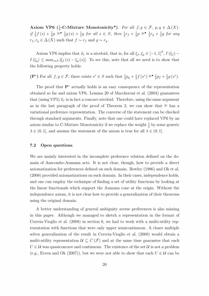
Axiom VP6 (12-C-Mixture Monotonicity*). For all f, g ∈ F , p, q ∈ ∆ (X):
if 12f (s) + 1
2p 3• 1
2g (s) + 1
2q for all s ∈ S, then 1
2rf + 1
2p 3• 1
2rg + 1
2q for any
rf , rg ∈ ∆ (X) such that f ∼ rf and g ∼ rg.
Axiom VP6 implies that IU is a niveloid, that is, for all ξf , ξg ∈ [−1, 1]S, I (ξf )−I (ξg) ≤ maxs∈S [ξf (s)− ξg (s)]. To see this, note that all we need is to show that
the following property holds:
(P∗) For all f, g ∈ F , there exists s∗ ∈ S such that 12pg + 1
2f (s∗) 3• 1
2pf + 1
2g (s∗).
The proof that P∗ actually holds is an easy consequence of the representation
obtained so far and axiom VP6. Lemma 20 of Maccheroni et al. (2004) guarantees
that (using VP5) IU is in fact a concave niveloid. Therefore, using the same argument
as in the last paragraph of the proof of Theorem 2, we can show that 3 has a
variational preference representation. The converse of the statement can be checked
through standard arguments. Finally, note that one could have replaced VP6 by an
axiom similar to C-Mixture Monotonicity if we replace the weight 12
by some generic
λ ∈ (0, 1], and assume the statement of the axiom is true for all λ ∈ (0, 1].
7.2 Open questions
We are mainly interested in the incomplete preference relation defined on the do-
main of Anscombe-Aumann acts. It is not clear, though, how to provide a direct
axiomatization for preferences defined on such domain. Bewley (1986) and Ok et al.
(2008) provided axiomatizations on such domain. In their cases, independence holds,
and one can employ the technique of finding a set of utility functions by looking at
the linear functionals which support the Aumann cone at the origin. Without the
independence axiom, it is not clear how to provide a generalization of their theorems
using the original domain.
A better understanding of general ambiguity averse preferences is also missing
in this paper. Although we managed to sketch a representation in the format of
Cerreia-Vioglio et al. (2008) in section 6, we had to work with a multi-utility rep-
resentation with functions that were only upper semicontinuous. A closer multiple
selves generalization of the result in Cerreia-Vioglio et al. (2008) would obtain a
multi-utility representation U ⊆ C (F) and at the same time guarantee that each
U ∈ U was quasiconcave and continuous. The existence of the set U is not a problem
(e.g., Evren and Ok (2007)), but we were not able to show that each U ∈ U can be
20

made quasiconcave and continuous at the same time.16,17
Finally, we conjecture that, provided we work with simple acts, our represen-
tations above (including section 6) would go through if we assume a general state
space S (not necessarily finite), and that the set of consequences is a convex and
compact metric space. We did not pursue such a path here because it would not
add much to our understanding of incomplete and ambiguity averse preferences.
A Appendix: Proofs
A.1 Proof of Theorem 1
The proof of the direction (b)⇒(a) is standard, and thus omitted. We now prove
(a)⇒(b).
Claim A.1.1. There exists a closed and convex set U ⊆ C (F) such that, for all
P,Q ∈ ∆ (F), P < Q iff∫F UdP ≥
∫F UdQ for all U ∈ U .
Proof of Claim A.1.1. Because F is a compact metric space, ∆ (F) is endowed with
the topology of weak convergence, and < satisfies A1-A3, the Expected Multi-Utility
Theorem of Dubra et al. (2004) applies.
Claim A.1.2. There exists an affine, continuous and nonconstant function u :
∆ (X)→ R such that, for all p, q ∈ ∆ (X), p <• q iff u (p) ≥ u (q).
Proof of Claim A.1.2. The binary relation <• is a preorder on ∆ (X). One can
verify A3 implies that <• is closed-continuous. Moreover, it is complete by A4.
Now use A2, A3, and A6 to obtain that, for all p, q, r ∈ ∆ (X), λ ∈ (0, 1), p <• q
iff 〈p〉 < 〈q〉 iff λ 〈p〉 ⊕ (1− λ) 〈r〉 ∼ λ 〈p〉 + (1− λ) 〈r〉 < λ 〈q〉 + (1− λ) 〈r〉 ∼λ 〈p〉 ⊕ (1− λ) 〈r〉 iff λp + (1− λ) r <• λq + (1− λ) r. Therefore, <• satisfies all
the assumptions of the Expected Utility Theorem, and it can be represented by an
affine and nonconstant function u ∈ C(∆ (X)). Moreover, using A5 and A8 one can
show u is nonconstant.18
16In particular, if the set U were compact and the function e : F → C (U) as defined bye (f) (u) = u (f) were K-quasiconcave in the sense of Benoist, Borwein, and Popovici (2002), onecould have applied their theorem 3.1. We were not successful in establishing those two properties.
17A general problem is that convex incomplete preferences may admit multi-utility representa-tions with some functions that fail to be quasiconcave.
18For any compact subset z of a normed vector space, C (z) stands for the set of continuousfunctions on z, and is endowed with the sup norm.
21

The set U may contain constant functions. They are not essential to the rep-
resentation and can be discarded at this point. Therefore, assume w.l.o.g. that Ucontains only nonconstant functions. By axiom A8, U 6= ∅.
We can employ standard arguments to prove the existence of x, x ∈ X such
that 〈δx〉 �• 〈δx〉, and 〈δx〉 <• 〈p〉 <• 〈δx〉 for all p ∈ ∆ (X). Moreover, because
of C-Reduction, Continuity, Partial Completeness and Independence over lotteries,
it can also be shown that, for all p ∈ ∆ (X), there exists λp ∈ [0, 1] such that
〈p〉 ∼ λp 〈δx〉 ⊕ (1− λp) 〈δx〉. The implication 〈p〉 � 〈q〉 ⇒ λp > λq is also true.
Fix any U ∈ U , and use Monotonicity to show that U (〈δx〉) > U (〈δx〉). As a
consequence, whenever 〈p〉 � 〈q〉, it is false that U (〈p〉) = U (〈q〉). If this equality
were true, then using axiom A6 and Independence on the subdomain of constant
acts we obtain
U (〈p〉) = λp (U (〈δx〉)− U (〈δx〉)) + U (〈δx〉)
= λq (U (〈δx〉)− U (〈δx〉)) + U (〈δx〉) = U (〈q〉) ,
implying (λp − λq) (U (〈δx〉)− U (〈δx〉)) = 0. Because of U (〈δx〉) > U (〈δx〉), we
have λp = λq, a contradiction. Conclusion: for any fixed U ∈ U , U |∆(X) is affine and
represents <•.
Claim A.1.3. Each U ∈ U can be normalized so that U |∆(X) = u.
Proof of Claim A.1.3. Fix any U ∈ U . Because <• is complete, for all p, q ∈ ∆ (X),
p <• q iff U (〈p〉) ≥ U (〈q〉). Therefore, U |∆(X) and u are both affine representations
of <•. By cardinal uniqueness, we know there exists (αU , βU) ∈ R++ ×R such that
U |∆(X) = αUu+ βU .
Because ∆ (X) is weak* compact and u is continuous, there exist p, p ∈ ∆ (X)
such that u (p) ≥ u (p) ≥ u(p)
for all p ∈ ∆ (X). By A5 and A8 it must be that p 6=p. W.l.o.g. normalize u so that u (p) = 1 and u
(p)
= −1. Then u (∆ (X)) = [−1, 1]
(use Second Stage Independence for constant acts). Given p ∈ ∆ (X), it follows from
our normalization of U in the previous step that U (〈p〉) = u (p). Therefore, for all
f ∈ F , let ξf := u ◦ f ∈ [−1, 1]S. Let the functional IU : [−1, 1]S → R be defined by
IU (ξf ) = U (f), for all ξf ∈ [−1, 1]S (A5 guarantees that IU is well-defined).
Claim A.1.4. IU is positively homogeneous.
Proof of Claim A.1.4. Take any U ∈ U . Let p0 ∈ ∆ (X) be such that u (p0) = 0.
Let ξf ∈ [−1, 1]S, λ ∈ (0, 1). Axiom A6 implies λf⊕(1− λ) 〈p0〉 ∼ λf+(1− λ) 〈p0〉,
22

and hence IU (λξf ) = U (λf + (1− λ) 〈p0〉) = λU (f) + (1− λ)U (〈p0〉) = λIU (ξf ).
If λ > 1 and λξf ∈ [−1, 1]S, then IU (ξf ) = IU(
1λ
(λξf ))
iff λIU (ξf ) = IU (λξf )
(because 1λ< 1).
Using an argument similar to Gilboa and Schmeidler (1989), we extend IU to RS
(call this extension I∗U): for all ξ ∈ RS, let I∗U (ξ) = 1λI∗U (λξ), for all λ > 0 such that
λξ ∈ [−1, 1]S. Standard arguments can be employed to show the extension does not
depend on which λ is used to shrink ξ towards the origin.
Claim A.1.5. I∗U is increasing, positively homogenous, superadditive, C-additive,
and normalized.
Proof of Claim A.1.5. Let ξ, ξ′ ∈ RS, and λ > 0 be such that λξ, λξ′ ∈ [−1, 1]S
and ξ ≥ ξ′. Then λξ ≥ λξ′, and by A5 we obtain that IU (λξ) = U (fλξ) ≥U (fλξ′) = IU (λξ′), where fλξ and fλξ′ are the acts associated with λξ and λξ′, re-
spectively. Hence I∗U (ξ) ≥ I∗U (ξ′), and I∗U is increasing. It is not difficult to verify I∗Uis positively homogeneous. For any ξ, ξ′ ∈ RS, I∗U
(12ξ + 1
2ξ′)
= 1λIU(λ(
12ξ + 1
2ξ′))
,
with λ > 0 being such that λ(
12ξ + 1
2ξ′), λ1
2ξ, λ1
2ξ′ ∈ [−1, 1]S. By A7 we obtain
IU(
12λξ + 1
2λξ′)≥ 1
2IU (λξ)+ 1
2IU (λξ′), and hence I∗U
(12ξ + 1
2ξ′)≥ 1
2I∗U (ξ)+ 1
2I∗U (ξ′).
Using positive homogeneity of I∗U we conclude that I∗U (ξ + ξ′) ≥ I∗U (ξ) + I∗U (ξ′),
and I∗U is superadditive. Now take ξ ∈ RS, a ∈ R, and let λ > 0 be such that
λ(
12ξ + 1
2a), λ1
2ξ, λ1
2a ∈ [−1, 1]S (with abuse of notation, we write a instead of
a1S). Using A6 we know that IU(
12λξ + 1
2λa)
= U(
12fλξ + 1
2〈pλa〉
)= 1
2U (fλξ) +
12U (〈pλa〉) = 1
2IU (λξ) + 1
2IU (λa), where u ◦ fλξ = λξ and u (pλa) = λa, with
fλξ, 〈pλa〉 ∈ F . Therefore, using positive homogeneity we obtain I∗U (ξ + a) =
I∗U (ξ) + I∗U (a), and I∗U is C-additive. It is clear that I∗U is normalized, that is,
I∗U (1) = 1.
Because, given any U ∈ U , I∗U satisfies all the properties proved in the previous
step, we can write I∗U (ξ) = minµ∈MU
∫ξdµ for all ξ ∈ RS, where MU is a closed
and convex subset of the |S| − 1-dimensional simplex (see Gilboa and Schmeidler
(1989)). Therefore, for all f ∈ F , U (f) = I∗U (u ◦ f) = minµ∈MU
∫u (f) dµ. Now
define M := {MU : U ∈ U}, and note that the pair (u,M) induces the desired
representation of < on ∆ (F).
A.2 Proof of Proposition 1
The proof of the “if” part is trivial and thus omitted. Let U ,V ⊆ C (F) be two
representations of < induced, respectively, by the pairs (u,M) and (v,N ). Because
23

both u and v represent <•, from the cardinal uniqueness of such a representation
it follows that u is a positive affine transformation of v. Also note that, from the
uniqueness of the expected multi-utility representation of Dubra et al. (2004), it
follows that cl‖·‖∞ (cone (U) + {θ1F : θ ∈ R}) = cl‖·‖∞ (cone (V) + {θ1F : θ ∈ R}).19
Now we prove two claims, which remain true if we replace U by V in their statements.
Claim A.2.1. For any nonconstant U ∈ cone (U) + {θ1F : θ ∈ R}, it is possible
to find (Ui)ni=1 ∈ Un, ρ ∈ ∆({1, ..., n}), and (α, β) ∈ R++ × R such that, U(f) =
minµ∈Σni=1ρiMUi
∫(αu(f) + β)dµ, for all f ∈ F , where, for all i ∈ {1, ..., n}, Ui (f) =
minµ∈MUi
∫u (f) dµ, for all f ∈ F .
Proof of Claim A.2.1. By definition, there exist (Ui)ni=1 ∈ Un, (γi)
ni=1 ∈ Rn
+\ {0},and β ∈ R such that U =
∑ni=1 γiUi + β, and then U = α
∑ni=1 ρiUi + β, where
α =∑n
i=1 γi and ρi = γi
αfor all i ∈ {1, ..., n}. Because every Ui can be written
as Ui (f) = −σMUi(−u (f)), where σMUi
stands for the support function of MUi, it
follows that U (f) = αminΣni=1ρiMUi
∫u (f) dµ+β (see, e.g., section 5.19 of Aliprantis
and Border (1999)).
Claim A.2.2. For any nonconstant U ∈ cl‖·‖∞ (cone (U) + {θ1F : θ ∈ R}), there
exist (α, β) ∈ R++ × R, and M ∈ cldH(co (M)) such that, for all f ∈ F , U (f) =
minµ∈M∫
(αu (f) + β) dµ.
Proof of Claim A.2.2. We can take (Un) ∈ (cone (U) + {θ1F : θ ∈ R})∞, where each
Un is nonconstant w.l.o.g., and such that Un → U . For all n ∈ N, f ∈ F , Un (f) =
αn (−σMn (−u (f))) + βn. Let p, q ∈ ∆ (X) be such that u (p) > u (q). Because (Un)
also converges pointwise, limn [αnu (p) + βn] = U (〈p〉) and limn [αnu (q) + βn] =
U (〈q〉), which implies limn αn [u (p)− u (q)] = U (〈p〉) − U (〈q〉). Hence αn → α ≥0, and indeed α > 0 because U is nonconstant. Therefore βn → β, for some
β ∈ R. Now use the fact M is compact to obtain a convergent subsequence (Mnk),
and clearly Mnk→dH
M ∈ cldH(co (M)). Each σMn is a real-valued function on
u (∆ (X))S, which is compact. Then(σMnk
)converges uniformly to σM .20
From claims A.2.1 and A.2.2, it follows that cl (cone (U) + {θ1F : θ ∈ R}) =
{U ∈ C (F) : U (f) = minµ∈M∫
(αu (f) + β) dµ, α ≥ 0, β ∈ R, M ∈ cldH(co (M))},
where a similar equality holds if U is replaced by V . Now use the uniqueness re-
sults of Dubra et al. (2004) and Gilboa and Schmeidler (1989) to conclude that
cldH(co (M)) = cldH
(co (N )).
19For any subset z of a vector space, cone (z) is the smallest convex cone which contains z.20This last part follows from Hirirart-Urruty and Lemarechal (2001, Corollary 3.3.8, p.156)
24

A.3 Proof of Proposition 2
Claim A.3.1. Fix any f, g ∈ F . There exists s∗ ∈ S such that 12〈g (s)〉 +
12〈f (s∗)〉 < 1
2〈f (s)〉+ 1
2〈g (s∗)〉 for all s ∈ S.
Proof of Claim A.3.1. Assume by way of contradiction this is not the case. Then,
using Reduction of Lotteries and Partial Completeness, for any si ∈ S there exists
sj such that1
2〈g (sj)〉+
1
2〈f (si)〉 ≺
1
2〈f (sj)〉+
1
2〈g (si)〉 .
Enumerate S = {s1, ..., sn} and let sn1 := s1. If k ≥ 1, let nk+1 be such that
1
2
⟨g(snk+1
)⟩+
1
2〈f (snk
)〉 ≺ 1
2
⟨f(snk+1
)⟩+
1
2〈g (snk
)〉 .
Let l > 1 be the smallest integer to satisfy snl+1∈ {sn1 , ..., snl
}. Then snl+1= snk
for some k ∈ {1, ..., l − 1}, and by the repeated application of A2, A4, and A6’, one
obtains
l+1∑o=k+1
1
Nl,k
〈g (sno)〉+l∑
o=k
1
Nl,k
〈f (sno)〉 ≺l+1∑
o=k+1
1
Nl,k
〈f (sno)〉+l∑
o=k
1
Nl,k
〈g (sno)〉 ,
where Nl,k := 2 (l + 1− k) and the summation symbol∑
operates w.r.t. the mix-
ture operation “+”. This contradicts reflexivity as the lotteries of acts on both sides
are the same.
Now use A5’ to obtain 12g + 1
2〈f (s∗)〉 < 1
2f + 1
2〈g (s∗)〉.
A.4 Proof of Theorem 2
The proof of the direction (b)⇒(a) is standard, and thus omitted. We now prove
(a)⇒(b).
Use claims A.1.1, A.1.2 and A.1.3 to obtain a set U ⊆ C (F) such that, for all
P,Q ∈ ∆ (F), P < Q iff∫F UdP ≥
∫F UdQ for all U ∈ U , and each U satisfies
U |∆(X) = u, for some affine u ∈ C (∆ (X)) with u (∆ (X)) = [−1, 1]. For all U , let
the functional IU : [−1, 1]S → R be defined as IU (ξf ) = U (f).
Take any U ∈ U , ξf , ξg ∈ [−1, 1]S. Using A1, A2, A4, A5’ and A6’, Proposition
2 implies the existence of s∗ ∈ S such that 12IU (ξg) + 1
2ξf (s∗) ≥ 1
2IU (ξf ) + 1
2ξg (s∗),
which is the case iff IU (ξf )−IU (ξg) ≤ maxs∈S [ξf (s)− ξg (s)]. Moreover, A7 implies
25

that for all f, g ∈ F , λ ∈ (0, 1), IU(λξf + (1− λ) ξg) ≥ λIU (ξf ) + (1− λ) IU (ξg).
Therefore IU is a concave niveloid. Moreover, for any a ∈ [−1, 1], we have, for some
p ∈ ∆ (X), IU (a) = U (〈p〉) = u (〈p〉) = a. Hence IU is also normalized.
By putting together Lemma 24, Corollary 28 and Remark 3 of Maccheroni et al.
(2004), we obtain that, for all U ∈ U , there exists a l.s.c., grounded and convex
function cU : ∆ → R+ such that, for all ξf , IU (ξf ) = minµ∈∆
[∫ξfdµ+ cU (µ)
].
Define C := {cU : U ∈ U}, and note that the pair (u, C) yields the desired repre-
sentation of < on ∆ (F). The proof that, for each cU , there exists a minimal c∗Udefined as c∗U (µ) := −minf∈F
{∫u (f) dµ− U (f)
}is a consequence of Lemma 27
of Maccheroni et al. (2004).
A.5 Proof of Proposition 3
The proof of the “if” part is trivial and thus omitted. Let U ,V ⊆ C (F) be two
representations of < induced, respectively, by the pairs (u, C) and (v, E) with mininal
cost functions. Therefore, U |∆(X) = u and V |∆(X) = v for all (U, V ) ∈ U × V . (In
this case we say that U and V are normalized.)
Claim A.5.1. For any nonconstant V ∈ cone (V) + {θ1F : θ ∈ R}, there exist(α, β
)∈ R++ × R and a nonconstant V ∈ co (V) such that V = αV + β.
Proof of Claim A.5.1. For some n ∈ N, there exist λ ∈ Rn+\ {0}, V1, ..., Vn ∈ V , and
θ ∈ R such that V =∑n
i=1 λiVi + θ. Now define α :=∑n
i=1 λi > 0 and β := θ, and
note that V = αV + β, where V := 1αV ∈ co (V) is nonconstant.
Claim A.5.2. For any nonconstant V ∈ cl‖·‖∞ (cone (V) + {θ1F : θ ∈ R}), there
exist(α, β
)∈ R++×R and a nonconstant V ∈ cl‖·‖∞ (co (V)) such that V = αV +β.
Proof of Claim A.5.2. Let (Vn) ∈ (cone (V) + {θ1F : θ ∈ R})∞ be such that Vn →V . Using Claim 1, each Vn = αnV n + βn, for some
(αn, βn
)∈ R++ × R and
V n ∈ co (V). Let p, q ∈ ∆ (X) be such v (p) > v (q), and note that Vn → V implies
that Vn (〈p〉)−Vn (〈q〉)→ V (〈p〉)−V (〈q〉), which is equivalent to αn [v (p)− v (q)]→V (〈p〉) − V (〈q〉). Therefore, there exists α ≥ 0 such that αn → α. Because V is
nonconstant, we have α > 0. Using the fact that αnv (p)+βn → V (〈p〉), we conclude
that βn → β, for some β ∈ R. Conclusion: V = limn
(αnV n + βn
)= αV + β, and
V is nonconstant.
Claim A.5.3. If U ,V ⊆ C (F) are normalized, then they represent < iff there exists
(α, β) ∈ R++ × R such that cl‖·‖∞ (co (U)) = α[cl‖·‖∞ (co ( V))
]+ β.
26
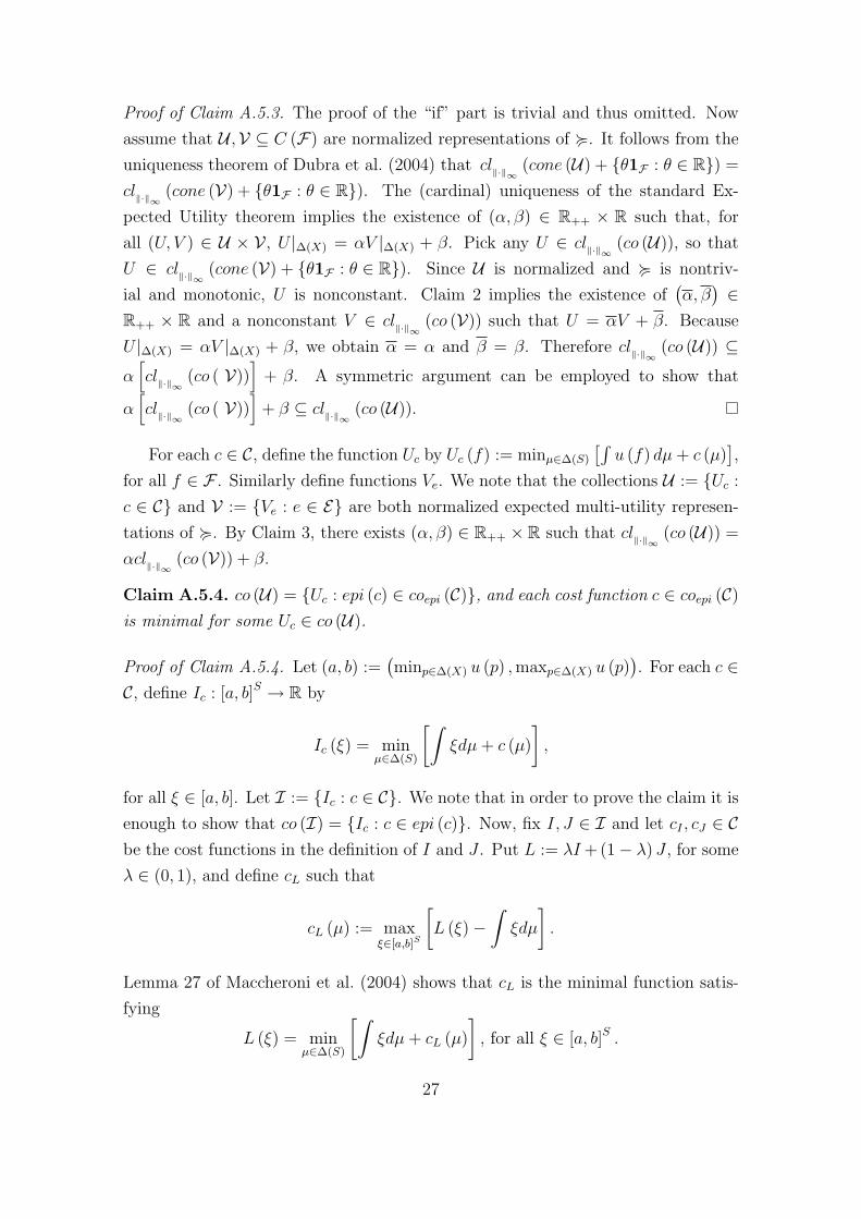
Proof of Claim A.5.3. The proof of the “if” part is trivial and thus omitted. Now
assume that U ,V ⊆ C (F) are normalized representations of <. It follows from the
uniqueness theorem of Dubra et al. (2004) that cl‖·‖∞ (cone (U) + {θ1F : θ ∈ R}) =
cl‖·‖∞ (cone (V) + {θ1F : θ ∈ R}). The (cardinal) uniqueness of the standard Ex-
pected Utility theorem implies the existence of (α, β) ∈ R++ × R such that, for
all (U, V ) ∈ U × V , U |∆(X) = αV |∆(X) + β. Pick any U ∈ cl‖·‖∞ (co (U)), so that
U ∈ cl‖·‖∞ (cone (V) + {θ1F : θ ∈ R}). Since U is normalized and < is nontriv-
ial and monotonic, U is nonconstant. Claim 2 implies the existence of(α, β
)∈
R++ × R and a nonconstant V ∈ cl‖·‖∞ (co (V)) such that U = αV + β. Because
U |∆(X) = αV |∆(X) + β, we obtain α = α and β = β. Therefore cl‖·‖∞ (co (U)) ⊆α[cl‖·‖∞ (co ( V))
]+ β. A symmetric argument can be employed to show that
α[cl‖·‖∞ (co ( V))
]+ β ⊆ cl‖·‖∞ (co (U)).
For each c ∈ C, define the function Uc by Uc (f) := minµ∈∆(S)
[∫u (f) dµ+ c (µ)
],
for all f ∈ F . Similarly define functions Ve. We note that the collections U := {Uc :
c ∈ C} and V := {Ve : e ∈ E} are both normalized expected multi-utility represen-
tations of <. By Claim 3, there exists (α, β) ∈ R++ × R such that cl‖·‖∞ (co (U)) =
αcl‖·‖∞ (co (V)) + β.
Claim A.5.4. co (U) = {Uc : epi (c) ∈ coepi (C)}, and each cost function c ∈ coepi (C)is minimal for some Uc ∈ co (U).
Proof of Claim A.5.4. Let (a, b) :=(minp∈∆(X) u (p) ,maxp∈∆(X) u (p)
). For each c ∈
C, define Ic : [a, b]S → R by
Ic (ξ) = minµ∈∆(S)
[∫ξdµ+ c (µ)
],
for all ξ ∈ [a, b]. Let I := {Ic : c ∈ C}. We note that in order to prove the claim it is
enough to show that co (I) = {Ic : c ∈ epi (c)}. Now, fix I, J ∈ I and let cI , cJ ∈ Cbe the cost functions in the definition of I and J . Put L := λI + (1− λ) J , for some
λ ∈ (0, 1), and define cL such that
cL (µ) := maxξ∈[a,b]S
[L (ξ)−
∫ξdµ
].
Lemma 27 of Maccheroni et al. (2004) shows that cL is the minimal function satis-
fying
L (ξ) = minµ∈∆(S)
[∫ξdµ+ cL (µ)
], for all ξ ∈ [a, b]S .
27

Let cλ be the function that satisfies epi (cλ) = λepi (cI) + (1− λ) epi (cJ). We want
to prove that cL = cλ.
Following Maccheroni et al. (2004), for A = I, J, L, we extend A to [a, b]S + Rusing vertical invariance of A. Call this extension A. Now, we further extend A to
RS by
A (ξ) = max(κ ∈ R : ∃ξ ∈ [a, b]S + R with ξ − κ ≥ ξ and A
(ξ)≥ 0).
Lemma 24 of Maccheroni et al. (2004) shows that A is the minimum niveloid that
extends A to RS. For each ξ ∈ RS, define ξ such that
ξs := min
{ξs,min
s∈S{ξs}+ (b− a)
}.
Note that ξ ≥ ξ and that ξ ∈ [a, b]S + R. Moreover, ξ − A(ξ) ≥ ξ − A(ξ) and
A(ξ−A(ξ)) = A(ξ)−A(ξ) = 0. For any ε > 0 and ζ ∈ [a, b]S+R, if ξ−A(ξ)−ε ≥ ζ,
then ξ − A(ξ) ≥ ζ. Therefore A (ξ) = A(ξ), for A = I, J, L.
Now we show that L = λI + (1− λ) J . First note that for all (ξ, κ) ∈ [a, b]S×R,
L (ξ + κ) = L (ξ) + κ
= λ (I (ξ) + κ) + (1− λ) (J (ξ) + κ)
= λI (ξ + κ) + (1− λ) J (ξ + κ) .
Using the fact A (ξ) = A(ξ) for all ξ ∈ [a, b]S, A = I, J, L, we obtain
L (ξ) = L(ξ)
= λI(ξ)
+ (1− λ) J(ξ)
= λI (ξ) + (1− λ) J (ξ) .
From Lemma 27 of Maccheroni et al. (2004), we know that cA, for A = I, J, L is
the unique l.s.c. and convex function such that
A (ξ) = minµ∈∆(S)
[∫ξdµ+ cA (µ)
], for all ξ ∈ RS.
28

It can be easily checked that
λI (ξ) + (1− λ) J (ξ) = minµ∈∆(S)
[∫ξdµ+ cλ (µ)
], for all ξ ∈ RS.
Conclusion: cL = cλ. A simple inductive argument completes the proof of the
claim.
Claim A.5.5. cl‖·‖∞ (co (U)) ={Uc : c ∈ cl‖·‖∞ (coepi (C))
}, and each cost function
c ∈ cl‖·‖∞ (coepi (C)) is minimal for some Uc ∈ cl‖·‖∞ (co (U)).
Proof of Claim A.5.5. By the previous claim, co (U) = {Uc : c ∈ coepi (C)} and all
c ∈ coepi (C) are minimal, so it is enough to show that for any sequence ( cn) ∈(coepi (C))∞, cn → c if and only if Ucn → Uc and c is the minimal cost function
associated to Uc. Suppose that Ucn → Uc, where c is the minimal cost function
associated to Uc. Fix ε > 0. There exists N ∈ N such that, for all f ∈ F ,
|Ucn (f)− Uc (f)| < ε for all n > N . Each e ∈ {c} ∪ {cn}∞n=1 satisfies:
e (µ) = maxf∈F
[Ue (f)−
∫u (f) dµ
].
Fix some µ ∈ ∆ (S), and let fc and {fn}∞n=1 be the maximizers associated to c (µ)
and {cn}∞n=1, respectively, in the expression above. We note that, for all n > N ,
Uc (fc)−Ucn (fc) < ε. This implies that, for all n > N , cn (µ) > c (µ)− ε. Similarly,
for all n > N , Ucn (fn) − Uc (fn) < ε. Again, this implies that, for all n > N ,
c (µ) > cn (µ) − ε. We conclude that, for all n > N , |c (µ)− cn (µ)| < ε. Since µ
is arbitrary, (cn) converges uniformly to c. We can perform a similar analysis using
the fact that for each c,
Uc (f) = minµ∈∆(S)
[∫u (f) dµ− c (µ)
]to show that uniform convergence of the functions (cn) implies uniform convergence
of the functions Ucn . By what we have proved before this will, in turn, imply that
c is minimal, which completes the proof of the claim.
To complete the proof of the proposition, we simply observe that for any U
with variational representation (u, c), for all (α, β) ∈ R++ × R, the variational
representation of αU + β is (αu+ β, αc).
29

A.6 Proof of Proposition 5
Assume that there exists some µ∗ ∈⋂c∈C
Mc, where Mc := {µ ∈ ∆ (S) : c (µ) = 0}. If
(p, f) ∈ ∆ (X)×F is such that u (p) ≥∫u (f) dµ∗, then u (p) ≥
∫u (f) dµ∗+c (µ∗) ≥
minµ∈∆(S)
{∫u (f) dµ+ c (µ)
}for all c ∈ C.
Now suppose that⋂c∈C
Mc = ∅, and assume w.l.o.g. that u (∆ (X)) = [−1, 1]. For
all ε > 0, define M εc := {µ ∈ ∆ (S) : c (µ) ≤ ε}.
Claim A.6.1. If⋂c∈C
Mc = ∅, then there exists ε > 0 such that⋂c∈C
M εc = ∅.
Proof of Claim A.6.1. Suppose that⋂c∈C
M εc 6= ∅ for all ε > 0. Then for all n ∈ N
there exists µn ∈ ∆ (S) such that c (µn) ≤ 1n
for all c ∈ C. Use compactness of ∆ (S)
to extract a subsequence (µnk) such that µnk
→ µ for some µ ∈ ∆ (S). For any fixed
c ∈ C we use the l.s.c. of c to obtain c (µ) ≤ lim inf c (µnk) ≤ lim inf 1
nk= 0, thus
contradicting⋂c∈C
Mc = ∅.
From the previous claim, we know there exists some ε > 0 such that⋂c∈C
M εc = ∅.
Fix any µ∗ and note that µ∗ /∈M εc for some c ∈ C. Because c is convex and l.s.c., the
nonempty set M εc is closed and convex. Using the Separating Hyperplane Theorem
we can find uf ∈ [−1, 1]S such that∫ufdµ
∗ <∫ufdµ for all µ ∈ M ε
c . We can also
assume w.l.o.g. that∣∣∫ ufdµ∣∣ < ε
3for all µ ∈ ∆ (S).
Now pick p ∈ ∆ (X) such that u (p) =∫ufdµ
∗ and note that, by construction,
u (p) <∫ufdµ + c (µ) for all µ ∈ M ε
c . Hence u (p) < minµ∈Mεc
{∫ufdµ+ c (µ)
},
where in the last inequality we used the fact M εc is compact. For all µ ∈ ∆ (X) \M ε
c
we have u (p) < ε3< 2ε
3<∫ufdµ+ c (µ). As a consequence, since ∆ (S) is compact,
we must have u (p) < minµ∈∆(S)
{∫ufdµ+ c (µ)
}. Let f ∈ F be such that u (f) =
uf , and <∗ be the Anscombe-Aumann preference relation induced by the pair (u, µ∗).
Therefore 〈p〉 ∼∗ f , but ¬ 〈p〉 < f . Because µ∗ was arbitrary, this implies < is not
ambiguity averse.
A.7 Proof of Theorem 3
Claim A.7.1. Let a, b ∈ R, b > a, and V : [a, b]S → R. The following are equivalent:
(i) V is increasing, u.s.c., and quasiconcave.
30

(ii) There exists an u.s.c. function G : [a, b] × ∆ (S) → R such that, for all ξ ∈[a, b]S,
V (ξ) = infµ∈∆(S)
G
(∫ξdµ, µ
),
and, for all µ ∈ ∆ (S), G (·, µ) is increasing.
Proof of Claim A.7.1. (i)⇒(ii). Define V : RS → R∪{−∞} by V (ξ) := sup{V (ζ) :
ζ ∈ [a, b]S and ζ ≤ ξ}. It can be checked that V is an increasing, u.s.c., and
quasiconcave extension of V . Now define the function V : R×∆ (S)→ R ∪ {−∞}as G (r, µ) := supξ∈RS{V (ξ) :
∫ξdµ ≤ r}. By construction, for any fixed ξ ∈ RS,
V (ξ) ≤ G(∫
ξdµ, µ)
for all µ ∈ ∆ (S); hence V (ξ) ≤ infµ∈∆(S) G(∫
ξdµ, µ). If
{ζ ∈ RS : V (ζ) ≥ V (ξ)} = ∅, then infµ∈∆(S) G(∫
ξdµ, µ)≤ V (ξ). Otherwise, there
exists ε > 0 such that Γε := {ζ ∈ RS : V (ζ) ≥ V (ξ) + ε} 6= ∅ for all ε ∈ (0, ε].
Because Γε is closed and convex, and ξ /∈ Γε, by the Separating Hyperplane Theorem
there exists q ∈ RS \ {0} such that∫ζdq >
∫ξdq for all ζ ∈ Γε. Since V is
increasing, q ∈ RS+ \ {0}. Therefore, it is w.l.o.g. to take ν ∈ ∆ (S) such that∫
ζdν >∫ξdν for all ζ ∈ Γε. This implies that G
(∫ξdν, ν
)≤ V (ξ) + ε and,
consequently, infµ∈∆(S) G(∫
ξdµ, µ)≤ V (ξ) + ε. Since ε ∈ (0, ε] was arbitrary, we
obtain infµ∈∆(S) G(∫
ξdµ, µ)≤ V (ξ). Conclusion: V (ξ) = infµ∈∆(S) G
(∫ξdµ, µ
)for all ξ ∈ RS.
Now let α ∈ R be such that A := {(r, µ) ∈ R × ∆ (S) : G (r, µ) ≥ α} 6= ∅.Let (rn, µn) ∈ A∞ satisfy (rn, µn) → (r, µ). For all n, pick ξn ∈ [a, b]S such that∫ξndµn ≤ rn and V (ξn) ≥ V (ζ). The existence of ξn follows from the way V and
G were constructed. Note that, we can assume w.l.o.g. that ξn → ξ, by passing to
a subsequence if necessary. Clearly,∫ξdµ ≤ r, so that G (r, µ) ≥ V (ξ). Because
V (ξn) ≥ α for all n, and V is u.s.c., we conclude that V (ξ) ≥ α, implying that
G (r, µ) ≥ α. Therefore G is u.s.c.. It is also increasing in the first argument, as it can
be easily checked. Put G := G|[a,b]×∆(S) and note that V (ξ) = infµ∈∆(S) G(∫
ξdµ, µ)
for all ξ ∈ [a, b]S.
(ii)⇒(i). Let ξ, ζ ∈ [a, b]S be such that ξ ≥ ζ. For all µ ∈ ∆ (S), V (ζ) ≤G(∫
ζdµ, µ)≤ G
(∫ξdµ, µ
), where the last inequality follows from the fact G (·, µ)
is increasing. Therefore V (ζ) ≤ infµ∈∆(S) G(∫
ξdµ, µ)
= V (ξ), and V must be
increasing. Now let λ ∈ (0, 1) and ξ and ζ be any two elements in [a, b]S. For all
31

µ ∈ ∆ (S),
G
(λ
∫ξdµ + (1− λ)
∫ζdµ, µ
)≥ min
{G
(∫ξdµ, µ
), G
(∫ζdµ, µ
)}≥ min
{inf
µ∈∆(S)G
(∫ξdµ, µ
), infµ∈∆(S)
G
(∫ζdµ, µ
)}.
Hence V (λξ+(1−λ)ζ) = infµ∈∆(S) G(λ∫ξdµ+(1−λ)
∫ζdµ, µ) ≥ min{V (ξ) , V (ζ)},
implying V is quasiconcave. Finally, let α ∈ R be such that B := {ζ ∈ [a, b]S :
V (ζ) ≥ α} 6= ∅, and take a sequence (ξn) ∈ B∞ such that ξn → ξ. By construction,
G(∫ξndµ, µ) ≥ V (ξn) ≥ α for all n ∈ N, for all µ ∈ ∆(S). Because G is u.s.c., we
must have G(∫
ξdµ, µ)≥ α, and hence V (ξ) ≥ α.
Claim A.7.2. Every upper semicontinuous and convex preorder can be represented
by a set of upper semicontinuous and quasiconcave utility functions.
Proof of Claim A.7.2. Adapt the arguments of Evren and Ok (2007) and Kochov
(2007). (The representation is induced by the set of indicator functions of the upper
contour sets of all elements on the domain of preferences.)
(a)⇒(b). Standard arguments can be employed to show the existence of a con-
tinuous and affine function u : ∆ (X)→ R such that, for all p, q ∈ ∆ (X), p D• q iff
u (p) ≥ u (q). Now every act f ∈ F can mapped into a vector of utils ξf := u (f) ∈u (∆ (X))S. We can also define a binary relation %⊆ u (∆ (X))S × u (∆ (X))S so
that, for all ξf , ξg ∈ u (∆ (X))S, ξf % ξg iff f D g. The monotonicity axiom B4
guarantees % is well-defined. It is easy to see that % is a monotonic preorder. Now
take any sequence (ξfn) in u (∆ (X))S such that ξfn % ξg for all n ∈ N, some g ∈ F, and ξfn → ξ. Because F is a compact metric space, we may assume, by passing
to a subsequence if necessary, that fn → f , for some f ∈ F . As a consequence,
using the continuity axiom B2, we conclude ξ = ξf % ξg. Therefore % is upper
semicontinuous. It is a standard exercise to show % is also convex. Now apply claim
A.7.2 to find a set V of u.s.c. and quasiconcave function such that, for all f, g ∈ F ,
f D g iff ξf % ξg iff V (ξf ) ≥ V (ξg) for all V ∈ V . Monotonicity of % implies each
V ∈ V must be increasing.
For all c ∈ u (∆ (X)), let Vc denote the function in V which takes the value 1
when evaluated at ξf with ξf % c1S, and 0 otherwise. Consider the enumeration
{d1, d2, ...} of the set D := u (∆ (X))∩Q, and define the function W :=∑∞
i=112iVdi
.
32

Because W is the uniform limit of a sequence of u.s.c. functions, it is itself a u.s.c.
function. Now we show W is quasiconcave. For all j ∈ N, define Wj :=∑j
i=112iVdi
and εj :=∑∞
i=j+112i > 0. Let α ∈ (0, 1], and f, g ∈ F be such that W (ξf ) ≥ α and
W (ξg) ≥ α. Note Wj (ξf ) ≥ α − εj and Wj (ξg) ≥ α − εj. For some j such that
α − εj > 0, put d∗j :={d ∈ {d1, ..., dj} :
∑ji=1
12iVdi
(d) ≥ α− εj}
. By construction,
d∗j is well-defined. Because Wj (ξf ) ≥ α− εj, we must have ξf % d∗j1S, for otherwise
¬ξf % d∗j1S implies Vd (f) = 0 for all d ≥ d∗j . As a consequence, in order to
attain Wj (ξf ) ≥ α− εj, we must have∑j
i=112iVdi
(d∗) ≥ α− εj for some d∗ < d∗j , a
contradiction with the definition of d∗j . A similar argument can be employed to show
ξg % d∗j1S. Because % is convex, for all λ ∈ (0, 1), we have λξf + (1− λ) ξf % d∗j1S,
which in turn implies W (λξf + (1− λ) ξf ) ≥ W(d∗j)≥ α − εj +
∑∞i=j+1
12iVdi
(d∗j).
If we let j →∞, we obtain W (λξf + (1− λ) ξf ) ≥ α. Therefore, W is quasiconcave.
Also note that, for all c, d ∈ u (∆ (X)), c ≥ d iff W (c) ≥ W (d). Moreover, we can
consider V ∪{W} instead of V , and infµ∈∆(X) H (·, µ) is strictly increasing for all
µ ∈ ∆ (S), where H : u (∆ (X)) × ∆ (S) → R is defined as in the proof of claim
A.7.1.
(b)⇒(a). First note that, for all p, q ∈ ∆ (X), p D• q iff u (p) ≥ u (q). Clearly
u(p) ≥ u(q) impliesG(u(p), µ) ≥ G(u(q), µ). As a consequence infµ∈∆(S) G(u(p)), µ ≥infµ∈∆(S) G(u(q), µ) and p D• q. Now assume u(p) > u(q), then infµ∈∆(S) H(u(p), µ) >
infµ∈∆(S) H(u(q), µ), and infµ∈∆(S) G(u(p), µ) ≥ infµ∈∆(S) G(u(q), µ) for all other
G ∈ G. This implies p B q. Therefore, u is an expected utility representation
of D•, and D• must satisfy B5-B7. Second, let (fn) ∈ F∞ be such that fn < g ∈ Ffor all n ∈ N. Fix any G ∈ G, and note that infµ∈∆(S) G
(∫u (fn) dµ, µ
)≥
infµ∈∆(S) G(∫
u (g) dµ, µ). As the pointwise infimum of a family of u.s.c. functions,
ξ 7→ infµ∈∆(S) G(∫
ξdµ, µ)
is itself a continuous function. Since u(fn) → u(f), we
obtain
infµ∈∆(S)
G
(∫u (f) dµ, µ
)= lim
ninf
µ∈∆(S)G
(∫u(fn)dµ, µ
)≥ inf
µ∈∆(S)G
(∫u (g) dµ, µ
)).
Therefore, < is u.s.c. Third, let f, g < h, λ ∈ (0, 1), and G ∈ G. Because G (·, µ)
is increasing and λu (f) + (1− λ)u (g) ≥ min {u (f) , u (g)}, one obtains, for all
33

µ ∈ ∆ (S),
G
(∫u(λf + (1− λ) g)dµ, µ
)≥ min{G
(∫u (f) dµ, µ
), G
(∫u (g) dµ, µ
)}
≥ min{ infµ∈∆(S)
G
(∫u (f) dµ, µ
), infµ∈∆(S)
G
(∫u (g) dµ, µ
)}
≥ infµ∈∆(S)
G
(∫u (h) dµ, µ
).
Hence infµ∈∆(S) G(∫
u (λf + (1− λ) g) dµ, µ)≥ infµ∈∆(S) G
(∫u (h) dµ, µ
). Since
G ∈ G was arbitrary, then λf + (1− λ) g < h, and < must be convex. Finally,
let f, g ∈ F be such that f (s) D• g (s) for all s ∈ S. Therefore∫u (f) dµ ≥∫
u (g) dµ for all µ ∈ ∆ (S) and, since G (·, µ) is an increasing function, we obtain
that infµ∈∆(S) G(∫
u (f) dµ, µ)≥ infµ∈∆(S) G
(∫u (g) dµ, µ
)for all G ∈ G.
References
Aliprantis, C. and K. Border (1999). Infinite Dimensional Analysis (2nd ed.).
Springer.
Anscombe, F. and R. Aumann (1963). A definition of subjective probability. The
Annals of Mathematical Statistics 34, 199–205.
Aumann, R. (1962). Utility theory without the completeness axiom. Economet-
rica 30, 445–462.
Benoist, J., J. Borwein, and N. Popovici (2002). A characterization of quasiconvex
vector-valued functions. Proceedings of the American Mathematical Society 131,
1109–1113.
Bewley, T. (1986). Knightian decision theory: Part i. Cowles Foundation Discussion
Papers .
Camerer, C. (1995). Individual decision making. In J. Kagel and A. Roth (Eds.), The
Handbook of Experimental Economics, pp. 587–703. Princeton University Press.
Cerreia-Vioglio, S., F. Maccheroni, M. Marinacci, and L. Montrucchio (2008). Un-
certainty averse preferences. manuscript.
34
Dolecki, S. and G. Greco (1991). Niveloides: fonctionnelles isotones commutant avec
l’addition de constantes finies. Comptes Rendus de l’Academie des Sciences. Serie
I. Mathematique 312, 113–118.
Dolecki, S. and G. Greco (1995). Niveloids. Topological Methods in Nonlinear
Analysis 5, 1–22.
Dubra, J., F. Maccheroni, and E. Ok (2004). Expected utility theory without the
completeness axiom. Journal of Economic Theory 115, 118–133.
Eliaz, K. and E. Ok (2006). Indifference or indecisiveness? choice theoretic founda-
tions of incomplete preferences. Games and Economic Behavior 56, 61–86.
Ellsberg, D. (1961). Risk, ambiguity, and the savage axioms. The Quarterly Journal
of Economics 75, 643–669.
Ellsberg, D. (2001). Risk, Ambiguity and Decisions. Gerland Publishing.
Epstein, L., M. Marinacci, and K. Seo (2007). Coarse contingencies and ambiguity.
Theoretical Economics 2, 355–394.
Evren, O. and E. Ok (2007). On the multi-utility representation of preference rela-
tions. manuscript.
Faro, J. (2008). General ambiguity index for bewley preferences. manuscript.
Ghirardato, P. and M. Marinacci (2002). Ambiguity made precise: A comparative
foundation. Journal of Economic Theory 102, 251–289.
Gilboa, I. and D. Schmeidler (1989). Maxmin expected utility with non-unique
prior. Journal of Mathematical Economics 18, 141–153.
Halevy, Y. (2007). Ellsberg revisited: an experimental study. Econometrica 75,
503–536.
Hirirart-Urruty, J.-B. and C. Lemarechal (2001). Fundamentals of convex analysis.
Springer.
Klibanoff, P., M. Marinacci, and S. Mukerji (2005). A smooth model of decision
making under ambiguity. Econometrica 73, 1849–1892.
Kochov, A. (2007). Subjective states without the completeness axiom. manuscript.
35
Maccheroni, F., M. Marinacci, and A. Rustichini (2004). Ambiguity aversion, malev-
olent nature, and the variational representation of preferences. Working Paper.
Maccheroni, F., M. Marinacci, and A. Rustichini (2006). Ambiguity aversion, ro-
bustness, and the variational representation of preferences. Econometrica 74,
1447–1498.
Mandler, M. (2005). Incomplete preferences and rational intransitivity of choice.
Games and Economic Behavior 50, 255–277.
Nau, R. (2006). Uncertainty aversion with second-order utilities and probabilities.
Management Science 52, 136–145.
Ok, E., P. Ortoleva, and G. Riella (2008). Incomplete preferences under uncertainty:
Indecisiveness in beliefs vs. tastes. manuscript.
Rigotti, L., C. Shannon, and T. Strzalecki (2008). Subjective beliefs and ex-ante
trade. Econometrica 76, 1167–1190.
Savage, L. (1972). The Foundations of Statistics. Dover.
Seo, K. (2007). Ambiguity and second-order belief. manuscript.
36

37
Banco Central do Brasil
Trabalhos para Discussão Os Trabalhos para Discussão podem ser acessados na internet, no formato PDF,
no endereço: http://www.bc.gov.br
Working Paper Series Working Papers in PDF format can be downloaded from: http://www.bc.gov.br
1 Implementing Inflation Targeting in Brazil
Joel Bogdanski, Alexandre Antonio Tombini and Sérgio Ribeiro da Costa Werlang
Jul/2000
2 Política Monetária e Supervisão do Sistema Financeiro Nacional no Banco Central do Brasil Eduardo Lundberg Monetary Policy and Banking Supervision Functions on the Central Bank Eduardo Lundberg
Jul/2000
Jul/2000
3 Private Sector Participation: a Theoretical Justification of the Brazilian Position Sérgio Ribeiro da Costa Werlang
Jul/2000
4 An Information Theory Approach to the Aggregation of Log-Linear Models Pedro H. Albuquerque
Jul/2000
5 The Pass-Through from Depreciation to Inflation: a Panel Study Ilan Goldfajn and Sérgio Ribeiro da Costa Werlang
Jul/2000
6 Optimal Interest Rate Rules in Inflation Targeting Frameworks José Alvaro Rodrigues Neto, Fabio Araújo and Marta Baltar J. Moreira
Jul/2000
7 Leading Indicators of Inflation for Brazil Marcelle Chauvet
Sep/2000
8 The Correlation Matrix of the Brazilian Central Bank’s Standard Model for Interest Rate Market Risk José Alvaro Rodrigues Neto
Sep/2000
9 Estimating Exchange Market Pressure and Intervention Activity Emanuel-Werner Kohlscheen
Nov/2000
10 Análise do Financiamento Externo a uma Pequena Economia Aplicação da Teoria do Prêmio Monetário ao Caso Brasileiro: 1991–1998 Carlos Hamilton Vasconcelos Araújo e Renato Galvão Flôres Júnior
Mar/2001
11 A Note on the Efficient Estimation of Inflation in Brazil Michael F. Bryan and Stephen G. Cecchetti
Mar/2001
12 A Test of Competition in Brazilian Banking Márcio I. Nakane
Mar/2001

38
13 Modelos de Previsão de Insolvência Bancária no Brasil Marcio Magalhães Janot
Mar/2001
14 Evaluating Core Inflation Measures for Brazil Francisco Marcos Rodrigues Figueiredo
Mar/2001
15 Is It Worth Tracking Dollar/Real Implied Volatility? Sandro Canesso de Andrade and Benjamin Miranda Tabak
Mar/2001
16 Avaliação das Projeções do Modelo Estrutural do Banco Central do Brasil para a Taxa de Variação do IPCA Sergio Afonso Lago Alves Evaluation of the Central Bank of Brazil Structural Model’s Inflation Forecasts in an Inflation Targeting Framework Sergio Afonso Lago Alves
Mar/2001
Jul/2001
17 Estimando o Produto Potencial Brasileiro: uma Abordagem de Função de Produção Tito Nícias Teixeira da Silva Filho Estimating Brazilian Potential Output: a Production Function Approach Tito Nícias Teixeira da Silva Filho
Abr/2001
Aug/2002
18 A Simple Model for Inflation Targeting in Brazil Paulo Springer de Freitas and Marcelo Kfoury Muinhos
Apr/2001
19 Uncovered Interest Parity with Fundamentals: a Brazilian Exchange Rate Forecast Model Marcelo Kfoury Muinhos, Paulo Springer de Freitas and Fabio Araújo
May/2001
20 Credit Channel without the LM Curve Victorio Y. T. Chu and Márcio I. Nakane
May/2001
21 Os Impactos Econômicos da CPMF: Teoria e Evidência Pedro H. Albuquerque
Jun/2001
22 Decentralized Portfolio Management Paulo Coutinho and Benjamin Miranda Tabak
Jun/2001
23 Os Efeitos da CPMF sobre a Intermediação Financeira Sérgio Mikio Koyama e Márcio I. Nakane
Jul/2001
24 Inflation Targeting in Brazil: Shocks, Backward-Looking Prices, and IMF Conditionality Joel Bogdanski, Paulo Springer de Freitas, Ilan Goldfajn and Alexandre Antonio Tombini
Aug/2001
25 Inflation Targeting in Brazil: Reviewing Two Years of Monetary Policy 1999/00 Pedro Fachada
Aug/2001
26 Inflation Targeting in an Open Financially Integrated Emerging Economy: the Case of Brazil Marcelo Kfoury Muinhos
Aug/2001
27
Complementaridade e Fungibilidade dos Fluxos de Capitais Internacionais Carlos Hamilton Vasconcelos Araújo e Renato Galvão Flôres Júnior
Set/2001

39
28
Regras Monetárias e Dinâmica Macroeconômica no Brasil: uma Abordagem de Expectativas Racionais Marco Antonio Bonomo e Ricardo D. Brito
Nov/2001
29 Using a Money Demand Model to Evaluate Monetary Policies in Brazil Pedro H. Albuquerque and Solange Gouvêa
Nov/2001
30 Testing the Expectations Hypothesis in the Brazilian Term Structure of Interest Rates Benjamin Miranda Tabak and Sandro Canesso de Andrade
Nov/2001
31 Algumas Considerações sobre a Sazonalidade no IPCA Francisco Marcos R. Figueiredo e Roberta Blass Staub
Nov/2001
32 Crises Cambiais e Ataques Especulativos no Brasil Mauro Costa Miranda
Nov/2001
33 Monetary Policy and Inflation in Brazil (1975-2000): a VAR Estimation André Minella
Nov/2001
34 Constrained Discretion and Collective Action Problems: Reflections on the Resolution of International Financial Crises Arminio Fraga and Daniel Luiz Gleizer
Nov/2001
35 Uma Definição Operacional de Estabilidade de Preços Tito Nícias Teixeira da Silva Filho
Dez/2001
36 Can Emerging Markets Float? Should They Inflation Target? Barry Eichengreen
Feb/2002
37 Monetary Policy in Brazil: Remarks on the Inflation Targeting Regime, Public Debt Management and Open Market Operations Luiz Fernando Figueiredo, Pedro Fachada and Sérgio Goldenstein
Mar/2002
38 Volatilidade Implícita e Antecipação de Eventos de Stress: um Teste para o Mercado Brasileiro Frederico Pechir Gomes
Mar/2002
39 Opções sobre Dólar Comercial e Expectativas a Respeito do Comportamento da Taxa de Câmbio Paulo Castor de Castro
Mar/2002
40 Speculative Attacks on Debts, Dollarization and Optimum Currency Areas Aloisio Araujo and Márcia Leon
Apr/2002
41 Mudanças de Regime no Câmbio Brasileiro Carlos Hamilton V. Araújo e Getúlio B. da Silveira Filho
Jun/2002
42 Modelo Estrutural com Setor Externo: Endogenização do Prêmio de Risco e do Câmbio Marcelo Kfoury Muinhos, Sérgio Afonso Lago Alves e Gil Riella
Jun/2002
43 The Effects of the Brazilian ADRs Program on Domestic Market Efficiency Benjamin Miranda Tabak and Eduardo José Araújo Lima
Jun/2002

40
44 Estrutura Competitiva, Produtividade Industrial e Liberação Comercial no Brasil Pedro Cavalcanti Ferreira e Osmani Teixeira de Carvalho Guillén
Jun/2002
45 Optimal Monetary Policy, Gains from Commitment, and Inflation Persistence André Minella
Aug/2002
46 The Determinants of Bank Interest Spread in Brazil Tarsila Segalla Afanasieff, Priscilla Maria Villa Lhacer and Márcio I. Nakane
Aug/2002
47 Indicadores Derivados de Agregados Monetários Fernando de Aquino Fonseca Neto e José Albuquerque Júnior
Set/2002
48 Should Government Smooth Exchange Rate Risk? Ilan Goldfajn and Marcos Antonio Silveira
Sep/2002
49 Desenvolvimento do Sistema Financeiro e Crescimento Econômico no Brasil: Evidências de Causalidade Orlando Carneiro de Matos
Set/2002
50 Macroeconomic Coordination and Inflation Targeting in a Two-Country Model Eui Jung Chang, Marcelo Kfoury Muinhos and Joanílio Rodolpho Teixeira
Sep/2002
51 Credit Channel with Sovereign Credit Risk: an Empirical Test Victorio Yi Tson Chu
Sep/2002
52 Generalized Hyperbolic Distributions and Brazilian Data José Fajardo and Aquiles Farias
Sep/2002
53 Inflation Targeting in Brazil: Lessons and Challenges André Minella, Paulo Springer de Freitas, Ilan Goldfajn and Marcelo Kfoury Muinhos
Nov/2002
54 Stock Returns and Volatility Benjamin Miranda Tabak and Solange Maria Guerra
Nov/2002
55 Componentes de Curto e Longo Prazo das Taxas de Juros no Brasil Carlos Hamilton Vasconcelos Araújo e Osmani Teixeira de Carvalho de Guillén
Nov/2002
56 Causality and Cointegration in Stock Markets: the Case of Latin America Benjamin Miranda Tabak and Eduardo José Araújo Lima
Dec/2002
57 As Leis de Falência: uma Abordagem Econômica Aloisio Araujo
Dez/2002
58 The Random Walk Hypothesis and the Behavior of Foreign Capital Portfolio Flows: the Brazilian Stock Market Case Benjamin Miranda Tabak
Dec/2002
59 Os Preços Administrados e a Inflação no Brasil Francisco Marcos R. Figueiredo e Thaís Porto Ferreira
Dez/2002
60 Delegated Portfolio Management Paulo Coutinho and Benjamin Miranda Tabak
Dec/2002
41
61 O Uso de Dados de Alta Freqüência na Estimação da Volatilidade e do Valor em Risco para o Ibovespa João Maurício de Souza Moreira e Eduardo Facó Lemgruber
Dez/2002
62 Taxa de Juros e Concentração Bancária no Brasil Eduardo Kiyoshi Tonooka e Sérgio Mikio Koyama
Fev/2003
63 Optimal Monetary Rules: the Case of Brazil Charles Lima de Almeida, Marco Aurélio Peres, Geraldo da Silva e Souza and Benjamin Miranda Tabak
Feb/2003
64 Medium-Size Macroeconomic Model for the Brazilian Economy Marcelo Kfoury Muinhos and Sergio Afonso Lago Alves
Feb/2003
65 On the Information Content of Oil Future Prices Benjamin Miranda Tabak
Feb/2003
66 A Taxa de Juros de Equilíbrio: uma Abordagem Múltipla Pedro Calhman de Miranda e Marcelo Kfoury Muinhos
Fev/2003
67 Avaliação de Métodos de Cálculo de Exigência de Capital para Risco de Mercado de Carteiras de Ações no Brasil Gustavo S. Araújo, João Maurício S. Moreira e Ricardo S. Maia Clemente
Fev/2003
68 Real Balances in the Utility Function: Evidence for Brazil Leonardo Soriano de Alencar and Márcio I. Nakane
Feb/2003
69 r-filters: a Hodrick-Prescott Filter Generalization Fabio Araújo, Marta Baltar Moreira Areosa and José Alvaro Rodrigues Neto
Feb/2003
70 Monetary Policy Surprises and the Brazilian Term Structure of Interest Rates Benjamin Miranda Tabak
Feb/2003
71 On Shadow-Prices of Banks in Real-Time Gross Settlement Systems Rodrigo Penaloza
Apr/2003
72 O Prêmio pela Maturidade na Estrutura a Termo das Taxas de Juros Brasileiras Ricardo Dias de Oliveira Brito, Angelo J. Mont'Alverne Duarte e Osmani Teixeira de C. Guillen
Maio/2003
73 Análise de Componentes Principais de Dados Funcionais – uma Aplicação às Estruturas a Termo de Taxas de Juros Getúlio Borges da Silveira e Octavio Bessada
Maio/2003
74 Aplicação do Modelo de Black, Derman & Toy à Precificação de Opções Sobre Títulos de Renda Fixa Octavio Manuel Bessada Lion, Carlos Alberto Nunes Cosenza e César das Neves
Maio/2003
75 Brazil’s Financial System: Resilience to Shocks, no Currency Substitution, but Struggling to Promote Growth Ilan Goldfajn, Katherine Hennings and Helio Mori
Jun/2003

42
76 Inflation Targeting in Emerging Market Economies Arminio Fraga, Ilan Goldfajn and André Minella
Jun/2003
77 Inflation Targeting in Brazil: Constructing Credibility under Exchange Rate Volatility André Minella, Paulo Springer de Freitas, Ilan Goldfajn and Marcelo Kfoury Muinhos
Jul/2003
78 Contornando os Pressupostos de Black & Scholes: Aplicação do Modelo de Precificação de Opções de Duan no Mercado Brasileiro Gustavo Silva Araújo, Claudio Henrique da Silveira Barbedo, Antonio Carlos Figueiredo, Eduardo Facó Lemgruber
Out/2003
79 Inclusão do Decaimento Temporal na Metodologia Delta-Gama para o Cálculo do VaR de Carteiras Compradas em Opções no Brasil Claudio Henrique da Silveira Barbedo, Gustavo Silva Araújo, Eduardo Facó Lemgruber
Out/2003
80 Diferenças e Semelhanças entre Países da América Latina: uma Análise de Markov Switching para os Ciclos Econômicos de Brasil e Argentina Arnildo da Silva Correa
Out/2003
81 Bank Competition, Agency Costs and the Performance of the Monetary Policy Leonardo Soriano de Alencar and Márcio I. Nakane
Jan/2004
82 Carteiras de Opções: Avaliação de Metodologias de Exigência de Capital no Mercado Brasileiro Cláudio Henrique da Silveira Barbedo e Gustavo Silva Araújo
Mar/2004
83 Does Inflation Targeting Reduce Inflation? An Analysis for the OECD Industrial Countries Thomas Y. Wu
May/2004
84 Speculative Attacks on Debts and Optimum Currency Area: a Welfare Analysis Aloisio Araujo and Marcia Leon
May/2004
85 Risk Premia for Emerging Markets Bonds: Evidence from Brazilian Government Debt, 1996-2002 André Soares Loureiro and Fernando de Holanda Barbosa
May/2004
86 Identificação do Fator Estocástico de Descontos e Algumas Implicações sobre Testes de Modelos de Consumo Fabio Araujo e João Victor Issler
Maio/2004
87 Mercado de Crédito: uma Análise Econométrica dos Volumes de Crédito Total e Habitacional no Brasil Ana Carla Abrão Costa
Dez/2004
88 Ciclos Internacionais de Negócios: uma Análise de Mudança de Regime Markoviano para Brasil, Argentina e Estados Unidos Arnildo da Silva Correa e Ronald Otto Hillbrecht
Dez/2004
89 O Mercado de Hedge Cambial no Brasil: Reação das Instituições Financeiras a Intervenções do Banco Central Fernando N. de Oliveira
Dez/2004

43
90 Bank Privatization and Productivity: Evidence for Brazil Márcio I. Nakane and Daniela B. Weintraub
Dec/2004
91 Credit Risk Measurement and the Regulation of Bank Capital and Provision Requirements in Brazil – a Corporate Analysis Ricardo Schechtman, Valéria Salomão Garcia, Sergio Mikio Koyama and Guilherme Cronemberger Parente
Dec/2004
92
Steady-State Analysis of an Open Economy General Equilibrium Model for Brazil Mirta Noemi Sataka Bugarin, Roberto de Goes Ellery Jr., Victor Gomes Silva, Marcelo Kfoury Muinhos
Apr/2005
93 Avaliação de Modelos de Cálculo de Exigência de Capital para Risco Cambial Claudio H. da S. Barbedo, Gustavo S. Araújo, João Maurício S. Moreira e Ricardo S. Maia Clemente
Abr/2005
94 Simulação Histórica Filtrada: Incorporação da Volatilidade ao Modelo Histórico de Cálculo de Risco para Ativos Não-Lineares Claudio Henrique da Silveira Barbedo, Gustavo Silva Araújo e Eduardo Facó Lemgruber
Abr/2005
95 Comment on Market Discipline and Monetary Policy by Carl Walsh Maurício S. Bugarin and Fábia A. de Carvalho
Apr/2005
96 O que É Estratégia: uma Abordagem Multiparadigmática para a Disciplina Anthero de Moraes Meirelles
Ago/2005
97 Finance and the Business Cycle: a Kalman Filter Approach with Markov Switching Ryan A. Compton and Jose Ricardo da Costa e Silva
Aug/2005
98 Capital Flows Cycle: Stylized Facts and Empirical Evidences for Emerging Market Economies Helio Mori e Marcelo Kfoury Muinhos
Aug/2005
99 Adequação das Medidas de Valor em Risco na Formulação da Exigência de Capital para Estratégias de Opções no Mercado Brasileiro Gustavo Silva Araújo, Claudio Henrique da Silveira Barbedo,e Eduardo Facó Lemgruber
Set/2005
100 Targets and Inflation Dynamics Sergio A. L. Alves and Waldyr D. Areosa
Oct/2005
101 Comparing Equilibrium Real Interest Rates: Different Approaches to Measure Brazilian Rates Marcelo Kfoury Muinhos and Márcio I. Nakane
Mar/2006
102 Judicial Risk and Credit Market Performance: Micro Evidence from Brazilian Payroll Loans Ana Carla A. Costa and João M. P. de Mello
Apr/2006
103 The Effect of Adverse Supply Shocks on Monetary Policy and Output Maria da Glória D. S. Araújo, Mirta Bugarin, Marcelo Kfoury Muinhos and Jose Ricardo C. Silva
Apr/2006

44
104 Extração de Informação de Opções Cambiais no Brasil Eui Jung Chang e Benjamin Miranda Tabak
Abr/2006
105 Representing Roommate’s Preferences with Symmetric Utilities José Alvaro Rodrigues Neto
Apr/2006
106 Testing Nonlinearities Between Brazilian Exchange Rates and Inflation Volatilities Cristiane R. Albuquerque and Marcelo Portugal
May/2006
107 Demand for Bank Services and Market Power in Brazilian Banking Márcio I. Nakane, Leonardo S. Alencar and Fabio Kanczuk
Jun/2006
108 O Efeito da Consignação em Folha nas Taxas de Juros dos Empréstimos Pessoais Eduardo A. S. Rodrigues, Victorio Chu, Leonardo S. Alencar e Tony Takeda
Jun/2006
109 The Recent Brazilian Disinflation Process and Costs Alexandre A. Tombini and Sergio A. Lago Alves
Jun/2006
110 Fatores de Risco e o Spread Bancário no Brasil Fernando G. Bignotto e Eduardo Augusto de Souza Rodrigues
Jul/2006
111 Avaliação de Modelos de Exigência de Capital para Risco de Mercado do Cupom Cambial Alan Cosme Rodrigues da Silva, João Maurício de Souza Moreira e Myrian Beatriz Eiras das Neves
Jul/2006
112 Interdependence and Contagion: an Analysis of Information Transmission in Latin America's Stock Markets Angelo Marsiglia Fasolo
Jul/2006
113 Investigação da Memória de Longo Prazo da Taxa de Câmbio no Brasil Sergio Rubens Stancato de Souza, Benjamin Miranda Tabak e Daniel O. Cajueiro
Ago/2006
114 The Inequality Channel of Monetary Transmission Marta Areosa and Waldyr Areosa
Aug/2006
115 Myopic Loss Aversion and House-Money Effect Overseas: an Experimental Approach José L. B. Fernandes, Juan Ignacio Peña and Benjamin M. Tabak
Sep/2006
116 Out-Of-The-Money Monte Carlo Simulation Option Pricing: the Join Use of Importance Sampling and Descriptive Sampling Jaqueline Terra Moura Marins, Eduardo Saliby and Joséte Florencio dos Santos
Sep/2006
117 An Analysis of Off-Site Supervision of Banks’ Profitability, Risk and Capital Adequacy: a Portfolio Simulation Approach Applied to Brazilian Banks Theodore M. Barnhill, Marcos R. Souto and Benjamin M. Tabak
Sep/2006
118 Contagion, Bankruptcy and Social Welfare Analysis in a Financial Economy with Risk Regulation Constraint Aloísio P. Araújo and José Valentim M. Vicente
Oct/2006

45
119 A Central de Risco de Crédito no Brasil: uma Análise de Utilidade de Informação Ricardo Schechtman
Out/2006
120 Forecasting Interest Rates: an Application for Brazil Eduardo J. A. Lima, Felipe Luduvice and Benjamin M. Tabak
Oct/2006
121 The Role of Consumer’s Risk Aversion on Price Rigidity Sergio A. Lago Alves and Mirta N. S. Bugarin
Nov/2006
122 Nonlinear Mechanisms of the Exchange Rate Pass-Through: a Phillips Curve Model With Threshold for Brazil Arnildo da Silva Correa and André Minella
Nov/2006
123 A Neoclassical Analysis of the Brazilian “Lost-Decades” Flávia Mourão Graminho
Nov/2006
124 The Dynamic Relations between Stock Prices and Exchange Rates: Evidence for Brazil Benjamin M. Tabak
Nov/2006
125 Herding Behavior by Equity Foreign Investors on Emerging Markets Barbara Alemanni and José Renato Haas Ornelas
Dec/2006
126 Risk Premium: Insights over the Threshold José L. B. Fernandes, Augusto Hasman and Juan Ignacio Peña
Dec/2006
127 Uma Investigação Baseada em Reamostragem sobre Requerimentos de Capital para Risco de Crédito no Brasil Ricardo Schechtman
Dec/2006
128 Term Structure Movements Implicit in Option Prices Caio Ibsen R. Almeida and José Valentim M. Vicente
Dec/2006
129 Brazil: Taming Inflation Expectations Afonso S. Bevilaqua, Mário Mesquita and André Minella
Jan/2007
130 The Role of Banks in the Brazilian Interbank Market: Does Bank Type Matter? Daniel O. Cajueiro and Benjamin M. Tabak
Jan/2007
131 Long-Range Dependence in Exchange Rates: the Case of the European Monetary System Sergio Rubens Stancato de Souza, Benjamin M. Tabak and Daniel O. Cajueiro
Mar/2007
132 Credit Risk Monte Carlo Simulation Using Simplified Creditmetrics’ Model: the Joint Use of Importance Sampling and Descriptive Sampling Jaqueline Terra Moura Marins and Eduardo Saliby
Mar/2007
133 A New Proposal for Collection and Generation of Information on Financial Institutions’ Risk: the Case of Derivatives Gilneu F. A. Vivan and Benjamin M. Tabak
Mar/2007
134 Amostragem Descritiva no Apreçamento de Opções Européias através de Simulação Monte Carlo: o Efeito da Dimensionalidade e da Probabilidade de Exercício no Ganho de Precisão Eduardo Saliby, Sergio Luiz Medeiros Proença de Gouvêa e Jaqueline Terra Moura Marins
Abr/2007

46
135 Evaluation of Default Risk for the Brazilian Banking Sector Marcelo Y. Takami and Benjamin M. Tabak
May/2007
136 Identifying Volatility Risk Premium from Fixed Income Asian Options Caio Ibsen R. Almeida and José Valentim M. Vicente
May/2007
137 Monetary Policy Design under Competing Models of Inflation Persistence Solange Gouvea e Abhijit Sen Gupta
May/2007
138 Forecasting Exchange Rate Density Using Parametric Models: the Case of Brazil Marcos M. Abe, Eui J. Chang and Benjamin M. Tabak
May/2007
139 Selection of Optimal Lag Length inCointegrated VAR Models with Weak Form of Common Cyclical Features Carlos Enrique Carrasco Gutiérrez, Reinaldo Castro Souza and Osmani Teixeira de Carvalho Guillén
Jun/2007
140 Inflation Targeting, Credibility and Confidence Crises Rafael Santos and Aloísio Araújo
Aug/2007
141 Forecasting Bonds Yields in the Brazilian Fixed income Market Jose Vicente and Benjamin M. Tabak
Aug/2007
142 Crises Análise da Coerência de Medidas de Risco no Mercado Brasileiro de Ações e Desenvolvimento de uma Metodologia Híbrida para o Expected Shortfall Alan Cosme Rodrigues da Silva, Eduardo Facó Lemgruber, José Alberto Rebello Baranowski e Renato da Silva Carvalho
Ago/2007
143 Price Rigidity in Brazil: Evidence from CPI Micro Data Solange Gouvea
Sep/2007
144 The Effect of Bid-Ask Prices on Brazilian Options Implied Volatility: a Case Study of Telemar Call Options Claudio Henrique da Silveira Barbedo and Eduardo Facó Lemgruber
Oct/2007
145 The Stability-Concentration Relationship in the Brazilian Banking System Benjamin Miranda Tabak, Solange Maria Guerra, Eduardo José Araújo Lima and Eui Jung Chang
Oct/2007
146 Movimentos da Estrutura a Termo e Critérios de Minimização do Erro de Previsão em um Modelo Paramétrico Exponencial Caio Almeida, Romeu Gomes, André Leite e José Vicente
Out/2007
147 Explaining Bank Failures in Brazil: Micro, Macro and Contagion Effects (1994-1998) Adriana Soares Sales and Maria Eduarda Tannuri-Pianto
Oct/2007
148 Um Modelo de Fatores Latentes com Variáveis Macroeconômicas para a Curva de Cupom Cambial Felipe Pinheiro, Caio Almeida e José Vicente
Out/2007
149 Joint Validation of Credit Rating PDs under Default Correlation Ricardo Schechtman
Oct/2007

47
150 A Probabilistic Approach for Assessing the Significance of Contextual Variables in Nonparametric Frontier Models: an Application for Brazilian Banks Roberta Blass Staub and Geraldo da Silva e Souza
Oct/2007
151 Building Confidence Intervals with Block Bootstraps for the Variance Ratio Test of Predictability
Nov/2007
Eduardo José Araújo Lima and Benjamin Miranda Tabak
152 Demand for Foreign Exchange Derivatives in Brazil: Hedge or Speculation? Fernando N. de Oliveira and Walter Novaes
Dec/2007
153 Aplicação da Amostragem por Importância à Simulação de Opções Asiáticas Fora do Dinheiro Jaqueline Terra Moura Marins
Dez/2007
154 Identification of Monetary Policy Shocks in the Brazilian Market for Bank Reserves Adriana Soares Sales and Maria Tannuri-Pianto
Dec/2007
155 Does Curvature Enhance Forecasting? Caio Almeida, Romeu Gomes, André Leite and José Vicente
Dec/2007
156 Escolha do Banco e Demanda por Empréstimos: um Modelo de Decisão em Duas Etapas Aplicado para o Brasil Sérgio Mikio Koyama e Márcio I. Nakane
Dez/2007
157 Is the Investment-Uncertainty Link Really Elusive? The Harmful Effects of Inflation Uncertainty in Brazil Tito Nícias Teixeira da Silva Filho
Jan/2008
158 Characterizing the Brazilian Term Structure of Interest Rates Osmani T. Guillen and Benjamin M. Tabak
Feb/2008
159 Behavior and Effects of Equity Foreign Investors on Emerging Markets Barbara Alemanni and José Renato Haas Ornelas
Feb/2008
160 The Incidence of Reserve Requirements in Brazil: Do Bank Stockholders Share the Burden? Fábia A. de Carvalho and Cyntia F. Azevedo
Feb/2008
161 Evaluating Value-at-Risk Models via Quantile Regressions Wagner P. Gaglianone, Luiz Renato Lima and Oliver Linton
Feb/2008
162 Balance Sheet Effects in Currency Crises: Evidence from Brazil Marcio M. Janot, Márcio G. P. Garcia and Walter Novaes
Apr/2008
163 Searching for the Natural Rate of Unemployment in a Large Relative Price Shocks’ Economy: the Brazilian Case Tito Nícias Teixeira da Silva Filho
May/2008
164 Foreign Banks’ Entry and Departure: the recent Brazilian experience (1996-2006) Pedro Fachada
Jun/2008
165 Avaliação de Opções de Troca e Opções de Spread Européias e Americanas Giuliano Carrozza Uzêda Iorio de Souza, Carlos Patrício Samanez e Gustavo Santos Raposo
Jul/2008

48
166 Testing Hyperinflation Theories Using the Inflation Tax Curve: a case study Fernando de Holanda Barbosa and Tito Nícias Teixeira da Silva Filho
Jul/2008
167 O Poder Discriminante das Operações de Crédito das Instituições Financeiras Brasileiras Clodoaldo Aparecido Annibal
Jul/2008
168 An Integrated Model for Liquidity Management and Short-Term Asset Allocation in Commercial Banks Wenersamy Ramos de Alcântara
Jul/2008
169 Mensuração do Risco Sistêmico no Setor Bancário com Variáveis Contábeis e Econômicas Lucio Rodrigues Capelletto, Eliseu Martins e Luiz João Corrar
Jul/2008
170 Política de Fechamento de Bancos com Regulador Não-Benevolente: Resumo e Aplicação Adriana Soares Sales
Jul/2008
171 Modelos para a Utilização das Operações de Redesconto pelos Bancos com Carteira Comercial no Brasil Sérgio Mikio Koyama e Márcio Issao Nakane
Ago/2008
172 Combining Hodrick-Prescott Filtering with a Production Function Approach to Estimate Output Gap Marta Areosa
Aug/2008
173 Exchange Rate Dynamics and the Relationship between the Random Walk Hypothesis and Official Interventions Eduardo José Araújo Lima and Benjamin Miranda Tabak
Aug/2008
174 Foreign Exchange Market Volatility Information: an investigation of real-dollar exchange rate Frederico Pechir Gomes, Marcelo Yoshio Takami and Vinicius Ratton Brandi
Aug/2008
175 Evaluating Asset Pricing Models in a Fama-French Framework Carlos Enrique Carrasco Gutierrez and Wagner Piazza Gaglianone
Dec/2008
176 Fiat Money and the Value of Binding Portfolio Constraints Mário R. Páscoa, Myrian Petrassi and Juan Pablo Torres-Martínez
Dec/2008
177 Preference for Flexibility and Bayesian Updating Gil Riella
Dec/2008
178 An Econometric Contribution to the Intertemporal Approach of the Current Account Wagner Piazza Gaglianone and João Victor Issler
Dec/2008
179 Are Interest Rate Options Important for the Assessment of Interest Rate Risk? Caio Almeida and José Vicente
Dec/2008