A class of high-resolution algorithms for incompressible flows

Long Lee

Department of MathematicsUniversity of Wyoming

Laramie, WY 82071, USA

AbstractWe present a class of a high-resolution Godunov-type algorithms for solving flow problems governed

by the incompressible Navier-Stokes equations. The algorithms use high-resolution finite volume methodsdeveloped in SIAM J. Numer. Anal., 33, (1996) 627-665 for the advective terms and finite differencemethods for the diffusion and the Poisson pressure equation. The high-resolution algorithm advects thecell-centered velocities using the divergence-free cell edge velocities. The resulting cell-centered velocity isthen updated by the solution of the Poisson equation. The algorithms are proven to be robust for constant-density flows at high Reynolds numbers via an example of lid-driven cavity flow. With a slight modificationfor the projection operator in the constant-density solvers, the algorithms also solve incompressible flowswith finite-amplitude density variation. The strength of such algorithms is illustrated through problemslike Rayleigh-Taylor instability and the Boussinesq equations for Rayleigh-Benard convection. Numericalstudies of the convergence and order of accuracy for the velocity field are provided. While simulationsfor two-dimensional regular-geometry problems are presented in this study, in principle, extension of thealgorithms to three dimensions with complex geometry is feasible.

keywords: high-resolution, finite volume methods, incompressible Navier-Stokes equations, finite-amplitude density variation, lid-

driven cavity flow, Rayleigh-Taylor instability, Rayleigh-Benard convection

1 Introduction

Chorin, in a series of papers [7–9] introduced a practical fractional-step method for solving viscous incompress-ible Navier-Stokes equations. Similar ideas were independently introduced by Temam [29]. This fractional-stepmethod, or projection method, computes an intermediate velocity without regard to the divergence constraintand then projects this velocity onto the divergence-free subspace. Many other different forms of projectionmethods were developed after those of Chorin and Temam, making it impossible to report an exhaustive ref-erence list. We review the following two projection methods that are closely related to the proposed high-resolution algorithms.

Consider the dimensionless incompressible Navier-Stokes equations with an external force

ut + (u · ∇)u+∇p =1Re∇2u+ F ,

∇ · u = 0,u = b on ∂Ω.

(1.1)

The first projection method we consider is a finite difference method introduced by Kim and Moin [15]. Thismethod is similar to the first-order scheme of Chorin. The method first computes the intermediate velocity

1

without the gradient pressure term. Then it imposes the incompressibility by solving a Poisson equation. Themethod can be written in a semi-discrete form:

u∗ − un

∆t+ (un+1/2 · ∇)un+1/2 =

12Re

(∇2u∗ +∇2un) + F , (1.2)

u∗ = b+ ∆t∇φn on ∂Ω, (1.3)

un+1 − u∗

∆t= −∇φn+1, (1.4)

∇ · un+1 = 0, (1.5)

n · un+1 = n · b on ∂Ω, (1.6)

where n is the unit normal. The nonlinear convection term (un+1/2 · ∇)un+1/2 can be approximated, forexample, by an explicit Adams-Bashforth formula 3

2(un · ∇)un − 12(un−1 · ∇)un−1. The pressure pn+1 can

be obtained from φn+1 through the relationship [2]

pn+1 = φn+1 − ∆t2Re∇2φn+1. (1.7)

To compute φn+1, we apply the divergence operator ∇· to (1.4) and use (1.5). We then have the Poissonequation

∇2φn+1 =∇ · u∗

∆t. (1.8)

We refer to this projection method as Kim and Moin’s scheme.The second method we consider is the pressure-correction scheme first introduced by Van Kan [31], and

later Bell, Colella, and Glaz (BCG) modified the scheme by using Godunov’s methodology to compute theadvection term [1]. We outline this projection method in the semi-discrete form as follows:

u∗ − un

∆t+ (un+1/2 · ∇)un+1/2 +∇pn−1/2 =

12Re

(∇2u∗ +∇2un) + F , (1.9)

u∗ = b on ∂Ω, (1.10)

un+1 − u∗

∆t= −∇p

n+1/2 −∇pn−1/2

γ= −∇φn+1, (1.11)

∇ · un+1 = 0, (1.12)

n · un+1 = n · b on ∂Ω. (1.13)

From the first equality of (1.11), we have

un+1 ≈ u∗ − (∆t2)γ

∂∇p∂t

. (1.14)

Equation (1.14) implies u∗ = b + O(∆t2) on ∂Ω. Discussion on the choice of γ can be found in [13, 27].We refer to this project method as the BCG scheme. The projection method introduced for the high-resolutionalgorithms can be put into either the framework of Kim and Moin’s scheme or the BCG scheme.

2

2 Conservative algorithms for advection

The class of high-resolution algorithms for incompressible flows proposed in this study is motivated by the high-resolution wave-propagation algorithms for advection in incompressible flows, developed by LeVeque [18]. Abrief introduction for the wave-progation algorithm is described as follows. We consider the scalar advectionequation in a specified velocity field u(x, t) in one, two, or three space dimensions

qt +∇ · (uq) = 0, (2.1)

where q(x, t) is a conservative quantity which can be the scalar concentration or the density function. If theflow is incompressible,∇ · u = 0, the conservative form (2.1) can be written in a advective form

qt + u · ∇q = 0. (2.2)

where q(x, t) is a conservative quantity which can be the scalar concentration or the density function. If theflow is incompressible, ∇ · u = 0, the conservative form (1.3) can be written in a advective form

qt + u ·∇q = 0. (1.4)

PSfrag replacements

vi,j+1/2

ui−1/2,j

vi,j−1/2

ui+1/2,j

Qi,j

Figure 1.1: Cell-variable locations for the conservative algorithm.

Although (1.3) and (1.4) are mathematically equivalent for incompressibe flow, numerical algorithms basedon the two may behave differently. In two dimensions, a staggered grid as shown in Figure 1.1 is used in [?]so that the numerical algorithms modeled either from the conservative form or from the advective form arethe same. The notations in Figure 1.1 are as follows. Let Cij be the (i, j) grid cell [xi−1/2, xi+1/2 ] ×[yj−1/2, yj+1/2 ]. The “edge velocities” ui±1/2,j and vi,j±1/2 are the velocities at the midpoints of the inter-faces (xi±1/2, yj) and (xi, yj±1/2), giving rise to the waves being propagated. They should satisfy the discretedivergence-free relationship

ui+1/2,j − ui−1/2,j

$x+

vi,j+1/2 − vi,j−1/2

$y= 0. (1.5)

Qi,j represents an approximation to the cell average,

Qi,j ≈1

$x $ y

∫

Ci,j

q(x, y, t) dx dy. (1.6)

Using the relationship (1.5) and the upwind wave-propagation method, LeVeque [?] developed the high-resolutionconservative algorithms for (1.4) in incompressible flow. In these algorithms, a flux-limiter is applied to thesecond-order Lax-Wendroff method to deal with steep gradients or even discontinuities in q(x, y, t) withoutintroducing spurious numerical oscillations or excessive numerical diffusion. This high-resolution propertygives our fractional step method the edge in handling flows where the conserved quantities have a sharp dis-continuity between fluids, such as the density in Rayleigh-Taylor instability . In two dimensional space, thehigh-resolution algorithms can use either dimensional split or unsplit methods. The unsplit method improvesthe first-order corner transport upwind (CTU) [?] by adding correction waves and transverse propagation of thecorrection waves.

2

Figure 2.1: Cell-variable locations for the conservative algorithm.

Although (2.1) and (2.2) are mathematically equivalent for incompressible flow, numerical algorithmsbased on the two may behave differently. In two dimensions, the staggered grid as shown in Figure 2.1 isused in [18] so that the numerical algorithms modeled either from the conservative form or from the advec-tive form are the same. The notations in Figure 2.1 are described as follows: Let Cij be the (i, j) grid cell[xi−1/2, xi+1/2 ]× [yj−1/2, yj+1/2 ]. The “edge velocities” ui±1/2,j and vi,j±1/2 are the velocities at the mid-points of the interfaces (xi±1/2, yj) and (xi, yj±1/2), giving rise to the waves being propagated. They shouldsatisfy the discrete divergence-free relationship

ui+1/2,j − ui−1/2,j

∆x+vi,j+1/2 − vi,j−1/2

∆y= 0. (2.3)

Qi,j represents an approximation to the cell average at the current time level tn,

Qi,j ≈1

∆x∆y

∫Ci,j

q(x, y, t) dx dy. (2.4)

In two dimension space, we consider the scalar color-equation (2.2) in the component form,

qt + u(x, y)qx + v(x, y)qy = 0. (2.5)

3

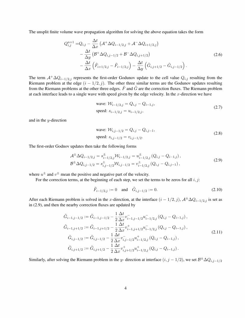
The unsplit finite volume wave propagation algorithm for solving the above equation takes the form

Qn+1i,j =Qi,j −

∆t∆x

(A+∆Qi−1/2,j +A−∆Qi+1/2,j

)− ∆t

∆y(B+∆Qi,j−1/2 + B−∆Qi,j+1/2

)− ∆t

∆x

(Fi+1/2,j − Fi−1/2,j

)− ∆t

∆y

(Gi,j+1/2 − Gi,j−1/2

).

(2.6)

The term A+∆Qi−1/2,j represents the first-order Godunov update to the cell value Qi,j resulting from theRiemann problem at the edge (i − 1/2, j). The other three similar terms are the Godunov updates resultingfrom the Riemann problems at the other three edges. F and G are the correction fluxes. The Riemann problemat each interface leads to a single wave with speed given by the edge velocity. In the x-direction we have

wave: Wi−1/2,j = Qi,j −Qi−1,j ,

speed: si−1/2,j = ui−1/2,j ,(2.7)

and in the y-direction

wave: Wi,j−1/2 = Qi,j −Qi,j−1,

speed: si,j−1/2 = vi,j−1/2.(2.8)

The first-order Godnov updates then take the following forms

A±∆Qi−1/2,j = s±i−1/2,jWi−1/2,j = u±i−1/2,j (Qi,j −Qi−1,j) ,

B±∆Qi,j−1/2 = s±i,j−1/2Wi,j−1/2 = v±i−1/2,j (Qi,j −Qi,j−1) ,(2.9)

where u± and v± mean the positive and negative part of the velocity.For the correction terms, at the beginning of each step, we set the terms to be zeros for all i, j:

Fi−1/2,j := 0 and Gi,j−1/2 := 0. (2.10)

After each Riemann problem is solved in the x-direction, at the interface (i − 1/2, j), A±∆Qi−1/2,j is set asin (2.9), and then the nearby correction fluxes are updated by

Gi−1,j−1/2 := Gi−1,j−1/2 −12

∆t∆x

v−i−1,j−1/2u−i−1/2,j (Qi,j −Qi−1,j) ,

Gi−1,j+1/2 := Gi−1,j+1/2 −12

∆t∆x

v+i−1,j+1/2u

−i−1/2,j (Qi,j −Qi−1,j) ,

Gi,j−1/2 := Gi,j−1/2 −12

∆t∆x

v−i,j−1/2u+i−1/2,j (Qi,j −Qi−1,j) ,

Gi,j+1/2 := Gi,j+1/2 −12

∆t∆x

v+i,j+1/2u

+i−1/2,j (Qi,j −Qi−1,j) .

(2.11)

Similarly, after solving the Riemann problem in the y- direction at interface (i, j − 1/2), we set B±∆Qi,j−1/2

4

as in (2.9) and then update the nearby fluxes by

Fi−1/2,j−1 := Fi−1/2,j−1 −12

∆t∆y

u−i−1/2,j−1v−i,j−1/2 (Qi,j −Qi,j−1) ,

Fi+1/2,j−1 := Fi+1/2,j−1 −12

∆t∆y

u+i+1/2,j−1v

−i,j−1/2 (Qi,j −Qi,j−1) ,

Fi−1/2,j := Fi−1/2,j −12

∆t∆y

u−i−1/2,jv+i,j−1/2 (Qi,j −Qi,j−1) ,

Fi+1/2,j := Fi+1/2,j −12

∆t∆y

u+i+1/2,jv

+i,j1/2 (Qi,j −Qi,j−1) .

(2.12)

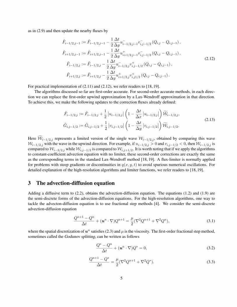
For practical implementation of (2.11) and (2.12), we refer readers to [18, 19].The algorithms discussed so far are first-order accurate. For second-order accurate methods, in each direc-

tion we can replace the first-order upwind approximation by a Lax-Wendroff approximation in that direction.To achieve this, we make the following updates to the correction fluxes already defined:

Fi−1/2,j := Fi−1/2,j +12

∣∣ui−1/2,j

∣∣ (1− ∆t∆x

∣∣ui−1/2,j

∣∣) Wi−1/2,j ,

Gi,j−1/2 := Gi,j−1/2 +12

∣∣vi,j−1/2

∣∣ (1− ∆t∆y

∣∣vi,j−1/2

∣∣) Wi,j−1/2.

(2.13)

Here Wi−1/2,j represents a limited version of the single wave Wi−1/2,j , obtained by comparing this waveWi−1/2,j with the wave in the upwind direction. For example, if ui−1/2,j > 0 and vi,j−1/2 < 0, thenWi−1/2,j iscompared toWi−3/2,j whileWi,j−1/2 is compared toWi,j+1/2. It is worth noting that if we apply the algorithmsto constant-coefficient advection equation with no limiter, these second-order corrections are exactly the sameas the corresponding terms in the standard Lax-Wendroff method [18, 19]. A flux-limiter is normally appliedfor problems with steep gradients or discontinuities in q(x, y, t) to avoid spurious numerical oscillations. Fordetailed explanation of the high-resolution algorithms and limiter functions, we refer readers to [18, 19].

3 The advection-diffusion equation

Adding a diffusive term to (2.2), obtains the advection-diffusion equation. The equations (1.2) and (1.9) arethe semi-discrete forms of the advection-diffusion equations. For the high-resolution algorithms, one way totackle the advecton-diffusion equation is to use fractional step methods [4]. We consider the semi-discreteadvection-diffusion equation

Qn+1 −Qn

∆t+ (un · ∇)Qn+1 =

µ

2(∇2Qn+1 +∇2Qn), (3.1)

where the spatial discretization ofun satisfies (2.3) and µ is the viscosity. The first-order fractional step method,sometimes called the Godunov splitting, can be written as follows

Q∗ −Qn

∆t+ (un · ∇)Q∗ = 0, (3.2)

Qn+1 −Q∗

∆t=µ

2(∇2Qn+1 +∇2Q∗). (3.3)

5

We first compute Q∗ in (3.2) using the high-resolution method described in the previous section. Equation(3.3) is a Crank-Nicolson discretization for the diffusion. It results in a Helmholtz type equation. This splittingmethod is only first-order accurate. Using the same notation, we can write a formally second-order method, theStrang splitting, as follows

Q∗ −Qn

∆t/2=µ

2(∇2Q∗ +∇2Qn), (3.4)

Q∗∗ −Q∗

∆t+ (un · ∇)Q∗∗ = 0, (3.5)

Qn+1 −Q∗∗

∆t/2=µ

2(∇2Qn+1 +∇2Q∗∗). (3.6)

In order to reduce numerical diffusion and computational cost, (3.4) from one step and (3.6) from the followingstep can be combined into a single step of length ∆t. By doing so, Strang splitting uses ∆t/2 only in the firstand last time step. In between, Strang splitting is identical to Godunov splitting. In practice (see [4]), one canobtain better than first-order accuracy using Godunov splitting.

4 A projection method: conservative algorithm approach

We begin this section with the definitions of our discrete divergence and discrete gradient operators. In orderto use the high-resolution algorithms from Section 2, the discrete values of the cell interface velocities have tosatisfy(2.3). In two dimension space, let

ui±1/2,j±1/2 = (ui±1/2,j , vi,j±1/2)

denote the horizontal and vertical components of the discrete velocity field at the edges of the (i, j) cell Ci,j

and letU i,j = (Ui,j , Vi,j)

denote the approximation to the cell average

U i,j ≈1

∆x∆y

∫Ci,j

U(x, y, t) dx dy.

Assuming that φ is a scalar function, we consider a staggered grid as shown in Figure 4.1 and define the discretegradient and divergence operators as follows

(Du)i,j =ui+1/2,j − ui−1/2,j

∆x+vi,j+1/2 − vi,j−1/2

∆y, (4.1)

(Gφ)i,j = (φi,j − φi−1,j

∆x,φi,j − φi,j−1

∆y), (4.2)

(DU)i,j =Ui+1,j − Ui−1,j

2∆x+Vi,j+1 − Vi,j−1

2∆y, (4.3)

(Gφ)i,j = (φi+1,j − φi−1,j

2∆x,φi,j+1 − φi,j−1

2∆y). (4.4)

Using these operators, we introduce the algorithm of the new projection method in two-dimensional space. LetU be the divergence-free velocity field with respect to the continuous divergence operator. U i,j is the discrete

6

PSfrag replacements

vi,j+1/2

ui−1/2,j

vi,j−1/2

ui+1/2,j

Ui,j

φi,j

Vi,j

Figure 3.1: Cell variables of the projection method .

denote the approximation to the cell average

U i,j ≈1

"x " y

∫

Ci,j

U(x, y, t) dx dy.

Assuming that φ is a scalar function, we consider a staggered grid as shown in Figure 3.1 and define the discretegradient and divergence operators as follows

(Du)i,j =ui+1/2,j − ui−1/2,j

"x+

vi,j+1/2 − vi,j−1/2

"y(3.1)

(Gφ)i,j = (φi,j − φi−1,j

"x,φi,j − φi,j−1

"y) (3.2)

(DU)i,j =Ui+1,j − Ui−1,j

2 " x+

Vi,j+1 − Vi,j−1

2 " y(3.3)

(Gφ)i,j = (φi+1,j − φi−1,j

2 " x,φi,j+1 − φi,j−1

2 " y). (3.4)

Using these operators, we introduce the algorithm of the new projection method in two-dimensional space. LetU be the divergence-free velocity field with respect to the continuous divergence operator. U i,j is the discretevalue of U at the cell center of Ci,j . We find the discrete edge velocity by taking the average the cell-centeredvalues. For example, the left edge value of cell Ci,j is

ui−1/2,j =1

2(Ui−1,j + Ui,j) (3.5)

and the bottom edge value isvi,j−1/2 =

1

2(V,j−1 + Vi,j). (3.6)

If the edge values (3.5) and (3.6) satisfy (1.5) initially, the edge velocities are discrete divergence free withrespect to the operator (3.1). Otherwise, we need to apply one projection step so that (1.5) is satisfied. We willexplain the projection step in Step P2.The algorithm then takes the following form.

4

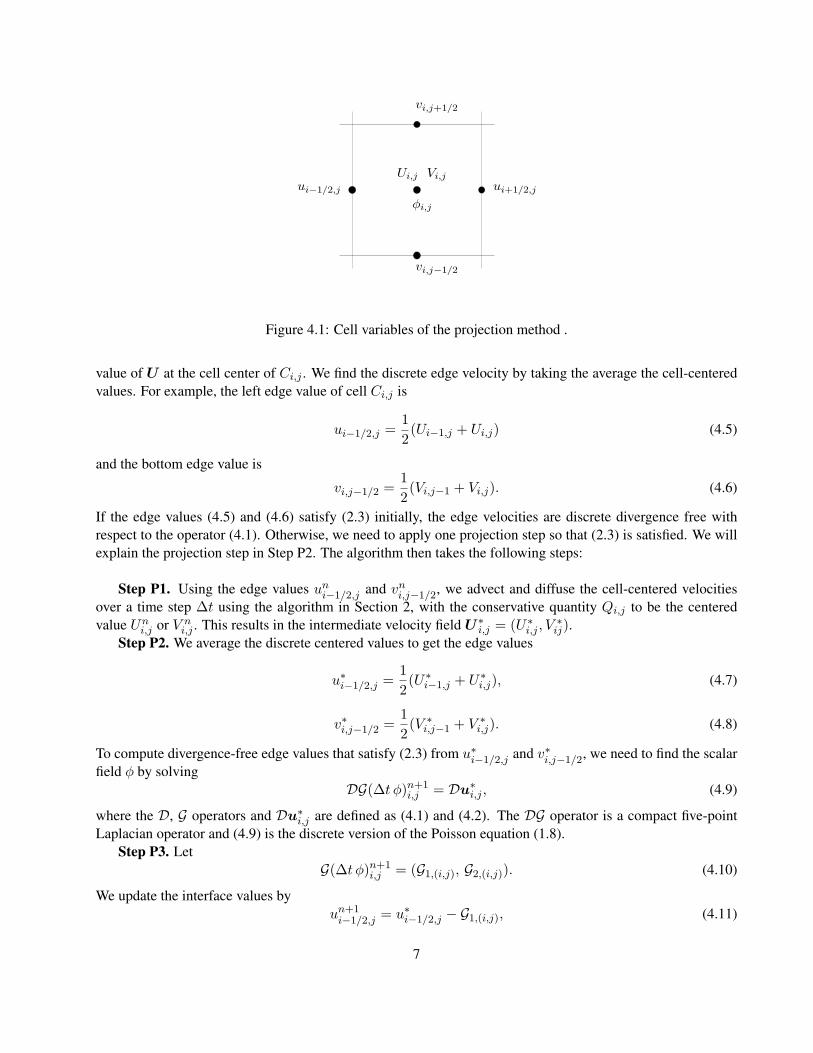
Figure 4.1: Cell variables of the projection method .

value of U at the cell center of Ci,j . We find the discrete edge velocity by taking the average the cell-centeredvalues. For example, the left edge value of cell Ci,j is

ui−1/2,j =12

(Ui−1,j + Ui,j) (4.5)

and the bottom edge value is

vi,j−1/2 =12

(Vi,j−1 + Vi,j). (4.6)

If the edge values (4.5) and (4.6) satisfy (2.3) initially, the edge velocities are discrete divergence free withrespect to the operator (4.1). Otherwise, we need to apply one projection step so that (2.3) is satisfied. We willexplain the projection step in Step P2. The algorithm then takes the following steps:

Step P1. Using the edge values uni−1/2,j and vn

i,j−1/2, we advect and diffuse the cell-centered velocitiesover a time step ∆t using the algorithm in Section 2, with the conservative quantity Qi,j to be the centeredvalue Un

i,j or V ni,j . This results in the intermediate velocity field U∗i,j = (U∗i,j , V

∗ij).

Step P2. We average the discrete centered values to get the edge values

u∗i−1/2,j =12

(U∗i−1,j + U∗i,j), (4.7)

v∗i,j−1/2 =12

(V ∗i,j−1 + V ∗i,j). (4.8)

To compute divergence-free edge values that satisfy (2.3) from u∗i−1/2,j and v∗i,j−1/2, we need to find the scalarfield φ by solving

DG(∆t φ)n+1i,j = Du∗i,j , (4.9)

where the D, G operators and Du∗i,j are defined as (4.1) and (4.2). The DG operator is a compact five-pointLaplacian operator and (4.9) is the discrete version of the Poisson equation (1.8).

Step P3. LetG(∆t φ)n+1

i,j = (G1,(i,j), G2,(i,j)). (4.10)

We update the interface values byun+1

i−1/2,j = u∗i−1/2,j − G1,(i,j), (4.11)

7

vn+1i,j−1/2 = v∗i,j−1/2 − G2,(i,j), (4.12)

so that Dun+1i,j = 0 and (2.3) is satisfied.

Step P4. LetG0(∆t φ)n+1

i,j = (G01,(i,j), G

02,(i,j)). (4.13)

We update the cell-centered values byUn+1

i,j = U∗i,j − G01,(i,j), (4.14)

V n+1i,j = V ∗i,j − G0

2,(i,j). (4.15)

The exactly divergence-free edge values are obtained by subtracting G1,(i,j) and G2,(i,j) from the intermediateedge velocities. It is easy to show

G01,(i,j) =

12

(G1,(i,j) + G1,(i+1,j)), (4.16)

G02,(i,j) =

12

(G2,(i,j) + G2,(i,j+1)), (4.17)

by the definition of equations (4.2) and (4.4). So it is natural to update cell-centered values Un+1 using (4.14)and (4.15). One can expect Un+1 to be divergence free up to second order, since the edge values are exactlydivergence free. This completes one time step. Go to Step P1 for the next time step.

4.1 Discussion

1. The boundary conditions used for the elliptic equation (4.9) are the Neumann boundary conditions dis-cussed in [10].

2. From (4.1), (4.3), (4.7), and (4.8), it is easy to show

Du∗i,j = D0U∗i,j . (4.18)

Combining (4.9) and (4.18) givesDG(∆t φ)n+1

i,j = D0U∗i,j . (4.19)

If we apply the operator D0 on (4.14) and (4.15) and compare the resulting equation with (4.19), we seethat the cell-centeredUn+1 is not discrete divergence free with respect to the discrete divergence operatorD0, but it is divergence free up to second order. Minion [21] used a similar approach in his BCG versionof adaptive projection methods to avoid the decoupled stencil arising from the projection step.

3. Although in Step P1 we do not need the pressure p to advance the velocity, we can obtain the pressurepn+1 from (1.7) within each time step. The projection method stated in the previous section is parallel tothe finite difference scheme of Kim and Moin.

4. If we update the pressure gradient ∇pn+1/2 using (1.11) and add ∇pn−1/2 in the advection-diffusionequation in Step P1, the modified projection method is parallel to the pressure-correction (BCG) scheme.The term∇pn−1/2 in the advection-diffusion equation is treated as an external force and is solved togetherwith the diffusive term using the fractional-step method in Section 3.

8

5. Since the high-resolution method used in Step P1 to advect the intermediate velocity field is explicit, aCFL condition must be imposed to ensure stability. The method requires

maxi,j

(∆t∆x|ui−1/2,j |,

∆t∆y|vi,j−1/2|) 6 1. (4.20)

6. It was pointed out in [20] that if we use an interpolant, such as the arithmetic average, to interpolate thedivergence free cell-edge values back to the cell centers, instead of using the approximate projection,i.e. (4.14) & (4.15), it will introduce a diffusive term into the discretized equation which resembles aone-dimensional Laplacian with a magnitude which scales like the grid size h. Even if higher orderinterpolation is used, a similar diffusive term will result, making this approach undesirable for flows athigh Reynolds numbers.

7. The authors in [1] indicated that 76% of the computational time for their projection method is usedto solve the elliptic potential equation (the projection linear algebra). While the high-resolution wavepropagation algorithms are robust for treating flows at high Reynolds numbers, potentially they could bemore expensive than traditional finite difference methods, due to the cost of solving Riemann problemat each interface, but we expect that this is not the dominant cost for the proposed projection methods.Since the computational cost heavily depends on the choice of elliptic solvers for projection methods, weexpect that the efficiency of the proposed algorithms should be at least comparable to traditional finitedifference methods.

5 A projection method for variable-density flows

In this section, we extend the high-resolution algorithms for solving the variable-density incompressible Navier-Stokes equations. Only a slight modification of the projection operator is required. We consider the unsteadyincompressible Navier-Stokes equations for flows with finite-amplitude density variation. Conservation of massis described by an advection equation. We write the system of equations as follows

ut + (u · ∇)u =1ρ

(∇ · µ(∇u+ (∇u)T )−∇p+ F ),

ρt + (u · ∇)ρ = 0,∇ · u = 0,

(5.1)

where ρ is the density and µ is the viscosity that is allowed to depend on density. Function F is an externalforce while u and p are the velocity and hydrodynamic pressure respectively. In two-dimensional space, letu = (u, v) and q = (u, v, ρ) = (u, ρ). For simplicity, we assume µ is a constant. Again for simplicity, weconsider the Dirichlet boundary conditions. The projection method based on the high-resolution conservativealgorithm for the above system can be stated as follows.

Step V1. Use the centered valuesQn = (Un, V n, ρn) and edge valuesun = (un, vn) to solve the advectionequation

Q−Qn

∆t+ un · ∇Q = 0. (5.2)

This is solved on a finite-volume grid using the explicit second-order high-resolution algorithm developed byLeVeque [19]. The resulting solution isQ† = (U †, ρ†) = (U †, V †, ρ†).

9

Step V2. Use a Crank-Nicolson discretization for the diffusion

U∗ −U †

∆t=

µ

2ρ†(∇2U∗ +∇2U † + F ). (5.3)

This gives the intermediate velocity U∗ at cell center.Step V3. Obtain the edge velocity un+1 by

un+1 = u∗ − 1ρG(∆tφn+1), (5.4)

where u∗ is the average of the adjacent U∗ and ρ is the average of the adjacent ρ†.The update (5.4) requires the value φn+1, which can be obtained by solving a discrete Poisson problem:Taking the discrete divergence of (5.4) and using the fact that we want Dun+1 = 0, we obtain the variable-

coefficient Poisson problem

D(

1ρGφn+1

)=

1∆tDu∗. (5.5)

This is solved on a finite-volume grid using the explicit second-order high-resolution algorithm from CLAW-PACK. The resulting solution isQ† = (U †, ρ†) = (U †, V †, ρ†).Step V2. Use a Crank-Nicolson discretization for the diffusion

U∗ − U †

"t=

µ

2ρ†(∇2U∗ + ∇2U † + F ). (4.3)

This gives the intermediate velocity U ∗ at cell center.Step V3. Obtain the edge velocity un+1 by

un+1 = u∗ −1

ρG("tφn+1), (4.4)

where u∗ is the average of the adjacent U ∗ and ρ is the average of the adjacent ρ†.The update (4.4) requires the value φn+1, which can be obtained by solving a discrete Poisson problem:Taking the discrete divergence of (4.4) and using the fact that we want Dun+1 = 0, we obtain the variable-

coefficient Poisson problemD

(

1

ρGφn+1

)

=1

"tDu∗ (4.5)

PSfrag replacements

ρi,j+1/2

ρi−1/2,j

ρi,j−1/2

ρi+1/2,j

φi,j

Figure 4.1: Staggered grid for the Poisson problem with variant coefficients

Consider the staggered grid shown in Figure 4.1. If we denote

βi−1/2,j =1

ρi−1/2,j, (4.6)

then a finite difference discretization for (4.5) is

φi+1,j βi+1/2,j − φi,j(βi+1/2,j + βi−1/2,j) + φi−1,j βi−1/2,j

("x)2+

φi,j+1 βi,j+1/2 − φi,j(βi,j+1/2 + βi,j−1/2) + φi,j−1 βi,j−1/2

("y)2=

1

"t

(

u∗i+1,j − 2u∗

i,j + u∗i−1,j

("x)2+

v∗i,j+1 − 2v∗i,j + v∗i,j−1

("y)2

)

.

(4.7)

7

Figure 5.1: Staggered grid for the Poisson problem with variant coefficients

Consider the staggered grid shown in Figure 5.1. If we denote

βi−1/2,j =1

ρi−1/2,j, (5.6)

then a finite difference discretization for (5.5) is

φi+1,j βi+1/2,j − φi,j(βi+1/2,j + βi−1/2,j) + φi−1,j βi−1/2,j

(∆x)2+

φi,j+1 βi,j+1/2 − φi,j(βi,j+1/2 + βi,j−1/2) + φi,j−1 βi,j−1/2

(∆y)2=

1∆t

(u∗i+1,j − 2u∗i,j + u∗i−1,j

(∆x)2+v∗i,j+1 − 2v∗i,j + v∗i,j−1

(∆y)2

).

(5.7)

The resulting linear system from (5.7) isAφ = f , (5.8)

10

where the coefficient matrixA is symmetric and positive definite [12].Step V4. In the final step, we update the cell-centered values by

Un+1 = U∗ − ∆t2

(1

ρi−1/2,j(φi,j − φi−1,j) +

1ρi+1/2,j

(φi+1,j − φi,j)), (5.9)

V n+1 = V ∗ − ∆t2

(1

ρi,j−1/2(φi,j − φi,j−1) +

1ρi,j−1/2

(φi,j+1 − φi,j)), (5.10)

and set ρn+1 = ρ†. This completes one time step. Go to Step V1 for next time step.It is worth noting that if the density ρ ≡ 1 is constant, then the algorithm is identical to the projection

method in Section 4. We remark that the proposed algorithm becomes unstable if the density ratio is over athreshold (between 100 and 200).

6 A high-resolution method for the Boussinesq flow

We consider the convection of a Boussinesq fluid in a two-dimension rectangular cavity on x-z plane. The flowis governed by the dimensionless Boussinesq equations [11]:

Pr−1 [ut + (u · ∇u)u ] = −∇p+∇2u+RaTez,

Tt + (u · ∇)T = ∇2T,

∇ · u = 0,u = 0 on z = Za and z = Zb,

T = Ta on z = Za, T = Tb on z = Zb,

(6.1)

where T is the temperature, Pr the Prantal number, and Ra the Rayleigh number. Here ez is the unit vector inthe vertical direction. The dimensionless parameter Ra is given by

Ra =α g (Tb − Ta) d3

ν κ, (6.2)

where α is the thermal expansion coefficient, Ta and Tb the temperatures of the top and bottom plates, d =Za − Zb the height of the cavity, g the gravity acceleration, ν the kinematic viscosity, and κ the thermaldiffusion. The other parameter Pr is given by

Pr =ν

χ, (6.3)

where χ is the thermal conductivity.The Boussinesq equation is a good approximation for studying Rayleigh-Benard convection, in which a

viscous fluid in a cavity is heated from the bottom plate and the top plate is maintained at a lower temperature.When the temperature between the top and bottom plates is a linear function of the height of the cavity and theinitial velocity is zero everywhere, the linear stability theorem shows that a static solution exists to the problem(6.1) [5]. Increasing the temperature of the hot plate until the Rayleigh number is above a critical value,Rac, the static solution becomes unstable to any small disturbance. The system then turns from conduction toconvection. Some properties of non-linear thermal convection are analyzed and compared with experimentalobservations in the paper by Busse [3] .

11

Similar to Section 5, in two-dimensional space, let u = (u, v) and define q = (u, v, T ) = (u, T ). Thehigh-resolution algorithm for the Boussinesq approximation can be described in the following:

Step B1. Use the centered values Qn = (Un, V n, Tn) and edge values un = (un, vn) to solve theadvection equation

Q−Qn

∆t+ un · ∇Q = 0. (6.4)

Similar to Step V1, this is solved by the high-resolution algorithm developed in [19], and the resulting solutionisQ† = (U †, T †) = (U †, V †, T †).

Step B2. Use a Crank-Nicolson discretization for the thermal diffusion and the diffusive term.

T n+1 − T †

∆t=

12

(∇2T n+1 +∇2T †), (6.5)

andU∗ −U †

∆t=Pr

2(∇2U∗ +∇2U †) + PrRaTn+1 ez. (6.6)

Both Step B1 and Step B2 are subject to boundary conditions accordingly.Step B3. Obtain the edge velocity un+1 by

un+1 = u∗ − Pr G(∆tφn+1), (6.7)

and update the centered velocityUn+1 = U∗ − Pr G0(∆tφn+1). (6.8)

Again u∗ is the average of the adjacent U∗, and φn+1 is obtained by solving (4.9) with Neumann boundarycondition (1.8). G and G0 are defined as before.

7 Numerical results

In this section, we present several examples that validate the convergence properties of the methods developedpreviously. We demonstrate the performance of the methods via numerical results and show their potential forsolving more realistic problems.

Example 7.1 The first example is the stationary Taylor’s vortices [28]. We use this example to demonstratethe rate of convergence of our methods. We consider a stationary inviscid flow to show that our method issuitable for fluids at high Reynolds numbers.

In the absence of viscosity, an exact steady solution of the incompressible Navier-Stokes equations in aperiodic unit square is given by

u(x, y) = −cos(2mπx)sin(2mπy), (7.1)

v(x, y) = sin(2mπx)cos(2mπy), (7.2)

where m is some integer. We consider the case m = 2. Using (7.1) and (7.2) as initial data, we show the resultsfor time t = 1. Ideally the solution would be unchanged. Table 7.1 shows the l2 and infinity norms for the errorof the u-component velocity. The l2 norm is defined by

12

‖ u ‖2=

√∑|u|2

mxmy, (7.3)

where mx and my are the numbers of grid cells in x and y directions, respectively.The CFL number is fixed at 0.9. It appears that the method is formally second-order accurate. We show that

the method used to compute the results has the same formulation as the BCG scheme. The algorithm is stablefor 0 < γ ≤ 2/3. We choose γ = 2/3 and no limiter is used for this simulation. A fixed time step ∆t = 0.01is used for the 32 × 32 grid. The time step is reduced to a half when the grid size is reduced to a half. Theprojection method that uses the formulation resembling Kim and Moin’s scheme has similar results.

Table 7.1: Convergence rate, u-component velocity.

32×32 rate 64×64 rate 128×128 rate 256×256‖ u− uexact ‖2 2.066E-3 2.69 3.196E-3 2.83 4.506E-4 2.74 6.724E-5‖ u− uexact ‖∞ 4.526E-2 2.73 6.825E-3 2.84 9.534E-4 2.64 1.531E-4

0 0.5 10

0.5

1

(a) t=0

0 0.5 10

0.5

1

(b) t=1

Figure 7.1: u-component velocity contour of the Taylor’s vortex. 20 contour lines with equally spaced valuesbetween ± 1.

Figure 7.1 shows the u-component velocity contours. The computation is done using a 256×256 grid. Theinterval between plotted contour lines is 0.1. There are 20 contour lines with equally spaced values between± 1.

Example 7.2. The second example is the bench-mark lid-driven cavity flow, which has been intensivelystudied. It is a hard test problem, particularly at high Reynolds numbers, due to the two singular points atthe upper corners. In the paper by Gresho and Chan [13], several finite difference schemes based on projec-tion methods were tested and compared with the stream-function-vorticity formulation [6]. They all deliveredweaker flows than desired. Compared with the results by Gresho and Chan [13], our methods give a strongerprimary vortex. For Fig 7.2, we use a uniform 256 × 256 grid and the Reynolds number is Re=5000. The CFL

13

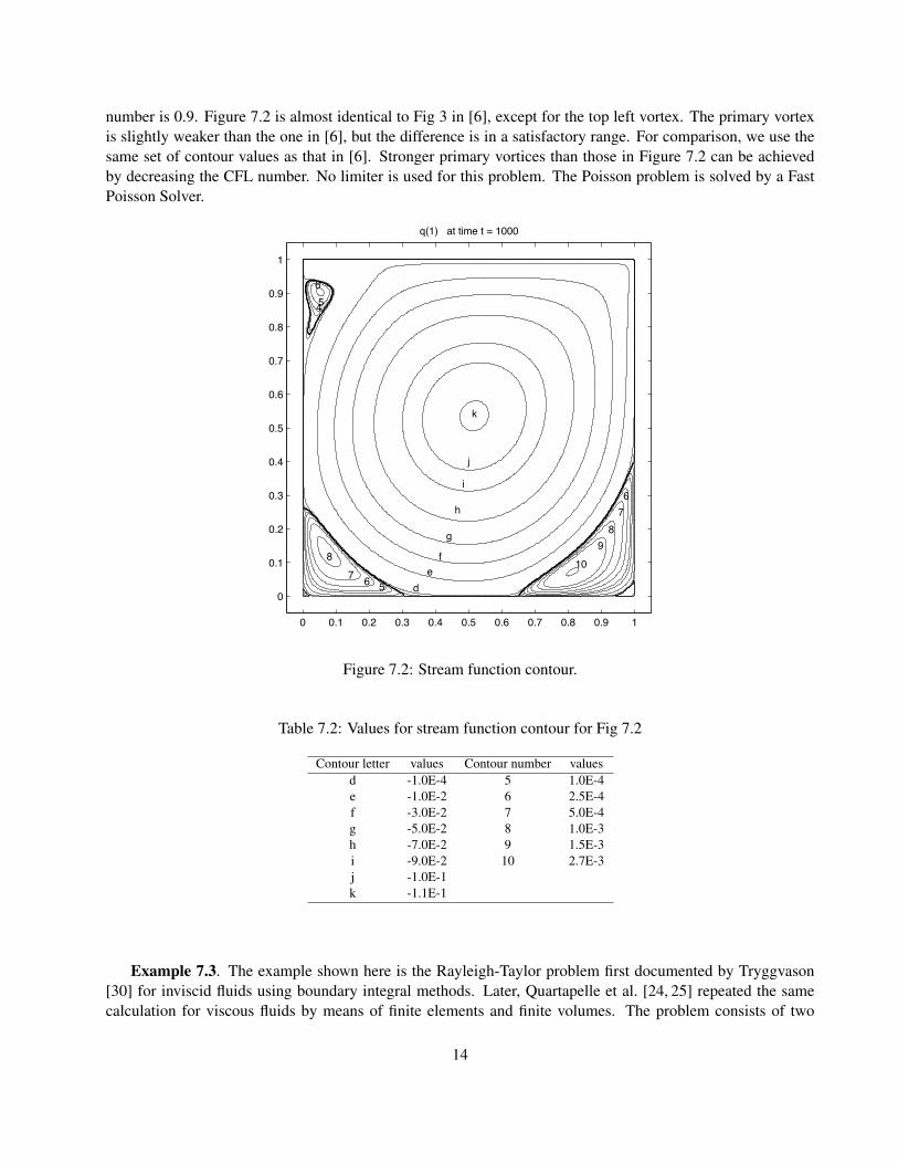
number is 0.9. Figure 7.2 is almost identical to Fig 3 in [6], except for the top left vortex. The primary vortexis slightly weaker than the one in [6], but the difference is in a satisfactory range. For comparison, we use thesame set of contour values as that in [6]. Stronger primary vortices than those in Figure 7.2 can be achievedby decreasing the CFL number. No limiter is used for this problem. The Poisson problem is solved by a FastPoisson Solver.

0 0.1 0.2 0.3 0.4 0.5 0.6 0.7 0.8 0.9 1

0

0.1

0.2

0.3

0.4

0.5

0.6

0.7

0.8

0.9

1

q(1) at time t = 1000

8

76

5

10

9

8

7

6

54

6

d

e

f

g

h

i

j

k

Figure 7.2: Stream function contour.

Table 7.2: Values for stream function contour for Fig 7.2

Contour letter values Contour number valuesd -1.0E-4 5 1.0E-4e -1.0E-2 6 2.5E-4f -3.0E-2 7 5.0E-4g -5.0E-2 8 1.0E-3h -7.0E-2 9 1.5E-3i -9.0E-2 10 2.7E-3j -1.0E-1k -1.1E-1

Example 7.3. The example shown here is the Rayleigh-Taylor problem first documented by Tryggvason[30] for inviscid fluids using boundary integral methods. Later, Quartapelle et al. [24, 25] repeated the samecalculation for viscous fluids by means of finite elements and finite volumes. The problem consists of two

14

layers of fluid initially at rest in a gravity field. A heavy fluid is put on top of the light fluid, and the heavy fluidaccelerates into the light fluid under the action of gravity. The domain for the fluid is (−d/2, d/2) × (2d, 2d),and the initial position of the interface of the layers is given by

η(x) = −0.1 d cos(

2πxd

).

The density ratio of heavy fluid to light fluid is 3, which makes the Atwood number 0.5. The Atwoodnumber At is defined as At = (ρmax − ρmin)/(ρmax + ρmin). In order to compare this with the resultsin [24, 25], we regularize the transition between the two fluids by a tanh profile:

ρ(x, y, t = 0)ρmin

= 2 + tanh(y − η(x)

0.01d

).

The governing equations are made dimensionless by using the following references: ρmin for density, d forlength, d1/2g−1/2 for time, where g is the magnitude of gravity field, and g for gravity. The reference velocityis d1/2g1/2, and the Reynolds number is defined by Re = ρmind

2/3g1/2/µ. No-slip boundary conditions areapplied to the top and bottom walls while periodic boundary conditions are imposed on the two vertical sides.The output time t is in the scale of Tryggvason. t is related to our dimensionless time scale t by t = t

√At.

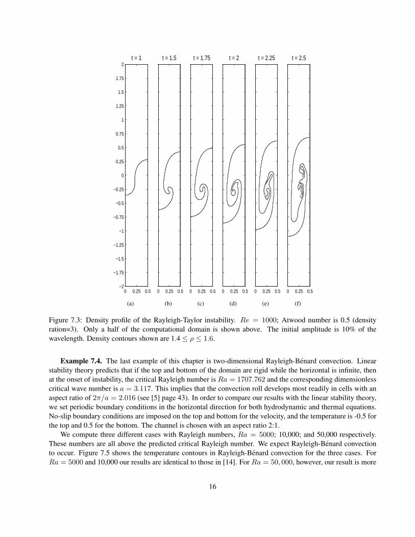
Figure 7.3 shows the results for Re = 1000 using 128× 512 cells. In order to compare the positions of thefalling jet and the uprising bubble with those in [24,25], we only plot half of the domain, which is composed of32768 cells. Both the positions and the development of the roll-up structure of our results are similar to thosein [24, 25], for which 30189 P2 nodes are used. There are no noticeable differences between the two sets ofresults, except that our results reveal more detailed roll-up structure. It is worth noting that in [24, 25], a rathersmall time step ∆t = 5 × 10−4 is chosen for the spatial discretization. Our CFL number is fixed at 0.9 andtime step can be chosen by ∆t ∼ 6× 10−3. A monotonized centered (MC) limiter is used for both velocity anddensity field, and the linear system (5.8) is solved by an incomplete Cholesky conjugate-gradient method.

Based on their results, the authors in [24, 25] indicate that obtaining an accurate and detailed prediction ofthe large-time phenomena for the viscous Rayleigh-Taylor instability at high Reynolds numbers is very difficult.They report that for t ≥ 1.5 and Re ≥ 5000, the numerical results of this problem are not only sensitive to thegrid resolutions but also to the numerical methods used to compute those results. The solutions computed byeither the finite element method or the finite volume method for Reynolds numberRe = 5000 are very differentfrom the inviscid one reported in [30] at or beyond t = 1.5. The solutions of the two methods are also differentfrom each other. The authors speculate that this problem has no smooth inviscid solution for large time, basedon Birkhoff’s conjecture. Birkhoff’s conjecture says that the initial-value problem for inviscid stratified flowsmight be ill-posed, as a consequence of the fact that the growth rate of an infinitely small unstable wave isproportional to the square root of its wave number. Figure 7.4 shows the solutions computed by our algorithmfor Re = 5000. (a) uses the MC limiter and (b) uses the superbee limiter to eliminate the numerical oscillationdue to the density discontinuity. In contrast to the results reported in [24, 25], our results are compatible withthose in [30] before t = 2, especially for the solution using the MC limiter. However, after t = 2 we didobserve that the results are sensitive to the limiters used for the computation. We conclude that it is hard to givean accurate and detailed prediction of the large-time phenomena for this problem at high Reynolds numbers, asthe authors in [24, 25] indicated.

Because the above example does not consider surface tension that is a curvature-dependent effect, no inter-face tracking scheme is required. When the surface tension is taken into account, different approaches such asthe volume of fluid method [22], the front-tracking algorithm [23], or the immersed interface method [17] willbe needed to do this work.

15

0 0.25 0.5−2

−1.75

−1.5

−1.25

−1

−0.75

−0.5

−0.25

0

0.25

0.5

0.75

1

1.25

1.5

1.75

2t = 1

(a)

0 0.25 0.5

t = 1.5

(b)

0 0.25 0.5

t = 1.75

(c)

0 0.25 0.5

t = 2

(d)

0 0.25 0.5

t = 2.25

(e)

0 0.25 0.5

t = 2.5

(f)

Figure 7.3: Density profile of the Rayleigh-Taylor instability. Re = 1000; Atwood number is 0.5 (densityration=3). Only a half of the computational domain is shown above. The initial amplitude is 10% of thewavelength. Density contours shown are 1.4 ≤ ρ ≤ 1.6.

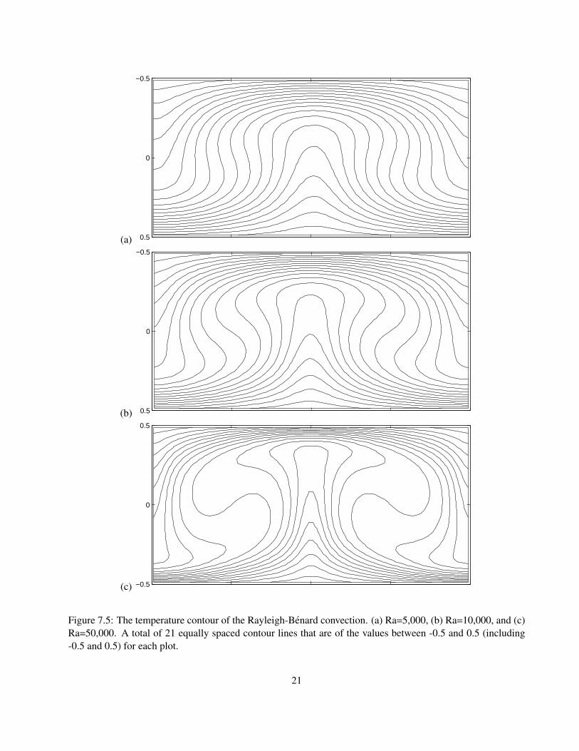
Example 7.4. The last example of this chapter is two-dimensional Rayleigh-Benard convection. Linearstability theory predicts that if the top and bottom of the domain are rigid while the horizontal is infinite, thenat the onset of instability, the critical Rayleigh number is Ra = 1707.762 and the corresponding dimensionlesscritical wave number is a = 3.117. This implies that the convection roll develops most readily in cells with anaspect ratio of 2π/a = 2.016 (see [5] page 43). In order to compare our results with the linear stability theory,we set periodic boundary conditions in the horizontal direction for both hydrodynamic and thermal equations.No-slip boundary conditions are imposed on the top and bottom for the velocity, and the temperature is -0.5 forthe top and 0.5 for the bottom. The channel is chosen with an aspect ratio 2:1.

We compute three different cases with Rayleigh numbers, Ra = 5000; 10,000; and 50,000 respectively.These numbers are all above the predicted critical Rayleigh number. We expect Rayleigh-Benard convectionto occur. Figure 7.5 shows the temperature contours in Rayleigh-Benard convection for the three cases. ForRa = 5000 and 10,000 our results are identical to those in [14]. For Ra = 50, 000, however, our result is more

16

symmetric between hot and cold fluids. For comparison, our computational grid is 80 × 40, and the Prantalnumber is Pr = 0.71. Both are the same as [14].

8 Conclusion

We presented a class of high-resolution algorithms for incompressible flows that prove to be robust and suit-able for incompressible flows at high Reynolds numbers. The implementation of the proposed algorithms forvariable-density flows is straightforward, and the strength of the algorithms is illustrated through problemslike Rayleigh-Taylor instability and the Boussinesq equations for Rayleigh-Benard convection. Although onlytwo-dimensional regular-geometry problems are present in this study, extension of the algorithms to three di-mensions with complex geometry is possible, because the wave-propagation algorithms on curved manifoldhas been introduced in [26] and three-dimensional wave-progation algorithms are available though [16].

9 Acknowledgment

This work is partially supported by NSF through the Grant DMS-0610149.

References

[1] J. B. Bell, P. Colella and H. M. Glaz. A second-order projection method for the incompressible Navier-Stokes equations. J. Comput. Phys., 85 (1989) 257-283.

[2] D. Brown, R. Cortez, and M. L. Minion. Accurate projection methods for the incompressible Navier-Stokesequations. J. Comput. Phys., 168, (2001) 464-499.

[3] F. H. Busse. Non-linear propertites of thermal convection. Report on the Progress in Physics, 41 (1978)1929-1967.

[4] D. Calhoun and R. J. LeVeque. A Cartesian grid finite-volume method for the advection-diffusion equationin irregular regions. J. Comput. Phys., 156 (2002) 1-38.

[5] S. Chandrasekhar. Hydrodynamic and Hydrmagnetic. Oxford University Press, 1961.

[6] U. Chia, K. N. Chia and C. T. Shin. High-Re solutions for incompressible flow using the Navier-Stokesequations and a multigrid method. J. Comput. Phys., 48 (1982) 387-411.

[7] A. J. Chorin. Numerical solutionof incompressible flow problems. Studies in Numerical Analysis, 2 (1968)64-71.

[8] A. J. Chorin. Numerical solution of the Navier-Stokes equation. Math. Comp., 22 (1968) 742-762.

[9] A. J. Chorin. On the convergence of discrete approximations to the Navier-Stokes equations. Math. Comp.,22 (1968) 742-762.

[10] W. E and J.-G. Liu. Projection method I: convergence and numerical boundary layers SIAM J. Numer.Anal. , 32 (1995) 1017-1057.

17

[11] A. Y. Gelfgat. Different modes of Rayleigh-Benard instability in two- and three-dimensional rectangularenclosures. J. Comput. Phys., 156 (1999) 300-324.

[12] A. Greenbaum. Iterative methods for solving linear system. Frontiers in applied mathematics. SIAMPublish, 1997.

[13] P. M. Gresho and S. T. Chan. On the theory of semi-implicit projection methods for viscous incompressibleflow and its implementation via a finite element method that also introduces a nearly consistent mass matrix.part II: Implememtation. International Journal for Numerical Methods in Fluids, 11 (1990) 621-659.

[14] X. He, S. Chen and G. D. Doolen. A Novel thermal model for the lattice Boltzmann method in incom-pressible limit. J. Comput. Phys., 146 (1998) 282-300.

[15] J. Kim and P. Moin. Application of a fractional-step method to incompressible Navier-Stokes equations.J. Comput. Phys., 59 (1985) 308-323.

[16] J. O. Langseth and R. J. LeVeque. A wave propagation method for three-dimensional hyperbolic conser-vation laws. J. Comput. Phys., 165 (2000), 126-166.

[17] L. Lee and R.J. LeVeque. An immersed interface method for the incompressible Navier-Stokes equationsSIAM Sci Comp , 25 (2003) 832-856.

[18] R. J. LeVeque. High-resolution conservative algorithms for advection in incompressible flow. SIAM J.Numer. Anal., 33 (1996) 627-665.

[19] R. J. LeVeque. Finite Volume Methods for Hyperbolic Problems. Cambridge Texts in Applied Mathemat-ics, August 26, 2002.

[20] M. L. Minion. Two methods for the study of vortex patch evolution on local refined grids. Ph. D. Thesis,University of California, Berkeley, CA 94720, May 1994.

[21] M. L. Minion. A projection method for locally refined grids. J. Comput. Phys., 127 (1996) 158-178.

[22] E. G. Puckett, A. S. Almgren, J. B. Bell, D. L. Marcus and W. J. Rider A high-order projection method fortracking fluid interfaces in variable density incompressible flows. J. Comput. Phys., 130 (1997) 267-282.

[23] S. Popinet and S. Zaleski. A front-tracking algorithm for accurate representation of surface tension.International Journal for Numerical Methods in Fluids, 30 (1999) 775-793.

[24] J.-L. Guermond and L. Quartapelle A projection FEM for variable density incompressible flows. J.Comput. Phys., 165 (2000) 167-188.

[25] Y. Frigneau and J.-L. Guermond and L. Quartapelle. Approximation of variable density incompressibleflows by means of finite elements and finite volumes. Communications in Numerical Methods in Engineer-ing, 17 (2001) 893-902.

[26] J. A. Rossmanith, D. S. Bale, and R. J. LeVeque. A wave propagation algorithm for hyperbolic systemson curved manifolds. J. Comput. Phys., 199 (2004) 631-662.

[27] J. Shen. On error estimates of some higher order projection and penalty-projection methods for Navier-Stokes equations. Numer. Math., 62 (1992) 49-73.

18

[28] G. I. Taylor. On the decay of vortices in a viscous fluid. Philos. Mag., 46 (1923) 671-674.

[29] R. Temam. Sur l’approximation de la solution des equations de Navier-Stokes par la methode des frac-tionaries II. Arc. Rational Mech. Anal., 33 (1969) 377-385.

[30] G. Tryggvason. Numerical simulations of the Rayleigh-Taylor instability. J. Comput. Phys., 75 (1988)253-282.

[31] J. Van Kan. A second-order accurate pressure-correction scheme for viscous incompressible flow. SIAMJ. Sci. Comput, 7 (1986) 870-891.

19

(a)−0.5 0 0.5

t = 0

−0.5 0 0.5

t = 1

−0.5 0 0.5

t = 1.5

−0.5 0 0.5

t = 1.75

−0.5 0 0.5

t = 2

−0.5 0 0.5

t = 2.25

−0.5 0 0.5

t = 2.5

(b)−0.5 0 0.5

t = 0

−0.5 0 0.5

t = 1

−0.5 0 0.5

t = 1.5

−0.5 0 0.5

t = 1.75

−0.5 0 0.5

t = 2

−0.5 0 0.5

t = 2.25

−0.5 0 0.5

t = 2.5

Figure 7.4: Re=5000; density ratio 3. The grid is 128×512. The interface is shown at times 0, 1, 1.5, 1.75, 2,2.25, and 2.5 using the density contours 1.4 ≤ ρ ≤ 1.6. The initial amplitude is 10% of the wavelength. (a) iscomputed with the MC limiter; (b) is computed with the superbee limiter.

20

(a)

−0.5

0

0.5

(b)

−0.5

0

0.5

(c) −0.5

0

0.5

Figure 7.5: The temperature contour of the Rayleigh-Benard convection. (a) Ra=5,000, (b) Ra=10,000, and (c)Ra=50,000. A total of 21 equally spaced contour lines that are of the values between -0.5 and 0.5 (including-0.5 and 0.5) for each plot.

21