A Charging and Storage Infrastructure Design for Electric Vehicles

A

Charging and Storage Infrastructure Design for Electric Vehicles

MARJAN MOMTAZPOUR and PATRICK BUTLER, Virginia TechM. SHAHRIAR HOSSAIN, University of Texas at El PasoMOHAMMAD C. BOZCHALUI and RATNESH SHARMA, NEC Laboratories America, Inc.NAREN RAMAKRISHNAN, Virginia Tech

Ushered by recent developments in various areas of science and technology, modern energy systems aregoing to be an inevitable part of our societies. Smart grids are one of these modern systems that haveattracted many research activities in recent years. Before utilizing the next generation of smart grids, weshould have a comprehensive understanding of the interdependent energy networks and processes. Next-generation energy systems networks cannot be effectively designed, analyzed, and controlled in isolationfrom the social, economic, sensing, and control contexts in which they operate. In this paper we presenta novel framework to support charging and storage infrastructure design for electric vehicles. We developcoordinated clustering techniques to work with network models of urban environments to aid in placementof charging stations for an electrical vehicle deployment scenario. Furthermore, we evaluate the networkbefore and after the deployment of charging stations, to recommend the installation of appropriate storageunits to overcome the extra load imposed on the network by the charging stations. We demonstrate themultiple factors that can be simultaneously leveraged in our framework in order to achieve practical urbandeployment. Our ultimate goal is to help realize sustainable energy system management in urban electricalinfrastructure by modeling and analyzing networks of interactions between electric systems and urbanpopulations.

Categories and Subject Descriptors: H.2.8 [Database Management]: Database Applications—Data min-ing; Spatial databases and GIS; I.5.3 [Pattern Recognition]: Clustering; I.2.6 [Artificial Intelligence]:Learning

General Terms: Experimentation, Algorithms, Design, Measurement

Additional Key Words and Phrases: Clustering, coordinated clustering, data mining, electric vehicles, smartgrids, storage, charging stations, synthetic populations.

ACM Reference Format:Momtazpour, M., Butler, P., Hossain, M. S., Bozchalui, M. C., Sharma R., and Ramakrishnan, N. 2012.Charging and Storage Infrastructure Design for EVs. ACM Trans. Intell. Syst. Technol. V, N, Article A(January YYYY), 27 pages.DOI = 10.1145/0000000.0000000 http://doi.acm.org/10.1145/0000000.0000000

1. INTRODUCTIONDue to the fast decline of fossil fuels, sustainable approaches of energy production,distribution, and consumption are now going to take the place of traditional methods[Ramchurn et al. 2012]. The advent of electric vehicles (EVs) is a promising shift.However, to be prepared for a world laden with EVs we must revisit smart grid design

This work is supported by the NEC Laboratories America, Inc. (NEC Labs).Author’s addresses: M. Momtazpour and P. Butler and N. Ramakrishnan, Department of Computer Science,Virginia Tech; M.S. Hossain, Department of Computer Science, University of Texas at El Paso; R. Sharmaand M. C. Bozchalui, NEC Laboratories America, Inc., CA.Permission to make digital or hard copies of part or all of this work for personal or classroom use is grantedwithout fee provided that copies are not made or distributed for profit or commercial advantage and thatcopies show this notice on the first page or initial screen of a display along with the full citation. Copyrightsfor components of this work owned by others than ACM must be honored. Abstracting with credit is per-mitted. To copy otherwise, to republish, to post on servers, to redistribute to lists, or to use any componentof this work in other works requires prior specific permission and/or a fee. Permissions may be requestedfrom Publications Dept., ACM, Inc., 2 Penn Plaza, Suite 701, New York, NY 10121-0701 USA, fax +1 (212)869-0481, or [email protected]© YYYY ACM 2157-6904/YYYY/01-ARTA $15.00

DOI 10.1145/0000000.0000000 http://doi.acm.org/10.1145/0000000.0000000

ACM Transactions on Intelligent Systems and Technology, Vol. V, No. N, Article A, Publication date: January YYYY.

A:2 Marjan Momtazpour et al.

and operation. One of the key issues in ushering in EVs is the design and placementof charging infrastructure to support their operation. Issues that must be addressedinclude [Ramchurn et al. 2012]:

(i) prediction of EV charging needs based on their owners’ activities;(ii) prediction of EV charging demands at different locations in the city, and available

charge of EV batteries;(iii) design of distributed mechanisms that manage the movements of EVs to different

charging stations; and(iv) optimizing the charging cycles of EVs to satisfy users’ requirements, while maxi-

mizing vehicle-to-grid profits.

In this paper, we propose a new framework to address the problem of charging andstorage infrastructure design for EVs by adopting an urban computing approach. Fur-thermore, due to the additional load imposed to the network by EVs, appropriate stor-age units must be deployed beside the charging stations. There are several works thatconsider the problem of load management for EV charging and its impact on the grid[Paul and Aisu 2012] and [Guiseppe and Antonio 2012]. However, there is no previouswork that addresses the coordinated impact of placement over an urban infrastructureand its solution thereof.

Here, we assume that each charging station uses storage to offset the impact ofcharging on the grid. Other alternative solutions can also be used, such as upgradingtransmission lines or using a Vehicle-to-Grid (V2G) strategy. While we can upgrade thetransmission lines, the distribution infrastructure still remains a bottleneck. In fact,upgrading transmission lines is not a complete solution, albeit expensive and timeconsuming, discounting the regulatory hurdles. The other solution is based on usingV2G. However, there are no EVs today which provide V2G capability to owners andbusiness models utilizing such capability are still uncertain from a utility perspective.Hence, this will not affect the proposed methodology.

Urban computing, [Kindberg et al. 2007], is an emerging area which aims to fosterhuman life in urban environments through the methods of computational science. Itis focused on understanding the concepts behind events and phenomena spanning ur-ban areas using available data sources, such as people movements and traffic flows.Organizing relevant data sources to solve compelling urban computing scenarios isitself an important research issue. Here, we use network datasets organized from syn-thetic population studies, originally designed for epidemiological scenarios, to explorethe EV charging station placement problem. The dataset was organized for the SIAMData Mining 2006 Workshop on Pandemic Preparedness [Bailey-Kellogg et al. 2006]and models activities of an urban population in the city of Portland, Oregon. The sup-plied dataset [Bisset et al. 2006] tracks a set of synthetic individuals in Portland and,for each of them, provides a small number of demographic attributes (age, income,work status, household structure) and daily activities representing a normative day(including places visited and times). The city itself is modeled as a set of aggregatedactivity locations, two per roadway link. A collection of interoperable simulations—modeling urban infrastructure, people activities, route plans, traffic, and populationdynamics—mimic the time-dependent interactions of every individual in a regionalarea. This form of ‘individual modeling’ provides a bottom-up approach mirroring thecontact structure of individuals and is naturally suited for formulating and studyingthe effect of intervention policies and considering ‘what-if ’ scenarios.

In our previous work [Momtazpour et al. 2012], we characterized this dataset witha view toward understanding the behavior of EV owners and to determine which lo-cations are most appropriate to install charging stations. We developed a coordinatedclustering formulation to identify a set of locations that can be considered as the best


Charging and Storage Infrastructure Design for Electric Vehicles A:3

candidates for charging stations. However, thorough study of this problem needs anapproach to determine economic costs imposed on EV owners, and to evaluate the ex-tra load which is imposed on the network by charging stations. In the current paper,we extend our previous framework to consider charging costs and storage placementproblems in addition to the problem of charging station placement. We develop an al-gorithm to assign EVs to the nearest charging stations by minimizing charging costand travel distance. After assigning charging stations to EVs, additional load of eachcharging station is calculated and used to determine appropriate storage deploymentfor each location.

2. RELATED WORKWe survey related work in two categories: mining GPS datasets and smart grid an-alytics. GPS datasets have emerged as a popular source for modeling and mining inurban computing contexts. They have been used to extract information about roads,traffic, buildings, and people behaviors [Yuan et al. 2012], [Yuan et al. 2010], [Liu et al.2011]. The range of applications is quite varied as well, from anomaly detection [Liuet al. 2011] to taxi recommender systems [Yuan et al. 2010] that aim to maximize taxi-driver profits and minimize passengers’ waiting times. The notion of location-awarerecommender systems is a key topic enabled by the increasing availability of GPSdata, e.g., recommending points of interest to tourists [Zheng et al. 2009]. We surveythese works in greater detail next.

In [Yuan et al. 2012] Yuan et al. proposed a framework to discover regions of differ-ent functionalities based on people movements. They adapt algorithms from the topicmodeling literature, by mapping a region as a document and a function as a topic sothat human movements become ‘words’ in this model. The focus of [Yuan et al. 2010]and [Yuan et al. 2011] is different: here, GPS data is used to mine the fastest drivingroutes for taxi drivers. In [Yuan et al. 2010], Yuan et al. mined smart driving directionfrom GPS trajectory of taxis, and in [Yuan et al. 2011] they consider driver behaviorusing other metrics such as driving strategies and weather conditions.

Clusters of moving objects in a noisy stadium environment are detected using theDBSCAN algorithm [Ester et al. 1996] in [Rosswog and Ghose 2012]. This task sup-ports monitoring a stadium for groups of individuals that exhibit concerted behavior.In [Takahashi et al. 2012], the authors estimate distributions of travel-time from GPSdata for use in routing and route-recommendation.

Our work here is different from the above works in that we use a synthetic popu-lation dataset and routes are based on people’s travel habits that are mapped usinggeographical coordinates and road infrastructures. We are also not per se interested inmining the routes but to use the route information to better support charging infras-tructure placement.

Smart grid analytics has emerged as a promising approach to usher in the promiseof smart grid benefits. Researchers have begun to explore the problems concomitantwith EV penetration in urban areas, especially unacceptable increases in electricityconsumption [Ramchurn et al. 2012]. A promising way to approach this problem isto understand the interactions between grid infrastructure and urban populations.While smart grids and EVs have been studied previously from technical and AI pointof views, there is a limited number of research on smart grids from an urban computingperspective.

In this space, agent-based systems have been proposed to simulate city behavior interms of agents with a view toward designing decentralized systems and maximizinggrid profits as well as individuals’ profit [Ramchurn et al. 2012]. In [Aman et al. 2011]information from smart meters is used for forecasting energy consumption patterns ina university campus micro-grid, whose results can be used for future energy planning.



Significant research has been done to improve cost and reliability of energy storagesystems [Hoffman et al. 2010]. Energy storage is used to perform an operation whenthere is not enough electricity. In [Makarov et al. 2012] a solution is proposed to bal-ance energy production against its consumption. In addition, authors in [Bayram et al.2011] try to design a general architecture in smart grid to have a significant gains innet cost/profit considering Electric Vehicles.

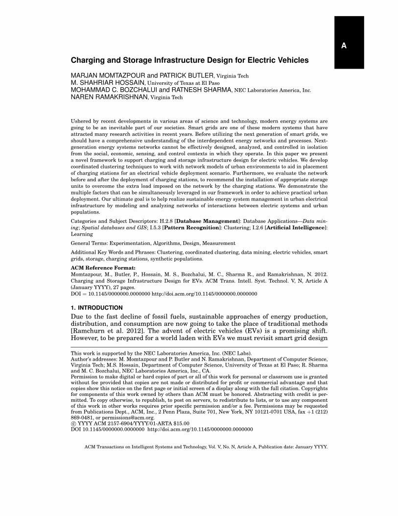
3. METHODOLOGYOur overall methodology is given in Figure 1. We describe each of the steps in ourapproach next. At a basic level, we integrate two basic types of data to formulate ourdata mining scenario. The first data, as described earlier, is a synthetic populationof people and activities representing the city of Portland and the second data set iselectricity consumption profile of each location. Notice that the proposed methodologyis a generic approach and can be applied to real-world data and the fact that we usesynthetic data here is only due to our lack of access to real-world data to test ourproposed methodology.

The synthetic dataset contains 243,423 locations of which 1,779 belong to the down-town area and of further interest for our purposes. Each location is represented bygeographical [x,y] coordinate adopting the universal transverse mercator coordinatesystem (UTM) [Bisset et al. 2006]. There are a total of 1,615,860 people in the en-tire city. Information about them is organized into households, and for each householdwe have the details of number of people in the household, and the ages, genders, andincomes of each household member. Each person has a unique ID.

We have some information about each person including age, gender, income, andhis/her house ID. The typical movement patterns of people in a 27 hour period (whichincludes a typical day) are also available. A total of 8,922,359 movements are provided.In addition to starting and ending locations for people’s movements, this dataset alsoprovides the purpose of the movement, categorized into nine types: {Home, Work, Shop,Visit, Social/Recreational, Serve Passenger, School, College, and Other}. A given per-son moves from one location to another location at a specific time for a specific purpose(from the nine mentioned above) and stays in that location for a specified period oftime. These movement types can thus be utilized for further detailed studies. We alsohave the ability to map the locations using Google Maps and calculate distances oftravel between locations.

To this dataset, we augment information about electricity consumption of each lo-cation and simulate the effects of EVs on its electricity demand profile. Since actualelectricity consumption data for each location is not available until all the consumershave smart meters installed and in operation for some time, we approximate electricityload profile using the existing data (organized by NEC Labs, America).

It is clear that the electricity load of each location greatly depends on the functional-ity of that location and hence our first approach is to utilize an information bottlenecktype approach [Tishby et al. 1999] to characterize locations. Our aim is to cluster loca-tions based on geographical proximity but such that the resulting clusters are highlyinformative of location function. This is thus our first application of a coordinated clus-tering formulation, and falls in the scope of clustering with side information. Next, weintegrate the electricity load information to characterize usage patterns across clusterswith a view toward helping identifying locations to place charging infrastructure.

Our next step is to more accurately characterize usage patterns of likely EV owners.A specific set of clusters from the previous pipeline is used and characterized usinghigh-income attributes as the likely owners of EVs. We then bring in additional fac-tors of locations that influence EV charger placement, e.g., residentiality ratio, loadon the location, charging needs, and typical duration of stay in the location. Some of



Information

bottleneck

Profiling 8 AM 9 AM -------

Feb 20, 11 0.16564 kW 0.23498 kW 0.3219 kW

Feb 21, 11 --- --- ---

---- --- --- ---

Synthetic population dataset

Electricity loads dataset

Characterizing

Locations

$70k $40k $100k $65k

© Google Maps, 2012

(a) Discovering location functionalities and characterizing electricity loads.

Coordinated

Clustering

Clusters of people

Clusters of locations

Clusters of

charging stations

EV owner characterization

Route travel

patterns Electricity load

patterns

© Google Maps, 2012

(b) Coordinated clustering of people, locations, and charging stations.

Charging Station

User Expectation

Storage

Placement

&

A

B

Charging Station Assignment

+

+

+© Google Maps, 2012

(c) Charging Station assignment and storage placement.Fig. 1. Overview of our methodology.

these factors (such as distance traveled) are in turn determined by mapping the home-to-work and work-to-home trajectories of EV owners and their stop locations. In theproposed method, three datasets are used. Two datasets describe locations and one of



them describes people. Since each location has a set of features which do not depend onits coordination, we use one dataset to describe specific features of each location andanother dataset that only consists of geographical coordinates. In addition to datasetsthat describe locations, we use a separate dataset for people with different income.

Choosing a right set of locations to install charging stations depends on many fea-tures. These features can be categorized into two groups: 1) Features of people whovisit those locations. It is better to assume that these people have EVs, and becausewe assume that people with higher income have EVs, it is preferable to choose loca-tions which people with higher incomes visit frequently. 2) Features of locations suchas electricity load. In fact, we are looking for a set of candidate locations that have sim-ilar features and also, are visited by same type of people. Among different data miningapproaches [Ramakrishnan and Grama 2001], clustering techniques can identify sim-ilarities and can categorize locations into different sets.

We use a coordinated clustering formulation to simultaneously cluster threedatasets in a relational setting. Coordinated clustering tries to cluster differentdatasets such that relationships between items in each dataset are preserved. Here,we try to identify best locations to install charging stations where certain groups ofpeople visit those locations. Candidate locations for charging stations are the onesthat have specific characteristics such as low electricity load. However, we try to findthose locations that have direct relationship with a specific group of people (peoplewith high income). Obviously, type of features in people dataset is different from loca-tions dataset. Due to this difference, and due to many-to-many relationship betweenlocations and people we cannot use regular clustering approaches such as k-means.Our coordinated clustering framework builds upon our previous work [Hossain et al.2010] which generalizes relational clustering between two non-homogeneous datasets.This problem is a bit non-trivial since one of the relations is a many-to-many relationand another is a one-to-one relation. The final set of coordinated clusters are then usedas interpretation and as a guide to charger placement.

After locating the homes of EV owners, we can determine their trajectories and theirstop locations. Then, based on this data, we can estimate their travel distances. Thishelps us estimate charging requirements of EVs, during a day. With the help of the dis-tribution of electricity load in the city and charging needs of EVs, we determine properlocations for installing charging stations in city with respect to specific parameters.

In addition, we come up with the actual scenario for each EV owner, who needscharging to see which locations are the best ones for him with respect to chargingcost and waiting time of EV owner. After measuring additional load of each chargingstation, we calculate the size of storage they need in order to reduce net load. Finally,we consider the economical aspects of storage deployment.

4. ALGORITHMSAs described in Section 3, our methodology comprises the following six major steps todetermine candidate locations for charging stations:

i discovering locations’ functionalities using an information bottleneck method;ii electricity load estimation and integration with results of previous step;

iii studying the behavior of EV owners and calculating specific parameters relevantto their usage patterns;

iv candidate selection for charging stations using coordinated clustering techniques;v finding appropriate charging stations for each user while maximizing user benefits;

andvi calculating the actual load of charging stations and storage placement.

Each of these steps are detailed next.



5.24 5.245 5.25 5.255 5.26

x 105

5.039

5.0395

5.04

5.0405

5.041

5.0415

5.042x 10

6 Clustering Results by Geography (60 clusters)

X

Y

5.24 5.245 5.25 5.255 5.26

x 105

5.039

5.0395

5.04

5.0405

5.041

5.0415

5.042x 10

6 Clustering Results by comparision among behavior of people

X

Y

Area 1Area 2Area 3Area 4

(a) (b)

0 5 10 15 20 250

0.5

1

1.5

2

2.5

3

3.5

4

4.5

5x 10

4

Time

Pop

ulat

ion

Population of 4 different areas over time

Area 1Area 2Area 3Area 4

5.24 5.245 5.25 5.255 5.26

x 105

5.039

5.0395

5.04

5.0405

5.041

5.0415

5.042x 10

6

X

Y

0.0469

0.0489

0.0666

0.2867

(c) (d)

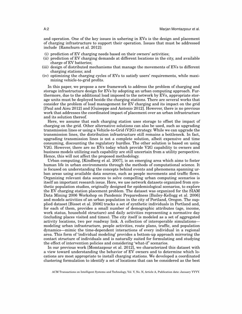
Fig. 2. (a) Clustering downtown locations based on geographic coordinates. (b) Clustering over the previousclustering with people’s activities as side-information. (c) Dynamic population of the four discovered clustersover a typical day. (d) Computed residentiality ratio revealing one primary residential cluster.

4.1. Discovering Location FunctionalitiesWe use information bottleneck methods to characterize locations with a view towarddefining the specific purpose of the location. The idea of information bottleneck meth-ods is to cluster data points in a space (here, geography) such that the resultingclusters are highly informative of another random variable (here, function). We fo-cus on 1779 locations in the downtown Portland area whose geographies are de-fined by (x,y) coordinates and whose functions are given by a 9-length profile vectorP = [p1, p2, ..., p9], where pi is the number of travels incident on that location for the ithpurpose (recall the different purposes introduced in the previous section).

Figure 2 (a) describes the results of a clustering based on Euclidean metrics be-tween locations whose results are aggregated in Figure 2 (b) into a revised clusteringthat also preserves information about activities of people at these locations. It is worthmentioning that in this part of our method, we desire to consider nearby locations andtheir electricity loads. Hence, the most appropriate approach for distance measure-ment is using Euclidean distance. The population distribution of these clusters overtime is shown in Figure 2 (c) which reveals characteristic changes of crowds aroundpeak hours and lunch times. One final analysis that will be useful is to evaluate eachof the discovered clusters with respect to what we term as the residentiality ratio. Theresidentiality ratio for a location is the percentage of people who use that location asa home w.r.t. all people who visit that location (in downtown Portland, many locations



0 5 10 15 20 250.2

0.3

0.4

0.5

0.6

0.7

0.8

0.9

1

1.1

1.2

Time

Ele

ctric

ity L

oad

Residential Area − each curve represents a day

Weekdays 1Summer and HolidaysWeekdays 2

0 5 10 15 20 250.5

1

1.5

2

2.5

3

3.5

4

4.5

5

Time

Ele

ctric

ity L

oad

Small office − each curve represents a day

Weekdays 1Weekdays 2Weekend

(a) (b)

0 5 10 15 20 250.5

1

1.5

2

2.5

3

3.5

4

Time

Ele

ctric

ity L

oad

Large office − each curve represents a day

Weekdays 1Weekdays 2Weekend

0 5 10 15 20 25

0.8

1

1.2

1.4

1.6

1.8

2

2.2

2.4

2.6

Time

Ele

ctric

ity L

oad

College − each curve represents a day

Holiday, breaks, SummerWeekdaysWeekends

(c) (d)

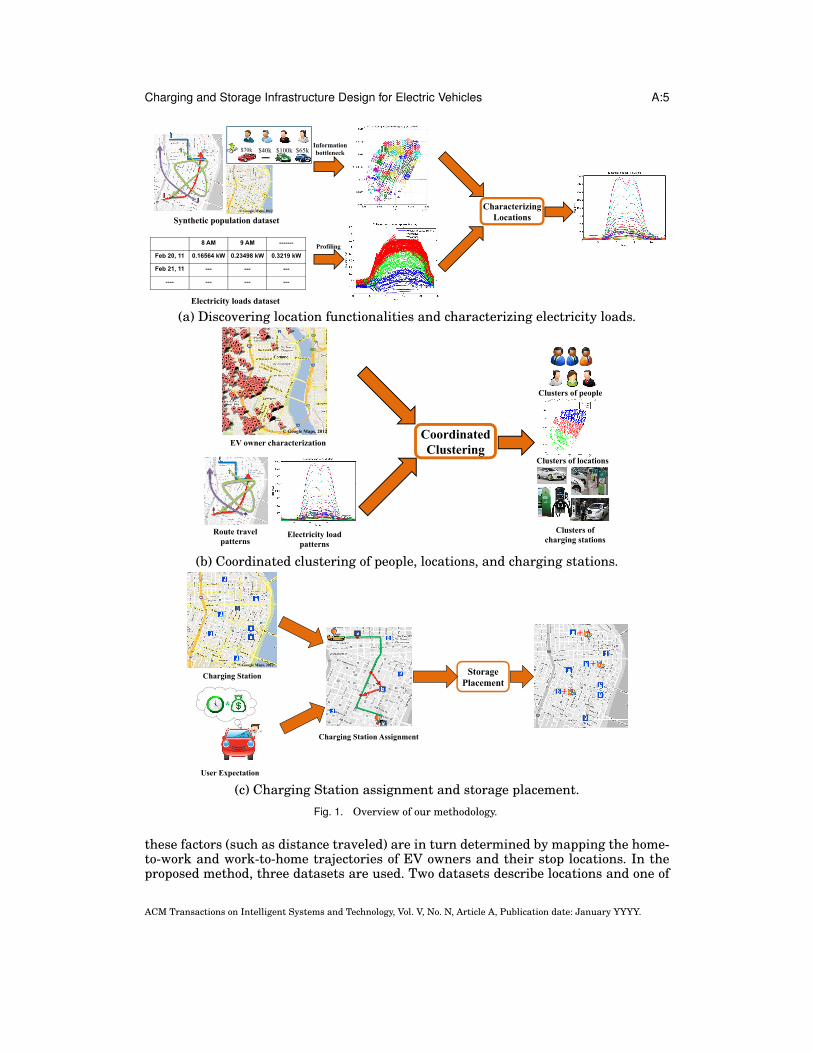
Fig. 3. (a) Electricity usage in residential areas. (b) Electricity usage in small office areas. (c) Electricityusage in large office areas. (d) Electricity usage in college areas.

have combined home-work profiles, and hence the calculation of residentiality ratiobecomes relevant). Figure 2 (d) reveals one cluster with relatively high residentialityratio among three others.

4.2. Electricity Load EstimationIn order to uncover patterns in electricity load distributions, we now characterize eachof the discovered clusters using typical profiles gathered from public data sources suchas the California End User Survey (CEUS) and other sources of usage information.Figure 3 presents daily electricity consumption profile across large offices, small of-fices, residential buildings, and colleges for one year. By clustering this data across theyear, we can discern important patterns associated with different types of consump-tion during the year. For instance, in the college setting, we can discern three types ofconsumption patterns: holiday breaks (including summer), weekdays, and weekends.

Our next step is to compute the electricity load leveraging the above patterns butw.r.t. our network model of the urban environment. Recall that our network model isbased on population dynamics but typical electricity load sources are based on squarefootage calculations. We map these factors using well-accepted measures, i.e., by con-sidering the average square footage occupied by one person in a residential area as600sft [Blake et al. 2007], small office as 200sft [U.S. General Services Administration1997], large office as 200sft [U.S. General Services Administration 1997], college as50sft [The Engineering ToolBox ], retail area as 50sft [The Engineering ToolBox ], and



Fig. 4. Electricity loads for four characterized location clusters.

other classes as 200. Further, the minimum population for an office to be consideredas a large office is set to 300.

Based on some exploratory data analysis, we selected a weekday in the past (specif-ically, 18th March, 2011) and used the electricity load data of this day to map to thenetwork model. Consider that in a specific hour, N people go to location l in which ni ofthem come for the purpose of pi while

∑9i=1 ni = N . Then the electricity load for that

location is computed as

El =

9∑i=1

niApiEpi1000

, (1)

where Api is the average square footage per person for the purpose Pi and Ep is elec-tricity consumption of building type p. It worth mentioning that Ep is from publicdata sources (California End User Survey (CEUS)) organized by NEC labs, Amer-ica. Observe that a single location can serve multiple purposes and the above equa-tion marginalizes across all uses. For example, if there are 360 people in one loca-tion, and 10 of them are in the building for the purpose of home and 350 are for thepurpose of office, the total electricity consumption of building would be calculated as(10 × 600 × Ephome/1000) + (350 × 200 × Epoffice/1000) where 600 and 200 are averagesquare footage per person for the different categories, as mentioned earlier. The abovemethodology enables us to characterize electricity loads in terms of the four locationclusters characterized in the previous step (see Figure 4).

4.3. Characterizing EV usersCurrently only a small percentage of people use EVs, and this figure is correlated withhigh income. Based on [Munro ] and [Simply Hired, Inc. ], only 6 percent of people inthe US have income more than 170,000 USD. In our synthetic dataset, 329,218 peoplemake an income greater than 60,000 USD. To explore a hypothetical scenario, we posedthe question:

What if 6.31% of 329,218 people from Portland bought EVs? What charginginfrastructure is necessary to support this scenario?

Based on [KEMA, Inc. 2012] this is a realistic assumption if we consider different pen-etration scenarios in U.S in forecasted EV adoption in 2012-2022. Based on our model-



ing of these people’s movements and patterns, we aim to identify the best locations forcharging stations.

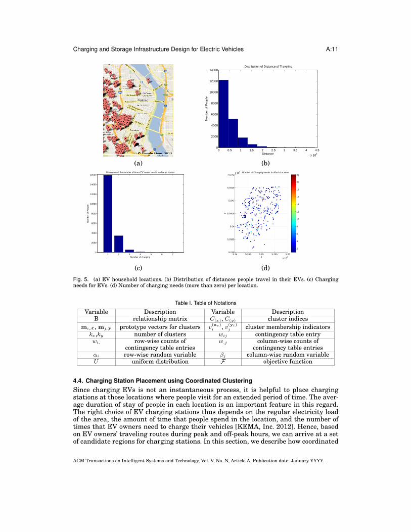
Figure 5 (a) gives the distribution of EV users in our potential scenario. We can no-tice several clusters around high-income neighborhoods. With the aid of Google Maps,we can estimate the amount of time an EV owner drives and how far he/she travels ona regular week day. Figure 5 (b) gives the distribution of distances traveled by theseusers.

Assuming EV owners charge their cars at their respective homes for beginning/endof day situations, our goal is now to identify candidate charging locations during othertimes. Candidate charging stations will be a critical issue in near future as the numberof EVs increases [Richard Martin 2012]. Let us assume that the EV of a person Pconsumes ECP KWh energy per 100 Km. Also, assume that the battery of this vehiclecan save ESP KWh. Then the estimated total distance that P can travel with his vehiclebefore he needs to charge its battery is

∆P =100ESPECP

, (2)

As an example, for the Chevrolet Volt [GM-Volt ], with ESP = 16 KWh and ECP = 22.4KWh per 100 Km, the EV can travel 71.43 Km before it needs to be recharged.

If the total traveling distance of P in a day is DP then the number of times that Pneeds to charge his vehicle is NP and is determined as follows:

NP =

⌊DP

∆P

⌋, (3)

As an example, if we assume that an EV’s battery can save 16 KWh energy [GM-Volt], an electric car can go for 71.43 Km before it needs to be charged [The official U.S.Government Source for Fuel Economy Information ].

Due to the long duration of charging process, we have a constraint to install chargingstations only in destinations that people visit. Assume that VL is the set of EV ownerswho visited location L during the day. Then |VL| is the total number of EV ownerswho have visited location L. However, there is a greater chance for a location to bea charging station if people with higher charge needs visit that location. Hence, thecharge needs of location L is determined based on equation 4.

WL =∑P∈VL

NP , (4)

Charging needs is an estimation to see in which locations, EV owners will probablycharge their EVs. It does not mean that vehicles will certainly charge at every location.Here, we say that “there is a greater chance for a location to be a charging station ifpeople with higher charge needs visit that location”. Equation (4) does not mean thatvehicles will charge at every visit to such locations. It is just a measure that indicateswhich locations have higher chance of experiencing charging needs. For example, iflocation A is visited by 10 EVs where all of them need to be charged only once duringa day, then charging need of location A would be 10. On the other hand, if location Bis visited by 8 EVs in which all of them need to be charged twice, then the chargingneed of location B would be 16, which is higher than A’s. These numbers show thatwith higher probability people in location B require charging needs, compared with A.

Figure 5 (c) depicts the histogram of how many times an EV needs to be charged.Also, Figure 5 (d) depicts the charge needs of downtown locations.



0 0.5 1 1.5 2 2.5 3 3.5 4 4.5

x 105

0

2000

4000

6000

8000

10000

12000

14000Distribution of Distance of Traveling

Distance

Num

ber

of P

eopl

e

(a) (b)

1 2 3 4 5 6 70

2000

4000

6000

8000

10000

12000

14000

16000

Num

ber

of P

eopl

e

Histogram of the number of times EV owner needs to charge his car

Number of charging5.24 5.245 5.25 5.255 5.26

x 105

5.039

5.0395

5.04

5.0405

5.041

5.0415

5.042x 10

6

X

Y

Number of Charging Needs for Each Location

2

4

6

8

10

12

14

16

18

20

22

(c) (d)

Fig. 5. (a) EV household locations. (b) Distribution of distances people travel in their EVs. (c) Chargingneeds for EVs. (d) Number of charging needs (more than zero) per location.

Table I. Table of Notations

Variable Description Variable DescriptionB relationship matrix C(x), C(y) cluster indices

mi,X , mj,Y prototype vectors for clusters v(xs)i , v(yt)

j cluster membership indicatorskx,ky number of clusters wij contingency table entrywi. row-wise counts of w.j column-wise counts of

contingency table entries contingency table entriesαi row-wise random variable βj column-wise random variableU uniform distribution F objective function

4.4. Charging Station Placement using Coordinated ClusteringSince charging EVs is not an instantaneous process, it is helpful to place chargingstations at those locations where people visit for an extended period of time. The aver-age duration of stay of people in each location is an important feature in this regard.The right choice of EV charging stations thus depends on the regular electricity loadof the area, the amount of time that people spend in the location, and the number oftimes that EV owners need to charge their vehicles [KEMA, Inc. 2012]. Hence, basedon EV owners’ traveling routes during peak and off-peak hours, we can arrive at a setof candidate regions for charging stations. In this section, we describe how coordinated



clustering can be used for charging station placement. Notations are summarized inTable I.

Let X be the income dataset and Y be the locations datasets. X = {xs}, s = 1, . . . , nxis the set of vectors in dataset X , where each vector is of dimension lx, i.e., xs ∈ Rlx .Currently, our income dataset contains only one dimension. Similarly, locations datasetY = {yt}, t = 1, . . . , ny,yt ∈ Rly . Locations are denoted by two dimensions (latitude andlongitude) in our current database. The many-to-many relationships between X andY are represented by a nx × ny binary matrix B, where B(s, t) = 1 if xs is relatedto yt, else B(s, t) = 0. Let C(x) and C(y) be the cluster indices, i.e., indicator randomvariables, corresponding to the income dataset X and location dataset Y and let kx andky be the corresponding number of clusters. Thus, C(x) takes values in {1, . . . , kx} andC(y) takes values in {1, . . . , ky}.

Let mi,X be the prototype vector for cluster i in income dataset X (similarly mj,Y

). These are the variables we wish to estimate/optimize for. Let v(xs)i (likewise v(yt)

j )be the cluster membership indicator variables, i.e., the probability that income datasample xs is assigned to cluster i in the income dataset X (resp). Thus,

∑kxi=1 v

(xs)i =∑ky

j=1 v(yt)j = 1. The traditional k-means hard assignment is given by:

v(xs)i =

{1 if ||xs −mi,X || ≤ ||xs −mi′,X ||, i′ = 1 . . . kx,0 otherwise.

(Likewise for v(yt)j .) Ideally, we would like a continuous function that tracks these hard

assignments to a high degree of accuracy. Such a continuous function for the the clustermembership can be defined as follows.

v(xs)i =

exp(− ρD ||xs −mi,X ||2)∑kx

i′=1 exp(− ρD ||xs −mi′,X ||2)

(5)

where ρ is a user-settable parameter and D is the pointset diameter which dependson the data. An analogous equation holds for v(yt)

j . Since our method operates overthe prototypes, and uses membership probabilities to compute the probability distri-bution of the contingency table, it is mandatory that the functions are smooth andcontinuous everywhere in the system. These are the essential properties of our objec-tive function. Any smooth and continuous membership function should work similarly.However, equation 5 has the advantage of involving Kreisselmeier-Steinhauser (KS)envelope function [Kreisselmeier and Steinhauser 1979] that is smooth and infinitelydifferentiable. As a result, our objective function can be optimized using any standardlocal and global optimizer.

We prepare a kx × ky contingency table to capture the relationships between entriesin clusters across income dataset X and locations dataset Y. To construct this contin-gency table, we simply iterate over every combination of data entities from X and Y,determine whether they have a relationship, and suitably increment the appropriateentry in the contingency table:

wij =

nx∑s=1

ny∑t=1

B(s, t)v(xs)i v

(yt)j . (6)

We also define

wi. =

ky∑j=1

wij , w.j =

kx∑i=1

wij ,



where wi. and w.j are the row-wise (income cluster-wise) and column-wise (locationscluster-wise) counts of the cells of the contingency table respectively.

We also define the row-wise random variables αi, i = 1, . . . , kx and column-wise ran-dom variables βj , j = 1, . . . , ky with probability distributions as follows

p(αi = j) = p(C(y) = j|C(x) = i) =wijwi.

. (7)

p(βj = i) = p(C(x) = i|C(y) = j) =wijw.j

. (8)

The row-wise distributions represent the conditional distributions of the clusters indataset in X given the clusters in Y; the column-wise distributions are also interpretedanalogously.

After we construct the contingency table, we must evaluate it to see if it reflectsa coordinated clustering. In coordinated clustering, we expect that the contingencytable will be nonuniform. We can expect that the contingency table will be an identitymatrix when kx = ky. To keep the formulation and the implementation generic fordifferent number of clusters in two dataset, we need to optimize the variables (clusterprototypes) in such a way that the contingency table is far from its uniform case. Forthis purpose, we compare the income cluster (row-wise) and locations cluster (column-wise) distributions from the contingency table entries to the uniform distribution.

We use KL-divergences to define our unified objective function:

F =1

kx

kx∑i=1

DKL

(αi||U

(1

ky

))+

1

ky

ky∑j=1

DKL

(βj ||U

(1

kx

)), (9)

where DKL is the KL-divergence between two distributions and U indicates the uni-form distribution over a row or a column. The idea of KL divergence is to estimate dis-crimination of information (Minimum Discrimination Information (MDI)) that leadsus to use it as our divergence measure. Similar techniques that follow the MDI princi-ple have the potential to be a part of our objective function. In the future, we plan toperform extensive experiments on this.

Note that the row-wise distributions take values over the columns 1, . . . , ky and thecolumn-wise distributions take values over the rows 1, . . . , kx. Hence the reference dis-tribution for row-wise variables is over the columns, and vice versa. Also, observe thatthe row-wise and column-wise KL-divergences are averaged to form F . This is to miti-gate the effect of lopsided contingency tables (kx � ky or ky � kx) wherein it is possibleto optimize F by focusing on the “longer” dimension without really ensuring that theother dimension’s projections are close to uniform.

Maximizing F leads to rows (income clusters) and columns (locations clusters) inthe contingency table that are far from the uniform distribution as required by thecoordinated clusters. It is equivalent to minimizing −F .

The coordinated clustering formulation presented thus far can have some degener-ate solutions where large number of data points in both datasets are assigned to thesame cluster leading to a huge overlap of relationships. To mitigate this, we add twomore terms with the objective function.

FR = −F +DKL

(p (α) ||U

(1

kx

))+DKL

(p (β) ||U

(1

ky

)). (10)



where p(α) and p(β) are defined as follows.

p (α) =1

nx

nx∑s=1

V (xs) (11)

p (β) =1

ny

ny∑t=1

V (yt). (12)

It should be noted that function FR is expected to be minimized. This is the reasonwhy −F is used in the formula for FR.

Finally, we describe how to integrate three datasets: income, location, and stationproperties. Let X , Y, and Z be these three datasets, respectively. There are two sets ofrelationships, existing between X , Y, and Y, Z. The objective function for these threedatasets and two sets of relationships is defined as follows.

FXYZ = FR (X ,Y) + FR (Y,Z) . (13)

Here FR (X ,Y) refers to the objective function described in Eq. 10 with the incomedataset X , and locations dataset Y. FR (Y,Z) refers to the same objective functionbut input datasets are locations Y, and station property Z. In all our experiments, weminimize FXYZ to apply coordinated clustering between income, locations, and stationproperty datasets.

4.5. Charging Station Assignment based on User ExpectationsAfter determining candidate charging stations, we need to assess the effect of in-stalling charging stations at those locations, and evaluate the changes in electricityload. In addition, from a business point of view, it is important to study the size ofstorage needed at those locations.

First, we need to evaluate candidate charging stations resulting from our co-clustering algorithm. One solution is to see whether these set of candidates are evenused by EV owners. In order to understand which locations tend to be charging sta-tions from EV owners’s point of view, we need to identify the desired locations of eachperson. These locations are the ones that minimize cost of charging for EV owners. Onthe other hand, since the process of charging an EV typically will take several hours,user tends to charge his car in those locations where he stays for at least a few hours.Obviously, from a business point of view, we not only consider those locations thatmeet users’ criteria (charging cost), but also aim to optimize charging station in termsof electricity load and size of storage.

In this subsection, we show how to determine where users desire to charge theirvehicles with respect to cost of charging and change of route for each user. In whatfollows, we develop an algorithm to assign charging stations to users. Of course, usershave the freedom to select their charging stations. We assume that they are intuitivelylooking for the cheapest options. Also, we assume that users desire to minimize theirdetour and their waiting time (for charging). These assumptions were considered inthe assignment algorithm. This assignment requires an estimate of storage sizes ofcharging stations. For this reason, we need to know the exact schedule of users tocalculate the overall electricity load of each location. We assume that detour, cost, andwaiting time are important issues in selecting charging stations for all users. (It shouldbe noted that the goal here is to estimate the storage size, not to suggest chargingstations to users.)



ALGORITHM 1: User-based Candidate Charging Stations (UCCS)Input: Route consists of sequence of locations.Output: ChargingStations consists of best locations to charge as well as level of charging and

time of charging at those locations.CS= RUCCS(Route(1), R,Route) /* assume at first each car has fully charged (R) */MinFailure = min(CS(Failure));MinFailureSet =subset of CS with Failure equal to MinFailure;ChargingStations = argmin(MinFailureSet(Cost));return ChargingStations

To the best of our knowledge, there is limited work on the “where to charge” problemin the literature. In [Khuller et al. 2011], authors try to find the cheapest tour betweencustomer destination locations to fill gas. Our work is different from [Khuller et al.2011] for a variety of reasons. For example, in our problem,

(1) Sequence of stop points for each user is determined.(2) We do not have a boundary on the number of times that an EV owner can charge

his car.(3) Price of charging in each location varies based on duration of stay of user in that

location.(4) In some locations, car battery will be charged partially.

Before explaining our algorithm, it is worth mentioning that there are different stan-dards for charging stations. Charging time of each EV depends on its capacity and thecharging level of the charger. Levels of charging for EVs can be categorized into threelevels: level 1, level 2, and level 3 (DC power). Power consumption of each level is dif-ferent from each other and hence, prices are different. Furthermore, rate of charging(the time that it takes to charge a battery for 1 KWh) is different for each level.

The algorithm for estimating desired charging locations based on user point of viewis as follows:

For each user, we invoke Algorithm 1 (UCCS). This algorithm takes the route of oneuser as input and calculates the best locations for charging as well as level of chargingand the time of charging. Algorithm 1 calls Algorithm 2 to compute all feasible sets ofcharging stations in the route that user travels. Then, Algorithm 1 only retains thosesets that have minimum number of failures, i.e. minimum number of times that carhas to switch to gas because of empty battery. After that, it selects a set of chargingstations which has a minimum cost of charging.

Algorithm 2 (RUCCS) is a recursive function for finding all feasible sets of chargingstations. It takes the current location, remaining charge in the EV, and the route ofuser as inputs and calculates sets of candidate charging stations. This algorithm worksas follows:

Let us assume that currently the EV is at location Lj , and that the available chargeof battery is equal to Cj . Also, assume that d, the distance that the EV can travelfrom Lj without charging its battery, can be computed. This distance is determined inLine 2. Here, R is the capacity of the battery and D is the distance that EV can travelwith a fully charged battery. In Line 3 of the algorithm, we determine A as the set oflocations that are located on the route of EV, and are at most d meters away from Lj .It is obvious that if the last point of the route is in A, we do not need to re-charge thebattery (Lines 4-6). On the other hand, the EV must re-charge its battery in at leastone of the locations in A; otherwise after d meters, it should switch to gas.

However, when A is empty, there is no way to re-charge the battery of EV. In thatcase, EV must switch to gas and we say that a failure has happened. After a failure,



in the next subsequent stop point, Lj+1, EV’s battery must be re-charged. In this case,we recursively call RUCCS for Lj+1 (Lines 8-23). Here, MaxCj+1,k is the maximumpossible charge of battery which is determined based on duration of stay of the car,and level of charge, k. However, because the capacity of battery is R, the actual valueof the charge is calculated in line 11 and is shown by Cj+1,k. Cost of this charge isdetermined in line 12 by CostCj+1,k.

If A is not empty (line 24), we must choose the most feasible location in A for re-charging the battery. Therefore, in Lines 25-32, for each location in A, and for eachcharging level, k, we calculate the amount of possible charge in that location (Ci,k),the cost of charging (CostCi,k), and the maximum distance that the car will travel(MaxDi,k), if we charge it in that location with that charging level. For each charginglevel, the best stop point for re-charging the car is the one that if we re-charge ourvehicle there, we can travel further with respect to the current location, Lj .

Choosing the best members of A for re-charging is performed in Line 33. Then, ifthe best stop point for charging level k is Lidx, we recursively call RUCCS with inputsLidx, Cidx,k, and Route (Line 34). After returning from a recursive call of RUCCS fora location such as Li, (Lines 13 and 34), we have several sets of stop points that areconsidered as feasible sets located after Li. These sets are determined with this as-sumption that Li is a charging station too. Hence, we have to add Li to all of these setsbefore returning from the current iteration of the algorithm (Lines 14-19 and 35-40).Also, because we want to consider all feasible solutions to choose the best one, we haveto keep all the results that are determined for different charging levels. This step isperformed in Lines 20 and 41.

After determining the most feasible locations from the users perspective, i.e. loca-tions that minimize charging cost and number of failure’s, we must match existingcharging stations with the new locations. Since, we cannot establish charging stationfor each location that users want, we choose those charging stations that were ex-tracted from Section 4.4 and assign each user to them based on distance to chargingstations. Hence, for each charging station, we know when and how many times it willserve EVs. In order to select the best charging stations for a user, we use a nearestcharging station assignment policy. Therefore, if the desired location for charging is Liand Sc is the set of available charging stations we use Ci instead of Li where

Ci = argmin distance(Li, Cj) for all Cj in Sc (14)

where, distance(A,B) measures the distance between locations A and B. It should bementioned that any method of distance measurement (Euclidean, Manhattan, ...) canbe used in this function.

With this policy, detours are minimized. After assigning charging stations, theamount of electricity load added to charging stations based on their serving time willbe calculated.



ALGORITHM 2: Recursive Function (RUCCS)Input: Lj is the current location, and Cj is available charge of car at location Lj and Route

consists of sequence of locations.Output: CS which consists of sets of candidate charging stations. Each candidate charging set

(CSi) has the following fields:CSi(points) is the ordered set of locations where user must charge his car.CSi(level) is level of charging at each location in CSi(points).CSi(costs) is cost of charging at each location.CSi(Failure) is the number of failure during trip.

1 CS = {};2 d = Cj ∗ D

R

3 A = set of stop points in distance d of Lj ;4 if Route(end) is in A then5 return CS;6 end7 if |A| = 0 then /* failure will happen and it must switch to gas */8 Lj+1 = next subsequent stop point in Route;9 for k = 1 to 3 do

10 MaxCj+1,k =maximum possible charge at Lj+1 with level k;11 Cj+1,k = min(MaxCj+1,k, R);12 CostCj+1,k =cost of charging at Lj+1 with level k;13 CSk = RUCCS(Lj+1, Cj+1,k, Route);14 for each candidate set, CSk

m, in CSk do15 CSk

m(points) = [Lj+1 CSkm(points)];

16 CSkm(levels) = [k CSk

m(levels)];17 CSk

m(costs) = [CostCj+1,k CSkm(costs)];

18 CSkm(failure) = CSk

m(failure) + 1;19 end20 CS=CS ∪ CSk;21 end22 return CS;23 else24 for each point, Li, in A do25 for k = 1 to 3 do26 MaxCi,k =maximum possible charge at Li with level k;27 Ci,k = min(Cj − dist(Lj ,Li)∗R

D+MaxCi,k, R);

28 CostCi,k =cost of charging at Li with level k;29 MaxDi,k = D

R∗ Ci,k + dist(Lj , Li);

30 end31 end32 for k = 1 to 3 do33 idx = argmaxLi∈A(MaxDi,k);34 CSk = RUCCS(Lidx,k, Cidx,k, Route);35 for each candidate set, CSk

m, in CSk do36 CSk

m(points) = [Lidx,k CSkm(points)];

37 CSkm(levels) = [k CSk

m(levels)];38 CSk

m(costs) = [CostCidx,k CSkm(costs)];

39 CSkm(failure) = CSk

m(failure) + 1;40 end41 CS=CS ∪ CSk;42 end43 return CS;44 end



4.6. Storage PlacementIn previous section, we determined profile of electricity load at each location before andafter charging station deployment. Profile of electricity load after installing chargingstations is determined based on number of cars that are charged at each location andtheir corresponding level and duration of charging. On the other hand, each locationhas a predetermined capacity which is the maximum electricity load that it can toler-ate. When electricity load of a location increases and goes above its capacity, we needto place storage to meet the electricity demand of that location. In this regard, theefficiency of storage is also important. Here, we assume that the desired utilization ofstorage in all locations is 80% i.e. at most 80% of the capacity of a storage is used ina day. That ensures us that storage will not discharged to no more than 80% of totalcapacity. Due to the small size of storage at some locations we aggregate storages ofnearby locations. For this purpose, we use DBSCAN [Ester et al. 1996] to locate denseareas and calculate the needed storage size of each cluster as a summation of storagesover all locations in that cluster.

From a business point of view, placing storage at a charging station must have aadequate revenue for storage owners. In addition, putting storage at locations is ad-vantageous to city in terms of reducing the peak of electricity load in urban area.

To investigate the revenue of storage units, we consider each charging station in turnand compute the revenue of storage. Here, revenue refer to the amount of funds thatstorage owners will save from selling energy to consumers. Revenue can be achievedby selling energy during the day and recharging the storage during the night (withoff-peak rate). In addition, to observe profile of charging stations based on their loadcurves, we use the clustering algorithm introduced in [Yang and Leskovec 2011], i.e.,the K-Spectral Centroid (K-SC) algorithm for time series data using a similarity met-ric invariant to scaling and shifting. They apply adaptive wavelet-based incrementalapproach to K-SC to use it for large datasets. K-SC proved to be an effective clusteringwhen scaling is not important. By applying this method, we can understand differ-ent types of charging stations based on their load curves and finally, locate the bestlocations to put storage in order to get high revenue.

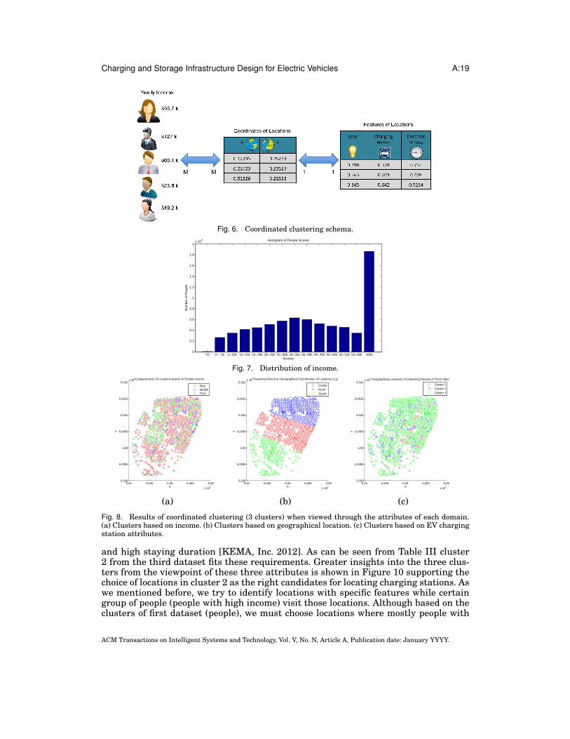
5. RESULTSFigure 6 describes the coordinated clustering scenario. As illustrated in this figure, weuse three datasets: People (Income), coordinates (x,y) of location, and features (load,charge need, stay) of location. First dataset contains information about income of peo-ple and second dataset has information about the geographic coordinates of each loca-tion. However, the third dataset contains the characteristics of locations for chargingstation placement. Electricity load of buildings, charging need of people in that locationand duration of stay in each location are three features in this dataset.

We begin with some preliminary observations about our data. Figure 7 depicts thedistribution of people based on their income, indicating that a significant number ofpeople have high income, leading to a large number of EV users. We experimentedwith coordinated clustering settings involving many settings. Figure 8 depicts threeclusters of locations based on each of the attribute sets in our schema. Note that be-cause the clusters are mapped onto (x,y) geographical locations, locality is apparentonly in Figure 8 (b).

Profiles of these clusters are described in detail in Figure 9. Of particular interestto us is the view from the perspective of EV attributes, i.e., Figure 9 (c). Details ofthese clusters are explored in greater detail in Table III. Ideal locations for chargingstations for EVs must have a relatively low current electricity load (to accommodatethe installation of charging infrastructure), high charging needs (population profiles),



Fig. 6. Coordinated clustering schema.

<0 0 − 5k 5−10k 10−15k 15−20k 20−25k 25−30k 30−35k 35−40k 40−45k 45−50k 50−55k 55−60k >60k0

0.2

0.4

0.6

0.8

1

1.2

1.4

1.6

1.8

2x 10

4

Num

ber

of P

eopl

e

Income

Histogram of People Income

Fig. 7. Distribution of income.

5.24 5.245 5.25 5.255 5.26

x 105

5.039

5.0395

5.04

5.0405

5.041

5.0415

5.042x 10

6

X

Y

Categorization of Locations based on People Income

RichMiddlePoor

5.24 5.245 5.25 5.255 5.26

x 105

5.039

5.0395

5.04

5.0405

5.041

5.0415

5.042x 10

6

X

Y

Clustering Result on Geographical Coordination of Locations (x,y)

CenterNorthSouth

5.24 5.245 5.25 5.255 5.26

x 105

5.039

5.0395

5.04

5.0405

5.041

5.0415

5.042x 10

6

X

Y

Geographical Locations of Clustering Results of Third Table

Cluster 1Cluster 2Cluster 3

(a) (b) (c)

Fig. 8. Results of coordinated clustering (3 clusters) when viewed through the attributes of each domain.(a) Clusters based on income. (b) Clusters based on geographical location. (c) Clusters based on EV chargingstation attributes.

and high staying duration [KEMA, Inc. 2012]. As can be seen from Table III cluster2 from the third dataset fits these requirements. Greater insights into the three clus-ters from the viewpoint of these three attributes is shown in Figure 10 supporting thechoice of locations in cluster 2 as the right candidates for locating charging stations. Aswe mentioned before, we try to identify locations with specific features while certaingroup of people (people with high income) visit those locations. Although based on theclusters of first dataset (people), we must choose locations where mostly people with



Rich Middle Poor0

0.5

1

1.5

2

2.5

3

3.5x 10

4

Num

ber

of P

eopl

e

Category of People

Population of Different Category of People based on Income

Center North South0

100

200

300

400

500

600

Cou

nt

Types of Clusters

Population of Different Types of Clusters in Second Table

Cluster 1 Cluster 2 Cluster 30

200

400

600

800

1000

1200

Num

bmer

of L

ocat

ion

Clusters

Distribution of Different Types of Clusters in Third Table (Features of Locations)

(a) (b) (c)

Fig. 9. Profiles of clusters obtained from coordinated clustering w.r.t. each of the three domains. (a) Incomeattributes. (b) Location attributes. (c) EV charging station attributions.


0.1

0.2

0.3

0.4

0.5

0.6

0.7

0.8

0.9

1

Types of Clusters

Variation of Electricity Load in Clusters of Third Table

MinMedianMeanMax


0.1

0.2

0.3

0.4

0.5

0.6

0.7

0.8

0.9

1

Types of Clusters

Variation of Charging Needs in Clusters of Third Table

MinMedianMeanMax

Cluster 1 Cluster 2 Cluste 30

0.1

0.2

0.3

0.4

0.5

0.6

0.7

0.8

0.9

1

Types of Clusters

Variation of Duration of Stay in Clusters of Third Table

MinMedianMeanMax

(a) (b) (c)

Fig. 10. Detailed inspection of clusters for their suitability for locating EV charging stations. (a) Distri-bution of electricity loads. (b) Distribution of charging needs. (c) Distribution of duration of stay. An idealcluster should have (low, high, high) values respectively, suggesting that cluster 2 is best suited.

Table II. Profiles of Clusters in Third Dataset (Location’s Features)

Cluster % of People with % of Locations with % of Locations with % of Locations withHigh income High Elec. load High Charging need High Stay

1 0.43 0.45 0 0.022 0.41 0.06 0.15 0.883 0.41 0.05 0.01 0.01

greater salary affordances visit, the distribution of high income vs. low income peoplein clusters 1, 2 and 3 in third dataset (locations) are almost similar. This is illustratedin Table II. With respect to distribution of high income people people, cluster 1 is bet-ter selected. However, cluster one is not a good choice for installing charging stationsbecause 45% of its locations are those with high electricity load. Between other twoclusters (cluster 2 and cluster 3), cluster 2 is better because it has low electricity load,high charging need, and high duration of stay.

With the aid of clustering, we can predict which locations are the best candidatesto install charging stations. However, the effect of installing charging stations in theselocations on other metrics such as the price of charging and electricity load of buildingsmust be evaluated.

Since we are looking only at downtown area of Portland, we do not have any in-formation about exact location of other charging stations outside of downtown. Here,we padded our downtown area by 500 meters from each side (if we suppose down-town has a rectangular shape). Then, assuming that those cars in the padded area canbe served by our current charging stations, we run the algorithm 1 for each car. Thedistance between charging station and current location of car must be minimized be-cause charging at charging station with Level 1 or 2 will take several hours and peopleprefer to charge their cars at those locations that they stay longer. In reality, users



Table III. Characteristics of Clusters in Third Dataset (Location’sFeatures)

Cluster Elec. Load Charging Need Stay Duration1 High Low Low2 Low High High3 Low Low Low

Table IV. Characteristics of Charging Stations

Level Description Elec. Load(kW) Cost(c//kWh) Time(h)on-peak mid-peak off-peak

1 110v outlet,16 Amp 2.2 16.62 10.85 7.77 82 220v charger, 16 Amp 3.3 16.62 10.85 7.77 43 400v DC, 125 Amp 50 10.89 6.36 3.63 0.5

can charge their cars anywhere in vicinity (∼1 mile) of their desired buildings (ex. hecan park his car at nearest charging station and walk to his office). Furthermore, weneed to have information for two types of movements (riding to charging station, andwalking to office). Since, the distances are not too large, using Euclidean distance tomeasure distances is not troublesome and makes computations easier. Furthermore,the actual information about roads of the area was not available to use and the datasetconsists only origin and destination of each movement.

Specifications of three levels of charging for Portland are summarized in Table IVbased on PGE [Portland General Electric Company 2012a] and [Portland General Elec-tric Company 2012b]. From [Portland General Electric Company 2012b], Schedule 7 ischosen for level 1 and 2 and Schedule 32 is selected for level 3. It is worth mention-ing that prices (tariff rate) are based on time of use policy (TOU). The definition ofOn-peak, Mid-peak, and Off-peak is inspired from the electricity loads in our dataset:

— On-peak: 6 AM to 10 AM and 5 PM to 8 PM— Mid-peak: 10 AM to 5 PM and 8 PM to 10 PM— Off-peak: 10 PM to 6 AM

Prices at Table IV are for both buying electricity from the grid and from chargingstation (by EVs). The type of charging depends on time of stay. If an EV stays for 8hours, it can charge by charging level 1 which is cheapest option. If an EV stays for 4hours, it can use level 2 charger whereas if the EV needs to be charged in 30 minutes,it can use the level 3 (DC) option. Price of charging in level 3 is very high compared tolevel one and two. For example, cost difference (a complete charging) between chargingby DC and level I would be 50∗10.89−2.2∗16.62 = 507.936 cents or $5. Hence, the overallimpact of level of charging (I, II, and DC) is very high on charging stations and on usersin cost and electricity load points of view.

Experiments show that average distance traveled by each car is 8.4881 meters andthat the maximum distance traveled in this experiment was 1188.2 meters. Figure 11(a) depicts the histogram of distance between location of current stop point and avail-able charging station. This result is promising since we considered part of the bound-aries of downtown while there might be a charging station in that area. The number ofcharging stations based on our clustering algorithm is 161 while number of locationsthat people liked to charge their cars is 367. The histogram of expenses that all EVowners in Portland will pay daily for charging is shown in Figure 11 (b).

Also, number of cars that are served at each charging station is important from abusiness point of view, to study revenue of charging station owners. As Figure 12 (a)shows this is zero for some charging stations (black circles) and they can be removedfrom consideration as charging station candidates. Based on this figure, we can place



0 200 400 600 800 1000 12000

100

200

300

400

500

600

Travel distance to reach Charging Station (meter)

Num

ber

of E

Vs

Histogram of Traveling Distance for EVs

0 100 200 300 400 500 600 7000

500

1000

1500

2000

2500Histogram of Money that people spend on Charging

Price ($)

Num

ber

of p

eopl

e

(a) (b)

Fig. 11. (a) Histogram of distance between current stop point of location and available charging station(meter). (b) Histogram of expenses people spend on charging during a day.

5.24 5.245 5.25 5.255 5.26

x 105

5.039

5.0395

5.04

5.0405

5.041

5.0415

5.042x 10

6

X

Y

Number of cars in Charging Station

2

4

6

8

10

12

14

16

18

20

22

24

5.24 5.245 5.25 5.255 5.26

x 105

5.039

5.0395

5.04

5.0405

5.041

5.0415

5.042x 10

6 Size of storages in charging stations of downtown (kWh)

X

Y

100

200

300

400

500

600

700

(a) (b)

Fig. 12. (a) Number of cars that served by each charging station. Note that some charging station (black cir-cle) are useless and can be removed. (b) Size of storage in charging stations (kWh). Note that some chargingstation (black circle) are useless and can be removed.

appropriate charging infrastructure at those locations that serve certain number ofcars.

It should be noted that the number of failures in our algorithm is 48. This highlightsthe number of cases where an EV must switch to gas in order to continue its route.Experiments show that all of these 48 cases was due to the nature of our dataset, i.e.distance between locations was more than maximum possible distance of travel with afull battery.

Those charging stations that provide service to cars will add extra load to the loca-tion. This load might be more than the capacity of the location. Here, we assume thatmaximum load of one location during a day is equal to its capacity. We must place stor-age to those locations that require extra electricity. For determining the size of storageat each charging station, we must look at values of location’s capacity and electricityload after adding EV. To compute size of storages, we would like to assume that stor-



0 0.1 0.2 0.3 0.4 0.5 0.6 0.7 0.80

5

10

15

20

25

30

35

40Histogram of time−based utilization

Time−based UtilizationN

umbe

r of

Sto

rage

Fig. 13. Histogram of Time-based Utilization.

5.24 5.242 5.244 5.246 5.248 5.25 5.252 5.254 5.256 5.258

x 105

5.0395

5.04

5.0405

5.041

5.0415x 10

6

51

267 186

446

421239

483

320

382

987

468

666

140

652247

812

111

252

261

137

163

229

100

167

63

108

75

4

170

29 region with their storage size (kWh)

X

Y

Fig. 14. Aggregated regions. Value of storage size (per kWh) is shown for each region (sum of all storages)

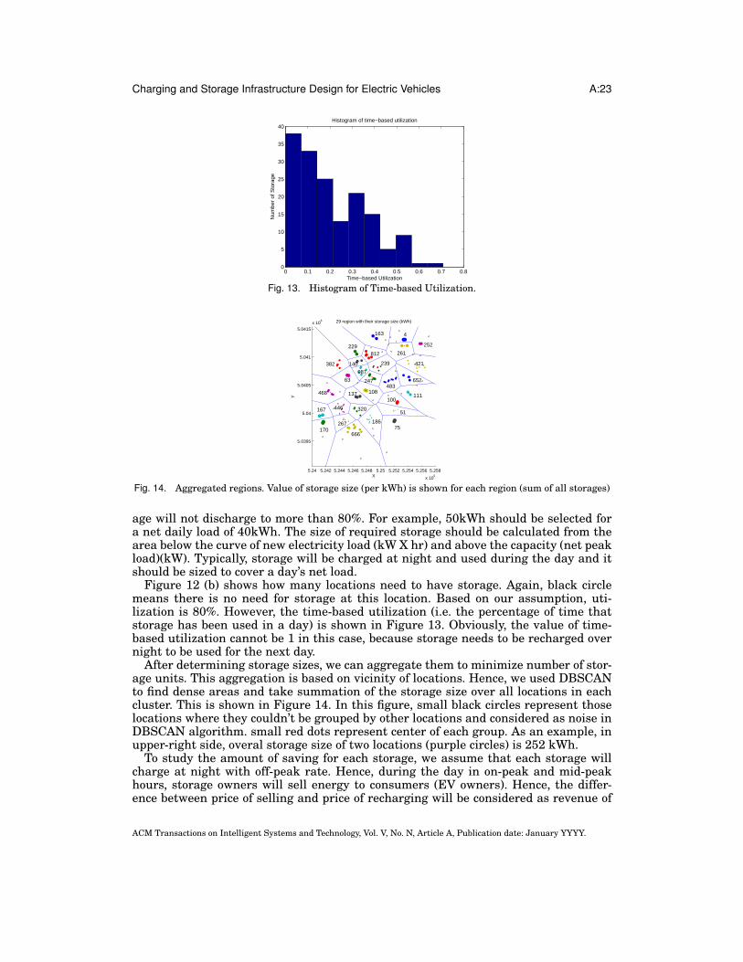
age will not discharge to more than 80%. For example, 50kWh should be selected fora net daily load of 40kWh. The size of required storage should be calculated from thearea below the curve of new electricity load (kW X hr) and above the capacity (net peakload)(kW). Typically, storage will be charged at night and used during the day and itshould be sized to cover a day’s net load.

Figure 12 (b) shows how many locations need to have storage. Again, black circlemeans there is no need for storage at this location. Based on our assumption, uti-lization is 80%. However, the time-based utilization (i.e. the percentage of time thatstorage has been used in a day) is shown in Figure 13. Obviously, the value of time-based utilization cannot be 1 in this case, because storage needs to be recharged overnight to be used for the next day.

After determining storage sizes, we can aggregate them to minimize number of stor-age units. This aggregation is based on vicinity of locations. Hence, we used DBSCANto find dense areas and take summation of the storage size over all locations in eachcluster. This is shown in Figure 14. In this figure, small black circles represent thoselocations where they couldn’t be grouped by other locations and considered as noise inDBSCAN algorithm. small red dots represent center of each group. As an example, inupper-right side, overal storage size of two locations (purple circles) is 252 kWh.

To study the amount of saving for each storage, we assume that each storage willcharge at night with off-peak rate. Hence, during the day in on-peak and mid-peakhours, storage owners will sell energy to consumers (EV owners). Hence, the differ-ence between price of selling and price of recharging will be considered as revenue of



5.24 5.245 5.25 5.255 5.26

x 105

5.039

5.0395

5.04

5.0405

5.041

5.0415

5.042x 10

6Daily energy storage revenue at charging stations (cents)

X

Y

200

400

600

800

1000

1200

1400

1600

1800

2000

2200

Fig. 15. Revenue of energy storage at charging stations

storage. Figure 15 shows energy storage revenue for each charging station that hasstorage unit. This value of revenue is calculated for one typical day.

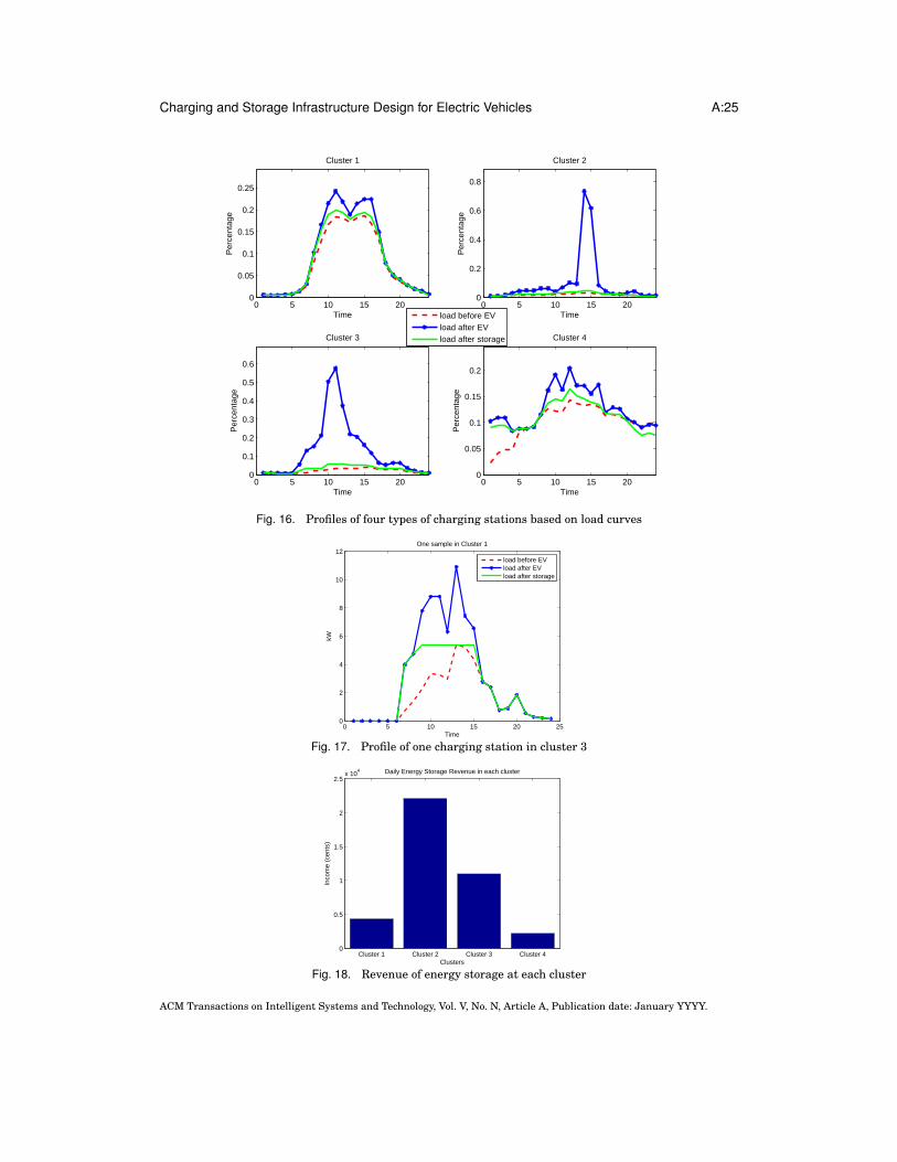
To observe the profiles of charging stations based on their load curves after addingEVs and after adding storage, we used the K-SC clustering approach described earlier.Here, the value of electricity load before adding EV, after adding EV, and after storagedeployment during 24 hours were considered as a vector of 24*3 elements. The profilesof charging stations are categorized into 4 clusters which the prototype of each clus-ter is shown in Figure 16. It should be noted that this clustering is invariant to shiftand scale and that is why the value of load after storage deployment is higher thanmaximum value of load before considering EV. Figure 17 depicts an example of actualcurves for one charging station in cluster 1. It is obvious that storage deployment willensure that the value of electricity load will not go higher than the capacity at each lo-cation. Figure 16 is important in understanding the behavior of charging stations. Alsothis figure is helpful in deciding between using a mobile storage unit and a stationaryone.

In Figure 16, charging stations in clusters 1 and 4 have little impact on the peakload, whereas those in cluster 2 and 3 significantly increase peak demand of the sys-tem. Therefore, using energy storage for charging stations in cluster 2 and 3 wouldmake more sense than in clusters 1 and 4. Based on number of charging stations ineach cluster, 43% of charging stations (in cluster 2 and 3) are candidates for storagedeployment. On the other hand, if there is no possibility of adding energy storage,charging stations in clusters 1 and 4 would have much less impact on the grid and willbe accepted by utilities with less opposition. Also, one can deploy mobile storage unitsfor charging stations in clusters 1 and 4.

Figure 18 shows the amount of daily revenue achieved by storage deployment foreach cluster. In this figure, locations in cluster 2 and 3 have highest revenue comparedwith cluster 1 and 4. Total revenue in cluster 1 and 4 is 6547.2 cents while total rev-enue in cluster 2 and 3 is 33081.0 cents. Based on this, one can justify using stationarybattery storage in candidate charging stations (cluster 2 and 3).

6. DISCUSSIONElectrical vehicles are going to become more popular in the near future. We havedemonstrated a systematic data mining methodology that can be used to identify loca-tions for placing charging infrastructure as well as storage infrastructure as EV needsgrow. In addition, we identified candidate locations for deployment of stationary en-ergy storages to utilize existing electricity infrastructure. The results presented herecan be generalized to a temporal scenario where we accommodate a growing EV pop-



0 5 10 15 200

0.05

0.1

0.15

0.2

0.25

Cluster 1

Time

Per

cent

age

0 5 10 15 200

0.2

0.4

0.6

0.8

Cluster 2

Time

Per

cent

age

0 5 10 15 200

0.1

0.2

0.3

0.4

0.5

0.6

Cluster 3

Time

Per

cent

age

0 5 10 15 200

0.05

0.1

0.15

0.2

Cluster 4

Time

Per

cent

age

load before EVload after EVload after storage

Fig. 16. Profiles of four types of charging stations based on load curves

0 5 10 15 20 250

2

4

6

8

10

12One sample in Cluster 1

Time

kW

load before EVload after EVload after storage

Fig. 17. Profile of one charging station in cluster 3

Cluster 1 Cluster 2 Cluster 3 Cluster 40

0.5

1

1.5

2

2.5x 10

4 Daily Energy Storage Revenue in each cluster

Clusters

Inco

me

(cen

ts)

Fig. 18. Revenue of energy storage at each cluster



ulation and to design charging infrastructure to accommodate additional scenarios ofsmart grid usage and design.

The methodology presented in this paper mostly incorporates demand data fromthe electricity infrastructure and future work would incorporate information from theelectricity supply side too. Information such as loading level of electricity feeders andremaining excess capacity of feeders for EV charging stations can be integrated inthe methodology to improve the placement of EV charging stations. Also, there areseveral measures that were not considered here, such as life of battery, peak shavingreduction, adding PVs to current system, and details of economic analysis in charg-ing stations and energy storage deployment. Incorporating these aspects is a direc-tion of future work. Finally, the analysis presented here integrates a small range ofdatasets, each of which has adequate coverage over regions of interest. To overcomeregions of data sparsity, we could employ the use of surrogate models like Gaussianprocesses [Ramakrishnan et al. 2005], which can enable the integration of a greatervariety of datasets.

REFERENCESAMAN, S., SIMMHAN, Y., AND PRASANNA, V. K. 2011. Improving Energy Use Forecast for Campus Micro-

grids using Indirect Indicators. In IEEE Workshop on Domain Driven Data Mining.BAILEY-KELLOGG, C., RAMAKRISHNAN, N., AND MARATHE, M. 2006. Spatial data mining to support pan-

demic preparedness. SIGKDD Explor. Newsl. 8, 1, 80–82.BAYRAM, I., MICHAILIDIS, G., DEVETSIKIOTIS, M., BHATTACHARYA, S., CHAKRABORTTY, A., AND

GRANELLI, F. 2011. Local Energy Storage Sizing in Plug-in Hybrid Electric Vehicle Charging Stationsunder Blocking Probability Constraints. In IEEE International Conference on Smart Grid Communica-tions (SmartGridComm). 78–83.

BISSET, K., ATKINS, K., BARRETT, C., BECKMAN, R., EUBANK, S., MARATHE, A., MARATHE, M.,MORTVEIT, H., STRETZ, P., AND KUMAR, V. A. 2006. Synthetic Data Products for Societal Infrastruc-tures and Proto-Populations: Data Set 1.0. Tech. Rep. TR-06-006, Network Dynamics and SimulationScience Laboratory, Virginia Tech, Blacksburg, VA.

BLAKE, K. S., KELLERSON, R. L., AND SIMIC, A. 2007. Measuring Overcrowding in Housing. U.S. De-partment of Housing and Urban Development, Last accessed Oct 13 2012 http://www.huduser.org/publications/polleg/overcrowding_hsg.html.

ESTER, M., KRIEGEL, H., SANDER, J., AND XU, X. 1996. A Density-based Algorithm for Discovering Clus-ters in Large Spatial Databases with Noise. In KDD ’96. 226–231.

GM-VOLT. Chevrolet Volt Specifications. Last accessed May 16 2012 http://Gm-volt.com/full-specification.

GUISEPPE, M. AND ANTONIO, V. 2012. Fast charging stations for electric vehicle: The impact on the mvdistribution grids of the Milan metropolitan area. In 2012 IEEE Energy Conf. Exhibit. 1055–1059.

HOFFMAN, M., SADOVSKY, A., KINTNER-MEYER, M., AND DESTEESE, J. 2010. Analysis Tools for Sizingand Placement of Energy Storage in Grid Applications. Tech. Rep. PNNL-19703, Pacific NorthwestNational Laboratory Richland, Washington 99352 .

HOSSAIN, M. S., TADEPALLI, S., WATSON, L. T., DAVIDSON, I., HELM, R. F., AND RAMAKRISHNAN, N.2010. Unifying Dependent Clustering and Disparate Clustering for Non-homogeneous Data. In KDD’10. 593–602.

KEMA, INC. 2012. Distributed Energy Storage: Serving National Interests, Advancing Wide-Scale DES inthe United States. Tech. Rep. 20130065, National Alliance for Advanced Technology Batteries.

KHULLER, S., MALEKIAN, A., AND MESTRE, J. 2011. To fill or not to fill: The gas station problem. ACMTransactions on Algorithms (TALG) 7, 36, 1–15.

KINDBERG, T., CHALMERS, M., AND PAULOS, E. 2007. Urban Computing. IEEE Pervasive Computing, 18–20.

KREISSELMEIER, G. AND STEINHAUSER, R. 1979. Systematic Control Design by Optimizing a Vector Per-formance Index. In IFAC Symp. on Computer Aided Design of Control Systems. 113–117.

LIU, W., ZHENG, Y., CHAWLA, S., YUAN, J., AND XIE, X. 2011. Discovering Spatio-Temporal Causal Inter-actions in Traffic Data Streams. In KDD ’11.



MAKAROV, Y., PENGWEI, D., KINTNER-MEYER, M., CHUNLIAN, J., AND ILLIAN, H. 2012. Sizing EnergyStorage to Accommodate High Penetration of Variable Energy Resources. IEEE Transactions on Sus-tainable Energy 3, 1, 34–40.

MOMTAZPOUR, M., BUTLER, P., HOSSAIN, M. S., BOZCHALUI, M. C., RAMAKRISHNAN, N., AND SHARMA,R. 2012. Coordinated clustering algorithms to support charging infrastructure design for electric vehi-cles. In Proceedings of the ACM SIGKDD International Workshop on Urban Computing. UrbComp ’12.ACM, New York, NY, USA, 126–133.

MUNRO, N. Obama Hikes Subsidy to Wealthy Electric Car Buyers. Last accessed May 16 2012 http://dailycaller.com/2012/02/13/obama-hikes-subsidy-to-wealthy-electric-car-buyers/.

PAUL, T. AND AISU, H. 2012. Management of Quick Charging of Electric Vehicles Using Power from Gridand Storage Batteries. In 2012 IEEE Intl. Electric Vehicle Conf. 1–8.

PORTLAND GENERAL ELECTRIC COMPANY. 2012a. Charging on the Go. Last accessed Oct 13 2012http://www.portlandgeneral.com/community_environment/initiatives/electric_vehicles/charging_stations/charging_on_go.aspx.

PORTLAND GENERAL ELECTRIC COMPANY. 2012b. PGE’s retail Rate Schedules and Rules. Last accessedSep 21 2012 www.portlandgeneral.com/our_company/corporate_info/regulatory_documents/tariff.

RAMAKRISHNAN, N., BAILEY-KELLOGG, C., TADEPALLI, S., AND PANDEY, V. 2005. Gaussian processes foractive data mining of spatial aggregates. In Proceedings of the SIAM International Conference on DataMining.

RAMAKRISHNAN, N. AND GRAMA, A. 2001. Mining Scientific Data. Advances in Computers Vol. 55, 119–169.RAMCHURN, S. D., VYTELINGUM, P., ROGERS, A., AND JENNINGS, N. R. 2012. Putting the ’Smarts’ into

the Smart Grid: A Grand Challenge for Artificial Intelligence. Communications of the ACM 55, 4, 86–97.RICHARD MARTIN. 2012. More than 11 Million EV Charging Stations Will be Installed

Worldwide by 2020. Last accessed Oct 13 2012 http://www.pikeresearch.com/newsroom/more-than-11-million-ev-charging-stations-will-be-installed-worldwide-by-2020.

ROSSWOG, J. AND GHOSE, K. 2012. Detecting and Tracking Coordinated Groups in Dense, SystematicallyMoving, Crowds. In SDM ’12. 1–11.

SIMPLY HIRED, INC. Portland Jobs. Last accessed May 16 2012 http://www.simplyhired.com/a/local-jobs/city/l-Portland,+OR.

TAKAHASHI, R., OSOGAMI, T., AND MORIMURA, T. 2012. Large-Scale Nonparametric Estimation of VehicleTravel Time Distributions. In SDM ’12. 12–23.

THE ENGINEERING TOOLBOX. Common Area per Person in Buildings. Last accessed: May 16 2012 http://www.engineeringtoolbox.com/number-persons-buildings-d_118.html.

THE OFFICIAL U.S. GOVERNMENT SOURCE FOR FUEL ECONOMY INFORMATION. Fuel Economy. Last ac-cessed May 16 2012 http://www.fueleconomy.gov/feg/,.

TISHBY, N., PEREIRA, F. C., AND BIALEK, W. 1999. The Information Bottleneck Method. In 37th AnnualAllerton Conference on Communication, Control and Computing. 368–377.

U.S. GENERAL SERVICES ADMINISTRATION. 1997. Office Space Use Review, Current Practices and Emerg-ing Trends.

YANG, J. AND LESKOVEC, J. 2011. Patterns of Temporal Variation in Online Media. In ACM internationalconference on Web search and data mining . 177–186.

YUAN, J., ZHENG, Y., AND ET AL. 2011. Driving with Knowledge from the Physical World. In KDD ’11.YUAN, J., ZHENG, Y., AND XIE, X. 2012. Discovering Region of Different Functions in a City Using Human

Mobility and POI. In KDD ’12.YUAN, J., ZHENG, Y., ZHANG, C., XIE, W., XIE, X., AND HUANG, Y. 2010. T-Drive: Driving Directions Based

on Taxi Trajectories. In ACM SIGSPATIAL GIS 2010.ZHENG, Y., ZHANG, L., XIE, X., AND MA, W. 2009. Mining Correlation between Locations Using Human

Location History. In ACM SIGSPATIAL GIS 2009.

Received October 2012; revised June 2013; accepted August 2013


Documents

A Charging and Storage Infrastructure Design for Electric Vehicles