Embed Size (px)
Citation preview

A Categorical Theory of Hybrid Systems
Aaron David Ames
Electrical Engineering and Computer SciencesUniversity of California at Berkeley
Technical Report No. UCB/EECS-2006-165
http://www.eecs.berkeley.edu/Pubs/TechRpts/2006/EECS-2006-165.html
December 11, 2006

Copyright © 2006, by the author(s).All rights reserved.
Permission to make digital or hard copies of all or part of this work forpersonal or classroom use is granted without fee provided that copies arenot made or distributed for profit or commercial advantage and that copiesbear this notice and the full citation on the first page. To copy otherwise, torepublish, to post on servers or to redistribute to lists, requires prior specificpermission.

A Categorical Theory of Hybrid Systems
by
Aaron David Ames
B.A. (University of St. Thomas) 2001B.S. (University of St. Thomas) 2001
A dissertation submitted in partial satisfaction of the
requirements for the degree of
Doctor of Philosophy
in
Engineering—Electrical Engineering and Computer Sciences
in the
Graduate Division
of the
University of California, Berkeley
Committee in charge:
Professor Shankar Sastry, ChairProfessor Mariusz Wodzicki
Professor Alberto Sangiovanni-Vincentelli
Fall 2006

The dissertation of Aaron David Ames is approved:
Chair Date
Date
Date
University of California, Berkeley
Fall 2006

A Categorical Theory of Hybrid Systems
Copyright 2006
by
Aaron David Ames

Abstract
A Categorical Theory of Hybrid Systems
by
Aaron David Ames
Doctor of Philosophy in Engineering—Electrical Engineering and Computer Sciences
University of California, Berkeley
Professor Shankar Sastry, Chair
This dissertation uses the formalism of category theory to study hybrid phenomena. One be-
gins with a collection of “non-hybrid” mathematical objects that have been well-studied, together with a
notion of how these objects are related to one another; that is, one begins with a category C of the non-
hybrid objects of interest. The objects being considered can be “hybridized” by considering hybrid objects
over C consisting of pairs (D,A) where D is a small category of a specific form, termed a D-category, which
encodes the discrete structure of the hybrid object and
A : D →C
is a functor encoding its continuous structure. The end result is the category of hybrid objects over C,
denoted by Hy(C).
In Part I, the foundations for the theory of hybrid objects are established. After reviewing the
basics of category theory, inasmuch as they will be needed in this dissertation, D-categories are formally
introduced. Hybrid objects over a general category C are then defined along with the corresponding no-
tion of a category of hybrid objects. Elementary properties of categories of this form are discussed. We
then proceed to relate the formalism of hybrid objects to hybrid systems in their classical form, the end re-
sult of which is a categorical formulation of hybrid systems together with a constructive correspondence
between classical hybrid systems and their categorical counterpart. Finally, executions or trajectories of
both classical and categorical hybrid systems are introduced, and they are related to one another—again
in a constructive fashion.
Part II applies the categorical theory of hybrid objects to obtain novel results related to the re-
duction and stability of hybrid systems. The geometric reduction of simple hybrid systems is first con-
sidered, e.g., conditions are given on when robotic systems undergoing impacts can be reduced. As an
application of these results, it is shown that a three-dimensional bipedal robotic walker can be reduced to
a two-dimensional bipedal walker; the result is walking gaits in three-dimensions based on correspond-
ing walking gaits for a two dimensional biped—walking gaits that simultaneously stabilize the walker to
1

the upright position. Using hybrid objects, the reduction results for simple hybrid systems are general-
ized to general hybrid systems; to do so, many familiar geometric objects—manifolds, differential forms,
et cetera—are first “hybrizied.” The end result is a hybrid reduction theorem much in the spirt of the clas-
sical geometric reduction theorem. This part of the dissertation concludes with a partial characterization
of Zeno behavior in hybrid systems. A new type of equilibria, Zeno equilibria, is introduced and sufficient
conditions for the stability of these equilibria are given. Since the stability of these equilibria correspond
to the existence of Zeno behavior, the end result is sufficient conditions for the existence of Zeno behavior.
The final portion of this dissertation, Part III, lays the groundwork for a categorical theory, not
of hybrid systems, but of networked systems. It is shown that a network of tagged systems correspond to a
network over the category of tagged systems and that taking the composition of such a network is equiva-
lent to taking the limit; this allows us to derive necessary and sufficient conditions for the preservation of
semantics, and thus illustrates the possible descriptive power of categories of hybrid and network objects.
Professor Shankar SastryDissertation Committee Chair
2

To my mother,
Catherine A. Bartlett,
for always nurturing my talents, giving me the strength to pursue them and the wisdom
to know how.
i

Contents
Table of Contents ii
List of Figures iv
List of Tables vi
Introduction vii
I Foundations 1
1 Hybrid Objects 21.1 Categories . . . . . . . . . . . . . . . . . . . . . . . . . . . . . . . . . . . . . . . . . . . . . . . . . 41.2 D-categories . . . . . . . . . . . . . . . . . . . . . . . . . . . . . . . . . . . . . . . . . . . . . . . . 131.3 Hybrid Objects . . . . . . . . . . . . . . . . . . . . . . . . . . . . . . . . . . . . . . . . . . . . . . 241.4 Cohybrid Objects . . . . . . . . . . . . . . . . . . . . . . . . . . . . . . . . . . . . . . . . . . . . . 311.5 Network Objects . . . . . . . . . . . . . . . . . . . . . . . . . . . . . . . . . . . . . . . . . . . . . . 35
2 Hybrid Systems 382.1 Hybrid Systems . . . . . . . . . . . . . . . . . . . . . . . . . . . . . . . . . . . . . . . . . . . . . . 392.2 Hybrid Intervals . . . . . . . . . . . . . . . . . . . . . . . . . . . . . . . . . . . . . . . . . . . . . . 522.3 Hybrid Trajectories . . . . . . . . . . . . . . . . . . . . . . . . . . . . . . . . . . . . . . . . . . . . 57
II Hybrid Systems 65
3 Simple Hybrid Reduction & Bipedal Robotic Walking 663.1 Simple Hybrid Lagrangians & Simple Hybrid Mechanical Systems . . . . . . . . . . . . . . . . 693.2 Simple Hybrid Systems . . . . . . . . . . . . . . . . . . . . . . . . . . . . . . . . . . . . . . . . . . 743.3 Hybrid Routhian Reduction . . . . . . . . . . . . . . . . . . . . . . . . . . . . . . . . . . . . . . . 793.4 Simple Hybrid Reduction . . . . . . . . . . . . . . . . . . . . . . . . . . . . . . . . . . . . . . . . 883.5 Bipedal Robotic Walking . . . . . . . . . . . . . . . . . . . . . . . . . . . . . . . . . . . . . . . . . 98
4 Hybrid Geometric Mechanics 1174.1 Hybrid Differential Forms . . . . . . . . . . . . . . . . . . . . . . . . . . . . . . . . . . . . . . . . 1214.2 Hybrid Lie Groups and Algebras . . . . . . . . . . . . . . . . . . . . . . . . . . . . . . . . . . . . 1264.3 Hybrid Momentum Maps . . . . . . . . . . . . . . . . . . . . . . . . . . . . . . . . . . . . . . . . 1314.4 Hybrid Manifold Reduction . . . . . . . . . . . . . . . . . . . . . . . . . . . . . . . . . . . . . . . 1374.5 Hybrid Hamiltonian Reduction . . . . . . . . . . . . . . . . . . . . . . . . . . . . . . . . . . . . . 141
ii
5 Zeno Behavior & Hybrid Stability Theory 1475.1 Zeno Behavior . . . . . . . . . . . . . . . . . . . . . . . . . . . . . . . . . . . . . . . . . . . . . . . 1495.2 First Quadrant Hybrid Systems . . . . . . . . . . . . . . . . . . . . . . . . . . . . . . . . . . . . . 1525.3 Zeno Behavior in DFQ Hybrid Systems . . . . . . . . . . . . . . . . . . . . . . . . . . . . . . . . 1565.4 Stability of Zeno Equilibria . . . . . . . . . . . . . . . . . . . . . . . . . . . . . . . . . . . . . . . 1665.5 Going Beyond Zeno . . . . . . . . . . . . . . . . . . . . . . . . . . . . . . . . . . . . . . . . . . . . 178
III Networked Systems 188
6 Universally Composing Embedded Systems 1896.1 Universal Heterogeneous Composition . . . . . . . . . . . . . . . . . . . . . . . . . . . . . . . . 1916.2 Equivalent Deployments of Tagged Systems . . . . . . . . . . . . . . . . . . . . . . . . . . . . . 1996.3 Networks of Tagged Systems . . . . . . . . . . . . . . . . . . . . . . . . . . . . . . . . . . . . . . 2036.4 Universally Composing Networks of Tagged Systems . . . . . . . . . . . . . . . . . . . . . . . . 2066.5 Semantics Preserving Deployments of Networks . . . . . . . . . . . . . . . . . . . . . . . . . . . 210
Appendix 213
A Limits 213A.1 Products . . . . . . . . . . . . . . . . . . . . . . . . . . . . . . . . . . . . . . . . . . . . . . . . . . 213A.2 Equalizers and Pullbacks . . . . . . . . . . . . . . . . . . . . . . . . . . . . . . . . . . . . . . . . . 218A.3 Limits . . . . . . . . . . . . . . . . . . . . . . . . . . . . . . . . . . . . . . . . . . . . . . . . . . . . 220A.4 Limits in Categories of Hybrid Objects . . . . . . . . . . . . . . . . . . . . . . . . . . . . . . . . . 223
Future Directions 227
Bibliography 229
Index 238
iii

List of Figures
1.1 The edge and vertex sets for a D-category. . . . . . . . . . . . . . . . . . . . . . . . . . . . . . . 16
2.1 The bouncing ball. . . . . . . . . . . . . . . . . . . . . . . . . . . . . . . . . . . . . . . . . . . . . 402.2 The hybrid model of a bouncing ball. . . . . . . . . . . . . . . . . . . . . . . . . . . . . . . . . . 412.3 The hybrid model of a two water tank system. . . . . . . . . . . . . . . . . . . . . . . . . . . . . 432.4 The hybrid manifold for the bouncing ball. . . . . . . . . . . . . . . . . . . . . . . . . . . . . . . 462.5 The hybrid manifold for the water tank system. . . . . . . . . . . . . . . . . . . . . . . . . . . . 472.6 A graphical illustration of an execution. . . . . . . . . . . . . . . . . . . . . . . . . . . . . . . . . 592.7 Positions and velocities over time of an execution of the bouncing ball hybrid system. . . . . 61
3.1 Ball bouncing on a sinusoidal surface. . . . . . . . . . . . . . . . . . . . . . . . . . . . . . . . . 713.2 Pendulum on a cart. . . . . . . . . . . . . . . . . . . . . . . . . . . . . . . . . . . . . . . . . . . . 723.3 Spherical pendulum mounted on the floor. . . . . . . . . . . . . . . . . . . . . . . . . . . . . . . 743.4 Positions y1 vs. y2 and velocities over time of HBµ . . . . . . . . . . . . . . . . . . . . . . . . . . 863.5 Positions and velocities over time, as reconstructed from the reduced system HCµ . . . . . . . 883.6 Reconstruction of the reduced spherical pendulum: position of the mass and angular veloc-
ities over time. . . . . . . . . . . . . . . . . . . . . . . . . . . . . . . . . . . . . . . . . . . . . . . . 973.7 Two-dimensional bipedal robot. . . . . . . . . . . . . . . . . . . . . . . . . . . . . . . . . . . . . 1073.8 Three-dimensional bipedal robot. . . . . . . . . . . . . . . . . . . . . . . . . . . . . . . . . . . . 1103.9 θns, θs and ϕ over time for a stable walking gait and different initial values of ϕ. . . . . . . . . 1133.10 Phase portraits for a stable walking gait. The black region shows the initial conditions of ϕ
and ϕ that converge to the origin. . . . . . . . . . . . . . . . . . . . . . . . . . . . . . . . . . . . 1143.11 The initial configuration of the bipedal robot. . . . . . . . . . . . . . . . . . . . . . . . . . . . . 1153.12 A walking sequence for the bipedal robot. . . . . . . . . . . . . . . . . . . . . . . . . . . . . . . 116
4.1 A trajectory of the two-dimensional (completed) bouncing ball model. . . . . . . . . . . . . . 120
5.1 Zeno behavior that effectively makes a program (Matlab) halt. . . . . . . . . . . . . . . . . . . 1505.2 An example of Genuine Zeno behavior (left). An example of Chattering Zeno behavior (right). 1515.3 The hybrid system Hball
FQ . . . . . . . . . . . . . . . . . . . . . . . . . . . . . . . . . . . . . . . . . . 1535.4 The phase space of the diagonal system given in Example 5.3 for c = 1 (left) and c = −1
(right). . . . . . . . . . . . . . . . . . . . . . . . . . . . . . . . . . . . . . . . . . . . . . . . . . . . 1595.5 A simulated trajectory of the two tank system given in Example 5.4. . . . . . . . . . . . . . . . 1655.6 Zeno equilibria for a FQ hybrid system. . . . . . . . . . . . . . . . . . . . . . . . . . . . . . . . . 1685.7 A graphical representation of the “local” nature of relatively globally asymptotically stable
Zeno equilibria. . . . . . . . . . . . . . . . . . . . . . . . . . . . . . . . . . . . . . . . . . . . . . . 1705.8 Convergence to a Zeno equilibria. . . . . . . . . . . . . . . . . . . . . . . . . . . . . . . . . . . . 1715.9 Graphical verification of the properties (I)− (III) for the bouncing ball hybrid system for the
first domain (left) and the second domain (right). . . . . . . . . . . . . . . . . . . . . . . . . . . 175
iv

5.10 A graphical illustration of the construction of the functions P1 and P2 for the bouncing ball. . 1765.11 A Lagrangian hybrid system: HL. . . . . . . . . . . . . . . . . . . . . . . . . . . . . . . . . . . . . 1795.12 A completed hybrid system: HL. . . . . . . . . . . . . . . . . . . . . . . . . . . . . . . . . . . . . 1815.13 Simulation gets stuck at the Zeno point. Velocities over the time (top), displacements over
the time (middle) and displacement on the x3 direction vs. the displacement on the x2 di-rection (bottom). . . . . . . . . . . . . . . . . . . . . . . . . . . . . . . . . . . . . . . . . . . . . . 183
5.14 Simulation goes beyond the Zeno point. Velocities over the time (top), displacements overthe time (middle) and displacement on the x3 direction vs. the displacement on the x2 di-rection (bottom). . . . . . . . . . . . . . . . . . . . . . . . . . . . . . . . . . . . . . . . . . . . . . 184
5.15 Simulation of the Cart that goes beyond the Zeno point. Velocities over the time (top) anddisplacements over the time (bottom). . . . . . . . . . . . . . . . . . . . . . . . . . . . . . . . . 186
5.16 Simulation of the Pendulum goes beyond the Zeno point. Angular velocities over the time(top) and angles over the time (bottom). . . . . . . . . . . . . . . . . . . . . . . . . . . . . . . . 187
6.1 A graphical representation of a behavior of a tagged system. . . . . . . . . . . . . . . . . . . . . 193
v

List of Tables
0.1 Chapter dependency chart. . . . . . . . . . . . . . . . . . . . . . . . . . . . . . . . . . . . . . . . ix
1.1 Important categories. . . . . . . . . . . . . . . . . . . . . . . . . . . . . . . . . . . . . . . . . . . . 51.2 Different variations of natural transformations. . . . . . . . . . . . . . . . . . . . . . . . . . . . 12
3.1 Additional equations for H2D and H3D. . . . . . . . . . . . . . . . . . . . . . . . . . . . . . . . . 108
4.1 Important hybrid objects, morphisms between hybrid objects and functors between cate-gories of hybrid objects. . . . . . . . . . . . . . . . . . . . . . . . . . . . . . . . . . . . . . . . . . 118
A.1 Commuting diagrams verifying the universality of the product in Grph. . . . . . . . . . . . . . 216
vi

Introduction
Category theory provides a framework for describing objects with like properties and for com-
paring objects with different properties. The concept of classifying objects based on the category in which
they reside can be traced back to Aristotle and his work Categories, written in 350 BC. In modern mathe-
matics, the concept of a category has been formalized into a common language. It is exactly for this reason
that establishing a bridge between engineering and category theory can provide so many benefits.
Yet there remains skepticism about the true usefulness of category theory, especially in the ar-
eas of computer science and engineering where there is common reference to the nickname “abstract
nonsense.” In fact, to quote Mitchell [92],
“A number of sophisticated people tend to disparage category theory as consistently as othersdisparage certain kinds of classical music. When obliged to speak of category theory they doso in an apologetic tone, similar to the way some say ‘It was a gift—I’ve never even played it’when a record of Chopin Nocturnes is discovered in their possession.”
The purpose of this dissertation is to dispel some of these concerns by demonstrating that hybrid sys-
tems, i.e., systems that display both discrete and continuous behavior, are naturally amendable to the
formalisms of category theory.
Hybrid systems have the ability to model a wide range of phenomena, including: robotic sys-
tems undergoing impacts, biological systems, power systems, dynamical systems with non-smooth con-
trol laws, simplifying approximations of complex systems, networks of embedded and robotic systems,
et cetera. Understanding hybrid systems on a deep level, therefore, has important and practical conse-
quences. The yin to this yang is that a deep understanding of these systems is still lacking.
There is currently no unifying mathematical framework of hybrid systems—one that is analo-
gous to the theory of continuous and discrete systems. This is due, in part, to the fact that hybrid systems
represent a great increase in complexity over their discrete and continuous counterparts; this makes it
difficult to analyze even the simplest hybrid models. In addition, this added complexity results in the ex-
istence of new behavior that is unique to hybrid systems, e.g., Zeno behavior, that can have unexpected
and sometimes catastrophic consequences. This indicates that a new and more sophisticated theory is
needed to describe hybrid phenomena.
This dissertation presents a categorical theory of hybrid systems—the theory of hybrid objects—
which we claim provides a unifying mathematical framework for hybrid systems. The results and applica-
vii

tions that will be presented support this thesis in that they demonstrate the following properties of hybrid
objects:
Property I: Provide a common language for hybrid systems, i.e., marry the discrete and con-tinuous components of a hybrid system in such a way that its underlying structure be-comes apparent.
Property II: Relate hybrid systems to preexisting theory and constructions in mathematics.
Property III: Elucidate the relationship between hybrid systems.
Property IV: Provide novel and practical results that would not be possible without this math-ematical framework.
This work, therefore, will be devoted to introducing the theoretical underpinnings of hybrid objects, with
a special focus on their usefulness in understanding hybrid systems and other hybrid phenomena. Appli-
cations also will be presented with the express goal of establishing the practical usefulness of categories
of hybrid objects—this should dispel concerns to the effect that these categories are nothing but “abstract
nonsense.”
Following is an overview of the general structure of this dissertation. The specific chapter de-
pendencies can be seen in Table 0.1.
Part I: Foundations. The first portion of this dissertation is devoted to establishing the foundational prin-
ciples underlying the rest of this work. These formulations support the claim that the categorical theory
of hybrid objects display Properties I, II and III.
Chapter 1: Hybrid Objects. The first chapter is devoted to the formal introduction of the theory
of hybrid objects, which is necessarily done on an abstract level. We begin by introducing the theory of
categories, which is done in a self-contained, albeit brief, fashion. With these concepts in hand, a special
class of small categories is introduced: D-categories, denoted by D. Categories of this form describe the
“discrete” component of hybrid objects, and are analogous to graphs. D-categories allow for the introduc-
tion of the notion of a hybrid object over a category C, (D,A), where
A : D →C
is a functor. The category of hybrid objects over C, Hy(C), can thus be formed. These are not the only
hybrid objects of interest; cohybrid objects and network objects also will be introduced.
Chapter 2: Hybrid Systems. Having introduced the notion of a hybrid object over a category,
this abstract concept is related to the standard formulation of a hybrid system. This relationship is estab-
lished in a constructive manner, i.e., it is demonstrated how one can transform the components defining
a hybrid system into the categorical framework for hybrid systems. These correspondences are bijective,
indicating that no information is lost in the reformulation of hybrid systems to this setting; it simply serves
the purpose of reframing hybrid systems so that they can be more easily reasoned about, i.e., it unifies,
viii

Part I
Foundations
Part II
Hybrid Systems
Part III
Networked Systems
Chapter 1
Hybrid Objects-
Chapter 6
Universally Composing
Embedded Systems
Chapter 2
Hybrid Systems
?
-
Chapter 3
Simple Hybrid Reduction
& Bipedal Robotic Walking
Chapter 4
Hybrid Geometric Mechanics
?
Chapter 5
Zeno Behavior &
Hybrid Stability Theory
?
-
Table 0.1: Chapter dependency chart.
ix

but clearly separates, the discrete and continuous components of a hybrid system. The latter half of this
chapter is devoted to the categorical formulation of trajectories of hybrid systems; again, it is demon-
strated that this is in agreement with the standard notion of an execution. Simple examples that clearly
elucidate these concepts and reformulations are discussed throughout.
Part II: Hybrid Systems. The second part of this dissertation is devoted to applications of the theory of
hybrid objects, thus supporting the claim that hybrid objects display Property IV.
Chapter 3: Simple Hybrid Reduction & Bipedal Robotic Walking. This chapter temporar-
ily draws back from the categorical framework for hybrid systems with the goal of better understanding
the relationship between mechanical systems undergoing impacts and hybrid systems. Simple hybrid
systems are studied, with a special focus on Lagrangian hybrid systems and simple hybrid mechanical
systems. We begin by investigating the generalization of Routhian reduction to a hybrid setting, giving
explicit conditions on when this form of Lagrangian reduction can be carried out. The focus then shifts to
Hamiltonian reduction, where conditions are given on when symplectic reduction can be carried out in
the setting of simple hybrid systems. The chapter concludes with the crowning application of this disser-
tation: bipedal robotic walking. The results on the reduction of simple hybrid systems are utilized in order
to reduce a three-dimensional bipedal robot to two-dimensions; we are able to provide walking gaits that
allow the walker to converge to the upright position.
Chapter 4: Hybrid Geometric Mechanics. Drawing intuition from the study of simple hybrid
systems, we use hybrid objects to extend the results presented in Chapter 3 to general hybrid systems. Due
to the categorical and functorial nature of geometric objects, they can be extended to a hybrid setting
through the framework of hybrid objects. Specific examples of this process are discussed, e.g., hybrid
differential forms, hybrid Lie groups and hybrid Lie algebras. In a similar vein, the ingredients necessary to
perform reduction are generalized to a hybrid setting, the end result of which is the hybrid analogue of the
classical symplectic reduction theorem. The implications of this theorem to the geometric reduction of
hybrid dynamics, i.e., hybrid Hamiltonian reduction, is established. This chapter, therefore, demonstrates
the ability of hybrid objects to generalize geometry to a hybrid setting.
Chapter 5: Zeno Behavior & Hybrid Stability Theory. Zeno behavior is unique to hybrid sys-
tems, and thus provides a unique opportunity to better understand not only the similarities between
hybrid and dynamical systems, but also their differences. In order to study Zeno behavior, a type of
equilibria—again unique to hybrid systems—is first introduced: Zeno equilibria. The relationship be-
tween the stability of Zeno equilibria and Zeno behavior is first established for a simple class of hybrid
systems: first quadrant hybrid systems. After revisiting the stability of dynamical systems—specifically,
Lyapunov’s second method—in a categorical light, conditions on the stability of Zeno equilibria for gen-
eral hybrid systems are established, a corollary of which is sufficient conditions on the existence of Zeno
behavior. The similarities between these conditions and the categorical formulation of Lyapunov’s second
x

method indicate that hybrid objects are fundamental in understanding the general stability properties of
hybrid systems.
Part II: Networked Systems. The final portion of this dissertation investigates the possibility of using
hybrid objects, and the related notion of network objects, to described networked systems. While this
provides only the first tentative steps toward such a theoretical extension, it could lay the groundwork for
a categorical theory of networked systems.
Chapter 6: Universally Composing Embedded Systems. The final chapter of this dissertation
is devoted not to hybrid systems, but to networked systems. This indicates that hybrid objects, and the
related notion of network objects, may be instrumental in the study of such systems. A heterogeneous
network of embedded systems can be modeled mathematically by a network of tagged systems, which
provides a denotational semantics for such systems. We establish, in a constructive fashion, how a net-
work of tagged systems can be formulated as a network over the category of tagged systems. Taking the
composition of this network corresponds to taking the limit of the corresponding functor. Therefore, com-
position is endowed with a universal property. With this important observation in hand, necessary and
sufficient conditions on the preservation of semantics are derived—that is, when behavior is preserved by
composition.
xi

Acknowledgments
I would like to thank my advisor, Shankar Sastry, whose constant support created an ideal en-
vironment in which to pursue my intellectual development, giving me the unique freedom to pursue
unorthodox ideas. I always will be indebted to Shankar for this gift.
My mathematics advisor, Mariusz Wodizki, taught me the true beauty of mathematics—his
guidance fostered my mathematical development and made this thesis possible. He is truly a professional
mathematician in the finest sense of the word and, as such, provides a constant source of inspiration.
Many other professors contributed to my development during my graduate years at Berkeley.
Alberto Sangiovanni-Vincentelli’s passion for engineering inspired me to broaden my horizons. Paulo
Tabuada’s encouragement, intelligence and understanding helped direct and focus my energies. Ruzena
Bajcsy’s advice gave strong direction to my decisions. I also would like to thank Pravin Varaiya, Alan We-
instein, Michael Hutchings and Edward Lee for providing depth to my graduate studies.
The many conversations with friends and office mates greatly enriched my time at Berkeley.
In particular, I would like to thank Arnab Nilim for enjoyable hours in the gym, and Adonis Antoniades
for enjoyable hours in coffee shops. My colleagues Alessandro Abate, Alessandro Pinto, Jonathan Sprin-
kle, Mike Eklund, Adam Cataldo, Haiyang Zheng, Robert Gregg and Eric Wendel made my experience at
Berkeley more rewarding.
My undergraduate years at the University of St. Thomas were an extremely fruitful time in my
educational career due to the support of professors in both the Engineering and Mathematics depart-
ments. If it were not for Jeffrey Jalkio, I might not ever have entered into engineering. His love of knowl-
edge taught me the joy of learning. My first endeavors into research were guided by Cheri Shakiban; this
experience both motivated me to attend and prepared me for graduate school. I also would like to thank
Randy Schuh for many thought-provoking discussions.
My deepest gratitude goes to my family and support structure—most importantly, Catherine
Bartlett, Nora Ames, Sunshine Abbott and David Ames. Their constant and lifelong support, despite my
sometimes single-minded and obsessive nature, enabled me to achieve my goals and, in particular, to
complete this dissertation.
xii

Part I
Foundations
1

Chapter 1
Hybrid Objects
This chapter begins by introducing the basics of category theory in order to establish the neces-
sary language in which to formulate the fundamental notion of a hybrid object over a category. After intro-
ducing category theory, and before introducing hybrid objects, it is necessary to introduce D-categories;
these encode the discrete structure of a hybrid object. We then introduce hybrid objects over a cate-
gory; this allows one to “hybridize” objects in a general category, and thus provides the foundation for our
mathematical theory of hybrid systems. The chapter concludes by introducing other “hybrid” objects of
interest: cohybrid objects over a category and networks over a category. Throughout the chapter, simple
examples are introduced in order to highlight the concepts involved.
Before proceeding to our introduction of categories, we summarize in more detail the contents
of this chapter; it is recommended that those not familiar with category theory first read Section 1.1. In
addition, the motivation for the ideas introduced may seem opaque for those not familiar with hybrid
systems; we refer the reader to Chapter 2 for this motivation. This dissertation, like most systems, is
irrevocably nonlinear.
D-categories. Fundamental to our studies of hybrid objects is the notion of a D-category. These cate-
gories define the “discrete” structure of a hybrid object—the “D” stands for discrete—and dictate how the
“continuous components” of a hybrid object interact. To be more specific, every D-category1 A has the
general form2
• • •
• •-
•-
· · · • •-
In no way is this structure accidental; the objects in the upper half of this diagram dictate the interaction
between the objects in the lower half of the diagram.
1Categories of this form are denoted by calligraphic symbols.2Where • denotes an arbitrary object in A together with its identity morphism and - denotes an arbitrary (non-identity)
morphism.
2

Hybrid Objects
Directionality can be added to D-categories by picking a specific labeling of their morphisms;
this defines an oriented 3 D-category. For example, the D-category above can be oriented as follows:
a1 a2 ai
b1
sa1
b2
sa2
ta1-
b3
ta2-
· · · bi
sai
bi+1
tai-
where sai and tai are morphisms indexed by ai , with “s” standing for source in that bi is the “source” of
ai , and “t” standing for target in that bi+1 is the “target” of ai . Therefore, D-categories are in direct and
formal analogy to graphs, e.g., the above D-category is obtained from or yields a graph of the form:
b1a1 - b2
a2 - b3 · · · biai- bi+1
and so the reader may prefer to think about D-categories as modified graphs. In fact, this is justified due
to the isomorphism of categories: Dcat∼=Grph, where Dcat is the category of (oriented) D-categories and
Grph is the category of (oriented) graphs. On the other hand, one should not make the mistake of as-
suming that the formalism of D-categories is unnecessary or extraneous; one could not work with graphs
alone.
Hybrid objects. After introducing D-categories, we begin our exposition of hybrid objects and the cat-
egories thereof. Beginning with a category of “non-hybrid” objects of interest, C, the hybrid objects over
this category are diagrams of a specific form, i.e., a hybrid object is a pair (A ,A) where A is a D-category,
and
A : A →C
is a functor. For example, a hybrid vector space is a functor V : V → VectR, where V is a D-category and
VectR is the category of (real) vector spaces.
Morphisms between hybrid objects can be defined; these are functors of a very specific form,
~F : A →B, between D-categories together with a natural transformation:
~f : A→ B ~F .
The result of combining this data is the category of hybrid objects over C, Hy(C). This will be our main
object of study. In this light, we devote some energy to establishing some fundamental constructions
relating to categories of this form. For example, given a functor F : C→D, there is an induced functor:
Hy(F ) : Hy(C) →Hy(D)
between categories of hybrid objects over C and D, respectively. Equally important will be the notion of
an element of a hybrid object, e.g., an element of a hybrid vector space is a hybrid vector.
Cohybrid and network objects. Our studies do not end with Hy(C). There are many other interesting
“hybrid” categories that naturally arise. One of these is the category of cohybrid objects over C, CoHy(C).
3These are the only type of D-categories that will be considered, so the prefix “oriented” will often be dropped.
3

Hybrid Objects
The objects of this category are contravariant functors A : A → C. These categories frequently appear
when dealing with contravariant functors between categories; if F : C → D is contravariant, then there is
an induced contravariant functor:
Hy(F ) : Hy(C) →CoHy(D).
There is also the notion of an element of a cohybrid objects. Concretely, the dual to a hybrid vector space
is a cohybrid object over the category of vector spaces V? : V →VectR, and an element of such a cohybrid
object is a hybrid covector.
The final category of “hybrid” objects of interest appears not in hybrid systems, but in networked
systems. That is, a network over a category C is a functor N : N → C, where N is the opposite to a D-
category, or a Dop-category. The end result is the category of networks over C, Net(C). These categories
are important in the study of networked systems—as the name suggests—and so will be instrumental in
Chapter 6.
1.1 Categories
The goal of this section is to introduce the basics of category theory in order to provide the
necessary framework in which to introduce our categorical framework for hybrid systems and the more
general notion of a hybrid object over a category. While this review is self-contained, it is clearly not
possible to briefly introduce all of the elementary category theory in a concise fashion. We refer the reader
to [74] for any missing details, although there are many other good references on category theory; see [5],
[21] and [92].
Definition 1.1. A category C consists of the following data:
¦ A class of objects A,B,C , . . ., denoted by Ob(C),
¦ For all A,B ∈Ob(C), a set of morphisms HomC(A,B); a morphism f ∈HomC(A,B) is often written as
f : A → B and in such a case the domain of f , dom( f ), is A and the codomain of f , cod( f ), is B,
¦ For all A,B,C ∈Ob(C) with morphisms f ∈HomC(A,B) and g ∈HomC(B,C ), there exists a morphism
g f ∈HomC(A,C ) given by composition,
satisfying the axioms:
Associativity: For morphisms f : A → B, g : B →C and h : C → D,
h (g f ) = (h g ) f ,
Existence of identity: For all A ∈ Ob(C), there exists an identity morphism idA : A → A which
satisfies, for every f : A → B,
idB f = f = f idA.
4

Hybrid Objects
Category Objects MorphismsGrp Groups Group homomorphismsAb Abelian groups Group homomorphisms
VectR Real vector spaces Linear mapsTop Topological spaces Continuous functionsMet Metric spaces Nonexpansive functionsMan Smooth manifolds Smooth functions
Table 1.1: Important categories.
A category is called small if its class of objects, Ob(C), is a set.
Remark 1.1. There are variants on the definition of a category. The most important of these is that it is
not always required that the set of morphisms between two objects in a category form a set, but rather a
class. Categories of this form are termed quasi-categories, the most important example of which is CAT,
the category of all categories.
Example 1.1. One of the most fundamental examples of a category is the category of sets, Set, defined
with
Objects: Sets,Morphisms: Functions between sets.
The composition operation in this category is the usual composition of functions.
The category Set is fundamental because it allows one to endow many familiar collections of
objects with the structure of a category; these are termed concrete categories [5]. Some examples can be
found in Table 1.1; in all of the above examples, composition is given by the standard composition of
functions in Set.
1.1.1 Commuting diagrams. Collections of objects and morphisms in a category are commonly dis-
played in the form of a diagram. That is, for A,B,C ∈ Ob(C) and morphisms f : A → B, g : B → C and
h : A →C , it is often useful to display this data in the form:
Ah - C
B
g
-
f - (1.1)
A diagram of this form is said to commute if h = g f . Another canonical example of a commuting diagram
is a commuting square:
Ah - C
B
f
? g - D
i
?
5

Hybrid Objects
Requiring this diagram to commute is equivalent to requiring that g f = i h.
To provide an explicit example of the useful visual nature of diagrams, and especially commut-
ing diagrams, the two axioms of a category can be restated as follows:
Associativity: For morphisms f : A → B, g : B →C and h : C → D, the following diagram
Ag f - C
B
f
? h g- D
h
?
commutes.
Existence of identity: For all A ∈ Ob(C), there exists an identity morphism idA : A → A such
that, for every f : A → B, the following diagram
Af - B
A
idA
? f - B
idB
?
f
-
commutes.
1.1.2 Opposite categories. To provide an example of a category obtained from another category, let C
be a category. We can then define the opposite category to C, denoted by Cop. The objects are the same as
C, but the morphisms are reversed. That is, if f : A → B in C, then there is by definition a corresponding
morphism in Cop given by f op : B → A. Composition in Cop is defined by f opgop := (g f )op. Commuting
diagrams allow us to visualize the difference between C and Cop. Specifically, a commuting diagram of the
form (1.1) in C becomes a commuting diagram of the form:
A hopC
B
gopf op
in Cop.
These categories will play an important role when considering categories of cohybrid objects (to
be introduced in Definition 1.12).
1.1.3 Distinguished morphisms. In the category of sets, Set, there is a well-understood notion of in-
jective, surjective and bijective functions. These concepts can be extended to arbitrary categories through
morphisms termed monomorphisms, epimorphisms, and isomorphisms. For a category C, there are the
following classes of morphisms.
6

Hybrid Objects
Monomorphisms: A morphism m : A → B is a monomorphism if for every object D and everypair of morphisms f1, f2 : D → A, i.e., for every diagram:
Df1 -
f2
- Am - B,
the following condition holds:
m f1 = m f2 ⇒ f1 = f2.
Epimorphisms: A morphism e : A → B is an epimorphism if for every object C and every pairof morphisms g1, g2 : B →C , i.e., for every diagram:
Ae - B
g1 -
g2
- C ,
the following condition holds:
g1 e = g2 e ⇒ g1 = g2.
Isomorphisms: A morphism f : A → B is an isomorphism if there exists a morphism f −1 :B → A such that:
f f −1 = idB , f −1 f = idA.
The morphism f −1 is unique.
Two objects A and B of C are isomorphic, denoted by A ∼= B, if there exists an isomorphism f : A → B.
Example 1.2. In the category of sets, Set, the monomorphisms are injective functions, the epimorphisms
are surjective functions and the isomorphisms are bijective functions.
1.1.4 Distinguished objects. The above definitions dealt with properties of morphisms in a category.
There are also some important properties that objects of a category C can display. Of special interest are
the following distinguished classes of objects:
Terminal Objects: An object ∗ of C is a terminal object if for every object A of C there exists aunique morphism A →∗.
Initial Objects: An object ; of C is an initial object if for every object B of C there exists aunique morphism ;→ B.
Zero Objects: An object 0 of C is a zero object if it is both an initial and terminal object.
Example 1.3. In the category of sets, Set, the empty set is the (unique in this case) initial object and every
set consisting of a single point is a terminal object. There are no zero objects.
1.1.5 Functors. It is often important to investigate the relationship between multiple categories; this
relationship is established by functors.
Definition 1.2. A covariant functor F between two categories C and D is given by
¦ An object function (also denoted by) F which associates to each object A of C an object F (A) in D,
7

Hybrid Objects
¦ A morphism function (also denoted by) F which associates to each morphism f : A → B in C a
morphism F ( f ) : F (A) → F (B) in D,
satisfying the following two axioms:
¦ F (idA) = idF (A) for every A ∈Ob(C),
¦ F (g f ) = F (g )F ( f ) for morphisms f : A → B and g : B →C in C.
The last axiom in the definition of a functor requires that functors “preserve commuting dia-
grams.” For example:
Ah - C
B
g
-
f-
⇒
F (A)F (h) - F (C )
F (B)
F (g )
-
F ( f ) -
where the implication is on the commutativity of the diagram.
Example 1.4. Taking the power set of a set yields a functor P : Set→ Set given on objects of Set, i.e., sets,
by associating to a set X its power set P (X ). To a morphism, i.e., a function, between sets f : X → Y , we
obtain a function P ( f ) where P ( f )(U) = f (U) for U ∈P (X ).
1.1.6 Contravariant functors. A contravariant functor can be thought of as a functor that “reverses”
arrow. It again consists of an object function and a morphism function, except the condition on the mor-
phism function given in Definition 1.2 becomes:
¦ A morphism function (as denoted by) F which associates to each morphism f : A → B in C a mor-
phism F ( f ) : F (B) → F (A) in D.
We also require that the first axiom in Definition 1.2 holds, while the second axiom becomes:
¦ F (g f ) = F ( f )F (g ) for morphisms f : A → B and g : B →C in C.
The last of these two conditions can be visualized best by commuting diagrams:
Ah - C
B
g
-
f-
⇒
F (A) F (h)F (C )
F (B)
F (g )
F ( f )
where, again, the implication is on the commutativity of the diagram.
Notation 1.1. All functors are assumed to be covariant unless otherwise stated.
Example 1.5. The process of associating to a vector space its dual and to a linear map its dual results in a
contravariant functor
( − )? : VectR→VectR
where V maps to V? and f : V → W maps to f ? : W? → V?.
8

Hybrid Objects
1.1.7 Distinguished functors. Just as there are distinguished morphisms, e.g., monomorphisms and
epimorphisms, there are also distinguished functors. Specifically, a functor:
F : C→D,
is
Full: if for every pair of objects A and B of C and morphism f : F (A) → F (B) in D there exists amorphism g : A → B in C such that f = F (g ). More compactly:
f : F (A) → F (B) ⇒ ∃ g : A → B s.t. f = F (g ).
If the functor F is full, for any two objects A and B of C, the morphism function:
F : HomC(A,B) → HomD(F (A),F (B))
g : A → B 7→ F (g ) : F (A) → F (B)
is surjective.Faithful: if for every pair of objects A and B and morphisms f1, f2 : A → B,
F ( f1) = F ( f2) ⇒ f1 = f2.
If the functor F is faithful, for any two objects A and B of C, the morphism function:
F : HomC(A,B) →HomD(F (A),F (B))
is injective.Fully Faithful: if it is full and faithful.Surjective on Objects: if for all objects X of D, there exists an object A of C such that F (A) = X .
Surjective: if it is surjective on objects and full, i.e., surjective on objects and morphisms.Essentially Surjective: if for any object X of D there exists an object A of C such that F (A) ∼= X .
Injective on Objects: if for any two objects A,B of C:
F (A) = F (B) ⇒ A = B.
Injective: if it is injective on objects and faithful, i.e., injective on objects and morphisms.Bijective: if it is bijective on objects and fully faithful, i.e., bijective on objects and mor-
phisms.
1.1.8 Forgetful functors. As indicated in Example 1.1, it is often the case that objects of a category C
are sets together with some additional structure. More specifically, suppose that every object A of C is a
set together with some additional structure, i.e., satisfying some additional axioms, and every morphism
of C is a function together with some additional structure, i.e., satisfying some additional axioms. In this
case, there is a forgetful functor:
U : C→ Set,
given by viewing U(A) as only a set, i.e., forgetting about any additional structure it may have, and viewing
U( f ) as a function (again forgetting about any additional structure is may have). In this case, we often
write a ∈ A if a ∈U(A). Categories of this form are related to concrete categories [5] (if U is faithful, then C
is a concrete category).
9

Hybrid Objects
Example 1.6. For the category of vector spaces VectR, there is a forgetful functor:
U : VectR→ Set,
given by forgetting about the vector space structure of a vector space and the linearity of a morphism
between vector spaces.
1.1.9 Subcategories. Let D be a category. A subcategory of this category is a category C such that
Ob(C) ⊆ Ob(D) and HomC(A,B) ⊆ HomD(A,B) for all A,B ∈ Ob(C). It follows that there is an inclusion
functor I : C → D which is the identity on objects and morphisms, i.e., the object function is the iden-
tity and the morphism function is the identity. A special class of subcategories that is of interest are full
subcategories; these are subcategories in which the inclusion functor is a full functor. In particular, this
implies that for any two objects A and B in C:
HomC(A,B) =HomD(A,B).
So, when defining a full subcategory of a category D, one need only specify the objects of this category.
Example 1.7. The category of abelian groups, Ab, is a full subcategory of the category of groups, Grp.
1.1.10 The category of categories. Functors can be thought of as “morphisms between categories.” In
fact, we can define the quasi-category of all categories, CAT, with
Objects: All categories,Morphisms: Functors between categories.
This is technically not a category as defined in Paragraph 1.1 since the collection of functors HomCAT(C,D)
does not form a set. Regardless, the category of all categories can still be (at least conceptually) useful. For
example, we can give a notion of when two categories are isomorphic.
Definition 1.3. Two categories C and D are isomorphic, denoted by C ∼= D, if there exists two functors
F : C→D and G : D→C such that F G = IdD and G F = IdC where Id is the identity functor.
There is a useful characterization of when two categories are isomorphic based upon the proper-
ties of a functor between these categories: two categories C and D are isomorphic iff there exists a bijective
functor F : C→D.
1.1.11 The category of small categories. We can restrict the categories in CAT being considered in
order to get a category in the classical sense. Let Cat be the category of all small categories, with
Objects: All small categories,Morphisms: Functors between small categories.
In this case, the collection HomCat(C,D) forms a set. This category is very important in the study of hybrid
objects over a category since it can be thought of as the “category of all indexing categories.”
10

Hybrid Objects
1.1.12 Natural transformations. Natural transformations can be viewed as “morphisms between func-
tors.” As such, they play a vital role in all of category theory, and especially categories of hybrid objects.
Definition 1.4. Let F,G : C→D be functors. A natural transformation τ : F→G from F to G consists of a
collection of morphisms τA : F (A) →G(A) in D such that for every f : A → B in C, the following diagram:
F (A)τA- G(A)
F (B)
F ( f )
? τB- G(B)
G( f )
?
commutes.
1.1.13 Composing natural transformations. Let F,G ,H : C → D be functors. Natural transformations
τ : F→ G and υ : G
→ H , can be composed “objectwise.” That is, composing τ and υ results in a natural
transformation:
υ•τ : F→ H ,
defined objectwise by: (υ•τ)A := υA τA for all A ∈Ob(C).
A natural transformation τ : F→G is a natural isomorphism if it is objectwise an isomorphism,
i.e., τA : F (A) →G(A) is an isomorphism for every object A of C. Equivalently, a natural transformation τ is
a natural isomorphism if there exists a natural transformation τ−1 : G→ F such that:
τ•τ−1 = idG , τ−1 •τ= idF ,
where idG and idF are natural transformations that are objectwise the identity.
Two functors F and G are isomorphic , F ∼=G , if there exists a natural isomorphism τ : F→G .
Using the notion of natural isomorphisms, an equivalence of categories can be defined; this
turns out frequently to be a better notion of equivalence between categories than requiring the categories
to be isomorphic.
Definition 1.5. A functor F : C→D is an equivalence of categories if there exists a functor G : D→C and
natural isomorphisms:
F G ∼= ID, G F ∼= IC.
Two categories C and D are equivalent, written C≈D, if there exists an equivalence of categories
F : C→D (or G : D→C); F is an equivalence of categories iff F is fully faithful and essentially surjective.
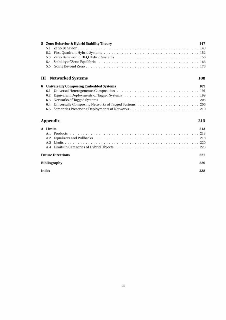
1.1.14 Natural transformations between contravariant functors. If F,G : C → D are contravariant
functors, then a natural transformation τ : F→ D between these functors is again a collection of mor-
11
Hybrid Objects
F (A)τA- G(A)
F (B)
F ( f )
? τB- G(B)
G( f )
?
F (A)τA- G(A)
F (B)
F ( f )6
τB- G(B)
G( f )6
F covariant, G covariant F contravariant, G contravariant
F (A)τA- G(A)
F (B)
F ( f )
? τB- G(B)
G( f )6
F (A)τA- G(A)
F (B)
F ( f )6
τB- G(B)
G( f )
?
F covariant, G contravariant F contravariant, G covariant
Table 1.2: Different variations of natural transformations.
phisms τA : F (A) →G(A), except we now require that for every f : A → B in C the following diagram:
F (A)τA- G(A)
F (B)
F ( f )6
τB- G(B)
G( f )6
commutes. Natural transformations also can be defined when considering mixed covariant/contravariant
functors as illustrated in Table 1.2.
1.1.15 Diagrams. A diagram (or J-diagram) in a category C is a functor F : J→ C for some small cate-
gory J (an indexing category). We can form the category of all J-diagrams in the category C, denoted by
CJ, with
Objects: Functors F : J→C,Morphisms: Natural transformations.
Categories of this form are commonly referred to as functor categories.
1.1.16 The constant functor. A very important, yet simple, functor is the constant functor, ∆J. This is
a functor:
∆J : C→CJ,
given on objects A ∈Ob(C) by
∆J(A)(a) = A∆J(A)(α) = idA- ∆J(A)(b) = A
for α : a → b in J. On morphisms f : A → B in C, ∆J( f )a := f for every object a of J.
12
Hybrid Objects
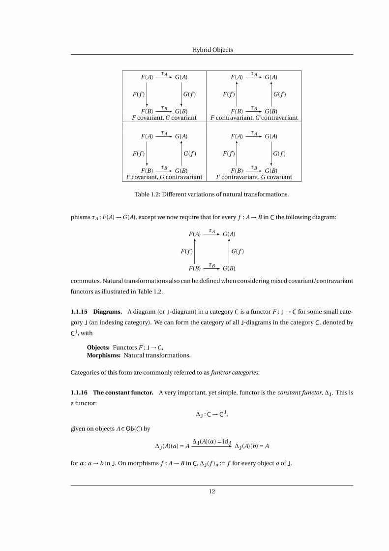
1.1.17 Basic diagrams. Diagrams play a central role in the theory of hybrid objects, except we will
restrict our attention to a specific class of small categories termed D-categories. In preparation, we now
enumerate some of the basic diagrams of interest in category theory.
(•): A category consisting of a single object and an identity morphism. A functor F : (•) → Ccan be identified with an object of C, i.e., it is just the object F (•) ∈ Ob(C). Therefore, thecategory C(•) =Ob(C).
(•→ •): A category consisting of two objects, the identity morphisms for these objects and anon-identity morphism. A functor
F : (•→•) →C
is just a diagram:
F (•→•) = Af - B
in C. Therefore, the category C(•→•) can be identified with the morphisms in C.(•→→•): A category with two objects and two non-identity morphisms. A functor
F : (•→→•) →C
is just a diagram:
F (•→→•) = Af1-
f2
- B
in C. Diagrams of this form are important when considering equalizers and coequalizers.(•←•→•): A category with three objects and two non-identity morphisms. A functor
F : (•←•→•) →C
is just a diagram:
F (•←•→•) = A fB
g- C
in C. Diagrams of this form are important when considering pushouts.(•→•←•): A category with three objects and two non-identity morphisms. A functor
F : (•→•←•) →C
is just a diagram:
F (•→•←•) = Af - B g
C
in C. Diagrams of this form are important when considering pullbacks.
1.2 D-categories
In this section, we introduce an important class of small categories: D-categories. These cate-
gories are very simple small categories that essentially can be thought of as graphs. In fact, we will demon-
strate that the category of (oriented) D-categories is isomorphic to the category of (oriented) graphs:
Dcat∼=Grph .
13

Hybrid Objects
The proof of this fact is constructive in nature, i.e., it is shown how to obtain a graph from a D-category
and a D-category from a graph.
The motivation for considering D-categories is that they play a fundamental role in defining
hybrid objects over a category. The motivation for the name D-categories is that they define the “discrete”
structure of a hybrid object over a category.
1.2.a Axioms and Orientations
We must define a specific type of small category, termed a D-category, in order to introduce
hybrid objects. This is a small category in which every diagram has the form:
• • •
• •-
•-
· · · • •-
That is, a D-category has as its basic atomic unit a diagram of the form:
•
• •-
and any other diagram in this category must be obtainable by gluing such atomic units along the codomain
of a morphism (and not the domain). More formally, consider the following:
Definition 1.6. A D-category is a small category D satisfying the following two axioms:
AD1 Every object in D is either the domain of a non-identity morphism in D or the codomain of a non-
identity morphism but never both, i.e., for every diagram
a0α1- a1
α2- · · · αn- an
in D, all but one morphism must be the identity (the longest chain of composable non-identity
morphisms is of length one).
AD2 If an object in D is the domain of a non-identity morphism, then it is the domain of exactly two
non-identity morphisms, i.e., for every diagram in D of the form
a0
a1
α1
a2
α 2
a3
α
3
· · · · · · · · ·an
αn -
consisting of all morphisms with domain a0, either all of the morphisms are the identity or two and
only two morphisms are not the identity.
Remark 1.2. We could form the category of D-categories with objects D-categories and morphisms all
functors. This being said, we actually do not consider this category as it does not yet have enough struc-
ture, i.e., we will consider D-categories that are oriented and functors between D-categories that preserve
these orientations.
14

Hybrid Objects
Example 1.8. An example of a D-category is given in the following diagram:
•
• •
•
-•
-
•
-
•
•
-
•
•-
•
• •
•
-
-
•
•-
This D-category can be justifiably thought of as a “cycle” D-category.
1.2.1 Important objects in D-categories. Let D be a D-category. We use Mor(D) to denote the mor-
phisms of D, i.e.,
Mor(D) = ⋃(a,b)∈Ob(D)×Ob(D)
HomD(a, b),
and Morid (D) to denote the set of non-identity morphisms of D, i.e.,
Morid (D) = α ∈Mor(D) :α 6= id.
For a morphism α : a → b in D, recall from Definition 1.1 that its domain is denoted by dom(α) = a and its
codomain is denoted by cod(α) = b.
For D-categories, there are two sets of objects that are of particular interest; these are subsets of
Ob(D). The first of these is termed the edge set of D, denoted by E(D), and defined to be:
E(D) = a ∈Ob(D) : a = dom(α), a = dom(β), α,β ∈Morid (D), α 6=β.
That is, for all a ∈ E(D) there are two and only two morphisms (which are not the identity) α,β ∈Mor(D)
such that a = dom(α) and a = dom(β), so we denote these morphisms by sa and ta (the specific choice will
define an orientation). Conversely, given a morphism γ ∈ Morid (D), there exists a unique a ∈ E(D) such
that γ= sa or γ= ta . Therefore, every object a ∈E(D) sits in a diagram of the form:
dom(sa) = a = dom(ta)
b = cod(sa)
sa
cod(ta) = c
ta
-(1.2)
15

Hybrid Objects
Note that giving all diagrams of this form (for which there is one for each a ∈E(D)) gives all the objects in
D, i.e., every object of D is the domain or codomain of sa or ta for some a ∈E(D).
Define the vertex set of D by:
V(D) = (E(D))c ,
where here (E(D))c is the complement of E(D) in the set Ob(D). It follows by definition that
E(D)∩V(D) = ;,
E(D)∪V(D) = Ob(D).
The above choice of morphisms sa and ta can be used to define an orientation on a D-category.
Figure 1.1: The edge and vertex sets for a D-category.
Example 1.9. For the D-category introduced in Example 1.8, the edge and vertex sets can be seen in Figure
1.1; in this figure “•” is now just an object, not an object together with its identity morphism.
Definition 1.7. An orientation of a D-category D is a pair of functions (s,t) between sets:
E(D)s-
t- Morid (D),
16

Hybrid Objects
that fit into a diagram
E(D)
E(D)s-
t-
id-
Morid (D)
dom
6
V(D)
cod
?
(1.3)
in which the top triangle commutes.
Notation 1.2. We will always assume that a given D-category has an orientation. Therefore, we will not
explicitly say “oriented D-category” since all D-categories considered will be oriented.
The notion of a D-category, together with an orientation thereon, can be summarized succinctly
as follows:
Definition 1.8. A D-category is a small category D such that:
¦ There exist two subsets of Ob(D), E(D) and V(D), termed the edge set and vertex set, satisfying:
E(D)∩V(D) = ;,
E(D)∪V(D) = Ob(D),
¦ There exists a pair of functions:
E(D)s-
t- Morid (D),
such that:
s(E(D))∩ t(E(D)) = ;,
s(E(D))∪ t(E(D)) = Morid (D).
and the diagram in (1.3) is well-defined and commutes; the pair (s,t) is termed an orientation of D.
Remark 1.3. By requiring that the diagram in (1.3) is well-defined we are imposing the condition that
dom(Morid (D)) =E(D) and cod(Morid (D)) =V(D). In addition, for every a ∈E(D), there is a correspond-
ing diagram (1.2) in which b, c ∈V(D).
To verify that the (oriented) D-categories, as defined in 1.8, satisfy the axioms of a D-category as
given in Definition 1.6, we demonstrate the following:.
Lemma 1.1. A D-category, as defined in 1.8, satisfies AD1 and AD2.
17

Hybrid Objects
Proof. Beginning with AD1, we argue by way of contradiction. Suppose that there are two morphisms
aα - b
β - c
with α 6= id and β 6= id. Then, since s(E(D))∪ t(E(D)) = Morid (D), α = sa or ta and β = sb or tb . Since
b = cod(α), and because (1.3) is well-defined, it follows that b ∈ V(D). But b = dom(β) and so, again
because of the fact that (1.3) is well-defined, it follows that b ∈ E(D). Since E(D)∩V(D) = ; we have
established the desired contradiction.
To show that AD2 holds, let a = dom(α) with α 6= id. Then a ∈ E(D) by the fact that (1.3) is
well-defined; moreover a = dom(sa) and a = dom(ta) by the commutativity of this diagram. Therefore,
a is the domain of two non-identity morphisms. Now, for any other non-identity morphism β such that
a = dom(β), since s(E(D))∪t(E(D)) =Morid (D), it follows that β= sa or β= ta . Therefore, a is the domain
of exactly two non-identity morphisms.
Example 1.10. We can pick an orientation for the D-category given in Example 1.8. This orientation is
displayed in the following diagram:
a1
a8 a2
b1
sa1
ta8-
b2
ta1
- sa2
b8
sa8 -
b3
ta2
a7
ta7 -
a3
sa3
b7sa7
-b4
ta3
b6 b5
a6
ta6
-
sa6
-
a4
sa4
ta4
a5
sa5
-
ta5
This is by no means the only orientation that we could impose; it was chosen because it makes this D-
category into a “directed cycle” D-category or a D-cycle. D-categories of this form will be fundamental in
the study of Zeno behavior in hybrid systems (cf. Chapter 5).
1.2.2 The category of D-categories. Define the category of (oriented) D-categories, Dcat, to have ob-
jects D-categories. A morphism between two D-categories, D and D′ (with orientations (s,t) and (s′,t′),
respectively) is a functor ~F : D →D′ such that
~F (E(D)) ⊆E(D′), ~F (V(D)) ⊆V(D′), (1.4)
18

Hybrid Objects
and the following diagrams
E(D)~F - E(D′) E(D)
~F - E(D′)
Morid (D)
s
? ~F- Morid (D′)
s′
?Morid (D)
t
? ~F- Morid (D′)
t′
?
(1.5)
commute. By requiring these diagrams to commute, it implies that for all diagrams of the form:
a
b
sa
c
ta
-
in D, i.e., a ∈E(D) and b, c ∈V(D), there are corresponding diagrams:
~F (a)
~F (b)
~F (sa) = s′~F (a)
~F (c)
~F (ta) = t′~F (a)
-
in D′, where ~F (a) ∈E(D′) and ~F (b), ~F (c) ∈V(D′).
Example 1.11. Let D and D′ be the D-categories given by the following diagrams:
a
D =
b1
sa
b2
ta
-
a′
D′ =
b′
s′a′
?
t′a′
?
There is a morphism ~F : D →D′ of D-categories given by:
~F (a) = a′, ~F (b1) = ~F (b2) = b′, ~F (sa) = s′a′ , ~F (ta) = t′a′ .
This morphism can be visualized by the following diagram:
a
D
b1
sa
b2
ta
-
a′?
...........................................
D′
~F
?
b′
s′a′
?
t′a′
?......
........
........
........
........
........
........
........
........
.........................................................................-
19

Hybrid Objects
Example 1.12. Let D′′ be the D-category given by the following diagram:
a1 a2
D′′ =
b1
sa1
b2
sa2
ta1
-
b3
ta2
-
In this case, there is not a morphism from D′′ to D as any such morphism would not preserve the orienta-
tions of these D-categories.
1.2.3 Elementary properties. At this point, we verify some elementary properties of D-categories.
Lemma 1.2. For any two objects a, b in D, if a ∼= b then a = b.
Proof. We argue by contradiction. If a ∼= b and a 6= b, then there exist two non-identity morphisms:
aα - b
α−1- a.
This violates AD1.
Using this result, we characterize equivalences between D-categories.
Lemma 1.3. A morphism ~F : D →D′ is an equivalence of categories iff it is an isomorphism of categories.
1.2.b D-categories and Graphs
We now turn our attention to relating D-categories to graphs.
1.2.4 Oriented graphs. A (directed or oriented) graph is a pair Γ = (Q,E), where Q is a set of vertices
and E is a set of edges (assumed to be disjoint), together with a pair of functions:
Esor -
tar- Q
called the source and target functions; for e ∈ E , sor(e) is the source of e and tar(e) is the target of e.
A morphism of graphs is a pair F = (FQ ,FE ) : Γ = (Q,E) → Γ′ = (Q′,E ′), where FQ : Q → Q′ and
FE : E → E ′, such that the following diagrams commute:
EFE - E ′ E
FE - E ′
Q
sor
? FQ - Q′
sor′
?Q
tar
? FQ - Q′
tar′
?
(1.6)
Thus we have defined the category of graphs, Grph.
20

Hybrid Objects
Example 1.13. An example of a graph is given by the following directed cycle graph:
1e1 - 2
8
e8 -
3
e2-
7
e7
6
4
e3
?
6 e5
e6
5
e4
A graph of this form is often denoted by C8.
1.2.5 D-categories from graphs. Given a graph, Γ= (Q,E), we can associate to this graph a D-category
DΓ. Define the objects of DΓ by defining
E(DΓ) := E , V(DΓ) :=Q, Ob(DΓ) =E(DΓ)∪V(DΓ).
To define the morphisms of DΓ we define, for every e ∈ E , morphisms:
e
sor(e)
se
tar(e)
te
-
We complete the description of DΓ by defining an identity morphism on each object of DΓ. Note that in
the definition of DΓ, we gave it a canonical orientation; namely, (s,t) where se and te are defined as above
for every e ∈ E .
Given a morphism F = (FQ ,FE ) : Γ→ Γ′, we can define a functor ~F : DΓ → DΓ′ by defining it on
objects and morphisms as follows:
~F (a) := FE (a) if a ∈E(DΓ)
FQ(a) if a ∈V(DΓ)~F (γ) :=
s′~F (e)
if γ= se
t′~F (e)if γ= te
Of course, ~F is defined on identity morphisms in the obvious fashion: ~F (ida) := id~F (a). It follows by the
commutativity of (1.6) that ~F is a valid morphism of D-categories.
The method of associating a D-category to a graph defines a functor:
dcat : Grph→Dcat
We will introduce the inverse of this construction, but first consider the following:
Example 1.14. The D-category obtained from the graph C8 is just the D-category given in Example 1.10.
To make explicit the fact that this D-category is obtained from the graph C8, we could denote it by DC8 ,
21

Hybrid Objects
and label its objects and morphisms as follows:
e1
e8 e2
1
se1
te8-
2
te1
- se2
8
se8 -
3
te2
e7
te7-
e3
se3
7se7
-4
te3
6 5
e6
te6
-
se6
-
e4
se4
te4
e5
se5
-
te5
This is in accordance with the construction given in the previous paragraph.
1.2.6 Graphs from D-categories. Given a D-category D, we can obtain a graph from this D-category,
ΓD = (QD ,ED) := (V(D),E(D)),
with source and target functions:
ED
sor= cod(s(− ))-
tar= cod(t(− ))- QD
For a morphism between D-categories, ~F : D → D′, we obtain a morphism between the graphs ΓD and
ΓD′ :
F := (~F |QD, ~F |ED
) = (~F |V(D), ~F |E(D)).
It follows that F is a valid morphism of graphs; (1.6) commutes because (1.5) commutes.
The result of these constructions is a functor:
grph : Dcat → Grph .
Example 1.15. The graph obtained from the D-category given in Example 1.10 is just the graph C8. To
make explicit that this graph was obtained from this D-category, we could label the vertices and edges of
22

Hybrid Objects
this graph as follows:
b1a1 - b2
b8
a8-
b3
a2-
b7
a7
6
b4
a3
?
b6 a5
a6
b5
a4
This is in accordance with the construction given in the previous paragraph.
We now introduce a very important, although fairly obvious, result. Its importance lies in the fact
that many of the properties that the category of graphs displays—which is a fair number—the category of
D-categories will inherit. This will be made explicit, for example, in Appendix A
Theorem 1.1. There is an isomorphism of categories:
Dcat∼=Grph,
where this isomorphism is given by the functor grph : Dcat→Grph with inverse dcat : Grph→Dcat.
Proof. We first verify that dcatgrph = IdDcat. On objects, this holds since
Morid (dcatgrph(D)) = se e∈ED∪ te e∈ED
= se e∈E(D) ∪ te e∈E(D) =Morid (D),
Ob(dcatgrph(D)) = ED ∪QD =V(D)∪E(D) =Ob(D),
and the identity morphisms of D and dcat grph(D) are the same by definition. Consider a morphism
~F : D →D′ of D-categories. For all a ∈Ob(D),
dcatgrph(~F )(a) = ~F (a) if a ∈ ED =E(DΓD
) =E(D)
~F (a) if a ∈QD =V(DΓD) =V(D)
= ~F (a),
and for all γ ∈Mor(D),
dcatgrph(~F )(γ) = s′
~F (a)if γ= sa
t′~F (a)if γ= ta
= ~F (γ) if γ= sa
~F (γ) if γ= ta
= ~F (γ).
Therefore dcatgrph = IdDcat.
23

Hybrid Objects
Next we verify that grphdcat = IdGrph. For a graph Γ= (Q,E), we have
grphdcat(Γ) = ΓDΓ= (QDΓ
,EDΓ) = (V(DΓ),E(DΓ)) = (Q,E) = Γ.
For a morphism of graphs F = (FQ ,FE ) : Γ→ Γ′,
grphdcat(F )Q = ~F |Q = FQ , grphdcat(F )E = ~F |E = FE .
1.3 Hybrid Objects
The starting point for theory of hybrid objects is the observation that systems that display both
continuous and discrete behavior, i.e., hybrid systems, can be represented by a D-category together with
a functor. This relates hybrid systems to the two most fundamental objects in category theory: a functor
and a natural transformation.
In this section, and from this point on, we will denote D-categories by the calligraphic symbols:
A , B, C , et cetera.
Using the notion of a D-category, we have the following definition of a hybrid object over a
category.
Definition 1.9. Let C be a category. A hybrid object over C is a pair (A ,A), where A is a D-category and
A : A →C
is a (covariant) functor.
For a hybrid object (A ,A) over C, the category C is called the target category, the functor A is
called the continuous component of the hybrid object, and the category A is called its discrete component.
Notation 1.3. We denote the value of a functor A : A → C on objects and morphisms of A by Aa and
Aα, i.e., Aa = A(a) and Aα = A(α). This is done to notationally differentiate the “continuous” portion of a
hybrid object from other functors.
Example 1.16. A (real) hybrid vector space is a hybrid object (V ,V) over VectR, i.e.,
V : V →VectR .
In particular, Va is a vector space for every object a of V and Vα : Va → Vb is a linear map for everyα : a → b
in V .
Having defined hybrid objects, there is a natural definition of morphisms between hybrid ob-
jects.
24

Hybrid Objects
Definition 1.10. Let (A ,A) and (B,B) be two hybrid objects over the category C. A morphism of hybrid
objects, or just a hybrid morphism, is a pair
(~F , ~f ) : (A ,A) → (B,B), (1.7)
where ~F : A →B is a morphism in Dcat and ~f is a natural transformation
~f : A→ B ~F (1.8)
in CA .
A morphism (~F , ~f ) : (A ,A) → (B,B) of hybrid objects can be visualized in the following diagram:
A
A -~f ↓.
B ~F- C
B
B
-
~F
-
and has, like a hybrid object, both a discrete and a continuous component, which justifies the term “hy-
brid morphism.” The discrete component is given by the functor ~F : A →B, and the continuous compo-
nent is given by the natural transformation ~f .
As morphisms of hybrid objects play a central role, we devote some energy to discussing their
meaning. First, we introduce some notation and examples.
Notation 1.4. Often, hybrid objects are simply denoted by
A : A →C .
It is clear that the corresponding hybrid object is the pair (A ,A). We will often only be interested in a
single hybrid object and its relation to hybrid objects with the same discrete structure, i.e., the same D-
category. In this case, we will denote such a hybrid object by A and a morphism between it and another
hybrid object, B, by ~f : A→ B; that is, A represents the hybrid object (A ,A), B represents the hybrid object
(A ,B) and ~f represents the hybrid morphism (~IdA , ~f ), where ~IdA is the identity functor (or the identity
morphism of A in Dcat).
Example 1.17. Consider the D-categories A and B given by the following diagrams:
a
A =
b1
sa
b2
ta
-
a′
B =
b′
s′a′
?
t′a′
?
Let ~F : A →B be the morphism of D-categories given in Example 1.11.
25

Hybrid Objects
For A : A →C and B : B →C, which can be visualized in the following diagrams:
Aa
A(A ) =
Ab1
Asa
Ab2
Ata
-
Ba′
B(B) =
Bb′
Bs′a′
?
Bt′a′
?
A morphism ~f : A→ ~F∗(B) in CA consists of three morphisms ~fa , ~fb1 and ~fb2 in C such that the following
diagram
Aa
A
Ab1
Asa
Ab2
Ata
-
Ba′
~fa
?
~F∗(B)
~f
?
Bb′
~fb1
?
Bs′a′
Bb′
~fb2
?
Bt′a′
-
commutes. The end result is a morphism of hybrid objects: (~F , ~f ) : (A ,A) → (B,B).
Example 1.18. For two hybrid vector spaces (V ,V) and (V ′,V′), a hybrid morphism between these hybrid
objects consists of a functor ~F : V → V ′ between their discrete components and a hybrid linear map, i.e.,
natural transformation:
~f : V→ V′ ~F .
That is, for every α : a → b in V , there is a commuting diagram:
Va
~fa- V~F (a)
Vb
Vα
? ~fb- V~F (b)
V~F (α)
?
where ~fa and ~fb are linear maps.
Morphisms of hybrid objects can be defined in an equivalent and possible more enlightening
way through the use of pullbacks of functors.
1.3.1 Pullbacks. The pullback of a functor ~F : A →B is a functor:
~F∗ : CB →CA
26

Hybrid Objects
given on objects, i.e., functors B : B → C, and morphisms, i.e., natural transformations ~g : B→ B′, of CB
by:
~F∗(B) = B ~F , ~F∗(~g ) = ~g ~F ,
where ~F∗(~g ) is the natural transformation given on objects a of A by
(~F∗(~g ))a = ~g~F (a) : B~F (a) → B′~F (a)
.
This implies that for a morphism of hybrid objects (1.7),
~f : A→ ~F∗(B),
which is simply a reformulation of (1.8). This is the notation we will most frequently use.
1.3.2 Composing hybrid morphisms. Given two hybrid morphisms (~F , ~f ) : (A ,A) → (B,B) and (~G , ~g ) :
(B,B) → (C ,C), the composite morphism is given by:
(~G , ~g ) (~F , ~f ) := (~G ~F , ~F∗(~g )• ~f ) : (A ,A) → (C ,C).
Specifically, the composite morphism is just the standard composition of functors and objectwise com-
position of natural transformations, i.e.,
~F∗(~g )• ~f : A→ (~G ~F )∗(C) = ~F∗(~G∗(C)),
in CA is defined objectwise by (~F∗(~g )• ~f )a = ~F∗(~g )a ~fa = ~g~F (a) ~fa .
1.3.3 Decomposing hybrid morphisms. Every morphism (~F , ~f ) : (A ,A) → (B,B) has a canonical fac-
torization:
(A ,A)(~F , ~f ) - (B,B)
(A , ~F∗(B))
(~F , ~F∗(~idB))
-
(~IdA , ~f ) -
into its continuous and discrete component.
1.3.4 Categories of hybrid objects. Utilizing hybrid objects and hybrid morphisms, we have the fol-
lowing:
Definition 1.11. Let C be a category. The category of hybrid objects over the category C, denoted by
Hy(C), has as
Objects: Hybrid objects over C, i.e., pairs (A ,A), where A : A →C.Morphisms: Morphisms of hybrid objects, i.e., pairs
(~F , ~f ) : (A ,A) → (B,B),
where ~F : A →B is a morphism in Dcat and ~f : A→ ~F∗(B) is a morphism in CA .
27

Hybrid Objects
It is useful to know that the collection of morphisms between any two objects in Hy(C) form a
set. This makes Hy(C) a category in the classical sense.
Lemma 1.4. For any two objects (A ,A) and (B,B) of Hy(C), HomHy(C)((A ,A), (B,B)) forms a set.
Proof. Since HomCat(A ,B) is a set and
HomDcat(A ,B) ⊆HomCat(A ,B),
it follows that HomDcat(A ,B) is a set. Moreover, HomCA (A, ~F∗(B)) form sets for any ~F ∈HomDcat(A ,B).
So
HomHy(C)((A ,A), (B,B)) ⊆HomDcat(A ,B)×( ⋃~F∈HomDcat(A ,B)
HomCA (A, ~F∗(B))
)
is a set.
Example 1.19. We already have introduced the notion of a hybrid vector space. The collection of all
hybrid vector spaces forms the category of hybrid vector spaces: Hy(VectR).
1.3.5 Left comma categories. The notion of a hybrid object over a category has not yet appeared in the
literature as it was originally formulated by the author. There is a notion that is “close” to this one, that of a
left comma category (as introduced by Saunders Mac Lane [74], where is was referred to as a super comma
category4), and it in fact supports the terminology “hybrid object over a category.” We briefly discuss left
comma categories, comparing and contrasting them to categories of hybrid objects.
Let C be a category. The left comma category (Cat ·↓·C) is a category with
Objects: Pairs (A, A), where A is a small category and A : A→C is a functor,
Morphisms: Pairs (F, f ) : (A, A) → (B,B), where F : A → B is a functor and f : B F→ A is a
natural transformation.
If we consider the left comma category (Dcat ·↓·C), then this category has as
Objects: Pairs (A ,A) where A is a small category and A : A →C is a functor,
Morphisms: Pairs (~F , f ) : (A ,A) → (B,B) where ~F : A →B is a functor and f : B ~F → A is anatural transformation.
This is “almost” the category of hybrid objects over C, except the direction of the natural transformations
are reversed, i.e.,
f : B ~F → A for (Dcat ·↓·C) f : A→ B ~F for Hy(C).
This is a not-so-subtle difference that has important ramifications. We only note that the motivation for
considering categories of hybrid objects rather than left comma categories can be seen when the notion
of a trajectory is introduced in Section 2.3.
4We avoid the name “super comma category” since there is an entire area of “super” mathematics and we want to prevent thepossibility of confusion.
28

Hybrid Objects
1.3.6 Pushforwards. Consider a functor G : C→D. For a D-category A , this induces a functor:
G∗ : CA →DA
given on objects, i.e., functors A : A →C by
G∗(A) =G A.
This functor can be visualized as follows:
A
C
A
? G - D
G∗(A)
-
From a natural transformation ~f : A→ A′ in CA , we obtain a natural transformation:
G∗(~f ) : G∗(A)→G∗(A′)
defined objectwise by: G∗(~f )a :=G(~fa) : G(Aa) →G(A′a). The relationship between pushforwards and pull-
backs is given as follows:
Lemma 1.5. For G : C→D and ~F : A →B, the following diagram
CB G∗- DB
CA
~F∗
?G∗- DA
~F∗
?
(1.9)
commutes.
Proof. For B : B →C,
~F∗(G∗(B)) = ~F∗(G B) =G B ~F =G ~F∗(B) =G∗(~F∗(B)).
For ~g : B→ B′ in CB , it is enough to check that the commutativity condition holds objectwise:
~F∗(G∗(~g ))a =G∗(~g )~F (a) =G(~g~F (a)) =G(~F∗(~g )a) =G∗(~F∗(~g ))a .
1.3.7 Functors between categories of hybrid objects. Consider a functor G : C→D between two cate-
gories. Using the pushforward of the functor G , this induces a functor:
Hy(G) : Hy(C) →Hy(D)
29

Hybrid Objects
between categories of hybrid objects. On objects (A ,A) and morphisms (~F , ~f ) : (A ,A) → (B,B) of Hy(C),
the functor Hy(G) is given by:
Hy(G)(A ,A) = (A ,G∗(A)),
Hy(G)(~F , ~f ) = (~F ,G∗(~f )) : (A ,G∗(A)) → (B,G∗(B)),
where G∗(~f ) is well-defined by (1.9).
Example 1.20. Recall from Example 1.6 that there is a forgetful functor U : VectR → Set. This induces a
“forgetful” functor:
Hy(U) : Hy(VectR) →Hy(Set)
between hybrid categories.
1.3.8 Elements of hybrid objects. Consider a set S. We can regard the elements of S as morphisms
from the set with one point, ∗, to S:
S ∼=HomSet(∗,S),
where the isomorphism is given by sending an element s ∈ S to es : ∗→ S with es (∗) := s, and a morphism
e : ∗→ S to e(∗) ∈ S. This inspires the definition of elements of a hybrid object.
Suppose that A : A →C is a hybrid object and C is a category such that there is a forgetful functor
U : C→ Set. Define the elements of (A ,A) by5
ElemHy(C)(A ,A) :=HomSetA (∆A (∗),U∗(A)). (1.10)
So the elements of a hybrid object are natural transformations ~e : ∆A (∗)→U∗(A), i.e., morphisms:
(~IdA ,~e) : (A ,∆A (∗)) → (A ,U∗(A)) =Hy(U)(A ,A),
in Hy(Set). In particular, for ~e ∈ ElemHy(C)(A ,A), the following diagram must commute:
∗ ~ea- U(Aa)
∗
id∗
? ~eb- U(Ab)
U(Aα)
?
for all α : a → b in A .
By slight abuse of notation, we will identify ~ea with ~ea(∗) ∈ Aa ; with this notation, we write ~e ∈(A ,A). Note that ~e ∈ (A ,A) must satisfy the following properties:
¦ ~ea ∈ Aa for all objects a of A ,
¦ ~eb = Aα(~ea) for all α : a → b in A .
5It follows that the elements of a hybrid object form a set, i.e., a hybrid object has a set of elements.
30

Hybrid Objects
Note that ~e inherits the structure of the objects of C objectwise. Therefore, the elements of a hybrid object
can be thought of as “vectors” in an abstract sense of the word; this is one of the motivations for the vector
notation.
Lemma 1.6. If ~f : A→ A′ and ~e ∈ (A ,A) then ~f (~e) ∈ (A ,A′) where ~f (~e)a := ~fa(~ea).
Proof. It trivially follows that ~f (~e)a ∈ A′a . The second condition follows from the fact that:
A′α(~f (~e)a) = A′
α(~fa(~ea)) = ~fb(Aα(~ea)) = ~fb(~eb) = ~f (~e)b .
Example 1.21. Let (V ,V) be a hybrid vector space. A hybrid vector is an element of this hybrid object:
~v ∈ (V ,V).
In particular, a hybrid vector must satisfy the following properties:
¦ ~va ∈ Va for all objects a of V , i.e., ~va is a vector,
¦ ~vb = Vα(~va) for all α : a → b in V .
In fact, we can justify the use of the term hybrid vector since we have two operations: hybrid
vector addition and hybrid scalar multiplication. These are operations:
ElemHy(VectR)(V ,V)×ElemHy(VectR)(V ,V) → ElemHy(VectR)(V ,V)
(~v, ~w) 7→ ~v + ~w
R×ElemHy(VectR)(V ,V) → ElemHy(VectR)(V ,V)
(r,~v) 7→ r~v
defined objectwise by (~v+ ~w)a := (~va+ ~wa) and (r~v)a := r~va . It follows from the additivity and homogeneity
of linear maps that ~v + ~w and r~v are again hybrid vectors.
More generally, the set of elements of a hybrid vector space, ElemHy(VectR)(V ,V), is again a vec-
tor space. The vector addition identity element is given by ~0 which is defined objectwise ~0a = 0Va where
0Va is the vector addition identity element for Va . Similarly, there is a scalar multiplication identity ele-
ment~1. The axioms of a vector space are easy to verify since they hold objectwise.
1.4 Cohybrid Objects
Thus far, we have only considered covariant functors. Contravariant functors will also arise nat-
urally in a hybrid setting as they naturally arise in category theory. In order to deal with these functors in
a systematic fashion, we introduce categories of cohybrid objects. First, we discuss:
31

Hybrid Objects
1.4.1 Covariant functor categories. For a category C, we use A C to denote the category of contravari-
ant functors A : A → C, with morphisms natural transformations between contravariant functors (see
Paragraph 1.1.14). Given a morphism ~F : A →B of D-categories, it induces a morphism of contravariant
functor categories:
~F∗ : BC→A C.
Given a covariant functor G : C→D, there is a corresponding covariant functor:
G∗ : A C→A D
for every D-category A . Similarly, if G is contravariant, it induces functors:
G∗ : A C→DA , G∗ : CA →A D.
In all cases ~F∗ G∗ =G∗ ~F∗.
Definition 1.12. Let C be a category. The category of cohybrid objects over the category C, denoted by
CoHy(C), is given by:
Objects: Cohybrid objects over C, which are pairs (A ,A) where A is a D-category and A is acontravariant functor A : A →C.
Morphisms: Pairs (~Fop, ~f ) : (A ,A) → (B,B) where
¦ ~Fop : A →B is the morphism in Dcatop corresponding to the morphism ~F : B →A
in Dcat,
¦ ~f : ~F∗(A)→ B in BC.
1.4.2 Relating categories of hybrid and cohybrid objects. The numerous morphisms in the different
categories used to define categories of hybrid objects leave a lot of freedom for dualization. To better
understand this, we relate categories of hybrid and cohybrid objects.
Specifying a contravariant functor A : A →C is equivalent to specifying a covariant functor Aop :
A →Cop given by:
Aop(
aα - a′
)= Aop
a = AaAopα = (Aα)op- Aop
a′ = Aa′ .
Therefore, the objects of CoHy(C) are in bijective correspondence with the objects of Hy(Cop) and hence
the objects of Hy(Cop)op.
For a morphism (~Fop, ~f ) : (A ,A) → (B,B) of cohybrid objects, ~f : ~F∗(A)→ B in BC. That is, for
every β : b → b′ in B, there is a corresponding commuting diagram:
A~F (b)
~fb - Bb
A~F (b′)
A~F (β)
6
~fb′- Bb′
Bβ
6
32

Hybrid Objects
in C. Taking opposites yields a commuting diagram:
Aop~F (b)
~f opb Bop
b
Aop~F (b′)
Aop~F (β)
?
~f opb′
Bopb′
Bopβ
?
in Cop. Therefore, ~f op : Bop → ~F∗(Aop) in CB and associated to (~Fop, ~f ) in CoHy(C) is a morphism
(~F , ~f op) : (B,Bop) → (A ,Aop)
in Hy(Cop). Since the direction of (~Fop, ~f ) and (~F , ~f op) are opposite to one another, we conclude that:
Proposition 1.1. For every category C,
CoHy(C) ∼=Hy(Cop)op.
The motivation for considering categories of cohybrid objects is that they arise naturally in the
context of contravariant functors. That is, the functors induced from contravariant functors are functors
between categories of hybrid objects and categories of cohybrid objects.
1.4.3 Contravariant functors and categories of hybrid objects. Let G : C→D be a contravariant func-
tor between two categories. This induces a contravariant functor:
Hy(G) : Hy(C) →CoHy(D).
This functor is given on objects (A ,A) and morphisms (~F , ~f ) : (A ,A) → (B,B) of Hy(C) by:
Hy(G)(A ,A) := (A ,G∗(A)),
Hy(G)(~F , ~f ) := (~Fop,G∗(~f )) : (B,G∗(B)) → (A ,G∗(A)),
where ~Fop : B →A is the morphism in Dcatop corresponding to the morphism ~F : A →B in Dcat.
Similarly, there is a contravariant functor:
CoHy(G) : CoHy(C) →Hy(D),
defined in an analogous manner. Finally, if G is covariant then there is a covariant functor:
CoHy(G) : CoHy(C) →CoHy(D)
defined in a manner analogous to the induced functor given in Paragraph 1.3.7.
Example 1.22. The functor that associates to a vector space its dual:
( − )? : VectR→VectR
33

Hybrid Objects
induces a contravariant functor:
Hy(( − )?) : Hy(VectR) →CoHy(VectR).
In particular, for a hybrid vector space (V ,V), the corresponding cohybrid object
Hy(( − )?)(V ,V) := (V ,V?)
is the dual hybrid vector space to the hybrid vector space (V ,V) and so V? is a contravariant functor:
V? : V →VectR .
This motivates the terminology “cohybrid object.”
1.4.4 Elements of cohybrid objects. Suppose that A : A →C is a cohybrid object, i.e., A is a contravari-
ant functor, and C is a category such that there is a forgetful functor U : C → Set. This yields a covariant
functor CoHy(U) : CoHy(C) →CoHy(Set) where CoHy(U)(A ,A) := (A ,U∗(A)).
As with hybrid objects, define the elements of (A ,A) by
ElemCoHy(C)(A ,A) :=HomA Set(∆opA
(∗),U∗(A)), (1.11)
where ∆opA
is the contravariant constant functor defined in the obvious manner. Therefore, elements of
a cohybrid object are natural transformations ~ω : ∆opA
(∗)→ U∗(A) in A Set, i.e., we have a commuting
diagram:
∗ ~ωa- U(Aa)
∗
id∗6
~ωb- U(Ab)
U(Aα)6
for every α : a → b in A . Therefore, again identifying ~ωa with ~ωa(∗) ∈ Aa and writing ~ω ∈ (A ,A) in this
case, an element ~ω ∈ (A ,A) must satisfy the following properties:
¦ ~ωa ∈ Aa for all objects a of A ,
¦ Aα(~ωb) = ~ωa for all α : a → b in A .
Again, ~ω inherits the structure of the objects of C objectwise.
Example 1.23. For the dual hybrid vector space (V ,V?) to the hybrid vector space (V ,V), an element of
this cohybrid object:
~ω ∈ (V ,V?),
is a hybrid covector.
In particular, it must satisfy the conditions:
34

Hybrid Objects
¦ ~ωa ∈ V?a for all objects a of V , i.e., ~ωa : Va →R is a covector,
¦ V?α(~ωb) = ~ωa , i.e., ~ωb Vα = ~ωa , for all α : a → b in V .
This implies that, for the covariant functor ∆V (R) : V →VectR, a hybrid covector corresponds to a natural
transformation:
~ω : V→∆V (R),
which is the hybrid analogue of the condition that, for a vector space V , a covector is a linear map
w : V →R.
1.5 Network Objects
There is one more important “hybrid” object that will be important when considering net-
worked systems, or networks of systems. These can be thought of as the dual to hybrid objects; their
building block is not D-categories but Dop-categories. While these are just the opposite to D-categories,
we devote some time to their development as they, along with the notion of a category of network objects,
will be fundamental to Chapter 6.
1.5.1 Dop-categories. The opposite of a D-category, or a Dop-category, is given by reversing all of the
arrows in a D-category. Therefore, a Dop-category has the general form:
• • • · · · • •
•-
•-
•-
with its basic atomic unit a diagram of the form:
• •
•-
and any other diagram in this category must be obtainable by gluing such atomic units along the domain
of a morphism (and not the codomain, as was the case for D-categories).
Notation 1.5. In order to differentiate between D-categories and Dop-categories, we denote Dop-categories
by N, i.e., N=N op for some D-category N .
1.5.2 Oriented Dop-categories. Just as with D-categories, Dop-categories can be oriented. All of the
formalisms are the same except that the arrows are reversed. In particular, let N be a Dop-category such
that N=N op. Then
E(N) =E(N ), V(N) =V(N ),
35

Hybrid Objects
since the objects in a category and its opposite category are the same. An orientation of a Dop-category
is obtained from the orientation (s,t) of N , i.e., it is given by (sop,top). That is, an orientation of a Dop-
category is a pair of maps (sop,top) between sets:
E(N)sop -
top- Morid (N)
that fit into a diagram
E(N)
E(N)sop-
top-
id-
Morid (N)
cod
6
V(N)
dom
?
in which the top triangle commutes. Therefore, for every a ∈E(N), there is a diagram in N:
b = dom(sopa ) dom(topa ) = c
cod(sopa ) = a = cod(topa )
topa
sopa -
where b, c ∈V(N).
Morphisms between Dop-categories are defined in a way analogous to morphisms between D-
categories (see 1.2.2). In particular, for ~F : N→M, for every diagram of the form:
b c
a
topa
sopa -
in N, i.e., a ∈E(N) and b, c ∈V(N), there are corresponding diagrams:
~F (b) ~F (c)
~F (a)
~F (topa )
~F (sopa ) -
in M, where ~F (a) ∈E(M) and ~F (b), ~F (c) ∈V(M).
We denote the category of Dop-categories by Dopcat. Note that Dopcat ∼= Dcat, where the iso-
morphism is given by sending N to N with its inverse given by sending N to N.
36

Hybrid Objects
1.5.3 Graphs and Dop-categories. Since Dcat∼=Grph and Dopcat∼=Dcat, it follows that:
Dopcat∼=Grph .
For example, given a graph Γ, the corresponding Dop-category, NΓ, is given by associating to every e ∈ E a
diagram of the form
sor(e) tar(e)
e
tope
sope -
in NΓ. The identity morphisms must be added to each object in NΓ in order to complete the definition.
Example 1.24. The following diagram shows a directed cycle graph, Γ = Ck , and the associated Dop-
category NCk :
e1
ek e2
1e1 - 2 1
sope1
-
topek
2
tope1
sope2-
k
ek -
3
e2-
k
sopek
3
tope2
-
... Ck...
... NCk
...
i +2 i −1 i +2 i −1
i +1 ei
ei+1
i
ei−1
i +1 i
ei+1
topei+1
sopei+1
ei−1
sopei−1
-
topei−1
-
ei
sopei
topei -
1.5.4 Networks over a category. We now define the notion of a network over a category.
Definition 1.13. Let C be a category. The category of networks over the category C, denoted by Net(C),
has as
Objects: Networks over C, which are pairs (N,N) where N is a Dop-category and N is a covari-ant functor N : N→C.
Morphisms: Pairs (~F , ~f ) : (N,N) → (M,M) where
¦ ~F : N→M is the morphism in Dopcat,
¦ ~f : N→ ~F∗(M) in CN.
We refer the reader to Chapter 6 for examples of network objects. Constructions similar to the
cases of categories of hybrid and cohybrid objects also can be introduced, although doing so would be
repetitious.
37

Chapter 2
Hybrid Systems
Hybrid systems effectively describe systems with discrete and continuous behavior; as such,
they are able to model a wide range of phenomena. With this expressiveness comes an increase in com-
plexity; current models are difficult to manipulate as they consist of many different mathematical objects—
a graph, domains, guards, reset maps and vector fields. This presents obvious difficulties in understanding
and analyzing hybrid systems, and so indicates the need for a more coherent mathematical description
of hybrid systems. We claim that the theory of hybrid objects can provide such a description.
We begin by introducing the “standard” model of a hybrid system. The first half of this chapter
is devoted to transforming this standard model, in a constructive manner, into the framework of hybrid
objects, i.e., it is demonstrated how hybrid systems can be viewed categorically. The end result is that a
hybrid system can be represented by a triple:
(M ,M,X),
were (M ,M) is a hybrid manifold, i.e., M : M → Man, and X is a collection of vector fields (indexed by
V(M )) on this hybrid manifold. Therefore, the categorical formulation of hybrid systems is in direct anal-
ogy with dynamical systems, i.e., pairs (M ,X ) where M is a manifold and X is a vector field on that mani-
fold. This analogy is further extended by defining the category of hybrid systems utilizing the category of
dynamical systems.
It is important to consider not only hybrid systems, but how hybrid systems execute or evolve.
The latter half of this chapter is devoted to this topic. We again begin by introducing the “standard” notion
of an execution for a hybrid system, and demonstrate in a constructive fashion how to obtain from this
its categorical analogue. That is, we show that specifying an execution of a hybrid system is equivalent to
specifying a morphism of categorical hybrid systems
(I ,I,d///dt) → (M ,M,X),
where (I ,I,d///dt) is a hybrid system which, roughly speaking, consists of a collection of “intervals” to-
gether with “unit clocks” on these intervals. This again nicely parallels the notion of a trajectory of a
38

Hybrid Systems
dynamical system, which is just a morphism of dynamical systems
(I ,d/dt) → (M ,X ),
with I an interval and d/dt a “unit clock.”
The categorical formulation of hybrid systems and trajectories thereof is fundamental in under-
standing these systems in a broad mathematical context. For example, it is through this formulation of
hybrid systems that we are able to generalize reduction to a hybrid setting and give sufficient conditions
for the existence of Zeno behavior. Without these constructions, these results would have been difficult
to derive. Aside from these results, the categorical formulation of hybrid systems is useful simply because
of the manner in which it simplifies the representation of a hybrid system. We hope that the subsequent
chapters of this dissertation will provide support for these claims.
Related work. There is a wealth of literature on hybrid systems. Instead of providing a complete review
of the subject, we only note that the formulation of the “standard tuple” defining a hybrid systems intro-
duced here is drawn from the series of papers [68, 69, 82, 83, 118, 119]; our definition differs slightly, but
we think that it accurately describes a wide range of hybrid phenomena. Hybrid systems have also been
studied in a categorical context, most notably in [56]. The need for a unifying mathematical framework in
which to study hybrid systems was remarked upon in [103] and [104]; although the constructions in that
work are different than ours, there are many philosophical similarities. Finally, concepts from geometry
are used freely throughout this chapter; we refer the reader to [79] for more on the subject.
The categorical formulation of hybrid systems introduced here first appeared in [14], and has
since appeared in [13, 18].
2.1 Hybrid Systems
This section formally introduces hybrid systems and the corresponding notion of a hybrid space.
We characterize the relationship between hybrid spaces and hybrid manifolds. Utilizing hybrid manifolds,
we define “categorical” hybrid systems and characterize the relationship between these systems and “clas-
sical” hybrid systems. We conclude by introducing the category of hybrid systems. All of these concepts
are illustrated through a series of examples.
Definition 2.1. A hybrid system is a tuple:
H= (Γ,D,G ,R,X ),
where
¦ Γ= (Q,E) is an oriented graph (possibly infinite).
¦ D = Di i∈Q is a set of domains where Di is a smooth manifold.
39

Hybrid Systems
Figure 2.1: The bouncing ball.
¦ G = Ge e∈E is a set of guards, where Ge ⊆ Dsor(e) is an embedded submanifold of Dsor(e).
¦ R = Re e∈E is a set of reset maps; these are smooth maps Re : Ge → Dtar(e).
¦ X = Xi i∈Q is a collection of vector fields, i.e., Xi is a vector field on the manifold Di .
2.1.1 Hybrid spaces. As with dynamical systems, it is sometimes desirable to consider the underlying
“space" of a hybrid system. This amounts to “forgetting" about the vector field on each domain. More
specifically, we can define a (smooth) hybrid space to be a tuple:
H= (Γ,D,G ,R).
It will be seen that hybrid spaces are just hybrid objects over the category of manifolds: hybrid manifolds.
Example 2.1. The quintessential example of a hybrid system is given by the one-dimensional bouncing
ball; see Figure 2.1. While this system has, arguably, been over-studied, we will utilize it in order to illus-
trate non-trivial ideas in a trivial setting.
A ball bouncing in one-dimension is naturally modeled as a hybrid system:
Hball = (Γball,Dball,Gball,Rball,X ball).
That is, we consider a ball dropped from some positive height, say x1, above a surface defined by x1 = 0.
Since the velocity of the ball will reset when it impacts the floor, the graph for this hybrid system is given
by:
Γball = (Qball,Eball), Qball = 1, Eball = e = (1,1).
That is, by a graph of the form:
40

Hybrid Systems
x1
x2Dball1
Gballe
Rballe
Figure 2.2: The hybrid model of a bouncing ball.
Since the phase space of the bouncing ball will consist of two variables, the position x1 and velocity x2,
the domain for the hybrid system is given by:
Dball1 =
x1
x2
∈R2 : x1 ≥ 0
,
and Dball = Dball1 . The guard condition encodes the fact that a transition in the velocities of the system
should occur when the position is zero and the velocity is “downward pointing.” Therefore,
Gballe =
x1
x2
∈R2 : x1 = 0 and x2 ≤ 0
,
and Gball = Gballe . The reset map for the system is given by:
Rballe (x1, x2) =
x1
−r x2
,
where 0 ≤ r ≤ 1 is the coefficient of restitution for the ball; this map encodes the fact that when the ball
impacts the ground, its velocity is reversed and scaled down by the amount of energy lost through impact.
41

Hybrid Systems
Finally, the vector field for this system is given by:
X ball1 (x1, x2) =
x2
−g
,
where g is the acceleration due to gravity. A graphical representation of this system can be seen in Figure
2.2.
Example 2.2. The classical example of a system that models a physical system being controlled is the two
water tanks hybrid system. This system models two tanks that are draining at rates v1 and v2 together with
a spout that is inputting water into one of the two tanks at a rate of w. The control objective is to ensure
that there is water in each tank at all times.
The hybrid system modeling the two water tanks is given by:
Htank = (Γtank,Dtank,G tank,Rtank,X tank).
The graph for the hybrid system, Γtank, is given by:
1e1 -e2
2.
To define the remaining portion of the hybrid system, we consider two state variables, x1 and x2, where
x1 is the level of water in tank 1 and x2 is the level of water in tank 2. Since the goal is to keep the water
in both tanks at all time, we are interested in domains for the hybrid system that capture the fact that the
level of water in each tank must be greater than or equal to zero. Specifically, define Dtank = Dtank1 ,Dtank
2
where
Dtank1 = Dtank
2 =
x1
x2
∈R2 : x1 ≥ 0 and x2 ≥ 0
.
The guard sets for this system should capture the fact that the water spout will switch from one
tank to the other tank if it detects that the other tank is empty. That is, if water is inflowing into tank 1 and
the level of water in tank 2 decreases to 0, i.e., x2 = 0, then the spout should start inflowing water into tank
2. This yields the first guard expression:
G tanke1
=
x1
x2
∈R2 : x1 ≥ 0 and x2 = 0
.
Conversely, if water is inflowing into tank 2 and the system detects that x1 = 0, the spout should switch
from tank 2 to tank 1. This yields the second guard expression:
G tanke2
=
x1
x2
∈R2 : x1 = 0 and x2 ≥ 0
,
and G tank = G tank1 ,G tank
2 .
42

Hybrid Systems
x1
x2
Dtank1
Rtanke1
Rtanke2
Gtanke1
Gtanke2
Dtank2
Figure 2.3: The hybrid model of a two water tank system.
It is assumed that the transition from one tank to the other is made in zero time, so the reset
maps for the system are the identity:
Rtanke1
(x1, x2) = Rtanke2
(x1, x2) = x1
x2
.
Finally, if water is inflowing into the first tank at a rate w, and since water is flowing out of each
tank at a rate of v1 and v2, the ODE governing the system is given by:
X tank1 (x1, x2) =
w − v1
−v2
Similarly, if water is inflowing into the second tank, the resulting dynamics are given by:
X tank2 (x1, x2) =
−v1
w − v2
43

Hybrid Systems
Setting X tank = X tank1 ,X tank
2 completes the description of the hybrid system Htank. This hybrid model can
be seen in Figure 2.3
To make the behavior of the model interesting, we will assume that
maxv1, v2 < w < v1 + v2.
That is, we assume that the inflow is greater than the outflow of each tank, and that the total outflow of
the system is greater than the inflow to the system. This assumption results in Zeno behavior—this type
of behavior will be discussed in detail in Chapter 5, where we will prove that the two water tanks hybrid
system is Zeno (see Example 5.4).
2.1.2 Hybrid manifolds. A (smooth) hybrid manifold is given by a pair (M ,M), where M is a D-category
and M is a functor to the category of smooth manifolds, Man,
M : M →Man . (2.1)
That is, a hybrid manifold is a hybrid object over the category of (smooth) manifolds.
In physical systems, it often is the case that for every a ∈E(M ), and hence every diagram
a
cod(sa)
sa
cod(ta)
ta
-
in M , the corresponding diagram in Man is given by:
Ma
Mcod(sa )
Msa = ı
⊃
Mcod(ta )
Mta
-(2.2)
where Ma ⊆ Mcod(sa ) is an embedded submanifold and Msa = ı is the natural inclusion. We denote hybrid
manifolds of this form by Mııı .
Although we do not explicitly assume that Msa is an inclusion, this often is the case, as the fol-
lowing proposition indicates.
Proposition 2.1. There is a bijective correspondence:
Hybrid Spaces, H= (Γ,D,G ,R) ↔ Hybrid Manifolds, (M ,Mııı ).
Proof. Given a hybrid space H = (Γ,D,G ,R), we define the corresponding hybrid manifold by M(D,G ,R) :
MΓ → Man, where MΓ = dcat(Γ) is the D-category obtained from the graph Γ and M(D,G ,R) is defined for
44

Hybrid Systems
every e ∈E(MΓ) = E by
M(D,G ,R)
e
sor(e)
se
tar(e)
te
-
:=
M(D,G ,R)e :=Ge
M(D,G ,R)sor(e) := Dsor(e)
M(D,G ,R)se
:= ı
⊃
M(D,G ,R)tar(e) := Dtar(e)
M(D,G ,R)te
:= Re
-
It is clear that M(D,G ,R) is a hybrid manifold.
Conversely, consider a hybrid manifold Mııı : M → Man. Let ΓM = grph(M ) = (QM ,EM ) be the
graph obtained from the D-category M . We define
H(M ,Mııı ) = (ΓM ,DMııı ,GMııı ,RMııı ),
where
DMııı := Mıııbb∈V(M )=QM
,
GMııı := Mıııaa∈E(M )=EM
,
RMııı := Mıııta
a∈E(M )=EM.
Example 2.3. The hybrid space for the bouncing ball is given by:
Hball = (Γball,Dball,Gball,Rball).
We will construct the associated hybrid object (M ball,Mball). The D-category associated with the graph
Γball is given by:
a
M ball =
b
sa
?
ta
?
together with the identity morphisms ida : a → a and idb : b → b. The functor
Mball : M ball →Man
takes the following values:
Mball
a
b
sa
?
ta
?
=
Mballa =Gball
e
Mballb = Dball
1
Mballsa
= ı?
∩
Mballta
= Rballe
?
45

Hybrid Systems
x1
x2
Mballa = Gballe
Mballsa = ı
Mballb = Dball
1
Mballta = Rballe
Figure 2.4: The hybrid manifold for the bouncing ball.
A graphical representation of this hybrid manifold can be seen in Figure 2.4
We now see the original motivation for considering D-categories; the edge sets of these cate-
gories serve the purpose of “pulling out the guard.” The claim is that small categories of any other shape
would not allow for the representation of hybrid systems as functors in such a clear fashion.
Example 2.4. The hybrid space for the water tank system is given by:
Htank = (Γtank,Dtank,G tank,Rtank).
We will construct the associated hybrid object (M tank,Mtank). The D-category associated with Γtank is
given by
a1
M tank = b1
sa1
b2
ta1
-
a2
sa2
-
ta2
46

Hybrid Systems
Mtanka2 = Gtanke2
Mtanksa2
= ı
Mtankta2
= Rtanke2
Mtankb1
= Dtank1 Mtank
b2= Dtank
2
Mtankta1
= Rtanke1Mtanksa1
= ı
Mtanka1 = Gtanke1
Figure 2.5: The hybrid manifold for the water tank system.
together with the identity morphisms on each object. The functor
Mtank : M tank →Man
takes the following values:
Mtank(M tank) =
Mtanka1
=G tanke1
Mtankb1
= Dtank1
Mtanksa1
= ı
⊃
Mtankb2
= Dtank2
Mtankta1
= Rtanke1
-
Mtanka2
=G tanke2
Mtanksa2
= ı⊂
-
Mtankta2
= Rtanke2
which completes the description of (M tank,Mtank). This hybrid manifold can be seen in Figure 2.5
47
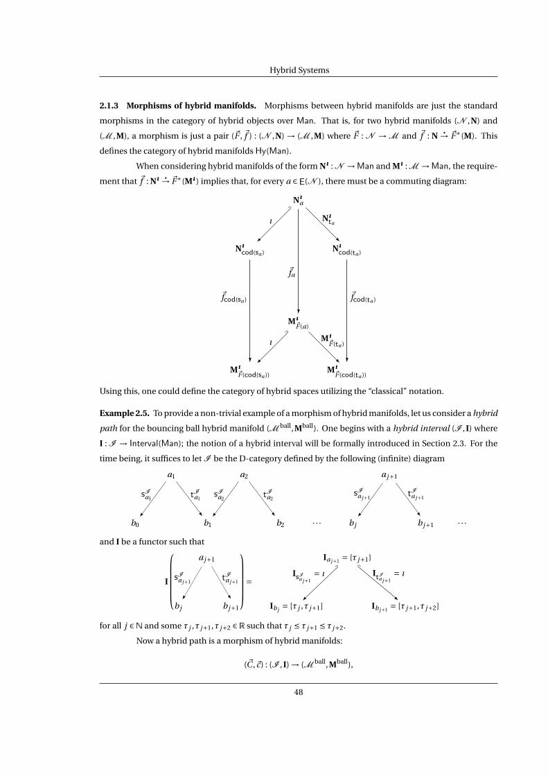
Hybrid Systems
2.1.3 Morphisms of hybrid manifolds. Morphisms between hybrid manifolds are just the standard
morphisms in the category of hybrid objects over Man. That is, for two hybrid manifolds (N ,N) and
(M ,M), a morphism is just a pair (~F , ~f ) : (N ,N) → (M ,M) where ~F : N → M and ~f : N→ ~F∗(M). This
defines the category of hybrid manifolds Hy(Man).
When considering hybrid manifolds of the form Nııı : N →Man and Mııı : M →Man, the require-
ment that ~f : Nııı → ~F∗(Mııı ) implies that, for every a ∈E(N ), there must be a commuting diagram:
Nıııa
Nıııcod(sa )
ı
⊃
Nıııcod(ta )
Nıııta
-
Mııı~F (a)
~fa
?
Mııı~F (cod(sa ))
~fcod(sa )
?
ı
⊃
Mııı~F (cod(ta ))
~fcod(ta )
?
Mııı~F (ta )
-
Using this, one could define the category of hybrid spaces utilizing the “classical” notation.
Example 2.5. To provide a non-trivial example of a morphism of hybrid manifolds, let us consider a hybrid
path for the bouncing ball hybrid manifold (M ball,Mball). One begins with a hybrid interval (I ,I) where
I : I → Interval(Man); the notion of a hybrid interval will be formally introduced in Section 2.3. For the
time being, it suffices to let I be the D-category defined by the following (infinite) diagram
a1 a2 a j+1
b0
sIa1
b1
sIa2
tIa1
-
b2
tIa2
-
· · · b j
sIa j+1
b j+1
tIa j+1
-
· · ·and I be a functor such that
I
a j+1
b j
sIa j+1
b j+1
tIa j+1
-
=
Ia j+1 = τ j+1
Ib j = [τ j ,τ j+1]
IsIaj+1
= ı
⊃
Ib j+1 = [τ j+1,τ j+2]
ItIaj+1
= ı⊂
-
for all j ∈N and some τ j ,τ j+1,τ j+2 ∈R such that τ j ≤ τ j+1 ≤ τ j+2.
Now a hybrid path is a morphism of hybrid manifolds:
(~C ,~c) : (I ,I) → (M ball,Mball),
48

Hybrid Systems
where ~C : I → M ball and ~c : I→ ~C∗(Mball). To better understand such a morphism, note that the condi-
tions on morphisms of D-categories imply that ~C must take the following values on objects: ~C (a j ) ≡ a and
~C (b j ) ≡ b, where in this case a = E(M ball) and b = V(M ball), and the symbol ≡ denotes “identically
equal to.” In addition, it must be orientation preserving, i.e., if s and t are the orientation functions for
M ball, the morphism ~C must take the following values on morphisms: ~C (sIa j
) ≡ sa and ~C (tIa j) ≡ ta . The
morphism ~C can be visualized as follows:
a j+1
I
b j
sIa j+1
b j+1
tIa j+1
-
a?
............................................
M ball
~C
?
b
sa
?
ta
?......
........
........
........
........
........
........
........
........
........................................................................-
The natural transformation ~c can be thought of as a collection of paths (in the “non-hybrid” sense of the
word) on Mballb such that they satisfy certain “discrete” consistency conditions. Specifically, the natural
transformation can be visualized in the following diagram
Ia j+1 = τ j+1
Ib j = [τ j ,τ j+1]
ı
⊃
Ib j+1 = [τ j+1,τ j+2]
ı
⊂
-
Mballa
~ca j
?
Mballb
ı?
∩
Mballta
?
~cb j+1
~cb j
-
where the condition that this diagram commutes is equivalent to requiring that transitions occur when
the guard is reached.
49

Hybrid Systems
2.1.4 The category of dynamical systems. Let M be a manifold and let X : M → T M be a smooth vector
field, i.e., a section of the tangent bundle. Objects of this form are termed dynamical systems. The category
of dynamical systems, Dyn, has as
Objects: Dynamical systems, i.e., pairs (M ,X ), where M is a manifold and X is a vector fieldon that manifold.
Morphisms: Smooth maps of manifolds f : N → M such that the following diagram
T NT f- T M
N
Y6
f- M
X6
(2.3)
commutes; here T f is the pushforward of f .
Remark 2.1. One might be tempted to define a (categorical) hybrid dynamical system as an object over the
category of dynamical systems, i.e., a functor: D : D →Dyn . While this is a hybrid system (in the classical
sense), it is not an especially interesting one.
Definition 2.2. A (categorical) hybrid system is a tuple1
H= (M ,M,X),
where
¦ (M ,M) is a hybrid manifold,
¦ X = Xbb∈V(M ) is a collection of vector fields with Xb : Mb → T Mb a smooth vector field on Mb , i.e.,
(Mb ,Xb) is an object of Dyn for all b ∈V(M ).
Remark 2.2. The categorical definition of a hybrid system nicely parallels the classical definition of a
dynamical system. A dynamical system consists of a pair (M ,X ), where M is a manifold and X is a vector
field on that manifold. Similarly, a hybrid system is a tuple (M ,M,X), where (M ,M) is a hybrid manifold
and X is a collection of vector fields “on” that hybrid manifold.
Proposition 2.2. There is a bijective correspondence:
Classical Hybrid Systems, (Γ,D,G ,R,X )
lCategorical Hybrid Systems, (M ,Mııı ,X).
Proof. Beginning with a classical hybrid system (Γ,D,G ,R,X ), from the hybrid space associated to this
hybrid system,H= (Γ,D,G ,R), we obtain a hybrid manifold (MΓ,M(D,G ,R)). Define the collection of vector
fields on this hybrid manifold by:
XX = Xi i∈Q=V(MΓ).
1We denote both “classical” and “categorical” hybrid systems by the symbol H; the reason for this will soon become transparent.
50

Hybrid Systems
The tuple (MΓ,M(D,G ,R),XX ) is clearly a categorical hybrid system.
Conversely, for a categorical hybrid system (M ,Mııı ,X), from (M ,Mııı ) we obtain a hybrid space:
H(M ,Mııı ) = (ΓM = (QM ,EM ),DMııı ,GMııı ,RMııı ).
Defining
XX = Xbb∈QM=V(M ),
the end result is a classical hybrid system (ΓM ,DMııı ,GMııı ,RMııı ,XX).
Example 2.6. From the bouncing ball hybrid system Hball = (Γball,Dball,Gball,Rball,X ball) introduced in
Example 2.1, we obtain a categorical hybrid system:
(M ball,Mball,Xball),
where (M ball,Mball) is the hybrid manifold associated to the hybrid space of the bouncing ball as intro-
duced in Example 2.3 and Xball = X ball1 . This categorical hybrid system can be visualized graphically using
the original data defining the system Hball as follows2
(M ball,Mball,Xball) =
Gballe
(Dball1 ,X ball
1 )
ı?
∩
Rballe
?
Example 2.7. For the water tank hybrid system Htank = (Γtank,Dtank,G tank,Rtank,X tank) introduced in Ex-
ample 2.2 we obtain a categorical hybrid system:
(M tank,Mtank,Xtank),
where (M tank,Mtank) is the hybrid manifold associated to the hybrid space of the bouncing ball as intro-
duced in Example 2.4, and Xtank = X tankb b∈V(M tank)=Qtank = X tank
1 ,X tank2 . This categorical hybrid system
can be visualized graphically using the original data defining the system Htank as follows
(M tank,Mtank,Xtank) =
G tanke1
(Dtank1 ,X tank
1 )
ı
⊃
(Dtank2 ,X tank
2 )
Rtanke1
-
G tanke2
ı⊂
-
Rtanke2
2Note that this is not a diagram in a category, but rather a convenient way for representing the data defining a categorical hybridsystem.
51

Hybrid Systems
2.1.5 The category of hybrid systems. With the categorical formulation of hybrid systems, we can form
the category of hybrid systems, HySys, with
Objects: Hybrid systems, (M ,M,X),Morphisms: Pairs (~F , ~f ) : (N ,N,Y) → (M ,M,X), where (~F , ~f ) : (N ,N) → (M ,M) is a mor-
phism in Hy(Man) such that there is a commuting diagram:
T NbT ~fb- T M~F (b)
Nb
Yb
6
~fb- M~F (b)
X~F (b)
6
for all b ∈ V(N ). That is, for all b ∈ V(N ), ~fb : (Nb ,Yb) → (M~F (b),X~F (b)) is a morphism inDyn.
Remark 2.3. The definition of the category of hybrid systems again nicely parallels the definition of the
category of dynamical systems. In the latter case, morphisms are morphisms of manifolds such that the
vector fields on each manifold are f -related. Similarly, a morphism of hybrid systems is a morphism of
hybrid manifolds such that the collections of vector fields are “hybrid (~F , ~f )-related.”
2.2 Hybrid Intervals
This section begins with the introduction of the “standard” hybrid interval (much in the spirit
of [68, 69, 82, 83, 118, 119]). We then associate to a hybrid interval its categorical counterpart, i.e., a
categorical hybrid interval. In order to do so, we introduce interval subcategories of some categories of
interest:
Grph, Dcat, Man, Hy(Man). (2.4)
These interval subcategories can be thought of as a generalization of the standard interval (for example,
in R) and, as such, will be instrumental in defining trajectories of hybrid systems. For example, a trajec-
tory of an object in any of the categories given in (2.4) is just a morphism from an object of the interval
subcategory to this object.
2.2.1 Hybrid intervals. Hybrid intervals can be thought of as the “time domain” for trajectories of hy-
brid systems. A hybrid interval is a pair (Λ, I), where
¦ Λ= 0,1,2, . . . ⊆N is a finite or infinite indexing set,
¦ I = Ii i∈Λ where for each i ∈Λ, Ii is defined as follows:
Ii = [τi ,τi+1] if i , i +1 ∈Λ
IN−1 = [τN−1,τN ] or [τN−1,τN ) or [τN−1,∞) if |Λ| = N , N finite.
52

Hybrid Systems
Here, for all i , i +1 ∈Λ, τi ≤ τi+1 with τi ,τi+1 ∈R, and τN−1 ≤ τN with τN−1,τN ∈R.
Remark 2.4. It is sometimes notationally convenient to utilize a set of switching times instead of intervals.
Specifically, we can specify a hybrid interval equivalently as a pair (Λ, τi i∈Λ) such that τi ≤ τi+1. From
this we obtain intervals Ii = [τi ,τi+1] when i , i +1 ∈ Λ. If |Λ| = N is finite, we can specify a final interval
IN−1 as above.
Example 2.8. To provide a simple example, let Λ= 0,1,2. Associated to this indexing set there are three
intervals, e.g.,
I0 = [τ0,τ1], I1 = [τ1,τ2], I2 = [τ2,∞).
Example 2.9. To provide a much more interesting example, let ar nn∈N be a geometric sequence. Then
to this geometric sequence, we have an associated hybrid interval (N, I (a,r)), termed the geometric hybrid
interval, where
I (a,r)i = [τ(a,r)
i ,τ(a,r)i+1 ],
with τ(a,r)0 = 0 and
τ(a,r)i+1 = τ(a,r)
i +ar i =i∑
n=0ar n .
Hybrid intervals of this form, as we will see, naturally arise in Zeno hybrid systems.
We would like to understand hybrid intervals categorically. In order to do so, we will introduce
the notion of an interval subcategory of a category. We first introduce intervals in the category of graphs,
which define intervals in the category of D-categories. Finally, we use intervals in the category of mani-
folds to define hybrid intervals categorically.
2.2.2 Intervals in Grph. For a finite or infinite indexing set Λ= 0,1,2, . . . ⊆N we have an associated a
graph ΓΛ = (QΛ,EΛ), where QΛ =Λ and EΛ is the set of pairs η j+1 = ( j , j +1) such that j , j +1 ∈Λ. Define
Interval(Grph) as the full subcategory of Grph with objects graphs of this form, i.e., graphs obtained from
indexing sets. That is, Interval(Grph) consists of graphs of the form:
0η1 - 1
η2 - 2 · · · jη j+1- j +1 · · · (2.5)
Example 2.10. For the simple indexing set Λ= 0,1,2 , ΓΛ is the graph:
0η1 - 1
η2 - 2.
For an indexing set Λ=N, the graph is of the form given in (2.5).
2.2.3 Intervals in Dcat. Intervals in D-categories are obtained from the intervals in Grph, i.e., using the
isomorphism of categories given in Theorem 1.1, we define:
Interval(Dcat) := dcat(Interval(Grph)).
53
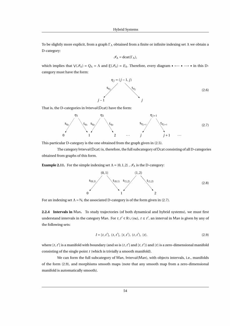
Hybrid Systems
To be slightly more explicit, from a graph ΓΛ obtained from a finite or infinite indexing set Λ we obtain a
D-category:
IΛ = dcat(ΓΛ),
which implies that V(IΛ) = QΛ = Λ and E(IΛ) = EΛ. Therefore, every diagram • ←− • −→ • in this D-
category must have the form:
η j = ( j −1, j )
j −1
sη j
j
tη j
-(2.6)
That is, the D-categories in Interval(Dcat) have the form:
η1 η2 η j+1
0
sη1
1
sη2
tη1
-
2
tη2
-
· · · j
sη j+1
j +1
tη j+1
-
· · ·
(2.7)
This particular D-category is the one obtained from the graph given in (2.5).
The category Interval(Dcat) is, therefore, the full subcategory of Dcat consisting of all D-categories
obtained from graphs of this form.
Example 2.11. For the simple indexing set Λ= 0,1,2 , IΛ is the D-category:
(0,1) (1,2)
0
s(0,1)
1
s(1,2)
t(0,1)
-
2
t(1,2)
-
(2.8)
For an indexing set Λ=N, the associated D-category is of the form given in (2.7).
2.2.4 Intervals in Man. To study trajectories (of both dynamical and hybrid systems), we must first
understand intervals in the category Man. For t , t ′ ∈ R∪ ∞, t ≤ t ′, an interval in Man is given by any of
the following sets:
I = [t , t ′], (t , t ′], [t , t ′), (t , t ′), t . (2.9)
where [t , t ′] is a manifold with boundary (and so is (t , t ′] and [t , t ′)) and t is a zero-dimensional manifold
consisting of the single point t (which is trivially a smooth manifold).
We can form the full subcategory of Man, Interval(Man), with objects intervals, i.e., manifolds
of the form (2.9), and morphisms smooth maps (note that any smooth map from a zero-dimensional
manifold is automatically smooth).
54

Hybrid Systems
Definition 2.3. An interval in Hy(Man) is a pair (I ,I), where
I : I → Interval(Man),
which must satisfy:
¦ I is an object of Interval(Dcat).
¦ For all i ∈V(I ),
Ii = [τi ,τi+1] if i , i +1 ∈V(I )
IN−1 = [τN−1,τN ] or [τN−1,τN ) or [τN−1,∞) if |V(I )| = N , N finite.
¦ For every η ∈E(I ), there is the associated diagram in I :
Iη = Icod(sη) ∩ Icod(tη)
Icod(sη)
Isη = ι
⊃
Icod(tη).
Itη = ι⊂
-
2.2.5 Intervals in Hy(Man). For every η ∈ E(I ), η = (i , i +1) for i , i +1 ∈ V(I ), Definition 2.3 implies
that for every such edge there exist τ,τ′,τ′′ ∈R, with τ≤ τ′ ≤ τ′′, such that
I(i ,i+1) = τ′
Ii = [τ,τ′]
Is(i ,i+1) = ι
⊃
Ii+1 = [τ′,τ′′] or [τ′,τ′′) or [τ′,∞).
It(i ,i+1) = ι
⊂
-
If I is the D-category in (2.7), an example of an interval in Man is given by I : I → Interval(Man) where
I(I ) =
τ1 τ2 τ j+1
[τ0,τ1]
⊃
[τ1,τ2]
⊃⊂
-
[τ2,τ3]
⊂
-
· · · [τ j ,τ j+1]
⊃
[τ j+1,τ j+2]
⊂
-
· · ·
(2.10)
with τ1,τ2, . . . ,τ j+1, . . . the set of switching times.
Let Interval(Hy(Man)) be the full subcategory of Hy(Man) with objects all intervals in Hy(Man).
The importance of intervals in Hy(Man) is that to every hybrid interval (as introduced in Paragraph 2.2.1),
we can associate an object of Interval(Hy(Man)), and vice versa.
Remark 2.5. One can now define paths as in Example 2.5. A hybrid path of a hybrid manifold (M ,M) is an
object (I ,I) of Interval(Hy(Man)) together with a morphism of hybrid manifolds: (~C ,~c) : (I ,I) → (M ,M).
Paths can also be considered in Hy(Top) and other related categories of hybrid objects.
Proposition 2.3. There is a bijective correspondence:
Hybrid Intervals, (Λ, I) ↔ Intervals in Hy(Man), I : I → Interval(Man).
55

Hybrid Systems
Proof. Consider a hybrid interval (Λ, I) with I = Ii i∈Λ. We have the following associations:
Λ 7→ ΓΛ ∈Ob(Interval(Grph)) 7→ IΛ ∈Ob(Interval(Dcat)).
Therefore, to the pair (Λ, I) we have the associated functor and D-category:
II : IΛ → Interval(Man)
where
II
e
sor(e)
se
tar(e)
te
-
:=
IIe := Isor(e) ∩ Itar(e)
IIsor(e) := Isor(e)
ι
⊃
IItar(e) := Itar(e),
ι
⊂
-
for every e ∈E(IΛ) = EΛ.
Conversely, given an object (I ,I) of Interval(Hy(Man)), we have an associated hybrid interval:
(V(I ), II = Ii i∈V(I )).
The definition of intervals in Hy(Man) imply that this is a hybrid interval.
Notation 2.1. As a result of Proposition 2.3, we will refer to objects of Interval(Hy(Man)) as categorical
hybrid intervals or just hybrid intervals.
Example 2.12. For the simple hybrid interval (Λ, I) introduced in Example 2.8, the associated categorical
interval is given by:
II : IΛ → Interval(Man),
where IΛ is the D-category given in (2.8) and II is defined by:
II
(0,1) (1,2)
0
s(0,1)
1
s(1,2)
t(0,1)
-
2
t(1,2)
-
=
II(0,1) = τ1 II
(1,2) = τ2
II0 = [τ0,τ1]
IIs(0,1)
= ı
⊃
II2 = [τ1,τ2]
IIs(1,2)
= ı
⊃IIt(0,1)
= ı⊂
-
II2 = [τ2,∞)
IIt(1,2)
= ı⊂
-
56

Hybrid Systems
Example 2.13. For the geometric hybrid interval (N, I (a,r)) introduced in Example 2.9, the associated cat-
egorical interval is given by:
I(a,r) : IN→ Interval(Man),
where I(a,r) takes the values indicated in the following diagram:
I(a,r)
η1 η2 η j+1
0
sη1
1
sη2
tη1
-
2
tη2
-
· · · j
sη j+1
j +1
tη j+1
-
· · ·
=
I(a,r)η1
= a I(a,r)η2
= a(1+ r)
I(a,r)0 = [0, a]
ı
⊃
I(a,r)1 = [a, a(1+ r)]
ı
⊃
ı
⊂
-
I(a,r)2 = [a(1+ r), a(1+ r + r 2)]
ı
⊂
-
· · ·
I(a,r)η j+1
=
j∑n=0
ar n
I(a,r)j =
[j−1∑n=0
ar n ,j∑
n=0ar n
]ı
⊃
I(a,r)j+1 =
[j∑
n=0ar n ,
j+1∑n=0
ar n
]ı⊂
-
· · ·
2.3 Hybrid Trajectories
This goal of this section is to introduce trajectories of hybrid systems in the context of our cate-
gorical formulation of hybrid system. Utilizing (categorical) hybrid intervals it is a simple matter to define
trajectories of hybrid systems. We define the interval subcategory of Dyn, which is used to construct the
interval subcategory of HySys. A trajectory of a hybrid system is just a morphism from an object in the
interval subcategory of HySys to the hybrid system. We conclude by demonstrating that this formulation
is equivalent to the “standard” notion of an execution.
The constructions presented in this section are motivated by similar ideas that appeared in the
study of bisimulation relations; see [56] and the references therein.
2.3.1 Intervals in Dyn. Trajectories of dynamical systems are morphisms in Dyn whose domain is an
interval in Man together with a vector field that is a “clock”. Specifically, let I be an interval in Man, M a
smooth manifold, and X a vector field on that manifold. Consider a smooth map c : I → M . This map is
said to be a trajectory (or flow or integral curve) of X on M if
c(t ) = X (c(t )) (2.11)
57

Hybrid Systems
for t ∈ I . This is equivalent to requiring that the following diagram
T IT c- T M
I
ddt
6
c - M
X
6
(2.12)
commute. That is, for t ′ ∈ I ,
c(t ′) = Tt ′c
(d
dt
∣∣∣∣t ′
)∈ Tc(t ′)M
So the commutativity of (2.12) enforces condition 2.11, or just c = X (c), which is the usual requirement on
a trajectory.
Therefore, we define the category Interval(Dyn) to be the full subcategory of Dyn consisting of all
objects of the form (I ,d/dt) where I is an object in Interval(Man); here, the vector field d/dt can be thought
of as a unit clock, i.e., the vector field x = 1.
Definition 2.4. A trajectory of a dynamical system (M ,X ) is a morphism in Dyn:
c : (I ,d/dt) → (M ,X ),
where (I ,d/dt) is an object of Interval(Dyn).
Some further explanation of trajectories of dynamical systems is needed because of the specific
domains for these curves that we are considering; that is, I may be a closed interval or a point.
In the case when I = [t0, t1] with t1 > t0, we view I as a manifold with boundary ∂I = t0, t1. We
define c at these endpoints by:
c(t0) := limt→t+0
c(t ), c(t1) := limt→t−1
c(t ).
Similar definitions hold when I = [t0, t1) and I = (t0, t1]. In either of these cases, we again consider the
dynamical system (I ,d/dt), and say that c : I → M is an integral curve of X if c : (I ,d/dt) → (M ,X ) is a
morphism in Dyn, i.e., if (2.12) commutes.
When I = t0 every map c : I = t0 → M is an integral curve of X , and we define c(t0) := X (c(t0)).
There are ways to justify this by (for example, when dimM > 0 and c(t0) is not on the boundary of M)
considering an open interval containing t0. By slight abuse of notation, we still write (t0,d/dt) in this
case; although, it should be understood that what is meant by this is (2.12) trivially commutes, since the
diagram commuting amounts to evaluating X at c(t0).
Example 2.14. For the “dynamical system” portion of the bouncing ball hybrid system as introduced in
Example 2.1, (Dball1 ,X ball
1 ), for an interval [t0, t1] and an initial condition x = (x1, x2)T we obtain a trajectory
for this dynamical system c : ([t0, t1],d/dt) → (Dball1 ,X ball
1 ) given by:
c(t ) = − g (t−t0)2
2 +x2(t − t0)+x1
−g (t − t0)+x2
Clearly, c = X ball
1 (c).
58

Hybrid Systems
GeD1
Re
c0(τ1)
c1(τ2)
c0(τ0) c1(τ1) c2(τ2)
Figure 2.6: A graphical illustration of an execution.
Definition 2.5. An execution of a hybrid system H= (Γ,D,G ,R,X ) is a tuple:
ε= (Λ, I ,ρ,C )
where
¦ (Λ, I) is a hybrid interval.
¦ ρ : Λ→Q is a map such that for all i , i +1 ∈Λ, ei := (ρ(i ),ρ(i +1)) ∈ E . This is the discrete evolution
of the execution.
¦ C = ci i∈Λ is a set of continuous trajectories such that ci : (Ii ,d/dt) → (Dρ(i ),Xρ(i )) for all i ∈ Λ, i.e.,
ci : Ii → Dρ(i ) is a trajectory of Xρ(i ) and thus satisfies ci (t ) = Xρ(i )(ci (t )) for t ∈ Ii .
We require that for all i , i +1 ∈Λ,
(1) ci (τi+1) ∈Gei
(2) Rei (ci (τi+1)) = ci+1(τi+1).
The continuous initial condition of an execution ε is, when I0 = [τ0,τ1], given by c0(τ0) ∈ Dρ(0).
The discrete initial condition is given by ρ(0). Note that given an initial condition, it is by no means
assumed that there is a unique execution with this initial condition. We never concern ourselves with
uniqueness because the results presented never need to make this assumption in order to be valid.
Remark 2.6. In the definition of an execution we did not specify when the switching should occur once the
guard is reached, i.e., we did not specify whether we are considering as-is (forced) or enabling semantics
(see [109] for more on the semantics of hybrid systems). Again, the theorems introduced do not depend
on this choice, so we opted for simplicity by not making a specific choice regarding transition semantics.
In all of the examples, as-is semantics are used.
59

Hybrid Systems
Example 2.15. An graphical illustration of an execution with the same hybrid interval as the one given in
Example 2.8 can be seen in Figure 2.6. In this case, the hybrid system consists of a single domain, guard
and reset map; therefore, the discrete evolution ρ(i ) = 1 for i = 1,2,3. Hybrid systems of this form are
termed simple hybrid systems and will be discussed in detail in Chapter 3.
Example 2.16. The bouncing ball hybrid system allows for the unique luxury of explicitly solving for its
executions. That is, given an initial condition, we can explicitly produce a corresponding execution.
Starting at the initial condition x = (x1, x2)T ∈ Dball1 at time τ0, the system evolves according to
the dynamics X ball1 ,
c0(t ) = − g (t−τ0)2
2 +x2(t −τ0)+x1
−g (t −τ0)+x2
until the guard Gball
e is reached, which occurs in time and space at:
τ1 = τ0 +x2 +
√2g x1 +x2
2
g
c0(τ1) = 0
−√
2g x1 +x22
Applying the reset map Rball
e to c0(τ1) yields the initial condition to subsequent trajectory c1(t ) on Dball1
which starts at time τ1, i.e.,
c1(t ) = − g (t−τ1)2
2 + r(t −τ1)√
2g x1 +x22
−g (t −τ1)+ r√
2g x1 +x22
wherein we can again determine the subsequent time and point in which the guard is reached:
τ2 = τ1 +2r
√2g x1 +x2
2
g
c0(τ1) = 0
−r√
2g x1 +x22
Repeating this process iteratively yields an execution:
ε= (Λ, I ,ρ,C ).
Here Λ=N, I = Ii i∈N where Ii = [τi ,τi+1] with
τ1 = τ0 +x2 +
√2g x1 +x2
2
g,
τi+1 = τi +2r i
√2g x1 +x2
2
g, i ≥ 1.
Since there is only one domain, ρ(i ) ≡ 1. Finally, C = ci i∈N with
ci (t ) = − g (t−τi )2
2 + r i (t −τi )√
2g x1 +x22
−g (t −τi )+ r i√
2g x1 +x22
.
60

Hybrid Systems
xx_dot
-10
-5
0
5
0 2 4 6 8 10 12 14 16 18 20
Displacement
Figure 2.7: Positions and velocities over time of an execution of the bouncing ball hybrid system.
An execution of the bouncing ball can be seen in Figure 2.7.
2.3.2 Zeno executions. A particular class of executions of hybrid systems that will be of particular in-
terest are Zeno executions.
Definition 2.6. An execution ε= (Λ, I ,ρ,C ) of H is Zeno if Λ=N and
∞∑i=0
(τi+1 −τi ) = limi→∞
τi = τ∞
for some finite constant τ∞, termed the Zeno time.
Example 2.17. Using the constructed executions for the bouncing ball hybrid system, we can verify that
it is Zeno. That is,
∞∑i=0
(τi+1 −τi ) =x2 + (1−2g )
√2g x1 +x2
2
g+
∞∑i=0
2
√2g x1 +x2
2
gr i
where the series on the right is a geometric series, and converges if 0 ≤ r < 1. What this says physically is
if the ball looses energy on each bounce, then it will eventually stop bouncing; moreover, it will do so in
finite time. We give conditions (in Chapter 5) on the Zenoness of the bouncing ball without solving for the
vector fields.
Consider again the geometric hybrid interval, (N, I (a,r)). It is easy to see that
∞∑i=0
(τ(a,r)i+1 −τ(a,r)
i ) =∞∑
i=0ar i .
Now, picking initial conditions x1 = a2g /8 and x2 = 0 for an execution of the bouncing ball yields
∞∑i=0
(τi+1 −τi ) =±(
1
2a(1−2g )+
∞∑i=0
ar i
),
where the expression on the right is positive if a is positive and negative if a is negative. Therefore, the
hybrid interval for the bouncing ball is an example of a geometric hybrid interval.
61

Hybrid Systems
2.3.3 Intervals in HySys. The interval category of HySys, denoted by Interval(HySys), is the full subcat-
egory of HySys with objects consisting of hybrid systems of the form:
(I ,I,d///dt),
where
¦ (I ,I) is a hybrid interval, i.e., an object of Interval(Hy(Man)),
¦ d///dt j = d/dt for all j ∈Ob(I ).
For example, if (I ,I) is the hybrid interval given in (2.10), the corresponding object (I ,I,d///dt)
of Interval(HySys) can be visualized graphically as follows:
τ1 τ2 τ j+1
([τ0,τ1],d/dt)
⊃
([τ1,τ2],d/dt)
⊃⊂
-
([τ2,τ3],d/dt)
⊂
-
· · · ([τ j ,τ j+1],d/dt)
⊃
([τ j+1,τ j+2],d/dt)
⊂
-
· · ·One of the many benefits of defining intervals in HySys is the way in which they allow us to
parallel the definition of trajectories of dynamical systems as given in Definition 2.4.
Definition 2.7. A trajectory of a hybrid system (M ,M,X) is a morphism in HySys:
(~C ,~c) : (I ,I,d///dt) → (M ,M,X),
where (I ,I,d///dt) is an object of Interval(HySys).
Note that the functor ~C corresponds to the “discrete” portion of the trajectory, while the natural
transformation ~c corresponds to the “continuous” portion. In particular, it follows that
~c j (t ) = X~C ( j )(~c j (t ))
for every object j ∈V(I ).
The discrete initial condition is given by ~C (0) and the continuous initial condition is given by
~c0(τ0) ∈ M~C (0) with τ0 the right endpoint of I0, i.e., the initial condition to the trajectory is (~C (0),~c0(τ0)).
Proposition 2.4. There is a bijective correspondence:
Executions of H ↔ Trajectories of (M ,Mııı ,X).
Proof. If ε= (Λ, I ,ρ,C ) is an execution of H= (Γ,D,G ,R,X ), to the pair (Λ, I) we have an associated object
of Interval(Hy(Man)):
II : IΛ → Interval(Man).
From this, we obtain an object of Interval(HySys):
(IΛ,II ,d///dt).
62

Hybrid Systems
The remaining data defining the execution ε= (Λ, I ,ρ,C ), i.e., the discrete evolution ρ and the continuous
evolution C , allows us to define a morphism:
(~Cρ,~cC ) : (IΛ,II ,d///dt) → (MΓ,M(D,G ,R),XX ),
where (MΓ,M(D,G ,R),XX ) is the categorical hybrid system obtained from the classical hybrid system H via
Proposition 2.2. The morphism of D-categories ~Cρ : IΛ →MΓ is defined on objects of IΛ by
~Cρ(a) = e j = (ρ( j ),ρ( j +1)) if a = ( j , j +1) ∈E(IΛ)
ρ( j ) if a = j ∈V(IΛ)
and on morphisms in the obvious way:
~Cρ(sIΛa ) := sMΓ
~Cρ(a), ~Cρ(tIΛ
a ) := tMΓ
~Cρ(a),
with (sIΛ ,tIΛ ) the orientation for IΛ and (sMΓ ,tMΓ ) the orientation for MΓ. It follows that this is a valid
morphism of D-categories. Finally, define the natural transformation
~cC : II → ~C∗ρ (M(D,G ,R))
on objects of IΛ as follows:
(~cC )a = c j |I j ∩I j+1 if a = ( j , j +1) ∈E(IΛ)
c j if a = j ∈V(IΛ).
To verify that this is a natural transformation, we need only verify that the following diagram
IIj = I j
⊃ II( j , j+1) = I j ∩ I j+1 ⊂ - II
j+1 = I j+1
M(D,G ,R)~Cρ( j )
= Dρ( j )
(~cC ) j = c j
?ı ⊃ M(D,G ,R)
~Cρ( j , j+1)=Ge j
(~cC )( j , j+1) = c j |I j ∩I j+1
? M(D,G ,R)
~Cρ(sIΛ( j , j+1))
= Re j
- M(D,G ,R)~Cρ( j+1)
= Dρ( j+1)
(~cC ) j+1 = c j+1
?
commutes for every ( j , j +1) ∈E(I ). But this happens exactly when, for I j = [τ j ,τ j+1],
c j (τ j+1) ∈Ge j , c j+1(τ j+1) = Re j (c j (τ j+1)),
which are just requirements (1) and (2) given in Definition 2.5.
The converse direction proceeds in much the same manner, so we will be brief. Let (M ,Mııı ,X)
be a categorical hybrid system for which we have an associated hybrid system (ΓM ,DMııı ,GMııı ,RMııı ,XX)
as given in Proposition 2.2. For a trajectory (~C ,~c) : (I ,I,d///dt) → (M ,Mııı ,X), we define a corresponding
execution as
(V(I ), II, ~C |V(I ), ~c j j∈V(I )),
where (V(I ), II) is the hybrid interval obtained from I : I → Interval(Man) via Proposition 2.3 and ~C |V(I )
is the object function of the functor ~C restricted to the elements of V(I ). It is easy to verify that this is a
valid execution.
63

Hybrid Systems
Example 2.18. Consider the categorical bouncing ball hybrid system (M ball,Mball,Xball) and a trajectory
(~C ,~c) : (I ,I,d///dt) → (M ball,Mball,Xball),
which, for example, can be obtained from the executions of Hball introduced in Example 2.16. The con-
dition that this is a trajectory implies that (~C ,~c) : (I ,I) → (M ball,Mball) in Hy(Man) is a hybrid path as
discussed in Example 2.5. The additional condition, and the one that makes (~C ,~c) a trajectory, is that the
collection of paths defined by ~c satisfy the ordinary differential equation Xballb .
Another of the many benefits obtained from defining trajectories of hybrid systems categorically
is that morphisms of hybrid systems carry trajectories of one hybrid system to trajectories of another
hybrid system.
Lemma 2.1. If (~F , ~f ) : (N ,N,Y) → (M ,M,X) is a morphism of hybrid systems, and (~C ,~c) : (I ,I,d///dt) →(N ,N,Y) is a trajectory of (N ,N,Y), then
(~F , ~f ) (~C ,~c) : (I ,I,d///dt) → (M ,M,X)
is a trajectory of (M ,M,X).
The proof of this statement is immediately obvious using the categorical framework for hybrid
systems, while it is not immediately clear if one were to consider the standard notion of an execution.
64

Part II
Hybrid Systems
65

Chapter 3
Simple Hybrid Reduction & Bipedal
Robotic Walking
Hybrid systems introduce a level of complexity not found in their continuous and discrete coun-
terparts, e.g., simulating hybrid systems is orders of magnitude more difficult than simulating their con-
tinuous counterparts due to the presence of state dependent events. This added complexity makes the
dimensionality of hybrid systems a critical factor in understanding, analyzing, verifying and control-
ling these systems and motivates the importance of understanding geometric reduction in a hybrid set-
ting. Since it is not possible to directly apply classical (continuous) reduction to hybrid systems—the
nonsmooth nature of these systems inherently violates the assumptions needed to perform this type of
reduction—we would like to answer the question:
If it is possible to reduce the continuous components of a hybrid system, when is it possible toreduce the entire hybrid system?
This chapter addresses this question in the context of mechanical systems undergoing impacts;
we will address this question for general hybrid system in Chapter 4. The simple structure of mechan-
ical systems undergoing impacts allows us to derive explicit conditions on when continuous reduction
can be applied to the continuous component of these systems so as to be consistent with the discrete
component, i.e., when hybrid reduction can be performed.
History. Lagrangians and Hamiltonians provide the basic elements for describing the behavior of physical
systems. For mechanical systems, one begins with a configuration space Q and a Lagrangian L : TQ → R
or a Hamiltonian H : T ∗Q →R given in coordinates by1
L(q, q) = 1
2qT M(q)q −V (q), H(q, p) = 1
2pT M(q)−1p +V (q).
1We slightly abuse notation here by using “matrix” notation; this is done only in the introduction because of its (presumed)familiarity.
66

Simple Hybrid Reduction & Bipedal Robotic Walking
It is possible to reduce the dimensionality of systems of this form when they have symmetries through
reduction; this process plays a fundamental role in understanding the many important and interesting
properties of these systems.
The first form of reduction was discovered by Routh in 1860 [100] (see [87] for a more mod-
ern account)—now understood to be an abelian form of Lagrangian reduction—which is concerned with
cyclic Lagrangians, i.e., Lagrangians that are independent of certain “cyclic” variables. The symmetries
of these systems are generated by these cyclic variables. Given a cyclic Lagrangian, the phase space of
the system (the tangent bundle of the configuration space) can be reduced, flows of the original system
can be projected down to flows of the reduced system, and flows of the reduced system can be used to
reconstruct flows of the full-order system.
Lagrangian reduction provides the first step toward a more general type of reduction: Hamil-
tonian (or symplectic) reduction. This form of reduction begins with a Lie group together with an action
of this Lie group on the phase space (a symplectic manifold); this makes explicit the symmetries of the
system. One then looks for a momentum map from the phase space to the dual of the Lie algebra of
the Lie group; this makes explicit the conserved quantities of the system. The combination of this data
defines a Hamiltonian G-space, which provides the ingredients necessary for classical Hamiltonian reduc-
tion. The classical reduction theorem, first established by Marsden and Weinstein [88], says that when the
Hamiltonian G-space satisfies certain conditions, the phase space can be reduced to a new space which is
also a symplectic manifold, with a symplectic structure induced from the one on the phase space. More-
over, given a G-invariant Hamiltonian on the phase space, the corresponding trajectories of the associated
Hamiltonian vector field reduce to trajectories on the reduced phase space.
Simple hybrid reduction. In this chapter, we begin by considering a class of mechanical systems with
unilateral constraints (usually physical in nature) on the configuration space, i.e., there is a function h :
Q →R describing the admissible configurations of the system: Q|h(q)≥0. When considering Lagrangians,
a unilateral constraint function defines a hybrid Lagrangian, which is a tuple L = (Q,L, h). In the case
of Hamiltonians, simple hybrid mechanical systems (HMS’s), H = (Q,H , h), are considered. In both cases,
the term “hybrid” is used because the constraints on the configuration space result in discontinuities in
the vector field describing the evolution of the mechanical system. Therefore, we can explicitly associate
hybrid systems, HL and HH, to hybrid Lagrangians and HMS’s, respectively. We provide conditions on
when it is possible to reduce hybrid systems of this form, along with more general simple hybrid systems
(hybrid systems consisting of one domain and one edge) whose dynamics are dictated by a Hamiltonian
system.
A cyclic hybrid Lagrangian is a hybrid Lagrangian in which L is cyclic (coupled with the cyclicity
of the unilateral constraint function h); we demonstrate explicitly how a Lagrangian hybrid system, HL,
can be obtained from a hybrid Lagrangian, L, with dynamics dictated by the Euler-Lagrange equations
of a Lagrangian. From a cyclic hybrid Lagrangian we obtain a hybrid Routhian Lµ = (Qµ,Lµ, hµ), which
is also a hybrid Lagrangian, and so has an associated hybrid system, HLµ , with dynamics dictated by the
67

Simple Hybrid Reduction & Bipedal Robotic Walking
Routhian. We prove that hybrid flows (or executions) of HL project to hybrid flows of HLµ , and that hybrid
flows of HL can be reconstructed from hybrid flows of HLµ . These results motivate the consideration of a
more general form of hybrid reduction: hybrid Hamiltonian (or symplectic) reduction.
In order to perform Hamiltonian reduction, we begin by considering a Hamiltonian G-space
and give conditions on the elements of this G-space so that it defines a hybrid Hamiltonian G-space.
Explicitly, this involves defining the notion of a hybrid group action and a hybrid momentum map, which
is first done in the general setting of simple hybrid systems, followed by the special case of HMS’s. Using
these general notions, conditions are obtained on when a simple hybrid system, H, can be reduced; the
result is a simple hybrid system Hµ.
Bipedal Walking. A very interesting and promising application of hybrid reduction is bipedal robotic
walking since bipedal walkers are naturally modeled by hybrid systems—the continuous component con-
sists of the dynamics dictated by the Lagrangian modeling this system, and the discrete component con-
sists of the impact equations which instantaneously change the velocity of the system when the foot con-
tacts the ground. In order to apply reduction to systems of this form in a useful manner, we introduce
a variation of classical Routhian reduction, functional Routhian reduction, which can be extended to a
hybrid setting in a manner analogous to the extension of classical Routhian reduction.
In classical geometric reduction the conserved quantities used to reduce and reconstruct sys-
tems are constants; this indicates that the “cyclic” variables eliminated when passing to the reduced phase
space are typically uncontrolled. Yet it is often the case that these variables are the ones of interest—it may
be desirable to control the cyclic variables while not affecting the reduced order system. This motivates
an extension of Routhian reduction to the case when the conserved quantities are functions of the cyclic
variables instead of constants.
These concepts motivate our main goal:
Develop a feedback control law that results in walking gaits on flat ground for a three-dimensionalbipedal robotic walker given walking gaits for a two-dimensional bipedal robotic walker.
In order to achieve this goal, we begin by considering Lagrangians that are cyclic except for an
additional non-cyclic term in the potential energy, i.e., almost-cyclic Lagrangians. When Routhian reduc-
tion is performed with a function (of the cyclic variables) the result is a Lagrangian on the reduced phase-
space: the functional Routhian. We are able to show that the dynamics of an almost-cyclic Lagrangian
satisfying certain initial conditions project to dynamics of the corresponding functional Routhian, and
dynamics of the functional Routhian can be used to reconstruct dynamics of the full-order system. In
order to use this result to develop control strategies for bipedal walkers, it first must be generalized to a
hybrid setting. That is, after discussing how to explicitly obtain a hybrid system model of a bipedal walker,
we generalize functional Routhian reduction to a hybrid setting, demonstrating that hybrid flows of the
reduced and full order system are related in a way analogous to the continuous result.
We then proceed to consider two-dimensional (2D) bipedal walkers. It is well-known that 2D
bipedal walkers can walk down shallow slopes without actuation (cf. [90], [54]). [107] used this observa-
68

Simple Hybrid Reduction & Bipedal Robotic Walking
tion to develop a positional feedback control strategy that allows for walking on flat ground. We use these
results to obtain a hybrid system, Hs2D, modeling a 2D bipedal robot that walks on flat ground.
We conclude by considering three-dimensional (3D) bipedal walkers. Our main result is a po-
sitional feedback control law that produces walking gaits in three-dimensions. To obtain this controller
we shape the potential energy of the Lagrangian describing the dynamics of the 3D bipedal walker so that
it becomes an almost-cyclic Lagrangian, where the cyclic variable is the roll (the unstable component) of
the walker. We are able to control the roll through our choice of a non-cyclic term in the potential energy.
Since the functional Routhian hybrid system obtained by reducing this system is Hs2D, by picking the “cor-
rect” function of the roll, we can force the roll to go to zero for certain initial conditions. That is, we obtain
a non-trivial set of initial conditions that provably result in three-dimensional walking.
Related work. The simple hybrid mechanical systems considered have been well-studied in the literature
under many names and incarnations (cf. [36] and the more than 1000 references therein). Amazingly, the
authors are unaware of any results regarding the reduction of systems of this form. General hybrid systems
have been studied extensively; especially relevant are [38] which studies hybrid mechanical systems of
a more general form than considered here, and [66] which considers hybrid systems with symmetries.
Again, the authors are unaware of any results regarding the reduction of these systems; although, the
“non-geometric” reduction of these systems in the context of abstraction and bisimulation relations [96]
has been well-studied and proven useful for verification techniques such as reachability analysis [57].
Classical reduction has developed into a mature area of study over the last forty years (see [89]
for a nice overview of the history of the subject). We will assume that the reader is at least tentatively
familiar with classical reduction, although we briefly review crucial prerequisite material. We refer the
reader to [4, 79, 86, 87, 88] for any necessary background material not covered. Although never explicitly
mentioned, the literature on classical reduction has touched upon issues relating to hybrid reduction.
In [86] a form of discrete reduction is discussed where the assumptions needed to perform this form of
reduction are very similar to conditions enumerated later. Similarly, the reduction of continuous systems
with constraints has been studied in [85] and related references therein. Therefore, the results proven
can be viewed as the next logical step in understanding how to reduce the dimensionality of systems with
symmetry.
The results presented in this chapter have appeared, or will appear, in the following papers:
[8, 15, 17].
3.1 Simple Hybrid Lagrangians & Simple Hybrid Mechanical Systems
In this section, we introduce the notion of simple hybrid Lagrangians and simple hybrid me-
chanical systems. While introducing these definitions, we simultaneously review their continuous “non-
hybrid” counterparts. This is done both to introduce the reader to the notation and simultaneously to
make explicit the natural way that these “hybrid objects” relate to fundamental objects in classical me-
69
Simple Hybrid Reduction & Bipedal Robotic Walking
chanics. This relationship is further explored by introducing examples.
3.1.a Simple Hybrid Lagrangians
We begin by considering simple hybrid Lagrangians.
3.1.1 Lagrangians. Let Q be the configuration space, assumed to be a smooth manifold, and TQ the
tangent bundle of Q (the velocity phase space). Suppose L : TQ → R is a hyperregular Lagrangian (cf.
[4, 87]). In this case, there is a Lagrangian vector field XL on TQ, XL : TQ → T (TQ), associated to L; that
is, there is a dynamical system (TQ,XL) associated to the Lagrangian. For t ∈ [t0, t1], we say that c(t ) =(q(t ), q(t )) is an integral curve of XL with initial condition c(t0) = x0 if
c : ([t0, t1],d/dt) → (TQ,XL)
is a morphism in Dyn, i.e., if
c(t ) = XL(c(t )).
This is equivalent to the curve q(t ) satisfying the classical Euler-Lagrange equations:
d
dt
∂L
∂q(q(t ), q(t ))− ∂L
∂q(q(t ), q(t )) = 0. (3.1)
We will consider primarily Lagrangians describing mechanical, or robotic, systems; that is, La-
grangians given in coordinates by
L(q, q) = 1
2qT M(q)q −V (q), (3.2)
where M(q) is the inertial matrix, 12 qT M(q)q is the kinetic energy and V (q) is the potential energy. In this
case, the Euler-Lagrange equations yield the equations of motion for the system:
M(q)q +C (q, q)q +N(q) = 0, (3.3)
where C (q, q) is the Coriolis matrix (cf. [93]) and N(q) = ∂V∂q (q). Setting x = (q, q), the Lagrangian vector
field, XL, associated to L takes the familiar form.
x = XL(x) = (q,M(q)−1(−C (q, q)q −N(q))
). (3.4)
This process of associating a dynamical system to a Lagrangian will be mirrored in the setting of hybrid
systems. First, we introduce the notion of a hybrid Lagrangian.
Remark 3.1. It is common for other authors to write x as a single vector, i.e., x = (qT , qT )T , rather than a
pair of vectors; we opt for the latter notation in order to avoid the proliferation of transposes. Also, our
notation is supported by the fact that an element of TQ is typically denoted by a pair (q, q) with q ∈Q and
q ∈ TqQ.
70
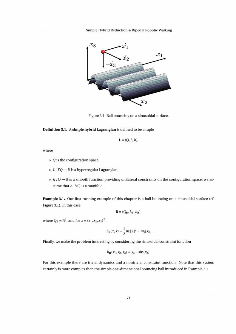
Simple Hybrid Reduction & Bipedal Robotic Walking
Figure 3.1: Ball bouncing on a sinusoidal surface.
Definition 3.1. A simple hybrid Lagrangian is defined to be a tuple
L = (Q,L, h),
where
¦ Q is the configuration space,
¦ L : TQ →R is a hyperregular Lagrangian,
¦ h : Q → R is a smooth function providing unilateral constraints on the configuration space; we as-
sume that h−1(0) is a manifold.
Example 3.1. Our first running example of this chapter is a ball bouncing on a sinusoidal surface (cf.
Figure 3.1). In this case
B = (QB,LB, hB),
where QB =R3, and for x = (x1, x2, x3)T ,
LB(x, x) = 1
2m‖x‖2 −mg x3.
Finally, we make the problem interesting by considering the sinusoidal constraint function
hB(x1, x2, x3) = x3 − sin(x2).
For this example there are trivial dynamics and a nontrivial constraint function. Note that this system
certainly is more complex then the simple one-dimensional bouncing ball introduced in Example 2.1
71

Simple Hybrid Reduction & Bipedal Robotic Walking
yy
xx
xx
zzθθ
Figure 3.2: Pendulum on a cart.
Example 3.2. Our second running example is a constrained pendulum on a cart (cf. Figure 3.2); this is a
variation on the classical pendulum on a cart, where the pendulum is not allowed to “pass through” the
cart, i.e., the cart gives physical constraints on the configuration space. In this case
C = (QC,LC, hC),
where QC =S1 ×R, q = (θ, x)T , and
LC(θ, θ, x, x) = 1
2
(θ x
) mR2 mR cos(θ)
mR cos(θ) M +m
θ
x
−mg R cos(θ).
Finally, the constraint that the pendulum in not allowed to pass through the cart is manifested in the
constraint function
hC(θ, x) = cos(θ).
3.1.b Simple Hybrid Mechanical Systems
We now turn our attention toward Hamiltonians and their hybrid analogues.
3.1.2 Hamiltonians. The starting point for simple mechanical systems is a configuration space Q. Let
T ?Q be the cotangent bundle of Q (the momentum phase space). We denote the pairing between the
vector spaces2 T ?q Q and TqQ by
⟨ · , · ⟩ : T ?q Q ×TqQ →R,
which for (p, v) ∈ T ?q Q ×TqQ is given in coordinates by ⟨p, v⟩ :=∑n
i=1 pi v i , with n = dim(Q).
2We later will use the same notation to denote the pairing between a Lie algebra and its dual.
72

Simple Hybrid Reduction & Bipedal Robotic Walking
Let M(q) be the inertial matrix for a mechanical system and K (q) = M(q)−1. For each q ∈Q, we
consider the K (q)-inner product on the vector space T ?q Q given in coordinates by3
⟨⟨p, p′⟩⟩q = pT K (q)p′ :=n∑
i , j=1pi p′
j Ki j (q)
for p, p′ ∈ T ?q Q; we use || · ||q to denote the corresponding norm on T ?
q Q. This induces (or is obtained from,
depending on the perspective taken) an inner product on TqQ (the M(q)-inner product, which defines a
Riemannian metric on Q) via the Legendre transformation: FL : TQ → T ?Q, where FL(q, q) = (q,M(q)q).
A Hamiltonian is a map H : T ?Q →R. We suppose that the Hamiltonian H describes a mechan-
ical system, i.e., that it has the following form
H(q, p) = 1
2||p||2q +V (q), (3.5)
where 12 ||p||2q is the kinetic energy and V (q) is the potential energy. Note that this Hamiltonian is obtained
from a Lagrangian of the form given in (3.2) via the Legendre transformation.
The cotangent bundle, T ?Q, is a symplectic manifold with its symplectic structure obtained
from the canonical symplectic form given in coordinates by:
ωcanonical =n∑
i=1dq i ∧dpi .
With this symplectic form, we obtain a vector field on T ?Q from a Hamiltonian, XH : T ?Q → T (T ?Q), by
requiring that it satisfies:
d(H) = ιXHωcanonical.
In coordinates, this yields the classical Hamiltonian equations
(q, p) = XH (q, p) =(∂H
∂p(q, p),−∂H
∂q(q, p)
). (3.6)
We refer the reader to [4, 27] and [87] for more details.
Definition 3.2. A simple hybrid mechanical system (HMS) is defined to be a tuple:
H = (Q,H , h),
where H is defined as in (3.5), and h : Q →R is a smooth function that defines constraints on the configu-
ration of the system; again, h−1(0) is assumed to be a manifold.
Utilizing the Legendre transformation, to a hybrid Lagrangian we obtain an associated hybrid
mechanical system. That is, the classical relationship between Lagrangians and Hamiltonians can be
extended to the hybrid setting considered here. This relationship implies that in considering hybrid La-
grangians, one automatically is considering hybrid mechanical systems and vice versa (since we are as-
suming that L is a hyperregular Lagrangian). Therefore, our later results on hybrid Hamiltonian reduction
73

Simple Hybrid Reduction & Bipedal Robotic Walking
x
y
z
Figure 3.3: Spherical pendulum mounted on the floor.
(which are more general then the earlier results on hybrid Lagrangian reduction) are automatically ap-
plicable to hybrid Lagrangians.
Example 3.3. The running example of a HMS will be a spherical pendulum mounted on the floor (Figure
3.3). Here QP = S2 and, using the standard spherical coordinates, we denote an element q ∈ S2 by q =(θ,ϕ)T and we denote an element p ∈ T ?
q S2 by p = (pθ, pϕ)T . For this example, the Hamiltonian HP is
given by
HP(q, p) = 1
2mR2
(p2θ +
p2ϕ
sin2(θ)
)−mg R cos(θ).
Finally, hP is the height function hP(θ,ϕ) = cos(θ), i.e., we have a simple hybrid mechanical system given
by P = (QP,HP, hP).
3.2 Simple Hybrid Systems
In this section, we introduce simple hybrid systems, and show explicitly how to associate to hy-
brid Lagrangians and HMS’s simple hybrid systems. This association is achieved through the use of New-
tonian impact equations, which provide a method for describing the behavior of a mechanical system
undergoing impacts. It is important to note that this construction has support in the literature (cf. [36],
[38], [49]), and hybrid systems of this form have the ability to model a large class of physical systems.
Definition 3.3. A simple hybrid system4 is a tuple:
H= (D,S,R,X ),
3We use the notation “pT K (q)p′” so as to relate “matrix” notation (which is more common when discussing Lagrangians) withsummation notation (which is more common when discussing Hamiltonians and reduction in general). Typically, We will only use“matrix notation” when discussing Lagrangians.
4So named because of its connection with simple HMS’s, coupled with its “simple” structure.
74

Simple Hybrid Reduction & Bipedal Robotic Walking
where
¦ D is a smooth manifold called the domain,
¦ S is an embedded submanifold of D called the switching surface or guard,
¦ R : S → D is a smooth map called the reset map,
¦ X is a vector field on D.
In this case, the hybrid manifold associated to this hybrid system is a tuple DH = (D,S,R) with elements as
defined above. That is, since the graph Γ for a simple hybrid system consists of a single edge and vertex,
i.e., it is of the form:
the associated D-category DΓ is given by:
a
b
sa
?
ta
?
and DH is a functor DH : DΓ →Man defined by:
DH
a
b
sa
?
ta
?
=
S
D
ı
?
R
?
where ı is the natural inclusion.
Remark 3.2. Note that simple hybrid systems are clearly just a special case of the notion of a hybrid system
introduced in Definition 2.1, although we have opted to shift notation slightly. The first noticeable differ-
ence is that there is no reference to an indexing graph Γ. This is because simple hybrid systems always
have as an indexing graph a graph with a single edge and vertex. This also explains why we do not index
the domains, guards, reset maps and vector fields—there is only one of each. Finally, for simple hybrid
systems, we denote the guard by “S” instead of “G”. The motivation for this is that we will use the symbol
“G” to denote groups in this chapter.
Executions for simple hybrid systems are of a somewhat simpler form than the executions for
general hybrid systems as introduced in Definition 2.5. That is, since there is only one domain, the discrete
evolution ρ : Λ → Q must take a single value, and so need not be mentioned. To make this explicit, we
restate the definition of an execution in the context of simple hybrid systems. Moreover, to highlight the
difference between executions of hybrid systems and executions of simple hybrid systems, we refer to the
later as hybrid flows.
75
Simple Hybrid Reduction & Bipedal Robotic Walking
3.2.1 Hybrid flows. A hybrid flow is a tuple:
εH = (Λ, I ,C ),
where
¦ Λ= 0,1,2, . . . ⊆N is a finite or infinite indexing set.
¦ I = Ii i∈Λ is a collection of intervals where Ii = [τi ,τi+1] if i , i + 1 ∈ Λ and IN−1 = [τN−1,τN ] or
[τN−1,τN ) or [τN−1,∞) if |Λ| = N , N finite; here τi ,τi+1,τN ∈R and τi ≤ τi+1,
¦ C = ci i∈Λ is a collection of integral curves of X , i.e., ci (t ) = X (ci (t )) for all i ∈Λ.
In addition, we require that the following conditions hold for every i , i +1 ∈Λ,
(i) ci (τi+1) ∈ S,
(ii) R(ci (τi+1)) = ci+1(τi+1).
The initial condition for the execution is x0 = c0(τ0). When we wish to make explicit the initial condition
of εH we write εH(x0).
Example 3.4. A graphical illustration of a hybrid flow can be seen Figure 2.6. The reader should make the
appropriate changes of notion in this figure as discussed in Remark 3.2.
3.2.a Lagrangian Hybrid Systems
We now discuss how to obtain simple hybrid systems from simple hybrid Lagrangians.
3.2.2 Domains from constraints. Given a smooth (constraint) function h : Q → R on a configuration
space Q such that h−1(0) is a smooth manifold, i.e., 0 is a regular value of h, we can construct a domain
and a guard explicitly. To this constraint function we have an associated domain, Dh , defined to be the
manifold (with boundary):
Dh = (q, q) ∈ TQ : h(q) ≥ 0.
Similarly, we have an associated guard, Sh , defined as the following submanifold of Dh :
Sh = (q, q) ∈ TQ : h(q) = 0 and dhq q ≤ 0,
where in coordinates
dhq =(
∂h∂q1
(q) · · · ∂h∂qn
(q))
.
These constructions will be utilized throughout this chapter.
Definition 3.4. A hybrid system is said to be a Lagrangian hybrid system with respect to a hybrid La-
grangian L = (Q,L, h) if it is of the form:
H= (Dh ,Sh ,R,XL),
where Dh and Sh are the domain and guard associated to h and XL is the vector field associated to L.
76

Simple Hybrid Reduction & Bipedal Robotic Walking
3.2.3 Special Lagrangian hybrid systems. There is a class of Lagrangian hybrid systems that are of
special interest; these model unilaterally constrained systems undergoing impacts [36], and so have reset
maps obtained from Newtonian impact equations.
Given a hybrid Lagrangian L = (Q,L, h), the Lagrangian hybrid system associated to L is the hy-
brid system
HL = (DL,SL,RL,XL),
where DL = Dh , SL =Gh , XL = XL and
RL(q, q) = (q,PL(q, q)),
with PL given in coordinates by:
PL(q, q) = q − (1+ e)dhq q
dhq M(q)−1dhTq
M(q)−1dhTq , (3.7)
where 0 ≤ e ≤ 1 is the coefficient of restitution, e.g., for a perfectly elastic impact e = 1, and for a perfectly
plastic impact e = 0.
Of course, the Lagrangian hybrid system associated to a hybrid Lagrangian is a Lagrangian hy-
brid system w.r.t. this hybrid Lagrangian. The converse statement is not true. General Lagrangian hybrid
systems, as introduced in Definition 3.4, describe a much larger class of systems, e.g., it is not assumed
that the reset map is continuous in the configuration variables. An important class of systems that gen-
eral Lagrangian hybrid systems describe are bipedal robotic walkers (cf. [55, 107, 116]). In fact, general
Lagrangian hybrid systems and the hybrid reduction thereof are used in Section 3.5 to reduce the dimen-
sionality of bipedal walkers. It is then possible to use results relating to two-dimensional bipedal walkers
to allow three-dimensional bipedal walkers to walk while stabilizing to the upright position.
Example 3.5. The Lagrangian hybrid system for the bouncing ball on a sinusoidal surface is given by
HB = (DB,SB,RB,XB).
First, we define
DB = (x, x) ∈R3 ×R3 : x3 − sin(x2) ≥ 0,
SB = (x, x) ∈R3 ×R3 : x3 = sin(x2) and x3 −cos(x2)x2 ≤ 0,
and RB(x, x) = (x,PB(x, x)), where
PB(x, x) =
x1
(1−e cos(x2)2)x2+(1+e)cos(x2)x31+cos(x2)2
(1+e)cos(x2)x2+(−e+cos(x2)2)x31+cos(x2)2
with 0 ≤ e ≤ 1 the coefficient of restitution. Finally,
XB(x, x) =
x,
0
0
−g
.
77

Simple Hybrid Reduction & Bipedal Robotic Walking
Example 3.6. For the pendulum on a cart example:
HC = (DC,SC,RC,XC),
where q = (θ, x)T , q = (θ, x)T ,
DC = (q, q) ∈ (S1 ×R)×R2 : cos(θ) ≥ 0,
SC = (q, q) ∈ (S1 ×R)×R2 : cos(θ) = 0 and sin(θ)θ≥ 0,
and RC(q, q) = (q,PC(q, q)), where
PC(q, q) = −eθ
x
with 0 ≤ e ≤ 1 the coefficient of restitution. Finally,
XC(q, q) =q,
sin(θ)(−g (m+M)+mR cos(θ)θ2)−(m+M)R+mR cos(θ)2
−m sin(θ)(g cos(θ)−Rθ2)m+M−m cos(θ)2
3.2.b Hamiltonian Hybrid Systems
We now discuss how to obtain simple hybrid systems from simple hybrid mechanical systems.
Definition 3.5. We say that H= (D,S,R,X ) is a Hamiltonian hybrid system with respect to a Hamiltonian
H if there exists a symplectic form ω on D such that (D,ω,X ) is a Hamiltonian system with respect to the
Hamiltonian H , i.e., d(H) = ιXω.
3.2.4 Hybrid manifolds from HMS’s. In order to construct a hybrid system from a HMS, we begin by
constructing the hybrid manfold DHH = (DH,SH,RH) from a HMS H = (Q,H , h). First, DH and SH are given
as follows:
DH = (q, p) ∈ T ?Q : h(q) ≥ 0,
SH = (q, p) ∈ T ?Q : h(q) = 0 and ⟨⟨p, dhq⟩⟩q ≤ 0.
This is exactly the set up in mechanical systems with unilateral constraints. With this in mind, we can
define a reset map RH by
RH(q, p) = (q,Pq (p)), (3.8)
where Pq : T ?q Q → T ?
q Q is given by
Pq (p) = p − (1+ e)⟨⟨p, dhq⟩⟩q
||dhq ||2qdhq (3.9)
with 0 ≤ e ≤ 1 is the coefficient of restitution.
78

Simple Hybrid Reduction & Bipedal Robotic Walking
3.2.5 Hybrid systems from HMS’s. We already have constructed a hybrid manifold DHH = (DH,SH,RH)
from the hybrid mechanical system H, so it only remains to define the vector field XH. Using the canonical
symplectic form, ωcanonical, we define XH = XH as given in (3.6). Finally, HH = (DH,SH,RH,XH). Therefore,
for H = (Q,H , h), the hybrid system HH is a Hamiltonian hybrid system w.r.t. the Hamiltonian H .
Example 3.7. The hybrid manifold for the spherical pendulum (Example 3.3),
DHPP = (DP,SP,RP),
is given by
DP = (q, p) ∈S2 ×R2 : cos(θ) ≥ 0,
SP = (q, p) ∈S2 ×R2 : cos(θ) = 0 and pθ ≥ 0,
and
RP(q, p) =q,
−epθ
pϕ
.
Finally, the vector field is given by
XP(q, p) = pθ
mR2
pϕmR2 sin2(θ)
,
−p2ϕ
mR2 cos(θ)sin2(θ)−mg R sin(θ)
0
and HP = (DP,SP,RP,XP).
3.3 Hybrid Routhian Reduction
In this section, we begin by reviewing classical (or “non-hybrid”) Routhian reduction (cf. [87]
and the references to the subject therein). The motivation for this is that the hybrid version of Routhian
reduction nicely mirrors the classical version, and the construction and definitions needed for classical
Routhian reduction are also needed for hybrid Routhian reduction.
We then proceed to generalize Routhian reduction to a hybrid setting, first for Lagrangian hybrid
systems associated to hybrid Lagrangians, and then for general Lagrangian hybrid systems. In both cases
we derive conditions on when “hybrid” Routhian reduction can be carried out. In the first case, these
conditions are concrete and easily verifiable, and in the later case, they are more general but also more
abstract. Finally, Routhian hybrid systems are related to Lagrangian hybrid systems obtained from hybrid
Routhians.
3.3.a A Review of Routhian Reduction
Consider the Lie group
G= (S1 ×S1 ×·· ·×S1)︸ ︷︷ ︸m−times
×Rp (3.10)
79

Simple Hybrid Reduction & Bipedal Robotic Walking
with k = m + p = dim(G); here S1 is the circle. The starting point for classical Routhian reduction is a
configuration space of the form5
Q =Qµ×G,
where Qµ is called the shape space; we denote an element q ∈Q by q = (θ,ϕ) where θ ∈Qµ and ϕ ∈G. Note
thatG is an abelian Lie group, with Lie algebra g∼=Rk ; this observation relates Routhian reduction to more
general “non-abelian” forms of reduction (cf. [4, 86, 87]) that will be discussed in Chapter 4.
3.3.1 Cyclic Lagrangians. If L : TQ → R is a Lagrangian—as given in (3.2)—then in order to carry out
Routhian reduction, we must assume that L is cyclic, that is, independent of ϕ:
∂L
∂ϕ= 0.
This implies that we can write L in coordinates as6
L(θ, θ,ϕ,ϕ) = 1
2
θ
ϕ
T Mθ(θ) Mϕ,θ(θ)T
Mϕ,θ(θ) Mϕ(θ)
θ
ϕ
−V (θ) (3.11)
= 1
2
(θT Mθ(θ)θ+ ϕT Mϕ(θ)ϕ
)+ ϕT Mϕ,θ(θ)θ−V (θ).
Here Mθ(θ) ∈ Rn×n and Mϕ(θ) ∈ Rk×k are both symmetric positive definite matrices and Mϕ,θ(θ) ∈ Rk×n
with n = dim(Qµ) and k = dim(G).
3.3.2 Routhians. Fundamental to reduction is the notion of a momentum map J : TQ → g? ∼= Rk ,
which makes explicit the conserved quantities in the system. In the framework we are considering here,
J(θ, θ,ϕ,ϕ) = ∂L
∂ϕ(θ, θ,ϕ,ϕ) = Mϕ,θ(θ)θ+Mϕ(θ)ϕ. (3.12)
The Routhian Lµ : TQµ →R is given by, for µ ∈Rk ,
Lµ(θ, θ) = [L(θ, θ,ϕ,ϕ)−µT ϕ
]∣∣J−1(µ) . (3.13)
Because
J(θ, θ,ϕ,ϕ) =µ ⇒ ϕ= Mϕ(θ)−1(µ−Mϕ,θ(θ)θ), (3.14)
by direct calculation, the Routhian is given by
Lµ(θ, θ) = 1
2θT (
Mθ(θ)−Mϕ,θ(θ)T Mϕ(θ)−1Mϕ,θ(θ))θ+µT Mϕ(θ)−1Mϕ,θ(θ)θ−Vµ(θ)
:= 1
2θT Mµ(θ)θ+µT A(θ)θ−Vµ(θ), (3.15)
where
Vµ(θ) = V (θ)+ 1
2µT Mϕ(θ)−1µ
is the amended potential.
5The shape space Qµ is often denoted by “S” is the literature. We use the former notation rather than the later because we arereserving the symbol S for the switching surface of a hybrid system.
6Throughout the rest of this section, we will work in coordinates.
80

Simple Hybrid Reduction & Bipedal Robotic Walking
3.3.3 Reduction. From the vector field XL on TQ, we obtain a vector field XLµ on TQµ from the Routhian
via the Euler-Lagrange equations (3.1); see [87] for more details.
Note that we have a projection map
π : TQ → TQµ
(θ, θ,ϕ,ϕ) 7→ (θ, θ).
The main result of Routhian reduction is that flows of XL project to flows of XLµ , i.e., there is the following
well-known proposition (see [87]).
Proposition 3.1. Let L be a cyclic Lagrangian, Lµ the associated Routhian, with XL and XLµ the associated
Lagrangian vector fields. If c(t ) is a flow of the XL such that c(t0) ∈ J−1(µ), then π(c(t )) is a flow of XLµ with
initial condition π(c(t0)).
3.3.b Hybrid Routhians
We now proceed to generalize Routhian reduction to a hybrid setting by considering cyclic hy-
brid Lagrangians. The intuition gained from considering these systems will be vital; for example, the
similarity between the diagram in (3.17) and the diagram in (3.27) is not coincidental.
Definition 3.6. A cyclic hybrid Lagrangian is a hybrid Lagrangian, L = (Q,L, h), such that Q =Qµ×G, L is
a cyclic Lagrangian and h is cyclic, i.e.,
∂h
∂ϕ= 0. (3.16)
3.3.4 Hybrid Routhians. For a cyclic hybrid Lagrangian, L = (Q = Qµ ×G,L, h), we obtain a reduced
constraint function hµ : Qµ →R, where hµ is the function h viewed as a function on S; this makes sense be-
cause h is assumed to be cyclic. From the cyclic Lagrangian L, define the corresponding hybrid Routhian
by:
Lµ = (Qµ,Lµ, hµ),
which is again a hybrid Lagranigan. From this hybrid Routhian, we obtain a Routhian hybrid system
associated to the hybrid Routhian Lµ:
HLµ = (DLµ ,SLµ ,RLµ ,XLµ ),
with DLµ = Dhµ , SLµ = Shµ , XLµ = XLµ and
RLµ (θ, θ) = (θ,Pµ(θ, θ)),
where
Pµ(θ, θ) = θ− (1+ e)d(hµ)θθ
d(hµ)θMµ(θ)−1d(hµ)Tθ
Mµ(θ)−1d(hµ)Tθ .
Here Mµ(θ) is defined as in (3.15).
81

Simple Hybrid Reduction & Bipedal Robotic Walking
Theorem 3.1. Let L be a cyclic hybrid Lagrangian, Lµ the associated hybrid Routhian, with HL and HLµ the
associated Lagrangian hybrid systems. If εHL (x0) = (Λ, I ,C ) is a hybrid flow of HL with x0 ∈ J−1(µ), then
εHLµ (π(x0)) = (Λ, I ,π(C ))
is a hybrid flow of HLµ , where π(C ) = π(ci ) : ci ∈C .
Before proving this theorem, we establish the following proposition which says that the con-
served quantities are preserved by the reset map when they are obtained from cyclic hybrid Lagrangians.
Proposition 3.2. If L is cyclic, then the following diagram
Rk
(I)
SL RL-
J |SL
-
DL
J |DL
J−1(µ)|SL
∪
6
RL|J−1(µ)|SL- J−1(µ)|DL
∪
6
(II)
SLµ
π
?
RLµ
- DLµ
π
?
(3.17)
commutes for all µ ∈ g? ∼=Rk .
Proof. To show the commutativity of (3.17), we need to show that (I) and (II) commute. Before doing this,
some set-up is required, i.e., we will first find an explicit formulation for PL, as defined in (3.7), based on
the assumption that L is cyclic.
By (3.11) and block diagonal matrix inversion,
M(θ,ϕ)−1 = Mµ(θ)−1 −Mµ(θ)−1 A(θ)T
−A(θ)Mµ(θ)−1 Mϕ(θ)−1 + A(θ)Mµ(θ)−1 A(θ)T
.
By (3.16),
dh(θ,ϕ) =(
d(hµ)θ 0)
. (3.18)
Combining these two equations implies that in the case when L is cyclic
PL(θ,ϕ, θ,ϕ) = (3.19) θ
ϕ
− (1+ e)d(hµ)θθ
d(hµ)θMµ(θ)−1d(hµ)Tθ
Mµ(θ)−1d(hµ)Tθ
−A(θ)Mµ(θ)−1d(hµ)Tθ
.
Using this, we demonstrate the commutativity of (I) and (II) in turn.
82

Simple Hybrid Reduction & Bipedal Robotic Walking
Commutativity of (I): Because of (3.12), to show the commutativity of (I) we need to show that
(Mϕ,θ(θ) Mϕ(θ)
) θ
ϕ
=(
Mϕ,θ(θ) Mϕ(θ))
PL(θ,ϕ, θ,ϕ).
By (3.19), this is equivalent to showing that
(Mϕ,θ(θ) Mϕ(θ)
) Mµ(θ)−1d(hµ)Tθ
−A(θ)Mµ(θ)−1d(hµ)Tθ
= 0,
which follows from the fact that
Mϕ,θ(θ)Mµ(θ)−1d(hµ)Tθ = Mϕ(θ)Mϕ(θ)−1Mϕ,θ(θ)Mµ(θ)−1d(hµ)T
θ
= Mϕ(θ)A(θ)Mµ(θ)−1d(hµ)Tθ .
Commutativity of (II): First note that this diagram is well-defined (the codomain of π is SLµ )
becauseh(θ,ϕ) = 0 ⇒ hµ(θ) = 0,
dh(θ,ϕ)
θ
ϕ
≤ 0 ⇒ d(hµ)θθ≤ 0,
by (3.18). Now, to show the commutativity of (II), we need only show that
πθ(PL(θ,ϕ, θ,Mϕ(θ)−1(µ−Mϕ,θ(θ)θ))
)= PLµ (θ, θ),
where πθ is the projection onto the θ-component of PL and
PLµ (θ, θ) = θ− (1+ e)d(hµ)θθ
d(hµ)θMµ(θ)−1d(hµ)Tθ
Mµ(θ)−1d(hµ)Tθ .
But, this can be seen by directly inspecting (3.19).
Proof of Theorem 3.1. Let cµi (t ) =π(ci (t )). We need only show that
(iµ) cµi (τi+1) ∈ SLµ ,
(iiµ) RLµ (cµi (τi+1)) = cµi+1(τi+1),
(iiiµ) cµi (t ) = XLµ (cµi (t )) = XLµ (cµi (t )).
First, consider the case when i = 0. Since by assumption x0 = c0(τ0) ∈ J−1(µ), we know that
c0(t ) ∈ J−1(µ) for all t ∈ [τ0,τ1]; since c0(τ1) ∈ SL, this implies that c0(τ1) ∈ J−1(µ)|SL .
Condition (iµ): Follows from the fact that
c0(τ1) ∈ J−1(µ)|SL ⇒ π(c0(τ1)) = cµ0 (τ1) ∈ SLµ .
Condition (iiµ): Follows from the commutativity of (II) in (3.17) since it implies that
RLµ (cµ0 (τ1)) = RLµ (π(c0(τ1))) =π(RL(c0(τ1))) =π(c1(τ1)) = cµ1 (τ1).
83

Simple Hybrid Reduction & Bipedal Robotic Walking
Condition (iiiµ): Follows from Proposition 3.1.
Finally, the commutativity of (I) in (3.17) implies that c1(τ1) ∈ J−1(µ). Therefore, the result fol-
lows by induction on i , i.e., the same argument that was utilized for i = 0 can be applied to any i such that
i , i +1 ∈Λ together with the assumption that ci (τi ) ∈ J−1(µ).
3.3.c Routhian Hybrid Systems
Definition 3.7. A Lagrangian hybrid system H= (Dh ,Sh ,R,XL) w.r.t. a hybrid Lagrangian L = (Q,L, h) is a
cyclic Lagrangian hybrid system if L is a cyclic hybrid Lagrangian and the following diagram
Rk
Sh R-
J |Sh
-
Dh
J |Dh
(3.20)
commutes.
3.3.5 Routhian hybrid systems. From a cyclic Lagrangian hybrid system, H, we can construct a Routhian
hybrid system, Hµ, which is a Lagrangian hybrid system with respect to the hybrid Routhian Lµ. We define
this hybrid system as follows:
Hµ = (Dµ,Sµ,Rµ,Xµ) = (Dhµ ,Shµ ,Rµ,XLµ ),
where Rµ : Shµ → Dhµ (possibly dependent on µ) is the induced map defined by the requirement that it
make the following diagram
J−1(µ)|Sh
R|J−1(µ)|Sh- J−1(µ)|Dh
Shµ
π
? Rµ - Dhµ
π
?
(3.21)
commute for all µ ∈Rk .
Theorem 3.2. Let H be a cyclic Lagrangian hybrid system, and Hµ the associated Routhian hybrid system.
If εH(x0) = (Λ, I ,C ) is a hybrid flow of H with x0 ∈ J−1(µ), then
εHµ (π(x0)) = (Λ, I ,π(C ))
is a hybrid flow of Hµ, where π(C ) = π(ci ) : ci ∈C .
Proof. The proof of this theorem is analogous to the proof of Theorem 3.1.
It follows from Proposition 3.2, and specifically from the fact that the commutativity of (3.17)
implies the commutativity (3.20) and (3.21), that the operation of “reduction” commutes.
84

Simple Hybrid Reduction & Bipedal Robotic Walking
Proposition 3.3. Let HL be the Lagrangian hybrid system associated to a cyclic hybrid Lagrangian L, then
HL is a cyclic Lagrangian hybrid system and
(HL)µ =HLµ
where HLµ is the Routhian hybrid system associated to the hybrid Routhian Lµ.
3.3.6 Commutativity of reduction. In the case when L is cyclic, HL is cyclic and we can carry out
Routhian reduction on this hybrid system to obtain a Routhian hybrid system (HL)µ. This process is de-
scribed graphically by the following diagram:
Lassociation- HL
reduction- (HL)µ.
Alternately, a cyclic hybrid Lagrangian can be reduced to obtain a hybrid Routhian Lµ, and to this hybrid
Routhian we can associate a Lagrangian hybrid system HLµ ; this again is described graphically by
Lreduction- Lµ
association- HLµ .
Proposition 3.3 implies that the processes of “association” and “reduction” commute, i.e., the order in
which they are taken is irrelevant. This can be visualized in a commuting diagram of the form:
Lassociation - HL
Lµ
reduction
? association- (HL)µ =HLµ
reduction
?
This result yields an explicit method for computing Routhian hybrid systems from cyclic hybrid Lagrangians.
3.3.7 Hybrid reconstruction. Suppose that εHLµ (cµ0 (τ0)) = (Λ, I ,Cµ) is a hybrid flow of HLµ . Then we
can construct a hybrid flow εHL (c0(τ0)) = (Λ, I ,C ) of HL by reconstructing the flow recursively. Writing
cµi (t ) = (θi (t ), θi (t )), we define
ci (t ) = (θi (t ), θi (t ),ϕi (t ),ϕi (t ))
recursively to be:
ϕi (t ) = Mϕ(θi (t ))−1(µ−Mϕ,θ(θi (t ))θi (t )),
ϕi (t ) = πϕ(R(ci−1(τi )))+∫ t−τi
τi
ϕi (s)ds,
where t ∈ [τi ,τi+1] and πϕ(R(ci−1(τi ))) is the ϕ-component of R(ci−1(τi )).
Example 3.8. For the ball bouncing on a sinusoidal surface (Example 3.1 and Example 3.5), the La-
grangian LB has two cyclic variables: x1 and x2. Since hB is only independent of one of these variables, the
85

Simple Hybrid Reduction & Bipedal Robotic Walking
-1
0
1
2
3
4
-4 -3 -2 -1 0 1 2 3 4 5 6 7
Position
y_1
y_2
y_1_doty_2_dot
-8-6
-4
-2
0
2
4
6
0 2 4 6 8 10 12 14
Velocities
Time
Figure 3.4: Positions y1 vs. y2 and velocities over time of HBµ .
only “hybrid” cyclic variable is x1. That is, through continuous reduction we could reduce the dimension-
ality of the phase space by four, while through hybrid reduction we can only reduce the dimensionality of
the phase space by two. Therefore, we will carry out hybrid Routhian reduction on the system with G=R.
Specifically, our hybrid Routhian is given by
Bµ = (QBµ ,LBµ , hBµ ),
where QBµ =R2, and for y = (y1, y2)T ,
LBµ (y, y) = 1
2m‖y‖2 −mg y2 − 1
2
µ2
m.
Finally, hBµ (y1, y2) = y2 − sin(y1).
The Routhian hybrid system for the bouncing ball on a sinusoidal surface, as obtained from Bµ,
is given by
HBµ = (DBµ ,SBµ ,RBµ ,XBµ ).
86

Simple Hybrid Reduction & Bipedal Robotic Walking
First, we define
DBµ = (y, y) ∈R2 ×R2 : y2 − sin(y1) ≥ 0,
SBµ = (y, y) ∈R2 ×R2 : y2 = sin(y1) and y2 −cos(y1)y1 ≤ 0,
and RBµ (y, y) = (y,PBµ (y, y)), where
PBµ (y, y) = (1−e cos(y1)2)y1+(1+e)cos(x1)y2
1+cos(y1)2
(1+e)cos(y1)y1+(−e+cos(y1)2)y2
1+cos(y1)2
with 0 ≤ e ≤ 1 the coefficient of restitution. Finally,
XBµ (y, y) =y ,
0
−g
.
A simulation of the reduced system HBµ can be seen in Figure 3.4. Note that this system is Zeno
(both the reduced and full-order system display Zeno behavior). This type of behavior will be discussed in
detail in Chapter 5; in fact, Section 5.5 of this chapter discusses how to extend the hybrid flows of hybrid
Lagrangians—a process which is illustrated on this example.
Example 3.9. For the pendulum on a cart (Example 3.2 and Example 3.6), the x variable is a cyclic variable
for both the Lagrangian LC and the hybrid Lagrangian C. Therefore, we can carry out Routhian reduction
with G=R. In this case
Cµ = (QCµ ,LCµ , hCµ ),
where QCµ =S1, and
J(θ, θ, x, x) = mR cos(θ)θ+ (M +m)x.
So
LCµ (θ, θ) = 1
2
(mR2 − m2R2 cos(θ)2
M +m
)θ2 +µ
(mR cos(θ)
M +m
)θ−VCµ (θ),
with
VCµ (θ) = mg R cos(θ)+ µ2
2(M +m)
the amended potential. Finally, hCµ (θ, ) = cos(θ).
The Routhian hybrid system for the pendulum on a cart example is given by:
HCµ = (DCµ ,SCµ ,RCµ ,XCµ ),
where
DCµ = (θ, θ) ∈S1 ×R : cos(θ) ≥ 0,
SCµ = (θ, θ) ∈S1 ×R : cos(θ) = 0 and sin(θ)θ≥ 0,
and RCµ (θ, θ) = (θ,PCµ (θ, θ)), where
PCµ (θ, θ) =(−eθ
)87

Simple Hybrid Reduction & Bipedal Robotic Walking
thetax
-1.5
-1.0
-0.5
0.0
0.5
1.0
1.5
0 5 10 15 20 25 30 35 40
Positions
Time
theta_dotx_dot
-2.0-1.5
-1.0
-0.5
0.0
0.5
1.0
1.5
2.0
2.5
0 5 10 15 20 25 30 35 40
Velocities
Time
Figure 3.5: Positions and velocities over time, as reconstructed from the reduced system HCµ .
with 0 ≤ e ≤ 1 the coefficient of restitution. Finally,
XCµ (θ, θ) =(θ,
sin(θ)(−g (m +M)+mR cos(θ)θ2)
R(−(m +M)+m cos(θ)2)
).
The positions and velocities of the full-order system, as reconstructed from the reduced systems,
can be see in Figure 3.5; in this simulation m = 5,M = 50,R = 10, e = 0.9 and µ= 0.1. In this example, both
the reduced and full order model are Zeno; again, Section 5.5 of Chapter 5 discusses how to extend the
hybrid flow of this system past the Zeno point.
3.4 Simple Hybrid Reduction
We now turn our attention toward hybrid Hamiltonian reduction. Doing so necessarily requires
the basic ingredients needed for classical reduction to be understood in a hybrid setting. As Hamiltonian
reduction is more general than Routhian reduction, the ingredients necessary to perform this type of
reduction are necessarily more sophisticated. We refer the reader to [4, 27, 79]-[88] for the prerequisite
background material.
88

Simple Hybrid Reduction & Bipedal Robotic Walking
The main result of this section is the generalization of the classical reduction theorem [88] (as
stated in Theorem 4.1) to simple hybrid Hamiltonian systems.
Remark 3.3. The hybrid objects studied in this section are studied in their more general form in Chapter 4.
For example, here we consider hybrid Hamiltonian G-spaces which are a special case of the more general
notion of a hybrid Hamiltonian G-space. The motivation for considering these “simple” hybrid objects
is that they motivate the concepts introduced in Chapter 4, while simultaneously allowing us to better
understand simple hybrid mechanical systems.
3.4.a Hybrid Hamiltonian G-spaces.
We begin by introducing the notion of a hybrid Hamiltonian G-space, the starting point for
which is a Hamiltonian G-space (see Paragraph 4.4.1) with respect to the continuous portion of H. We
discuss hybrid Hamiltonian G-spaces in the context of both simple hybrid systems and HMS’s; in the later
case, explicit constructions are carried out.
3.4.1 Hybrid group actions. Let H= (D,S,R,X ) be a hybrid system. Consider an action Φ : G ×D → D
of a Lie group G on D. We say that this is a hybrid action if Φ|S is an action of G on S and for all g ∈G
R Φg |S =Φg R.
That is, for all g ∈G we have a commuting diagram:
SR - D
S
Φg |S? R - D
Φg
?
(3.22)
Or in other words, R is equivariant with respect to the actions Φ and Φ|S . We say that Φ is a free and proper
hybrid action, if Φ is a free and proper action that is hybrid. Similarly, Φ is a symplectic hybrid action if it
is both symplectic and hybrid.
3.4.2 Hybrid orbit spaces. For the hybrid manifold DH = (D,S,R), a Lie group G , and a hybrid action
Φ, we define the hybrid orbit space as a tuple:
DH/G = (D/G ,S/G , R),
where D/G and S/G are the orbit spaces of Φ and Φ|S , respectively, and R : D/G → S/G is the induced
map. Specifically, the map π : D → D/G , π(x) = [x], is given by sending x to the Φ-orbit containing x:
x ∼Φg (x) for all g ∈G . The map R is defined by requiring that R([x]) = [R(x)]; it is well-defined because of
the commutativity of the diagram (3.22).
89

Simple Hybrid Reduction & Bipedal Robotic Walking
We would like to give conditions on the hybrid action Φ so that DH/G is a hybrid manifold, i.e.,
such that we have a diagram
D/G ı ⊃ S/GR- D/G
in which D/G is a smooth manifold, S/G is an embedded submanifold and R is a smooth map. In fact,
conditions for when these occur are well-known (cf. [4]).
Proposition 3.4. If Φ : G ×D → D is a free and proper hybrid action, then DH/G is a hybrid manifold.
Moreover, there is a submersion π : D → D/G such that the following diagram
D ı ⊃ SR - D
D/G
π
? ı ⊃ S/G
π|S? R- D/G
π
?
commutes and π|S is a submersion.
Definition 3.8. An Ad?-equivariant momentum map J : D → g? is said to be a hybrid Ad?-equivariant
momentum map if the following diagram
g?
D ı ⊃
J-
S
J |S6
R - D
J
(3.23)
commutes.
Definition 3.9. A hybrid Hamiltonian G-space is defined to be a tuple
(DH,ω,Φ, J)
such that (D,ω) is a symplectic manifold, Φ is a symplectic hybrid action, and J is a hybrid Ad∗-equivariant
momentum map.
3.4.3 Lifted group actions. For a hybrid mechanical system, H = (Q,H , h),
DH = T ?Q|h(q)≥0.
Therefore, it is natural to consider actions on T ?Q that are obtained by lifting an action on Q. Specifically,
for an action Ψ : G ×Q →Q, we obtain an action of G on T ?Q by cotangent lifts, i.e., we obtain an action
ΨT ?: G ×T ?Q → T ?Q by defining
ΨT ?
(g , (q, p)) := T ?Ψg−1 (q, p) = (Ψg (q),Ψ?g−1 (p)).
It is possible to give conditions on when this action is a hybrid action by considering the constraint func-
tion h, the potential energy V , and H .
90

Simple Hybrid Reduction & Bipedal Robotic Walking
Definition 3.10. A simple hybrid mechanical system H = (Q,H , h) is said to be G-invariant if there is an
action Ψ of G on Q such that h, the potential energy V , and H are G-invariant:
h(Ψg (q)) = h(q), V (Ψg (q)) = V (q), H(ΨT ?
g (q, p)) = H(q, p),
for all g ∈ G and q ∈ Q; note that the last assumption says that H is G-invariant under the lifted action,
which holds iff
⟨⟨Ψ?g−1 ( · ),Ψ?
g−1 ( · )⟩⟩Ψg (q) = ⟨⟨· , · ⟩⟩q , (3.24)
when coupled with the assumption on the G-invariance of the potential energy.
Proposition 3.5. If H = (Q,H , h) is G-invariant, then the lifted action ΨT ?of G on DH is a hybrid action.
Proof. We need to show that for all g ∈G we have a commuting diagram
SHRH- DH
SH
ΨT ?
g |SH
? RH- DH
ΨT ?
g
?
where RH is given in (3.9). Because of the special form of RH, this is equivalent to showing that the follow-
ing diagram commutes
T ?q Q
Pq - T ?q Q
T ?Ψg (q)Q
Ψ?g−1
? PΨg (q)- T ?Ψg (q)Q
Ψ?g−1
?
for all g ∈G and q ∈ h−1(0). First, note that by the G-invariance of h, Ψ?g−1 (dhq ) = dhΨg (q). This, coupled
with our assumption on the invariance of the inner-product under the lifted action (3.24), implies that
Ψ?g−1 Pq (p) = Ψ?
g−1 (p)+Ψ?g−1 (−(1+ e)
⟨⟨p, dhq⟩⟩q
||dhq ||2qdhq )
= Ψ?g−1 (p)− (1+ e)
⟨⟨p, dhq⟩⟩q
||dhq ||2qΨ?
g−1 (dhq )
= Ψ?g−1 (p)− (1+ e)
⟨⟨p, dhq⟩⟩q
||dhq ||2qdhΨg (q).
= Ψ?g−1 (p)− (1+ e)
⟨⟨Ψ?g−1 (p),Ψ?
g−1 (dhq )⟩⟩Ψg (q)
||Ψ?g−1 (dhq )||2
Ψg (q)
dhΨg (q).
= Ψ?g−1 (p)− (1+ e)
⟨⟨Ψ?g−1 (p), dhΨg (q)⟩⟩Ψg (q)
||dhΨg (q)||2Ψg (q)
dhΨg (q).
= PΨg (q) Ψ?g−1 (p)
as desired.
91

Simple Hybrid Reduction & Bipedal Robotic Walking
3.4.4 Momentum maps for HMS’s. For simple mechanical systems, there is an explicit definition of an
Ad?-equivariant momentum map JH. Let Ψ be the action of G on Q, and define a vector field on Q by
ξQ(q) = d
dtΨ(exp(tξ), q)
∣∣∣∣t=0
∈ TqQ, (3.25)
for ξ ∈ TeG ∼= g. Using this, we can define JH, and prove that it is a hybrid Ad?-equivariant momentum
map under easily verifiable conditions.
Proposition 3.6. For H = (Q,H , h), if h is G-invariant, then JH : DH → g? defined by
⟨JH(q, p),ξ⟩ = ⟨p,ξQ(q)⟩,
is a hybrid Ad?-equivariant momentum map.
Proof. We are assuming that h−1(0) is a manifold. For q ∈ h−1(0), the first step is to show that ξQ(q) ∈Tq h−1(0), but this follows from the assumption that h is G-invariant, i.e., h(Ψ(exp(tξ), q)) = h(q) = 0 for
all t . Therefore, for q ∈ h−1(0),
⟨dhq ,ξQ(q)⟩ = 0.
Now for (q, p) ∈ SH, (wherein it follows that h(q) = 0),
⟨JH(RH(q, p)),ξ⟩ = ⟨p − (1+ e)⟨⟨p, dhq⟩⟩q
||dhq ||2qdhq ,ξQ(q)⟩
= ⟨p,ξQ(q)⟩− (1+ e)⟨⟨p, dhq⟩⟩q
||dhq ||2q⟨dhq ,ξQ(q)⟩
= ⟨JH(q, p),ξ⟩.
This, coupled with the fact that JH is Ad?-equivariant (cf. [4]), yields the desired result.
Combining the results from Propositions 3.5 and 3.6, we have the following theorem that pro-
vides easily verifiable conditions on when a specific Hamiltonian G-space associated to a HMS is a hybrid
Hamiltonian G-space.
Theorem 3.3. If H = (Q,H , h) is G-invariant, then
(DHH ,ω,ΨT ?
, JH)
is a hybrid Hamiltonian G-space.
Example 3.10. For the spherical pendulum mounted on the ground (Example 3.3 and Example 3.7), GP =S1, which acts by rotations about the vertical axis, i.e., ΨP :S1 ×QP →QP is given by
ΨP(ψ, (θ,ϕ)) = θ
ϕ+ψ
,
92

Simple Hybrid Reduction & Bipedal Robotic Walking
and the lifted action on DP is given by
ΨT ?
P (ψ, (θ,ϕ, pθ, pϕ)) = θ
ϕ+ψ
,
pθ
pϕ
,
which is clearly a hybrid action by Proposition 3.5. Now for ξ ∈ gP∼=R,
ξQP (θ,ϕ) = 0
ξ
∈ T(θ,ϕ)QP
so the momentum map is given by
JP(θ,ϕ, pθ, pϕ) = pϕ,
which is a hybrid momentum map by Proposition 3.6. Finally, it follows from Theorem 3.3 that
(DHPP ,ωcanonical,Ψ
T ?
P , JP)
is a hybrid Hamiltonian G-space.
3.4.b Simple Hybrid System Reduction
We use the classical reduction theorem (see Theorem 4.1) to prove the existence of a reduced
Hamiltonian hybrid system given a Hamiltonian hybrid system together with a hybrid Hamiltonian G-
space. Moreover, we are able to prove a relationship between the hybrid flows of these two systems—a
result that is very similar to the classical trajectory reduction theorem.
3.4.5 The reduced phase space. Let (D,ω,Φ, J) be a Hamiltonian G-space, and assume that µ ∈ g? is a
regular value of J . If
Gµ = g ∈G : Ad?g−1 (µ) =µ
is the isotropy subgroup of G (see Paragraph 4.2.6 and Paragraph 4.2.7), then the action Φ of G on D
restricts to an action of Gµ on J−1(µ),
Φ : Gµ× J−1(µ) → J−1(µ)
because of the Ad?-equivariance of J . Moreover, if the action of Gµ on J−1(µ) is free and proper, then
Dµ = J−1(µ)/Gµ is a manifold, referred to as the reduced phase space, and there is a submersion πµ :
J−1(µ) → Dµ. Finally, the main theorem of [88] (see Theorem 4.1 for a formal statement of this theorem)
says that Dµ has a unique symplectic form ωµ with the property
Ω2(πµ)(ωµ) =Ω2(ıµ)(ω)
where ıµ : J−1(µ) → D is the inclusion and Ω2 is the 2-form functor (see Paragraph 4.1.3).
93

Simple Hybrid Reduction & Bipedal Robotic Walking
3.4.6 Hybrid regular values. Let H = (D,S,R,X ) be a hybrid system. Suppose that µ is a regular value
of J : D → g?. We say that this is a hybrid regular value if it is also a regular value of J |S . This implies, when
coupled with the commuting diagram (3.23), that the following diagram
J−1(µ) ı ⊃ J |−1S (µ)
R|J |−1S (µ)- J−1(µ)
D?
∩
ı ⊃ S?
∩
R - D?
∩
(3.26)
commutes, where J−1(µ) and J |−1S (µ) are embedded submanifolds.
Theorem 3.4. Let (DH,ω,Φ, J) be a hybrid Hamiltonian G-space. Assume µ ∈ g? is a hybrid regular value of
a hybrid Ad?-equivariant momentum map J and that the action of Gµ on J−1(µ) is free, proper and hybrid.
Then
DHµ = (Dµ,Sµ,Rµ)
:=(
J−1(µ)/Gµ, J |−1S (µ)/Gµ, R|J |−1
S (µ)
)is a hybrid manifold.
Proof. We need to show that a hybrid action Φ of G on D restricts to a hybrid action of Gµ on J−1(µ), and
then the result follows from Proposition 3.4.
Because µ is a hybrid regular value, J |−1S (µ) is a manifold that is clearly a submanifold of J−1(µ).
We are assuming that Φ is a hybrid action, so by the Ad?-equivariance of J , Φ|S restricts to an action of Gµ
on J |−1S (µ):
Φ|S : Gµ× J |−1S (µ) → J |−1
S (µ).
To see this, note that for x ∈ J |−1S (µ), i.e., x ∈ S such that J(x) =µ, and for g ∈Gµ, Φg (x) ∈ S and
J(Φg (x)) = Ad?g−1 (µ) =µ,
so Φg (x) ∈ J |−1S (µ).
Therefore, to complete the proof we must show that R|J |−1S (µ) is equivariant with respect to the
action of Gµ on J |−1S (µ) and the action of Gµ on J−1(µ), i.e., we must show that the following diagram
J |−1S (µ)
R|J |−1S (µ)- J−1(µ)
J |−1S (µ)
Φg |S? R|J |−1
S (µ)- J−1(µ)
Φg
?
commutes for g ∈Gµ. This follows from the equivariance of R.
94

Simple Hybrid Reduction & Bipedal Robotic Walking
3.4.7 The reduced hybrid phase space. The hybrid manifold introduced in the above theorem is re-
ferred to as the reduced hybrid phase space. To better understand this hybrid manifold, note that the
submersion πµ together with (3.23) and (3.26) yields the following commuting diagram
g?
D ı ⊃
J
-
S
J |S
6
R - D
J
J−1(µ)∪
6
ı ⊃ J |−1S (µ)
∪
6
R|J |−1S (µ) - J−1(µ)
∪
6
Dµ = J−1(µ)/Gµ
πµ
? ı ⊃ Sµ = J |−1
S (µ)/Gµ
πµ|J |−1S (µ)
? Rµ- Dµ = J−1(µ)/Gµ
πµ
?
(3.27)
where πµ|J |−1S (µ) is also a submersion; this implies that Rµ is defined by requiring that the bottom right
square in this diagram commute. Note the similarity between this diagram and the one given in Proposi-
tion 3.2.
3.4.8 Reduced Hamiltonians. We refer the reader to Section 4.5 for the definition of G-invariant Hamil-
tonians and Hamiltonian systems. If H is a G-invariant Hamiltonian on D, then the reduced Hamiltonian
Hµ on Dµ is defined uniquely by requiring that
Hµ πµ = H ıµ. (3.28)
If (D,ω,XH ) is a Hamiltonian system for the Hamiltonian H , then the classical reduction theorem of [88]
says that there is an associated reduced Hamiltonian system (Dµ,ωµ,XHµ ) for the Hamiltonian Hµ. More-
over, these two Hamiltonian Systems are related to each other in a way analogous to the relationship given
in Proposition 3.1. If c(t ) is the flow of XH with initial condition c(t0) ∈ J−1(µ), then πµ(c(t )) is a flow of
XHµ with initial condition πµ(c(t0)). This fact will be used to prove a result similar to Theorem 3.1, but first
we give conditions on when a reduced Hamiltonian hybrid system can be obtained.
Theorem 3.5. Given a Hamiltonian hybrid system H = (D,S,R,X ) w.r.t. a G-invariant Hamiltonian H,
and an associated hybrid Hamiltonian G-space satisfying the assumptions of Theorem 3.4, then there is a
reduced Hamiltonian hybrid system w.r.t. Hµ,
Hµ = (Dµ,Sµ,Rµ,Xµ),
where DHµ = (Dµ,Sµ,Rµ) is defined as in Theorem 3.4, and Xµ is defined by d(Hµ) = ιXµωµ.
95

Simple Hybrid Reduction & Bipedal Robotic Walking
Proof. Follows from Theorem 3.4, coupled with the classical reduction results.
Theorem 3.6. With H and Hµ as in Theorem 3.5, if εH(x0) is a hybrid flow of H with x0 ∈ J−1(µ), then there
is a corresponding hybrid flow εHµ of Hµ defined by
εHµ (πµ(x0)) = (Λ, I ,πµ(C )),
where πµ(C ) := πµ(ci ) : ci ∈C .
Proof. We need only show that
(iµ) cµi (τi+1) ∈ Sµ,
(iiµ) Rµ(cµi (τi+1)) = cµi+1(τi+1),
(iiiµ) cµi (t ) = Xµ(cµi (t )),
where cµi (t ) = πµ(ci (t )). Using arguments completely analogous to those given in the proof of Theorem
3.1, the commutativity of (3.27) and the classical trajectory reduction theorem, it is easy to see that condi-
tions (iµ)-(iiiµ) are satisfied.
The hybrid reduction result given in Theorem 3.5 only provides, to quote [102], “soft” infor-
mation about the reduced Hamiltonian hybrid system in that it does not yield a method for explicitly
constructing this system. There are more concrete methods for computing the reduced system by using
methods from classical mechanics which allow for the explicit reduction of Hamiltonians (see [4, 86, 102]).
The end result is two methods for reducing a hybrid system associated to a HMS, described graphically
by:
Hassociation- HH
reduction- (HH)µ
Hreduction- Hµ
association- HHµ
It is possible to show that the processes of “association” and “reduction” commute, i.e., the order in which
they are taken is irrelevant as was the case with Routhian reduction (see Proposition 3.3). This can be
visualized in a commuting diagram of the form:
Hassociation - HH
H~µ
reduction
? association- (HH)µ =HHµ
reduction
?
This result yields a method for computing reduced hybrid systems obtained from HMS’s.
Example 3.11. Returning to the spherical pendulum mounted on the ground, we can explicitly calcu-
late the reduced hybrid system for this example. We first compute the associated reduced HMS Pµ =(QPµ ,HPµ , hPµ ) and then associate to the system a simple hybrid system using the techniques outlined in
96

Simple Hybrid Reduction & Bipedal Robotic Walking
xyz
-1.0
-0.5
0.0
0.5
1.0
0 2 4 6 8 10 12 14 16 18 20
Position
Time
thetaphi
-4-2
0
2
4
6
8
10
0 2 4 6 8 10 12 14 16 18 20
Angular Velocities
Time
Figure 3.6: Reconstruction of the reduced spherical pendulum: position of the mass and angular velocitiesover time.
Section 3.2. The continuous portion of the reduction follows from [86]. In this example, T ?(QP/GP) is
identified with T ?(S1/Z2), i.e., QPµ = S1/Z2. The reduced Hamiltonian HPµ : T ?(QPµ ) = T ?(S1/Z2) → R is
given by
HPµ (θ, pθ) = 1
2
p2θ
mR2 +mg R cos(θ)+ 1
2
µ2
mR2 sin2(θ).
Finally, we have hPµ (θ) = cos(θ).
The hybrid manifold for the reduced spherical pendulum DHPµ
Pµ= (DPµ ,SPµ ,RPµ ) is given by
DPµ = (θ, pθ) ∈ T ?(QPµ ) : cos(θ) ≥ 0,
SPµ = (θ, pθ) ∈ T ?(QPµ ) : cos(θ) = 0 and pθ ≥ 0,
and
RPµ (θ, pθ) = (θ,−epθ).
Finally, the vector field is given by
XPµ (θ, pθ) =(
pθmR2 , mg R sin(θ)+ µ2 cos(θ)
mR2 sin3(θ)
)
97

Simple Hybrid Reduction & Bipedal Robotic Walking
and HPµ = (DPµ ,SPµ ,RPµ ,XPµ ). It can be verified by direct inspection that in fact this hybrid system is
the reduced hybrid system associated to HP as given in Theorem 3.5 as it makes the diagram in (3.27)
commute.
Note that in this example it is easy to reconstruct the trajectories of the full-order pendulum
from the reduced pendulum through integration. A trajectory of the full-order pendulum mounted on
the ground, as reconstructed from the reduced system, can be found in Figure 3.6; here e = .95, R = 1 and
m = 1. As in the previous examples, both the full-order pendulum and the reduced pendulum are Zeno
with these parameters. Section 5.5 of Chapter 5 discusses how to extend the hybrid flow of this system
past the Zeno point.
3.5 Bipedal Robotic Walking
The purpose of this section is to apply methods from geometric mechanics to the analysis and
control of bipedal robotic walkers. We begin by introducing a generalization of Routhian reduction, func-
tional Routhian Reduction, which allows for the conserved quantities to be functions of the cyclic vari-
ables rather than constants. Since bipedal robotic walkers are naturally modeled as hybrid systems, which
are inherently nonsmooth, in order to apply this framework to these systems it is necessary to first extend
functional Routhian reduction to a hybrid setting. We apply this extension, along with potential shaping
and controlled symmetries, to derive a feedback control law that provably results in walking gaits on flat
ground for a three-dimensional bipedal walker given walking gaits in two-dimensions.
3.5.a Controlled Lagrangians
In order to discuss how to control bipedal walkers, we must discuss how to model them as con-
trol systems. So far, we have only introduced “passive” Lagrangian models; we now introduce their “con-
trolled” analogues.
3.5.1 Controlled Lagrangians. Controlled Lagrangians will now be of interest. As in Paragraph 3.1.1,
we begin with a Lagrangian L : TQ →R given in coordinates7 by
L(q, q) = 1
2qT M(q)q −V (q). (3.29)
The controlled Euler-Lagrange equations yield the equations of motion:
M(q)q +C (q, q)q +N(q) = Bu,
where we assume that B is an invertible matrix. The result is a control system of the form:
(q, q) = XL(q, q, u)
= (q,M(q)−1(−C (q, q)q −N(q)+Bu)
).
7In this section, we will again only work in coordinates.
98

Simple Hybrid Reduction & Bipedal Robotic Walking
In the future, it will be clear from context whether, for a Lagrangian L, we are dealing with a corresponding
vector field (q, q) = XL(q, q) (as given in (3.4)) or a control system (q, q) = XL(q, q, u).
If H = (Dh ,Sh ,R,XL) is a hybrid system w.r.t. a hybrid Lagrangian L = (Q,L, h) in which XL is a
control system we call H a controlled hybrid system or a hybrid control system.
3.5.2 Impact equations. In Paragraph 3.2.2 it was shown how to associate to a unilateral constraint
function a domain and guard. This motivated the definition of a Lagrangian hybrid system w.r.t. a hybrid
lagrangian (Definition 3.4). For such a hybrid system, H = (Dh ,Sh ,R,XL), we have still yet to specify the
reset map. In order to determine this map in the context of bipedal robots, we will utilize an additional
constraint function.
A kinematic constraint function is a smooth function Υ : Q → Rυ (υ ≥ 1); this function usually
describes the position of the end-effector of a kinematic chain, e.g., in the case of bipedal robots, this is
the position of the swing foot.
For a unilateral constraint function h : Q → R and a kinematic constraint function Υ : Q → Rυ,
we define a corresponding map:
RΥ : Sh → Dh
where RΥ(q, q) = (q,PΥ(q)), with
PΥ(q) = q −M(q)−1dΥTq (dΥq M(q)−1dΥT
q )−1dΥq q. (3.30)
This reset map models a perfectly plastic impact without slipping and was derived using the set-up in [55]
together with block-diagonal matrix inversion.
Note that for a bipedal walker, to compute such a map one must use a coordinate system in-
cluding the position of the stance foot. In reality, after computing the reset map using this full-order
coordinate system, one can assume that the foot is located at origin. This allows for the construction of
a reduced coordinate system. In the reduced system, the reset map is obtained from the one determined
in the full-order coordinate system, although it will no longer be constant for the configuration variables.
For further details, we refer the reader to [55].
3.5.b Functional Routhian Reduction
We now introduce a variation of classical Routhian reduction termed functional Routhian reduc-
tion. The main differences between these two types of reduction are that we allow the original Lagrangian
to have a non-cyclic term in the potential energy, and we allow the conserved quantities to be functions
(of the cyclic variable) rather than constants. The author is unaware of similar procedures in the literature.
Notation 3.1. In the rest of this section, the notation utilized in Section 3.3 is in force.
99

Simple Hybrid Reduction & Bipedal Robotic Walking
3.5.3 Almost-cyclic Lagrangians. We will be interested (in the context of bipedal walking) in Lagrangians
of a very special form. We say that a Lagrangian Lλ : TQµ×TG→R is almost-cyclic if it has the form:
Lλ(θ, θ,ϕ,ϕ) = 1
2
θ
ϕ
T Mθ(θ) 0
0 Mϕ(θ)
θ
ϕ
−Vλ(θ,ϕ), (3.31)
where
Vλ(θ,ϕ) = V (θ)− 1
2λ(ϕ)T Mϕ(θ)−1λ(ϕ)
for some function λ :G→Rk such that (∂λ
∂ϕ
)T
= ∂λ
∂ϕ. (3.32)
HereG is the abelian Lie group given in (3.10), Mθ(θ) ∈Rn×n and Mϕ(θ) ∈Rk×k are both symmetric positive
definite matrices. The most important difference between a cyclic Lagrangian (as introduced in Paragraph
3.3.1) and an almost-cyclic Lagrangian is the presence of a non-cyclic term in the potential energy.
3.5.4 Functional momentum maps. In the framework we are considering here, the momentum map
J : TQ → g? ∼=Rk , takes the form
J(θ, θ,ϕ,ϕ) = ∂Lλ∂ϕ
(θ, θ,ϕ,ϕ) = Mϕ(θ)ϕ.
As we have seen in (3.13), one typically sets the momentum map equal to a constant µ ∈ Rk ; this defines
the conserved quantities of the system. In our framework, we will breach this convention and set J equal
to a function: this motivates the name functional Routhian reduction.
3.5.5 Functional Routhians. For an almost-cyclic Lagrangian Lλ as given in (3.31), define the corre-
sponding functional Routhian L : TQµ →R by
L(θ, θ) = [Lλ(θ, θ,ϕ,ϕ)−λ(ϕ)T ϕ
]∣∣J(θ,θ,ϕ,ϕ)=λ(ϕ)
Because J(θ, θ,ϕ,ϕ) =λ(ϕ) implies that
ϕ= Mϕ(θ)−1λ(ϕ), (3.33)
and so by direct calculation the functional Routhian is given by
L(θ, θ) = 1
2θT Mθ(θ)θ− V (θ).
That is, any Lagrangian of the form given in (3.29) is the functional Routhian of an almost-cyclic La-
grangian.
The goal is to relate the flows of the Lagrangian vector field XL to the flows of the Lagrangian vec-
tor field XLλ and vice versa in a way analogous to the classical Routhian reduction result given in Proposi-
tion 3.1. This relationship is made clear in the following proposition.
100

Simple Hybrid Reduction & Bipedal Robotic Walking
Proposition 3.7. Let Lλ be an almost-cyclic Lagrangian, and L the corresponding functional Routhian.
Then (θ(t ), θ(t ),ϕ(t ),ϕ(t )) is a flow of the vector field XLλ on [t0, tF ] with
ϕ(t0) = Mϕ(θ(t0))−1λ(ϕ(t0)),
if and only if (θ(t ), θ(t )) is a flow of the vector field XL on [t0, tF ] and (ϕ(t ),ϕ(t )) satisfies:
ϕ(t ) = Mϕ(θ(t ))−1λ(ϕ(t )).
Proof. We begin by noting that
Lλ(θ, θ,ϕ,ϕ) = 1
2θT Mθ(θ)θ+ 1
2ϕT Mϕ(θ)ϕ−Vλ(θ,ϕ)
= 1
2θT Mθ(θ)θ+ 1
2ϕT Mϕ(θ)ϕ− V (θ)+ 1
2λ(ϕ)T Mϕ(θ)−1λ(ϕ)
= L(θ, θ)+ 1
2ϕT Mϕ(θ)ϕ+ 1
2λ(ϕ)T Mϕ(θ)−1λ(ϕ).
Let
Rem(θ,ϕ,ϕ) := 1
2ϕT Mϕ(θ)ϕ+ 1
2λ(ϕ)T Mϕ(θ)−1λ(ϕ),
in which case
Lλ(θ, θ,ϕ,ϕ) = L(θ, θ)+Rem(θ,ϕ,ϕ).
With this notation, the Euler-Lagrange equations for Lλ become:
d
dt
∂Lλ∂θ
− ∂Lλ∂θ
= d
dt
∂L
∂θ− ∂L
∂θ− ∂Rem
∂θ
d
dt
∂Lλ∂ϕ
− ∂Lλ∂ϕ
= d
dt
∂Rem
∂ϕ− ∂Rem
∂ϕ
By direct calculation, we have that
∂Rem
∂θ= 1
2ϕT ∂
∂θ
(Mϕ(θ)
)ϕ+ 1
2λ(ϕ)T ∂
∂θ
(Mϕ(θ)−1)λ(ϕ)
= 1
2ϕT ∂
∂θ
(Mϕ(θ)
)ϕ− 1
2λ(ϕ)T Mϕ(θ)−1 ∂
∂θ
(Mϕ(θ)
)Mϕ(θ)−1λ(ϕ) (3.34)
d
dt
∂Rem
∂ϕ= d
dt
(Mϕ(θ)ϕ
)= d
dt
(Mϕ(θ)
)ϕ+Mϕ(θ)ϕ
∂Rem
∂ϕ= ∂
∂ϕ
(1
2λ(ϕ)T Mϕ(θ)−1λ(ϕ)
)= 1
2
∂
∂ϕ
(λ(ϕ)
)T Mϕ(θ)−1λ(ϕ)T + 1
2λ(ϕ)Mϕ(θ)−1 ∂
∂ϕ
(λ(ϕ)
)= ∂
∂ϕ
(λ(ϕ)
)Mϕ(θ)−1λ(ϕ).
Therefore,
d
dt
∂Rem
∂ϕ− ∂Rem
∂ϕ= d
dt
(Mϕ(θ)
)ϕ+Mϕ(θ)ϕ− ∂
∂ϕ
(λ(ϕ)
)Mϕ(θ)−1λ(ϕ). (3.35)
101
Simple Hybrid Reduction & Bipedal Robotic Walking
Now, in the case when ϕ= Mϕ(θ)−1λ(ϕ), we have that:
ϕ = d
dt
(Mϕ(θ)−1)λ(ϕ)+Mϕ(θ)−1 d
dt
(λ(ϕ)
)= −Mϕ(θ)−1 d
dt
(Mϕ(θ)
)Mϕ(θ)−1λ(ϕ)+Mϕ(θ)−1 ∂
∂ϕ
(λ(ϕ)
)Tϕ
= Mϕ(θ)−1(∂
∂ϕ
(λ(ϕ)
)T − d
dt
(Mϕ(θ)
))Mϕ(θ)−1λ(ϕ)
= Mϕ(θ)−1(∂
∂ϕ
(λ(ϕ)
)− d
dt
(Mϕ(θ)
))Mϕ(θ)−1λ(ϕ), (3.36)
where the last equality follows from (3.32), i.e., we assumed that λ was a function such that:
∂
∂ϕ
(λ(ϕ)
)T = ∂
∂ϕ
(λ(ϕ)
).
From (3.34), (3.35) and (3.36) we conclude that:
∂Rem
∂θ(θ,ϕ,Mϕ(θ)−1λ(ϕ)) = 0 (3.37)
d
dt
∂Rem
∂ϕ(θ,ϕ,Mϕ(θ)−1λ(ϕ))− ∂Rem
∂ϕ(θ,ϕ,Mϕ(θ)−1λ(ϕ)) = 0 (3.38)
Using this, we establish necessity and sufficiency.
(⇒) Let (θ(t ), θ(t ),ϕ(t ),ϕ(t )) is a flow of the vector field XLλ on [t0, tF ] with
ϕ(t0) = Mϕ(θ(t0))−1λ(ϕ(t0)),
and let (θ(t ), θ(t )) be a flow of the vector field XL on [t0, tF ] with θ(t0) = θ(t0) and θ(t0) = θ(t0). In addition,
let ϕ(t ) be a curve satisfying
ϕ(t0) =ϕ(t0), ϕ(t ) = Mϕ(θ(t ))−1λ(ϕ(t )).
By (3.37) and (3.38) it follows that:
d
dt
∂Lλ∂θ
(θ(t ), θ(t ),ϕ(t ),ϕ(t ))− ∂Lλ∂θ
(θ(t ), θ(t ),ϕ(t ),ϕ(t )) = 0
d
dt
∂Lλ∂ϕ
(θ(t ), θ(t ),ϕ(t ),ϕ(t ))− ∂Lλ∂ϕ
(θ(t ), θ(t ),ϕ(t ),ϕ(t )) = 0.
Therefore, (θ(t ), θ(t ),ϕ(t ),ϕ(t )) is a flow of the vector field XLλ on [t0, tF ]. Moreover, since
(θ(t0), θ(t0),ϕ(t0),ϕ(t0)) = (θ(t0), θ(t0),ϕ(t0),ϕ(t0))
and by the uniqueness of solutions of XLλ (to flows with the same initial condition must be the same), it
follows that
(θ(t ), θ(t ),ϕ(t ),ϕ(t )) = (θ(t ), θ(t ),ϕ(t ),ϕ(t ))
or (θ(t ), θ(t )) is a flow of the vector field XL and (ϕ(t ),ϕ(t )) satisfies:
ϕ(t ) = Mϕ(θ(t ))−1λ(ϕ(t )).
102

Simple Hybrid Reduction & Bipedal Robotic Walking
(⇐) Let (θ(t ), θ(t )) be a flow of the vector field XL on [t0, tF ] and (ϕ(t ),ϕ(t )) a pair satisfying
ϕ(t ) = Mϕ(θ(t ))−1λ(ϕ(t )).
We need only show that
d
dt
∂Lλ∂θ
(θ(t ), θ(t ),ϕ(t ),ϕ(t ))− ∂Lλ∂θ
(θ(t ), θ(t ),ϕ(t ),ϕ(t )) = 0
d
dt
∂Lλ∂ϕ
(θ(t ), θ(t ),ϕ(t ),ϕ(t ))− ∂Lλ∂ϕ
(θ(t ), θ(t ),ϕ(t ),ϕ(t )) = 0.
This follows from (3.37) and (3.38) together with the fact that, since (θ(t ), θ(t )) is a flow of XL,
d
dt
∂L
∂θ(θ(t ), θ(t ))− ∂L
∂θ(θ(t ), θ(t )) = 0
Note that Proposition 3.7 has some interesting implications.
¦ It implies that flows of XLλ can be determined solving 2n+k ordinary differential equations rather
than 2(n+k) ordinary differential equations; this has important ramifications in the context of nu-
merical integration (and errors thereof).
¦ It implies that the (θ(t ), θ(t )) component of flows of XLλ with certain initial conditions can be effec-
tively decoupled from the (ϕ(t ),ϕ(t )) component of the solution; this will have important ramifica-
tions in the context of bipedal walking.
We now have the necessary background material needed to introduce our framework for hy-
brid functional Routhian reduction. We will first define the notion of an almost-cyclic Lagrangian hybrid
system and then introduce the hybrid functional Routhian reduction theorem which is analogous to The-
orem 3.1. It is important to note that this definition is not the most general one, but provides sufficient
generality for the systems under consideration, i.e., bipedal walkers.
Definition 3.11. If Hλ = (Dh ,Sh ,R,XLλ ) is a Lagrangian hybrid system with respect to the hybrid La-
grangian Lλ = (Q,Lλ, h), then Hλ is almost-cyclic if the following conditions hold:
¦ Q =Qµ×G
¦ h : Qµ×G→R is cyclic,∂h
∂ϕ= 0,
and so can be viewed as a function hµ : Qµ →R.
¦ Lλ : TQµ×TG→R is almost-cyclic,
¦ πϕ(R(θ, θ,ϕ,ϕ)) =ϕ, where πϕ(R(θ, θ,ϕ,ϕ)) is the ϕ-component of R(θ, θ,ϕ,ϕ),
103

Simple Hybrid Reduction & Bipedal Robotic Walking
¦ The following diagram commutes:
Rk
(I)
ShR -
J |Sh
-
Dh
J |Dh
(II)
Shµ
π
? R - Dhµ
π
?
(3.39)
for some map R : Shµ → Dhµ .
3.5.6 Hybrid functional Routhian. If Hλ = (Dh ,Sh ,R,XLλ ) is an almost-cyclic Lagrangian hybrid sys-
tem, we can associate to this hybrid system a reduced hybrid system, termed a functional Routhian hybrid
system, denoted by H and defined by:
H := (Dhµ ,Shµ , R,XL).
The following theorem quantifies the relationship between Hλ and H.
Theorem 3.7. Let Hλ be an almost-cyclic Lagrangian hybrid system, and H the associated functional Routhian
hybrid system. Then
εHλ = (Λ, I , (θi , θi ,ϕi ,ϕi )i∈Λ)
is a hybrid flow of Hλ with
ϕ0(τ0) = Mϕ(θ0(τ0))−1λ(ϕ0(τ0)),
if and only if
εH = (Λ, I , θi , θi i∈Λ)
is a hybrid flow of H and (ϕi ,ϕi )i∈Λ satisfies:
ϕi (t ) = Mϕ(θi (t ))−1λ(ϕi (t )), ϕi+1(τi+1) =ϕi (τi+1).
Proof. (⇒) By Proposition 3.7, we need only show that the following conditions hold:
(i) (θi (τi+1), θi (τi+1)) ∈ Shµ ,
(ii) R(θi (τi+1), θi (τi+1)) = (θi+1(τi+1), θi+1(τi+1)),
(iii) ϕ0(τ0) = Mϕ(θ0(τ0))−1λ(ϕ0(τ0)) ⇒ ϕi (τi ) = Mϕ(θi (τi ))−1λ(ϕi (τi )).
Condition (i) follows from the cyclicity of h which implies that the codomain of π is Shµ (see the proof of
Proposition 3.2). For
(θi (τi+1), θi (τi+1),ϕi (τi+1),ϕi (τi+1)) ∈ Sh
104

Simple Hybrid Reduction & Bipedal Robotic Walking
it follows by the commutativity of (3.39), and specifically (II), that
R(θi (τi+1), θi (τi+1)) = R(π(θi (τi+1), θi (τi+1),ϕi (τi+1),ϕi (τi+1)))
= π(R(θi (τi+1), θi (τi+1),ϕi (τi+1),ϕi (τi+1)))
= π(θi+1(τi+1), θi+1(τi+1),ϕi+1(τi+1),ϕi+1(τi+1))
= (θi+1(τi+1), θi+1(τi+1)).
Therefore, condition (ii) holds. Finally, we show condition (iii) through induction. It holds by assumption
for i = 0, therefore, assume that
ϕi (τi ) = Mϕ(θi (τi ))−1λ(ϕi (τi )).
Then, Proposition 3.7 implies that
ϕi (t ) = Mϕ(θi (t ))−1λ(ϕi (t )).
for all t ∈ Ii . Specifically,
ϕi (τi+1) = Mϕ(θi (τi+1))−1λ(ϕi (τi+1)),
or
J(θi (τi+1), θi (τi+1),ϕi (τi+1),ϕi (τi+1)) =λ(ϕi (τi+1)).
By the commutativity of (3.39), and specifically (I), it follows that
J(θi+1(τi+1), θi+1(τi+1),ϕi+1(τi+1),ϕi+1(τi+1)) =λ(ϕi (τi+1)).
To complete the induction step, we note that:
πϕ(R(θi (τi+1), θi (τi+1),ϕi (τi+1),ϕi (τi+1))) = πϕ(θi+1(τi+1), θi+1(τi+1),ϕi+1(τi+1),ϕi+1(τi+1))
= ϕi+1(τi+1).
Therefore, by the assumption that πϕ(R(θ, θ,ϕ,ϕ)) =ϕ,
λ(ϕi+1(τi+1)) =λ(πϕ(R(θi (τi+1), θi (τi+1),ϕi (τi+1),ϕi (τi+1)))) =λ(ϕi (τi+1)),
and so
J(θi+1(τi+1), θi+1(τi+1),ϕi+1(τi+1),ϕi+1(τi+1)) =λ(ϕi+1(τi+1)),
or
ϕi+1(τi+1) = Mϕ(θi+1(τi+1))−1λ(ϕi+1(τi+1)),
as desired.
(⇐) By Proposition 3.7, we need only show that the following conditions hold:
(i) (θi (τi+1), θi (τi+1),ϕi (τi+1),ϕi (τi+1)) ∈ Sh ,
(ii) R(θi (τi+1), θi (τi+1),ϕi (τi+1),ϕi (τi+1)) = (θi+1(τi+1), θi+1(τi+1),ϕi+1(τi+1),ϕi+1(τi+1)),
105

Simple Hybrid Reduction & Bipedal Robotic Walking
where ϕi and ϕi satisfy:
ϕi (t ) = Mϕ(θi (t ))−1λ(ϕi (t )).
for all t ∈ Ii . Condition (i) follows from the cyclicity of h. Since by assumption
πϕ(R(θ, θ,ϕ,ϕ)) =ϕ,
and by the commutativity of (3.39), it follows that
Mϕ(θ)ϕ= Mϕ(πθ(R(θ, θ)))πϕ(R(θ, θ,ϕ,ϕ))
for all (θ, θ,ϕ,ϕ) ∈ Sh . By the commutativity of the same diagram we have that:
ϕi+1(τi+1) = Mϕ(θi+1(τi+1))−1λ(ϕi+1(τi+1))
= Mϕ(πθ(R(θi (τi+1), θi (τi+1))))−1λ(ϕi+1(τi+1))
= Mϕ(πθ(R(θi (τi+1), θi (τi+1))))−1λ(ϕi (τi+1))
= Mϕ(πθ(R(θi (τi+1), θi (τi+1))))−1Mϕ(θi (τi+1))ϕi (τi+1)
= πϕ(R(θi (τi+1), θi (τi+1),ϕi (τi+1),ϕi (τi+1)).
Thus we have shown that condition (ii) holds.
3.5.c 2D Bipedal Walkers
We now turn our attention toward the standard model of a two-dimensional bipedal robotic
walker walking down a slope; walkers of this form have been well-studied by [106], [90] and [54], to name
a few. We then use controlled symmetries to shape the potential energy of the Lagrangian describing this
model so that it can walk stably on flat ground. The result is two important hybrid systems; they will be
used to construct a control law for a three-dimensional walker that results in a walking gait on flat ground.
3.5.7 2D biped model. We begin by introducing a model describing a controlled bipedal robot walking
in two-dimensions, walking down a slope of γ degrees; see Figure 3.7. That is, we explicitly construct the
controlled hybrid system
Hγ
2D = (Dγ
2D,Sγ2D,R2D,X2D)
which describes this robotic system.
The configuration space for the 2D biped is Q2D =T2, the 2-torus, and the Lagrangian describing
this system is given by:
L2D(θ, θ) = 1
2θT M2D(θ)θ−V2D(θ),
where θ= (θns,θs)T with M2D(θ) and V2D(θ) given in Table 3.1.
Using the controlled Euler-Lagrange equations, the dynamics for the walker are given by
M2D(θ)θ+C2D(θ, θ)θ+N2D(θ) = B2Du.
106
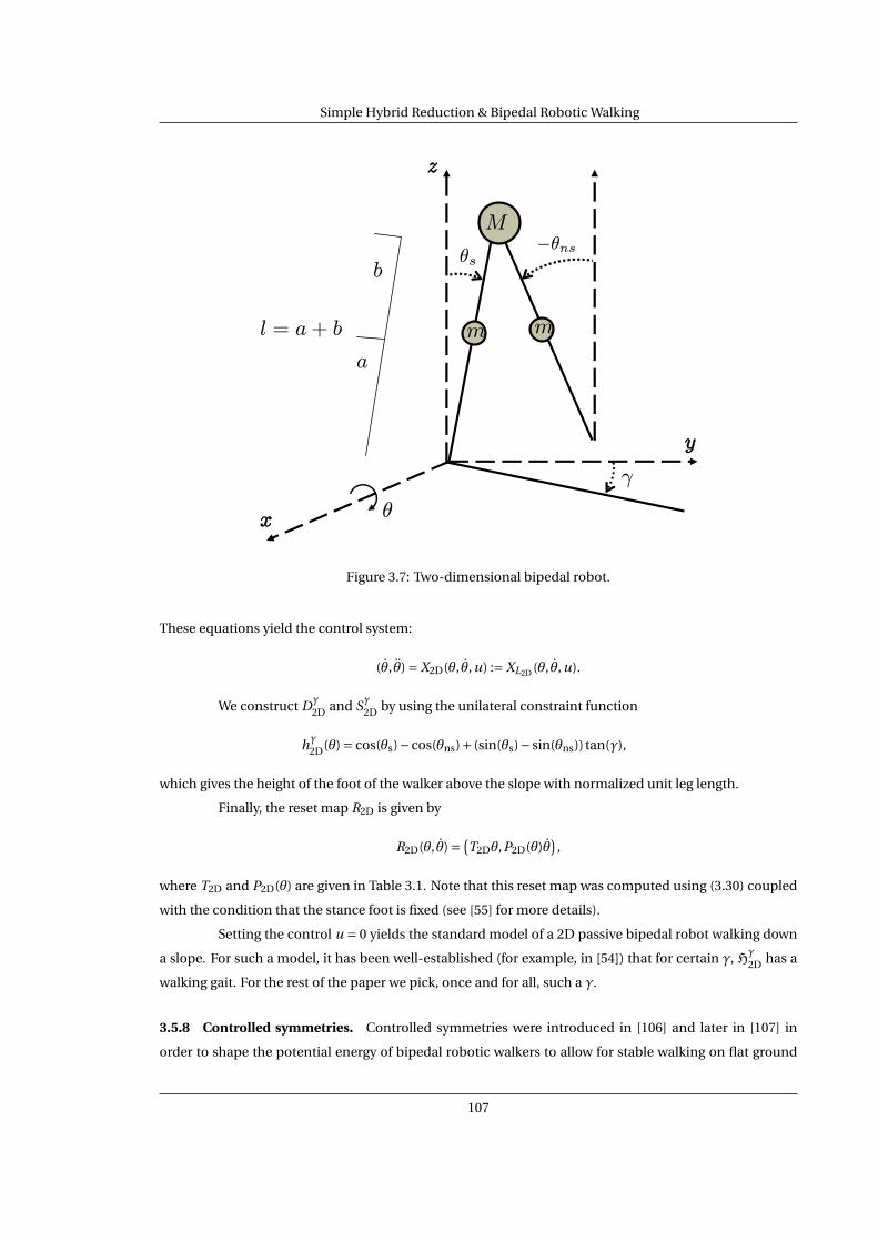
Simple Hybrid Reduction & Bipedal Robotic Walking
l = a+ b
b
a
M
m m
y
z
x
θs−θns
θ
γ
Figure 3.7: Two-dimensional bipedal robot.
These equations yield the control system:
(θ, θ) = X2D(θ, θ, u) := XL2D (θ, θ, u).
We construct Dγ
2D and Sγ2D by using the unilateral constraint function
hγ
2D(θ) = cos(θs)−cos(θns)+ (sin(θs)− sin(θns)) tan(γ),
which gives the height of the foot of the walker above the slope with normalized unit leg length.
Finally, the reset map R2D is given by
R2D(θ, θ) = (T2Dθ,P2D(θ)θ
),
where T2D and P2D(θ) are given in Table 3.1. Note that this reset map was computed using (3.30) coupled
with the condition that the stance foot is fixed (see [55] for more details).
Setting the control u = 0 yields the standard model of a 2D passive bipedal robot walking down
a slope. For such a model, it has been well-established (for example, in [54]) that for certain γ, Hγ
2D has a
walking gait. For the rest of the paper we pick, once and for all, such a γ.
3.5.8 Controlled symmetries. Controlled symmetries were introduced in [106] and later in [107] in
order to shape the potential energy of bipedal robotic walkers to allow for stable walking on flat ground
107

Simple Hybrid Reduction & Bipedal Robotic Walking
Additional equations for H2D:
M2D(θ) = l2m
4 − l2m cos(θs−θns)2
− l2m cos(θs−θns)2
l2m4 + l2(m +M)
V2D(θ) = 1
2g l((3m +2M)cos(θs)−m cos(θns))
B2D = −1 0
1 1
T2D = 0 1
1 0
P2D(θ) = 1
−3m −4M +2m cos(2(θs −θns)) 2m cos(θns −θs) m −4(m +M)cos(2(θns −θs))
m −2(m +2M)cos(θns −θs)
Additional equations for H3D:
m3D(θ) = 1
8(l2(6m +4M)+ l2(m cos(2θns)
−8m cos(θns)cos(θs)+ (5m +4M)cos(2θs))
V3D(θ,ϕ) = V2D(θ)cos(ϕ)
p3D(θ) = −m cos(2θns)+8(m +M)cos(θns)cos(θs)−m(2+cos(2θs))
6m +4M + (5m +4M)cos(2θns)−8m cos(θns)cos(θs)+m cos(2θs)
Table 3.1: Additional equations for H2D and H3D.
based on stable walking down a slope. We will briefly apply the results of this work to derive a feedback
control law that yields a hybrid system, Hs2D, with stable walking gaits on flat ground.
The main idea of [107] is that inherent symmetries in Hγ
2D can be used to “rotate the world” (via
a group action) to allow for walking on flat ground. Specifically, we have a group action Φ :S1×Q2D →Q2D
denoted by:
Φ(γ,θ) := θns −γ
θs −γ
,
for γ ∈S1. Using this, define the following feedback control law:
u = Kγ
2D(θ) = B−12D
∂
∂θ
(V2D(θ)−V2D(Φ(γ,θ))
).
108

Simple Hybrid Reduction & Bipedal Robotic Walking
Applying this control law to the control system (q, q) = X2D(θ, θ, u) yields the dynamical system:
(θ, θ) = Xγ
2D(θ, θ) := X2D(θ, θ,Kγ
2D(θ))
which is just the vector field associated to the Lagrangian
Lγ2D(θ, θ) = 1
2θT M2D(θ)θ−V γ
2D(θ),
where V γ
2D(θ) := V2D(Φ(γ,θ)). That is, Xγ
2D = XLγ
2D.
Now define, for some γ that results in stable passive walking for Hγ
2D,
Hs2D := (D0
2D,S02D,R2D,Xγ
2D),
which is a Lagrangian hybrid system. In particular, it is related to Hγ
2D via the main result of [107] as
follows:
Theorem 3.8. Let
εHγ
2D = (Λ, I , (θi , θi )i∈Λ)
be a hybrid flow of Hγ
2D (with u = 0), then
εHs2D = (Λ, I , (Φ(γ,θi ), θi )i∈Λ)
is a hybrid flow of Hs2D.
Theorem 3.8 implies that if Hγ
2D walks (stably) on a slope, then Hs2D walks (stably) on flat ground.
3.5.d Functional Routhian Reduction Applied to 3D Bipedal Walkers
In this section we construct a control law that results in stable walking for a simple model of
a three-dimensional bipedal robotic walker. In order to achieve this goal, we shape the potential energy
of this model via feedback control so that when hybrid functional Routhian reduction is carried out, the
result is the stable 2D walker introduced in the previous section. We utilize Theorem 3.7 to demonstrate
that this implies that the 3D walker has a walking gait on flat ground (in three dimensions).
3.5.9 3D biped model. We now introduce the model describing a controlled bipedal robot walking in
three-dimensions on flat ground, i.e., we will explicitly construct the controlled hybrid system describing
this system:
H3D = (D3D,S3D,R3D,X3D).
The configuration space for the 3D biped is Q3D = T2 ×S and the Lagrangian describing this
system is given by:
L3D(θ, θ,ϕ,ϕ) = 1
2
θ
ϕ
T M2D(θ) 0
0 m3D(θ)
θ
ϕ
−V3D(θ,ϕ), (3.40)
109

Simple Hybrid Reduction & Bipedal Robotic Walking
l = a+ b
b
a
M
m m
y
z
x
−θnsθs
θ
x0
z0
−ϕ
ϕ
Figure 3.8: Three-dimensional bipedal robot.
where m3D(θ) and V3D(θ,ϕ) are given in the Table 3.1. Note that, referring to the notation introduced in
(3.31), Mθ(θ) = M2D(θ) and Mϕ(θ) = m3D(θ). Also note that L3D is nearly cyclic; it is only the potential
energy that prevents its cyclicity. This will motivate the use of a control law that shapes this potential
energy.
Using the controlled Euler-Lagrange equations, the dynamics for the walker are given by
M3D(q)q +C3D(q, q)q +N3D(q) = B3Du
with q = (θ,ϕ) and
B3D = B2D 0
0 1
.
These equations yield the control system:
(q, q) = X3D(q, q, u) := XL3D (q, q, u).
We construct D3D and S3D by utilizing the unilateral constraint function
h3D(θ,ϕ) = h02D(θ) = cos(θs)−cos(θns).
This function gives the normalized height of the foot of the walker above the ground with the implicit
assumption that ϕ ∈ (−π/2,π/2) (which allows us to disregard the scaling factor cos(ϕ) that would have
been present). The result is that h3D is cyclic.
110

Simple Hybrid Reduction & Bipedal Robotic Walking
Finally, the reset map R3D is given by
R3D(θ, θ,ϕ,ϕ) = (T2Dθ,P2D(θ)θ,ϕ, p3D(θ)ϕ
)where p3D(θ) is given in Table 3.1. Note that this map was again computed using (3.30) coupled with the
condition that the stance foot is fixed.
3.5.10 Control law construction. We now proceed to construct a feedback control law for H3D that
makes this hybrid system an almost-cyclic Lagrangian hybrid system, Hα3D. We will then demonstrate,
using Theorem 3.7, that Hα3D has a walking gait by relating it to Hs
2D.
Define the feedback control law parameterized by α ∈R:
u = Kα3D(q) = B−1
3D∂
∂q
(V3D(q)−V γ
2D(θ)+ 1
2
α2ϕ2
m3D(θ)
).
Applying this control law to the control system (q, q) = X3D(q, q, u) yields the dynamical system:
(q, q) = Xα3D(q, q) := X3D(q, q,Kα
3D(q)),
which is just the vector field associated to the almost-cyclic Lagrangian
Lα3D(θ, θ,ϕ,ϕ) = 1
2
θ
ϕ
T M2D(θ) 0
0 m3D(θ)
θ
ϕ
−Vα3D(θ,ϕ), (3.41)
where
Vα3D(θ,ϕ) = V γ
2D(θ)− 1
2
α2ϕ2
m3D(θ).
That is, Xα3D = XLα3D
.
We now define
Hα3D := (D3D,S3D,R3D,Xα
3D),
which is a Lagrangian hybrid system.
3.5.11 Applying hybrid functional Routhian reduction. Using the methods outlined in Subsection
3.5.b, there is a momentum map J3D : TQ3D →R given by
J3D(θ, θ,ϕ,ϕ) = m3D(θ)ϕ,
and so setting J3D(θ, θ,ϕ,ϕ) =λ(ϕ) =−αϕ implies that
ϕ=− αϕ
m3D(θ).
The importance of Hα3D is illustrated by the following theorem.
111

Simple Hybrid Reduction & Bipedal Robotic Walking
Theorem 3.9. Hα3D is an almost-cyclic Lagrangian hybrid system. Moreover, the following diagram com-
mutes:
Rk
S3DR3D -
J3D|S3D
-
D3D
J3D|D3D
S2D
π
? R2D - D2D
π
?
Therefore, Hs2D is the functional Routhian hybrid system associated with Hα
3D.
Proof. By the construction of Hα3D, one need only show that:
m3D(θ) = m3D(T2Dθ)p3D(θ),
which follows by direct calculation.
This result allows us to prove—using Theorem 3.7—that the control law used to construct Hα3D
in fact results in walking in three-dimensions when α> 0.
Theorem 3.10.
εHα3D = (Λ, I , (θi , θi ,ϕi ,ϕi )i∈Λ)
is a hybrid flow of Hα3D with
ϕ0(τ0) =− αϕ0(τ0)
m3D(θ0(τ0)), (3.42)
if and only if
εHs2D = (Λ, I , θi , θi i∈Λ)
is a hybrid flow of Hs2D and (ϕi ,ϕi )i∈Λ satisfies:
ϕi (t ) =− αϕi (t )
m3D(θi (t )), ϕi+1(τi+1) =ϕi (τi+1). (3.43)
Proof. Follows from Theorem 3.7 and Theorem 3.9.
3.5.12 Simulation results. We conclude this Chapter by discussing the implications of Theorem 3.10.
Moreover, we demonstrate the usefulness of this result by showing through simulation that it does result
in walking the three-dimensions. To better visualize the following discussion, refer to Figure 3.11 for an
initial configuration of the robot and Figure 3.12 for a walking sequence of the robot.
Suppose that εHα3D = (Λ, I , (θi , θi ,ϕi ,ϕi )i∈Λ) is a hybrid flow of Hα
3D. If this hybrid flow has an
initial condition satisfying (3.42) with α> 0 and the corresponding hybrid flow, εHs2D = (Λ, I , θi , θi i∈Λ), of
Hs2D is a walking gait in 2D:
Λ=N, limi→∞
τi =∞, θi (τi ) = θi+1(τi+1),
112

Simple Hybrid Reduction & Bipedal Robotic Walking
Figure 3.9: θns, θs and ϕ over time for a stable walking gait and different initial values of ϕ.
then the result is walking in three-dimensions. This follows from the fact that θ and θ will have the same
behavior over time for the full-order system—the bipedal robot will walk. Moreover, since Theorem 3.10
implies that (3.43) holds, the walker stabilizes to the “upright” position. This follows from the fact that
the roll, ϕ, will tend to zero as time goes to infinity since (3.43) essentially defines a stable linear system
ϕ = −αϕ (because m3D(θi (t )) > 0 and α > 0), which controls the behavior of ϕ when (3.42) is satisfied.
This convergence can be seen in Figure 3.9.
Theorem 3.10 only implies that the 3D biped has walking gaits for hybrid flows with initial con-
ditions that satisfy (3.42); the set of all such initial conditions defines a region that is stable to the origin
(ϕ,ϕ) = (0,0), which corresponds to “upright” walking (see Figure 3.10). This illustrates that our control
law for the 3D biped is not a locally stabilizing controller (as would be the case if we were to linearize, see
[73]) but rather stabilizes a nonlinear subset of the initial conditions. It is possible to extend this region of
convergence by stabilizing to the manifold defined by
ϕ+ αϕ
m3D(θ)= 0.
This indicates that hybrid reduction can be used to stabilize a three-dimensional walker from a large set
of initial conditions.
113

Simple Hybrid Reduction & Bipedal Robotic Walking
Fig
ure
3.10
:Ph
ase
po
rtra
its
for
ast
able
wal
kin
gga
it.T
he
bla
ckre
gio
nsh
ows
the
init
ialc
on
dit
ion
so
fϕan
dϕ
that
con
verg
eto
the
ori
gin
.
114

Simple Hybrid Reduction & Bipedal Robotic Walking−
0.5
00.
5
0
1
2
3
4
0
0.2
0.4
0.6
0.81
xy
z
−0.
50
0.5
1
2
3
0
0.2
0.4
0.6
0.81
xy
z
1
Fig
ure
3.11
:Th
ein
itia
lco
nfi
gura
tio
no
fth
eb
iped
alro
bo
t.
115
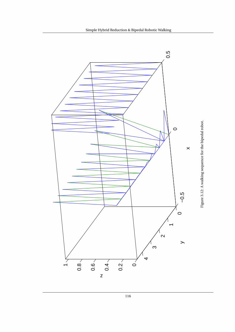
Simple Hybrid Reduction & Bipedal Robotic Walking
−0.
50
0.5
0
1
2
3
4
0
0.2
0.4
0.6
0.81
xy
z
−0.
50
0.5
1
2
3
0
0.2
0.4
0.6
0.81
xy
z
1
Fig
ure
3.12
:Aw
alki
ng
seq
uen
cefo
rth
eb
iped
alro
bo
t.
116

Chapter 4
Hybrid Geometric Mechanics
Mechanics, and the geometry thereof, plays a fundamental role in engineering. This chapter
gives a general outline on how to extend classical ideas from geometry and mechanics to a hybrid setting
through the use of hybrid objects.
The objects of study in geometry display the fundamental property of being categorical, i.e., they
reside in certain categories. Collections of geometric objects in a category relate to one another naturally,
i.e., morphisms between geometric objects in two diagrams extend naturally to morphisms between dia-
grams. The relationship between different classes of geometric objects is functorial, i.e. one can translate
from one class of geometric objects to another through the use of functors. Therefore, using the categori-
cal, natural and functorial nature of geometric objects, one can hybridize these objects. Specifically, given
a category C consisting of the geometric objects of interest, e.g., manifolds, Lie groups, Lie algebras, etc.,
one can form the “hybrid version” of these objects:
A : A →C,
with A either covariant or contravariant, i.e., (A ,A) is a hybrid or cohybrid object. We thus form the
category of hybrid or cohybrid objects, Hy(C) or CoHy(C), depending on the contravariance or covariance
of A. Using the functorial relationship between different categories of geometric objects, e.g., the functor
that associated to a Lie group its Lie algebra, we obtain functors between the categories of hybrid objects
of interest. Some of the hybrid objects, hybrid morphisms and functors between categories of hybrid
objects that will be introduced in this chapter can be seen in Table 4.1.
Recall from Chapter 3 that we were interested in answering the following question:
If it is possible to reduce the continuous components of a hybrid system, when is it possible toreduce the entire hybrid system?
In that chapter, we were only able to answer this question for simple hybrid systems. Using the framework
established by hybrid geometry, we will be able to answer this question for general hybrid systems. First,
we recall the classical reduction theorem.
117

Hybrid Geometric Mechanics
Important hybrid objects :
Hybrid vector space : V : V → VectR
Hybrid manifold : M : M → Man
Hybrid tanget bundle : T∗(M) : M → VectBundR
Hybrid differential k− forms : Ωk∗(M) : M → VectR
Hybrid de Rham cohomology : HndR∗(M) : M → VectR
Hybrid Lie group : G : G → LieGrp
Hybrid Lie algebra : g : G → LieAlg
Dual hybrid Lie algebra : g? : G → VectR
Hybrid isotropy group : G~µ : G → LieGrp
Hybrid orbit space : M///G : M → Top
Reduced hybrid phase space : M~µ : M → Man
Important hybrid morphisms :
Hybrid exterior derivative : ~d : Ωk∗(M)→ Ωk+1∗ (M)
Hybrid wedge product : − ~∧ − : Ωk∗(M)×Ωl∗(M)→ Ωk+l∗ (M)
Hybrid conjunction map : I~g : G→ G
Hybrid adjoint action : Ad~g : g→ g
Hybrid group action : ~Φ : G×M→ M
Hybrid infintesimal generator : ~ξM : M→ T∗(M)
Hybrid momentum map : ~J : M→ g?
Important functors :
Hybrid tangent bundle functor : Hy(T ) : Hy(Man) → Hy(VectBundR)
Hybrid k− form functor : Hy(Ωk ) : Hy(Man) → CoHy(VectR)
Hybrid Lie functor : Hy(Lie) : Hy(LieGrp) → Hy(LieAlg)
Dual vector space functor : Hy(( − )?) : Hy(VectR) → CoHy(VectR)
Table 4.1: Important hybrid objects, morphisms between hybrid objects and functors between categoriesof hybrid objects.
118

Hybrid Geometric Mechanics
Marsden mathematically describes, [86], the reduction theorem for classical mechanics as fol-
lows:
Given a symplectic manifold M (the phase space), there exists a symplectic manifold Mµ suchthat “Mµ inherits the symplectic structure from that of M, so it can be used as a new phase space.Also, dynamical trajectories of the Hamiltonian H on M determine corresponding trajectorieson the reduced space.”
Upon inspection, it is clear that a rather copious mathematical framework is needed to perform reduction:
there must be a Lie group G acting on the symplectic manifold M , and an Ad∗-equivariant momentum
map J : M → g∗, and the Hamiltonian H must be G-invariant.
Hybrid objects will allow us to generalize all of the ingredients necessary for reduction to a hy-
brid setting. The main result is the following hybrid reduction theorem:
Given a hybrid symplectic manifold M (the hybrid phase space), there exists a hybrid symplecticmanifold M~µ such that M~µ inherits the hybrid symplectic structure from that of M, so it can beused as a new hybrid phase space. Also, dynamical trajectories of the hybrid Hamiltonian H onM determine corresponding trajectories on the reduced hybrid space.
That is, if (M,~ω,H) is a hybrid Hamiltonian system (M is a hybrid manifold, ~ω is a hybrid symplectic form
on M and H is a hybrid Hamiltonian), then this theorem says that under certain conditions we can reduce
this hybrid Hamiltonian system to obtain a reduced hybrid Hamiltonian system (M~µ,~ω~µ,H~µ).
The hybrid reduction theorem can be used to explicitly reduce hybrid systems since we can
associate to a hybrid Hamiltonian system (Mııı ,~ω,H) a “classical” hybrid system H(Mııı ,~ω,H) (see Paragraph
2.1.2, Proposition 2.1 and Proposition 2.2). Therefore, the ability to reduce hybrid Hamiltonian systems
yields a method for reducing hybrid systems; graphically, the operation of “hybrid system reduction” is
defined by requiring the following diagram to commute:
(Mııı ,~ω,H)reduction- (Mııı
~µ,~ω~µ,H~µ)
H(Mııı ,~ω,H)
association? reduction- H(Mııı
~µ,~ω~µ,H~µ).
association?
Moreover, since this association is constructive in nature, the result is a concrete method for reducing
hybrid systems. Finally, the hybrid reduction theorem proven in this chapter can be used to show that
trajectories (or executions) of H(Mııı ,~ω,H) determine corresponding trajectories of H(Mııı~µ
,~ω~µ,H~µ).
The work on which this chapter builds is the same as that of Chapter 3; see the related work
paragraph in that chapter.
Examples will be sparse in this chapter as we believe that we have more than motivated the
importance of reduction in Chapter 3, especially given the application of reduction to bipedal walking.
We will utilize a simple example throughout the chapter in order to illustrate the concepts involved.
Running example. Throughout this chapter, we will consider a ball bouncing in two-dimensions; this
differs from the one-dimensional version introduced earlier as well as the three-dimensional version ball
119

Hybrid Geometric Mechanics
0.0
0.2
0.4
0.6
0.8
1.0
0 1 2 3 4 5 6 7 8 9 10
Position: x vs. y
Figure 4.1: A trajectory of the two-dimensional (completed) bouncing ball model.
bouncing on a sinusoidal surface. We will not use the standard model of this system (which has a single
domain) but rather the completed version of the system (obtained using the procedure outlined in Section
5.5 of Chapter 5) which allows the ball to “stop bouncing” after the Zeno point is reached; see Figure 4.1.
We introduce the model of this system directly as a categorical hybrid system rather than trans-
lating the definition from the standard definition as has been our custom. Since the goal is to define a
hybrid system, we first define its discrete structure.
Define M ball as the D-category given by the following diagram:
ab
M ball =
b
sab
?
tab
?
sas astas - s.
where “b” will correspond to the state where the ball is “bouncing” and “s” will correspond to the state
where the ball is “sliding.”
Define the hybrid manifold:
Mball : M ball →Man
by:
Mball(M ball
)=
Mballab
Mballb =R4
Mballsab
= ı?
∩
Mballtab
?
Mballsas
= ı⊃ Mball
as=R2
Mballtas
= id- Mball
s =R2
where here the coordinates onR4 are (x, y, px , py )T , the coordinates onR2 are (x, px )T , with Mballab
and Mballtab
120

Hybrid Geometric Mechanics
given by:
Mballab
=
x
y
px
py
∈R4 : y = 0 and py ≤ 0
,
Mballtab
(x,0, px , py ) =
x
0
px
−epy
,
with 0 ≤ e ≤ 1 the coefficient of restitution.
Finally, the hybrid system is given by (M ball,Mball,Xball) where
Xball = Xballb ,Xball
s ,
with:
Xballb (x, y, px , py ) = 1
m
px
py
0
−m2g
,
Xballs (x, px ) = 1
m
px
0
.
and m the mass of the ball.
4.1 Hybrid Differential Forms
In order to discuss the general geometric reduction of hybrid systems, we introduce hybrid dif-
ferential forms. The framework of hybrid objects makes this a relatively easy task, although it is nontrivial
as the constructions are not always the obvious ones. Note that we could first build up the general frame-
work of tensor bundles, etc., but since the construction is essentially the same, we proceed directly to the
notion of differential forms which is the main concept of interest.
Note that when dealing with hybrid differential forms, we are forced to deal with both covari-
ant and contravariant functors. To avoid confusion, we will explicitly state which type of functor we are
considering when necessary.
We refer the reader to [79] for any necessary background material.
4.1.1 Hybrid tangent bundles. We begin by discussing how one associates to a hybrid manifold its
hybrid tangent bundle. This will be useful for understanding later constructions.
121

Hybrid Geometric Mechanics
The process of associating a tangent bundle to a manifold defines a functor:
T : Man→VectBundR
where VectBundR is the category of (real) vector bundles. Specifically, we have T (M) = T M , where T M is
the tangent bundle of M ; implicit in this notation is the canonical projection π : T M → M that makes T M
into a vector bundle. In addition, for a morphism f of manifolds T f is the pushfoward of this function.
The functor T induces a functor:
Hy(T ) : Hy(Man) →Hy(VectBundR).
That is, for a hybrid manifold (M ,M), we can associate to this hybrid manifold its hybrid tangent bundle
(M ,T∗(M)) :=Hy(T )(M ,M),
where
T∗(M) : M →VectBundR
is given by, for every aα→ b in M ,
T∗(M)a := T MaT∗(M)α := T Mα- T∗(M)b := T Mb .
Here T Mα is the pushforward of Mα,
T Mα(p,X ) = (Mα(p),Tp Mα(X )),
for (p,X ) ∈ T Ma , i.e., for X ∈ Tp Ma and p ∈ Ma .
If (~F , ~f ) : (M ,M) → (N ,N) is a morphism of hybrid manifolds, then there is an induced mor-
phism:
Hy(T )(~F , ~f ) = (~F ,T∗(~f )) : Hy(T )(M ,M) = (M ,T∗(M)) → (N ,T∗(N))
between the hybrid tangent bundles of these hybrid manifolds as outlined in Paragraph 1.3.7.
4.1.2 Hybrid sections. Note that we have a natural transformation ~π : T∗(M)→ M, i.e., a hybrid mor-
phism:
(~IdM ,~π) : (M ,T∗(M)) → (M ,M),
called the canonical hybrid projection map, and given objectwise by the natural projection, i.e., ~πa :
T∗(M)a = T Ma → Ma .
We can consider sections of the hybrid tangent bundle of a hybrid manifold:
Γ(M) := ~X : M→ T∗(M) : ~π• ~X = ~idM,
which in fact defines a collection of vector fields (of a very special form) on the hybrid manifold (M ,M),
i.e., associated to the hybrid section, ~X , we have the collection of vector fields X := ~Xbb∈V(M ). That being
said, hybrid sections are typically not of interest as they are too restrictive.
122

Hybrid Geometric Mechanics
4.1.3 Differential forms. Let M be a manifold and let Λk (M) be the vector bundle consisting of all
alternating tensors, i.e., we have a canonical projection map π : Λk (M) → M . A section of this vector
bundle
ω : M →Λk (M) s.t. πω= idM
is a differential k-form or just a k-form. The set of all differential k-forms is denoted by:
Ωk (M) = ω : M →Λk (M) :πω= idM .
The process of associating to a manifold its differential k-forms induces a contravariant functor:
Ωk : Man→VectR,
where for f : M → N ,
Ωk ( f ) : Ωk (N) →Ωk (M)
is the pullback of f given by, for ω ∈Ωk (N), p ∈ M and X1, . . .Xk ∈ TpM ,
Ωk ( f )(ω)p(X1, . . . ,Xk ) :=ω f (p)(Tp f (X1), . . . ,Tp f (Xk )),
where Tp f (X1), . . . ,Tp f (Xk ) ∈ T f (p)N .
Remark 4.1. Note that Ωk ( f ), termed the pullback of the function f , is typically denoted by f ∗. We opt for
the non-standard notation because it demonstrates that the pullback of a function is functorally obtained
from the original function. In addition, it avoids the proliferation of ∗’s that would be inevitable due to
the notation utilized to denote the pushforward of a functor.
4.1.4 Hybrid differential forms. The contravariant functor Ωk induces a contravariant functor:
Hy(Ωk ) : Hy(Man) →CoHy(VectR).
For a hybrid manifold (M ,M),
Hy(Ωk )(M ,M) := (M ,Ωk∗(M)),
withΩk∗(M) : M →VectR a contravariant functor given on objects byΩk∗(M)a =Ωk (Ma) and on morphisms
α : a → b in M by
Ωk∗(M)α =Ωk (Mα) : Ωk
∗(M)b →Ωk∗(M)a .
For a morphism (~F , ~f ) : (M ,M) → (N ,N) in Hy(Man), we have the corresponding morphism in CoHy(VectR):
Hy(Ωk )(~F , ~f ) := (~Fop,Ωk∗(~f )) : (N ,Ωk
∗(N)) → (M ,Ωk∗(M)),
where ~Fop : N → M is the morphism in Dcatop corresponding to ~F and Ωk∗(~f ) : ~F∗(Ωk∗(N))→Ωk∗(M) in
M VectR. In particular, there is the following relationship
Ma
~fa- N~F (a)
Mb
Mα
? ~fb- N~F (b)
N~F (α)
?
7→
Ωk (Ma) Ωk (~fa)
Ωk (N~F (a))
Ωk (Mb)
Ωk (Mα)6
Ωk (~fb)
Ωk (N~F (b))
Ωk (N~F (α))6
123

Hybrid Geometric Mechanics
in Man and VectR, respectively, for every α : a → b in M .
We are especially interested in elements of the cohybrid object (M ,Ωk∗(M)).
Definition 4.1. Let (M ,M) be a hybrid manifold. A hybrid differential k-form is an element of the cohy-
brid object (M ,Ωk∗(M)), i.e.,
~ω ∈ (M ,Ωk∗(M)).
Therefore, a hybrid differential k-form must satisfy:
¦ ~ωa ∈Ωk (Ma), i.e, ~ωa is a differential k-form,
¦ Ωk (Mα)(~ωb) = ~ωa for all α : a → b in M .
Notation 4.1. To simplify notation, when referring to elements of (M ,Ωk∗(M)) we will often write ~ω ∈Ωk∗(M) since we will always be considering the same D-category M .
4.1.5 Hybrid symplectic manifolds. The formulation of hybrid differential forms allows us to define
hybrid symplectic manifolds. Note that the definition of a hybrid symplectic manifold is not the most
obvious one—we do not require a hybrid differential 2-form to be objectwise a symplectic form.
Definition 4.2. A hybrid symplectic manifold is a hybrid manifold (M ,M) together with a hybrid 2-form
~ω ∈Ω2(M) such that ~ωb is smooth, closed and nondegenerate, i.e., a symplectic form, for all b ∈V(M ).
Example 4.1. On the hybrid manifold (M ball,Mball), we will consider the canonical hybrid symplectic
form, i.e., ~ωball is specified by ~ωballb and ~ωball
s , which are the standard symplectic forms on R4 and R2,
respectively, with
~ωballas
:= ~ωballs , ~ωball
ab:=Ω2(ı)(~ωball
b ).
A simple calculation verifies that:
Ω2(ı)(~ωballb ) = ~ωball
as, ~ωball
ab=Ω2(Mball
tab)(~ωball
b ),
so Definition 4.2 is satisfied and (M ball,Mball,~ωball) is a hybrid symplectic manifold.
We are now interested in defining some elementary operations on Ωk∗(M).
4.1.6 Hybrid exterior derivatives. For a hybrid manifold (M ,M), the hybrid exterior derivative is a nat-
ural transformation:
~d : Ωk∗(M)
→Ωk+1∗ (M)
defined for all k ∈N. It is given on objects a of D by:
~da : Ωk (Ma)→Ωk+1(Ma),
where ~da is the exterior derivative on Ma . It follows that the hybrid exterior derivative is a hybrid linear
map, i.e., that it is objectwise linear. Moreover, if ~ω ∈Ωk∗(M), then ~d(~ω) ∈Ωk+1∗ (M) where ~d(~ω)a = ~da(~ωa).
The hybrid exterior derivative displays the following obvious and yet important property:
124

Hybrid Geometric Mechanics
Lemma 4.1. ~d • ~d =~0.
In the preceding lemma,~0 is a natural transformation that is objectwise zero.
4.1.7 Hybrid wedge product. For a hybrid manifold (M ,M), the hybrid wedge product or hybrid inte-
rior product is a natural transformation:
− ~∧ − : Ωk∗(M)×Ωl
∗(M)→Ωk+l
∗ (M)
such that for all a ∈Ob(M ), the following map:
− ~∧a − : Ωk (Ma)×Ωl (Ma)→Ωk+l (Ma)
is the wedge product. It follows that if ~ω ∈ Ωk∗(M) and ~η ∈ Ωk∗(M) then ~ω~∧~η ∈ Ωk+l∗ (M) where (~ω~∧~η)a :=~ωa~∧a~ηa .
Hybrid wedge products and hybrid exterior derivatives are related through the following lemma.
Lemma 4.2. For ~ω ∈Ωk∗(M) and ~η ∈Ωl∗(M),
~d(~ω~∧~η) = ~d(~ω)~∧~η+ (−1)k~ω~∧ ~d(~η),
where the addition in this expression is preformed objectwise.
To provide an example of some of the other constructions that can be carried out using cate-
gories of hybrid objects and categories of cohybrid objects, we briefly discuss de Rham cohomology.
4.1.8 Hybrid de Rham cohomology. For a smooth manifold M , the exterior derivative yields a cochain
complex in the category of vector spaces:
00- Ω0(M)
d - · · · d- Ωn−1(M)d- Ωn(M)
d- Ωn+1(M)d - · · ·
denoted by (Ω•(M), d). Consider the linear subspaces:
Z n(M) := Ker(d : Ωn(M) →Ωn+1(M))
= ω ∈Ωn(M) : d(ω) = 0,
Bn(M) := Im(d : Ωn−1(M) →Ωn(M)))
= ω ∈Ωn(M) : ∃ η ∈Ωn−1(M) s.t. d(η) =ω.
The nth de Rham cohomology group of M is defined to be the cohomology of the cohain complex (Ω•(M), d):
HndR(M) = Hn(Ω•(M)) = Z n(M)
Bn(M).
Note that taking the de Rham cohomology of a manifold results in a contravariant functor:
HndR : Man→VectR
125

Hybrid Geometric Mechanics
defined for each n ∈N.
For a hybrid manifold (M ,M), the de Rham cohomology functor induces a contravariant func-
tor:
Hy(HndR) : Hy(Man) →CoHy(VectR).
That is, for a hybrid manifold (M ,M),
Hy(HndR)(M ,M) := (M ,Hn
dR∗(M)),
is called the nth hybrid de Rham cohomology group of (M ,M).
Therefore, we are able to do “hybrid de Rham cohomology.” More on the homology of hybrid
systems can be found in [14].
4.2 Hybrid Lie Groups and Algebras
We are interested in studying the relationship between hybrid Lie groups and hybrid Lie algebras
via the relationship between Lie groups and Lie algebras.
4.2.1 Hybrid Lie groups. The category of Lie groups, LieGrp, has as
Objects: Lie groups, i.e., groups that are also (smooth) manifolds such that multiplicationand inversion define smooth maps,
Morphisms: Smooth maps that are also group homomorphisms.
A hybrid Lie group is a hybrid object over the category of Lie groups, LieGrp, i.e., a pair (G ,G) where
G : G → LieGrp .
An element of a hybrid Lie group, ~g ∈ (G ,G), must satisfy the following properties:
¦ ~ga ∈ Ga for all objects a of G ,
¦ ~gb = Gα(~ga) for all α : a → b in G .
In particular, every element of (G ,G) has an inverse, ~g−1, defined objectwise to be the inverse of ~ga , i.e.,
~g−1a · ~ga = eGa = ~ga · ~g−1
a
where eGa is the identity element of Ga .
4.2.2 Lie algebras. Recall that a Lie algebra g is a vector space together with a binary operation:
[ − , − ] : g×g → g
(X ,Y ) 7→ [X ,Y ],
126

Hybrid Geometric Mechanics
called the Lie bracket. This bracket must satisfy, for all X ,Y ,Z ∈ g:
Bilinearity. For all r, w ∈R,
[rX +wY ,Z ] = r [X ,Z ]+w[Y ,Z ]
[Z , rX +wY ] = r [Z ,X ]+w[Z ,Y ]
Antisymmetry.
[X ,Y ] =−[Y ,X ]
Jacobi Identity.
[X , [Y ,Z ]]+ [Y , [Z ,X ]]+ [Z , [X ,Y ]] = 0.
A morphism of Lie algebras is a linear map A : g→ h such that:
A([X ,Y ]) = [A(X ), A(Y )].
We have thus defined the category of Lie algebras, LieAlg.
4.2.3 Hybrid Lie algebras. We could directly define a hybrid Lie algebra as a hybrid object over the
category of Lie algebras. We opt for a more circuitous route in order to demonstrate that hybrid objects
can often be defined using more “fundamental” information and that, in fact, the end result is the same.
A hybrid Lie algebra is a hybrid vector space (G ,g),
g : G →VectR
together with a natural transformation:
−−−−−−→[ − , − ] : g×g
→g
where the product is the product of functors given on objects and morphisms by (g×g)a = ga ×ga and
(g×g)α =gα×gα. That is, it is the product in VectGR which we know exists by Proposition A.4. In addition,
we require that for every object a of G , the corresponding binary operation:
−−−−−−→[ − , − ]a : ga ×ga →ga
satisfies the bilinearity, antisymmetry and Jacobi identities, i.e., it is a Lie bracket.
The following results say that this is in fact the “correct” definition of a hybrid Lie algebra:
Proposition 4.1. A hybrid object (G ,g) over VectR is a hybrid Lie algebra iff it is a hybrid object over LieAlg,
g : G → LieAlg .
127

Hybrid Geometric Mechanics
Proof. Beginning with a hybrid Lie algebra (G ,g), it is clear that ga is a Lie algebra. Therefore, we must
only verify that gα is a Lie algebra homomorphism. This follows from the commutativity of the diagram:
ga ×ga
−−−−−−→[ − , − ]a- ga
gb ×gb
gα×gα
? −−−−−−→[ − , − ]b- gb
gα
?
The converse direction is equally straightforward.
4.2.4 The Lie functor. The Lie functor is the functor:
Lie : LieGrp→ LieAlg,
given on objects by associating to a Lie group G its Lie algebra:
Lie(G) = TeG G ,
where TeG G is the tangent space at the identity element of G . Note that Lie(G) is isomorphic to (and could
be defined as) the set of all left-invariant vector fields on G . For a morphism f : G → H ,
Lie( f ) := TeG f : Lie(G) → Lie(H).
Note that Lie(G) is often denoted by g.
The Lie functor yields a functor between categories of hybrid objects:
Hy(Lie) : Hy(LieGrp) →Hy(LieAlg).
For a hybrid Lie group (G ,G), we will denote its corresponding hybrid Lie algebra by
Hy(Lie)(G ,G) := (G ,g),
and for a morphism of hybrid Lie groups (~F , ~f ) : (G ,G) → (H ,H) we obtain a morphism of hybrid Lie
algebras:
Hy(Lie)(~F , ~f ) := (~F ,Lie∗(~f )) : (G ,g) → (H ,h).
We know that this is a hybrid vector space, g : G → VectR, and so an element of (G ,g), which we denote
by ~ξ ∈ (G ,g) or just ~ξ ∈ g when the underlying D-category is clear from context, is a hybrid vector (as
introduced in Example 1.21) and so must satisfy:
¦ ~ξa ∈ga for all objects a of G , i.e., ~ξa is a vector,
¦ ~ξb =gα(~ξa) for all α : a → b in G .
In addition, we know from Example 1.21 that the set of elements of (G ,g),
ElemHy(LieAlg)(G ,g)
form a vector space. In fact, it is clear from Proposition 4.1 that the elements of (G ,g) form a Lie algebra.
128

Hybrid Geometric Mechanics
4.2.5 The dual to a hybrid Lie algebra. As discussed in Example 1.22, the functor that associates to a
vector space its dual induces a functor between categories of hybrid and cohybrid objects:
Hy(( − )?) : Hy(VectR) →CoHy(VectR).
Through this functor we obtain the dual to a hybrid Lie algebra (G ,g), which is the cohybrid object:
(G ,g?) :=Hy(( − )?)(G ,g).
It follows from Example 1.23 that an element of the cohybrid object (G ,g?), ~µ ∈ (G ,g?) or just ~µ ∈g?, is a
hybrid covector and thus must satisfy:
¦ ~µa ∈g?a for all objects a of G , i.e., ~µa : ga →R is a covector,
¦ g?α(~µb) = ~µa , i.e., ~µb gα = ~µa , for all α : a → b in G .
This implies that ~µ corresponds to a natural transformation ~µ : G→∆G (R).
Example 4.2. Returning to the bouncing ball, define a hybrid Lie group
Gball : M ball → LieGrp
by
Gballab
=RGball(M ball) =
Gballb =R
Gballsab
= id?
Gballtab
= id?
Gball
sas= id
Gballas
=RGball
tas= id
- Gballs =R.
That is, Gball =∆M ball (R). Note that in this case gball = Gball and (gball)? =∆opM ball (R).
4.2.6 The hybrid adjoint action. Let G be a Lie group and g ∈ G . The conjunction map is defined to
be a map Ig : G → G with Ig (h) = g hg−1 for h ∈ G . Utilizing the Lie functor, we obtain a Lie algebra
homomorphism:
Adg := Lie(Ig ) : g→ g,
which is termed the adjoint action. The functor that associates to a vector space its dual, ( − )?, yields a
morphism of vector spaces:
Ad?g : g? → g?
termed the coadjoint action.
The framework of hybrid objects allows adjoint and coadjoint actions to be easily generalized to
a hybrid setting. Given an element ~g ∈ (G ,G), we obtain a natural transformation:
I~g : G→ G
129

Hybrid Geometric Mechanics
defined objectwise by (I~g )a = I~ga . It is easy to verify that this in fact defines a natural transformation.
Utilizing the functor Hy(Lie) we obtain the hybrid adjoint action, i.e., a natural transformation:
Ad~g := Lie∗(I~g ) : g→g,
wherein it follows that (Ad~g )a = Ad~ga . Finally, utilizing the functor that associates to a hybrid vector space
its dual, Hy(( − )?), we obtain the hybrid coadjoint action, i.e., a natural transformation:
Ad?~g : g? →g?,
It follows that (Ad?~g )a = Ad?
~ga.
4.2.7 The hybrid isotropy subgroups. For a Lie group G , the isotropy subgroup under the coadjoint
action is given by, for µ ∈ g?,
Gµ = g ∈G : Ad?g−1 (µ) =µ.
For ~µ ∈ (G ,g?), define the hybrid isotropy group as the hybrid Lie group
G~µ : G → LieGrp
defined on objects and morphisms of G by:
(G~µ)a = (Ga)~µa , (G~µ)α = (Gα)|(G~µ)a .
We must verify that:
Proposition 4.2. (G ,G~µ) is a hybrid Lie group.
Proof. We need to show that
Ad?g−1 (~µa) = ~µa ⇒ Ad?
Gα(g−1)(~µb) = ~µb .
Since ~µ ∈ (G ,g?), i.e., g?α(~µb) = ~µa , this is equivalent to showing that:
g?α(Ad?
Gα(g−1)(~µb)) = ~µa .
First note that
AdGα(g−1) gα = TeGb(IGα(g−1))TeGa
(Gα)
= TeGa(IGα(g−1) Gα)
= TeGa(Gα Ig−1 )
= TeGa(Gα)TeGa
(Ig−1 )
= gα Adg−1 .
130

Hybrid Geometric Mechanics
This implies that
g?α(Ad?
Gα(g−1)(~µb)) = ~µb AdGα(g−1) gα
= ~µb gα Adg−1
= g?α(~µb)Adg−1
= Ad?g−1 (g?
α(~µb))
= Ad?g−1 (~µa)
yielding the desired result.
4.3 Hybrid Momentum Maps
We now switch our focus to hybrid reduction. Utilizing the constructions of the previous section,
we generalize reduction to a hybrid setting. In order to achieve this goal, we begin by introducing hybrid
momentum maps.
Momentum maps make explicit the conserved quantities of a Hamiltonian system. Hybrid mo-
mentum maps serve the same function, except that they define a set of conserved quantities. In order to
introduce hybrid momentum maps, it is first necessary to introduce the notion of hybrid symmetries, i.e.,
a hybrid action of a hybrid Lie group on a hybrid manifold. When such hybrid symmetries exist, along
with a momentum map, we are able to “divide” out by these symmetries to obtain the reduced hybrid
phase space.
We assume a basic knowledge of classical reduction throughout the rest of this chapter. We refer
the reader to the excellent reference [4] for any missing details.
Notation 4.2. We now fix a D-category D. We will assume that all hybrid objects have D as their underlying
discrete component except when discussing trajectories.
4.3.1 Hybrid group actions. For G : D → LieGrp and M : D →Man, define the hybrid manifold G×M :
D →Man as the product of G and M in ManD , i.e., on objects and morphisms:
(G×M)a := Ga ×Ma , (G×M)α := (Gα,Mα).
A hybrid group action or hybrid action is a natural transformation
~Φ : G×M→ M, (4.1)
that is objectwise a group action:
¦ For all p ∈ Ma , ~Φa(eGa , p) = p,
¦ For every g , h ∈ Ga , ~Φa(g ,~Φa(h, p)) = ~Φa(g h, p).
131

Hybrid Geometric Mechanics
We say that a hybrid group action is free if ~Φ is objectwise free and proper if it is objectwise proper.
For ~g ∈ G, we can associate to this action a hybrid diffeomorphism (a natural isomorphism)
~Φ~g : M→ M (4.2)
defined objectwise, for p ∈ Ma , by (~Φ~g )a(p) := ~Φa(~ga , p). Since ~Φ~g is a natural transformation, we have
Mα ~Φa(~ga , p) = ~Φb(Gα(~ga),Mα(p)), (4.3)
which is a form of equivariance; in the case when Ga = Gb and Gα = id, this condition says that Mα is
equivariant with respect to these actions.
Recall that in Definition 4.2 we introduced the definition of a hybrid symplectic manifold (M,~ω).
Definition 4.3. Let (M,~ω) be a hybrid symplectic manifold. A hybrid action ~Φ : G×M→ M is a symplectic
hybrid action if for the hybrid diffeomorphism ~Φ~g : M→ M,
Ω2∗(~Φ~g )(~ω) = ~ω
for each ~g ∈ G.
4.3.2 Hybrid orbit spaces. For a hybrid manifold M with a hybrid group G acting on it, let Ma/Ga be
the orbit space of the action ~Φa of Ga on Ma ; if p ∈ Ma , we denote the elements of this space by [p]. Define
the hybrid topological space
M///G : D →Top, (4.4)
defined on objects and morphisms of D by M///Ga := Ma/Ga and M///Gα([p]) := [Mα(p)], which is well-
defined by (4.3).
Proposition 4.3. If ~Φ : G×M→ M is a free and proper hybrid action, then M///G is a hybrid manifold, i.e.,
M///G : D →Man. Moreover, there is a hybrid submersion:
~π : M→ M///G.
That is, ~π is a natural transformation that is objectwise a submersion.
Proof. Define a natural transformation ~π : M → M///G by setting ~πa(p) := [p]; this is a natural transforma-
tion since
M///Gα ~πa(p) = M///Gα([p]) = [Mα(p)] = ~πb Mα(p).
By the definition of free and proper hybrid actions—they are objectwise free and proper—it follows that
Ma/Ga is a smooth manifold for every object a of D, and ~π is objectwise a submersion.
132

Hybrid Geometric Mechanics
Therefore, we need only verify that M///Gα is smooth for all morphisms α of D. This follows,
however, from the naturality of ~π, i.e., we have the following commuting diagram
MaMα - Mb
M///Ga
~πa
? M///Gα- M///Gb
~πb
?
and ~πb Mα is smooth so M///Gα ~πa must be smooth, or M///Gα must be smooth.
4.3.3 Hybrid infinitesimal generators of hybrid actions. Suppose there is a hybrid action ~Φ : G×M→
M. Then we can use this hybrid action to define a hybrid section of the hybrid tangent bundle of M for
every element ~ξ ∈g.
Define the infinitesimal generator of the hybrid action ~Φ corresponding to ~ξ ∈g by
~ξM : M→ T∗(M) (4.5)
which is given objectwise by
(~ξM)a(p) := d
dt~Φa(exp(t~ξa), p)
∣∣∣∣t=0
for p ∈ Ma .
Lemma 4.3. ~ξM is a hybrid section of the hybrid tangent bundle of M.
Proof. We need to show that for every diagram α : a → b in D
T∗(M)α (~ξM)a = (~ξM)b Mα.
First note that since ~ξ ∈g, i.e., gα(~ξa) = ~ξb , we have (by the properties of the exponential map, cf. [79]),
Gα(exp(t~ξa)) = exp(t TeGaGα(~ξa))
= exp(tgα(~ξa))
= exp(t~ξb).
Moreover, by (4.3),
Mα ~Φa(exp(t~ξa), p) = ~Φb(Gα(exp(t~ξa)),Mα(p))
= ~Φb(exp(t~ξb),Mα(p)).
Finally, for every p ∈ Ma , we have
Tp Mα (~ξM)a(p) = Tp Mα d
dt~Φa(exp(t~ξa), p)
∣∣∣∣t=0
= d
dt
(Mα ~Φa(exp(t~ξa), p)
)∣∣∣∣t=0
= d
dt~Φb(exp(t~ξb),Mα(p))
∣∣∣∣t=0
= (~ξM)b(Mα(p)).
133

Hybrid Geometric Mechanics
4.3.4 Hybrid regular values. Consider a natural transformation ~J : M→ g?; since M is covariant and
g? is contravariant, this implies (see Table 1.2) that the following diagram
Ma~Ja - g?
a
Mb
Mα
? ~Jb - g?b
g?α
6(4.6)
must commute for all α : a → b in D.
Definition 4.4. We say that ~µ ∈g? is a hybrid regular value of ~J if
1. ~µa ∈g?a is a regular value of ~Ja : Ma →g?
a for all objects a of D,
2. ~µb = ~Jb Mα(p) for all α : a → b in D and p ∈ Ma such that ~Ja(p) = ~µa .
4.3.5 The hybrid manifold J−−−111(((~µµµ))). Given a hybrid regular value ~µ ∈g?, define a hybrid manifold
J−−−111(((~µµµ))) : D →Man (4.7)
given on objects and morphisms of D by
J−−−111(((~µµµ)))a := ~J−1a (~µa), J−−−111(((~µµµ)))α := Mα|J−−−111(((~µµµ)))a
.
Note that there is a hybrid inclusion (a natural transformation that is objectwise an inclusion):
~i~µ : J−−−111(((~µµµ)))→ M, (4.8)
defined to be objectwise the inclusion: (~i~µ)a : J−−−111(((~µµµ)))a ,→ Ma .
Before continuing, we must verify that:
Lemma 4.4. J−−−111(((~µµµ))) is a hybrid manifold if ~µ ∈g? is a hybrid regular value of ~J.
Proof. Since we are assuming that ~µ is objectwise a regular value, J−−−111(((~µµµ)))a is a manifold. Since, J−−−111(((~µµµ)))α is
just the restriction of a smooth map to a smooth submanifold, it is also smooth. What we must verify is
that the image of this map is contained in J−−−111(((~µµµ)))b , i.e., for all p ∈ J−−−111(((~µµµ)))a , Mα(p) ∈ J−−−111(((~µµµ)))b . That is, we
need to show that for p ∈ Ma ,
~Ja(p) = ~µa ⇒ ~Jb(Mα(p)) = ~µb .
This follows, however, from the second condition in the definition of a hybrid regular value.
134
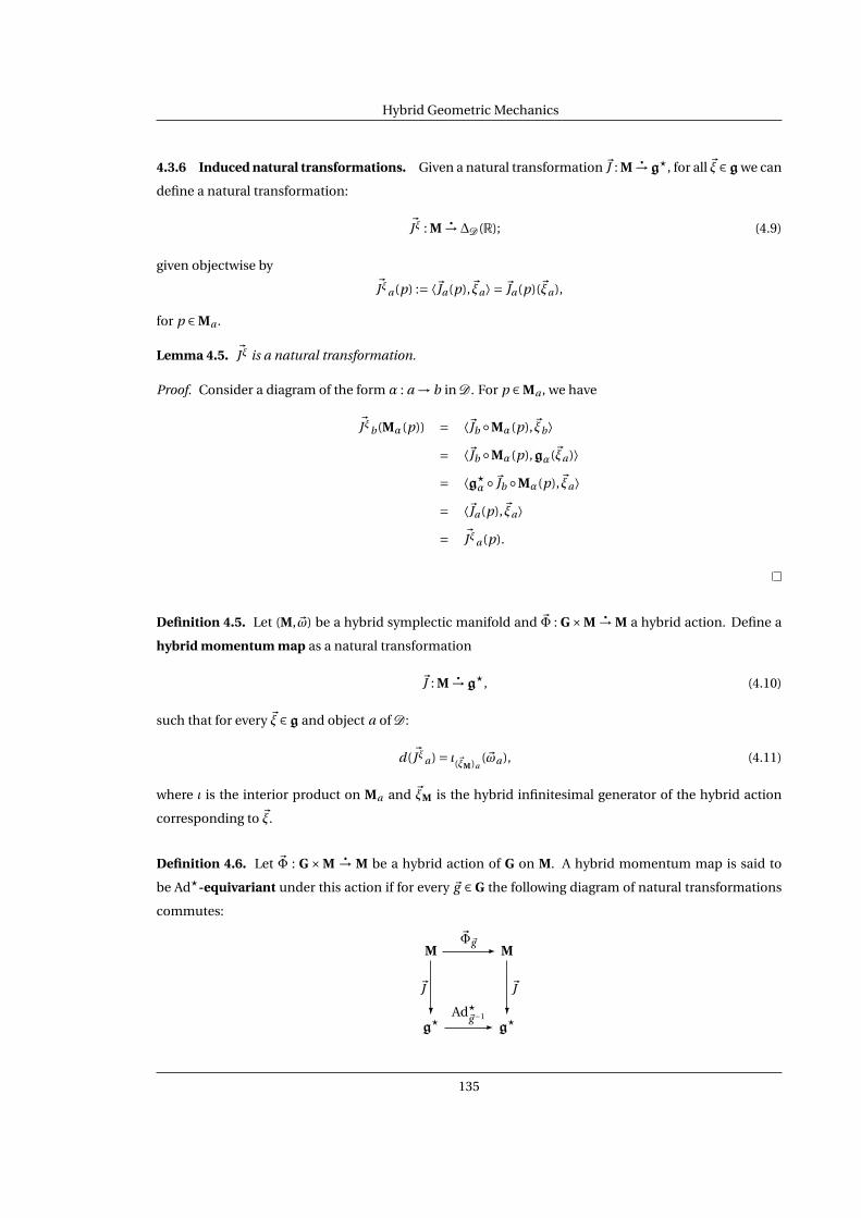
Hybrid Geometric Mechanics
4.3.6 Induced natural transformations. Given a natural transformation ~J : M→g?, for all ~ξ ∈g we can
define a natural transformation:
~Jξ : M→∆D(R); (4.9)
given objectwise by~Jξa(p) := ⟨~Ja(p),~ξa⟩ = ~Ja(p)(~ξa),
for p ∈ Ma .
Lemma 4.5. ~Jξ is a natural transformation.
Proof. Consider a diagram of the form α : a → b in D. For p ∈ Ma , we have
~Jξb(Mα(p)) = ⟨~Jb Mα(p),~ξb⟩= ⟨~Jb Mα(p),gα(~ξa)⟩= ⟨g?
α ~Jb Mα(p),~ξa⟩= ⟨~Ja(p),~ξa⟩= ~Jξa(p).
Definition 4.5. Let (M,~ω) be a hybrid symplectic manifold and ~Φ : G×M→ M a hybrid action. Define a
hybrid momentum map as a natural transformation
~J : M→g?, (4.10)
such that for every ~ξ ∈g and object a of D:
d(~Jξa) = ι(~ξM)a(~ωa), (4.11)
where ι is the interior product on Ma and ~ξM is the hybrid infinitesimal generator of the hybrid action
corresponding to ~ξ.
Definition 4.6. Let ~Φ : G×M→ M be a hybrid action of G on M. A hybrid momentum map is said to
be Ad?-equivariant under this action if for every ~g ∈ G the following diagram of natural transformations
commutes:
M~Φ~g - M
g?
~J
? Ad?~g−1
- g?
~J
?
135

Hybrid Geometric Mechanics
4.3.7 The reduced hybrid phase space. Suppose that G acts on M through the hybrid action ~Φ, and let
~J : M→g? be an Ad?-equivariant hybrid momentum map. Assume that ~µ ∈g? is a hybrid regular value of
~J ; therefore, J−−−111(((~µµµ))) : D →Man is a hybrid manifold. The restriction of the hybrid action ~Φ~g to J−−−111(((~µµµ))) and
G~µ (also denoted by ~Φ~g ):
~Φ~g : J−−−111(((~µµµ)))→ J−−−111(((~µµµ))), ~g ∈ G~µ, (4.12)
is a hybrid action. In other words, if G acts on M, then G~µ acts on J−−−111(((~µµµ))).
If G~µ acts freely and properly on J−−−111(((~µµµ))), then
M~µ := J−−−111(((~µµµ)))///G~µ : D →Man
is a hybrid manifold, and the canonical hybrid projection
~π~µ : J−−−111(((~µµµ)))→ M~µ = J−−−111(((~µµµ)))///G~µ
is a hybrid submersion. M~µ is called the reduced hybrid phase space. In particular, for every α : a → b in
D, there is a commuting diagram
MaMα - Mb
J−−−111(((~µµµ)))a
(~i~µ)a
∪
6
J−−−111(((~µµµ)))α - J−−−111(((~µµµ)))b
(~i~µ)b
∪
6
(M~µ)a = (J−−−111(((~µµµ)))///G~µ)a
(~π~µ)a
? (M~µ)α = (J−−−111(((~µµµ)))///G~µ)α- (M~µ)b = (J−−−111(((~µµµ)))///G~µ)b
(~π~µ)b
?
(4.13)
in Man.
Example 4.3. For our running example of a two-dimensional bouncing ball, we define a hybrid group
action by translating in the x-direction on all domains, i.e., define
~Φball : Gball ×Mball → Gball
by
~Φballb (a, (x, y, px , py )) =
x +a
y
px
py
~Φball
s (b, (x, px )) = x +b
px
~Φball
ab= ~Φball
b |Mballab
~Φballas
= ~Φballb |Mball
as.
136

Hybrid Geometric Mechanics
Using the canonical construction of momentum maps on cotangent bundles, the hybrid momentum map
~J ball : Mball → (gball)? =∆opM ball (R) is given by:
~J ballb (x, y, px , py ) = px ~J ball
s (x, px ) = px
~J ballab
= ~J ballb |Mball
ab
~J ballas
= ~J ballb |Mball
as.
It follows that a hybrid regular value for this system is given by
~µ= (~µb =µ,~µab =µ,~µs =µ,~µas =µ),
for some µ ∈R.
Therefore, the reduced hybrid phase space for the bouncing ball is given by Mball~µ
: M ball →Man,
which is defined by the following diagram: y
py
∈R2 : y = 0 and py ≤ 0
Mball
~µ (M ball) =
R2
ı
?
∩ y
py
7→ y
−epy
? ı ⊃ R0 id - R0
(4.14)
with R0 = 0 a point.
4.4 Hybrid Manifold Reduction
We now introduce the main theorem on reducing a hybrid symplectic manifold. We begin by
reviewing the classic non-hybrid version of this theorem, originally proven by Marsden and Weinstien
[88] (also see [4, 86, 87] for a more thorough account of classical reduction), followed by a statement of the
hybrid version of this theorem.
4.4.1 Classical reduction. The starting point for classical reduction is a Hamiltonian G-space,
(M ,ω,Φ, J),
where
¦ (M ,ω) is a symplectic manifold,
¦ Φ : G ×M → M is a symplectic action of a Lie group on M ,
¦ J is an Ad?-equivariant momentum map for this action.
Under these conditions, the classical reduction theorem [88] reads:
137

Hybrid Geometric Mechanics
Theorem 4.1. Let (M ,ω,Φ, J) be a Hamiltonian G-space and µ ∈ g? be a regular value of J. If the action of
Gµ on J−1(µ) is free and proper, then Mµ = J−1(µ)/Gµ has a unique symplectic form ωµ with the property:
Ω2(πµ)(ωµ) =Ω2(iµ)(ω),
where πµ : J−1(µ) → Mµ is the canonical projection and iµ : J−1(µ) → M is the inclusion.
The hybrid reduction theorem will nicely mirror and utilize this theorem. There also is an in-
triguing connection between the classical reduction theorem and hybrid symplectic manifolds; this the-
orem implies that the following hybrid manifold
M iµ ⊃ J−1(µ)
πµ- Mµ
is a hybrid symplectic manifold.
4.4.2 Hybrid Hamiltonian G-spaces. Utilizing the framework developed thus far, we can prove a hy-
brid version of Theorem 4.1. First, we note that the necessary information in order to generalize this
theorem is a hybrid Hamiltonian G-space, i.e., a tuple
(M,~ω,~Φ,~J),
where
¦ (M,~ω) is a hybrid symplectic manifold,
¦ ~Φ : G×M→ M is a symplectic hybrid action of a Lie group on M,
¦ ~J is an Ad?-equivariant hybrid momentum map for this hybrid action.
For such a hybrid Hamiltonian G-space, we can reduce the dimensionality of M through hybrid reduction.
This is done by utilizing the classical reduction theorem through the observation that
(Mb ,~ωb ,~Φb ,~Jb)
is a Hamiltonian Gb-space for every b ∈V(D).
Before stating the theorem, recall that for a morphism of hybrid manifolds ~f : M→ N,
Ω2∗(~f ) : Ω2
∗(N)→Ω2
∗(M),
which is the natural transformation obtained from applying the functor Hy(Ω2) (see Paragraph 4.1.4).
Theorem 4.2. Let (M,~ω,~Φ,~J) be a hybrid Hamiltonian G-space. Assume ~µ ∈g? is a hybrid regular value of
~J and that the hybrid action of G~µ on J−−−111(((~µµµ))) is free and proper. Then M~µ has a unique hybrid symplectic
form ~ω~µ with the property:
Ω2∗(~π~µ)(~ω~µ) =Ω2
∗(~i~µ)(~ω).
138

Hybrid Geometric Mechanics
Proof. The goal is to define a hybrid symplectic form ~ω~µ on M~µ. To do so, we first note that it follows from
the definition of (M,~ω,~Φ,~J) that, for all b ∈V(D),
(Mb ,~ωb ,~Φb ,~Jb)
is a Hamiltonian Gb-space, ~µb is a regular value of ~Jb , and the action of (G~µ)b on J−−−111(((~µµµ)))b is free and proper.
Therefore, for b ∈V(D), define (~ω~µ)b to be the unique symplectic form satisfying:
Ω2∗(~π~µ)b((~ω~µ)b) =Ω2
∗(~i~µ)b(~ωb).
For a ∈E(D) there is a diagram of the form
cod(sa) sa ata- cod(ta) (4.15)
in D. To complete the description of ~ω~µ, define (~ω~µ)a by the requirement that
Ω2∗(M~µ)sa ((~ω~µ)cod(sa )) = (~ω~µ)a =Ω2
∗(M~µ)ta ((~ω~µ)cod(ta )).
To complete the proof, we must show that ~ω~µ is well-defined and unique. Uniqueness clearly
follows from the uniqueness of (~ω~µ)cod(sa ) and (~ω~µ)cod(ta ) and the definition of a hybrid symplectic form.
Therefore, we must only show that it is well-defined, i.e., that
Ω2∗(M~µ)sa ((~ω~µ)cod(sa )) =Ω2
∗(M~µ)ta ((~ω~µ)cod(ta ))
for all a ∈E(D).
For the diagram (4.15) in D, because the diagram in (4.13) commutes, we have that the diagram:
Mcod(sa ) Msa Ma
Mta - Mcod(ta )
J−−−111(((~µµµ)))cod(sa )
(~i~µ)cod(sa )
∪
6
J−−−111(((~µµµ)))sa J−−−111(((~µµµ)))a
(~i~µ)a
∪
6
J−−−111(((~µµµ)))ta - J−−−111(((~µµµ)))cod(ta )
(~i~µ)cod(ta )
∪
6
(M~µ)cod(sa )
(~π~µ)cod(sa )
?
(M~µ)sa(M~µ)a
(~π~µ)a
? (M~µ)ta - (M~µ)cod(ta )
(~π~µ)cod(ta )
?
139
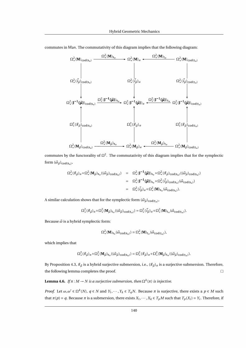
Hybrid Geometric Mechanics
commutes in Man. The commutativity of this diagram implies that the following diagram:
Ω2∗(M)cod(sa )
Ω2∗(M)sa - Ω2∗(M)a
Ω2∗(M)taΩ2
∗(M)cod(ta )
Ω2∗(J−−−111(((~µµµ))))cod(sa )
Ω2∗(~i~µ)cod(sa )
?Ω2∗(J−−−111(((~µµµ))))sa- Ω2
∗(J−−−111(((~µµµ))))a
Ω2∗(~i~µ)a
?Ω
2∗(J−−−111(((~µµµ))))taΩ2
∗(J−−−111(((~µµµ))))cod(ta )
Ω2∗(~i~µ)cod(ta )
?
Ω2∗(M~µ)cod(sa )
Ω2∗(~π~µ)cod(sa )
6
Ω2∗(M~µ)sa - Ω2∗(M~µ)a
Ω2∗(~π~µ)a
6
Ω2∗(M~µ)ta
Ω2∗(M~µ)cod(ta )
Ω2∗(~π~µ)cod(ta )
6
commutes by the functorality of Ω2. The commutativity of this diagram implies that for the symplectic
form (~ω~µ)cod(sa ),
Ω2∗(~π~µ)a Ω2
∗(M~µ)sa ((~ω~µ)cod(sa )) = Ω2∗(J−−−111(((~µµµ))))sa Ω2
∗(~π~µ)cod(sa )((~ω~µ)cod(sa ))
= Ω2∗(J−−−111(((~µµµ))))sa Ω2
∗(~i~µ)cod(sa )(~ωcod(sa ))
= Ω2∗(~i~µ)a Ω2
∗(M)sa (~ωcod(sa )).
A similar calculation shows that for the symplectic form (~ω~µ)cod(ta ),
Ω2∗(~π~µ)a Ω2
∗(M~µ)ta ((~ω~µ)cod(ta )) =Ω2∗(~i~µ)a Ω2
∗(M)ta (~ωcod(ta )).
Because ~ω is a hybrid symplectic form:
Ω2∗(M)sa (~ωcod(sa )) =Ω2
∗(M)ta (~ωcod(ta )),
which implies that
Ω2∗(~π~µ)a Ω2
∗(M~µ)sa ((~ω~µ)cod(sa )) =Ω2∗(~π~µ)a Ω2
∗(M~µ)ta ((~ω~µ)cod(ta )).
By Proposition 4.3, ~π~µ is a hybrid surjective submersion, i.e., (~π~µ)a is a surjective submersion. Therefore,
the following lemma completes the proof.
Lemma 4.6. If π : M → N is a surjective submersion, then Ωk (π) is injective.
Proof. Let ω,ω′ ∈ Ωk (N), q ∈ N and Y1, · · · ,Yk ∈ Tq N . Because π is surjective, there exists a p ∈ M such
that π(p) = q. Because π is a submersion, there exists X1, · · · ,Xk ∈ TpM such that Tp(Xi ) = Yi . Therefore, if
140

Hybrid Geometric Mechanics
Ωk (π)(ω) =Ωk (π)(ω′),
ωq (Y1, · · · ,Yn) = Ωk (π)(ω)p(X1, · · · ,Xk )
= Ωk (π)(ω′)p(X1, · · · ,Xk )
= ω′q (Y1, · · · ,Yn)
as desired.
4.5 Hybrid Hamiltonian Reduction
The hybrid reduction theorem (Theorem 4.2) only gave conditions on when the phase space of a
hybrid system can be reduced. In practice, we are interested in reducing the dynamics of a hybrid system.
That is, we want to understand how to reduce hybrid Hamiltonians. This yields a method for reducing
hybrid systems.
4.5.1 Classical Hamiltonian reduction. Before discussing how to reduce hybrid Hamiltonians, and
hence hybrid systems obtained from hybrid Hamiltonians, we review the classical Hamiltonian reduc-
tion theorem (cf. [4]). The setup for this theorem is a Hamiltonian G-space (M ,ω,Φ, J) satisfying the
assumptions given in Theorem 4.1.
A Hamiltonian system is a tuple (M ,ω,H), where (M ,ω) is a symplectic manifold and H : M →R
is a Hamiltonian. From the Hamiltonian H , we obtain a vector field XH defined by d(H) = ιXH (ω). That is,
associated to the Hamiltonian system (M ,ω,H) there is a dynamical system (M ,XH ), or an object of Dyn.
Recall (see Definition 2.4) that a trajectory of (M ,XH ) is an object (I ,d/dt) of Interval(Dyn) together with a
morphism of dynamical systems:
c : (I ,d/dt) → (M ,XH ).
In other words c(t ) = XH (c(t )). The initial condition of such a trajectory is c(t0).
A Hamiltonian H : M →R is said to be G-invariant if for the action Φ : G ×M → M ,
H Φ(g , − ) = H .
for all g ∈G . From a G-invariant Hamiltonian, we obtain a Hamiltonian Hµ on Mµ defined by the require-
ment that it make the following diagram
J−1(µ)iµ - M
Mµ
πµ
? Hµ - R
H
?
commute. The end result is reduced Hamiltonian system (Mµ,ωµ,Hµ), for which we have an associated
dynamical system (Mµ,XHµ ). We denote trajectories of this dynamical system by
cµ : (I ,d/dt) → (Mµ,XHµ ).
141

Hybrid Geometric Mechanics
The classical Hamiltonian reduction theorem (cf. [4] and [88]) relates trajectories of (M ,XH ) and
trajectories of (Mµ,XHµ ). We state this result in a slightly different formulism, although it is equivalent to
the standard result.
Theorem 4.3. Let (M ,ω,Φ, J) be a Hamiltonian G-space satisfying the assumptions given in Theorem 4.1.
If H is a G-invariant Hamiltonian and c : (I ,d/dt) → (M ,XH ) is a trajectory of (M ,XH ) with c(t0) ∈ J−1(µ),
then
c : (I ,d/dt) → (J−1(µ),XH )
and there exists a trajectory cµ : (I ,d/dt) → (Mµ,XHµ ) of (Mµ,XHµ ) defined by the factorization:
(I ,d/dt)cµ - (Mµ,XHµ )
(J−1(µ),XH )
πµ
-
c -
Remark 4.2. In Theorem 4.3, it would have been more accurate to write (J−1(µ),XH |J−1(µ)) instead of
(J−1(µ),XH ). We opted for the latter notation as it is clear from context that, in this case, XH must be
restricted to take values in J−1(µ).
We now establish the necessary groundwork needed in order to establish the hybrid analogue
of Theorem 4.3. We begin by defining hybrid Hamiltonians. In doing so, we again make explicit the D-
category associated with hybrid objects, e.g., we will now denote the hybrid manifold M by (M ,M). The
motivation for this is that we are once again interested in trajectories.
Definition 4.7. A hybrid Hamiltonian H on a hybrid manifold (M ,M) is defined to be a set of maps:
H = Hq : Mq →Rq∈V(M ).
A hybrid Hamiltonian system is a tuple (M ,M,~ω,H), where (M ,M,~ω) is a hybrid symplectic manifold and
H is a hybrid Hamiltonian.
Example 4.4. For the bouncing ball hybrid manifold (M ball,Mball), consider the hybrid Hamiltonian
Hball = Hballb ,Hball
s ,
where
Hballb (x, y, px , py ) = 1
2m(p2
x +p2y )+mg y,
Hballs (x, px ) = 1
2mp2
x .
The bouncing ball hybrid Hamiltonian system is given by
(M ball,Mball,~ωball,Hball),
where ~ωball is the hybrid symplectic form given in Example 4.1.
142

Hybrid Geometric Mechanics
4.5.2 G-Invariant hybrid Hamiltonians. Let (M ,G) be a hybrid Lie group acting on the hybrid mani-
fold (M ,M) through the hybrid action:
(~IdM ,~Φ) : (M ,G×M) → (M ,M).
A hybrid Hamiltonian H is said to be G-invariant if
Hq ~Φq (g ,−) = Hq
for all g ∈ Gq and q ∈V(M ), i.e., Hq is Gq -invariant for all q ∈V(M ).
Under the assumptions of Theorem 4.2, if H is a G-invariant hybrid Hamiltonian on (M ,M),
then there is a hybrid Hamiltonian
H~µ = (H~µ)q : (M~µ)q →Rq∈V(M )
on M~µ defined by requiring that the following diagram commute:
J−−−111(((~µµµ)))q(~i~µ)q- Mq
(M~µ)q
(~π~µ)q
? (H~µ)q- R
Hq
?
for all q ∈V(M ). This defines a hybrid Hamiltonian system (M ,M~µ,~ω~µ,H~µ).
4.5.3 Trajectories of hybrid Hamiltonian systems. From a hybrid Hamiltonian system (M ,M,~ω,H)
we obtain a (categorical) hybrid system:
(M ,M,XH),
where XH is the collection of vector fields given by XH = (XH)q q∈V(M ), with (XH)q defined by the require-
ment that
d(Hq ) = ι(XH)q (~ωq ).
Similarly, we obtain a hybrid system (M ,M~µ,XH~µ) from the hybrid Hamiltonian system (M ,M~µ,~ω~µ,H~µ).
Note that (M ,M,XH) and (M ,M~µ,XH~µ) do not correspond to “classical” hybrid systems unless
we make certain assumptions on the hybrid manifold (M ,M), i.e., that it is of the form (M ,Mııı ) (see Para-
graph 2.1.2, Proposition 2.1 and Proposition 2.2).
Recall from Definition 2.7 that a trajectory of the hybrid system (M ,M,XH) consists of an object
(I ,I,d///dt) of Interval(HySys) together with a morphism of hybrid systems:
(~C ,~c) : (I ,I,d///dt) → (M ,M,XH).
The initial condition of such a trajectory is (~C (0),~c0(τ0)) with ~c0(τ0) ∈ M~C (0).
143

Hybrid Geometric Mechanics
Example 4.5. For the bouncing ball, the reduced hybrid Hamiltonian is given by:
Hball~µ = (Hball
~µ )b , (Hball~µ )s ,
where
(Hball~µ )b(y, py ) = 1
2mp2
y +mg y + 1
2mµ2,
(Hball~µ )s (0) = 1
2mµ2.
From this we obtain the reduced hybrid Hamiltonian system:
(M ball,Mball~µ ,~ωball
~µ ,Hball~µ ),
where ~ωball~µ
is the “canonical” symplectic form on the reduced phase space (M ,Mball~µ
). From the reduced
hybrid Hamiltonian system, we obtain the reduced hybrid system:
(M ball,Mball~µ ,Xball
~µ ),
where Mball~µ
is defined as in (4.14) and
Xball~µ = (Xball
~µ )b , (Xball~µ )s
with
(Xball~µ )b(y, py ) = 1
m
py
−m2g
,
(Xball~µ )s (0) = 0.
Therefore, the reduced hybrid system is exactly the hybrid system modeling a one-dimensional bouncing
ball which stops bouncing once the Zeno point is reached.
We now demonstrate that the “dynamics” of H determine the corresponding “dynamics” of H~µ
in the hybrid analogue to Theorem 4.3.
Theorem 4.4. Let (M,~ω,~Φ,~J) be a hybrid Hamiltonian G-space satisfying the assumptions of Theorem 4.2.
If H is a G-invariant Hamiltonian and (~C ,~c) : (I ,I,d///dt) → (M ,M,XH) is a trajectory of (M ,M,XH) with
~c0(τ0) ∈ J−−−111(((~µµµ)))~C (0), then
(~C ,~c) : (I ,I,d///dt) → (M ,J−−−111(((~µµµ))),XH)
and there exists a trajectory (~C ,~c~µ) : (I ,I,d///dt) → (M ,M~µ,XH~µ) of (M ,M~µ,XH~µ
) defined by the factoriza-
tion:
(I ,I,d///dt)(~C ,~c~µ)
- (M ,M~µ,XH~µ)
(M ,J−−−111(((~µµµ))),XH)
(~IdM ,~π~µ)
-
(~C ,~c) -
144

Hybrid Geometric Mechanics
Proof. We must first show that for a trajectory
(~C ,~c) : (I ,I,d///dt) → (M ,M,XH)
of (M ,M,XH),
~c(τ0) ∈ J−−−111(((~µµµ)))~C (0) ⇒ (~C ,~c) : (I ,I,d///dt) → (M ,J−−−111(((~µµµ))),XH).
It is enough to show that
~c0(τ0) ∈ J−−−111(((~µµµ)))~C (0) ⇒ (~C ,~c) : (I ,I) → (M ,J−−−111(((~µµµ)))). (4.16)
This would imply that ~ci (τi ) ∈ J−−−111(((~µµµ)))~C (i ) and by Theorem 4.3 we know that
~ci (τi ) ∈ J−−−111(((~µµµ)))~C (i ) ⇒ ~ci : (Ii ,d/dt) → (J−−−111(((~µµµ)))~C (i ), (XH)~C (i ))
for all i ∈V(I ).
To show (4.16), it is clearly sufficient to show:
~ci−1(τi−1) ∈ J−−−111(((~µµµ)))~C (i−1) ⇒ ~ci (τi ) ∈ J−−−111(((~µµµ)))~C (i ), (4.17)
for i − 1, i ∈ V(I ); (4.16) would then follow from Theorem 4.3. Assuming that ~ci−1(τi−1) ∈ J−−−111(((~µµµ)))~C (i−1)
(hence, assuming that ~ci−1(t ) ∈ J−−−111(((~µµµ)))~C (i−1) for all t ∈ Ii−1), we need to show that for every diagram of the
form
i −1 sei ei = (i −1, i )
tei - i
in I ,
~J~C (i−1)(~ci−1(τi )) = ~µ~C (i−1) ⇒ ~J~C (ei )(~cei (τi )) = ~µ~C (ei ) (4.18)
⇒ ~J~C (i )(~ci (τi )) = ~µ~C (i ).
First note that because ~c is a natural transformation, the diagram
Ii−1
Isei= ι
⊃ Iei⊂
Itei= ι
- Ii
M~C (i−1)
~ci−1
?M~C (sei )
M~C (ei )
~cei
? M~C (tei )- M~C (i )
~ci
?
commutes.
Since ~µ ∈ g?, we know that g?~C (sei )
(~µ~C (i−1)) = ~µ~C (ei ). By the naturality of ~J , i.e., because of the
commuting diagram given in (4.6),
~J~C (ei )(~cei (τi )) = g?~C (sei )
(J~C (i−1)(M~C (sei )(~cei (τi ))))
= g?~C (sei )
(J~C (i−1)(~ci−1(τi )))
= g?~C (sei )
(~µ~C (i−1))
= ~µ~C (ei ).
145

Hybrid Geometric Mechanics
Since we are assuming that ~µ is a hybrid regular value of ~J (Definition 4.4), we have that:
~J~C (ei )(~cei (τi )) = ~µ~C (ei ) ⇒ ~µ~C (i ) = ~J~C (i )(M~C (tei )(~cei (τi ))) = ~J~C (i )(~ci (τi )).
Therefore, (4.18) coupled with the naturality of ~c implies (4.17), which in turn implies (4.16).
Now, we need to show that
(~IdM ,~π~µ) : (M ,J−−−111(((~µµµ))),XH) → (M ,M~µ,XH~µ)
is a morphism of hybrid systems. Theorem 4.2 implies that
(~IdM ,~π~µ) : (M ,J−−−111(((~µµµ)))) → (M ,M~µ)
is a morphism of hybrid manifolds, so we need only show that
(~π~µ)b : (J−−−111(((~µµµ)))b , (XH)b) → ((M~µ)b , (XH~µ)b)
is a morphism of dynamical systems for all b ∈V(M ), but this follows from Theorem 4.3.
Finally, it follows from Lemma 2.1 that
(~C ,~c~µ) := (~IdM ,~π~µ) (~C ,~c) : (I ,I,d///dt) → (M ,M~µ,XH~µ)
is a trajectory of (M ,M~µ,XH~µ).
146

Chapter 5
Zeno Behavior & Hybrid Stability Theory
Zeno behavior is a phenomena that is unique to hybrid systems; it has no counterpart in dis-
crete or continuous systems. It has remained relatively unexplored over the years—before the work of the
author [18] there were no sufficient conditions for the existence of Zeno behavior in general hybrid sys-
tems. This is a byproduct of the fact that to determine whether Zeno behavior exists in a hybrid system,
the vector fields on each domain must be solved for explicitly. Since this generally is not possible, finding
sufficient conditions on the existence of Zeno has remained an open problem in the hybrid systems com-
munity, at least in the case when the vector fields on each domain are nontrivial, i.e., when they are not
constant vector fields.
It is only through a necessary paradigm shift in the study of hybrid stability that we are able to
provide a remedy. It is only through the use of categories of hybrid objects that we are able to provide
sufficient conditions for a general class of hybrid systems.
Zeno behavior can be likened to stability, in that its existence implies a type of convergence; the
convergence is to a set, termed a Zeno equilibria, that is invariant under the discrete dynamics. Super-
ficially, this is where the similarities end, e.g., each element of the Zeno equilbria set cannot be a zero of
its corresponding vector field. Motivated by the peculiarities of Zeno equilibria, we consider a form of
asymptotic stability that is global in the continuous state, but local in the discrete state. We provide suffi-
cient conditions for stability of these equilibria, resulting in sufficient conditions for the existence of Zeno
behavior.
Regardless of, or because of, the unique nature of Zeno equilibria, they can arise in many sys-
tems of interest, e.g., mechanical systems undergoing impacts. The convergent behavior of these systems
is often of interest—even if this convergence is not to “classical” notions of equilibrium points. This mo-
tivates the study of Zeno equilibria because even if the convergence is not classical, it still is important.
For example, simulating trajectories of these systems is an important component in their analysis, yet this
may not be possible due to the relationship between Zeno equilibria and Zeno behavior.
An equally important reason to address the stability of Zeno equilibria is to be able to assess the
147

Zeno Behavior & Hybrid Stability Theory
existence of Zeno trajectories. This behavior is infamous in the hybrid system community for its ability to
halt simulations. The only way to prevent this undesirable outcome is to give a priori conditions on the ex-
istence of Zeno behavior. This has motivated a profuse study of Zeno hybrid systems (see [33, 59, 69, 119]
to name a few) but a concrete notion of convergence (in the sense of stability) has not yet been introduced.
As a result, there is a noticeable lack of sufficient conditions for the existence of Zeno behavior.
The main contribution of this chapter is sufficient conditions for the stability of Zeno equilibria.
As a byproduct, we are able to give sufficient conditions for the existence of Zeno behavior. The categori-
cal approach to hybrid systems allows us to decompose the study of stability into two manageable steps.
The first step consists of identifying a sufficiently rich, yet sufficiently simple, class of hybrid systems em-
bodying the desired stability properties: first quadrant hybrid systems. The second step is to understand
the stability of general hybrid systems by understanding the relationships between these systems and first
quadrant hybrid systems described by morphisms (in the category of hybrid systems).
In this vain, we devote some effort to the introduction of first quadrant hybrid systems, demon-
strating in a step-by-step fashion how to transform these systems into categorical hybrid systems. We
then study a special class of first quadrant hybrid systems, diagonal first quadrant hybrid systems, giving
sufficient conditions for the existence of Zeno behavior in systems of this form. The techniques employed,
while not immediately generalizable, indicate a fundamental connection between stability and Zeno. We
then proceed to study general hybrid systems, and Zeno equilibria, through the use of categories of hybrid
objects and thus solidify the connection between stability and Zeno behavior. We conclude the chapter
by indicating how it is possible to “go beyond” Zeno, i.e., carry trajectories past a Zeno point, in a simple
class of hybrid systems: Lagrangian hybrid systems.
Related work. There has been a rather profuse study of Zeno equilibria (see [48, 59, 68, 69, 103, 104, 118,
119], to name a few), yet a concrete notion of convergence (in the sense of stability) has not been formally
introduced (except in [18], on which this chapter is based). The author has explored this relationship in
some limited contexts, namely in [7] where diagonal first quadrant hybrid systems were studied, and [12]
where the geometric “stability preserving” regularization of a class of hybrid systems was considered; in
fact, the latter paper first introduces the notion of a Zeno equilibria, albeit a special case thereof. In addi-
tion, the author has studied the relationship between Zeno behavior and the topology of hybrid systems
in [13] and [14]. Finally, methods for carrying executions past the point(s) at which Zeno behavior occurs
has been studied in [19] and [121].
While the convergent properties of Zeno equilibria have not been well-studied, the stability of
hybrid and switched systems has. We refer the reader to [32, 33, 34, 35, 52, 80, 81, 94, 120] for some of the
approaches taken. While our approach is essentially different, there are analogies that can be drawn. For
example, common to the study of stability of hybrid systems is the idea of multiple Lyapunov functions
[34]. In fact, we arrive at a similar construction in Theorem 5.5, where the morphism between hybrid
systems can be viewed as a “hybrid Lyapunov function” and, as such, consists of a collection of Lyapunov
functions.
148
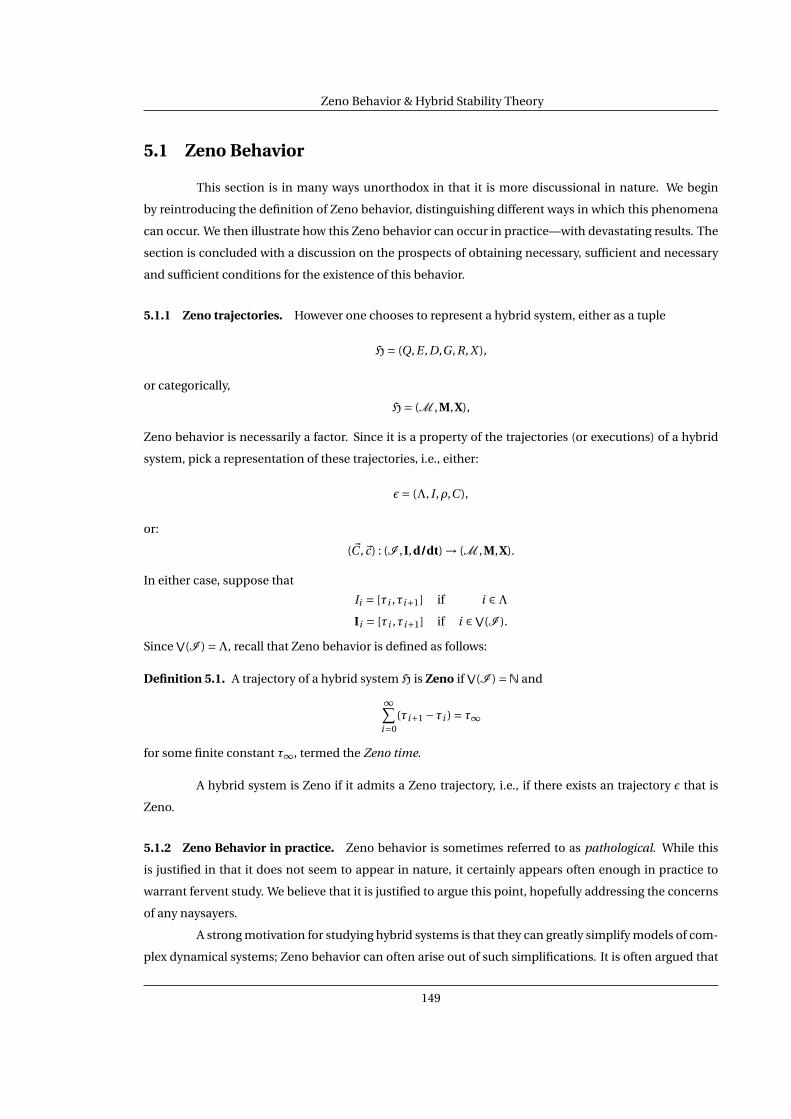
Zeno Behavior & Hybrid Stability Theory
5.1 Zeno Behavior
This section is in many ways unorthodox in that it is more discussional in nature. We begin
by reintroducing the definition of Zeno behavior, distinguishing different ways in which this phenomena
can occur. We then illustrate how this Zeno behavior can occur in practice—with devastating results. The
section is concluded with a discussion on the prospects of obtaining necessary, sufficient and necessary
and sufficient conditions for the existence of this behavior.
5.1.1 Zeno trajectories. However one chooses to represent a hybrid system, either as a tuple
H= (Q,E ,D,G ,R,X ),
or categorically,
H= (M ,M,X),
Zeno behavior is necessarily a factor. Since it is a property of the trajectories (or executions) of a hybrid
system, pick a representation of these trajectories, i.e., either:
ε= (Λ, I ,ρ,C ),
or:
(~C ,~c) : (I ,I,d///dt) → (M ,M,X).
In either case, suppose that
Ii = [τi ,τi+1] if i ∈Λ
Ii = [τi ,τi+1] if i ∈V(I ).
Since V(I ) =Λ, recall that Zeno behavior is defined as follows:
Definition 5.1. A trajectory of a hybrid system H is Zeno if V(I ) =N and
∞∑i=0
(τi+1 −τi ) = τ∞
for some finite constant τ∞, termed the Zeno time.
A hybrid system is Zeno if it admits a Zeno trajectory, i.e., if there exists an trajectory ε that is
Zeno.
5.1.2 Zeno Behavior in practice. Zeno behavior is sometimes referred to as pathological. While this
is justified in that it does not seem to appear in nature, it certainly appears often enough in practice to
warrant fervent study. We believe that it is justified to argue this point, hopefully addressing the concerns
of any naysayers.
A strong motivation for studying hybrid systems is that they can greatly simplify models of com-
plex dynamical systems; Zeno behavior can often arise out of such simplifications. It is often argued that
149

Zeno Behavior & Hybrid Stability Theory
Figure 5.1: Zeno behavior that effectively makes a program (Matlab) halt.
if Zeno arises is such a case, the model is wrong—maybe a hybrid model is not the right one. Rather than
“throwing the baby out with the bath water,” the author believes that it is better to understand the role of
Zeno behavior in hybrid systems in order to more effectively deal with the phenomena. To those who are
not in agreement, a simpler rebuttal is: in order to modify Zeno models so that they are no longer Zeno,
one must first detect that they are Zeno. Hence we are back to our initial claim: Zeno behavior needs to be
properly understood.
One may now argue that Zeno behavior does not appear often enough to be an interesting phe-
nomena. Yet, as was seen in Chapter 3, mechanical systems undergoing impacts are naturally modeled
as hybrid systems; if systems of this form loose energy at each impact, they will tend to display Zeno
behavior. If the category of all mechanical systems undergoing impacts does not provide a large enough
example of systems that can display Zeno behavior, one can rest assured that there are more. For example,
hybrid models of communication networks display Zeno behavior (cf. Figure 5.2), as illustrated in [2].
After hopefully convincing the reader as to the necessity of studying Zeno behavior, it is impor-
tant to remark on how it manifests itself. To provide a quintessential example, if one runs the bouncing
ball example in Matlab’s Simulink for 25 seconds (rather then the default 20 seconds) the simulation will
never finish; see Figure 5.1. Zeno behavior makes a simulator effectively halt. This implies that the ex-
istence of such behavior can have catastrophic effects on the simulation—hence verification—of hybrid
systems. If it were possible to detect the existence or non-existence of this behavior a priori, it could have
far-reaching effects.
5.1.3 Types of Zeno. The definition of a Zeno trajectory results in two qualitatively different types of
Zeno behavior (as first introduced in [13]); they are defined as follows: a Zeno trajectory is
Chattering Zeno: If there exists a finite C such that
τi+1 −τi = 0
for all i ≥C .Genuinely Zeno: If
τi+1 −τi > 0
for all i ∈N.
150

Zeno Behavior & Hybrid Stability Theory
0 5 10 15 20 25 30 35 40 450
5
10
15
20
25
30
35
40
45
0 5 10 15 20 25 300
5
10
15
20
25
30
Figure 5.2: An example of Genuine Zeno behavior (left). An example of Chattering Zeno behavior (right).
There are obviously more characterizations of Zeno behavior—ones that could go beyond simple condi-
tions on the differences between successive switching times. This will be discussed in more detail after
we illustrate the differences between chattering and genuine Zeno behavior, which is especially prevalent
in there detection and elimination.
Chattering Zeno trajectories (cf. Figure 5.2) result from the existence of a switching surface on
which the vector fields “oppose” each other; for this reason they are easy to detect (simply look at the
orientation of the vector fields along the guards). In addition, they can be eliminated in a fairly simple
manner. Filippov solutions can be defined on these surfaces in order to force the flow to “slide” along the
switching surface [50]. Later in this chapter we will generalize this technique to extend genuinely Zeno
executions past the Zeno point.
Genuinely Zeno trajectories (cf. Figure 5.2) are much more complicated in their behavior. The
only methods currently available to detect the existence of trajectories of this form can be found within
this chapter. Very little has been done in the area of eliminating these executions, although there have
been some results [12] and [69], again for a special class of hybrid systems.
To better understand why this is the case, recall that the bouncing ball is, in fact, globally (minus
the origin) genuinely Zeno (if 0 < r < 1), i.e., every trajectory is Zeno. Recall from Example 2.17 that the
the Zeno time for the bouncing ball is given by:
τball∞ =
∞∑i=0
(τballi+1 −τball
i ) =x2 + (1−2g )
√2g x1 +x2
2
g+
∞∑i=0
2
√2g x1 +x2
2
gr i .
For a geometric sequences ar i i∈N, recall that picking initial conditions x1 = a2g /8 and x2 = 0 for a tra-
jectory of the bouncing ball yields:
τball∞ =±
(1
2a(1−2g )+
∞∑i=0
ar i
),
where the expression on the right is positive if a is positive and negative if a is negative. This implies
that even for one of the simplest examples of a hybrid system—the bouncing ball—the switching times
151

Zeno Behavior & Hybrid Stability Theory
effectively yield any geometric series.1
Therefore, to completely characterize the switching times of Zeno trajectories, it is reasonable to
suspect that one would need to effectively characterize all series and the convergence properties thereof.
This is assuming that one were able to solve for the switching times—something that is not even possible
for linear hybrid systems since it involves solving transcendental equations. All of this hints at the com-
plexity of Zeno behavior—determining conditions on the existence or non-existence of Zeno behavior is
a formidable task that will take serious and concerted effort.
5.2 First Quadrant Hybrid Systems
This section is devoted to the study of first quadrant hybrid systems, categorical hybrid systems,
and their interplay. We begin by defining first quadrant hybrid systems; these systems are easy to under-
stand and analyze, but lack generality. Yet, they are very useful for understanding Zeno behavior in general
hybrid systems. The connection between these two types of systems—first quadrant hybrid systems and
general hybrid systems—is achieved through the use of morphisms of hybrid systems. Therefore, we be-
gin by introducing first quadrant hybrid systems using the classical notation for hybrid systems. We then
proceed to demonstrate, in a step-by-step fashion, how to obtain a categorical representation of these
systems.
5.2.1 First quadrant hybrid systems. First quadrant hybrid systems are hybrid systems which can be
viewed as the “simplest” hybrid systems that display Zeno behavior.
A first quadrant hybrid system, or just FQ hybrid system, is a tuple:
HFQ = (Γ,D,G ,R,X ),
where
¦ Γ= (Q,E) is a directed cycle, with
Q = 1, . . . , k, E = e1 = (1,2), e2 = (2,3), . . . , ek = (k,1).
¦ D = Di i∈Q , where for all i ∈Q,
Di = (R+0 )2 =
x1
x2
∈R2 : x1 ≥ 0 and x2 ≥ 0
,
hence the name “first quadrant.”
¦ G = Ge e∈E , where for all e ∈ E
Ge =
x1
x2
∈R2 : x1 = 0 and x2 ≥ 0
.
1As a side note, our proof later in this chapter that the bouncing ball is Zeno does not rely on the convergence of geometric series,and so we prove, independently, that geometric series converge (when 0 ≤ r < 1).
152

Zeno Behavior & Hybrid Stability Theory
D1Re1Re2Ge1 Ge2
Dball2Dball
1
Gballe1 Gballe2
Rballe1
Rballe2
Figure 5.3: The hybrid system HballFQ .
¦ R = Re e∈E , where Re : Ge → (R+0 )2 and for all e ∈ E there exists a function re :R+
0 →R+0 with
Re (x1, x2) = re (x2)
x1
.
¦ X = Xi i∈Q , where Xi is a Lipshitz vector field on (R+0 )2.
Remark 5.1. We could consider higher dimensional FQ hybrid systems, but this would add complication
without generality.
Example 5.1. We will transform the bouncing ball hybrid system introduced in Example 2.1 into a first
quadrant hybrid system:
HballFQ = (Γball,Dball,Gball,Rball,X ball)
by dividing the original domain into two components, and changing the vector fields accordingly.
We first define Γball to be the directed cycle:
1e1 -e2
2
Since HballFQ will be a first quadrant hybrid system, the domains and guards must satisfy the conditions
given in Paragraph 5.2.1. In the case of the bouncing ball, the domain Dball1 is obtained from the top half
of the original domain for the bouncing ball by reflecting it around the line x1 = x2. The domain Dball2 is
obtained from the bottom half of the original domain by reflecting it around the line x2 = 0. This implies
153

Zeno Behavior & Hybrid Stability Theory
that the reset maps are given by2
Rballe1
(x1, x2) = x2
x1
, Rballe2
(x1, x2) = ex2
x1
.
Finally, the transformed vector fields are given by
X ball1 (x1, x2) =
−g
x1
, X ball2 (x1, x2) =
−x2
g
.
A graphical representation of this system can be seen in Figure 5.3.
5.2.2 Categorical FQ hybrid systems. We now proceed to show, in a step-by-step fashion, how to ob-
tain a categorical FQ hybrid system (M FQ,MFQ,XFQ) from a first quadrant hybrid system HFQ.
The graph for a FQ hybrid system is given by a directed k-cycle graph:
1e1- 2
k
ek-3
e2-
......
i +2 i −1
i +1 ei
ei+1
i
ei−1
Therefore, the associated D-category, M FQ, is given by:
M FQ =
e1
ek e2
1
se1
tek
-2
te1
- se2
k
sek -
3
te2
......
i +2 i −1
i +1 i
ei+1
tei+1
-
sei+1
-
ei−1
sei−1
tei−1
ei
sei
-
tei
The hybrid space of HFQ is the tuple (Γ,D,G ,R). Therefore, as outlined in Proposition 2.1, the
hybrid manifold associated to HFQ is given by the pair (M FQ,MFQ) where MFQ is the functor defined on
2Note that we do not denote the coefficient of restitution for this system by “e” and not “r” due to the notation used to define FQhybrid systems.
154

Zeno Behavior & Hybrid Stability Theory
M FQ by
MFQ(M FQ) =
Ge1
Gek Ge2
D1
ı
⊃
Rek-
D2
Re1
- ı
⊃
Dk
ı
⊂
-
D3
Re2
......
Di+2 Di−1
Di+1 Di
Gei+1
Rei+1
-
ı⊂
-
Gei−1
ı
⊃
Rei−1
Gei
ı
⊂
-
Rei
Finally, the categorical hybrid system associated to HFQ is given by
(M FQ,MFQ,XFQ),
where XFQ = Xi i∈V(M FQ)=Q . This categorical hybrid system can be visualized graphically as follows:
(M FQ,MFQ,XFQ) =
Ge1
Gek Ge2
(X1,D1)
ı
⊃
Rek-
(X2,D2)
Re1
- ı
⊃
(Xk ,Dk )
ı
⊂
-
(X2,D3)
Re2
......
(Xi+1,Di+2) (Xi−1,Di−1)
(Xi+1,Di+1) (Xi ,Di )
Gei+1
Rei+1
-
ı⊂
-
Gei−1
ı
⊃
Rei−1
Gei
ı
⊂
-
Rei
Example 5.2. Returning to the first quadrant bouncing ball hybrid system, HballFQ , we will transform this
hybrid system into a categorical hybrid system
(M ball,Mball,Xball).
155

Zeno Behavior & Hybrid Stability Theory
The D-category associated with Γball is given by
M ball =
e1
1
se1
2
te1
-
e2
se2
-
te2
together with the identity morphisms on each object. The functor
Mball : M ball →Man
takes the following values:
Mball(M ball) =
Mballe1
=Gballe1
Mball1 = Dball
1
Mballse1
= ı
Mball
2 = Dball2
Mballte1
= Rballe1
-
Mballe2
=Gballe2
Mballse2
= ı
-
Mballte2
= Rballe2
Finally, the collection of vector fields Xball is given by:
Xball = X balli i∈V(M ball)=Qball = X ball
1 ,X ball2 .
5.3 Zeno Behavior in DFQ Hybrid Systems
Diagonal first quadrant (DFQ) hybrid systems are a special class of first quadrant hybrid systems
that have diagonal affine vector fields on each domain. It is this restrictive class of hybrid systems that we
will now consider. The main impetus for this is that these hybrid systems have sufficiently interesting
dynamics, in that they are not trivial, while remaining amenable to analysis. Studying these systems will
yield important intuition about Zeno behavior.
The main result of this section is sufficient conditions for the existence of Zeno behavior in DFQ
hybrid systems. Given certain assumptions on a diagonal first quadrant hybrid system, we construct an
infinite execution for this system. To this execution, we associate a single discrete time dynamical system
that describes its continuous evolution. Therefore, we reduce the study of executions of diagonal first
quadrant hybrid systems to the study of a single discrete time dynamical system. We obtain sufficient
conditions for the existence of Zeno behavior by determining when this discrete time dynamical system
is exponentially stable.
156

Zeno Behavior & Hybrid Stability Theory
Definition 5.2. A diagonal first quadrant hybrid system (DFQ hybrid system) is a FQ hybrid system
HDFQ = (Γ= (Q,E),D,G ,R,X )
such that
¦ re = id for all e ∈ E .
¦ X = Xq = Λq x + aq q∈Q is a set of diagonal affine linear systems, i.e., aq ∈ R2 and Λq ∈ R2×2 is a
diagonal matrix for every q ∈Q.
Notation 5.1. To avoid the proliferation of subscripts, we denote the i th entry of aq by a iq . Similarly, the
(i , i )th entry of Λq is denoted by λiq ; this is just the i th eigenvalue of Λq .
5.3.1 Trajectories. Because of the special form of the vector fields for a DFQ hybrid system, we can
explicitly solve for trajectories. A trajectory of the dynamical systems (R2,Xq ) with initial condition c(t0),
c : (I ,d/dt) → (R2,Xq ),
with t0 the left endpoint of I , is given by:
c(t ) = (exp(Λq (t − t0))−1)Λ−1q aq +exp(Λq (t − t0))c(t0),
which is well defined even if Λq has zero eigenvalues; in the case when Λq = 0, this expression becomes
c(t ) = (t − t0)aq + c(t0), or this is the flow of the constant system Xq = aq .
5.3.a Event Detection
Discrete transitions in a hybrid system occur when there is an event—that is when the flow hits
the guard. In this section we determine when an event exists for some domain and initial condition of a
DFQ hybrid system, and we explicitly solve for the time in which this event occurs. These conditions are
important because when they are satisfied, it is possible to construct an execution.
5.3.2 Existence of events. For some x ∈ Dq , we say that there exists an event if for a trajectory
c : (I ,d/dt) → (R2,Xq )
of (R2,Xq ) with initial condition c(t0) = x, there exists a finite ∆t (x) ≥ 0 such that
(i) c1(t0 +∆t (x)) = 0
(ii) c2(t ) ≥ 0 ∀ t ∈ [t0, t0 +∆t (x)].
The first condition says, in the context of DFQ hybrid systems, that the trajectory c(t ) reaches the guard
of Dq at time t0 +∆t (x). The second condition says that
c : ([t0, t0 +∆t (x)],d/dt) → (Dq ,Xq ) = ((R+0 )2,Xq ),
157

Zeno Behavior & Hybrid Stability Theory
is a morphism of dynamical systems, i.e., c is a trajectory of (Dq ,Xq ).
In the case of DFQ hybrid systems, we can give conditions on when events exist. The first two
components of a trajectory of (R2,Xq ), with initial condition c(t0) = (x1, x2)T , is given by
c1(t ) =(exp(λ1
q (t − t0))−1)
λ1q
a1q +exp(λ1
q (t − t0))x1,
c2(t ) =(exp(λ2
q (t − t0))−1)
λ2q
a2q +exp(λ2
q (t − t0))x2.
There exists an event if
∆tq (x1) =:1
λ1q
log
(a1
q
a1q +λ1
q x1
)(5.1)
is finite and positive (possibly zero) and
(exp(λ2q (t − t0))−1)
λ2q
a2q +exp(λ2
q (t − t0))x2 ≥ 0 ∀ t ∈ [t0, t0 +∆tq (x1)].
We can make these conditions more explicit by considering initial conditions in a ball of radius δ > 0
around the origin:
Bδ(0) = x ∈Rn : ‖x‖ < δ.
We have the following Proposition.
Proposition 5.1. For some δ> 0, there exists an event for x ∈ Bδ(0)∩Dq if
a1q < 0 and a2
q ≥ 0.
Proof. Proving this proposition amounts to first considering the inequality
1
λ1q
log
(a1
q
a1q +λ1
q x1
)≥ 0
and deriving conditions on a1q andλ1
q such that it holds for 0 ≤ x1 < δ for some δ> 0. It turns out that these
conditions are independent of λ1q , i.e., we only require that a1
q < 0. Note that λ1q does affect δ. Specifically,
if λ1q ≤ 0, then δ=∞, while if λ1
q > 0,
δ=−a1
q
λ1q
.
The second step in showing this proposition is to understand what the conditions are on a2q and
λ2q such that
(exp(λ2q (t − t0))−1)
λ2q
a2q +exp(λ2
q (t − t0))x2 ≥ 0
for t ∈ [t0, t0 +∆tq (x1)]. It easily can be seen that this holds as long as a2q ≥ 0, regardless of the values of x2
and λ2q .
158

Zeno Behavior & Hybrid Stability Theory
Figure 5.4: The phase space of the diagonal system given in Example 5.3 for c = 1 (left) and c =−1 (right).
Corollary 5.1. There exists an event for all x ∈ Dq if
λ1q ≤ 0 and a1
q < 0 and a2q ≥ 0.
Example 5.3. Consider the diagonal system given by
x = c 0
0 −c
x + −4
4
.
In the case when c = 1, an event exists if x1 < 4, and otherwise one does not exist. If c =−1 then an event
always exists.
5.3.b Discrete Nonlinear Systems from DFQ Hybrid Systems
Using the conditions obtained in the previous section, we are able to construct an infinite exe-
cution for a DFQ hybrid system satisfying these conditions. From this execution, we can define a set of
discrete time maps—analogous to Poincaré maps—defining the evolution of the sequence of initial con-
ditions of this execution. Thus, studying a discrete evolution in space is equivalent to studying a set of dis-
crete time dynamical systems. Later, we will study one of these discrete time dynamical systems, termed
the discrete time dynamical system associated to a DFQ hybrid system, and show that its behavior in some
way dictates the behavior of the other discrete time dynamical systems. Thus, we will demonstrate that
studying the behavior of a hybrid system is equivalent to studying a discrete time dynamical system.
Assumption 5.1. For a DFQ hybrid system HDFQ, assume that for every q ∈Q, Λq x +aq satisfies the con-
ditions:
λ1q ≤ 0 and a1
q < 0 < a2q .
159

Zeno Behavior & Hybrid Stability Theory
5.3.3 Constructing an infinite execution. If the above assumption holds, we can construct an infinite
execution (see Definition 2.5)
ε= (N, I ,ρ,C ),
of HDFQ. Before doing so, we introduce the set-up under consideration.
We will take the initial time for the execution to be 0, i.e., 0 will be the left endpoint of I0. In
addition, we will take the initial condition of ε to be (ξ0,0) for some ξ0 ∈ R. This implies that all of the
initial conditions for the trajectories C = ci i∈N will be of the form ci (τi ) = (ξi ,0) for τi the left endpoint
of Ii and some ξi ∈ R. We know that there will exist an infinite number of such trajectories because of
Assumption 5.1. That is, for every (ξi ,0) there will exist a switching time given by ∆tρ(i )(ξi ), as defined in
(5.1). The end result is a sequence:
ξ= ξi i∈N,
which we can view as a sequence of initial conditions.
With these formulations, we define ε as follows:
¦ I = Ii i∈N where Ii = [τi ,τi+1] with the switching times τi defined recursively by:
τ0 = 0
τi+1 = ∆tρ(i )(ξi )+τi
for i ≥ 0.
¦ ρ :N→Q is defined to be
ρ(i ) := i mod k +1.
¦ C = ci i∈N, where
ci (t ) =
(exp(λ1
ρ(i )(t−τi ))−1)
λ1ρ(i )
a1ρ(i ) +exp(λ1
ρ(i )(t −τi ))ξi
(exp(λ2ρ(i )(t−τi ))−1)
λ2ρ(i )
a2ρ(i )
.
For this to be a valid execution, we require that the sequence ξ= ξi i∈N satisfy:
ξi+1 = (ci (τi+1))2
=(exp(λ2
ρ(i )∆tρ(i )(ξi ))−1)
λ2ρ(i )
a2ρ(i ).
This, together with the results on the existence of events, implies that ε is a well-defined execution.
5.3.4 Overview of construction. From the execution given in the previous paragraph, we would like to
construct a single nonlinear discrete map; this map will be used to derive sufficient conditions on the exis-
tence of Zeno behavior. This is done by first defining a map that computes this sequence ξ independently
of the sequence of switching times. The next step is to define a map that computes this sequence inde-
pendently of both τi i∈N and ρ. The end result is a single map that iteratively computes ξ, i.e., a discrete
160

Zeno Behavior & Hybrid Stability Theory
time dynamical system, so we can study the behavior of the sequence of initial conditions by studying the
behavior of this map.
5.3.5 Step 1: Removing dependence on time. For q ∈Q, i.e., for q ∈ 1, . . . , k, let Φq :R+0 →R+
0 be given
by
Φq (x) = 1
λ2q
(exp
(λ2
q
λ1q
log
(a1
q
a1q +λ1
q x
))−1
)a2
q .
Note that this function is well-defined because of Assumption 5.1. This function also has some important
properties. It is a diffeomorphism and both Φq and its inverse satisfy the properties:
Φq (0) = 0 Φ−1q (0) = 0
Φ′q (0) =−
a2q
a1q
(Φ−1q )′(0) =−
a1q
a2q
This function gives the elements in the sequence ξ= ξi i∈N inductively, i.e.,
ξi+1 =Φρ(i )(ξi ).
So we have eliminated the dependence of ξ on τi i∈N (or the switching times).
5.3.6 Step 2: Removing dependence on the discrete evolution. The next step in defining a single non-
linear discrete map from this execution is to eliminate ρ from a subsequence of the sequence ξ that has
the same limiting behavior as the original sequence. To do this, define the map Ψ :R+0 →R+
0 by
Ψ=Φk Φk−1 · · · Φ1. (5.2)
Note that this map has the following important properties:
Ψ(0) = 0, Ψ′(0) =(
k∏q=1
−a2
q
a1q
).
It also can be verified that
ξki+k = Φρ(ki+k−1)(ξki+k−1)
= Φρ(ki+k−1) Φρ(ki+k−2) · · · Φρ(ki )(ξki )
= Φk Φk−1 · · · Φ1(ξki )
= Ψ(ξki )
since ρ(i ) = i mod k +1. Therefore, define the following subsequence
z = zi i∈N := ξki i∈N
of this sequence ξ. This subsequence is important because, as we have just shown, it is defined by a
discrete time dynamical system:
zi+1 =Ψ(zi ).
161

Zeno Behavior & Hybrid Stability Theory
It is also important because when it converges to the origin, so does the sequence ξ; this will be demon-
strated in Lemma 5.1.
5.3.7 Step 3: Removing Dependence on initial conditions. The final step in deriving a single map that
describes the sequence ξ is to show that every element of ξ can be expressed in terms of the map Ψ
(composed with other maps); this fact will be essential in establishing the main result of this section.
Define the following subsequences of the sequence ξ,
η(J) = η(J)i i∈N := ξki+J−1i∈N,
for J ∈ 1, . . . , k. Note that in particular z = η(1), and it is clear that
ξ=k⋃
J=1η(J).
Now we can relate each sequence η(J) to the sequence z by defining the maps ΥJ : R+0 → R+
0 , for J ∈1, . . . , k, given by
ΥJ = ΦJ−1 · · · Φ1 Φk Φk−1 · · · ΦJ
= ΦJ−1 · · · Φ1 ΨΦ−11 · · · Φ−1
J−1.
In other words, they are related to each other and Ψ by conjugation:
Υ1 =Ψ, ΥJ+1 =ΦJ ΥJ Φ−1J .
These maps are important because they describe the sequences η(J), i.e., it easily can be verified that
η(J)i+1 =ΥJ (η(J)i ).
The maps ΥJ also have the following important properties:
ΥJ (0) = Ψ(0) = 0
Υ′J (0) = Ψ′(0) =
(k∏
q=1
a2q
a1q
).
All of the aforementioned properties can be summarized by noting that we have the following lemma.
Lemma 5.1. If
limi→∞
zi = 0 ⇒ limi→∞
η(J)i = 0,
for all J ∈ 1, . . . , k.
Proof. We will reason by induction on J . For the case when J = 1, by assumption:
limi→∞
η(1)i = limi→∞
zi = 0.
162

Zeno Behavior & Hybrid Stability Theory
Now assume that limi→∞η(J −1)i = 0, and note that
η(J)i = ξki+J−1
= Φρ(ki+J−2)(ξki+J−2)
= ΦJ−1(ξki+J−2)
= ΦJ−1(η(J −1)i ).
Therefore,
limi→∞
η(J)i = limi→∞
ΦJ−1(η(J −1)i ) =ΦJ−1(0) = 0.
This lemma indicates that in studying the behavior of the hybrid system HDFQ, one can study
the behavior of the sequence z = zi i∈N. Moreover, analyzing the behavior of this sequence is more man-
ageable since it is determined by a discrete time system. We thus can apply the theory of discrete time
systems to hybrid systems. This motivates the following definition.
Definition 5.3. The discrete time dynamical system associated to the hybrid system HDFQ is given by
zi+1 =Ψ(zi ),
where Ψ :R+0 →R+
0 is as defined in (5.2).
Note that the discrete time system given by zi+1 =Ψ(zi ) has an isolated equilibrium point at the
origin: Ψ(0) = 0. It also is interesting to note that this system is linear in the case when λ1q =λ2
q = 0. To see
this, note that in this case we have the discrete time linear system
zi+1 =Ψ(zi ) =(
k∏q=1
a2q
a1q
)zi .
The startling fact is that the stability of the map Ψ in the general case will be directly related to the stability
of this linear system. We will derive results relating the properties of this function, specifically its stability,
to Zeno behavior.
5.3.c Sufficient Conditions for Zeno Behavior
Studying the discrete time dynamical system associated to a dynamical system, we are able to
obtain easily verifiable conditions on the existence of Zeno behavior in DFQ hybrid systems.
5.3.8 Discrete time exponential stability. Recall that a discrete dynamical system, zi+1 =Ψ(zi ), is ex-
ponentially stable at the origin if there exist constants c > 0 and 0 ≤α< 1 such that
|zi | ≤ cαi |z0|.
We can derive conditions on when the discrete dynamical system associated to a DFQ hybrid system is
stable—at least when it satisfies Assumption 5.1.
163

Zeno Behavior & Hybrid Stability Theory
Theorem 5.1. Let HDFQ be a DFQ hybrid system and Γ be a cycle of the underlying graph Γ of this hybrid
system satisfying Assumption 5.1. Then the discrete dynamical system
zi+1 =Ψ(zi )
associated to HDFQ and Γ is exponentially stable at the origin if∣∣∣∣∣ k∏q=1
a2q
a1q
∣∣∣∣∣< 1.
Proof. The result follows from the Hartman-Grobman theorem (cf. [101]) after suitably extending the
map Ψ to the entire real numbers.
Theorem 5.2. Let HDFQ be a DFQ hybrid system satisfying Assumption 5.1. Then if Λq x+aq , q ∈Q, satisfies
the conditions:
λ1q ≤ 0
a1q < 0 < a2
q
∣∣∣∣∏kq=1
a2q
a1q
∣∣∣∣< 1
⇒ HDFQ is Zeno.
Proof. Let χ = (N, I ,ρ,C ) be the execution constructed in Paragraph 5.3.3. The goal is to show that the
series ∞∑i=0
(τi+1 −τi )
converges. To do this, we will consider subsequences of the sequence τi+1 −τi i∈N. Namely, recall from
the definition of the execution and the sequences η(J) that
∞∑i=0
(τi+1 −τi ) =∞∑
i=0∆tρ(i )(ξi )
=∞∑
i=0
k∑J=1
∆tρ(ki+J−1)(ξki+J−1)
=k∑
J=1
∞∑i=0
∆tJ (η(J)i ).
Therefore, we need show only that∑∞
i=0∆tJ (η(J)i ) converges for each J . First, it can be seen that
∆tJ (0) = 0, ∆t ′J (0) = −1
a1J
.
Now our assumptions imply that the sequence z = zi i∈N is exponentially stable to the origin, i.e., for all
J ∈ 1, . . . , k,
limi→∞
zi = 0 ⇒ limi→∞
η(J)i = 0,
164

Zeno Behavior & Hybrid Stability Theory
0
0.5
1
1.5
2
2.51 1.1 1.2 1.3 1.4 1.5 1.6
1.5
1.55
1.6
1.65
1.7
1.75
1.8
First tankTime
Sec
ond
tank
Figure 5.5: A simulated trajectory of the two tank system given in Example 5.4.
by Lemma 5.1. Applying the ratio test for each J , we have
limi→∞
∣∣∣∣∆tJ (η(J)i+1)
∆tJ (η(J)i )
∣∣∣∣ = limi→∞
∣∣∣∣∆tJ (ΥJ (η(J)i ))
∆tJ (η(J)i )
∣∣∣∣= lim
x→0
∣∣∣∣∆tJ (ΥJ (x))
∆tJ (x)
∣∣∣∣= lim
x→0
∣∣∣∣∣∆t ′J (x)Υ′J (x)
∆t ′J (x)
∣∣∣∣∣=
∣∣∣∣∣∆t ′J (0)
∆t ′J (0)Υ′
J (0)
∣∣∣∣∣=
∣∣∣∣∣ k∏q=1
−a2
q
a1q
∣∣∣∣∣< 1.
Or ∞∑i=0
∆tJ (η(J)i )
converges for each J and hence∑∞
i=0(τi+1 −τi ), so HDFQ is Zeno.
Example 5.4. The two water tanks hybrid system as introduced in Example 2.2 is a classic example of a
hybrid system that displays Zeno behavior; see Figure 5.5 for a simulated trajectory of this system. We will
demonstrate how the conditions above allow us to verify that this hybrid system is Zeno without explicitly
solving for the vector fields. First, we transform the hybrid system into a DFQ hybrid system by “flipping"
the dynamics on one of the domains. The graph and domains are the same as the ones introduced in
165

Zeno Behavior & Hybrid Stability Theory
Example 2.2. In accordance with the fact that it should be a DFQ hybrid system, the guards are now the
upper half of the x2-axis. Therefore, to complete the description of this system, we need only specify the
vector fields on each domain. These are given by:
X1(x) = −v2
w − v1
, X2(x) = −v1
w − v2
.
Here, again, w > 0 is the inflow of water into the system, and v1 > 0 and v2 > 0 are the outflows of water
from each tank. Recall that we made the assumption that
maxv1, v2 < w < v1 + v2.
Under these conditions, we would like to verify that this hybrid system is Zeno.
Applying Theorem 5.2 to this system we conclude that the system is Zeno because:
λ11 =λ2
1 = 0, −v2,−v1 < 0, w − v1, w − v2 > 0,
and(w − v1)(w − v2)
v1v2< ((v1 + v2)− v1)((v1 + v2)− v2)
v1v2= 1
because w < v1 + v2.
5.4 Stability of Zeno Equilibria
The purpose of this section is to study the stability of a type of equilibria that is unique to hybrid
systems: Zeno equilibria. The uniqueness of these equilibria necessitates a paradigm shift in the current
notions of stability, i.e., we must introduce a type of stability that is both local and global in nature and,
therefore, has no direct analogue in continuous and discrete systems. The main result of this section is
sufficient conditions for the stability of Zeno equilibria in general hybrid systems.
5.4.a Classical Stability: A Categorical Approach
In this section we revisit classical stability theory under a categorical light. The new perspec-
tive afforded by category theory is more than a simple exercise in abstract nonsense—it motivates the
development of an analogous stability theory for hybrid systems and hybrid equilibria.
Remarkably, stability also can be described through the existence of certain morphisms. Let us
first recall the definition of globally asymptotically stable equilibria; for more on the stability of dynamical
systems see [70] and [101].
Notation 5.2. For all dynamical systems (M ,X ) considered in this section, we assume that M is a subset of
Rn . Thus we can write expressions like “‖x − y‖” without ambiguity. Alternatively, we could assume that
M is a Riemannian manifold.
166

Zeno Behavior & Hybrid Stability Theory
Definition 5.4. Let (M ,X ) be an object of Dyn. An equilibrium point x∗ ∈ M of X is said to be globally
asymptotically stable when for any morphism c : ([t ,∞),d/dt) → (M ,X ), for any t1 ≥ t and for any ε > 0
there exists a δ> 0 satisfying:
1. ‖c(t1)−x∗‖ < δ ⇒ ‖c(t2)−x∗‖ < ε ∀t2 ≥ t1 ≥ t ,
2. limτ→∞ c(τ) = x∗.
Consider now the full subcategory of Dyn, denoted by GasDyn, with objects (R+0 ,−α) where α is
a class K∞ function, i.e., α is strictly increasing satisfying α(0) = 0 and α(x) →∞ as x →∞. Lyapunov’s
second method (see [70], Theorem 3.8, page 138) can then be described as follows:
Theorem 5.3. Let (M ,X ) be an object of Dyn. An equilibrium point x∗ ∈ M of X is globally asymptotically
stable if there exists a morphism:
(M ,X )v- (R+
0 ,−α) ∈GasDyn
in Dyn satisfying:
1. v(x) = 0 implies x = x∗,
2. v : M →R+0 is a proper (radially unbounded) function.
The previous result suggests that the study of stability properties can be carried out in two steps.
In the first step we identify a suitable subcategory having the desired stability properties. In the case of
global asymptotic stability, this subcategory is GasDyn; for local stability we could consider the full sub-
category defined by objects of the form (R+0 ,−α) with α a non-negative definite function. The chosen
category corresponds in some sense to the simplest possible objects having the desired stability proper-
ties. In the second step we show that existence of a morphism from a general object (M ,X ) to an object in
the chosen subcategory implies that the desired stability properties also hold in (M ,X ). This is precisely
the approach we will develop for the study of Zeno equilibria.
5.4.b Zeno Equilibria
We now proceed to study Zeno equilibria. It is important to note that we do not claim that Zeno
equilibria are the most general form of equilibria corresponding to Zeno behavior. We do claim that the
type of Zeno equilibria considered are general enough to cover a wide range of interesting (and somewhat
peculiar) behavior, while being specific enough to allow for analysis.
Definition 5.5. Let (M ,M,X) be a hybrid system. A Zeno equilibria is a pair (Z ,~z), where
¦ Z is a D-subcategory of M such that grph(Z ) is a directed cycle,
¦ ~z = ~zaa∈Ob(Z ) such that
– ~za ∈ Ma for all a ∈Ob(Z ),
167

Zeno Behavior & Hybrid Stability Theory
D1 D2
Re1
Re2
Ge1 Ge2
~z1 ~z2
Figure 5.6: Zeno equilibria for a FQ hybrid system.
– ~zb = Mα(~za) for all α : a → b in Z ,
– Xa(~za) 6= 0 for all a ∈Ob(Z ).
5.4.1 Another interpretation of Zeno equilibria. There is a more categorical definition of a Zeno equi-
libria. Starting with the one point set ∗, we obtain a hybrid manifold (Z ,∆Z (∗)). Denoting by ~In : Z →M
the inclusion functor, a Zeno equilibria is a morphism of hybrid manifolds:
(~In,~z) : (Z ,∆Z (∗)) → (M ,M)
such that Xa(~za) 6= 0.
To see that these definitions are equivalent, by slight abuse of notation denote ~za(∗) := ~za . Now,
the first condition, ~za ∈ Ma for all a ∈ Ob(Z ), follows trivially. The second condition is implied by the
following diagram, which must commute
Ma
∗
~za -
Mb
Mα
?~zb-
for every α : a → b in Z .
Example 5.5. For the hybrid system HFQ, and since we are assuming that the underlying graph is a cycle,
the conditions expressed in Definition 5.5 imply that a set ~z = ~z1, . . . ,~zk is a Zeno equilibria if for all
i = 1, . . . , k, ~zi ∈Gei , Xi (~zi ) 6= 0 and
Rei−1 · · · Re1 Rek · · · Rei (~zi ) = ~zi . (5.3)
168
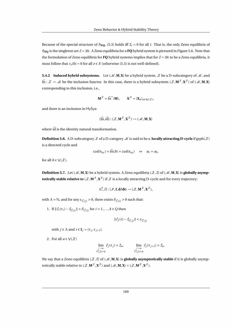
Zeno Behavior & Hybrid Stability Theory
Because of the special structure of HFQ, (5.3) holds iff ~zi = 0 for all i . That is, the only Zeno equilibria of
HFQ is the singleton set ~z = 0. A Zeno equilibria for a FQ hybrid system is pictured in Figure 5.6. Note that
the formulation of Zeno equilibria for FQ hybrid systems implies that for ~z = 0 to be a Zeno equilibria, it
must follow that re (0) = 0 for all e ∈ E (otherwise (5.3) is not well-defined).
5.4.2 Induced hybrid subsystems. Let (M ,M,X) be a hybrid system, Z be a D-subcategory of M , and
~In : Z → M be the inclusion functor. In this case, there is a hybrid subsystem (Z ,MZ ,XZ ) of (M ,M,X)
corresponding to this inclusion, i.e.,
MZ = ~In∗
(M), XZ = Xaa∈V(Z ),
and there is an inclusion in HySys:
(~In, ~id) : (Z ,MZ ,XZ ) ,→ (M ,M,X)
where ~id is the identity natural transformation.
Definition 5.6. A D-subcategory Z of a D-category M is said to be a locally attracting D-cycle if grph(Z )
is a directed cycle and
cod(sa1 ) = ~In(b) = cod(sa2 ) ⇒ a1 = a2,
for all b ∈V(Z ).
Definition 5.7. Let (M ,M,X) be a hybrid system. A Zeno equilibria (Z ,~z) of (M ,M,X) is globally asymp-
totically stable relative to (Z ,MZ ,XZ ) if Z is a locally attracting D-cycle and for every trajectory:
(~C ,~c) : (I ,I,d///dt) → (Z ,MZ ,XZ ),
with Λ=N, and for any ε~C ( j ) > 0, there exists δ~C (i ) > 0 such that:
1. If ‖~ci (τi )−~z~C (i )‖ < δ~C (i ) for i = 1, . . . , k ∈Q then
‖~c j (t )−~z~C ( j )‖ < ε~C ( j )
with j ∈Λ and t ∈ I j = [τ j ,τ j+1].
2. For all a ∈V(Z )
limj→∞
~C ( j )=a
~c j (τ j ) = ~za , limj→∞
~C ( j )=a
~c j (τ j+1) = ~za .
We say that a Zeno equilibria (Z ,~z) of (M ,M,X) is globally asymptotically stable if it is globally asymp-
totically stable relative to (Z ,MZ ,XZ ) and (M ,M,X) = (Z ,MZ ,XZ ).
169

Zeno Behavior & Hybrid Stability Theory
Region of Stability
,,,,
Figure 5.7: A graphical representation of the “local” nature of relatively globally asymptotically stable Zenoequilibria.
5.4.3 The global-local nature of Zeno equilibria. The definition of relative global asymptotic stability
implicitly makes some very subtle points. The first is that this type of stability is both local and global in
nature—hence the use of the words “global” and “relative” in the definition. While for traditional dynam-
ical systems this would seem contradictory, the complexity of hybrid systems requires us to view stability
in a much different light, i.e., we must expand the paradigm for stability.
To better explain the mixed global and local nature of relatively globally asymptotically stable
Zeno equilibria, we note that the term “global” is used because the hybrid subsystem (Z ,MZ ,XZ ) is glob-
ally stable to the Zeno equilibria; this also motivates the use of the word “relative” as (M ,M,X) is stable
relative to a hybrid subsystem. Finally, the local nature of this form of stability is in the discrete portion of
the hybrid system, rather than the continuous one. That is, the D-subcategory Z can be thought of as a
neighborhood inside the D-category M (see Figure 5.7, where the D-categories Z and M are represented
by graphs in order to make their orientations explicit). The condition on the inclusion functor given in the
definition is a condition that all edges (or morphisms) are pointing into the neighborhood.
5.4.4 Zeno equilibria and FQ hybrid systems. Zeno equilibria are intimately related to Zeno behavior
for first quadrant hybrid systems. While this relationship is established, it is useful to have a graphical
representation of the convergence to a Zeno equilibria in a FQ hybrid system; this can be found in Figure
5.8.
Proposition 5.2. If a first quadrant hybrid system HFQ is globally asymptotically stable at the Zeno equi-
libria ~z = 0, then every trajectory with Λ=N is Zeno.
Proof (sketch). For simplicity, we will assume that Γ consists of a single vertex and a single edge; consider-
ing larger cycles would amount to repeating the same argument on each vertex with subsequences of the
switching times. Because of asymptotic convergence of the sequence of initial conditions, ~ci (τi ), there
170
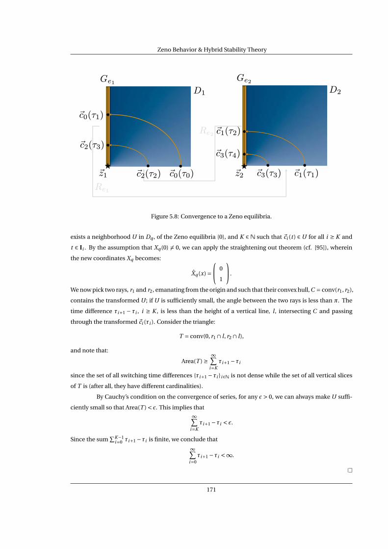
Zeno Behavior & Hybrid Stability Theory
D1Re1Re2Ge1 Ge2
Re2
Re1
D1 D2
Ge1 Ge2
~c0(τ1)
~c2(τ3)
~c2(τ2)~z1 ~c0(τ0)
~c1(τ2)
~c3(τ4)
~z2 ~c3(τ3) ~c1(τ1)
Figure 5.8: Convergence to a Zeno equilibria.
exists a neighborhood U in Dq , of the Zeno equilibria 0, and K ∈N such that ~ci (t ) ∈U for all i ≥ K and
t ∈ Ii . By the assumption that Xq (0) 6= 0, we can apply the straightening out theorem (cf. [95]), wherein
the new coordinates Xq becomes:
Xq (x) = 0
1
.
We now pick two rays, r1 and r2, emanating from the origin and such that their convex hull, C = conv(r1, r2),
contains the transformed U ; if U is sufficiently small, the angle between the two rays is less than π. The
time difference τi+1 − τi , i ≥ K , is less than the height of a vertical line, l , intersecting C and passing
through the transformed ~ci (τi ). Consider the triangle:
T = conv(0, r1 ∩ l , r2 ∩ l),
and note that:
Area(T ) ≥∞∑
i=Kτi+1 −τi
since the set of all switching time differences τi+1 −τi i∈N is not dense while the set of all vertical slices
of T is (after all, they have different cardinalities).
By Cauchy’s condition on the convergence of series, for any ε > 0, we can always make U suffi-
ciently small so that Area(T ) < ε. This implies that∞∑
i=Kτi+1 −τi < ε.
Since the sum∑K−1
i=0 τi+1 −τi is finite, we conclude that
∞∑i=0
τi+1 −τi <∞.
171

Zeno Behavior & Hybrid Stability Theory
5.4.c Conditions on Stability
We now give conditions on the stability of Zeno equilibria for first quadrant hybrid systems.
These will be instrumental in providing conditions on the stability of Zeno equilibria for general hybrid
systems.
5.4.5 Conditions for the stability of HFQ. In order to give conditions on the stability of Zeno equilib-
ria, it is necessary to give conditions on both the continuous and discrete portions of the hybrid system.
That is, the conditions on stability will relate to three aspects of the behavior of the hybrid system: the
continuous portion, the existence of events and the discrete portion.
Continuous conditions: For all i ∈Q,
(I) Xi (x) 6= 0 for all x ∈ (R+0 )2.
(II) There exists a function vi : (R+0 )2 → R+
0 of class K∞ along each ray emanating fromthe origin in Di and d(vi )x Xi (x) ≤ 0 for all x ∈ (R+
0 )2.
Event conditions: For all i ∈Q,
(III) (Xi (x1,0))2 ≥ 0.
Now consider the map ψi defined by requiring that:
ψi (x) = y if (0, y) = v−1i (vi (x,0))∩ x1 = 0 and x2 ≥ 0
which is well-defined by condition (II). Using ψi we introduce the function Pi :R+0 →R+
0 given by:
Pi (x) = rei−1 ψi−1 · · · re1 ψe1 rek ψek · · · re1 ψ1(x).
The map Pi can be thought of as both a Poincaré map or a discrete Lyapunov function depending on the
perspective taken. The final conditions are given by:
Discrete conditions: For all i ∈Q and e ∈ E ,
(IV) re is order preserving.
(V) There exists a class K∞ function α such that Pi (x)−x ≤−α(x).
Theorem 5.4. A first quadrant hybrid system HFQ is globally asymptotically stable at the Zeno equilibria
~z = 0 if conditions (I)− (V) hold.
Proof. Proving this result requires us to show three things: the existence of events, the boundedness of
trajectories and asymptotic convergence of the sequence of initial conditions.
We begin by demonstrating the existence of events; if c(0) is an initial condition of a solution
c(t ) of c = Xq (c) on Dq = (R+0 )2, then there exists an event if c(τ) ∈Geq for some finite τ, i.e., if (c(τ))1 = 0
and (c(t ))2 ≥ 0 for all t ∈ [0,τ]. To show that there exists an event, we must rule out two other possible
scenarios:
172

Zeno Behavior & Hybrid Stability Theory
1. The trajectory c(t ) exits Dq in finite time without intersecting the guard. In particular, since Dq =(R+
0 )2, this implies that there must exist a τ such that (c(τ))2 < 0 and (c(t ))1 > 0 for t ∈ [0,τ].
2. The trajectory never exits Dq , i.e., c(t ) ∈ Dq \Geq for all t .
We will show that conditions (I)− (III) exclude these scenarios.
Beginning with scenario 1, if (c(τ))2 < 0, since (c(0))2 ≥ 0, it follows by continuity that there exists
a t ∈ [0,τ] such that (c(t ))2 = 0 and (Xq (c(t )))2 < 0 for (c(t ))1 > 0. But these inequalities are ruled out by
condition (III).
For scenario 2, we first note that condition (II) implies that
|v−1q (vq (y))∩ x1 = 0 and x2 ≥ 0| = 1 (5.4)
|v−1q (vq (y))∩ x2 = 0 and x1 ≥ 0| = 1 (5.5)
for all y ∈ Di . Now define the set
Vq = x ∈ Dq : vq (x) ≤ vq (c(0)).
Note that the boundary of this set consists of three smooth components, i.e., a piece of the vertical axis
(the guard), a piece of the horizontal axis and a piece of the level set v−1q (vq (c(0))). We have already shown
that the solution cannot exit through the horizontal axis, and it cannot exit through the piece of the level
set (intersection Dq ) since we are supposing that d(vq )x Xq (x) ≤ 0 by condition (II). In view of this, if the
trajectory exits the set Vq , then it must exit through the guard, i.e., there must exist an event. Therefore,
we must show that the trajectory exits this set, i.e., that Vq is not an invariant set.
We are assuming that Vq is proper. Suppose, by way of contradiction, that Vq is an invari-
ant set. By the Poincaré-Bendixson theorem, because we are assuming that Vq contains no equilib-
rium points (condition (I)), it must contain a limit cycle: γ(t ) with γ(t ) = γ(t +T ). First suppose that
vq (γ(t )) ≡ c, then by condition (II) (and more specifically (5.4)), γ(t ) must intersect the vertical and hor-
izontal axis and because this is a one-dimensional limit cycle in two dimensional space it has an ori-
entation. Therefore, the assumption that γ(t ) is contained in Vq is violated. Alternatively, suppose that
vq (γ(t )) = c and vq (γ(t ′)) = c ′ for c > c ′ and some t < t ′ < T . By the periodicity of the γ(t ), this implies that
vq (γ(t ′)) < vq (γ(t +T )) = vq (γ(t )) = c, where t +T > t ′, which implies that d(vq )γ(t )Xq (γ(t )) ≥ 0 for some
t ∈ [t ′, t +T ], which violates condition (II).
We conclude that events must always exist.
Let us now address the issue of asymptotic convergence of the sequence of initial conditions.
Recalling the construction of (M FQ,MFQ,XFQ) from HFQ, for a trajectory
(I ,I,d///dt)(~C ,~c)- (M FQ,MFQ,XFQ),
we need to show that for all a ∈V(M FQ)
limj→∞
~C ( j )=a
~c j (τ j ) = 0. (5.6)
173

Zeno Behavior & Hybrid Stability Theory
Define Ψi (x,0) = (0,ψi (x))T . Starting from i > 1, ~ci (τi ) ∈ x1 ≥ 0 and x2 = 0 so
v~C (i )(~ci (τi+1)) ≤ v~C (i )(~ci (τi )) = v~C (i )(Ψ~C (i )(~ci (τi )))
from condition (II). Also by this condition, we can take the inverse of v~C (i ) because it is class K∞ along
every ray emanating from the origin (which intersects Dq ) and hence along the vertical axis, which implies
that
(~ci (τi+1))2 ≤ψ~C (i )((~ci (τi ))1).
Applying re to this inequality, which by condition (IV) is order preserving, yields
rei ((~ci (τi+1))2) ≤ rei (ψ~C (i )((~ci (τi ))1)).
By iterating this process k times, and noting that ~C (i +k) = ~C (i ), we have
(~ci+k (τi+k ))1 ≤ P~C (i )((~ci (τi ))1).
Therefore, the sequence (~ci+k (τi+k ))1 is bounded by the sequence P~C (i )((~ci (τi ))1) which converges to za in
view of (V). Convergence of ~ci (τi+1) now follows from convergence of ~ci (τi ) and the fact that ψi (~ci (τi )) =~ci (τi+1) is an order preserving function as vi is of class K∞ when restricted to the guard of domain Di .
Finally, boundedness of the continuous trajectories in each mode (and hence boundedness of
the sequence of initial conditions) follows from the existence of the Lyapunov function v~C (i ), i.e., by the
conditions given in (II), and by the fact that the map P~C (i ) satisfies condition (V).
Corollary 5.2. If HFQ is a first quadrant hybrid system satisfying conditions (I)−(V), then there exist trajec-
tories with Λ=N and every such trajectory is Zeno.
Note that the condition that Λ = N in Proposition 5.2 and Corollary 5.2 is due to the fact that
there always are trajectories with finite indexing setΛ, e.g., any trajectory withΛ=Nhas “sub-trajectories”
with finite indexing sets. These trajectories are trivially non-Zeno, so we necessarily rule them out.
Example 5.6. To verify that HballFQ is globally asymptotically stable at the Zeno point ~z = 0, and hence
Zeno by Proposition 5.2, we need only show that conditions (I)− (V) are satisfied. It is easy to see that
conditions (I) and (III) are satisfied (see Figure 5.9). Since re1 (x) = x and re2 (x) = ex, condition (IV) holds.
We use the original Hamiltonian
H(x1, x2) = 1
2x2
2 +mg x1,
suitably transformed, for the Lyapunov type functions given in (II), i.e., we pick:
v1(x1, x2) = 1
2x2
1 + g x2, v2(x1, x2) = 1
2x2
2 + g x1.
It is easy to see that these functions meet the specifications given in (II); some of the level sets of these
functions can be seen in Figure 5.9. Note that the level sets on one domain increase, but this is compen-
sated for by the decreasing level sets on the other domain. Finally, condition (V) is satisfied when e < 1
since
P1(x) = P2(x) = ex.
174

Zeno Behavior & Hybrid Stability Theory
Figure 5.9: Graphical verification of the properties (I)− (III) for the bouncing ball hybrid system for thefirst domain (left) and the second domain (right).
A graphical representation of the maps P1 and P2 can be seen in Figure 5.10.
5.4.d Hybrid Stability Theory
Building upon the results of the previous section, we are able to derive sufficient conditions for
the stability of general hybrid systems. Mirroring the continuous case, we simply find a morphism to the
“simplest stable object,” i.e., a first quadrant hybrid system. Formally:
Definition 5.8. Define GasZeno be the full subcategory of HySys consisting of first quadrant hybrid sys-
tems (M SFQ,MSFQ,XSFQ) that are globally asymptotically stable at the Zeno equilibria ~z = 0.
175

Zeno Behavior & Hybrid Stability Theory
Dball2Dball
1Gballe1 Gballe2
re2(x) = ex
ψ1(x)
ψ2(y)
re1(x) = x
xy
x
P1(x) = ex
x
P2(x) = ex
Figure 5.10: A graphical illustration of the construction of the functions P1 and P2 for the bouncing ball.
Theorem 5.5. A Zeno equilibria (Z ,~z) of (M ,M,X) is globally asymptotically stable relative to (Z ,MZ ,XZ )
if there exists a morphism of hybrid systems:
(Z ,MZ ,XZ )(~V ,~v)- (M SFQ,MSFQ,XSFQ) ∈GasZeno
in HySys satisfying, for all a ∈Ob(Z ),
1. ~va(x) = 0 implies x = ~za ,
2. ~va is a proper (radially unbounded) function.
An immediate, and very important, corollary of this theorem is that it yields sufficient conditions
for the existence of Zeno behavior.
Corollary 5.3. Under the assumptions of Theorem 5.5, there exist trajectories
(I ,I,d///dt)(~C ,~c)- (Z ,MZ ,XZ )
with Λ=V(I ) =N and every such trajectory is Zeno.
176

Zeno Behavior & Hybrid Stability Theory
Of course, a trajectory of (Z ,MZ ,XZ ) immediately yields a trajectory of (M ,M,X) through com-
position. That is,
(I ,I,d///dt)(~C ,~c)- (Z ,MZ ,XZ )
(~In,~id)- (M ,M,X)
is a trajectory of (M ,M,X). Therefore, we have given conditions for the existence of Zeno trajectories for
(M ,M,X).
Proof of Theorem 5.5. Let
(I ,I,d///dt)(~C ,~c)- (Z ,MZ ,XZ )
be a morphism where (I ,I,d///dt) ∈ Interval(HySys) and Λ=V(I ) =N. Assume that
‖~ci (τi )−~z~C (i )‖ ≤ δ~C (i )
for i = 1,2, . . . , k. This implies that ~ci (τi ) is contained in a compact set containing ~zC (i ). If we denote such
set by S ~C (i ), it follows by continuity of ~v~C (i ) that ~v~C (i )(S ~C (i )) is compact and that ~v~C (i )(~ci (τi )) ∈ ~v~C (i )(S ~C (i ))
and ~v~C (i )(~z~C (i )) ∈ ~v~C (i )(S ~C (i )). Taking into account that ~v~C (i )(~z~C (i )) = 0 we obtain:
‖~v~C (i ) ~ci (τi )−0‖ ≤ δ′~V~C (i ).
It now follows from global asymptotic stability of the Zeno equilibria (M SFQ,~z = 0) of (M SFQ,MSFQ,XSFQ)
that:
‖~v~C ( j ) ~c j (t )−0‖ ≤ ε′~V~C ( j ), t ∈ I j , j ∈Λ.
This inequality implies that ~v~C ( j ) ~c j (t ) belongs to a compact set for all t ∈ I j . Because ~v j is assumed to be
proper, there exists a ε~C ( j ) such that:
‖~c j (t )−~z~C ( j )‖ ≤ ε~C ( j ), t ∈ I j , j ∈Λ.
A similar argument yields, by the continuity of ~v~C ( j ), for all a ∈V(Z ) with ~C ( j ) = a,
limj→∞
~C ( j )=a
~c j (τ j ) = ~v −1~C ( j )
limj→∞
~V~C ( j )=~V (a)
~v~C ( j ) ~c j (τ j )
= ~v −1~C ( j )
(0) = ~za .
Theorem 5.5 is an important result in many respects.
¦ It would have been very difficult to obtain without our categorical framework for hybrid systems.
This indicates that categorical hybrid systems theory can yield results that are important, interesting
and novel.
¦ It yields a general method for studying the stability of hybrid systems. That is, any other type of
more “classical” stability that might be of interest—asymptotic stability, exponential stability, etc.—
can be studied using the same methodology. In fact, these types of stability are easier to study; this
is why we opted to study Zeno equilibria. For other types of stability, the “simplest” stable objects
will be one-dimensional hybrid systems with the desired stability property. These extensions follow
in a trivial manner from the framework established here.
177

Zeno Behavior & Hybrid Stability Theory
5.5 Going Beyond Zeno
Motivated by the fact that for a Zeno trajectory time never progresses past a certain time (the
Zeno time) and “point” (the Zeno point(s)), a natural—and intriguing—question to ask is:
What happens after a Zeno point?
Inspired by the construction of [50], we propose a method for extending Zeno executions past a Zeno
point for Lagrangian hybrid systems as were introduced in Chapter 3; for the sake of simplicity and con-
sistency, we revert to the notation utilized in that chapter.
Using the special structure of Lagrangian hybrid systems obtained from hybrid Lagrangians, we
are able to demonstrate that the Zeno point must satisfy constraints imposed by the unilateral constraint
function. These constraints are holonomic in nature, and this implies that after the Zeno point the hybrid
system should switch to a holonomically constrained dynamical system. The resulting system obtained
by “composing” the hybrid system with this dynamical system defines a completed hybrid system, which
inherently allows an execution to continue past the Zeno point. Although we do not prove that this is
the correct way to carry executions beyond Zeno points, we argue that our method correctly represents
the physical, post-Zeno, behavior of the system being modeled. In order to substantiate this argument,
we discuss how to practically implement a completed hybrid system and illustrate these concepts with a
series of examples.
5.5.1 Lagrangian hybrid systems and their executions. Here we quickly recall the notation from Chap-
ter 3, which will be in force throughout this section. First, recall from Definition 3.1 that a simple hybrid
Lagrangian is given by a tuple:
L = (Q,L, h).
Associated to a hybrid Lagrangian is a simple hybrid system,
HL = (DL,SL,RL,XL),
as constructed in Subsection 3.2.a; see Figure 5.11 for a graphical representation of a Lagrangian hybrid
system.
An execution of a Lagrangian hybrid system, which we referred to as a hybrid flow in order to
avoid confusion, is a tuple
εL = (Λ, I ,C )
as introduced in Paragraph 3.2.1. We will revert to the terminology “hybrid flow” to again differentiate
executions of this form from the ones considered in the rest of this chapter. In addition, we utilize the su-
perscript “L” to indicate that the hybrid flow is the hybrid flow of the Lagrangian hybrid system associated
to a hybrid Lagrangian.
We now introduce the notion of a Zeno point, which can be thought of as a form of Zeno equi-
libria for Lagrangian hybrid systems.
178

Zeno Behavior & Hybrid Stability Theory
RL(x)
DL
x = XL(x)
x ∈ SL
Figure 5.11: A Lagrangian hybrid system: HL.
Definition 5.9. The Zeno point of a Zeno hybrid flow εL is defined to be
x∞ = (q∞, q∞) = limi→∞
ci (τi ) = limi→∞
(qi (τi ), qi (τi )).
Here ci = (qi , qi ) ∈ C , and the Zeno point is necessarily a single point because of the specific problem
formulation considered in this section.
5.5.2 Zeno points. Lagrangian hybrid systems display both chattering and genuinely Zeno behavior;
roughly speaking, the coefficient of restitution can be used to differentiate between these systems. More-
over, Zeno points must satisfy certain constraints based on the unilateral constraint function. In order to
do so, let
A(q) =(
∂h∂q1
(q) · · · ∂h∂qn
(q))
.
Now, recalling the distinction between types of Zeno behavior made in Paragraph 5.1.3, we make the
following observations:
CZ: If HL has a chattering Zeno hybrid flow, εL, then τ∞ = τ1−τ0 and x∞ = (q1(τ1), q1(τ1)) withh(q1(τ1)) = 0 and A(q1(τ1))q1(τ1) = 0.
GZ: If HL has a genuinely Zeno hybrid flow, then 0 < e < 1. Moreover, if εL is a genuinely Zenohybrid flow, then x∞ = (q∞, q∞) is a point with h(q∞) = 0, and A(q∞)q∞ = 0.
Summarizing, our main observation is:
Main Observation. If εL is a Zeno hybrid flow of a Lagrangian hybrid system HL, then the Zenopoint x∞ = (q∞, q∞) is a point satisfying h(q∞) = 0 and A(q∞)q∞ = 0.
This observation indicates how the system should behave after the Zeno point, i.e., it should sat-
isfy a holonomic constraint. This holonomic constraint forces the system to slide along surface h−1(0) =q ∈ Q : h(q) = 0. From this we argue that after the Zeno point, the hybrid system should switch to a
holonomically constrained dynamical system.
179

Zeno Behavior & Hybrid Stability Theory
5.5.3 Holonomically constrained systems. Recall that for a holonomically constrained system described
by a Lagrangian, L, of the form given in (3.2), the equations of motion for the holonomically constrained
system are obtained from the equations of motion for the unconstrained system (3.3); they are given by
(cf. [93])
M(q)q +C (q, q)q +N(q)+ A(q)Tλ= 0,
where λ is the Lagrange multiplier, which in this case is given by
λ= (A(q)M(q)−1 A(q)T )−1 (˙A(q)q − A(q)M(q)−1(C (q, q)q +N(q))
).
From the constrained equations of motion, for x = (q, q), we get the vector field
x = X∞L (x)
= (q,M(q)−1(−C (q, q)q −N(q)− A(q)Tλ)
).
Note that the X∞L defines a vector field on the manifold TQ|h−1(0), from which we obtain the dynamical
system
D∞L = (TQ|h−1(0),X∞
L ).
This, when coupled with the Main Observation, will be essential to understanding how to carry hybrid
flows beyond Zeno points.
5.5.4 Completing hybrid systems. We begin by considering the case when HL is a chattering Zeno
hybrid system; in this case, the idea of carrying hybrid flows past the Zeno point has been well-studied. In
[50], it is argued that once the solution hits the “switching surface” (or in our case, the guard), the solution
should slide along the switching surface. In terms of Zeno points, this implies that before the Zeno point
the dynamics should be dictated by XL, while after the Zeno point the dynamics should be dictated by
X∞L . We can generalize this construction to include genuinely Zeno Lagrangian hybrid systems.
Definition 5.10. If HL is a Lagrangian hybrid system, we define the corresponding completed hybrid
system3 (or the completion of HL) as
HL := D∞
L if h(q) = 0 and A(q)q = 0
HL otherwise.
5.5.5 Completing trajectories. A completed hybrid system, as obtained from a Lagrangian hybrid sys-
tem HL, can be seen in Figure 5.12. To make the definition of the completed system somewhat more
transparent, some comments are in order. The Main Observation indicates that the only way for the tran-
sition to be made from the hybrid system HL to the dynamical system D∞L is if a specific Zeno hybrid
flow reaches its Zeno point. Therefore, before the Zeno point, the Zeno system simply will be the hybrid
3This terminology (and notation) is borrowed from topology, where a metric space can be completed to ensure that “limits exist.”
180

Zeno Behavior & Hybrid Stability Theory
RL(x)
DL
h(q) = 0
h(q) = 0 and A(q)q = 0
x = X∞L (x)x = XL(x)
x ∈ SL
Figure 5.12: A completed hybrid system: HL.
system HL, while after the Zeno point, the completed system will be the dynamical system D∞L . Since the
dynamical system forces the system dynamics to be constrained to the manifold defined by h−1(0), this
implies that the completed system will slide along the guard (switching surface) after the Zeno point.
This can be understood further on the level of hybrid flows. We can define a hybrid flow of the
completed hybrid system HL by concatenating a Zeno hybrid flow of HL with an integral curve of the
dynamical system D∞L .
Specifically, let εL = (N, I ,C ) be a Zeno hybrid flow of HL. We obtain a hybrid flow of the com-
pleted hybrid system HL by defining it to be
εHL = (N∪ ∞, I ,C ),
where
I = I ∪ I∞ = [τ∞,∞), C =C ∪ c∞,
with c∞(t ) an integral curve of X∞L with initial condition the Zeno point:
c∞(τ∞) = x∞ = (q∞, q∞).
We now discuss some practical issues related to simulating integral curves of completed systems.
5.5.6 Practical issues. We discuss two practical issues when modeling and simulating completed hy-
brid systems (see Figure 5.12). These issues are related to the transition from the left state HL to the right
state D∞L , and the corresponding initial conditions of D∞
L . The theoretical framework established in this
section allows us to justifiably surmount the practical problems introduced in simulation.
The first simulation issue is derived from the unavoidable numerical errors that result from the
finite representation of values in a computer and truncation errors introduced by practical ODE solvers,
i.e., a simulator produces an approximate hybrid flow εL to the hybrid flow εL. Therefore, we cannot guar-
antee or expect an integral curve of reach the exact Zeno point x∞ = (q∞, q∞). Moreover, in order to reach
181

Zeno Behavior & Hybrid Stability Theory
the Zeno point, an infinite number of computation steps have to be performed (in a finite amount of
time). Therefore, instead of resolving a solution that passes through the Zeno point exactly, we will com-
pute an approximation of the Zeno solution; the approximated solution will pass through a neighborhood
of the Zeno point, so we must modify the transition to the system D∞L accordingly. Before discussing the
details of the construction of the approximate solution, we first address the second modeling issue.
The other concern is the reinitialization of the new constrained system D∞L . In other words, after
the transition to this system, we must give initial conditions for the constrained system. Theoretically, the
initial condition is the Zeno point, but because in simulation we do not actually reach the Zeno point, an
initial condition must be estimated—one that satisfies the same conditions as a Zeno point: h(q∞) = 0
and A(q∞)q∞ = 0.
5.5.7 Approximating completed systems. The approximation to the completed hybrid system HL, de-
noted by Hδ
L , is given by
Hδ
L := D∞
L if abs(h(q)) ≤ δ and abs(A(q)q) ≤ δ
HL otherwise
for some δ > 0. When switching from HL to D∞L via the approximated guard condition, we use a map
which resets the variables so that they satisfy the conditions of a Zeno point: h(q∞) = 0 and A(q∞)q∞ = 0.
Specifically, for a point (q, q) satisfying the approximate guard condition
abs(h(q)) ≤ δ and abs(A(q)q) ≤ δ,
we define a reset map R∞ which sends (q, q) to an approximate Zeno point, (q∞, q∞) = R∞(q, q), satisfying
h(q∞) = 0 and A(q∞) q∞ = 0.
We now briefly discuss how to construct the map R∞ for the running examples in this section. In all of
these examples, the vector fields for the constrained dynamical systems are easy to calculate.
Example 5.7. Again consider the hybrid system modeling a bouncing ball on a sinusoidal surface, HB, as
first introduced in Example 3.5. In this example, the vector field for the holonomically constrained system
D∞B is given by
X∞B (q, q) =
q,
0
2cos(x2)(−g+sin(x2)x22)
3+cos(2x2)
− 2(g cos(x2)2+sin(x2)x22)
3+cos(2x2)
.
Note that
hB(x) = 0 ⇒ x3 = sin(x2),
AB(x)x = 0 ⇒ x3 −cos(x2)x2 = 0.
182

Zeno Behavior & Hybrid Stability Theory
x1_dotx2_dotx3_dot
-6
-4
-2
0
2
4
0.0 0.2 0.4 0.6 0.8 1.0 1.2 1.4 1.6 1.8 2.0
Velocities
time
velo
citie
s
x1x2x3
-3
-2
-1
0
1
2
0.0 0.2 0.4 0.6 0.8 1.0 1.2 1.4 1.6 1.8 2.0
Displacements
time
disp
lace
men
ts
-1.0
-0.5
0.0
0.5
1.0
1.5
2.0
-3.5 -3.0 -2.5 -2.0 -1.5 -1.0 -0.5 0.0 0.5 1.0
Displacement: x3 vs. x2
displacement x2
disp
lace
men
t x3
Figure 5.13: Simulation gets stuck at the Zeno point. Velocities over the time (top), displacements over thetime (middle) and displacement on the x3 direction vs. the displacement on the x2 direction (bottom).
183

Zeno Behavior & Hybrid Stability Theory
x1_dotx2_dotx3_dot
-6
-4
-2
0
2
4
0.0 0.5 1.0 1.5 2.0 2.5 3.0 3.5 4.0 4.5 5.0 5.5 6.0
Velocities
time
velo
citie
s
x1x2x3
-3
-2
-1
0
1
2
3
0.0 0.5 1.0 1.5 2.0 2.5 3.0 3.5 4.0 4.5 5.0 5.5 6.0
Displacements
time
disp
lace
men
ts
-1.0
-0.5
0.0
0.5
1.0
1.5
2.0
-3.5 -3.0 -2.5 -2.0 -1.5 -1.0 -0.5 0.0 0.5 1.0
Displacement: x3 vs. x2
displacement x2
disp
lace
men
t x3
Figure 5.14: Simulation goes beyond the Zeno point. Velocities over the time (top), displacements overthe time (middle) and displacement on the x3 direction vs. the displacement on the x2 direction (bottom).
184

Zeno Behavior & Hybrid Stability Theory
And so we define the approximate reset map as:
R∞B (x1, x2, x3, x1, x2, x3) =
x1
x2
sin(x2)
,
x1
x2
cos(x2)x2
.
We begin by simulating the "non-completed" hybrid system HB, the results of which are shown
in Figure 5.13 (to which the rest of the paragraph refers). The simulation time is set to 6.0, but the sim-
ulation gets stuck at around 2.04; the bottom figure indicates that the ball tries, but is unable, to climb
upwards along the surface (a sinusoidal waveform). Its velocities decrease during this process due to the
energy loss through impact as can be seen in the top figure. As a consequence, more and more collisions
are triggered and the time interval between two consecutive collisions keeps shrinking. The dense points
near time 2.04 in the middle figure indicate that more and more computation steps are taken, which
makes the simulation halt. This behavior is indicative of genuinely Zeno behavior.
Figure 5.14 shows a simulation of the completed hybrid system Hδ
B with the same initial condi-
tions. Note that the simulation closely approaches the Zeno point before the behavior of the ball auto-
matically switches to what X∞B specifies, i.e., the ball oscillates along the surface (a sinusoidal waveform).
Therefore, the simulation does not halt, freely moving beyond the Zeno point in a manner consistent with
physical reality.
Example 5.8. Now consider the hybrid system modeling a pendulum on a cart, HC, as introduced in
Example 3.6. The vector field for the holonomically constrained system D∞C is given by
X∞C (q, q) =
q,
−cot(θ)θ2
mR csc(θ)θ2
M+m
.
Note that
hC(q) = 0 ⇒ cos(θ) = 0
AC(q)q = 0 ⇒ sin(θ)θ= 0.
From the above two equations, we can compute precisely that θ = sign(θ)π/2 and θ = 0. The rest of the
variables x and x have no extra constraints. Therefore, the complete reset map is:
R∞C (θ, x, θ, x) =
sign(θ)π/2
x
,
0
x
.
Simulation verifies that the completed version of this hybrid system has the correct post-Zeno behavior;
see Figure 5.15.
Example 5.9. As a final example, consider the hybrid system modeling a pendulum mounted on the floor,
HP, as introduced in Example 3.7. Although this system was introduced as a Hamiltonian hybrid system, it
can be converted without difficulty to a Lagrangian hybrid system through the Legendre transformation.
185

Zeno Behavior & Hybrid Stability Theory
theta_dotx_dot
-1.5
-1.0
-0.5
0.0
0.5
1.0
0 5 10 15 20 25 30 35 40
Velocities
xtheta
-8-7
-6
-5
-4
-3
-2
-1
0
0 5 10 15 20 25 30 35 40
Positions
Figure 5.15: Simulation of the Cart that goes beyond the Zeno point. Velocities over the time (top) anddisplacements over the time (bottom).
In this example, the vector field for the holonomically constrained system D∞P is given by
X∞P (q, q) =
q,
−cot(θ)θ2
−2cot(θ)θϕ
.
Note that
hP(q∞) = 0 ⇒ cos(θ) = 0
AP(q∞)q∞ = 0 ⇒ sin(θ)θ= 0.
From the above two equations, we can calculate precisely that θ=π/2 and θ= 0. Therefore, the complete
reset map is:
R∞P (θ,ϕ, θ,ϕ) =
π/2
ϕ
,
0
ϕ
.
Simulation verifies that the completed version of this hybrid system has the correct post-Zeno behavior;
See Figure 5.16.
186

Zeno Behavior & Hybrid Stability Theory
theta_dotphi_dot
-1.0
-0.5
0.0
0.5
1.0
1.5
0 5 10 15 20 25 30 35
Angular Velocities
thetaphi
0.51.0
1.5
2.0
2.5
3.0
3.5
4.0
4.5
5.0
0 5 10 15 20 25 30 35
Angles
Figure 5.16: Simulation of the Pendulum goes beyond the Zeno point. Angular velocities over the time(top) and angles over the time (bottom).
187

Part III
Networked Systems
188

Chapter 6
Universally Composing Embedded
Systems
In an embedded system, different components of the system evolve according to processes lo-
cal to the specific components. Across the entire system, these typically heterogeneous processes may
not be compatible, i.e., answering questions regarding the concurrency, timing and causality of the en-
tire system—all of which are vital in the actual physical implementation of the system—can be challeng-
ing even if these questions can be answered for specific components. Denotational semantics provide
a mathematical framework in which to study the behavior (signals, flows, executions, traces) of embed-
ded systems or networks thereof. This framework is naturally applicable to the study of heterogeneous
networks of embedded systems since signals always can be compared, regardless of the specific model of
computation from which they were produced.
Tagged systems provide a denotational semantics for heterogeneous models of computation;
they consist of a set of tags (a tag structure), variables and maps (behaviors) from the set of variables to
the set of tags—hence, tagged systems are a specific case of the tagged signal model (cf. [76]). A heteroge-
neous network of embedded systems, e.g., a network consisting of both synchronous and asynchronous
systems, can be modeled by a network of tagged systems with heterogeneous tag structures communi-
cating through mediator tagged systems. Benveniste et al. [22], [23] and [24], introduced the notion of
tagged systems and dealt with the issues we set forth in this chapter; this work extends and generalizes
the ideas introduced in these papers. Of course, there is a wealth of literature on semantics preservation
in heterogeneous networks, cf. [25], [40], [77], [97], and [117], the last of which approaches the problem
from a categorical prospective.
A network of tagged systems can be implemented, or deployed, through heterogeneous par-
allel composition—obtained by taking the conjunction (intersection) of the behaviors that agree on the
mediator tagged systems—which results in a single, homogeneous, tagged system. Thus, heterogeneous
networks of tagged systems can be homogenized through the operation of composition. This chapter
189
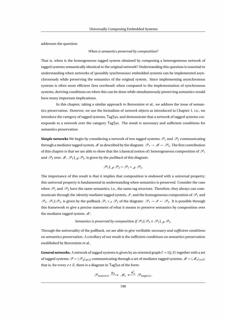
Universally Composing Embedded Systems
addresses the question:
When is semantics preserved by composition?
That is, when is the homogeneous tagged system obtained by composing a heterogeneous network of
tagged systems semantically identical to the original network? Understanding this question is essential to
understanding when networks of (possibly synchronous) embedded systems can be implemented asyn-
chronously while preserving the semantics of the original system. Since implementing asynchronous
systems is often more efficient (less overhead) when compared to the implementation of synchronous
systems, deriving conditions on when this can be done while simultaneously preserving semantics would
have many important implications.
In this chapter, taking a similar approach to Benveniste et al., we address the issue of seman-
tics preservation. However, we use the formalism of network objects as introduced in Chapter 1, i.e., we
introduce the category of tagged systems, TagSys, and demonstrate that a network of tagged systems cor-
responds to a network over the category TagSys. The result is necessary and sufficient conditions for
semantics preservation.
Simple networks We begin by considering a network of two tagged systems P1 and P2 communicating
through a mediator tagged system M as described by the diagram: P1 →M ←P2. The first contribution
of this chapter is that we are able to show that the (classical notion of) heterogeneous composition of P1
and P2 over M , P1‖M P2, is given by the pullback of this diagram:
P1‖M P2 =P1 ×M P2.
The importance of this result is that it implies that composition is endowed with a universal property;
this universal property is fundamental in understanding when semantics is preserved. Consider the case
when P1 and P2 have the same semantics, i.e., the same tag structure. Therefore, they always can com-
municate through the identity mediator tagged system, I , and the homogeneous composition of P1 and
P2, P1‖P2, is given by the pullback P1 ×I P2 of the diagram: P1 → I ← P2. It is possible through
this framework to give a precise statement of what it means to preserve semantics by composition over
the mediator tagged system M :
Semantics is preserved by composition if P1‖P2 ≡P1‖M P2.
Through the universality of the pullback, we are able to give verifiable necessary and sufficient conditions
on semantics preservation. A corollary of our result is the sufficient conditions on semantics preservation
established by Benveniste et al..
General networks. A network of tagged systems is given by an oriented graph Γ= (Q,E) together with a set
of tagged systems P = Pq q∈Q communicating through a set of mediator tagged systems M = Me e∈E ;
that is, for every e ∈ E , there is a diagram in TagSys of the form:
Psource(e)αe- Me
α′e Ptarget(e).
190

Universally Composing Embedded Systems
Equivalently, a network of tagged systems is given by a network over the category TagSys,
N(P ,M ,α) : NΓ →TagSys,
where NΓ is a Dop-category obtained from Γ (see Section 1.5). As in the case of a network of two tagged
systems, the heterogeneous composition of a network of tagged systems is given by the limit of this dia-
gram,
‖M P = LimNΓ(N(P ,M ,α)),
and so composition again is defined by a universal property.
If all of the P ′i s have the same semantics, then we can again consider the identity mediator I
(which in this case is a set) for which there are associated diagrams in TagSys of the form:
Psource(e)Rese- Me
Res′e Ptarget(e)
with Rese and Res′e restriction maps. To this network of tagged systems there is a corresponding network
object, N(P ,I ,Res) : NΓ →TagSys, and the homogeneous composition of this network is given by
‖P = LimNΓ(N(P ,I ,Res)).
The categorical formulation of networks of tagged systems allows us to give a precise statement
of when semantics is preserved:
Semantics is preserved by composition if ‖M P ≡ ‖P .
The universality of composition allows us to derive concrete necessary and sufficient conditions on when
semantics is preserved, indicating that this framework can produce results on semantics preservation that
are both practical and verifiable.
Extensions. Although this work is centered around the formalism of tagged system, the results are easily
extendable to arbitrary networks over categories and the composition thereof. That is, this work is the
first step toward addressing the general question of how to compose systems in a general and systematic
fashion in order to ensure that the composite system has the proper behavior.
Notation 6.1. In this section, we use calligraphic symbols to denote tag structures and tag systems; do not
confuse these with D-categories (which will not be utilized in this section, although Dop-categories will
be). The reason for this notation is historical precedence. Note that this is why we denote a Dop-category
by the symbol N (not to be confused with a hybrid system).
6.1 Universal Heterogeneous Composition
In this section, we begin by defining the category of tag structures. This definition is used to
understand how to associate a common tag structure to a pair of tag structures which can communicate
191

Universally Composing Embedded Systems
through a mediator tag structure. We then introduce the category of tagged systems, which will be instru-
mental in understanding how to form the heterogeneous composition of a network of tagged systems.
Finally, we discuss how to take the composition of a “simple” network of embedded systems.
Given two tagged systems, P1 and P2, we would like to form their composition, i.e., a single
tagged system obtainable from these two tagged systems. We begin by reviewing the “standard” definition
of composition, followed by a categorical reformulation of composition. We demonstrate that the com-
position of two tagged systems corresponds to the pullback of a specific diagram in the category of tagged
systems. This will allow us later to generalize the notion of composition.
6.1.1 Tag structures and the corresponding category. Fundamental to the notion of tagged systems is
the notion of timing. This timing is encoded in a set of tags; these “tag" the occurrences of events, i.e., they
index the events such that they are (partially) ordered. Hence, a set of tags or a tag structure is a partially
ordered set T , with the partial order denoted by ≤. The category of tags, Tag, can be defined as follows:
Objects: Partially ordered sets, i.e., tag structures.Morphisms: Nondecreasing maps between sets ρ : T → T ′, i.e., if t ≤ t ′ ∈ T then ρ(t ) ≤
ρ(t ′) ∈T ′.Composition: The standard composition of maps between sets.
Clearly, two objects in the category Tag are isomorphic if ρ : T → T ′ is a bijection: there exists a ρ′ :
T ′ → T such that ρ ρ′ = idT ′ and ρ′ ρ = idT . Note also that the terminal objects in the category Tag
are just one point sets Ttriv := ∗ (called asynchronous tag structures), i.e., for all tag structures T there
exists a unique morphism ρ : T → Ttriv defined by ρ(t ) ≡ ∗ which desynchronizes the tag structure. The
synchronous tag structure is given by Tsync =N.
6.1.2 Common tag structures. Tags are fundamental in understanding tagged systems in that mor-
phisms of tag structures will induce morphisms of tagged systems. To better understand this, we will dis-
cuss an important operation on tag structures: the pullback (the pullback of elements in a category will be
used extensively in the chapter—see Appendix A for a formal definition). Consider two tag structures T1
and T2. We would like to find a tag structure that is more general than T1 and T2 and has morphisms to
both of these tag structures, i.e., we would like to find a common tag structure for these two tag structures.
To do this, first consider the diagram in Tag:
T1ρ1 - T ρ2
T2, (6.1)
where T is the mediator tag structure. We know that such a tag structure always exists since it always can
be taken to be Ttriv (although this rarely is the wisest choice). We define the common tag structure to be
the pullback (see Paragraph A.2.3) of this diagram:
T1 ×T T2 = (t1, t2) ∈T1 ×T2 : ρ1(t1) = ρ(t2). (6.2)
192

Universally Composing Embedded Systems
Events
t1t2 t4t3 t5 t8t7
σ(1, x)
σ(2, x)
σ(6, x)
Tags (timing)
t6
Figure 6.1: A graphical representation of a behavior of a tagged system.
The pullback is the desired common tag structure since it sits in a commutative diagram of the form:
T1 ×T T2π2 - T2
T1
π1
? ρ1 - T
ρ2
?
(6.3)
Moreover, that fact that the common tag structure is the pullback implies that for any other tag structure
that displays the properties of a common tag structure, there exists a unique morphism from this tag
structure to the common tag structure. More precisely, for any tag structure T such that the following
diagram commutes:
T
T1 ×T T2 π2
-
∃!-
T2
q2
-
T1
π1
? ρ1 -
q1
-
T
ρ2
?
(6.4)
there exists a unique morphism from T to T1 ×T T2 also making the diagram commute. This construc-
tion on tag structures both motivates and mirrors constructions that will be performed throughout this
chapter on tagged systems. To demonstrate this we must, as with tag structures, define tagged systems
and the associated category.
6.1.3 Tagged systems. Following from [22], [23] and [24] (although our notation slightly deviates from
theirs), we define a tagged system. We then proceed to introduce the category of tagged systems.
193

Universally Composing Embedded Systems
Let V be an underlying set of variables and D be the set of values that these variables can take,
i.e., the domain of the variables. A tagged system is a tuple
P = (V,T ,Σ),
where V is a finite subset of the underlying set of variables V , T is a tag structure, i.e., an object of Tag,
and Σ is a set of maps:
σ :N×V →T ×D.
Each of the elements of Σ, i.e., each of the maps σ, are referred to as V -behaviors (or just behaviors when
the variable set is understood). It is required that for each v ∈ V , the map δv (n) :=π1(σ(n, v)) :N→T is a
morphism in Tag, that is, nondecreasing (and called a clock in [24]).
Remark 6.1. In defining the set of behaviors of a tagged system, we made an explicit choice for the domain
of the behaviors: N×V . This choice is motivated by the fact that the behaviors of a tagged system are
signals generated by a computer, and hence discrete in nature. It is possible to consider other domains
for the behaviors, e.g., R×V , without any significant change to the theory introduced here. This indicates
an interesting extension of this work to behavioral dynamical system theory (cf. [98, 111, 112]).
6.1.4 The category of tagged systems. We can use the formulation of tagged systems above in order to
define the category of tagged systems, TagSys, as follows:
Objects: Tagged systems P = (V,T ,Σ).Morphisms: A morphism of tagged systems α : P = (V,T ,Σ) → P ′ = (V ′,T ′,Σ′) is a mor-
phism (in the category of sets) of behaviors α : Σ→Σ′.Composition: The standard composition of maps between sets. In other words, for α : P →
P ′ and α′ : P ′ →P ′′ the composition of α : Σ→Σ′ and α′ : Σ′ →Σ′′ is given by α′ α : Σ→Σ′′.
From the definition of morphisms in the category TagSys, it follows that two tagged systems, P and P ′,
are isomorphic, P ∼=P ′, if and only if, to use the terminology from the literature, the two tagged systems
are in bijective correspondence.
6.1.5 A “forgetful” functor. By the definition of the category TagSys, there is a fully faithful functor:
B : TagSys→ Set,
where Set is the category of sets. This functor is defined on objects and morphisms in TagSys as follows:
for every diagram in TagSys of the form:
P = (V,T ,Σ)α→P ′ = (V ′,T ′,Σ′),
the functor B is given by:
B(P = (V,T ,Σ)
α→P ′ = (V ′,T ′,Σ′))=Σ
α→Σ′.
194

Universally Composing Embedded Systems
When discussing composition, we often will blur the distinction between the categories TagSys and Set,
i.e., we often will define the composition of a diagram of tagged systems by the behaviors of the composite
system, and hence implicitly view it as an object of Set. In this case, we always will construct an object in
TagSys with behaviors isomorphic to the corresponding object in Set.
6.1.6 Induced morphisms of tagged systems. Suppose that there is a morphism of tag structures ρ :
T → T ′. Then there exists a tagged system Pρ together with an induced morphism of tagged systems
( · )ρ : P →Pρ. First, if P = (V,T ,Σ) we define Pρ = (V,T ′,Σρ) where
Σρ := σρ :N×V →T ′×D :σρ(n, v) = (ρ(t ), d) iff (t , d) =σ(n, v)
for some σ ∈Σ.
That is, Σρ is defined by replacing t with ρ(t ) in the codomain of σ. With this definition of Pρ, we obtain
a morphism ( · )ρ : P →Pρ, called the desynchronization morphism and defined by, for each σ ∈Σ,
σρ(n, v) = (ρ(t ), d)def⇔ σ(n, v) = (t , d).
Note that ( · )ρ is always surjective.
Example 6.1. Consider the following synchronous tagged systems, P1 and P2, defined as follows:
P1 := (V1 = x,Tsync =N,Σ1 = σ1),
P2 := (V2 = x, y,Tsync =N,Σ2 = σ2, σ2),
where
σ1(n, x) := (m(n),?),
σ2(n, v) := (m(n),?) if v = x ∈ V2
(k(n),?) if v = y ∈ V2
,
σ2(n, v) := (m(n),?) if v = x ∈ V2
(l(n),?) if v = y ∈ V2
.
Here m(n), k(n) and l(n) are any strictly increasing functions with k(n) 6= l(n), and ? is a (single) arbitrary
value in D.
For ρ : Tsync →Ttriv the desyncronization morphism, P1∼=P
ρ1 because P1 consists of a single
behavior. Since Σ2 = σ2, σ2, Σρ2 = σρ2 = σρ2 , i.e., Σρ2 consists of a single behavior. Therefore, P2 is not in
bijective correspondence with Pρ2
6.1.7 Heterogeneous composition. Let P1 = (V1,T1,Σ1) and P2 = (V2,T2,Σ2) be two tagged systems.
Consider a mediator tag structure T between the tag structures T1 and T2, i.e., there exists a diagram in
Tag:
T1ρ1 - T ρ2
T2.
195
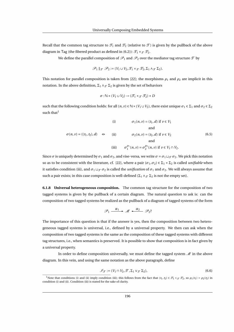
Universally Composing Embedded Systems
Recall that the common tag structure to T1 and T2 (relative to T ) is given by the pullback of the above
diagram in Tag (the fibered product as defined in (6.2)): T1 ×T T2.
We define the parallel composition of P1 and P2 over the mediator tag structure T by
P1 ∥T P2 := (V1 ∪V2,T1 ×T T2,Σ1 ∧T Σ2).
This notation for parallel composition is taken from [22]; the morphisms ρ1 and ρ2 are implicit in this
notation. In the above definition, Σ1 ∧T Σ2 is given by the set of behaviors
σ :N× (V1 ∪V2) → (T1 ×T T2)×D
such that the following condition holds: for all (n, v) ∈N×(V1∪V2), there exist unique σ1 ∈Σ1 and σ2 ∈Σ2
such that1
σ(n, v) = ((t1, t2), d) ⇔
(i) σ1(n, v) = (t1, d) if v ∈ V1
and
(ii) σ2(n, v) = (t2, d) if v ∈ V2
and
(iii) σρ11 (n, v) =σ
ρ22 (n, v) if v ∈ V1 ∩V2.
(6.5)
Sinceσ is uniquely determined byσ1 andσ2, and vise-versa, we writeσ=σ1tT σ2. We pick this notation
so as to be consistent with the literature, cf. [22], where a pair (σ1,σ2) ∈ Σ1 ×Σ2 is called unifiable when
it satisfies condition (iii), and σ1 tT σ2 is called the unification of σ1 and σ2. We will always assume that
such a pair exists; in this case composition is well-defined (Σ1 ∧T Σ2 is not the empty set).
6.1.8 Universal heterogeneous composition. The common tag structure for the composition of two
tagged systems is given by the pullback of a certain diagram. The natural question to ask is: can the
composition of two tagged systems be realized as the pullback of a diagram of tagged systems of the form
P1α1- M α2 P2?
The importance of this question is that if the answer is yes, then the composition between two hetero-
geneous tagged systems is universal, i.e., defined by a universal property. We then can ask when the
composition of two tagged systems is the same as the composition of these tagged systems with different
tag structures, i.e., when semantics is preserved. It is possible to show that composition is in fact given by
a universal property.
In order to define composition universally, we must define the tagged system M in the above
diagram. In this vein, and using the same notation as the above paragraph, define
IT := (V1 ∩V2,T ,Σ1 ∨T Σ2), (6.6)
1Note that conditions (i) and (ii) imply condition (iii); this follows from the fact that (t1, t2) ∈ T1 ×T T2, so ρ1(t1) = ρ2(t2) incondition (i) and (ii). Condition (iii) is stated for the sake of clarity.
196

Universally Composing Embedded Systems
where T is a mediator tag structure (between T1 and T2) and
Σ1 ∨T Σ2 := σ :N× (V1 ∩V2) →T ×D :
σ=σρii |V1∩V2 , for σi ∈Σi , i = 1 or 2. (6.7)
Now for the tagged systems P1 and P2 there exist morphisms
P1Resρ1
1- ITResρ2
2 P2 (6.8)
defined as follows:
Resρii (σi ) =σ
ρii |V1∩V2 :N× (V1 ∩V2) →T ×D
for σi ∈Σi , i = 1,2. Clearly, such a morphism always exists.
Note that IT is a mediator tagged system or channel between the tagged systems P1 and P2;
IT “communicates" between P1 and P2. In the case when T =T1 =T2, I :=IT is exactly the identity
mediator tagged system or identity channel introduced in [22].
Theorem 6.1. Consider two tagged systems P1 = (V1,T1,Σ1) and P2 = (V2,T2,Σ2) with mediator tag
structure T , i.e., suppose that there is a diagram in Tag:
T1ρ1 - T ρ2
T2.
The parallel composition of P1 and P2 over this tag structure, P1 ∥T P2, is the pullback of the diagram:
P1Resρ1
1- ITResρ2
2 P2
in the category of tagged systems, TagSys.
6.1.9 Implications of Theorem 6.1. Before proving Theorem 6.1, we discuss some of the implications
of this theorem.
If we consider the following diagram in the category of sets, Set:
Σ1Resρ1
1- Σ1 ∨T Σ2Resρ2
2Σ2 = B
(P1
Resρ11- IT
Resρ2
2 P2
),
the pullback of this diagram is given by:
Σ1 ×Σ1∨T Σ2 Σ2 = (σ1,σ2) ∈Σ1 ×Σ2 : Resρ11 (σ1) = Resρ2
2 (σ2).
It is important to note that the pullback of the above diagram (which is an object in Set) is related to—
in fact, isomorphic to—the behavior of the tagged system P1 ∥T P2. More precisely, for the functor
B : TagSys→ Set, we have:
Σ1 ×Σ1∨T Σ2 Σ2∼= B(P1 ∥T P2) =Σ1 ∨T Σ2. (6.9)
197

Universally Composing Embedded Systems
This observation will allow us later to, justifiably, blur the distinction between pullbacks (and limits) in
the categories TagSys and Set.
In order to produce the bijection given in (6.9), first note that there are projections defined by:
πi : Σ1 ∧T Σ2 →Σi (6.10)
where for each σ1 tT σ2 ∈ Σ1 ∧T Σ2, πi (σ1 tT σ2) := σi for i = 1,2. Because of (6.5), it follows that any
element σ ∈Σ1 ∧T Σ2 can be written as σ=π1(σ)tT π2(σ).
Theorem 6.1 implies—by the universality of the pullback—that there is a bijection:
(π1,π2) : Σ1 ∧T Σ2∼−→ Σ1 ×Σ1∨T Σ2 Σ2 (6.11)
σ=σ1 tT σ2 7→ (σ1 =π1(σ),σ2 =π2(σ))
where the inverse of this map is the unification operator:
( · )tT ( · ) : Σ1 ×Σ1∨T Σ2 Σ2∼−→ Σ1 ∧T Σ2 (6.12)
(σ1,σ2) 7→ σ1 tT σ2.
This completes the description of the bijection given in (6.9).
Proof. (of Theorem 6.1) From the definition of Σ1∧T Σ2 and Σ1∨T Σ2, it follows that the following diagram
in Set:
Σ1 ∧T Σ2π1 - Σ1
Σ2
π2
? Resρ22- Σ1 ∨T Σ2
Resρ11
?
commutes, which implies, by the definition of morphisms of tagged systems, that the following diagram
in TagSys:
P1 ∥T P2π1 - P1
P2
π2
? Resρ22- IT
Resρ11
?
commutes. Consider a tagged system Q such that the following diagram commutes:
Qq1 - P1
P2
q2
? Resρ22- IT
Resρ11
?
We can define a morphism γ : Q →P1 ∥T P2 by, for σ ∈ΣQ ,
γ(σ) = q1(σ)tT q1(σ).
198

Universally Composing Embedded Systems
It follows that there is a commuting diagram:
Q
P1 ∥T P2 π1
-
γ-
P1
q1
-
P2
π2? Resρ2
2 -
q2
-
IT
Resρ11
?
Moreover, by replacing γ with any other morphism making the diagram commute, say γ, it follows that
for σ ∈ΣQ
γ(σ) =π1(γ(σ))tT π2(γ(σ)) = q1(σ)tT q2(σ) = γ(σ).
So γ= γ, i.e., γ is unique.
6.2 Equivalent Deployments of Tagged Systems
Standard composition is just the pullback of a specific diagram in TagSys; this observation nat-
urally allows us to generalize composition. To perform this generalization, we introduce the notion of a
general mediator tagged system, M , and define composition to be the pullback of a diagram of the form:
P1α1- M α2 P2 (6.13)
in TagSys. This process will be instrumental later in understanding how to take the composition of more
general networks of embedded systems.
We conclude this section by reviewing the definition of semantics preservation and giving nec-
essary and sufficient conditions on when semantics is preserved. We apply these results to the special
case of semantics preservation through desyncronization.
6.2.1 Composition through mediation. Given the results of Theorem 6.1, we can develop a more intu-
itive notation for composition. Specifically, if T is the mediator tag structure, then we write P1 ∥T P2 =P1‖IT
P2 (in the case when T1 = T2 = T and ρ1 = ρ2 = id in (6.1), we just write P1‖P2 := P1‖I P2).
The mathematical reason for this is that P1‖ITP2 is (isomorphic to) P1 ×IT
P2, i.e., the pullback of
the diagram given in (6.8). The philosophical motivation for this notation is that the composition of P1
and P2 can be taken over general mediator tagged systems. In other words, the parallel composition of
P1 and P2 over a general mediator tagged system M , denoted by P1‖M P2, is defined to be the pullback
of the diagram given in (6.13):
P1‖M P2 :=P1 ×M P2.
This implies that if ΣM is the set of behaviors of M , then the set of behaviors for P1‖M P2 is isomorphic
to:
Σ1 ×ΣM Σ2 = (σ1,σ2) ∈Σ1 ×Σ2 :α1(σ1) =α2(σ2). (6.14)
199

Universally Composing Embedded Systems
The explicit construction of P1‖M P2 as a tagged system is not especially relevant, as we are interested
only in its set of behaviors which must be isomorphic to the set of behaviors given in (6.14). That being
said, this construction is a special case of a more general construction (given in Section 6.4) for which the
construction of the tagged system is carried out. We only note that there are bijections
( · )tM ( · ) : Σ1 ×ΣM Σ2∼−→ ΣP1‖MP2
(6.15)
(π1,π2) : ΣP1‖MP2
∼−→ Σ1 ×ΣM Σ2 (6.16)
which are generalizations of the unification and projection maps given in (6.12) and (6.11), respectively.
6.2.2 Specification vs. deployment. Consider two tagged systems P1 and P2 with a mediator tag
structure T . As in [23] (although with some generalization, since P1 and P2 are not assumed to have
the same tag structure), we define the following semantics:
Specification Semantics: P1‖ITP2
Deployment Semantics: P1‖M P2
for some mediator tagged system M . The natural question to ask is when are the specification semantics
and the deployment semantics “equivalent.” Formally, and following from [23], we define a mediator M
to be semantics preserving with respect to IT , denoted by
P1‖M P2 ≡P1‖ITP2 (6.17)
if for all (σ1,σ2) ∈Σ1 ×Σ2,
∃ σ′ ∈ΣP1‖MP2s.t. π1(σ′) =σ1 and π2(σ′) =σ2
m∃ σ ∈ΣP1‖IT
P2s.t. π1(σ) =σ1 and π2(σ) =σ2.
(6.18)
Utilizing Theorem 6.1, we have the following necessary and sufficient conditions on semantics preserva-
tion.
Theorem 6.2. For two tagged systems P1 and P2,
P1‖M P2 ≡P1‖ITP2,
if and only if for all (σ1,σ2) ∈Σ1 ×Σ2:
α1(σ1) =α2(σ2) ⇔ Resρ11 (σ1) = Resρ2
2 (σ2).
200

Universally Composing Embedded Systems
Proof. (Sufficiency:) If
(σ1,σ2) ∈Σ1 ×Σ2 s.t. α1(σ1) =α2(σ2)
by (6.14)⇒ (σ1,σ2) ∈Σ1 ×ΣM Σ2by (6.15)⇒ σ1 tM σ2 ∈ΣP1‖MP2
where
π1(σ1 tM σ2) =σ1 and π2(σ1 tM σ2) =σ2by (6.18)⇒ ∃ σ ∈ΣP1‖IT
P2s.t. π1(σ) =σ1 and π2(σ) =σ2
by (6.16)⇒ (σ1,σ2) ∈Σ1 ×ΣITΣ2
by (6.14)⇒ Resρ11 (σ1) = Resρ2
2 (σ2).
The converse direction proceeds in the same manner: if
(σ1,σ2) ∈Σ1 ×Σ2 s.t. Resρ11 (σ1) = Resρ2
2 (σ2) ⇒ α1(σ1) =α2(σ2),
by (6.14), (6.15), (6.16), and (6.18).
(Necessity:) We have the following implications:
∃ σ′ ∈ΣP1‖MP2s.t. π1(σ′) =σ1 and π2(σ′) =σ2
by (6.16)⇒ (σ1,σ2) ∈Σ1 ×ΣM Σ2by (6.14)⇒ α1(σ1) =α2(σ2)
⇒ Resρ11 (σ1) = Resρ2
2 (σ2)by (6.14)⇒ (σ1,σ2) ∈Σ1 ×ΣIT
Σ2by (6.15)⇒ σ1 tIT
σ2 ∈ΣP1‖ITP2
and
π1(σ1 tITσ2) =σ1 and π2(σ1 tIT
σ2) =σ2.
Therefore σ1 tITσ2 is the element of ΣP1‖IT
P2such that π1(σ1 tIT
σ2) =σ1 and π2(σ1 tITσ2) =σ2,
as desired.
The other direction follows in the same way:
∃ σ ∈ΣP1‖ITP2
s.t. π1(σ) =σ1 and π2(σ) =σ2
⇒ σ1 tM σ2 ∈ΣP1‖MP2and
π1(σ1 tM σ2) =σ1 and π2(σ1 tM σ2) =σ2,
by (6.14), (6.15) and (6.16).
To demonstrate the power of Theorem 6.2, we prove the following theorem, which is a general-
ization of one of the two main theorems of [22]. Moveover, we show that the theorem in [22] is a corollary
of this theorem; thus, our results are more general. First, we review the general set-up for this theorem.
201
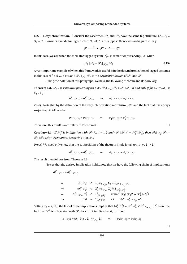
Universally Composing Embedded Systems
6.2.3 Desynchronization. Consider the case when P1 and P2 have the same tag structure, i.e., T1 =T2 =T . Consider a mediator tag structure T ′ of T , i.e., suppose there exists a diagram in Tag:
Tρ - T ′ ρ
T .
In this case, we ask when the mediator tagged system IT ′ is semantics preserving, i.e., when
P1‖P2 ≡P1‖IT ′P2. (6.19)
A very important example of when this framework is useful is in the desynchronization of tagged systems;
in this case T ′ =Ttriv = ∗, and P1‖IT ′P2 is the desynchronization of P1 and P2.
Using the notation of this paragraph, we have the following theorem and its corollary.
Theorem 6.3. IT ′ is semantics preserving w.r.t. I , P1‖IT ′P2 ≡P1‖P2, if and only if for all (σ1,σ2) ∈Σ1 ×Σ2:
σρ1 |V1∩V2 =σ
ρ2 |V1∩V2 ⇒ σ1|V1∩V2 =σ2|V1∩V2 .
Proof. Note that by the definition of the desynchronization morphism ( · )ρ (and the fact that it is always
surjective), it follows that
σ1|V1∩V2 =σ2|V1∩V2 ⇒ σρ1 |V1∩V2 =σ
ρ2 |V1∩V2 .
Therefore, this result is a corollary of Theorem 6.2.
Corollary 6.1. If Pρ
i is in bijection with Pi for i = 1,2 and (P1‖P2)ρ = Pρ1 ‖P
ρ2 , then P1‖IT ′P2 ≡
P1‖P2 (IT ′ is semantics preserving w.r.t. I ).
Proof. We need only show that the suppositions of the theorem imply for all (σ1,σ2) ∈Σ1 ×Σ2
σρ1 |V1∩V2 =σ
ρ2 |V1∩V2 ⇒ σ1|V1∩V2 =σ2|V1∩V2 .
The result then follows from Theorem 6.3.
To see that the desired implication holds, note that we have the following chain of implications:
σρ1 |V1∩V2 =σ
ρ2 |V1∩V2
⇒ (σ1,σ2) ∈ Σ1 ×ΣIT ′ Σ2∼=ΣP1‖IT ′ P2
⇒ (σρ1 ,σρ2 ) ∈ Σρ1 ×ΣIT ′ Σ
ρ2∼=ΣPρ
1 ‖Pρ2
⇒ σρ1 tIT ′ σ
ρ2 ∈ Σ
ρ
P1‖P2(since (P1‖P2)ρ =P
ρ1 ‖P
ρ2 )
⇒ ∃ σ ∈ ΣP1‖P2s.t. σρ =σ
ρ1 tIT ′ σ
ρ2 .
Setting σi = πi (σ), the last of these implications implies that (σρ1 , σρ2 ) = (σρ1 ,σρ2 ) ∈ Σρ1 ×ΣIT ′ Σ
ρ2 . Now, the
fact that Pρ
i is in bijection with Pi for i = 1,2 implies that σi =σi , or:
(σ1,σ2) = (σ1, σ2) ∈Σ1 ×ΣITΣ2 ⇒ σ1|V1∩V2 =σ2|V1∩V2 .
202

Universally Composing Embedded Systems
Example 6.2. We would like to know semantics is preserved by desynchronization for the tagged systems
given in Example 6.1, i.e., for ρ : Tsync →Ttriv the desyncronization morphism, is P1‖P2 ≡P1‖ITtrivP2?
First we apply the necessary and sufficient conditions given in Theorem 6.3. Since V1 ∩V2 = x,
σρ1 (n, x) =σ
ρ2 (n, x) ⇒ σ1(n, x) =σ2(n, x)
σρ1 (n, x) = σ
ρ2 (n, x) ⇒ σ1(n, x) = σ2(n, x)
because σ1(n, x) =σ2(n, x) and σ1(n, x) = σ2(n, x). Therefore, semantics is preserved.
Note that Corollary 6.1 would not tell us whether semantics is preserved, because P2 is not in
bijective correspondence with Pρ2 , and so the conditions of the corollary do not hold. This demonstrates
that Theorem 6.3 is a stronger result than Corollary 6.1.
6.3 Networks of Tagged Systems
In this section, we introduce the notion of a network of tag structures, tagged systems and be-
haviors. Moreover, we are able to show that these objects correspond to networks over the categories Tag,
TagSys and Set, respectively (see Section 1.5). This observation will be fundamental in defining compo-
sition for these networks.
6.3.1 Networks of tag structures. We begin by defining a network of tag structures as in [23] (although
we state the definition in a slightly different manner). A network of tag structures is defined to be a tuple
(Γ,T ,S ,ρ),
where
¦ Γ= (Q,E) is a graph.
¦ T = Tq q∈Q is a set of tag structures.
¦ S = Se e∈E is a set of mediator tag structures, mediating between Tsor(e) and Ttar(e).
¦ ρ= (ρe ,ρ′e )e∈E is a set of pairs of morphisms in Tag, such that for every e ∈ E , there is the following
diagram in Tag:
Tsor(e)ρe - Se
ρ′eTtar(e).
Networks of tagged systems are defined in an analogous manner.
6.3.2 Networks of tagged systems. A network of tagged systems is defined to be a tuple
(Γ,P ,M ,α),
where
203

Universally Composing Embedded Systems
¦ Γ= (Q,E) is a graph.
¦ P = Pq q∈Q is a set of tag structures.
¦ M = Me e∈E is a set of mediator tagged systems, mediating between Psor(e) and Ptar(e).
¦ α = (αe ,α′e )e∈E is a set of pairs of morphisms in TagSys, such that for every e ∈ E , there is the
following diagram in TagSys:
Psor(e)αe- Me
α′e Ptar(e).
Suppose we have a network of tag structures (Γ,T ,S ,ρ) and a collection of tagged systems P = Pq q∈Q
such that Pq has tag structure Tq . Then we can associate to this set of tagged systems a network of tagged
systems, (Γ,P ,IS ,Resρ) with:
IS = ISe e∈E , Resρ = (Resρesor(e),Res
ρ′etar(e))e∈E
where ISe is defined as in (6.6), and Resρesor(e) and Res
ρ′etar(e) are defined as in (6.8), i.e., there is a diagram in
TagSys of the form:
Psor(e)
Resρesor(e)- ISe
Res
ρ′etar(e)
Ptar(e)
for every e ∈ E .
6.3.3 Networks of behaviors. We can define a network of behaviors from the network of tagged sys-
tems, (Γ,P ,M ,α), as a tuple:
(Γ,ΣP ,ΣM ,α),
where
¦ Γ= (Q,E) is a graph.
¦ ΣP = ΣPqq∈Q , where ΣPq
is the set of behaviors for Pq .
¦ ΣM = ΣMee∈E , where ΣMe
is the set of behaviors for Me .
¦ α= (αe ,α′e )e∈E is a set of pairs of morphisms in Set, such that for every e ∈ E , there is the following
diagram in Set:
ΣPsor(e)
αe- ΣMeα′
eΣPtar(e)
.
The association of a network of behaviors from a network of tagged systems can be viewed categorically.
For the network of tagged systems (Γ,P ,M ,α), the functor B : TagSys → Set yields the corresponding
network of behaviors (Γ,ΣP ,ΣM ,α) because
ΣP = ΣPqq∈Q = B(Pq )q∈Q
ΣM = ΣMee∈E = B(Me )e∈E .
204

Universally Composing Embedded Systems
More generally,
ΣPsor(e)
αe- ΣMeα′
eΣPtar(e)
= B
(Psor(e)
αe- Meα′
e Ptar(e)
)for every e ∈ E .
6.3.4 Networks as networks over a category. We define a network of tag structures and a network of
tagged systems to be networks over the categories Tag and TagSys:
T : N→Tag, N : N→TagSys,
where N is an Dop-category. For example, if N is given by the diagram: • −→ •←− •, then the network of
tag structures given in (6.1) and the network of tagged systems given in (6.13) are defined, respectively, by
the functors:
T(• −→•←−•) =(T1
ρ1 - T ρ2T2
), (6.20)
N(• −→•←−•) =(P1
α1- M α2 P2
). (6.21)
More generally, we can associate to a network of tag structures (Γ,T ,S ,ρ) and a network of tagged sys-
tems (Γ,P ,M ,α) functors:
T(T ,S ,ρ) : NΓ →Tag, N(P ,M ,α) : NΓ →TagSys,
where NΓ is the Dop-category associated with Γ, and T(T ,S ,ρ) and N(P ,M ,α) are defined by:
T(T ,S ,ρ) (sor(e) - e tar(e)) := (6.22)(Tsor(e)
ρe - Se ρ′e
Ttar(e)
),
N(P ,M ,α) (sor(e) - e tar(e)) := (6.23)(Psor(e)
αe- Meα′
e Ptar(e)
),
for every e ∈ E .
If (Γ,P ,M ,α) is a network of tagged systems, and (Γ,ΣP ,ΣM ,α) is the associated network of
behaviors, then there is a functor
S(ΣP ,ΣM ,α) : NΓ → Set,
where NΓ is the Dop-category associated with Γ, and S(ΣP ,ΣM ,α) is defined to be the composite:
NΓ
N(P ,M ,α)- TagSysB- Set .
In other words, S(ΣP ,ΣM ,α) is defined by:
S(ΣP ,ΣM ,α) (sor(e) - e tar(e)) :=(ΣPsor(e)
αe- ΣMeα′
eΣPtar(e)
),
= B
(Psor(e)
αe- Meα′
e Ptar(e)
)for every e ∈ E .
205

Universally Composing Embedded Systems
Example 6.3. An example of a network of tagged systems associated to the Dop-category NCk (as intro-
duced in Example 1.24) is given in the following diagram:
Me1
Mek Me2
P1
αe 1
-
α ′
ek
P2
α ′e
1
αe2
-
Pk
α
ek
P3
α′ e 2
-
N(NCk ) = ......
Pi+2 Pi−1
Pi+1 Pi
Mei+1
α
′ e i+1
αe i+1
Mei−1
αe
i−1 -α ′
ei−1-
Mei
α
e i
α ′ei -
6.4 Universally Composing Networks of Tagged Systems
In this section, we give a categorical formulation for composition. Since a network is just a dia-
gram, the composition of a network is the limit of this diagram. To illustrate this concept, we first consider
a network of tag structures and demonstrate how taking the composition of this network is consistent with
the notion of a common tag structure as first introduced in Section 6.1. We then discuss how these ideas
can be generalized to networks of tagged systems. Finally, we explicitly relate the composite of a network
of tagged systems with the composite of a network of behaviors. This relationship will be important when
attempting to prove results relating to semantics preservation.
6.4.1 Composing networks of tag structures. Recall that for two tag structures, T1 and T2, communi-
cating through a mediator tag structure, T , we obtained a single, common, tag structure that was unique
up to isomorphism; the common tag structure, T1 ×T T2, was the pullback of the diagram given in (6.1).
But the pullback is just a special case of the limit of a functor (see Appendix A), i.e.,
T1 ×T T2 = Lim(•−→•←−•)(T) = Lim(•−→•←−•)
(T1
ρ1 - T ρ2T2
),
where T : (• −→•←−•) →Tag is defined as in (6.20).
Therefore, we can define a tag structure common to an entire network of tag structures by tak-
ing the limit (defined in Appendix A) of the corresponding diagram in Tag describing this network. If
(Γ,T ,S ,ρ) is a network of tag structures and
T(T ,S ,ρ) : NΓ →Tag
206
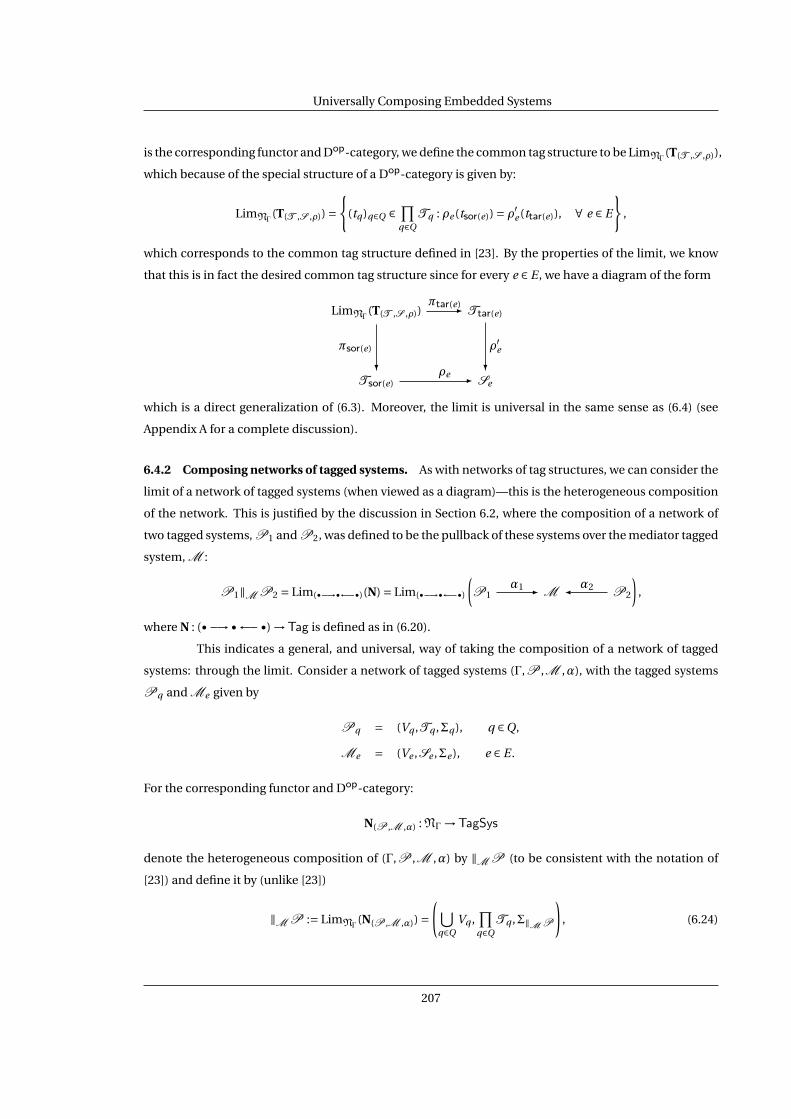
Universally Composing Embedded Systems
is the corresponding functor and Dop-category, we define the common tag structure to be LimNΓ(T(T ,S ,ρ)),
which because of the special structure of a Dop-category is given by:
LimNΓ(T(T ,S ,ρ)) =
(tq )q∈Q ∈ ∏
q∈QTq : ρe (tsor(e)) = ρ′e (ttar(e)), ∀ e ∈ E
,
which corresponds to the common tag structure defined in [23]. By the properties of the limit, we know
that this is in fact the desired common tag structure since for every e ∈ E , we have a diagram of the form
LimNΓ(T(T ,S ,ρ))
πtar(e)- Ttar(e)
Tsor(e)
πsor(e)
? ρe - Se
ρ′e?
which is a direct generalization of (6.3). Moreover, the limit is universal in the same sense as (6.4) (see
Appendix A for a complete discussion).
6.4.2 Composing networks of tagged systems. As with networks of tag structures, we can consider the
limit of a network of tagged systems (when viewed as a diagram)—this is the heterogeneous composition
of the network. This is justified by the discussion in Section 6.2, where the composition of a network of
two tagged systems, P1 and P2, was defined to be the pullback of these systems over the mediator tagged
system, M :
P1‖M P2 = Lim(•−→•←−•)(N) = Lim(•−→•←−•)
(P1
α1- M α2 P2
),
where N : (• −→•←−•) →Tag is defined as in (6.20).
This indicates a general, and universal, way of taking the composition of a network of tagged
systems: through the limit. Consider a network of tagged systems (Γ,P ,M ,α), with the tagged systems
Pq and Me given by
Pq = (Vq ,Tq ,Σq ), q ∈Q,
Me = (Ve ,Se ,Σe ), e ∈ E .
For the corresponding functor and Dop-category:
N(P ,M ,α) : NΓ →TagSys
denote the heterogeneous composition of (Γ,P ,M ,α) by ‖M P (to be consistent with the notation of
[23]) and define it by (unlike [23])
‖M P := LimNΓ(N(P ,M ,α)) =
( ⋃q∈Q
Vq ,∏
q∈QTq ,Σ‖MP
), (6.24)
207

Universally Composing Embedded Systems
where Σ‖MP is the set of behaviors
σ :N× ⋃q∈Q
Vq → ∏q∈Q
Tq ×D
σ(n, v) 7→ ((tq )q∈Q , d
)such that the following conditions hold: for all (n, v) ∈N×⋃
q∈Q Vq , there exists unique (σq )q∈Q ∈∏q∈Q Σq
such that2 for all e ∈ E
σ(n, v) = ((tq )q∈Q , d
) ⇔
(i′) σsor(e)(n, v) = (tsor(e), d) if v ∈ Vsor(e)
and
(ii′) σtar(e)(n, v) = (ttar(e), d) if v ∈ Vtar(e)
and
(iii′) αe (σsor(e))(n, w) =α′e (σtar(e))(n, w)
∀ w ∈ Ve .
(6.25)
Because σ ∈ Σ‖MP is uniquely determined by (σq )q∈Q ∈ ∏q∈Q Σq satisfying the right-hand side of (6.25),
we write
σ=⊔M
(σq )q∈Q ∈Σ‖MP
for the corresponding element on the left-hand side of (6.25), and call it the unification of (σq )q∈Q ∈∏q∈Q Σq . Conversely, every element of Σ‖MP can be written as the unification of an element of
∏q∈Q Σq ,
so there are projection maps πq , q ∈Q, given by
πq : Σ‖MP → Σq
σ=⊔M
(σq )q∈Q 7→ σq =πq (σ).
We can obtain a better understanding of the behaviors of the tagged system ‖M P by consider-
ing the associated network of behaviors.
6.4.3 Composing networks of behaviors. Let (Γ,P ,M ,α) be a network of tagged systems, (Γ,ΣP ,ΣM ,α)
the associated network of behaviors, and
S(ΣP ,ΣM ,α) = B N(P ,M ,α) : NΓ → Set,
the associated functor and Dop-category. Because of the special structure of an Dop-category, we can
explicitly compute the limit of the functor S(ΣP ,ΣM ,α); it is given by
LimNΓ(S(ΣP ,ΣM ,α)) = (6.26)
(σq )q∈Q ∈ ∏q∈Q
Σq :αe (σsor(e)) =α′e (σtar(e)), ∀ e ∈ E
.
2Unlike (6.5), the third condition stated here is no longer redundant.
208

Universally Composing Embedded Systems
Now, there is a bijection:
Σ‖MP∼= LimNΓ
(S(ΣP ,ΣM ,α)). (6.27)
The map from Σ‖MP to LimNΓ(S(ΣP ,ΣM ,α)) is given by
(πq )q∈Q : Σ‖MP∼−→ LimNΓ
(S(ΣP ,ΣM ,α)) (6.28)
σ 7→ (πq (σ))q∈Q .
The inverse of this map is given by the unification operator generalized to the network case. That is⊔M
( · ) : LimNΓ(S(ΣP ,ΣM ,α))
∼−→ Σ‖MP (6.29)
(σq )q∈Q 7→ σ=⊔M
(σq )q∈Q ,
where σ is given as in the left-hand side of equation (6.25), which is well defined because of the definition
of LimNΓ(S(ΣP ,ΣM ,α)), i.e., because an element (σq )q∈Q ∈ LimNΓ
(S(ΣP ,ΣM ,α)) automatically satisfies the
right-hand side of (6.25) by (6.26).
6.4.4 Composition over identity mediator tagged systems. An especially interesting case is when the
network of tagged systems is obtained from a network of tag structures (Γ,T ,S ,ρ), i.e., the network of
tagged systems is given by (Γ,P ,IS ,Resρ). Here we explicitly carry out the construction of ‖ISP , and
demonstrate how this yields the correct definition of ‖ISP so as to be consistent with [23].
If Pq = (Vq ,Tq ,Σq ) for all q ∈Q, then
‖ISP = LimNΓ
(N(P ,IS ,Resρ)) =( ⋃
q∈QVq ,LimNΓ
(T(T ,S ,ρ)),Σ‖ISP
),
where Σ‖ISP is defined in the same way as Σ‖MP with the appropriate modifications, i.e., Σ‖IS
P is the
set of behaviors
σ :N× ⋃q∈Q
Vq → LimNΓ(T(T ,S ,ρ))×D ⊂ ∏
q∈QTq ×D
σ(n, v) 7→ ((tq )q∈Q , d
),
such that the following conditions hold: for all (n, v) ∈N×⋃q∈Q Vq , there exists unique (σq )q∈Q ∈∏
q∈Q Σq
such that3 for all e ∈ E
σ(n, v) = ((tq )q∈Q , d
) ⇔
(i′′) σsor(e)(n, v) = (tsor(e), d) if v ∈ Vsor(e)
and
(ii′′) σtar(e)(n, v) = (ttar(e), d) if v ∈ Vtar(e)
and
(iii′′) σρesor(e)|Vsor(e)∩Vtar(e) =σ
ρ′etar(e)|Vsor(e)∩Vtar(e) .
(6.30)
3Like (6.5) and unlike (6.25), the third condition stated here is again redundant because we are taking LimNΓ(T(T ,S ,ρ)) as our
tag structure.
209

Universally Composing Embedded Systems
Note that the fact thatσ ∈Σ‖ISP takes values in LimNΓ
(T(T ,S ,ρ)), rather than∏
q∈Q Tq , is exactly because
of condition (iii′′).
The conditions given in (6.30) demonstrate that our definition of Σ‖ISP is consistent with the
one given in [23] (although our definition of Σ‖MP is more general that anything defined in that chapter).
Moreover, (6.26), (6.27) and (6.30) imply that we have the following bijection
Σ‖ISP
∼= LimNΓ(S(ΣP ,ΣIS
,Resρ)) (6.31)
=
(σq )q∈Q ∈ ∏q∈Q
Σq :σρesor(e)|Vsor(e)∩Vtar(e) =σ
ρ′etar(e)|Vsor(e)∩Vtar(e) , ∀ e ∈ E
as defined in (6.28) and (6.29). Here
S(ΣP ,ΣIS,Resρ) = B N(P ,IS ,Resρ) : NΓ → Set
is the functor corresponding to the network of behaviors (Γ,ΣP ,ΣIS,Resρ) obtained from the network of
tagged systems (Γ,P , IS ,Resρ).
6.5 Semantics Preserving Deployments of Networks
Using the framework established in this chapter, we are able to introduce a general notion of
semantics preservation. After this concept is introduced, we state the main result of this work: necessary
and sufficient conditions for semantics preservation. We conclude this section by applying this result to
the specific case of network desyncronization.
6.5.1 Network specification vs. network deployment. Generalizing the notion of specification vs. de-
ployment given in Section 6.2, we define the following semantics (using the notation of the previous para-
graph):
Network Specification Semantics: ‖ISP
Network Deployment Semantics: ‖M P
The set of mediator tagged systems M is said to be semantics preserving with respect to IS , denoted by
‖M P ≡ ‖ISP
if for all (σq )q∈Q ∈∏q∈Q Σq
∃ σ′ ∈Σ‖MP s.t. πq (σ′) =σq ∀ q ∈Q
m∃ σ ∈Σ‖IS
P s.t. πq (σ) =σq ∀ q ∈Q.
(6.32)
We now are able to generalize the results given in Theorem 6.2 on semantics preservation to the networks
of tagged systems case.
210

Universally Composing Embedded Systems
Theorem 6.4. For the networks, (Γ,P ,M ,α) and (Γ,P ,IS ,Resρ),
‖M P ≡ ‖ISP
if and only if for all (σq )q∈Q ∈∏q∈Q Σq and all e ∈ E:
αe (σsor(e)) =α′e (σtar(e)) ⇔ Resρe
sor(e)(σsor(e)) = Resρ′etar(e)(σtar(e)).
Proof. (Sufficiency:) If
(σq )q∈Q ∈ ∏q∈Q
Σq s.t. αe (σsor(e)) =α′e (σtar(e)) ∀ e ∈ E
by (6.26)⇒ (σq )q∈Q ∈ LimNΓ(S(ΣP ,ΣM ,α))
by (6.29)⇒ ⊔M (σq )q∈Q ∈Σ‖MP where
πq(⊔
M (σq )q∈Q)=σq ∀ q ∈Q
by (6.32)⇒ ∃ σ ∈Σ‖ISP s.t. πq (σ) =σq ∀ q ∈Q
by (6.28)⇒ (σq )q∈Q ∈ LimNΓ(S(ΣP ,ΣIS
,Resρ))by (6.31)⇒ Resρe
sor(e)(σsor(e)) = Resρ′etar(e)(σtar(e)) ∀ e ∈ E .
The converse direction proceeds in the same manner: if
(σq )q∈Q ∈ ∏q∈Q
Σq s.t. Resρesor(e)(σsor(e)) = Res
ρ′etar(e)(σtar(e)) ∀ e ∈ E
by (6.29)⇒ ⊔IS
(σq )q∈Q ∈Σ‖ISP where
πq(⊔
IS(σq )q∈Q
)=σq ∀ q ∈Qby (6.32)⇒ ∃ σ′ ∈Σ‖MP s.t. πq (σ′) =σq ∀ q ∈Qby (6.28)⇒ (σq )q∈Q ∈ LimNΓ
(S(ΣP ,ΣM ,α))by (6.26)⇒ αe (σsor(e)) =α′
e (σtar(e)) ∀ e ∈ E .
(Necessity:) We have the following implications:
∃ σ′ ∈Σ‖MP s.t. πq (σ′) =σq ∀ q ∈Q
by (6.28)⇒ (σq )q∈Q ∈ LimNΓ(S(ΣP ,ΣM ,α))
by (6.26)⇒ αe (σsor(e)) =α′e (σtar(e)) ∀ e ∈ E
⇒ Resρesor(e)(σsor(e)) = Res
ρ′etar(e)(σtar(e)) ∀ e ∈ E
by (6.29)⇒ ⊔IS
(σq )q∈Q ∈Σ‖ISP and
πq(⊔
IS(σq )q∈Q
)=σq ∀ q ∈Q.
Therefore⊔
IS(σq )q∈Q is the element of Σ‖IS
P such that πq(⊔
IS(σq )q∈Q
)=σq for all q ∈Q.
211

Universally Composing Embedded Systems
The other direction follows in the same way:
∃ σ ∈Σ‖ISP s.t. πq (σ) =σq ∀ q ∈Q
⇒ ⊔M (σq )q∈Q ∈Σ‖MP and
πq(⊔
M (σq )q∈Q)=σq ∀ q ∈Q,
by (6.26), (6.28) and (6.29), so⊔
M (σq )q∈Q is the element of Σ‖MP such that
πq
(⊔M
(σq )q∈Q
)=σq
for all q ∈Q.
6.5.2 Network desyncronization. Let T and T ′ be two tag structures and ρ : T →T ′ be a morphism
between these tag structures. By slight abuse of notation, let (Γ,T ,T ′,ρ) denote the network of tag struc-
tures such that Tq = T for all q ∈ Q and T ′e = T ′, ρe = ρ′e = ρ for all e ∈ E ; denote the corresponding
network of tagged systems by (Γ,P ,IT ′ ,Resρ). Similarly, let (Γ,T ,T , id) denote the network of tag struc-
tures with Tsor(e) = Ttar(e) = Te = T for all e ∈ E , and with all morphisms of tag structures being the
identity; denote the corresponding network of tagged systems by (Γ,P ,I ,Resid). Therefore, this network
consists of a set of tagged systems, all with the same tag structure, communicating through the identity
tagged system. A special case in which this framework in interesting is when T ′ =Ttriv = ∗; in this case
(Γ,P ,IT ′ ,Resρ) is the desynchronization of (Γ,P ,I ,Resid).
Utilizing the notation of Section 6.4, and generalizing the discussion on desynchronization given
in this Section 6.2, we are interested in when
‖P := LimNΓ(N(T ,T ,id)) ≡ LimNΓ
(N(T ,T ′,ρ)) =: ‖IT ′P .
In other words, we would like to know when IT ′ is semantics preserving. The following corollary (of
Theorem 6.4) says that this happens exactly when every element of IT ′ is semantics preserving.
Corollary 6.2. IT ′ is semantics preserving, ‖P ≡ ‖IT ′P , if and only if for all (σq )q∈Q ∈ ∏q∈Q Σq and all
e ∈ E:
σρ
sor(e)|Vsor(e)∩Vtar(e) =σρ
tar(e)|Vsor(e)∩Vtar(e) ⇒ σsor(e)|Vsor(e)∩Vtar(e) =σtar(e)|Vsor(e)∩Vtar(e) .
212

Appendix A
Limits
Central to category theory, and hence to all of mathematics, is the notion of a universal prop-
erty, which characterizes objects that share a certain property, i.e., objects displaying such a property are
unique up to isomorphism. Examples abound in category theory (e.g., products and limits) but also ap-
pear in engineering, although almost never recognized (e.g., stability is a universal property).
This appendix reviews some of the most fundamental universal constructions in a category:
products, equalizers, pullbacks and limits. This is done in order to provide the necessary preliminaries for
Chapter 6.
A.1 Products
A.1.1 Binary products. Let C be a category and A and B two objects in C. The product of these objects,
if it exists, is an object C = A×B of C together with a pair of morphisms pA : A×B → A and pB : A×B → B
(called projections). It must satisfy the universal property that for any other object D of C together with
a pair of morphisms f : D → A and g : D → B, there exists a unique morphism h : D → A×B making the
following diagram:
D
A pA
f
A×B
h
? pB - B
g
-
commute. The morphism h is typically denoted by ( f , g ).
Example A.1. For two sets A and B, the binary product of these sets is the usual cartesian product:
A×B = (a, b) : a ∈ A and b ∈ B.
213

Limits
A.1.2 Products. Let C be a category, I be a set and Ai i∈I a set of objects of C. The product of these ob-
jects is an object∏
i∈I Ai of C together with projections pAi :∏
i∈I Ai → Ai satisfying the universal property
that for any other object C of C with morphisms fi : C → Ai , there exists a unique morphism
( fi )i∈I : C →∏i∈I
Ai
making the following diagram
C
AipAi
fi
∏i∈I
Ai
( fi )i∈I
?
commute for all i ∈ I .
Given two sets of objects Ai i∈I and Bi i∈I together with morphisms fi : Ai → Bi , there is a
unique induced morphism ∏i∈I
fi = ( fi pAi )i∈I :∏i∈I
Ai →∏i∈I
Bi
making the following diagram
AipAi
∏i∈I
Ai
Bi
fi
?pBi
∏i∈I
Bi
∏i∈I fi = ( fi pAi )i∈I
?
commute.
Definition A.1. A category C is said to have products, or products exist in C, if for any set of objects Ai i∈I
in C, the product∏
i∈I Ai exists.
Remark A.1. Products of the form given in Definition A.1 are often referred to as small products. Some-
times finite products—I is a finite set—are often of interest.
Example A.2. The category of sets, Set, has products. For a set of sets Xi i∈I , the product is the usual
cartesian product: ∏i∈I
Xi = (xi )i∈I : xi ∈ Xi .
The projections are defined as
pi :∏i∈I
Xi → Xi
(xi )i∈I 7→ xi .
To verify the universal property of the product, consider a set D and functions fi : D → Xi . From these we
obtain a function f : D →∏i∈I Xi given by:
f (y) = ( fi (y))i∈I
214

Limits
for all y ∈ D.
A.1.3 Products of graphs. The category of graphs, Grph, has products. For a set of graphs Γi = (Qi ,Ei )i∈I ,
the product is induced from the product on sets as follows:
∏i∈I
Γi = (∏i∈I
Qi ,∏i∈I
Ei ).
The source and target maps for the product graph∏
i∈I Γi are defined to be the unique maps making the
following diagrams commute:
Ei pEi
∏i∈I
Ei
Qi
sori
?pQi
∏i∈I
Qi
∏i∈I sori
?
Ei pEi
∏i∈I
Ei
Qi
tari
?pQi
∏i∈I
Qi
∏i∈I tari
?
Specifically, for (ei )i∈I ∈∏i∈I Ei ,
∏i∈I
sori ((ei )i∈I ) = (sori (ei ))i∈I ,∏i∈I
tari ((ei )i∈I ) = (tari (ei ))i∈I .
Note that the projections are defined by:
pΓi := (pEi , pQi ) :∐i∈I
Γi → Γi .
Finally, we must verify the universal property of the product. Consider a graph Γ = (Q,E) together with
a collection of morphisms Fi = ((FQ)i , (FE )i ) : Γ→ Γi . It follows from the universality of products in the
category of sets that the diagrams given in Table A.1 are commutative. So F = (FQ ,FE ) : Γ→ ∏i∈I Γi is the
desired unique morphism.
A.1.4 Products in categories of hybrid objects. The existence of products in C relates to the existence
of products in Hy(C). In order to establish this relationship, we need to show that products exist in Dcat
and that if products exist for C then they exist for CJ for any small category J. These two results are then
“glued” together to yield products in Hy(C).
Proposition A.1. Products exist in Dcat. Specifically, for Ai i∈I a set of D-categories, the product∏
i∈I Ai
exists and is given by: ∏i∈I
Ai = dcat(∏i∈I
grph(Ai )),
where∏
i∈I grph(Ai ) is the product of graphs.
Proof. This follows from the fact that dcat and grph are isomorphisms between categories (Theorem 1.1).
Specifically, the projections:
Pi :∏i∈I
grph(Ai ) → grph(Ai )
215

Limits
E
Q
sor
-
∏i∈I
Ei
FQ
?
Ei
(FE
) i
pE i
∏i∈I
Qi
FE
?
∏i∈I sori
-
Qi
(FQ
) i
sori-
pQ i
E
Q
tar
-
∏i∈I
Ei
FQ
?
Ei
(FE
) i
pE i
∏i∈I
Qi
FE
?
∏i∈I tari
-
Qi
(F
Q) i
tari-
pQ i
Table A.1: Commuting diagrams verifying the universality of the product in Grph.
yield projections of D-categories:
~Pi := dcat(Pi ) :∏i∈I
Ai = dcat(∏i∈I
grph(Ai )) →Ai = dcat(grph(Ai )).
Now, to verify universality, for any other D-category D with morphisms ~Fi : D → Ai there is a graph
grph(D) and morphisms grph(~Fi ) : grph(D) → grph(Ai ). By the universality of the product in Grph, there
exists a unique morphism F making the following diagram
grph(D)
grph(Ai ) Pi
grph(~Fi )
∏i∈I
grph(Ai )
F
?
216

Limits
commute. Applying the functor dcat yields a commuting diagram
D
Ai
~Pi
~Fi
∏i∈I
Ai
dcat(F )
?
where dcat(F ) must be unique; if there were another morphisms making the diagram commute, it would
also make the corresponding diagram of graphs commute, thus violating the uniqueness of F .
Lemma A.1. If products exist in C, then products exists in CJ for any small category J. Specifically, for a set
of functors Fi : J→C, i ∈ I, the product is given on objects and morphisms by:
(∏i∈I
Fi )(a) =∏i∈I
Fi (a), (∏i∈I
Fi )(α) =∏i∈I
Fi (α).
Proof. See [74], Theorem 1, page 115.
Proposition A.2. If products exist in C, then products exist in Hy(C). Specifically, for a set of hybrid objects
(Ai ,Ai )i∈I , the product is given by:
∏i∈I
(Ai ,Ai ) = (∏i∈I
Ai ,∏i∈I
~P∗i (Ai ))
where∏
i∈I Ai is the product of D-categories,∏
i∈I ~P∗i (Ai ) is the product in C
∏i∈I Ai with ~Pi :
∏i∈I Ai → Ai
the projection morphisms in Dcat.
Proof. The projection morphisms are given by:
(~Pi , ~pi ) :∏i∈I
(Ai ,Ai ) → (Ai ,Ai ),
where ~Pi :∏
i∈I Ai →Ai and
~pi :∏i∈I
~P∗i (Ai )
→ ~P∗i (Ai )
is objectwise the projection in C. We must verify the universality of the product. Consider a hybrid object
(D,D) together with morphisms (~Fi , ~fi ) : (D,D) → (Ai ,Ai ). By the universality of the product in Dcat, there
exists a unique morphism ~F : D →∏i∈I Ai yielding a commuting diagram
D
Ai
~Pi
~Fi
∏i∈I
Ai
~F
?
217
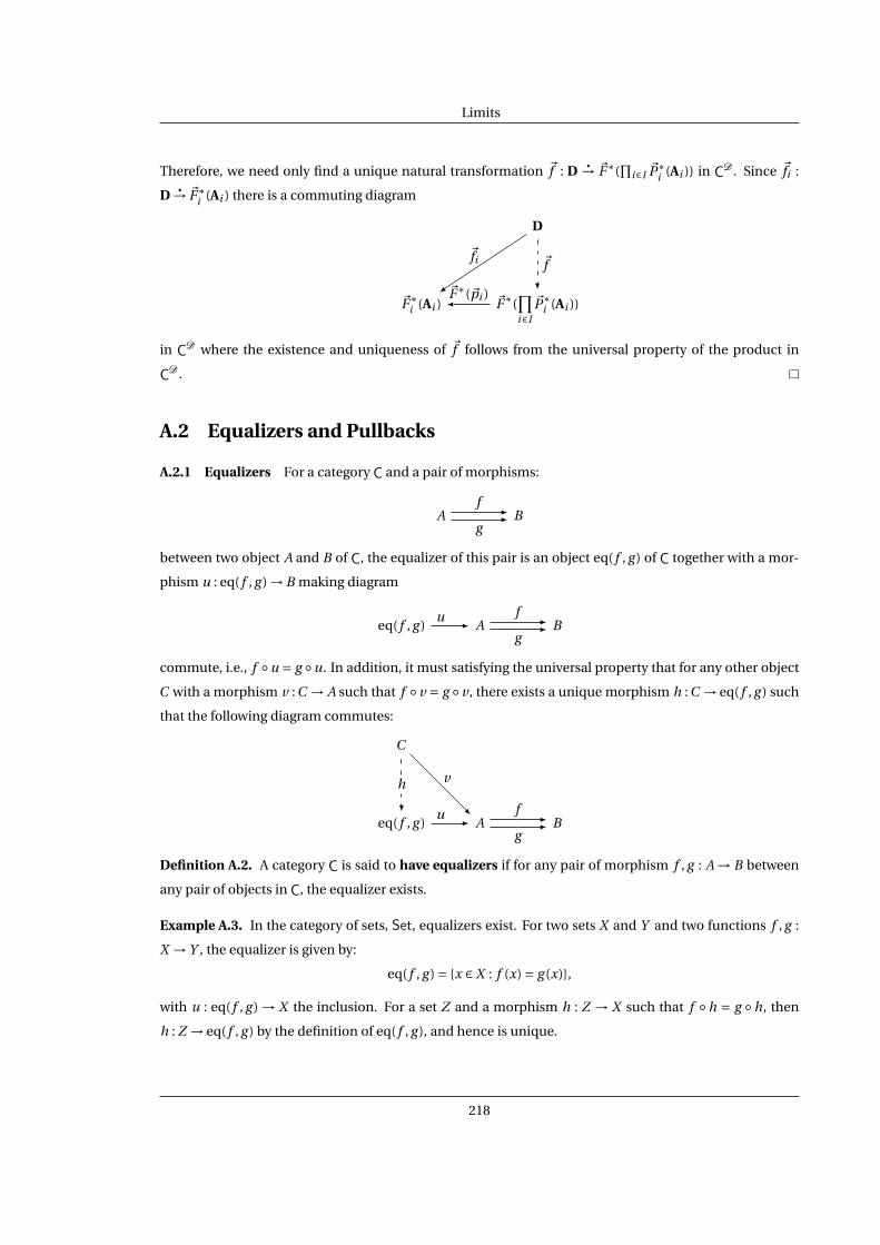
Limits
Therefore, we need only find a unique natural transformation ~f : D→ ~F∗(
∏i∈I ~P
∗i (Ai )) in CD . Since ~fi :
D→ ~F∗
i (Ai ) there is a commuting diagram
D
~F∗i (Ai )
~F∗(~pi )
~fi
~F∗(
∏i∈I
~P∗i (Ai ))
~f
?
in CD where the existence and uniqueness of ~f follows from the universal property of the product in
CD .
A.2 Equalizers and Pullbacks
A.2.1 Equalizers For a category C and a pair of morphisms:
Af -
g- B
between two object A and B of C, the equalizer of this pair is an object eq( f , g ) of C together with a mor-
phism u : eq( f , g ) → B making diagram
eq( f , g )u - A
f -
g- B
commute, i.e., f u = g u. In addition, it must satisfying the universal property that for any other object
C with a morphism v : C → A such that f v = g v, there exists a unique morphism h : C → eq( f , g ) such
that the following diagram commutes:
C
eq( f , g )
h
? u - Af -
g-
v
-
B
Definition A.2. A category C is said to have equalizers if for any pair of morphism f , g : A → B between
any pair of objects in C, the equalizer exists.
Example A.3. In the category of sets, Set, equalizers exist. For two sets X and Y and two functions f , g :
X → Y , the equalizer is given by:
eq( f , g ) = x ∈ X : f (x) = g (x),
with u : eq( f , g ) → X the inclusion. For a set Z and a morphism h : Z → X such that f h = g h, then
h : Z → eq( f , g ) by the definition of eq( f , g ), and hence is unique.
218

Limits
A.2.2 Equalizers in Grph. For a diagram in Grph of the form:
Γ= (Q,E)F = (FQ ,FE )-
G = (GQ ,GE )- Γ′ = (Q′,E ′),
the equalizer of this pair of morphisms exists. It is given by:
eq(F,Q) = (eq(FQ ,GQ),eq(FE ,GE )),
where the equalizers on the right are in the category of sets. The source and target functions for eq(F,G)
are given uniquely by requiring that the following diagrams commute:
eq(FE ,GE )uE - E
FE -
GE
- E ′
eq(FQ ,GQ)
soreq(F,G)
? uQ - E
sor
? FQ -
GQ
- Q′
sor′
?
eq(FE ,GE )uE - E
FE -
GE
- E ′
eq(FQ ,GQ)
tareq(F,G)
? uQ - E
tar
? FQ -
GQ
- Q′
tar′
?
Note that the uniqueness of the source and target functions are due to the universality of equalizers in
Set. It also follows from the definition of equalizers in Set that
soreq(F,G) = sor |eq(FE ,GE ), tareq(F,G) = tar |eq(FE ,GE ),
since uE and uQ are inclusions.
The universality of the equalizer in Grph is easy to verify (it is a simple exercise in diagram chas-
ing).
A.2.3 Pullbacks. Consider a category C and a diagram of the form:
B
Cg
- A
f
?
The pullback of this diagram is an object B ×A C of C together with two morphisms p and q such that the
following diagram
B ×A Cp - B
C
q
?
g- A
f
?
219

Limits
commutes. It is universal in the following sense: for any other object D of C with morphisms u and v
making the following diagram commute
Du - B
C
v
?
g- A
f
?
there exists a unique morphism h : D → B ×A C such that the following diagram commutes:
D
B ×A Cp
-
h
-
B
u
-
C
q
?
g-
v
-
A
f
?
Pullbacks are very useful when dealing with networks over a category since the canonical Dop-category is
of the form:
b
cta
- a
sa
?
Example A.4. In the category of sets, pullbacks exists. Specifically, for a diagram of sets of the form:
X
Yg
- Z
f
?
The pullback is given by:
X ×Z Y = (x, y) ∈ X ×Y : f (x) = g (y).
A.3 Limits
A.3.1 Limits For a category C and a functor D : J→C the limit, if it exists, is an object of C, denoted by
LimJ(D), together with morphisms:
νa : LimJ(D) → D(a), a ∈Ob(J),
220

Limits
such that for every α : a → b in J, the following diagram
LimJ(D)
D(a)D(α) -
νa
D(b)
νb
-
commutes. In addition it is required to satisfy the universal property that for any object C of C with mor-
phisms ca : C → D(a), a ∈Ob(J), such that there is a commuting diagram:
C
D(a)D(α) -
ca
D(b)
cb
-
there exists a unique morphism u : C → LimJ(D) making the following diagram
C
LimJ(D)
u
?
D(a)D(α) -
ca
νa
D(b)
cb
-νb -
commute.
The notion of a limit perhaps can be better understood utilizing the language of natural trans-
formations. For the constant functor ∆J : C→CJ, the limit of D is an object LimJ(D) of C together with a
universal natural transformation:
ν : ∆J(LimJ(D))→ D.
It must be universal in the following sense: for any other object C of C and natural transformation c :
∆J(C )→ D, there exists a unique morphism u : C → LimJ(D) such that the following diagram commutes
∆J(C )
∆J(LimJ(D))
∆J(u)
?ν - D
c
-
in CJ.
Definition A.3. A category C is complete if for every small category J and every functor D : J → C, the
limit exists.
Example A.5. The category of sets, Set, is the canonical example of a complete category.
221

Limits
The category of small categories Cat is complete; this completeness is directly a result of the
completeness of Set. In fact, one might be tempted to say that the category of D-categories is complete
since the category of small categories is complete. The problem with this logic is that there is no guarantee
that the limit of diagram in Dcat is again in Dcat.
Another example of a complete category is the category of graphs, Grph, which is again complete
because the category of sets is complete. It turns out that the completeness of this category does imply
the completeness of Dcat, which is not surprising in light of the isomorphism Dcat∼=Grph.
A.3.2 Special cases of the limit. The limit includes as a special case all of the previous universal con-
structions we have introduced. Specifically,
Products. The limit of a functorD : I→C,
where I is the discrete category obtained from an indexing set I .Equalizers. The limit of a functor
D : (•→→•) →C .
Pullback. The limit of a functorD : (•→•←•) →C .
Interestingly enough, the existence of limits in a category is related to the existence of equalizers and
products.
Proposition A.3. A category C is complete iff it has equalizers and products.
Proof. See Corollary 2, page 113, [74].
Corollary A.1. The category of graphs, Grph, is complete.
A corollary of this is that the category of D-categories is complete. Before stating this result, we
introduce some notation.
Notation A.1. To differentiate, when necessary, between limits in different categories, we sometimes write
LimCJ
for the limit of a functor D : J→C. Similarly, we sometimes write ∆CJ
.
Theorem A.1. The category of D-categories, Dcat, is complete. Specifically, for a functor D : J → Dcat, J
small, the limit is given by:
LimDcatJ (D) = dcat
(LimGrph
J(grph∗(D))
).
Proof. Follows from the fact that dcat and grph are isomorphisms of categories; the proof is analogous to
the proof of Proposition A.1.
222

Limits
A.3.3 The limit as a functor. If C is a complete category, then the limit exists for every diagram over a
small category J, i.e., for every functor D : J→C. In fact, the universality of the limit implies that it defines
a functor
LimJ : CJ →C .
Specifically, consider two functors D,D′ : J → C together with the corresponding universal natural trans-
formations:
ν : ∆J(LimJ(D))→ D,
ν′ : ∆J(LimJ(D′))→ D′.
The object function of the limit (as a functor) associates to these functors their limit. For a morphism
f : D→ D′, the limit of this morphism is the unique morphism LimJ( f ) : LimJ(D) → LimJ(D′) making the
following diagram:
∆J(LimJ(D))ν - D
∆J(LimJ(D′))
∆J(LimJ( f ))
?ν′ - D′
f
?
commute.
An especially useful result is outlined in the following proposition (see [74], Theorem 1, page
115).
Proposition A.4. If C is complete, then CK is complete for every small category K. Specifically, for D : J →CK, the limit is given on objects and morphisms of K by:
LimCK
J(D)(a) = LimC
K(D(a)), LimCK
J(D)(α) = LimC
K(D(α)).
A.4 Limits in Categories of Hybrid Objects
As an application of these ideas, we will prove that if C is complete, then Hy(C) is complete.
This result was established in [6]; in addition, it was proven that if C is cocomplete (the dual notion to
completeness) then Hy(C) is complete.
A.4.1 Diagrams in categories of hybrid objects. By slight abuse of notation, we denote a diagram in
Hy(C) by
(DJ,DJ) : J→Hy(C).
That is, for every α : a → b in J, there are corresponding hybrid objects and morphisms:
(DJ(a),DJ(a))(DJ(α),DJ(α))- (DJ(b),DJ(b)).
223

Limits
In particular, DJ(α) : DJ(a) →DJ(b) is a morphism of D-categories and
DJ(α) : DJ(a)→ (DJ(α))∗(DJ(b))
is a morphism in CDJ(a).
Note that by the definition of a hybrid object, we can without ambiguity write DJ : J → Dcat;
note that DJ is not a D-category, but a diagram of such categories. Since the category of D-categories is
complete, there exists a D-category LimDcatJ
(DJ) together with a universal natural transformation:
~V : ∆DcatJ (LimDcat
J (DJ))→DJ.
The motivation for denoting this natural transformation by ~V is that for every diagram of the form α : a →b in J, there is a diagram of D-categories:
LimDcatJ (DJ)
DJ(a)DJ(α) -
~Va
DJ(b)
~Vb
-(A.1)
For the diagram (DJ,DJ) : J→Hy(C) in Hy(C), the limit of DJ : J→Dcat yields a functor:
~V ∗(DJ) : J→CLimDcatJ (DJ)
defined on objects and morphisms of J by:
~V ∗(DJ)(a) := ~V ∗a (DJ(a)), ~V ∗(DJ)(α) := ~V ∗
dom(α)(DJ(α)).
Note that ~V ∗(DJ) is well-defined because of the commutativity of (A.1).
Using this notation, we can now prove that categories of hybrid objects are complete and give
an explicit formula for the limit of a diagram.
Theorem A.2. If C is complete, then Hy(C) is complete. Specifically, for (DJ,DJ) : J → Hy(C), the limit is
given by:
LimHy(C)J
(DJ,DJ) =(LimDcat
J (DJ),LimCLimDcat
J(DJ)
J(~V ∗(DJ))
).
Proof. The first step is to find the universal natural transformation in Hy(C)J
ν : ∆Hy(C)J
(LimHy(C)
J(DJ,DJ)
)→ (DJ,DJ).
There are universal natural transformations
~V : ∆DcatJ
(LimDcat
J (DJ))
→ DJ
~ν : ∆CLimDcat
J(DJ)
J
(LimC
LimDcatJ
(DJ)
J(~V ∗(DJ))
)→ ~V ∗(DJ)
in DcatJ and (CLimDcatJ (DJ))J.
224
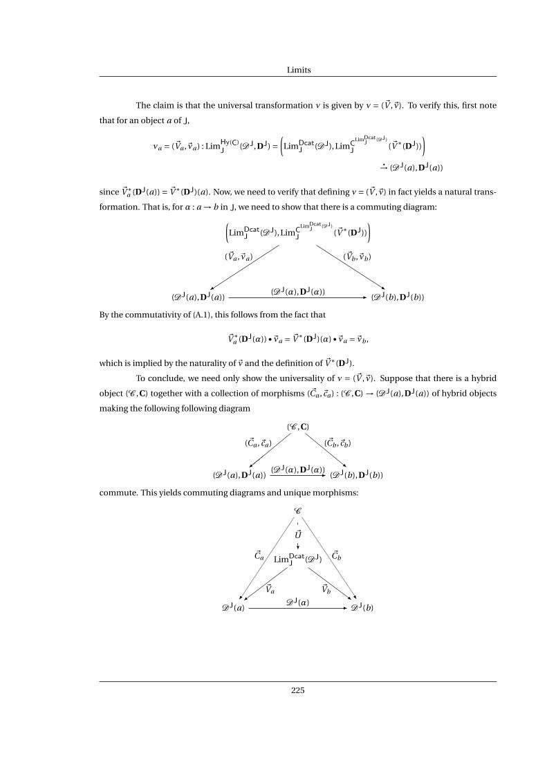
Limits
The claim is that the universal transformation ν is given by ν = (~V ,~ν). To verify this, first note
that for an object a of J,
νa = (~Va ,~νa) : LimHy(C)J
(DJ,DJ) =(LimDcat
J (DJ),LimCLimDcat
J(DJ)
J(~V ∗(DJ))
)→ (DJ(a),DJ(a))
since ~V ∗a (DJ(a)) = ~V ∗(DJ)(a). Now, we need to verify that defining ν= (~V ,~ν) in fact yields a natural trans-
formation. That is, for α : a → b in J, we need to show that there is a commuting diagram:(LimDcat
J (DJ),LimCLimDcat
J(DJ)
J(~V ∗(DJ))
)
(DJ(a),DJ(a))(DJ(α),DJ(α)) -
(~Va ,~νa)
(DJ(b),DJ(b))
(~Vb ,~νb)
-
By the commutativity of (A.1), this follows from the fact that
~V ∗a (DJ(α))•~νa = ~V ∗(DJ)(α)•~νa =~νb ,
which is implied by the naturality of ~ν and the definition of ~V ∗(DJ).
To conclude, we need only show the universality of ν = (~V ,~ν). Suppose that there is a hybrid
object (C ,C) together with a collection of morphisms (~Ca ,~ca) : (C ,C) → (DJ(a),DJ(a)) of hybrid objects
making the following following diagram
(C ,C)
(DJ(a),DJ(a))(DJ(α),DJ(α))-
(~Ca ,~ca)
(DJ(b),DJ(b))
(~Cb ,~cb)
-
commute. This yields commuting diagrams and unique morphisms:
C
LimDcatJ (DJ)
~U?
DJ(a)DJ(α) -
~Ca
~Va
DJ(b)
~Cb
-~Vb -
225

Limits
C
~U∗(LimCLimDcat
J(DJ)
J(~V ∗(DJ)))
~u
?
~U∗(~V ∗a (DJ(a)))
~U∗(~V ∗a (DJ(α))) -
~ca
~U∗(~νa)
~U∗(~V ∗
b (DJ(b)))
~cb
-
~U∗(~νb)
-
That is, we obtain a unique morphism of hybrid objects:
(~U , ~u) : (C ,C) → LimHy(C)J
(DJ,DJ)
that makes the following diagram
(C ,C)
LimHy(C)J
(DJ,DJ)
(~U , ~u)
?
(DJ(a),DJ(a))(DJ(α),DJ(α)) -
(~Ca ,~ca)
(~Va ,~νa)
(DJ(b),DJ(b))
(~Cb ,~cb)
-
(~Vb ,~νb)
-
commute as desired.
226

Future Directions
This dissertation developed a unifying mathematical theory of hybrid systems, i.e., a theory sat-
isfying Properties I-IV discussed in the introduction. Yet there is still much to be done. We, therefore,
briefly discuss some future research directions.
Mathematical Foundations. The connections between modern mathematics and our categor-
ical framework for hybrid systems have only begun to be established. The theory of hybrid objects makes
the possibility of further connections not only likely, but certain. For example, hybrid objects allow us to
utilize the theory of model categories, which provides a method for “doing homotopy theory” on general
categories satisfying certain axioms. Understanding hybrid systems in the context of model categories
allows one to understand the homotopy-theoretic properties of these systems, laying the ground work
for hybrid homotopy theory. This promises to play a fundamental role in understanding the topological
properties of hybrid systems. We refer the reader to the author’s master’s thesis [6] for more details.
Hybrid Systems. This dissertation discussed applications of the theory of hybrid objects to hy-
brid systems, but there is still much to be done. Understanding the implications of the results presented
on a practical level provide important research directions. For example, we gave “Lyapunov-like” condi-
tions on the existence of Zeno behavior. Can explicit “hybrid Lyapunov” functions be constructed in the
case of linear hybrid systems? Can the conditions on the stability of Zeno equilibria be used to give analo-
gous conditions on the stability of other types of “hybrid” equilibria? Applications of hybrid reduction to
bipedal robotic walking also were discussed, although we restricted our attention to walkers without hips.
Can these ideas be extended to the hipped walker case? Answers to these questions promises to further
the general understanding of hybrid systems.
In addition to extensions of the ideas presented in this dissertation, categories of hybrid objects
can provide a framework in which to address questions related to the relationship between different hy-
brid systems—this is one of the general strengths of category theory. For example, bisimulation relations
have been well-studied in the hybrid systems community. Because there is a categorical formulation of
bisimulation relations, it seems likely that it is possible to completely characterize bisimulation relations
for hybrid objects, given a characterization for their non-hybrid counterparts.
227

Future Directions
Networked Systems. The first steps toward understanding how to compose networked systems
in a “behavior preserving manner” were taken in the final chapter of this dissertation. Yet these first steps
are tentative. We considered a very specific behavioral representation of embedded systems: the tagged
system model. Can these ideas be extended to general behavioral representations of systems? We briefly
discuss what such an extension may entail.
In networked systems, one typically considers a collection of simple systems whose behavior
is understood. These systems are then interconnected. In general, there is no guarantee that properties
of the simple systems constituting the network are preserved through interconnection. That is, one of
the fundamental questions in networked systems is: how does one compose a network while preserving
the behavior of the components of the network? A theory of behavior preserving composition, or deep
compositionality, is needed. This is related to the notion of “semantics preservation” discussed in this
dissertation, but semantics preservation does not appear to address this issue in its full generality. Is
there a more general concept capturing the notion of property preserving composition? To answer this
question, the notion of a property needs to be formulated mathematically and conditions need to be given
on when taking the composition of a network (the limit) preserves a given property. The ability to do so
could greatly increase the general understanding of networked systems.
228
Bibliography
[1] A. Abate, A. D. Ames, and S. Sastry. Stochastic approximations of hybrid systems. In 24th American
Control Conference, Portland, OR, 2005.
[2] A. Abate, A. D. Ames, and S. Sastry. A Priori detection of Zeno behavior in communication networks
modeled as hybrid systems. In 25th American Control Conference, Minneapolis, MN, 2006.
[3] A. Abate, A. D. Ames, and S. Sastry. Error-bounds based stochastic approximations and simulations
of hybrid dynamical systems. In 25th American Control Conference, Minneapolis, MN, 2006.
[4] R. Abraham and J. E. Marsden. Foundations of Mechanics. Benjamin/Cummings Publishing Com-
pany, 1978.
[5] J. Adamek, H. Herrlich, and G. Strecker. Abstract and concrete categories. Wiley, 1989.
[6] A. D. Ames. Hybrid model structures. Master’s thesis, University of California, Berkeley, 2006.
[7] A. D. Ames, A. Abate, and S. Sastry. Sufficient conditions for the existence of Zeno behavior. In 44th
IEEE Conference on Decision and Control and European Control Conference, Seville, Spain, 2005.
[8] A. D. Ames, R. D. Gregg, E. D. B. Wendel, and S. Sastry. Towards the geometric reduction of controlled
three-dimensional robotic bipedal walkers. In 3rd Workshop on Lagrangian and Hamiltonian Meth-
ods for Nonlinear Control (LHMNLC’06), Nagoya, Japan, 2006.
[9] A. D. Ames, J. A. Jalkio, and C. Shakiban. Three-dimensional object recognition using invariant
euclidean signature curves. In T. X. He, J. S. Shive Peter, and Z. Li, editors, Analysis, Combinatorics
and Computing, pages 13–23. Nova Scientific Publishing, Inc., 2002.
[10] A. D. Ames, A. Sangiovanni-Vincentelli, and S. Sastry. Homogeneous semantics preserving deploy-
ments of heterogeneous networks of embedded systems. In P. J. Antsaklis and P. Tabuada, editors,
Networked Embedded Sensing and Control, volume 331 of Lecture Notes in Control and Information
Sciences, pages 127–154. Springer-Verlag, 2006.
[11] A. D. Ames and S. Sastry. Affine hybrid systems. In R. Alur and G. J. Pappas, editors, Hybrid Sys-
tems: Computation and Control, volume 2993 of Lecture Notes in Computer Science, pages 16–31.
Springer-Verlag, 2004.
229

Bibliography
[12] A. D. Ames and S. Sastry. Blowing up affine hybrid systems. In 43rd IEEE Conference on Decision
and Control, Paradise Island, Bahamas, 2004.
[13] A. D. Ames and S. Sastry. Characterization of Zeno behavior in hybrid systems using homological
methods. In 24th American Control Conference, Portland, OR, 2005.
[14] A. D. Ames and S. Sastry. A homology theory for hybrid systems: Hybrid homology. In M. Morari
and L. Thiele, editors, Hybrid Systems: Computation and Control, volume 3414 of Lecture Notes in
Computer Science, pages 86–102. Springer-Verlag, 2005.
[15] A. D. Ames and S. Sastry. Hybrid cotangent bundle reduction of simple hybrid mechanical systems
with symmetry. In 25th American Control Conference, Minneapolis, MN, 2006.
[16] A. D. Ames and S. Sastry. Hybrid geometric reduction of hybrid systems. To appear in the 45th IEEE
Conference on Decision and Control, 2006.
[17] A. D. Ames and S. Sastry. Hybrid routhian reduction of hybrid lagrangians and lagrangian hybrid
systems. In 25th American Control Conference, Minneapolis, MN, 2006.
[18] A. D. Ames, P. Tabuada, and S. Sastry. On the stability of Zeno equilibria. In J. Hespanha and A. Ti-
wari, editors, Hybrid Systems: Computation and Control, volume 3927 of Lecture Notes in Computer
Science, pages 34–48. Springer-Verlag, 2006.
[19] A. D. Ames, H. Zheng, R. D. Gregg, and S. Sastry. Is there life after Zeno? Taking executions past the
breaking (Zeno) poin. In 25th American Control Conference, Minneapolis, MN, 2006.
[20] B. Andrásfai. Graph Theory: Flows, Matricies. Akadémiai Kiadó, 1991.
[21] M. Barr and C. Wells. Category Theory for Computing Science. Prentice Hall, second edition, 1995.
[22] A. Benveniste, B. Caillaud, L. P. Carloni, P. Caspi, and A. L. Sangiovanni-Vincentelli. Heterogeneous
reactive systems modeling: Capturing causality and the correctness of loosely time-triggered archi-
tectures (ltta). In G. Buttazzo and S. Edwards, editors, EMSOFT, 2004.
[23] A. Benveniste, B. Caillaud, L. P. Carloni, P. Caspi, and A. L. Sangiovanni-Vincentelli. Composing
heterogeneous reactive systems. Submitted for Publication, 2005.
[24] A. Benveniste, L. P. Carloni, P. Caspi, and A. L. Sangiovanni-Vincentelli. Heterogeneous reactive
systems modeling and correct-by-construction deployment. In R. Alur and I. Lee, editors, EMSOFT,
volume 2855 of LNCS, pages 35–50. Springer Verlag, 2003.
[25] A. Benveniste, B. Cauillaud, and P. Le Guernic. From synchrony to asynchrony. In J.C.M. Baeten and
S. Mauw, editors, CONCUR, volume 1664 of LNCS, pages 162–177. Springer Verlag, 1999.
[26] N. Biggs. Algebraic Graph Theory. Cambridge Mathematical Library, second edition, 1993.
230

Bibliography
[27] A. M. Bloch. Nonholonomic Mechanics and Control, volume 24 of Interdisciplinary Applied Mathe-
matics. Springer, 2003.
[28] A. M. Bloch, D. Chang, N. Leonard, and J. E. Marsden. Controlled lagrangians and the stabilization
of mechanical systems II: Potential shaping. IEEE Transactions on Automatic Control, 46:1556–1571,
2001.
[29] Francis Borceux. Fibred Categories, volume 2, chapter 8, pages 373–439. Cambridge University
Press, 1994.
[30] A. K. Bousfield and D. M. Kan. Homotopy Limits, Completions and Localizations, volume 304 of
Lectrue Notes in Mathematics. Springer-Verlag, 1972.
[31] M. S. Branicky. Topology of hybrid systems. In Proceedings of the 32nd IEEE Conference on Decision
and Control, San Antonio, TX, 1993.
[32] M. S. Branicky. Stability of hybrid systems: State of the art. In Proceedings of the 33rd IEEE Confer-
ence on Decision and Control, Lake Buena Vista, FL, 1994.
[33] M. S. Branicky. Stability of hybrid systems: State of the art. In Proceedings of the 36th IEEE Confer-
ence on Decision and Control, San Diego, CA, 1997.
[34] M. S. Branicky. Multiple lyapunov functions and other analysis tools for switched and hybrid sys-
tems. IEEE Transactions on Automatic Control, 43:461–471, 1998.
[35] M. S. Branicky, V. S. Borkar, and S. K. Mitter. A unified framework for hybrid control: model and
optimal control theory. IEEE Transactions on Automatic Control, 43:31–45, 1998.
[36] B. Brogliato. Nonsmooth Mechanics. Springer-Verlag, 1999.
[37] F. Bullo and A. D. Lewis. Geometric Control of Mechanical Systems, volume 49 of Texts in Applied
Mathematics. Springer-Verlag, 2004.
[38] F. Bullo and M. Žefran. Modeling and controllability for a class of hybrid mechanical systems. IEEE
Transactions on Automatic Control, 18(4):563–573, 2002.
[39] H. Cartan and S. Eilenberg. Homological Algebra. Princeton Landmarks in Mathematics. Princeton
University Press, 1956.
[40] P. Caspi. Embedded control: from asynchrony to synchrony and back. In T. A. Henzinger and C. M.
Kirsch, editors, Proc. of the Workshop on embedded software systems, volume 2211 of LNCS, pages
80–96. Springer, 2001.
[41] A. Cataldo, C. Hylands, E. A. Lee, J. Liu, X. Liu, S. Neuendorffer, and H. Zheng. Hyvisual: A hybrid
system visual modeler. Technical Report Technical Memorandum UCB/ERL M03/30, University of
California, Berkeley, July 17 2003.
231

Bibliography
[42] W. Chachólski and J. Scherer. Homotopy Theory of Diagrams, volume 155 of Memoirs of the Ameri-
can Mathematical Society. American Mathematica Society, 2002.
[43] Ana Cannas da Silva. Lectures on Symplectic Geometry, volume 1764 of Lecture Notes in Mathemat-
ics. Springer, 2001.
[44] L. de Alfaro and T. A. Henzinger. Interface theories for component-based design. In T. A. Henzinger
and C. M. Kirsch, editors, Proc. of the Workshop on embedded software systems, volume 2211 of
LNCS, pages 148–165. Springer, 2001.
[45] W. G. Dwyer, P. S. Hirschhor, D. M. Kan, and J. H. Smith. Homotopy Limit Functors on Model
Cateogries and Homotopical Categories, volume 113 of Mathematical Surveys and Monographs.
American Mathematica Society, 2004.
[46] W. G. Dwyer and D. M. Kan. Function complexes for diagrams of simplicial sets. Nederl. Akad.
Wetensch. Indag. Math., 45(2):139–147, 1983.
[47] W. G. Dwyer and J. Spanlinski. Homotopy Theories and Model Categories, pages 73–126. Elsevier
Science, 1995.
[48] M. Egerstedt. Behavior based robotics using hybrid automata. In N. Lynch and B. Krogh, editors,
Hybrid Systems: Computation and Control, volume 1790 of Lecture Notes in Computer Science, pages
103–116. Springer-Verlag, 2000.
[49] R. C. Fetecau, J. E. Marsden, M. Ortiz, and M. West. Nonsmooth lagrangian mechanics and varia-
tional collision integrators. SIAM J. Applied Dynamical Systems, 2:381–416, 2003.
[50] A. Filippov. Differential equations with discontinuous right-hand sides. Kluwer Academic Publish-
ers, 1988.
[51] P. Gabriel and M. Zisman. Calculus of Fractions and Homotopy Theory, volume 35 of Ergenbnisse
der Mathematik und Ihrer Grenzgebiete. Springer-Verlag, 1967.
[52] R. Goebel, J. Hespanha, A. R. Teel, C. Cai, and R. Sanfelice. Hybrid systems: generalized solutions
and robust stability. In IFAC Symposium on Nonlinear Control Systems, Stuttgart, Germany, 2004.
[53] P. G. Goerss and J. F. Jardine. Simplical Homotopy Theory, volume 174 of Progress in Mathematics.
Birkhäuser, 1999.
[54] A. Goswami, B. Thuilot, and B. Espiau. Compass-like biped robot part i : Stability and bifurcation
of passive gaits. Rapport de recherche de l’INRIA, 1996.
[55] J.W. Grizzle, G. Abba, and F. Plestan. Asymptotically stable walking for biped robots: Analysis via
systems with impulse effects. IEEE Transactions on Automatic Control, 46(1):51–64, 2001.
232
Bibliography
[56] E. Haghverdi, P. Tabuada, and G. J. Pappas. Bisimulation relations for dynamical and control sys-
tems. Electronic Notes in Theoretical Computer Science, 69:1–17, 2003.
[57] Z. Han and B. Krogh. Reachability analysis of hybrid control systems using reduced-order models.
In 23rd American Control Conference, Boston, MA, 2004.
[58] A. Hatcher. Algebraic Topology. Cambridge University Press, 2002.
[59] M. Heymann, F. Lin, G. Meyer, and S. Resmerita. Analysis of Zeno behaviors in hybrid systems. In
Proceedings of the 41st IEEE Conference on Decision and Control, Las Vagas, NV, 2002.
[60] P. J. Hilton and U. Stammbach. A Course in Homological Algebra. Springer-Verlag, 1970.
[61] P. Hirschhorn. Model Categories and Their Localizations, volume 99 of Mathematical Surveys and
Monographs. American Mathematica Society, 2003.
[62] I. A. Hiskens. Stability of hybrid system limit cycles: Application to the compass gait biped robot. In
40th IEEE Conference on Decision and Control, 2001.
[63] J. Hollender and R. M. Vogt. Modules of topological spaces, applications to homotopy limits and
E∞ structures. Archiv der Mathematik, 59:115–129, 1992.
[64] M. Hovey. Model Categories, volume 63 of Mathematical Surveys and Monographs. American Math-
ematica Society, 1999.
[65] B. Hu, X. Xu, A. Michel, and P. Antsaklis. Stability analysis for a class of nonlinear switched systems.
In Proceedings of the 36th IEEE Conference on Decision and Control, San Diego, CA, 1997.
[66] J. Hu and S. Sastry. Symmetry reduction of a class of hybrid systems. In C. J. Tomlin and M. R.
Greenstreet, editors, Hybrid Systems: Computation and Control, volume 2289 of Lecture Notes in
Computer Science, pages 267–280. Springer-Verlag, 2002.
[67] J. Franke. Uniqueness theorems for certain triangulated categories with an Adams spectral se-
quence. Preprint, August 8, 1996, K-theory Preprint Archives, http://www.math.uiuc.edu/K-
theory/0139/.
[68] K. H. Johansson, M. Egerstedt, J. Lygeros, and S Sastry. On the regularization of Zeno hybrid au-
tomata. Systems and Control Letters, 38:141–150, 1999.
[69] K. H. Johansson, J. Lygeros, S. Sastry, and M. Egerstedt. Simulation of Zeno hybrid automata. In
Proceedings of the 38th IEEE Conference on Decision and Control, Phoenix, AZ, 1999.
[70] H. K. Khalil. Nonlinear Systems. Prentice Hall, second edition, 1996.
[71] G. Kirchhoff. Über die auflösung der gleichungen, auf welche man bei der untersuchung der lin-
earen verteilung galvanischer ströme gefürt wird. Ann. Phys. Chem, 72:497–508, 1847.
233
Bibliography
[72] H. Kopetz. Real-Time Systems: Design Principles for Distributed Embedded Applications. Kluwer
Academic Publishers, 1997.
[73] A. D. Kuo. Stabilization of lateral motion in passive dynamic walking. International Journal of
Robotics Research, 18(9):917–930, 1999.
[74] S. Mac Lane. Categories for the Working Mathematician, volume 5 of Graduate Texts in Mathematics.
Springer, second edition, 1998.
[75] S. Lang. Algebra. Springer, third edition, 2002.
[76] E. A. Lee and A. Sangiovanni-Vincentelli. A denotational framework for comparing models of com-
putation. Technical report, University of California, Berkeley, 1997.
[77] E. A. Lee and A. Sangiovanni-Vincentelli. A framework for comparing models of computation. In
IEEE Trans. on Computer-Aided Design of Integrated Circuits and Systems, 1998.
[78] Edward A. Lee and Haiyang Zheng. Operational semantics of hybrid systems. In Manfred Morari
and Lothar Thiele, editors, Hybrid Systems: Computation and Control (HSCC), volume LNCS 3414,
pages pp. 25–53, Zurich, Switzerland, 2005. Springer-Verlag.
[79] J. M. Lee. Introduction to Smooth Manifolds, volume 218 of Graduate Texts in Mathematics. Springer,
2003.
[80] D. Liberzon, J. P. Hespanha, and A. S. Morse. Stability of switched systems: a lie algebraic condition.
Systems and Control Letters, 37:117–122, 1999.
[81] D. Liberzon and A. S. Morse. Basic problems in stablity and design of switched systems. IEEE Control
Systems Magazine, 19(5):59–70, 1999.
[82] J. Lygeros, K. H. Johansson, S. Sastry, and M. Egerstedt. On the existence of executions of hybrid
automata. In Proceedings of the 38th IEEE Conference on Decision and Control, Phoenix, AZ, 1999.
[83] J. Lygeros, K. H. Johansson, S. Simic, J. Zhang, and S. Sastry. Dynamical properties of hybrid au-
tomata. IEEE Transactions on Automatic Control, 48:2– 17, 2003.
[84] I. Madsen and J. Tornehave. From Calculus to Cohomology: De Rahm Cohomology and Character-
istic Classes. Cambridge University, 1997.
[85] C. M. Marle. Reduction of constrained mechanical systems and stability of relative equilibria.
Comm. Math. Phys., 174(2):295–318, 1995.
[86] J. E. Marsden. Lectures on Mechanics, volume 174 of London Mathematical Society Lecture Note
Series. Cambridge University Press, 1992.
234

Bibliography
[87] J. E. Marsden and T. S. Ratiu. Introduction to Mechanics and Symmetry, volume 17 of Texts in Applied
Mathematics. Springer, 1999.
[88] J. E. Marsden and A. Weinstein. Reduction of symplectic manifolds with symmetry. Rep. Math.
Phys., 5:121–130, 1974.
[89] J. E. Marsden and A. Weinstein. Comments on the history, theory, and applications of symplectic
reduction. In N. Landsman, M. Pflaum, and M. Schlichenmaier, editors, Quantization of Singular
Symplectic Quotients, pages 1–20. Boston, 2001.
[90] T. McGeer. Passive dynamic walking. International Journal of Robotics Research, 9(2):62–82, 1990.
[91] J. Milnor. Morse Theory. Princeton University, 1963.
[92] Barry Mitchell. Theory of Categories. Academic Press, 1965.
[93] R. M. Murray, Z. Li, and S. Sastry. A Mathematical Introduction to Robotic Manipulation. CRC Press,
1993.
[94] D. Nesic and D. Liberzon. A small-gain approach to stability analysis of hybrid systems. In 44th
IEEE Conference on Decision and Control and European Control Conference, Seville, Spain, 2005.
[95] H. Nijmeijer and A.J. van der Schaft. Nonlinear Dynamical Control Systems. Springer-Verlag, 1995.
[96] G. J. Pappas. Bisimilar linear systems. Automatica, 39(12):2035–2047, 2003.
[97] A. Pinto, A. Sangiovanni-Vincentelli, R. Passerone, and L. Carloni. Interchange formats for hybrid
systems: Review and proposal. In M. Morari and L. Thiele, editors, HSCC, volume 3414 of LNCS.
Springer Verlag, 2005.
[98] J. W. Polderman and J. C. Willems. Introduction to Mathematical Systems Theory: A Behavioral
Approach. Springer, 1998.
[99] D. Quillen. In A. Dold and B. Eckmann, editors, Homotopical Algebra, volume 43 of Lecture Notes in
Mathematics. Springer-Verlag, 1967.
[100] E. J. Routh. Treatise on the Dynamics of a System of Rigid Bodies. MacMillan, 1860.
[101] S. Sastry. Nonlinear Systems: Analysis, Stability and Control. Springer-Verlag, 1999.
[102] W. J. Satzer. Canonical reduction of mechanical systems under abelian group actions with an appli-
cation to celestial mechanics. Indiana Univ. Math. J., 26(5):951–976, 1977.
[103] S. Simic, K. H. Johansson, J. Lygeros, and S. Sastry. Hybrid limit cycles and hybrid poincare-
bendixson. In IFAC World Congress, Barcelona, Spain, 2002.
235

Bibliography
[104] S. Simic, K. H. Johansson, S. Sastry, and J. Lygeros. Towards a geometric theory of hybrid systems. In
B. Krogh and N. Lynch, editors, HSCC, volume 1790 of LNCS, pages 421–436. Springer Verlag, 2000.
[105] S. Smale. Toplogy and mechanics I. Inventiones Math., 10:305–331, 1970.
[106] M. W. Spong and F. Bullo. Controlled symmetries and passive walking. In IFAC World Congress,
Barcelona, Spain, July 2002.
[107] M. W. Spong and F. Bullo. Controlled symmetries and passive walking. IEEE Transactions on Auto-
matic Control, 50:1025– 1031, 2005.
[108] J. Sprinkle, A. D. Ames, J. M. Eklund, I. M. Mitchell, and S. Sastry. Online safety calculations for glide-
slope recapture (invited). Inovations in Systems and Software Engineering, 1(2):157 – 175, 2005.
[109] J. Sprinkle, A. D. Ames, A. Pinto, H. Zheng, and S. Sastry. On the partitioning of syntax and semantics
for hybrid systems tools. In 44th IEEE Conference on Decision and Control and European Control
Conference, Seville, Spain, 2005.
[110] P. Tabuada, A. D. Ames, A. Julius, and G. Pappas. Approximate reduction of dynamical systems. To
appear in the 45th IEEE Conference on Decision and Control, 2006.
[111] A. J. van der Schaft and A. A. Julius. Achievable behavior by composition. In Procedings of the 41st
IEEE Conference on Decision and Control, Las Vagas, Nevada, 2002.
[112] A. J. van der Schaft and J. M. Schumacher. Compositionality issues in discrete, continuous and
hybrid systems. Int. J. Robust Nonlinear Control, 11:417–434, 2001.
[113] A. J. van der Schaft and J. M. Schumacher. Compositionality issues in discrete, continuous, and
hybrid systems. Int. J. Robust Nonlinear Control, 11:417–434, 2001.
[114] R. M. Vogt. Homotopy limits and colimits. Mathematische Zeitschrift, 134:11–52, 1973.
[115] C. A. Weibel. An Introduction to Homological Algebra. Cambridge University Press, 1994.
[116] E.R. Westervelt, J.W. Grizzle, and D.E. Koditschek. Hybrid zero dynamics of planar biped walkers.
IEEE Transactions on Automatic Control, 48(1):42–56, 2003.
[117] G. Winskel and M. Nielsen. Models for concurrency. In Handbook of Logic and the Foundations of
Computer Science, volume 4, pages 1–148. Oxford University Press, 1995.
[118] J. Zhang, K. H. Johansson, J. Lygeros, and S. Sastry. Dynamical systems revisited: Hybrid systems
with Zeno executions. In N. Lynch and B. Krogh, editors, Hybrid Systems: Computation and Control,
volume 1790 of Lecture Notes in Computer Science, pages 451–464. Springer-Verlag, 2000.
[119] J. Zhang, K. H. Johansson, J. Lygeros, and S. Sastry. Zeno hybrid systems. Int. J. Robust and Nonlinear
Control, 11(2):435–451, 2001.
236

Bibliography
[120] W. Zhang, M. S. Branicky, and S. M. Phillips. Stability of networked control systems. IEEE Control
Systems Magazine, 21:84–99, 2001.
[121] H. Zheng, E. A. Lee, and A. D. Ames. Beyond Zeno: Get on with it! In J. Hespanha and A. Tiwari, edi-
tors, Hybrid Systems: Computation and Control, volume 3927 of Lecture Notes in Computer Science,
pages 568–582. Springer-Verlag, 2006.
237

Index
Bipedal robot
— —, Three-dimensional, 109
— —, Two-dimensional, 106
Bouncing ball, 40, 45, 48, 51, 58, 60, 61, 64, 153
— — on a sinusoidal surface, 71, 77, 85
Category, 4
— of D-categories, 18
— of cohybrid objects, 32
— of dynamical systems, 49
— of graphs, 20
— of hybrid manifolds, 48
— of hybrid objects, 27
— of hybrid systems, 52
— of network objects, 37
— of small categories., 10
— of tagged systems, 194
—, Functor, 12
—, Opposite, 6
—, Quasi, 5
Cohybrid object, 32
—, Element of a, 34
Complete, 221
Composing
— networks of behaviors, 208
— networks of tag structures, 206
— networks of tagged systems, 207
Composition
— over mediator tagged systems, 209
— through mediation, 199
—, Heterogeneous, 195
—, Universal heterogeneous, 196
Controlled symmetries, 107
Dop-category, 35
D-category, 13, 14
— edge set, 15
— vertex set, 15
—, Opposite, 35
—, Oriented, 16
D-cycle, 18
—, Locally attracting, 169
De Rham cohomology, 125
— — —, Hybrid, 125
Desynchronization, 202
Differential form, 123
— —, Hybrid, 123
Dynamical system, 50
Epimorphism, 7
Equalizer, 218, 222
— in Grph, 219
Equivalence of categories, 11
Execution, 59
—, Zeno, 61
Functor, 7
— between categories of hybrid objects, 29
—, Bijective, 9
—, Contravariant, 8, 33
—, Essentially surjective, 9
—, Faithful, 9
—, Forgetful, 9, 194
—, Full, 9
238

Index
—, Fully faithful, 9
—, Injective, 9
—, Injective on objects, 9
—, Lie, 128
—, Limit, 223
—, Surjective, 9
—, Surjective on objects, 9
Graph, 20
—, Directed, 20
—, Oriented, 20
Group action
— —, Hybrid, 89
— —, Lifted, 90
Hamiltonian, 72
— G-space, 137
— reduction, 141
— system, 141
—, Reduced, 95
Hamiltonian G-space
— —, Hybrid, 90
Hybrid adjoint action, 129
Hybrid covector, 34
Hybrid exterior derivative, 124
Hybrid flow, 76
Hybrid group action, 131
Hybrid Hamiltonian, 142
— — G-space, 138
— —, G-invariant, 142
Hybrid infinitesimal generator, 133
Hybrid interval, 52
— —, Geometric, 53
Hybrid isotropy subgroup, 130
Hybrid Lie algebra, 127
— — —, Dual, 129
Hybrid Lie group, 126
Hybrid manifold, 44
Hybrid mechanical system, 73
— — —, G-invariant, 91
Hybrid momentum map, 135
— — —, Ad?-equivariant, 135
Hybrid morphism, 25
Hybrid object, 2, 24
—, Element of a, 30
Hybrid orbit space, 89, 132
Hybrid path, 48
Hybrid reconstruction, 85
Hybrid reduction, 138
Hybrid regular value, 94, 134
Hybrid section, 122
Hybrid space, 40
Hybrid symplectic manifold, 124
Hybrid system, 39
— —, Almost-cyclic Lagrangian, 103
— —, Categorical, 50
— —, Cyclic Lagrangian, 84
— —, Diagonal first quadrant, 156
— —, First quadrant, 152
— —, Functional Routhian, 104
— —, Hamiltonian, 78
— —, Lagrangian, 76
— —, Routhian, 84
— —, Simple, 74
Hybrid tangent bundle, 121
Hybrid vector, 31
Hybrid vector space, 24
— — —, Dual of a, 34
Hybrid wedge product, 125
Impact equations, 99
Interval
— in Dcat, 53
— in Dyn, 57
— in Grph, 53
— in Hy(Man), 55
— in HySys, 62
239

Index
— in Man, 54
Isomorphic
— categories, 10
— functors, 11
Isomorphism, 7
Lagrangian, 70
—, Almost-cyclic, 99
—, Controlled, 98
—, Cyclic, 80
—, Cyclic hybrid, 81
—, Hybrid, 71
Lie algebra, 126
—, Dual, 129
—, Hybrid, 127
Limit, 220
— in Dcat, 222
— in Hy(C), 224
Lyapunov, 167
Momentum map
— —, Functional, 100
— —, Hybrid, 90
Monomorphism, 7
Morphism
— of hybrid objects, 25
— of tagged systems, 195
Natural isomorphism, 11
Natural transformation, 11
Network
— desyncronization, 212
— of behaviors, 204
— of tag structures, 203
— of tagged systems, 203
— semantics preservation, 210
Network object, 35, 37
Object
—, Initial, 7
—, Terminal, 7
—, Zero, 7
Pendulum on a cart, 72, 78, 87
Phase space
— —, Reduced, 93
— —, Reduced hybrid, 95
Product, 213, 222
— in CJ, 217
— in Dcat, 215
— in Grph, 215
— in Hy(C), 217
—, Binary, 213
Pullback, 219, 222
— of a functor, 26
Pushforward, 122
— of a functor, 29
Reduced hybrid phase space, 135
Reduction
—, Classical, 137
—, Hamiltonian, 141
Routhian, 80
— hybrid system, 84
—, Functional, 100
—, Hybrid, 81
Semantics
— preservation, 200
—, Deployment, 200
—, Network deployment, 210
—, Network specification, 210
—, Specification, 200
Spherical pendulum, 74, 79, 92, 96
Stability
—, Global asymptotic, 166
—, Relative global asymptotic, 169
Subcategory, 10
240

Index
Symplectic hybrid action, 132
Tag structure, 192
—, Common, 192
Tagged system, 193
—, Mediator, 197
Water tank, 42, 46, 51
Zeno, 61, 149
— equilibria, 167
— time, 149
— trajectory, 149
241


![Categorical Categorical theory of state-based systems in Sets : bisimilarity in Kleisli: trace semantics [Hasuo,Jacobs,Sokolova LMCS´07] in Sets : bisimilarity](https://img.pdfslide.us/doc/110x75/56649f395503460f94c56142/categorical-categorical-theory-of-state-based-systems-in-sets-bisimilarity.jpg)