A case study of risk-informed interference assessment: MetSat/LTE coexistence in 1695–1710 MHz

Spectrum and Receiver Performance Working Group

FCC Technological Advisory Council

Version 1.00, December 9, 2015

ii

Executive Summary

In a recent paper, the FCC Technological Advisory Council proposed the use of probabil-istic risk analysis in the assessment of radio interference harm, and proposed a method: make an inventory of all significant harmful interference hazard modes; define a conse-quence metric to characterize the severity of hazards; and assess the likelihood and con-sequence of each hazard mode (FCC TAC, 2015).

The purpose of this paper is to test this method by performing a hypothetical risk-informed interference assessment in a case with an extensive public engineering record: the protection of meteorological satellite (MetSat) earth stations from interference by cellular mobile transmitters. The question in this case is: How far away should co-channel and adjacent band cellular mobiles be kept from a meteorological satellite earth station to ensure that data used in weather forecasting is successfully received?

The purpose of this case study is to illustrate the method of risk-informed interference assessment, not to draw any conclusions about regulations or service rules.

We follow the procedure recommended in the TAC paper. We first make an inventory of the performance hazards: non-interference risks; co-channel interference; and interfer-ence linked to transmitters in the adjacent AWS-1 band. We survey consequence metrics that could be used to quantify the severity of interference, and select the interference protection criteria defined in Recommendation ITU-R SA.1026-4. We then use Monte Carlo modeling to calculate probability distributions of resulting interference due to co-channel and adjacent band transmissions. We identify a co-channel exclusion radius that keeps interference risk below the SA.1026-4 criteria. Our models show that the binding constraint is not the ITU-R “long-term” interference mode at the lowest earth station antenna elevation (5°), but rather the “short-term” interference when the eleva-tion is 13°.

We briefly discuss topics not covered in this analysis that would be the basis for further work and refinement, including the addition of baseline system performance to the as-sessment; mitigation; and sensitivity analysis.

We conclude that the method proposed in our previous paper yields useful insights for assessing coexistence, including the unexpected result that the binding interference con-straint is not the lowest antenna elevation considered in previous analyses. We thus rec-ommend that the FCC begin to adopt risk-informed interference assessment as de-scribed in the TAC risk paper. We find that protection criteria that combine an interfer-ing power level with statistical limits on how often it may be exceeded were very helpful in our analysis, and recommend that the FCC adopt such statistical service rules more widely in order to support future risk analysis. Our analysis was limited by the unavail-ability of baseline values for service metrics, and we recommend that the FCC encourage services seeking protection to disclose such information.

Finally, we note that the lack of transparency in previous studies, notably ITU-R rec-ommendations, can undermine the reproducibility and credibility that is essential to rig-

iii

orous, evidence-based analysis. We recommend that the FCC encourage all parties to be as complete and transparent as possible in disclosing the methods underlying interfer-ence criteria and coexistence assessments.

iv

Acronyms and abbreviations

ABI Adjacent Band Interference

ACLR Adjacent Channel Leakage Ratio

ACS Adjacent Channel Selectivity

AVHRR Advanced Very High Resolution Radiometer (POES sensor generating HRPT imagery)

BER Bit Error Ratio

CCDF Complementary Cumulative Distribution Function (exceedance probability)

CDF Cumulative Distribution Function

CSMAC Commerce Spectrum Management Advisory Committee

DBS Direct Broadcast Satellite

Eb/N0 Ratio of energy per bit to noise density

EIRP Equivalent Isotropic Radiated Power

eNB eNodeB (LTE base station)

F.1245-2 Recommendation ITU-R F.1245-2 (2012)

Fast Track report NTIA (2010); see References

FCC Federal Communication Commission

HRPT High Resolution Picture Transmission (MetSat image format)

GOES Geostationary Operational Environmental Satellite

GPS Global Positioning System

IPC Interference Protection Criterion

ISD Inter-Site Distance

ITM Irregular Terrain Model, aka Longley-Rice

ITU-R Radiocommunication Sector of the International Telecommunication Union

I/N Interference to noise ratio

LTE Long-Term Evolution, a standard for wireless communication

MetSat Meteorological Satellite

MVDDS Multi-channel Video Distribution And Data Service

NTE Not to exceed

NTIA National Telecommunications & Information Administration

NOAA National Oceanic and Atmospheric Administration

OOBE Out-of-band emission

OTR On-Tune Rejection

POES Polar Orbiting Environmental Satellite

PRA Probabilistic risk assessment

PRB Physical Resource Block (LTE)

QRA Quantitative risk assessment

SA.1025-3 Recommendation ITU-R SA.1025-3 (1999)

SA.1026-4 Recommendation ITU-R SA.1026-4 (2009)

SA.1022-0 Recommendation ITU-R SA.1022-0 (1994)

v

TAC risk paper FCC TAC (2015); see References.

UE User Equipment (LTE mobile terminal)

WG-1 2012-2013 CSMAC Working Group 1

WG-1 report CSMAC (2013); see References

vi

Contents

1. Introduction ......................................................................................................... 1 A. Case study background ............................................................................................. 2

1. Risk-informed interference assessment ......................................................... 3 2. The MetSat/LTE case .......................................................................................... 5 3. First element: Make an inventory of hazards ............................................... 7

A. Hazards ...................................................................................................................... 7 i. Non-interference hazards 8 ii. Co-channel interference 9 iii. Interference from transmitters in adjacent bands 11

B. Determinants of interference ................................................................................. 11 i. Transmitter characteristics 14 ii. Receiver characteristics 16 iii. Transmitter-Receiver Coupling 16

4. Second element: Define a consequence metric ........................................... 17 A. Corporate metrics .................................................................................................... 18 B. Service metrics ........................................................................................................ 19 C. RF metrics ................................................................................................................ 20

5. Third element: Assess likelihood and consequence ................................... 22 A. Modeling method ..................................................................................................... 22 B. Co-channel transmitter ........................................................................................... 27

i. Co-channel interference: long-term protection criterion 27 ii. Co-channel interference: short-term protection criterion 33

C. Adjacent band transmitters .................................................................................... 34 i. Out-of-band emission 35 ii. Adjacent band interference 36

6. Fourth element: Aggregate likelihood-consequence results .................... 38 7. Future work and refinements ........................................................................ 40

i. Sensitivity analysis 40 ii. Baseline system performance 44 iii. Mitigation 46 iv. Model refinement 47 v. Consequence metrics 48 vi. Peer review 48

8. Conclusions and recommendations............................................................... 49 Acknowledgments .................................................................................................... 50 References ................................................................................................................. 50 Appendix 1: Monte Carlo Model ............................................................................ 52

– 1 –

A case study of risk-informed interference assessment: MetSat/LTE coexistence in 1695–1710 MHz Version 1.00, December 9, 2015

1. Introduction

In a recent paper, the FCC Technological Advisory Council proposed the use of probabil-istic risk analysis in the assessment of the harm that may be caused by changes in radio service rules (FCC TAC 2015, “TAC risk paper”). It argued that probabilistic risk as-sessments can broaden regulatory analysis from “What’s the worst that can happen?” to “What can happen, how likely is it, and what are the consequences?” and can thus pro-vide a stronger evidence base for policy judgments.

The TAC risk paper defined risk-informed interference assessment as the systematic, quantitative analysis of interference hazards caused by the interaction between radio systems, and divided the assessment into three major steps: make an inventory of all significant harmful interference hazard modes; define a consequence metric to charac-terize the severity of hazards; and assess the likelihood and consequence of each hazard mode.

The purpose of this paper is to test the method proposed in the TAC risk paper by per-forming a hypothetical risk-informed interference assessment in a case with an exten-sive public engineering record: the protection of meteorological satellite (MetSat) earth stations from interference by cellular mobile transmitters. The question in this case is: How far away should cellular mobiles be kept from MetSat earth stations to ensure that data used in weather forecasting is successfully received?

The purpose of the case study is to illustrate the method of risk-informed interference assessment, not to draw any conclusions about regulations such as service rules.

Probabilistic risk assessment complements customary and well-established determinis-tic methods such as worst case analysis: an assessment of interference potential that focuses on a single, high impact scenario where most if not all parameters take single values, many of them extreme values.1

It should be emphasized that the approach recommended in the TAC risk paper is risk-informed and not risk-based. That is, while technical analysis is an important input, it is by no means the only factor that influences the final decision. Other considerations in-clude the public interest, economics, the uncertainty associated with the technical analy-sis, the resources and capabilities of the agency, and legal requirements. 1 Worst case is an imprecise—though by now thoroughly entrenched—term since for any

“worst” case, one can almost always construct an even worse one. A more descriptive term would be “bad case” or, more pedantically, “deterministic extreme value case.”

– 2 –

A. Case study background

Coexistence between federal and commercial services in the 1695–1710 MHz band was first studied by the NTIA (2010, “Fast Track Report”). The Commerce Spectrum Man-agement Advisory Committee’s Working Group 1 (“CSMAC WG-1”) was tasked with making further recommendations; it issued its final report in July 2013 (CSMAC 2013, “WG-1 Report”). The CSMAC’s work resulted in significant regulatory advances: the Fast Track Report’s exclusion zones (areas where LTE mobiles would not be allowed to operate) were converted to protection zones (areas within which LTE mobiles could be used with the approval of MetSat operators), and their radii were reduced by 21–89% (CSMAC 2013, p. 1). Both studies essentially used a deterministic, extreme value ap-proach.2

Following the WG-1 Report, the FCC issued its Report and Order in GN Docket No. 13-185 (FCC 2014) which added footnote US88 to the Table of Allocations that defined pro-tection zones. The 1695–1710 MHz band was included in the FCC’s 2015 AWS-3 auction as blocks A1 and B1.3

Figure 1. AWS-3 blocks in 1695–1710 MHz.4

While this case study builds on the Fast Track and WG-1 analyses, it has different goals and methods. The goal of the CSMAC process was to establish protection zones accepta-ble to both federal and commercial parties that would lead to prompt reallocation and auctioning of the band, whereas the purpose of this case study is to illustrate the method of risk-informed interference assessment, not to inform service rules. The WG-1 Report recommends protection zones, while this case study assumes for the sake of simplicity that coexistence is achieved through exclusion zones.

Methods also differ:

• Both the Fast Track and WG-1 reports used a fixed interference-to-noise (“I/N”) criterion of -10 dB for acceptable interference, whereas this study uses the inter-

2 The notable exception is that the WG-1 report used a probability distribution for mobile

transmit power, rather than the maximum value assumed for all transmitters in the Fast Track Report.

3 http://wireless.fcc.gov/auctions/default.htm?job=auction_summary&id=97. 4 Source: http://wireless.fcc.gov/services/aws/data/AWS3bandplan.pdf.

– 3 –

fering signal power and not-to-exceed time percentage parameters defined in SA.1026-4.5

• The WG-1 Report calculated protection zones on a site-by-site basis using the point-to-point Irregular Terrain Model (“ITM”) to model propagation using mapped terrain data, whereas this study analyses a generic site using an empiri-cal, area-general propagation model (Extended Hata).

• The Fast Track and WG-1 reports used a largely deterministic approach (i.e. sin-gle values for most interference parameters), whereas this study uses quantita-tive risk analysis based on probability distributions for as many variables as pos-sible.

As a result of these differences in goals and methods, the results of this case study are not comparable to those of the earlier studies.

1. Risk-informed interference assessment

Before embarking on the case study we briefly review key concepts discussed in the TAC risk paper.

The purpose of probabilistic risk assessment is to provide evidence to inform decisions on how to avoid and manage risks, and choose between options. In spectrum management, the risk is that of harmful interference, and the choice is between various possible oper-ating parameter values such as maximum transmit power, the amount of energy leaking into adjacent bands, and antenna directivity—including the option of not allowing a new service at all. Applying probabilistic risk assessment to spectrum yields risk-informed interference assessment.

We define risk as the combination of likelihood and consequence for multiple failure sce-narios, using the “risk triplet” introduced by Kaplan and Garrick (1981): What can go wrong? How likely is it? What are the consequences? This kind of risk assessment is by its nature probabilistic or statistical. By contrast, a so-called worst case analysis focuses on the single scenario with most severe consequence, regardless of its likelihood.

Probabilistic risk assessment (PRA), also known as quantitative risk assessment (QRA), sets out to answer these three questions by using numerical estimates of frequencies and consequences to calculate risk.6 Risk-informed interference assessment, in turn, is a sys-tematic, quantitative analysis of the likelihood and consequence of interference hazards caused by the interaction between radio systems, especially incumbent and prospective

5 The interference power values in SA.1026-4 take antenna gain and antenna elevation—and

thus desired signal power—into account, and not just interfering power. 6 We use the two terms interchangeably in this paper. We will use the term probabilistic risk

assessment to highlight the contrast with deterministic methods (such as worst case analy-sis) that, while quantitative, do not consider the likelihood of various hazards.

– 4 –

radio services. Such an assessment can inform a regulator’s decision on what risks are acceptable, i.e. which combinations of likelihood and consequence should be considered harmful or not.

The likelihoods and consequences of hazards are often plotted on a risk chart; a generic version is shown in Figure 2. High risk hazards are in the top right hand corner, shown in red; they have severe consequences and high likelihoods. Minimal risks, in green, arise from unlikely or rare events with moderate or low severity. Moderate risks occupy the yellow band across the middle of the table. They include both rare events with very high severity, and likely events with low severity.

Consequence

Very Low Severity

Low Severity

Medium Severity

High Severity

Very High Severity

Like

lihoo

d

Certain

Expected

Possible

Unlikely

Rare

Figure 2. A qualitative risk chart.

The TAC risk paper posited a three step method for making a risk-informed interference assessment. We will use the refinement proposed by De Vries (2015) and divide the analysis into four elements:7

1. Make an inventory of all significant harmful interference hazard modes.

2. Define a consequence metric to characterize the severity of hazards.

3. Assess the likelihood and consequence of each hazard mode.

4. Aggregate the results to inform decision making

We will now discuss each of the four risk-assessment elements in turn. We will provide examples of data and methods from various interference cases that can be used in risk-informed interference assessment.8

7 The first three elements are the same as the TAC’s method. The TAC paper did not call out

the aggregation of likelihood/consequence pairs but treated it as part of the third step.

– 5 –

2. The MetSat/LTE case

We now outline the salient characteristics of the services in our case study. We selected the weather satellite case because a reasonably detailed, consensus record of interfer-ence parameters and analysis was available in the public record thanks to the CSMAC deliberations.

The services to be protected are satellite earth stations receiving imagery and other data from four geostationary and six polar-orbiting satellites, six platforms in the polar-orbiting Defense Meteorological Satellite Program (DMSP), and the Jason-2 Altimetry satellite. (DMSP and Jason-2 are not discussed in the WG-1 Report.) The basic charac-teristics of polar orbiting and geostationary meteorological satellites are described in NOAA (2009).

MetSat receiving earth stations in the 1675–1710 MHz band need to be protected from harmful interference from cellular mobile devices in the 1695–1710 MHz band which were assigned licenses through the AWS-3 auction.9 This case study deals with the re-ception of signals from Polar-orbiting Operational Environmental Satellites (POES), alt-hough the protection of geostationary satellite services (GOES) would be part of a com-plete analysis. We selected POES because the WG-1 report demonstrated that it was more susceptible to LTE interference than GOES.

The POES system offers daily global coverage by making nearly polar, low earth orbits 14.1 times per day (an orbital period of about 100 minutes) at approximately 800 km above the Earth’s surface; see Figure 3 (b) and Figure 4.10 They rise overhead and set in about ten minutes over a given location, at roughly the same time every day since they have been placed in a sun-synchronous orbit.11 The Earth's rotation allows the satellite to see a different view with each orbit, and each satellite provides two complete views of weather around the world each day.12 At the time of writing, five NOAA POES space-craft were operational; a primary and secondary for morning and afternoon (AM and PM) transits, and an AM backup.13

8 The examples are all unfortunately partial and incomplete since a full-fledged probabilistic

risk assessment has not yet been performed as part of spectrum allocation—indeed, the very purpose of this paper is to motivate and lay the groundwork for such an analysis.

9 NOAA meteorological satellite operations in the 1675–1710 MHz band are summarized in the Fast Track Report (NTIA 2010, Table 3-1). Information on Auction 97 is available at http://wireless.fcc.gov/auctions/default.htm?job=auction_summary&id=97.

10 A number of these are partially visible from a given location, but only one per day passes high enough overhead to deliver data.

11 See http://tornado.sfsu.edu/geosciences/classes/m407_707/Monteverdi/Satellite/PolarOrbiter/Polar_Orbits.html.

12 http://www.ospo.noaa.gov/Operations/POES/. 13 http://www.ospo.noaa.gov/Operations/POES/status.html, accessed November 9, 2015. Since

the satellites have been placed in a sun-synchronous orbit, they transit a given location at

– 6 –

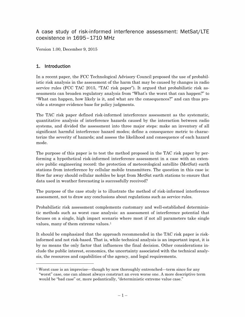
Figure 3. Polar Orbital Exploration Satellite (POES) system elements. (a) 13 meter '2/B' antenna in Fairbanks, AK.14 (b) Example of a near-polar orbit.15

Since the received signal is very weak, a satellite is tracked by a high gain dish antenna such as that shown in Figure 3 (a). The aggregate of all the signals transmitted by cellu-lar mobiles close to the receiver can cause interference. In order to prevent interference, transmissions close to the satellite receiver have to be prevented while data is being re-ceived.

POES satellites transmit at 1698, 1702.5 and 1707 MHz (NTIA 2010, Table 3-1). The Joint Polar-orbiting Satellite System (JPSS) is slated to begin with the launch of the Su-omi NPP satellite in 2016 and will transmit at 1707 MHz (CSMAC 2013, NOAA slide 16, p. 58).

There is currently no GOES operation in the 1695–1710 MHz or adjacent band; it is slated to begin in the 1680-1695 MHz band in 2016 (CSMAC 2013, NOAA slide 16, p. 58). Since the WG-1 Report found that GOES protection radii are considerably smaller than those required for POES (CSMAC 2013, Appendix 7, Table 1 ff.), protection dis-tances are determined by POES operation except for sites where there are only GOES earth stations. This study will therefore limit its attention to POES.

roughly the same time every day. In general, the AM spacecraft orbit in a descending node (crossing from north to south) while the PM spacecraft orbit in an ascending node; see https://directory.eoportal.org/web/eoportal/satellite-missions/n/noaa-poes-series-5th-generation.

14 Source: http://wireless.fcc.gov/services/aws/data/AWS3bandplan.pdf. 15 Source:

http://tornado.sfsu.edu/geosciences/classes/m407_707/Monteverdi/Satellite/PolarOrbiter/Polar_Orbits.html.

(a) (b)

– 7 –

Figure 4. Polar orbit ground track for 24 hours.

The potentially interfering systems we will consider are LTE cellular mobile transmit-ters (LTE “User Equipment,” or “UEs”). We assume that this service is deployed as sep-arate 5 MHz and 10 MHz license blocks, as shown in Figure 1. We will focus our analysis on interference in the upper 1700–1710 MHz B2 block which overlaps with the 1702.5 and 1707 MHz POES reception frequencies.

3. First element: Make an inventory of hazards

The first step in probabilistic risk assessment is to make an inventory of all expected hazards, that is, phenomena that could but won’t necessarily cause harm. Once that is done, we will review the determinants of interference hazards. We do not analyze non-interference hazards such as MetSat system malfunctions and signal strength variabil-ity.

A. Hazards

The hazards to weather satellite (MetSat) operation in 1695–1710 MHz are summarized in Table 1. Observe that there are hazards not due to interference. One can divide inter-ference sources into those transmitting in the same channel as the affected system, and those transmitting in adjacent channels or bands. Mobile cellular services are already present in the adjacent AWS-1 band, and have also been allocated to the co-channel AWS-3 blocks A1 and B1 where MetSat earth stations will continue to operate; see Fig-ure 1.

Note that we only model interference from known, intentional radiators. We leave aside interference due to intermodulation products and spurious emissions, and ignore the risk of intentional jamming.

Source: NOAA (2009), Figure III-4

– 8 –

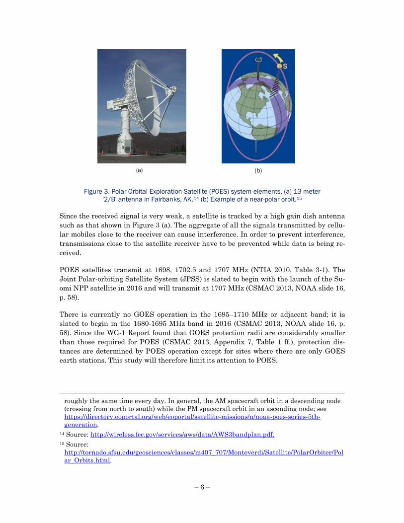
Table 1. Examples of performance hazards to MetSat reception

Persistent

(long-term)† Intermittent (short-term)†

Non-interference hazards

System failure, satellite or receiver failure, operator error, power outage Signal strength loss e.g.due to ionospheric scintillation

Power supply spikes

Co-channel interferers

Persistent weak interference from co-channel operators combined with occasional fading of the satellite signal*

Short-term, strong interference overwhelms a persistent strong desired signal

Out-of-band interference (OOBE) into co-channel

Spill-over from transmissions by AWS-1 mobiles not fully excluded from MetSat channel due to limited AWS-1 adjacent channel filtering

Frequency-adjacent interferers

Adjacent Band Interference (ABI)

Power in AWS-1 band not fully excluded by MetSat adjacent channel selectivity

Intermodulation and spurious emissions

Interference in MetSat channel due to intermodulation of transmissions in adjacent bands

Interference spikes due to spurious emissions

† Long- and short-term interference is defined in SA.1026-4. * Only hazard considered by Fast Track Report and CSMAC WG-1 Report.

i. Non-interference hazards

Radio interference is not the only hazard to the reception of satellite signals. We will consider two categories here: faults and failures, and degradation of the desired signal strength. Since we have not been able to obtain data on the incidence or severity of these hazards, they are not included in the numerical analysis.

Faults and failures include system and device failures (terrestrial or in orbit), device misconfiguration and degradation, physical phenomena, power outages, and operator error. Physical phenomena include mounting stresses (e.g. bending and twisting), elec-trical static, shock, vibration, temperature and humidity extremes, condensation, liq-uids, salt spray, conductive dusts, mold growth, oxidation, corrosion, abrasion, and so on.

The desired satellite signal may be degraded by attenuation between the satellite and the earth station, e.g. through ionospheric scintillation, a rapid fluctuation of radio-frequency signal phase and/or amplitude generated as a signal passes through the iono-sphere.16 The amplitude scintillation index S4 is a commonly used metric for amplitude effects; see Figure 5.

16 The description of scintillation is based on material at

http://www.sws.bom.gov.au/Satellite/6/3,

– 9 –

Figure 5. S4 Scintillation index at GPS L1 (1575.42MHz) observed at the same local time (2300) at all longitudes. Strong scintillation is generally considered to occur when S4 is greater than ~0.6; weak scintillation ranges from 0.3 to 0.6.17

Ionospheric scintillation is a well-known phenomenon that has been studied extensively, in part because it also affects GPS signals.18 It is primarily an equatorial and high-latitude ionospheric phenomenon, although it can occur at lower intensity at all lati-tudes (Figure 5). We suspect it is unlikely to play a role in MetSat reception except in Guam, Hawaii and perhaps Alaska.

ii. Co-channel interference

The canonical analysis of interference to MetSat systems, Recommendation ITU-R SA.1026-4, only considers co-channel interference. SA.1026-4 provides criteria for long-

http://roma2.rm.ingv.it/en/themes/11/ionospheric_scintillation, and http://www.insidegnss.com/node/1579.

17 Source: http://www.sws.bom.gov.au/Satellite/6/3. 18 Conveniently, the commonly used GPS L1 frequency (1575.42 MHz) is quite close to the

band of interest in this study.

– 10 –

and short-term interference protection, defined as interfering signal power in the refer-ence bandwidth to be exceeded no more than 20% and 0.0125% of the time, respectively.

The rationale for the long- and short-term interference cases is discussed in a contribu-tion by the United States to ITU-R Working Party 7B that describes the two circum-stances under which communications performance are degraded (USA Delegation, 2007):

1. Interference levels are present for a large percentage of time so that when the level of communications link signal drops below some minimum level, for ex-ample because of signal attenuation due to ionospheric scintillation, the link margin falls below zero.19

2. Interference levels are high for short periods of time and cause the margin to fall below zero though the communications link is nominally strong.

The time percentages refer to those short time periods when the link performance is de-graded below the performance criterion, which is specified in SA.1025-3 for this service as a bit error rate of 10-6 to be met 99.9% of the time (or equivalently, not exceeded for more than 0.01% of the time).20 The long-term power level for both the communications carrier and the interfering signal refers to a nominal level that may be exceeded no more than 20% of the time. USA Delegation (2007) provides a derivation for the 0.0125% short-term percentage.

In other words, over the long term—defined as up to 20% of the time—fading of the sat-ellite signal combines with relatively low interference levels to cause outage, while short-term bursts of higher interference—required to occur no more than 0.0125% of the time—can occasionally combine with nominal satellite signals to cause outage.

SA.1026-4 uses different elevation angles to calculate the long- and short-term criteria; for the service at issue in this study, 5° and 13° respectively. The long-term interference levels are lower (i.e. more stringent) than the short-term levels. We model both in Sec-tion 5.B.

19 For more on scintillation, see e.g.

http://roma2.rm.ingv.it/en/themes/11/ionospheric_scintillation and http://www.ips.gov.au/Satellite/6/3.

20 The length of these “short time periods” is not specified in SA.1026-4. When discussing the difference between long-term and short-term interference, even the otherwise informative US contribution to the revision to SA. 1026-3 merely states: “There are no long-term inter-ference events. All the interference is limited to some short period of time” (USA Delega-tion, 2007). One assumes these are time scales of the order of seconds, not minutes or hours, given that Note 2 in SA.1026-4 states that “the [critical] time required for initial signal acquisition and synchronization may constitute up to several tens of seconds.”

– 11 –

iii. Interference from transmitters in adjacent bands

Neither SA.1206 nor the Fast Track or WG-1 reports address adjacent band interfer-ence. We assume that the long- and short-term interference protection scenarios defined for the co-channel transmissions also apply in this case.

There is no exclusion zone for AWS-1 services: an interfering mobile can be right next to an earth station receiver. The most likely current source of intentionally radiated harm-ful interference is therefore cellular mobiles transmitting in the adjacent AWS-1 band.

The closest cellular mobiles in frequency are in the AWS-1 A block, 1710–1720 MHz. The three POES center frequencies are 1698, 1702.5 and 1707 MHz.

There are two main ways an AWS-1 mobile could interfere with a MetSat receiver: a small part of its power will be radiated or “leaked” in the adjacent MetSat band, known as out-of-band emission or OOBE; or imperfect filtering in the MetSat receiver admits some of the energy radiated within the AWS-1 band, known as adjacent band interfer-ence or ABI. We model both mechanisms in Section 5.C, for both the long- and short-term interference protection criteria.

B. Determinants of interference

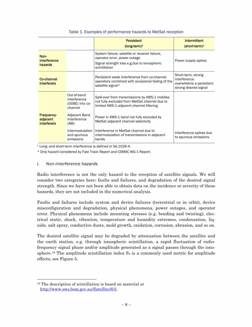
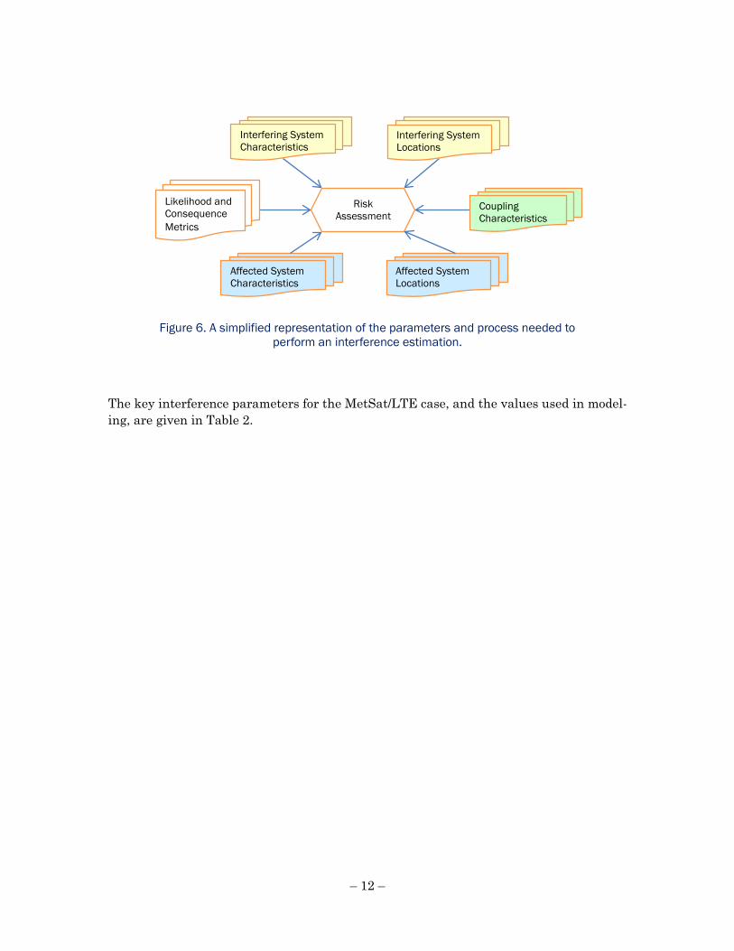
The interaction between two radio systems is affected, among other things, by the loca-tions of the interfering and affected systems, the characteristics of the transmitters and receivers of the two systems, and the coupling between them due to factors such as an-tenna gain patterns and propagation loss. These factors are summarized in Figure 6, which is based on TSB-84A (TR46, 2001, Section 4).21

There are many interference hazards including OOBE and ABI due to frequency adja-cent transmitters, and a variety of co-channel interference hazards ranging from unin-tentional radiators to maliciously operated jammers. Interference may have a single source, or may be the aggregate of a large number of transmitters.

21 IEEE standard 1900.2 offers an alternative categorization, collecting parameters into

groups of frequency-, power-, time-, spatial-, system management-, network- and policy management-related variables (IEEE 2008, section 8, Table 4).

– 12 –

Figure 6. A simplified representation of the parameters and process needed to

perform an interference estimation.

The key interference parameters for the MetSat/LTE case, and the values used in model-ing, are given in Table 2.

Affected System Characteristics

Interfering System Characteristics

Affected System Locations

Interfering System Locations

Coupling Characteristics

Likelihood and Consequence Metrics

Risk Assessment

– 13 –

Table 2. Interference parameter values used in modeling

Parameter Value(s) Characteristics in this study Areas for improvement

Transmitter characteristics

LTE uplink total EIRP per device

CDF for suburban and rural EIRP; values range from 20 dBm to -30 dBm (WG-1 Report, Appendix 3; see Figure 7)

Distribution Use distributions of system loading and traffic buffers to calculate CDF

Channel width Nominal 10 MHz channel; only 9 MHz used, per 3GPP Fixed, single Study effects of 5 and

15 MHz channels

LTE uplink instantaneous channel loading

Fixed, 100%, using assumption in WG-1 Report Fixed, worst case

Use distributions for system loading and traffic model

LTE cellular deployment Following WG-1 Report, Appendix 7, assume hexagonal cell sites with different Inter-Site Distance (ISD) for suburban (1.732 km) and rural (7 km) deployment. This leads to eNodeB densities of 0.386 eNB/km2 (suburban) and 0.024 eNB/km2 (rural); circular suburban/rural boundary at 30 km from MetSat receiver

Fixed, site general

Place base stations following actual population density in site-specific model

LTE mobile location, density

Randomly distributed based on eNodeB densities. 18 UE per base station for 10 MHz channel (WG-1 Report, Appendix 3) imply 1.16 UE/km2 (suburban) and 0.071 eNB/km2 (rural). For co-channel, sample 3 of the 18 (i.e. one per 10 MHz sector)

Random location Fixed density

Use distribution for number of UEs per base station

LTE mobile antenna height

1.5 m for all cases Fixed, typical

LTE mobile antenna gain 0 dBi (values in the field typically order -4 to -8 dBi) Fixed, worst case

Use distribution of antenna gains reflecting fielded devices

Mobile unwanted emissions

ACLR uniformly distributed from 30-40 dB to model actual device performance

Distribution

Receiver characteristics

Satellite orbit and service

POES, HRPT service Fixed Add other POES services; model GOES receivers

Center Frequency (MHz) 1707 MHz; nearest AWS-1 band (POES also transmits at 1698 and 1702.5 MHz)

Fixed, extreme case

Model interference to all three frequencies

Receiver center frequency, 3 dB bandwidth, noise figure

1.33 MHz (representative value, based on Fast Track Report, Appendix A)

Fixed, representative

Frequency dependent rejection (dB)

On-tune rejection 0.5 dB = 10log(1.5 MHz/1.33 MHz); off-frequency rejection not computed

Fixed

– 14 –

Receiver selectivity (relative attenuation as a function of frequency offset)

-3 dB @ +/- 0.665 MHz -20 dB @ +/- 1.34 MHz -60 dB @ +/- 12.0 MHz (least selective receiver, Fast Track Report, Appendix A, Table A-5)

Fixed, extreme case

Receiver system noise temperature

5° elevation : 320 K 13° elevation : 210 K (Table 2, SA.1026-4 for HRPT)

Fixed, conservative

Main beam antenna gain of receiver (dBi)

43.1 dBi (largest value reported in Fast Track Report, Appendix A)

Fixed

Antenna model Azimuth and elevation gain relative to main beam direction, using ITU-R F.1245

Fixed, conservative

Elevation angle Per Table 2, SA.1026-4 for HRPT: Long-term protection: 5° Short-term protection: 13°

Fixed, extreme case

Antenna height above local terrain

21 m (representative value, based on Fast Track Report, Appendix A)

Fixed, representative

Azimuth Not specified since using an area-general model N/A

Transmitter-Receiver Coupling

Propagation loss (dB) Area general model: 1 km and beyond: Extended Hata (Drocella et al. 2015) 20 m to 1 km: interpolation between free space at 20 m and Extended Hata at 1 km

Distribution Implement ITM Area Mode model as comparison; use site-specific model

Location variability 1 km and beyond: log-normal distribution, zero mean, 8 dB standard deviation For 20 m to 1 km, interpolate between 0 dB and 8 dB standard deviation.

Distribution

Body loss at UE; clutter loss

0 dB Fixed, worst case

Use distributions for body loss

Additional losses (dB) Receiver insertion loss, cable loss, polarization mismatch loss, etc. Fixed, 1 dB (following WG-1 Report, Appendix 7)

Fixed

i. Transmitter characteristics

The amount of power transmitted by an interfering cellular mobile is a key consideration in the amount of interference experienced by a receiver.

We use the cumulative distribution function (“CDF”) of UE Equivalent Isotropic Radiat-ed Power (“EIRP”) published in the WG-1 Report; see Figure 7. The transmit power var-ies, with median values of -13 dBm and -3 dBm for the suburban and rural cases, respec-tively, and a maximum of +20 dBm.

– 15 –

This distribution was calculated on the assumption that every base station is fully load-ed, and that all mobiles have their buffers full at all times (CSMAC 2013, Appendix 3, pp. 3-2 and 3-4). This is a rather conservative assumption.22 Since the critical time win-dow for POES operation is only a few tens of seconds, however, the assumption of full loading, although worst case, seems a reasonable default in the absence of data from cel-lular operators on the statistics of cell loading.23

Figure 7. Cumulative distribution function of transmitted power per scheduled

mobile.

Another important consideration is the location of transmitters. We follow the WG-1 Re-port in assuming a homogenous, isotropic hexagonal cell structure with 18 mobiles per 10 MHz channel associated with each base station.24 This is evidently not a real-world

22 The average base station load in a cellular system is 60% or so; busy sites will see peak

loading that that occupies the whole channel. Even at less than full loading one will occa-sionally see all uplink resources used for statistical reasons. However, since LTE is a mo-bile system, “fully loaded” doesn’t map to 100% utilization of physical resource blocks (PRBs, a small block of time and frequency) since a percentage of PRBs within a sector are reserved for handover.

23 Recommendation ITU-R SA.1026-4, Note 2 explains that “the time required for initial sig-nal acquisition and synchronization may constitute up to several tens of seconds out of total satellite visibility periods averaging on the order of nine minutes.”

24 We assume three 120° sectors per base station, with each sector using the same 10 MHz. Each sector serves six UEs per 10 MHz, each using a 1.5 MHz channel. This results in 18 concurrently active UEs per base station.

Source: CSMAC (2013), Appendix 3-3

– 16 –

deployment pattern, but is appropriate for a generic, non-site-specific analysis such as this.

ii. Receiver characteristics

In general, the characteristics of individual receivers deployed in a given service can vary, and their locations may be unknown—for example, in TV reception. Matters are greatly simplified in this case because the affected MetSat receivers are a small, well-defined population with known characteristics and locations (Fast Track Report, Appen-dix A).

For the purposes of this exercise we will assume a receiver with the highest earth sta-tion antenna gain (43.1 dBi) and the weakest adjacent channel selectivity (-60 dB at +/- 12.0 MHz) from among those listed. POES satellites provide a number of different data feeds.25 We will model the High Resolution Picture Transmission (HRPT) service since it is the highest bandwidth service, and thus most susceptible to interference.26 We use the receiver system noise temperature specified for the HRPT service in SA.1026-4, Table 2, and the antenna model given in ITU-R F.1245-2 (ITU-R 2012).

Since the 1.5 MHz LTE UE channel is wider than the 1.33 MHz MetSat receiver chan-nel, not all the power transmitted by the UE that overlaps the MetSat channel is admit-ted to the receiver. The reduction in power is quantified by the on-tune rejection (OTR), defined as:

𝑂𝑂𝑂𝑂𝑂𝑂 = 𝑚𝑚𝑚𝑚𝑚𝑚 �0, 10𝑙𝑙𝑙𝑙𝑙𝑙 �𝐵𝐵𝑡𝑡𝑡𝑡𝐵𝐵𝑟𝑟𝑡𝑡

�� = 0.5 𝑑𝑑𝐵𝐵 (1)

where

𝐵𝐵𝑡𝑡𝑡𝑡 emission bandwidth of the transmitter = 1.5 MHz 𝐵𝐵𝑟𝑟𝑡𝑡 3 dB selectivity of the receiver = 1.33 MHz

Following the WG-1 report, we subtract 1 dB for additional losses associated with MetSat receiver insertion loss, cable loss, polarization mismatch loss, etc.

iii. Transmitter-Receiver Coupling

The two main factors influencing the coupling between interfering transmitters and af-fected receivers are the attenuation of transmitted energy along the paths between them (termed path loss), and the effects of antennas at the two endpoints.

25 See https://eosweb.larc.nasa.gov/ACEDOCS/data/appen.c.1.html. 26 The imagery is derived from the Advanced Very High Resolution Radiometer (AVHRR),

and the term AVHRR is sometimes used to refer to HRPT service.

– 17 –

We use the Extended Hata propagation model defined in Drocella et al. (2015, Section 4.7 and Appendix A) to calculate median path loss between individual UEs and the MetSat receiver.

Uncertainty about the path loss between transmitters and the receiver leads to uncer-tainty in the amount of interfering power. There are broadly speaking two kinds of prop-agation uncertainty: differences in path loss as the transmitter moves about in time, po-sition or frequency in a limited region, sometimes called fading and referred to in this document as location variability; and differences between model predictions for attenua-tion over larger distances.

Location variability is often modeled by adding a zero mean random variable to the me-dian path loss; we use a log-normal variable with 8 dB standard deviation (cf. Table A-1 in Drocella et al. (2015), summarizing the Okamura et al. measurements). We ignore temporal fading. We also ignore body loss, i.e. attenuation of the UE signal due to atten-uation through the user’s body.

Differences between propagation models lead to systematic differences between simula-tions performed using different models. Two leading propagation models classes are Ir-regular Terrain Models that are optimized for longer-range propagation from high transmitters, take terrain into account, but ignore clutter; and the Okumura-Hata fami-ly of models that are optimized for shorter-range propagation, ignore terrain, and take clutter into account. We have elected to use an Extended Hata model since this is com-monly used in cellular deployment studies and accounts reasonably well for the subur-ban clutter that we expect around a MetSat receiver.

Turning to antenna effects, cellular mobiles are assumed to be radiating uniformly in all directions. We assume 0 dBi UE antenna gain.

In contrast, MetSat earth station antennas are highly directional, with the 30–40 dBi maximum gain along the main beam direction. The antennas follow satellites across the sky as they appear over the horizon, rise towards the meridian, and then set. The amount of interference admitted to the receiver depends on the gain of the antenna in the direction of a particular UE. Since the interfering transmitters are at ground level, the maximum coupling (and thus maximum interference) will occur when the earth sta-tion antenna is at its lowest elevation above the horizon. We follow SA.1026-4 and the WG-1 Report in assuming a minimum elevation of 5°.

4. Second element: Define a consequence metric

A consequence metric quantifies the severity of an interference hazard. Since the goal of risk analysis is to treat all hazards under the same rubric, there should be a small num-ber of consequence metrics (ideally just one) that characterize the severity of hazards in a uniform way.

– 18 –

However, there are in practice many potential consequence metrics. One can distinguish three broad categories:

• Corporate metrics: Examples include impact on the ability to complete a mission (particularly for government entities); and increased capital expenditure, loss in revenue or loss of profit (particularly relevant to the private sector).

• Service metrics: These measure the quality of the specific service that the radio link supports. Two broad sub-categories are:

o Availability (time period or time percentage of outage; number or per-centage of receivers without service; etc.)

o Quality (bit error rates for data services, range reduction for radar sys-tems, acquisition time and location accuracy for navigation services, Mean Opinion Scores for broadcasting, etc.)

• RF metrics: Quantities observable in the radio frequency (thus “RF”) environ-ment, such as changes in interference-to-noise ratio (I/N), signal to interference and/or noise ratios (SINR, C/I), absolute interfering signal level, receiver noise floor degradation, and so on.

We will now examine various candidate consequence metrics for the MetSat service.

A. Corporate metrics

The NOAA Office of Satellite and Product Operations maintains a web site reporting operational status for each GOES and POES satellite.27 Color status indicators (green, yellow, red) are given for the subsystems on every space platform, but numerical metrics are not given. We have not found data on the operational status or service level of earth stations. We have also been unable to obtain information on the performance indicators that system managers such as NOAA use to measure the performance level of weather satellites.

Thus, to the best of our knowledge, there are no publicly available corporate metrics of the ability of a MetSat service to complete the forecasting mission, even at the relatively granular level of image quality.

We note some anecdotal evidence, however. A sampling of images archived by the Ju-neau, AK station of the National Weather Service collected over a few days in July 2015 suggests that of the order of 10 percent of images received at this site show significant degradation, i.e. noticeable contiguous regions of lost scan lines; some examples are shown in Figure 8.

27 http://www.ospo.noaa.gov/Operations/GOES/status.html,

http://www.ospo.noaa.gov/Operations/POES/status.html.

– 19 –

These images illustrate the importance of obtaining baseline hazard information: the risk of RF interference needs to be assessed in the context of the seemingly severe image degradation that already occurs—at least at one site—in the absence of interference from new services sharing the band. (For further discussion of baseline performance, see Section 7.i.)

Figure 8. Archived HRPT images from National Weather Service, Juneau, AK.28

B. Service metrics

Table 2 of SA.1026-4 (the international reference for MetSat coexistence analysis) lists three factors that could be used as consequence metrics:

1. The percentage of time that the link margin is not met

2. Bit-error ratios (link bit-error ratio, data handling error ratio, and overall re-ceived bit-error ratio)

3. The fraction of interference-free margin consumed by interference (called q)

The first two are service metrics under our definition, and address availability and qual-ity, respectively.

Unfortunately, we have been unable to find ITU-R documentation on how these parame-ters are defined, how they are related to other tabulated parameters, or the relationship between these metrics and image quality.29

28 Source: http://pajk.arh.noaa.gov/satellite/poes.php

– 20 –

The percentage of time that the link margin is not met appears to determine the SA.1026-4 interference protection criterion, which is a power level not to be exceeded for more than a specified percentage of time. The percentage of link outage is an attractive consequence metric in principle, since it affects received image quality. However, it is not usable in practice without a formula for the link between the interference power and percentage of link outage. We have not found any documentation of the formulas and key parameters (such as the distribution of received power) that were used to derive the values in SA.1026-4.

The bit-error rate (“BER”) target in SA.1026-4 appears to have been taken from SA.1025-3, and is used as a minimum performance level. SA.1026-4 implies that its in-terference power values ensure that the SA.1025-3 criterion—that a minimum bit-error ratio of 10-6 is ensured at least 99.9% of the time—is met under all circumstances.

Since BER is a function of Eb/N0, the ratio of energy per bit to noise power spectral den-sity, it could be computed given the distribution of Eb/(N0+I0) values, where I0 is the in-terference power spectral density. For example, BER = 0.5 erfc(sqrt(Eb/N0)) for polar NRZ, BPSK and QPSK modulations. However, we have been unable to identify a func-tional form for the relationship between BER and Eb/N0 in SA.1026-4 or any related documentation. We have also not been able to determine the probability distribution of Eb assumed in SA.1026-4.

C. RF metrics

The margin consumed by interference given in SA.1026-4 is an RF metric. It is de-fined in SA.1022-1 (ITU-R 1999) in formulas for the permissible interference:

𝐼𝐼0 = 𝑁𝑁0(𝑀𝑀𝑞𝑞 − 1) 𝑓𝑓𝑙𝑙𝑓𝑓 𝑀𝑀 > 𝑀𝑀𝑚𝑚𝑚𝑚𝑚𝑚

𝐼𝐼0 = 𝑁𝑁0�𝑀𝑀𝑚𝑚𝑚𝑚𝑚𝑚𝑞𝑞 − 1� 𝑓𝑓𝑙𝑙𝑓𝑓 𝑀𝑀 ≤ 𝑀𝑀𝑚𝑚𝑚𝑚𝑚𝑚

(2)

(3)

where

I0 interference spectral density at the affected receiver (watt) N0 noise density ratio at the affected receiver (watt) M interference-free margin for the receiving system (ratio) q the fraction of the interference-free margin M expressed in dB that inter-

ference is allowed to consume30 Mmin the smallest interference-free margin for which the affected system must

be fully protected (ratio)31 29 We were not able to obtain assistance from staff who drafted key US contributions to this

standard due to NOAA workload requirements and non-availability of subject matter ex-perts.

30 The q values given (without explanation) in SA.1026-4 are 0.33 or 0.6 for long-term protec-tion and 1.0 for short-term protection.

– 21 –

Note that one can calculate an interference-to-noise ratio I/N from these equations, alt-hough SA.1026-4 does not do so. It will be influenced by the desired signal strength due to the dependence on the margin M; both increased antenna gain or a greater antenna elevation above the horizon will improve the margin and thus I/N.

Inverting these formulas allows one to express the margin consumed q as a function of M and N0, and a calculation of I0:

𝑞𝑞 = 10𝑙𝑙𝑙𝑙𝑙𝑙 �1 + 𝐼𝐼0

𝑁𝑁0�

𝑀𝑀𝑑𝑑𝑑𝑑 (4)

where

𝑀𝑀𝑑𝑑𝑑𝑑 log-scale interference-free margin for the receiving system (dB)

One could thus use the results of Monte Carlo simulation to plot the likelihood of q ex-ceeding a certain value. Since the amount of margin consumed by interference is a key concern for satellite communication engineers, a cumulative distribution function of q is therefore an attractive consequence metric.

A second candidate RF consequence metric, and the one that we will use in this study, is the interfering signal power. SA.1026-4 specifies interfering signal power levels not to be exceeded more than 20% and 0.0125% of the time, defined as the long- and short-term protection criteria, respectively (ITU-R 2009, Table 1). (This is discussed in more detail in Section 5.A.)

The key parameter studied in the Fast Track and WG-1 reports was the protection distance at which the interference protection criterion at a specific earth station is met. The protection distance is the radius of a circle around the earth station within which co-channel mobiles are not allowed to transmit without permission of the MetSat operator. We use the interfering signal power that meets the SA.1026-4 criteria to derive an ex-clusion distance within which LTE mobiles would not be allowed to operate.

Since a judgment about the desirability of a new service requires assessing the risk of harmful interference to incumbent services, and since harmful interference is defined for regulatory purposes as a service metric of sorts, corporate or service metrics are in prin-ciple preferable to RF metrics.32 However, in most cases we are aware of—such as televi-

31 The value for Mmin for all systems listed in SA.1026 is given there (without explanation) as

1.318 = 1.2 dB. 32 Harmful interference is defined in Article One of the ITU Radio Regulations, and incorpo-

rated into national regulations such as 47 C.F.R. 2.1 in the U.S., as “Interference which en-dangers the functioning of a radionavigation service or of other safety services or seriously degrades, obstructs, or repeatedly interrupts a radiocommunication service operating in ac-cordance with these Regulations.”

– 22 –

sion broadcasting, mobile public safety, and cellular service—the mapping of RF metrics to service degradation is ambiguous at best; an exception is the effect of RF interference on radar target detection (Sanders et al., 2006). Our analysis will thus focus on RF met-rics since they are more readily available and easier to model, even though their connec-tion to service or corporate metrics is often tenuous.

In summary, we will characterize interference risk as the combination of an RF metric—specifically, the aggregate interfering signal power—and its likelihood for different haz-ards such as co-channel and adjacent band transmitters.

5. Third element: Assess likelihood and consequence

The next element of the analysis is estimating the likelihood and consequence of each of these hazards, given the operational parameters that affect interference (see Table 2 on p. 13), deployment constraints and operating rules.

Quantifying likelihood is relatively straightforward: we take it to be the probability of occurrence of a hazard. However, the result depends on the population that is sampled. An appropriate population for regulatory decisions is likely to be all relevant transmit-ters and receivers in the region at issue, in this case a license area around a MetSat re-ceiver site.

We use probability distributions for interference parameters wherever possible (such as the distribution of cellular mobile transmit power in Figure 7), and combine them with fixed-value parameters to yield a probability distribution for the consequence metric.

The result will be quantitative versions of the qualitative likelihood-consequence chart shown in Figure 2 on p. 4.

A. Modeling method

Our modeling approach builds on the method used by NTIA staff to calculate exclusion and protection zones in the Fast Track and WG-1 reports, respectively.

We perform an electromagnetic compatibility analysis between cellular mobile transmit-ters (UEs) and earth station receivers for Polar Operational Environmental Satellites (POES) transmitting in the 1695–1710 MHz band. We model interference with POES transmissions at 1707 MHz. We assume the service is High Resolution Picture Trans-mission (HRPT) imagery since it is the most susceptible to interference.

We model a generic POES receiver by reference to receiver performance parameters in the Fast Track Report (NTIA 2010, Appendix A). The parameter values we use are doc-umented in Table 2.

In modeling the characteristics of UEs, we follow the assumptions of Appendix 3 of the WG-1 Report:

– 23 –

• We use a UE density calculated by assuming base stations arranged in uniform hexagonal cells with inter-site distances of 1.732 and 7 km for suburban and ru-ral deployments; this results in a base station density of 0.385 and 0.024 per sq. km for suburban and rural areas, respectively.

• UEs are randomly distributed at an average of 18 per cell, leading to a density of 6.9 and 0.42 UEs per sq. km for suburban and rural areas, respectively.33 In the co-channel case we sample 3 UEs per cell (see Section 5.B for discussion).

• The MetSat receiver is surrounded by suburban cells out to a 30 km radius, and rural cells beyond that.

We sample the transmit power of each UE separately, anew for each Monte Carlo itera-tion, from the cumulative distribution functions for EIRP calculated by WG-1 (see Figure 7); we thus adopt the protective assumptions about 100% system loading, full buffer traf-fic, etc. given in the WG-1 Report (CSMAC 2013, Appendix 3-3, 3-4).

Table 3. Extended Hata model: Key parameter values

Parameter Value

Frequency 1707 MHz

Height of mobile device 1.5 m

Height of base (earth) station 21 m

Minimum, maximum† distances 1 km, 100 km

Breakpoint distance* 16.2 km

† We do not model out to the maximum distance. * The breakpoint distance is a parameter in Drocella et al. (2015) due to its “two-slope” approach.

We model propagation losses using the extended Hata model developed by the NTIA for 3.5 GHz exclusion zone analysis (Drocella et al. 2015, Section 4.7 and Appendix A). A suburban correction factor was applied to the propagation model in calculating the prop-agation loss for all UEs (see Drocella et. 2015, Equation A-14). This model provides a median attenuation as a function of distance between the transmitter and receiver; key model parameter values are given in Table 3. For each UE-MetSat link we add a location variability sampled from a zero mean, log-normal distribution with 8 dB standard devia-tion, as discussed in Section 3.B.iii above.

The interference power levels at the federal MetSat receiver are calculated by aggregat-ing the delivered signal strength from all LTE mobiles between a variable inner radius—the exclusion distance—and a fixed maximum radius. The maximum distance is chosen

33 We assume 10 MHz co-band and adjacent band LTE operation, with six 1.5 MHz UE chan-

nels per 10 MHz band (UE transmissions thus occupy 9 MHz; there are 0.5 MHz guard band at the lower and upper ends of the bands). Each cell has three sectors, for a total of 18 UEs per band per cell.

– 24 –

to be far enough beyond the exclusion distance that it includes all UEs that will make a contribution to the aggregate interference. The contribution of UEs drops off with dis-tance; in practice we find that increasing the maximum radius more than about 10 km beyond the exclusion distance makes no difference to the received interference.

Since the UEs are deployed uniformly around the earth station location and we use an area propagation model, there is no dependence on the earth station antenna pointing direction (i.e. azimuth) in this study.

Since a number of parameters take a range of values, we use Monte Carlo modeling.34 In short, our algorithm is as follows:

For each successive inner radius, do the following for N iterations (see Table 5 for itera-tion counts):

• Place UEs randomly between the inner radius and the maximum simulation ra-dius, using suburban or rural density depending on location

• For each UE: o calculate distance to the receiver o calculate median path loss as a function of distance o add location variability sampled from distribution, and subtract OTR and

additional losses o subtract ACLR sampled from distribution, or ACS for adjacent band cases o sample EIRP from the distribution o calculate gain given calculated angle between antenna boresight direction

and vector to UE o calculate net interfering power for each UE from the above, using equa-

tions (5) to (10) • Sum interfering power from all UEs

The probability distributions we use are listed in Table 4.

Table 4. Probability distributions used in Monte Carlo modeling

Variable Properties

UE transmit power Distributions for suburban and rural UEs (CSMAC 2013, Appendix 3-3), see Figure 7

UE location Randomly sampled in the plane with suburban or rural density per Table 2 above

Location variability in path loss

• Beyond 1 km: zero mean log-normal distribution with 8 dB standard deviation • Less than 1 km: zero mean log-normal distribution with standard deviation

interpolated as a function of log distance between 0 dB at 20 m and 8 dB at 1 km

ACLR Uniform distribution between 30 and 40 dB

34 The MATLAB code implementing the Monte Carlo model was developed by Uri Livnat of

the FCC Technical Analysis Branch, and is given in the Appendix.

– 25 –

Salient modeling parameter values are listed in Table 5. We calculate a large number of possible values for the aggregate interference power for each value of the inner radius, for each of the hazards studies; this number is listed in the “# iterations per radius” col-umn of Table 5.

Table 5. Monte Carlo modelling scenarios

Channel Interference time scale

Elevation angle

Min radius

Max radius

Inner radii for which interference calculated

# iterations per radius

Co-channel long term 5° 1 km 70 km 1km, out to 50 km 10,000

Co-channel short term 13° 1 km 70 km 1km, out to 4 km 1,000,000

Adj channel, OOBE long term 5° 20 m 20 km* Single inner radius: 20m 100,000

Adj channel, ABI long term 5° 20 m 20 km* Single inner radius: 20m 100,000

Adj channel, OOBE short term 13° 20 m 20 km* Single inner radius: 20m 1,000,000

Adj channel, ABI short term 13° 20 m 20 km* Single inner radius: 20m 1,000,000

* The contribution of interference beyond 20 km is negligible in cases with an inner radius 4 km or less; in fact, we find that extending the max radius beyond 10 km does not change the results.

In order to calculate an exclusion radius, we use an interference protection criterion (IPC) calculated following the method in SA.1026-4 that assumes two interference sce-narios:

• Long-term interference: interfering signal power in the receiver reference bandwidth to be exceeded no more than 20% of the time. This scenario corre-sponds to a 5° antenna elevation in SA.1026-4, Table 2.

• Short-term interference: interfering signal power in the receiver reference bandwidth to be exceeded no more than 0.0125% of the time. This scenario corre-sponds to a 13° antenna elevation in SA.1026-4, Table 2.

The IPC for these scenarios are given in Table 6; we analyze both the long- and short-term scenarios below. For a 43.1 dBi antenna and a 1.33 MHz receiver bandwidth, the long-term IPC is -108 dBm, and the short-term IPC is -101 dBm. Figure 9 shows how the received co-channel interference power decreases with increasing inner (i.e. exclusion) radius for the long-term protection scenario.

Table 6 contains two sets of parameter values: (1) the HRPT protection criteria given in SA.1026-4 Table 2, and (2) the criteria corresponding to the receiver parameters we use. Since our model assumes less earth station gain and a narrower receiver bandwidth than the example given in SA.1024-6, our values are lower than the values listed there.

– 26 –

A spreadsheet showing the calculations leading to these values is available on Dropbox via http://bit.ly/1SxrYfW.

We assume that the variation in transmitter location and path loss between successive Monte Carlo iterations reflects the temporal variation of interference power. Thus, we take the stipulation in SA.1026-4 that the IPC should be exceeded no more than 20% of the time to correspond to an exclusion radius chosen at the 20th percentile of the com-plementary cumulative distribution function (“CCDF” or exceedance probability) of ag-gregate interference powers reported below.

Table 6. MetSat interference protection criteria calculated using method in SA.1026-4, Table 2

Service and model Recorded data playback

(HRPT) ITU-R SA.1026-4, Table 2

Recorded data playback (HRPT)

Values used in this study

Protection scenario Long-term Short-term Long-term Short-term

Percentage of time for link margin not met, p 0.05% 20% 0.05% 20%

Elevation angle (exceeded for p) 5° 13° 5° 13°

Earth station antenna gain (dBic) 46.8 43

Receiver reference bandwidth (kHz) 5,334 1,331

Receiver system noise temperature (K) 320 210 320 210

Data rate (dB-Hz) 64.2 64.2

q factor: fraction of margin (in dB) consumed by interference 0.6 1 0.6 1

Power margin M (dB) 9.6 12.7 5.9 6.0

Minimum margin Mmin (dB), used if power margin M is negative 1.2 1.2

I0/N0 (dB) (inferred from SA.1026-4 values using SA.1022-1) 4.4 12.5 1.0 8.4

Percentage of time for interference criterion 20% 0.0125% 20% 0.0125%

Interference protection criterion (dBm) -98 -91 -108 -101

* Input values that affect calculated IPC in bold type; cells where input values differ between the SA.1026-4, Table 2 example and our model are highlighted.

We model interference from transmitters in the adjacent AWS-1 band by assuming only interference from the 10 MHz A block (1710–1720 MHz) adjacent to the MetSat receiver at 1707 MHz. We assume a 20 meter exclusion zone around the MetSat receiver, and model the aggregate interference from a sea of UEs distributed as before from this radi-us outwards. Since the extended Hata model only applies for distances greater than 1

– 27 –

km, we use a linear interpolation between free space path loss at 20 meters and the Hata value at 1 km.35 We likewise interpolate the value of the location variability be-tween 0 dB at 20 m and 8 dB at 1 km.

B. Co-channel transmitter

In the co-channel case we consider LTE operation in the same band as the MetSat re-ceiver. As noted in Section 5.A above, we posit LTE UEs that transmit in 1.5 MHz chan-nels; a particular UE will hop in frequency between the six available 1.5 MHz channels in its 10 MHz block. Since we assume that all UEs are always transmitting, there will always be one UE transmission overlapping with the MetSat receiver bandwidth of 1.33 MHz.36 Thus, we sample the power of three UEs per cell (one per sector, with six chan-nels per sector), i.e. a density of 1.16 and 0.071 UE per sq. km for suburban and rural areas, respectively.

Since not all of the transmitted power in a 1.5 MHz LTE channel is admitted into the 1.33 MHz MetSat receiver, we apply an on-tune rejection (OTR) correction factor of 0.5 dB as calculated in eq. (1) on p. 16.

In each Monte Carlo iteration, UEs are distributed randomly between an inner and out-er radius following the suburban and rural densities defined above.

i. Co-channel interference: long-term protection criterion

The interference power for the kth UE is calculated using the following formula:

𝑃𝑃𝑘𝑘 = 𝑂𝑂𝑘𝑘 − 𝑂𝑂𝑂𝑂𝑂𝑂 − 𝐿𝐿𝑘𝑘 − 𝐿𝐿𝑎𝑎𝑑𝑑𝑑𝑑 − 𝐺𝐺(5°,𝜑𝜑𝑘𝑘) (5)

where

𝑘𝑘 k-th UE; sample 3 UEs per base station out of total of 18 𝑃𝑃𝑘𝑘 interference power at the receiver input from the kth UE (dBm) 𝑂𝑂𝑘𝑘 transmitted power of the kth UE (dBm) 𝑂𝑂𝑂𝑂𝑂𝑂 on-tune rejection of 0.5 dB

35 The interpolation is linear in log(attenuation) against log(distance), that is it follows the

form log(attenuation) = m*log(distance) + c, where m is the slope and c the intercept.36 We assume that the 1.33 MHz MetSat bandwidth falls completely within a 1.5 MHz LTE UE channel. In practice, the MetSat bandwidth may be fall across the boundary between two UE channels, but since we are sampling very large number of UEs a very large number of times, this refinement will make a negligible difference.

36 We assume that the 1.33 MHz MetSat bandwidth falls completely within a 1.5 MHz LTE UE channel. In practice, the MetSat bandwidth may be fall across the boundary between two UE channels, but since we are sampling very large number of UEs a very large number of times, this refinement will make a negligible difference.

– 28 –

𝐿𝐿𝑘𝑘 path loss between the kth UE and the antenna input (dB) 𝐿𝐿𝑎𝑎𝑑𝑑𝑑𝑑 additional losses of 1 dB 𝜑𝜑𝑘𝑘 opening angle between antenna pointing direction and vector to k-th UE 𝐺𝐺(5°,𝜑𝜑𝑘𝑘) earth station antenna gain in the direction of the kth UE, with main

beam at 5° elevation above the horizon (dBi)

The received interference powers of all the UEs are converted to watt, summed, and the result converted to dBm.

We calculate 10,000 aggregate interference power values for each value of the inner ra-dius between 1 and 70 km with the earth station antenna gain set to 5°. Figure 9 shows the aggregate interference from mobiles for successively larger inner radii, i.e. larger exclusion zones.

Figure 9. Chart of co-channel, long-term aggregate interference for successive inner radius values.

Observe that the -108 dBm long-term IPC at the 80th percentile is met even for the smallest, 1 km radius. (We will show in the next sub-section that the binding constraint is the short-term IPC; it is exceeded at 1 km, and a larger exclusion radius will be re-quired to ensure it is met.)

It is clear from Figure 9 that the maximum value fluctuates dramatically. In order to examine the stability of the percentile criteria, Figure 10 shows how the value of some

Long-term IPC for 43.1 dBi antenna gain: -108 dBm

-121 dBm

– 29 –

statistics—the 80th and 99th percentile, and the maximum—change as the number of Monte Carlo iterations for each radius increases.

The value at the 80th percentile (the statistic used to calculate the SA.1026-4 long-term protection criterion, which is the interference power that may not be exceeded more than 20% of the time) is essentially unchanged as the number of iterations increases from 1,000 to 5,000 and 10,000; thus the 80th percentile (the value exceeded no more than 20% of the time) is a reliable statistic for the long-term analysis.

After about 1,000 iterations, the 99th percentile value changes only slightly (by a few dB at most) as the number of iterations grows, since more outliers are generated.

It is clear that the maximum is not a usable statistic since it grows sharply and unpre-dictably with the number of iterations, and varies dramatically from one radius to the next.37 The maximum values at different radii also don’t increase monotonically with the number of iterations; for example, even after 10,000 iterations per radius, the maximum for a 7 km inner radius is less than the maxima for 8 and 9 km.

Checking that the 0.0125% not-exceeded short-term IPC is met will require considerably more iterations than for the 20% case since the fraction of exceedances is so small; we do 1 million iterations to test the short-term criterion.

We now develop the results shown in Figure 9 for eventual presentation in a risk chart. The first step is to convert the data into a distribution of the probability that the long-term IPC of -108 dBm is exceeded for each radius.

37 Since at least one of the distributions in the model (the location variability) is a log-normal

distribution and thus has no maximum value, the value of the maximum interference pow-er will grow arbitrarily large with a large enough number of iterations.

– 30 –

Figure 10. Change in statistics with number of iterations: co-channel, long-term interference scenario.

Consider the 1 km radius in Figure 9, shown again in Figure 11. The Monte Carlo model has calculated 10,000 values for the aggregate interference power at that distance; the lines on the figures identify a few boundaries of the distribution of values. The 80th per-centile value is -112 dBm, as shown in Figure 11; that is, 20% of the Monte Carlo results for a 1 km inner radius yielded an aggregate interference power equal to or greater than -112 dBm.

– 31 –

Figure 11. Chart of long-term aggregate interference from mobiles beyond inner radius, with 80th percentile values marked for 1 km.

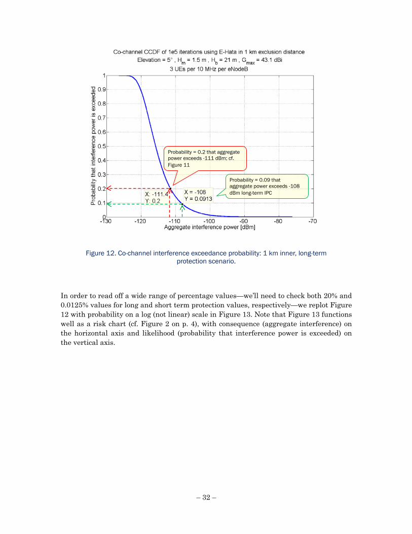
Figure 12 represents the “vertical slice” of the results for just the 1 km inner radius in Figure 11. It shows the exceedance probability (i.e. the complementary cumulative dis-tribution function) of all the results for 1 km, i.e. the value on the vertical axis is the probability that the interference power on the horizontal axis is met or exceeded in the set of Monte Carlo results.

The -112 dBm value is marked, with its corresponding probability of 0.2 (i.e. 20%) that this interference power is met or exceeded. The -108 dBm long-term IPC is met or ex-ceeded only 9% of the time, and this interference protection criterion is therefore met with a 1 km exclusion radius.

(Note that choosing a different time percentage that the 20% specified in SA.1026-4 will yield a different radius. For example, -108 dBm is exceeded no more than 1% of the time—the 99th percentile in Figure 9—with a 4 km exclusion radius. If one uses the max-imum value over 10,000 iterations, in spite of the caveats about using the maximum dis-cussed above, the result is approximately a 10 km radius.)

Figure 9 also allows one to read off exclusion radii for different IPCs; for example, the choice of -121 dBm yields a long-term protection radius, i.e. one where the IPC is not ex-ceeded more than 20% of the time, of 6 km.

20% of runs yield aggregate interference power GREATER than -112 dBm for 1km inner radius

80% of runs yield aggregate interference power LESS than -112 dBm for 1 km

80th percentile at 1 km: -112 dBm

– 32 –

Figure 12. Co-channel interference exceedance probability: 1 km inner, long-term protection scenario.

In order to read off a wide range of percentage values—we’ll need to check both 20% and 0.0125% values for long and short term protection values, respectively—we replot Figure 12 with probability on a log (not linear) scale in Figure 13. Note that Figure 13 functions well as a risk chart (cf. Figure 2 on p. 4), with consequence (aggregate interference) on the horizontal axis and likelihood (probability that interference power is exceeded) on the vertical axis.

Probability = 0.2 that aggregate power exceeds -111 dBm; cf. Figure 11

Probability = 0.09 that aggregate power exceeds -108 dBm long-term IPC

– 33 –

Figure 13. Co-channel interference exceedance probability: 1 km inner radius, long-term protection. Same data as Figure 12, but using a logarithmic scale for

probability.

ii. Co-channel interference: short-term protection criterion

The long-term protection calculation indicates an exclusion radius of less than 1 km. We now check whether the short-term protection criterion is met at this radius.

The interference power for the kth UE is calculated using the following formula:

𝑃𝑃𝑘𝑘 = 𝑂𝑂𝑘𝑘 − 𝑂𝑂𝑂𝑂𝑂𝑂 − 𝐿𝐿𝑘𝑘 − 𝐿𝐿𝑎𝑎𝑑𝑑𝑑𝑑 − 𝐺𝐺(13°,𝜑𝜑𝑘𝑘) (6)

where the variables are as in eq. (5), and

𝐺𝐺(13°,𝜑𝜑𝑘𝑘) earth station antenna gain in the direction of the kth UE, with main beam at 13° elevation above the horizon (dBi)

The received interference powers of all the UEs are converted to watt, summed, and the result converted to dBm. Figure 14 shows the short-term results (13° antenna elevation)

Consequence

Likelihood

Probability = 0.09 (9%) that aggregate power exceeds -108 dBm long-term IPC; up to 20% exceedance allowed

– 34 –

for 1, 2 and 3 km inner radii, corresponding to the long-term result (5° elevation) in Fig-ure 13.

The short-term protection criterion is that an aggregate interference power of -101 dBm should be exceeded no more than 0.0125% of the time, i.e. a probability of 0.000125 in Figure 14; this point is the lower-left hand corner of the shaded area in the chart. One can see that this criterion is not met by either a 1 or 2 km exclusion radius, but is met for a 3 km radius where the aggregate interference doesn’t exceed -104 dBm more than 0.0125% of the time.

Figure 14. Co-channel interference exceedance probability, short-term protection (13° elevation) for three candidate exclusion distances.

We note that the binding constraint on interference protection is not interference with the earth station antenna at its lowest elevation above the horizon (the 5° long-term pro-tection scenario) as one might expect, but rather the 13° elevation specified in SA.1026-4 for short-term protection.38

C. Adjacent band transmitters

Cellular mobiles already operate in the adjacent AWS-1 A block (1710–1720 MHz), close to the three POES center frequencies of 1698, 1702.5 and 1707 MHz. We model interfer-ence to the MetSat service at 1707 MHz.

38 The Fast Track and WG-1 reports assumed 5° elevation.

Area of unacceptable risk: Short-term interference may not exceed -101 dBm more than 0.0125% of the time

– 35 –

We assume that the adjacent channel LTE transmissions have the same characteristics as those assumed for the co-channel interferer, e.g. the same base station density, distri-bution of UE transmit power, body loss, and so on.

Although AWS-1 UEs in the adjacent band can be arbitrarily close to a MetSat receiver, we will assume a 20 meter exclusion zone for transmitters in the adjacent 1720–1720 MHz block to facilitate modeling. This seems a reasonable assumption since such a dis-tance will be inside the perimeter of the MetSat site, and since we assume a MetSat an-tenna height of 21 meters.

We consider two interference hazards linked to the adjacent band: out-of-band emissions (OOBE), i.e. the fraction of a transmission in adjacent band that leaks into the MetSat receiver’s passband; and adjacent band interference (ABI), i.e. energy transmitted at frequencies in the adjacent band that is admitted into the MetSat receiver due to its im-perfect adjacent channel filtering.

i. Out-of-band emission

The 3GPP specification for UE adjacent channel leakage ratio (ACLR) is 30 dB any-where outside the operating band. In practice, mobile ACLR performance exceeds the minimum required by the standard, although it varies from device to device; see e.g. Ofcom (2012, Figure 5). In the absence of data for AWS-1 devices, we will assume that ACLR is sampled from a uniform distribution between 30 and 40 dB.

We will assume that any of the UEs in the adjacent 10 MHz A-block will deliver power reduced by the sampled ACLR in the MetSat receiver channel. As explained in Section 5.A above, we assume 18 active UEs per base station in a 10 MHz block.

Just as in the co-channel case, we will test for both the long- and short-term interference scenarios defined in SA.1026-4.

The interference power for the kth UE in the long-term scenario is calculated using the following formula:

𝑃𝑃𝑘𝑘 = 𝑂𝑂𝑘𝑘 − 𝐴𝐴𝐴𝐴𝐿𝐿𝑂𝑂𝑘𝑘 − 𝑂𝑂𝑂𝑂𝑂𝑂 − 𝐿𝐿𝑘𝑘 − 𝐿𝐿𝑎𝑎𝑑𝑑𝑑𝑑 − 𝐺𝐺(5°,𝜑𝜑𝑘𝑘) (7)

where the variables are as in the equations above, and

𝐴𝐴𝐴𝐴𝐿𝐿𝑂𝑂𝑘𝑘 adjacent channel leakage ratio of the kth UE, from uniform [30, 40] dB distribution

Note that, unlike the co-channel case where we only sample the power of the one in six UEs in a 10 MHz block whose transmission overlaps the MetSat receiver channel, in this case we sample the power of all six UEs in every 10 MHz sector because they all leak power into the MetSat channel.

– 36 –

The received interference powers of all the UEs are converted to watt, summed, and the result converted to dBm.

Similarly, the interference power in the short-term scenario is calculated by changing the antenna elevation from 5 to 13°:

𝑃𝑃𝑘𝑘 = 𝑂𝑂𝑘𝑘 − 𝐴𝐴𝐴𝐴𝐿𝐿𝑂𝑂𝑘𝑘 − 𝑂𝑂𝑂𝑂𝑂𝑂 − 𝐿𝐿𝑘𝑘 − 𝐺𝐺(13°,𝜑𝜑𝑘𝑘) (8)

ii. Adjacent band interference

We model the interference from energy in the adjacent channel that is not rejected by the MetSat receiver by using an adjacent channel selectivity (ACS) mask from the Fast Track Report (NTIA 2010, Appendix A, cf. Table A-2 and A-5):

-3 dB @ +/- 0.665 MHz -20 dB @ +/- 1.34 MHz -60 dB @ +/- 12.0 MHz

Figure 15. MetSat adjacent channel selectivity.

We assume that the mask is linear in the dB domain. Since the transmit power of UEs in each of the six 1.5 MHz channels in the adjacent 10 MHz block is constant over its channel, we convert the ACS mask to the linear domain, average the attenuation over each 1.5 MHz channel, and then convert back to dB. This results in the following ACS values for the six channels: 30.6, 36.2, 41.9, 47.5, 53.1, and 58.6 dB. Figure 15 summa-rizes this information.

– 37 –

Just as in the co-channel case, we will test for both the long- and short-term interference scenarios defined in SA.1026-4.

The interference power for the kth UE in the long-term scenario is calculated thus:

𝑃𝑃𝑘𝑘 = 𝑂𝑂𝑘𝑘 − 𝐴𝐴𝐴𝐴𝐴𝐴𝑘𝑘 − 𝑂𝑂𝑂𝑂𝑂𝑂 − 𝐿𝐿𝑘𝑘 − 𝐺𝐺(5°,𝜑𝜑𝑘𝑘) (9)

where the variables are as above, and

𝐴𝐴𝐴𝐴𝐴𝐴𝑘𝑘 adjacent channel leakage ratio of the kth UE, taken from {30.6, 36.2 , 41.9, 47.5, 53.1, 58.6} dB

Note that—unlike the co-channel case where we only sample the power of the one in six UEs in a 10 MHz block whose transmission overlaps the MetSat receiver channel—in this case we sample the power of all six UEs in every 10 MHz sector (suitably attenuated by the receiver selectivity mask shown in Figure 15) because they all contribute to inter-ference admitted into the MetSat receiver.

The received interference powers of all the UEs are converted to watt, summed, and the result converted to dBm.

Similarly, the interference power in the short-term scenario is calculated using:

𝑃𝑃𝑘𝑘 = 𝑂𝑂𝑘𝑘 − 𝐴𝐴𝐴𝐴𝐴𝐴𝑘𝑘 − 𝑂𝑂𝑂𝑂𝑂𝑂 − 𝐿𝐿𝑘𝑘 − 𝐺𝐺(13°,𝜑𝜑𝑘𝑘) (10)

The results for both OOBE and ABI in the long-term interference scenario (5° elevation) are shown in Figure 16 as the blue-dotted and green-dashed lines, respectively; and the corresponding results for the short-term interference scenario (13° elevation) are shown in Figure 17.

We observe that the interference risks from AWS-1 A block transmissions in the adja-cent band are smaller than the risk from co-channel interference in the long-term pro-tection scenario (Figure 16), and larger in the short-term protection case (Figure 17). OOBE and ABI pose a similar risk level, although that from ABI is somewhat lower than OOBE. The risk for OOBE may be slightly higher than calculated, since we do not model interference from AWS-1 UEs in the rest of the band, i.e. blocks B to F. However, since ACLR drops off with distance from the passband (Ofcom 2012, Figure 5), this in-creased risk is likely to be small.

Figure 17 indicates that interference from UEs in the adjacent AWS-1 band violates the short-term protection criterion of -101 dBm not to be exceeded more than 0.0125% of the time: both the OOBE and ABI curves fall in the red zone. This would suggest interfer-ence to MetSat operation from AWS-1 operation, but none has been reported to our knowledge. One or more of the following reasons may account for this:

– 38 –

• The path loss model we use does not provide enough attenuation, leading to an over-estimate of the aggregate interference power.39

• Other parameter values in our model (see Table 2) are too conservative, over-estimating the resulting UE interference power or under-estimating the MetSat receiver’s robustness.

• The interference protection criteria specified in SA.1026-4 are unnecessarily con-servative; in other words, interference at levels greater than these limits is not, in fact, harmful.

More study is required in this area.

6. Fourth element: Aggregate likelihood-consequence results

Once likelihood-consequence data have been collected for the relevant hazards, they can be plotted on a risk chart in order to present an aggregate view.

As noted in the TAC risk paper (FCC TAC 2015, Section C), risk charts could be used in various ways to support regulatory decisions, including plotting the likelihood-consequence curves for different potential choices of operating parameters, e.g. transmit power ceiling or exclusion zone radius; plotting risk curves for various harm thresholds, such as IPC levels; or comparing the risk of different interference modes. We will illus-trate the third application by showing the relative risk of co-channel and adjacent chan-nel interference on the same chart.

We will assemble our results in a chart that shows the exceedance probability for re-ceived aggregate interference level. Since the long- and short-term protection criteria in SA.1026 are different (e.g. they are computed for 5° and 13° earth station antenna eleva-tions, respectively) we show the two conditions separately in Figure 16 and Figure 17.

It is clear from Figure 16 that the risk from all interference modes is acceptable given the choice of a 3 km exclusion zone. It is also clear that interference from UEs in the ad-jacent AWS-1 band A block is negligible compared to co-channel interference.

39 We assume Hata suburban attenuation beyond 1 km; for distances less than that, we use a

linear interpolation between free space at 20 m and Hata at 1 km. The current model as-sumes a 20 m exclusion zone for AWS-1 UEs; perhaps it should be greater.

– 39 –

Figure 16. Aggregated results: Interference exceedance probability for long-term protection given 3 km co-channel exclusion and 20 m adjacent band exclusion.

Figure 17 shows that a 3 km exclusion zone also provides protection against short-term interference, by construction. Co-channel interference is not the binding constraint, however; it is a less severe risk than interference from the adjacent band.

The aggregation of likelihood-consequence results shown here is evidently incomplete, since we have separate charts for the long- and short-term interference scenarios. We chose not to combine the figures since the calculated interference powers arise from dif-ferent earth station antenna configurations (5° and 13° elevation) and it would have been potentially misleading to show them on a single chart. Other consequence metrics may be better suited to this kind of aggregation, but their investigation is left for future work.

Consequence

Area of unacceptable risk: Long-term interference may not exceed -108 dBm more than 20% of the time

Likelihood

– 40 –

Figure 17. Aggregated results: Interference exceedance probability for short-term protection given 3 km co-channel exclusion, and 20 m adjacent band exclusion.

7. Future work and refinements

The model developed for this case study is incomplete, as all models are. However, as systems pioneer George Box famously said, "Remember that all models are wrong; the practical question is how wrong do they have to be to not be useful" (Box & Draper 1987, p. 74). While our model is clearly imperfect, we believe that it is good enough to be use-ful.

Of course, the analysis presented here can be augmented and improved in many ways. We will now briefly discuss some possible refinements.

i. Sensitivity analysis

The model presented here incorporates the interaction of many parameters. A sensitivity analysis would explore which parameters have a particularly strong influence on the outcome. This would inform the judgment that the risk manager (the Commissioners, in this case) would make about whether the risks modeled are a sufficiently accurate basis for rulemaking; it could also lead to insights about which mitigation strategies to pur-sue.

Consequence

Area of unacceptable risk: Short-term interference may not exceed -101 dBm more than 0.0125% of the time

Likelihood

– 41 –

We have not done a sensitivity analysis due to a lack of time, but the following parame-ters are obvious candidates:

Propagation model. We assumed an Extended Hata model. The base version of ITM is known to lead to significantly lower propagation loss compared to the Okumura-Hata family of models, although it has been known for some time that ITM significantly underestimates attenuation (by tens of dB) in urban areas (Longley 1978, Table 2). For the adjacent channel case we used a model that in-terpolated between free space attenuation at 20 m from the MetSat receiver (the closest we assumed that AWS-1 mobiles would ever be to the receiver), and the Extended Hata suburban loss at 1 km; we similarly interpolated location varia-bility between 0 dB standard deviation at 20 m and 8 dB at 1 km. Other ap-proaches are, of course, possible.

Earth station antenna gain. We assumed 43.1 dBi, the highest figure reported in the Fast Track report. Lower gain would increase the susceptibility to inter-ference since the gain in the horizontal direction would be greater; lower gain al-so reduces the strength of the satellite signal and leads to a lower IPC value. For example, reducing gain from 43.1 dBi to 29.5 dBi reduces the long-term IPC from -108 dBm to -116 dBm.40

Location variability. This parameter should not influence long-term protec-tion, but a higher variability than the 8 dB standard deviation used in this model may change the conclusion about short-term protection.

LTE uplink channel loading. We assumed a worst-case scenario of 100% load-ing. A more realistic loading may or may not influence the conclusions.

UE density. We assumed a uniform density for UEs. In practice the density will vary. Data on the range of density values observed in the field could be used to explore whether it changes the outcome.

Adjacent band interference. We modeled interference only from UEs in the 10 MHz block immediately adjacent to the MetSat band. Since the MetSat receiver selectivity is 60 dB or more beyond this block, it is unlikely that other AWS-1 blocks will contribute to interference. However, OOBE from further away may play a role.

As an illustration of possible sensitivity analyses, we briefly discuss dependency on the choice of propagation model and the impact of changing earth station antenna gain.

Variations between propagation models can be handled in a variety of ways. For simplic-ity, let’s assume there are two contending propagation models—for example ITM and

40 Cf. our calculator for SA.1026 parameters, http://bit.ly/1SxrYfW (Dropbox).

– 42 –

Hata—yielding different aggregate path loss values.41 If there is no agreement among the parties about the relative likelihoods of the models (if, for example, each party be-lieves its model is 100% likely) results for both would be plotted, as shown by the red and green curves in Figure 18. The regulator would then have to make a choice among the risks forecast by the different models.

Figure 18. Hypothetical results for interference exceedance probability for different propagation assumptions.

The two models can also be combined in a simulation, with path loss values being drawn from both on a location-to-location or iteration-to-iteration basis. The relative weights (i.e. frequency of being sampled) of the two models will influence the outcome, as shown by the dotted results in Figure 18.

Another variation is changing the earth station antenna gain. The analysis in Section 5 assumed 43.1 dBi; another common value in the Fast Track report is 29.5 dBi (NTIA 2010, Appendix A). We repeated the analysis of Section 5 for the 29.5 dBi case, and summarize the results.

Since the antenna focuses but does not add or reduce the total power from all directions, lower gain results in less attenuation away from the main beam direction, and thus both a weaker desired signal and greater susceptibility to interference from ground-level mo-biles. As is to be expected the interference protection criteria are more stringent than those for a 43.1 dBi antenna:

41 There could be any number of different models. When combining them, one could para-

metrize the models with a continuous variable and then sample from a distribution of those values.

Propagation Model 1

Propagation Model 2

Mixtures of models 1 and 2

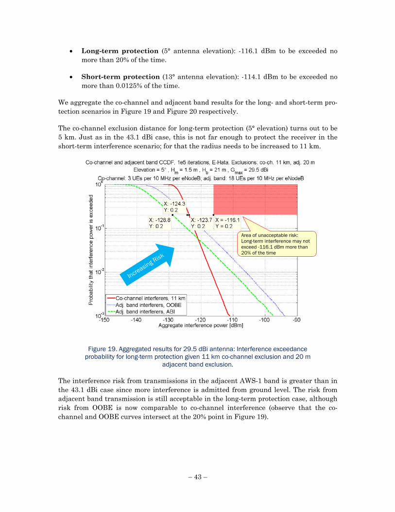
– 43 –

• Long-term protection (5° antenna elevation): -116.1 dBm to be exceeded no more than 20% of the time.

• Short-term protection (13° antenna elevation): -114.1 dBm to be exceeded no more than 0.0125% of the time.

We aggregate the co-channel and adjacent band results for the long- and short-term pro-tection scenarios in Figure 19 and Figure 20 respectively.

The co-channel exclusion distance for long-term protection (5° elevation) turns out to be 5 km. Just as in the 43.1 dBi case, this is not far enough to protect the receiver in the short-term interference scenario; for that the radius needs to be increased to 11 km.

Figure 19. Aggregated results for 29.5 dBi antenna: Interference exceedance probability for long-term protection given 11 km co-channel exclusion and 20 m

adjacent band exclusion.

The interference risk from transmissions in the adjacent AWS-1 band is greater than in the 43.1 dBi case since more interference is admitted from ground level. The risk from adjacent band transmission is still acceptable in the long-term protection case, although risk from OOBE is now comparable to co-channel interference (observe that the co-channel and OOBE curves intersect at the 20% point in Figure 19).

Area of unacceptable risk: Long-term interference may not exceed -116.1 dBm more than 20% of the time

– 44 –

Figure 20. Aggregated results for 29.5 dBi antenna: Interference exceedance probability for short-term protection given 11 km co-channel exclusion, and 20 m

adjacent band exclusion.

In the short-term case, the small (5 dB) violation of the 0.0125% IPC with a 43.1 dBi an-tenna (Figure 17) becomes a significant violation with a 29.5 dBi antenna: as can be seen from Figure 20, the OOBE risk is more than 20 dB greater than the IPC of -114.1 dBm not exceeded more than 0.0125% of the time.

In summary, we find that reducing the gain from 43.1 dBi to 29.5 dBi increases the co-channel exclusion distance from 3 km to 11 km, and dramatically increases the risk of interference from adjacent band transmitters in the short-term scenario.

ii. Baseline system performance

The risk of interference to a system can only be accurately assessed in the context of the baseline performance level.

No incumbent operates in a pristine environment; a new source of interference will con-tribute to an existing inventory of non-interference hazards, as described in section 3.A.i. The magnitude of an added risk should be judged in the context of existing risks.

The anecdotal evidence of satellite image degradation noted in Section 4.A seem to sug-gest that there is a non-trivial incidence of baseline harms in the absence of the new ser-vice interference modeled in this study. We speculate that some of it may be due to vari-

Area of unacceptable risk: Short-term interference may not exceed -114.1 dBm more than 0.0125% of the time

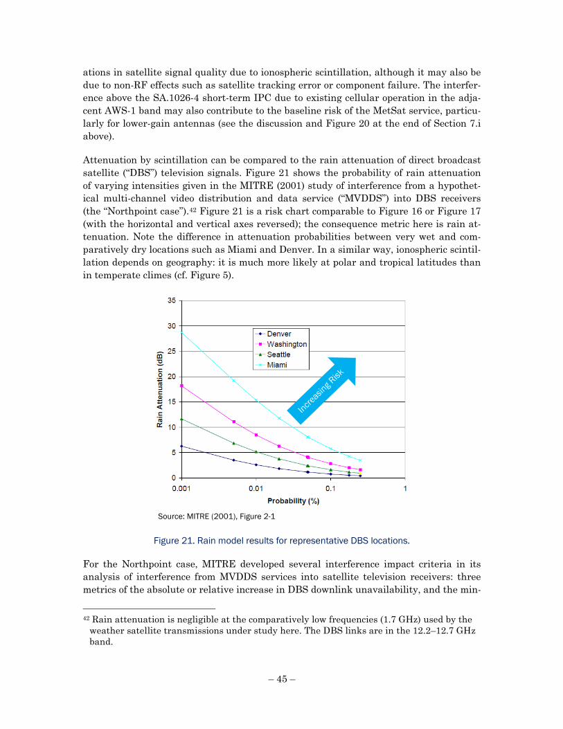
– 45 –

ations in satellite signal quality due to ionospheric scintillation, although it may also be due to non-RF effects such as satellite tracking error or component failure. The interfer-ence above the SA.1026-4 short-term IPC due to existing cellular operation in the adja-cent AWS-1 band may also contribute to the baseline risk of the MetSat service, particu-larly for lower-gain antennas (see the discussion and Figure 20 at the end of Section 7.i above).

Attenuation by scintillation can be compared to the rain attenuation of direct broadcast satellite (“DBS”) television signals. Figure 21 shows the probability of rain attenuation of varying intensities given in the MITRE (2001) study of interference from a hypothet-ical multi-channel video distribution and data service (“MVDDS”) into DBS receivers (the “Northpoint case”).42 Figure 21 is a risk chart comparable to Figure 16 or Figure 17 (with the horizontal and vertical axes reversed); the consequence metric here is rain at-tenuation. Note the difference in attenuation probabilities between very wet and com-paratively dry locations such as Miami and Denver. In a similar way, ionospheric scintil-lation depends on geography: it is much more likely at polar and tropical latitudes than in temperate climes (cf. Figure 5).

Figure 21. Rain model results for representative DBS locations.

For the Northpoint case, MITRE developed several interference impact criteria in its analysis of interference from MVDDS services into satellite television receivers: three metrics of the absolute or relative increase in DBS downlink unavailability, and the min-

42 Rain attenuation is negligible at the comparatively low frequencies (1.7 GHz) used by the

weather satellite transmissions under study here. The DBS links are in the 12.2–12.7 GHz band.

Source: MITRE (2001), Figure 2-1

– 46 –

imum clear-air value of (C/IM), where C is the weakest DBS downlink power level and IM is the MVDDS-interference power level at the output of a DBS receiving antenna (MITRE, 2001, section 5.1.1).

The most significant factor in baseline DBS unavailability is attenuation of the satellite signal due to propagation through rain. The use of an increase in DBS downlink una-vailability as an interference metric illustrates the use of baseline values by the FCC when determining interference consequences: the MVDDS rules were based on a calcu-lation that the interfering MVDDS service would increase television unavailability by no more than 10 percent over the baseline unavailability due to rain (FCC 2002, para. 71).

This principle applies in general. Interference impact should be judged in the context of baseline service degradation that occurs in the absence of added interference from a new service. In the MetSat case, Figure 20 suggests that short-term interference from exist-ing adjacent band operations can present 20 dB greater risk than that the co-channel interference level that was used to set the exclusion distance. If this adjacent band inter-ference is negligible in practice (as it seems to be), a smaller co-channel exclusion dis-tance may be justified.

iii. Mitigation

By necessity, an assessment of the risk of interference makes assumptions about the de-sign and operation of interfering transmitters and affected receivers. The outcome of the assessment may be that there will be harmful interference—but that harm may be miti-gated by changes in system parameters, for example by changes in equipment or de-ployment.

In the MetSat case, for example, we assume that the earth station receiver will absorb all interference arriving at its location. However, clutter fencing can significantly reduce the interference impinging on the antenna especially for sensitive configurations such as the 5° and 13° elevation conditions modeled above. See Figure 22 for an example of a clutter fence at a satellite downlink installation.

Mitigation can also occur at the transmitters. For example, within a specified mitigation radius, LTE UEs could not transmit on channels that overlap a MetSat channel that is in use during a satellite transit; in this case, the risk assessment would include consid-eration of adjacent channel leakage, but not co-channel interference, from UEs in the MetSat band. Another possibility would be to reduce UE maximum transmit power with-in the mitigation radius.

A mitigation that would obviate the co-channel risk analysis done in this study would be to shut down LTE operation completely during the few short time periods every day

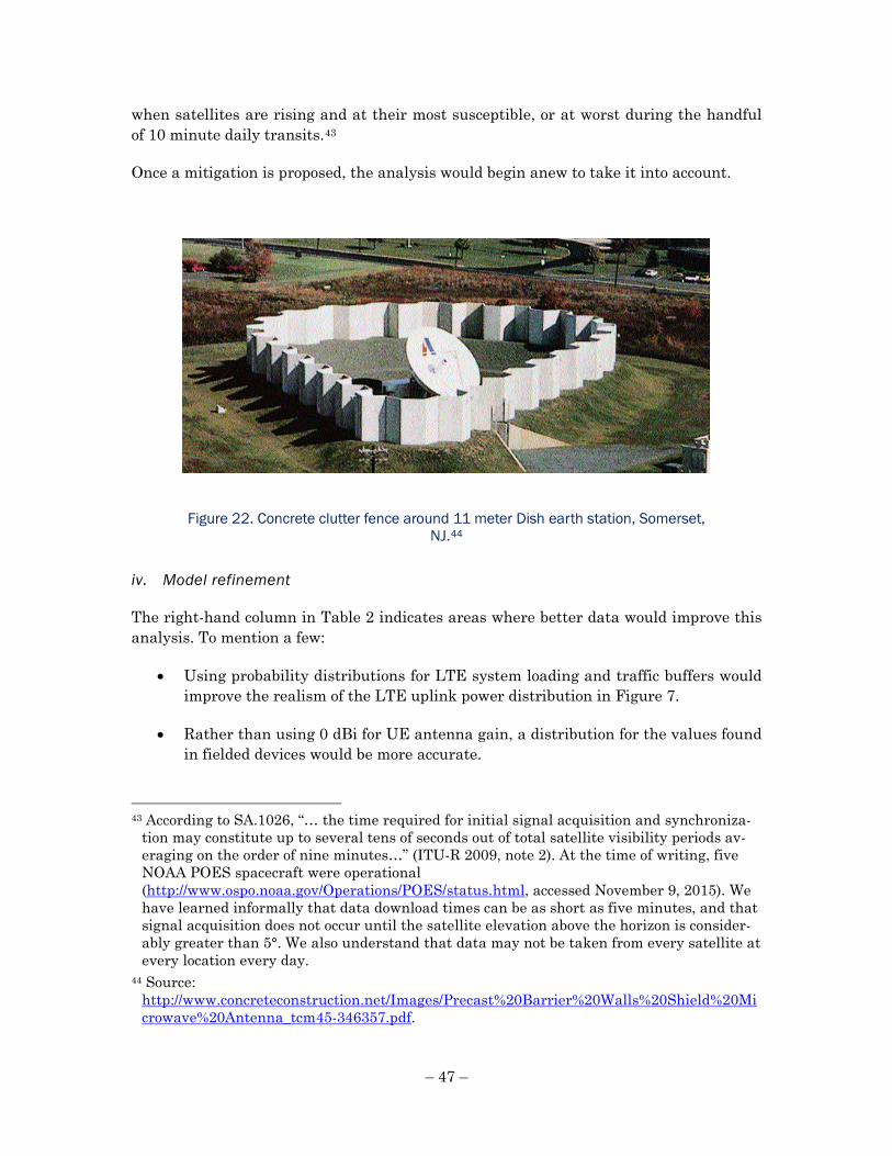
– 47 –

when satellites are rising and at their most susceptible, or at worst during the handful of 10 minute daily transits.43

Once a mitigation is proposed, the analysis would begin anew to take it into account.

Figure 22. Concrete clutter fence around 11 meter Dish earth station, Somerset, NJ.44

iv. Model refinement

The right-hand column in Table 2 indicates areas where better data would improve this analysis. To mention a few:

• Using probability distributions for LTE system loading and traffic buffers would improve the realism of the LTE uplink power distribution in Figure 7.

• Rather than using 0 dBi for UE antenna gain, a distribution for the values found in fielded devices would be more accurate.

43 According to SA.1026, “… the time required for initial signal acquisition and synchroniza-

tion may constitute up to several tens of seconds out of total satellite visibility periods av-eraging on the order of nine minutes…” (ITU-R 2009, note 2). At the time of writing, five NOAA POES spacecraft were operational (http://www.ospo.noaa.gov/Operations/POES/status.html, accessed November 9, 2015). We have learned informally that data download times can be as short as five minutes, and that signal acquisition does not occur until the satellite elevation above the horizon is consider-ably greater than 5°. We also understand that data may not be taken from every satellite at every location every day.

44 Source: http://www.concreteconstruction.net/Images/Precast%20Barrier%20Walls%20Shield%20Microwave%20Antenna_tcm45-346357.pdf.

– 48 –

• We have only studied the POES HRPT service, since we believe it to be the most interference-susceptible MetSat service in the band; other POES services, and GOES service, could also be modeled.

• A site-specific model could be developed with applicable receiver characteristics, terrain and clutter parameters, and base station deployment.

v. Consequence metrics

We modeled harm using aggregate resulting interference power as a consequence metric. As noted in Section 4, other metrics may be more informative; for example, an RF metric such as the margin consumed by interference, or service metrics such as bit-error ratio or the percentage of time the link margin is not met.

The link margin and bit-error metrics are particularly important since they would allow harm from increased interference to be put on the same footing as harm from decreased desired signal strength. Rather merely consider interference criteria (I), they also in-clude performance criteria (C/N). As suggested in a US submission to the ITU-R, it is advisable to do interference assessments by accumulating (via dynamic simulation) the statistics of C/(N+I), and to determine cumulative probability distributions of this quan-tity (USA Delegation, 2010). Bit error rates and link margin outage statistics can then be derived from C/(N+I).

vi. Peer review

Independent review of risk assessment studies is a common best practice (National Re-search Council, 2009). We have tried to facilitate review of this work by publishing the source code of the simulation model and making our spreadsheet calculations available. We look forward to feedback from the community.

– 49 –

8. Conclusions and recommendations

We conclude from this study that the method of risk-informed interference analysis pro-posed in the TAC risk paper (FCC TAC 2015) can be successfully applied in a real-world case. It yields useful insights; for example, it transpired that the binding constraint was not the long-term interference condition at 5° receiver elevation, but the short-term in-terference condition at 13°. The method can combine fixed values and probability distri-bution for interference parameters, and can combine different interference hazards (such as co-channel and adjacent band interferers) into a single risk analysis. One can incre-mentally add more sophistication such as replacing fixed values by probability distribu-tions for location variability and ACLR. We therefore recommend that the FCC pur-sue its adoption as described in the TAC risk paper.

Protection criteria that combine an interfering power level with statistical limits on how often it may be exceeded are very helpful when doing a risk-informed interference as-sessment. Such statistical interference protection criteria are already being used in a number of services, including the satellite service we analyzed and broadcast protection contours. We recommend that the FCC adopt such statistical service rules more widely in order to support future risk analysis.45

This analysis was limited by a number of factors, notably the unavailability of baseline system performance metrics. We recommend that the FCC encourage services seeking protection to disclose this information. The interference power criterion was also found to be an imperfect consequence metric, since it did not allow the long- and short-term interference scenarios to be combined into a single risk chart. It also did not shed any light on the service quality impacts of non-interference hazards such as variations in de-sired signal power or operational problems.

A final comment relates to the transparency of interference studies. In preparing this case study, we found that many of the parameter values in the ITU-R documentation are stated without explanation or backup. Those recommendations were developed for the satellite community by the satellite community. Moving forward, as risk-based interfer-ence studies are increasingly used in decision making, it is important to increase the transparency of the process and the analysis. The reproducibility, and even the credibil-ity, of such analyses can be enormously increased through a combination of transparen-cy (for example, by publishing any supporting software code) and open peer review. We recommend that the FCC encourage all parties to be as complete and transparent as possible in disclosing the methods underlying interference criteria and coexistence as-sessments.

45 While a time percentage for which interference levels may not be exceeded, such as that in

SA.1026-4, is necessary, it is arguably not sufficient: a more complete risk analysis would also need information on time scales. For example, in the MetSat case one would need to know whether interference not to be exceeded more than 0.0125% of the time should be tested over a second or a year.

– 50 –

Acknowledgments

We thank Uri Livnat for the Monte Carlo modeling reported in this paper. We are grate-ful to John Dooley, Ed Drocella, Paul McKenna, Ivan Navarro, Roger Peterson, Janne Riihijärvi, Steve Sharkey, Susan Tonkin, Jeff Ward-Bailey and the anonymous code re-viewers for their help and insight.

References

Box, G. E. P., & Draper, N. R. (1987). Empirical Model-Building and Response Surfaces. Wiley Series in Probability and Statistics. Wiley, first ed.

CSMAC (2013). Final report: Working group 1 – 1695–1710 MHz Meteorological-Satellite. Tech. rep., Commerce Spectrum Management Advisory Committee. (“WG-1 Report”). http://www.ntia.doc.gov/files/ntia/publications/wg1_report_07232013.pdf.

De Vries, J.P. (2015). Risk-informed interference assessment: A quantitative basis for spec-trum allocation decisions. In TPRC43, The research conference on communication, in-formation and internet policy. http://ssrn.com/abstract=2574459.

Drocella, E. F., Richards, J. C., Sole, R. L., Najmy, F., Lundy, A., & McKenna, P. M. (2015). 3.5 GHz exclusion zone analyses and methodology. NTIA Technical Report TR-15-517. http://www.its.bldrdoc.gov/publications/2805.aspx.

FCC (2002). Amendment of Parts 2 and 25 of the Commission’s rules to permit operation of NGSO FSS systems co frequency with GSO and terrestrial systems in the Ku band fre-quency range. Memorandum Opinion and Order and Second Report and Order. FCC 02-116, released May 23, 2002.

FCC (2014). Amendment of the Commission's rules with regard to commercial operations in the 1695-1710 MHz, 1755-1780 MHz, and 2155-2180 MHz bands. FCC-14-31.URL https://apps.fcc.gov/edocs_public/attachmatch/FCC-14-31A1.pdf.

FCC TAC (2015). A quick introduction to risk-informed interference assessment. Technical report. FCC Technological Advisory Council, Spectrum and Receiver Performance Work-ing Group. http://transition.fcc.gov/bureaus/oet/tac/tacdocs/meeting4115/Intro-to-RIA-v100.pdf.

IEEE (2008). IEEE recommended practice for the analysis of in-band and adjacent band in-terference and coexistence between radio systems. IEEE Std 1900.2-2008, IEEE Com-munications Society. http://ieeexplore.ieee.org/servlet/opac?punumber=4584233.

ITU-R (1994). Recommendation SA.1022-0 in SA.1022 : Methodology for determining inter-ference criteria for systems in the earth exploration-satellite and meteorological-satellite services. , ITU Radiocommunication Sector. https://www.itu.int/rec/R-REC-SA.1022-0-199403-S/en.

ITU-R (1999). Recommendation SA 1025-3, in SA. 1025 : Performance criteria for space-to-Earth data transmission systems operating in the Earth exploration-satellite and mete-orological-satellite services using satellites in low-Earth orbit. ITU Radiocommunication Sector. https://www.itu.int/rec/R-REC-SA.1025-3-199910-I/en.

ITU-R (2009). Recommendation SA.1026-4, in SA.1026 : Aggregate interference criteria for space-to-earth data transmission systems operating in the earth exploration-satellite and meteorological-satellite services using satellites in low-Earth orbit. ITU Radiocom-munication Sector. http://www.itu.int/rec/R-REC-SA.1026-4-200902-I/en.

ITU-R (2012). Recommendation F.1245-2, in F.1245 : Mathematical model of average and related radiation patterns for line-of-sight point-to-point fixed wireless system antennas for use in certain coordination studies and interference assessment in the frequency

– 51 –

range from 1 GHz to about 70 GHz. ITU Radiocommunication Sector. https://www.itu.int/rec/R-REC-F.1245/en.

Kaplan, S. & Garrick, B. J. (1981). On the quantitative definition of risk. Risk Analysis, 1(1):11-27. http://dx.doi.org/10.1111/j.1539-6924.1981.tb01350.x.

Longley, A. G. (1978). Radio propagation in urban areas. Technical Report, OT Report 78-144, U.S. Department of Commerce. http://www.its.bldrdoc.gov/publications/2674.aspx.

National Research Council (2009). Science and decisions: Advancing risk assessment. The National Academies Press. http://www.nap.edu/catalog/12209/science-and-decisions-advancing-risk-assessment.

NTIA (2010). An assessment of the near-term viability of accommodating wireless broadband systems in the1675–1710 MHz, 1755–1780 MHz, 3500–3650 MHz, 4200–4220 MHz, and 4380–4400 MHz bands (“Fast Track Report”). Technical report, U.S. Department of Commerce. http://www.ntia.doc.gov/files/ntia/publications/fasttrackevaluation_11152010.pdf.

Ofcom (2012). LTE user equipment: Coexistence with 862 - 870MHz. Technical report, Ofcom. URL http://stakeholders.ofcom.org.uk/binaries/consultations/award-800mhz/statement/lte-coexistence.pdf.

Sanders, F. H., Sole, R. L., Bedford, B. L., Franc, D., & Pawlowitz, T. (2006). Effects of RF interference on radar receivers. Technical report TR-06-444, NTIA ITS. http://www.its.bldrdoc.gov/publications/06-444.aspx.

TR46 (2001). Licensed PCS to PCS interference. Technical report TSB-84A, TIA/EIA. USA Delegation (2007). The use of short term probabilities in interference criteria docu-

ments, with a preliminary draft revision to recommendation ITU-R SA.1026-3. Docu-ment 7B/159-E, ITU Radiocommunication Study Groups. https://www.itu.int/md/R07-WP7B-C-0159/en.

USA Delegation (2010). Working document toward a preliminary draft new recommendation ITU-R SA.[EES/MET PERF]: MetSat and EESS performance objectives in the presence of interference. ITU-R WP7B Contribution 235, ITU Radiocommunication Study Groups. https://www.itu.int/md/R07-WP7B-C-0235/en.

– 52 –

Appendix 1: Monte Carlo Model

The following MATLAB code (Version 3) was used to generate the results reported in this report.

SimulCoCh.m %{ Related documents for the simulation (1) http://www.its.bldrdoc.gov/publications/2805.aspx relevant part is Appendix A, equations 1-14 (2) http://www.ntia.doc.gov/files/ntia/publications/wg_1_report.pdf Relevant parts are Appendix 3 and 7 General explanation of code: The XY plane is divided to Suburban and rural deployments, according to the distance from (0,0). Suburban and rural deployments vary in density and transmitting power of the UEs. 1. An inner ring around (0,0) between Dmin(1) and Dmax(1) contains sub-urban deployments and the outer ring between Dmin(2) and Dmax(2) contains rural deployments. At each ring, UEs are uniformly distributed accord-ing to a predefined density. 2. from Dmin(1) to Dmax(2), for each 1km interval, per iteration out of N iterations : a. UEs are randomly deployed b. Received power (=interference) in (0,0) is calculated, given the 'contribution' of each UE in the domain. c. Repeat a-c unless maximum amount of iterations is reached, then 1 km is reduced from the inner ring and 2 is repeated 3. Received power is calculated as: P(Rx) = sum [ P(Tx) - L + G + SF - RxL - OTR] Where: L is the pathloss which is calculated according to document (1) in the list G is the antenna gain according to SF is Shadow Fading, lognormally distributed RxL is Rx Losses, predefined fixed value OTR is On Tune Rejection, predefined fixed value XYmat:

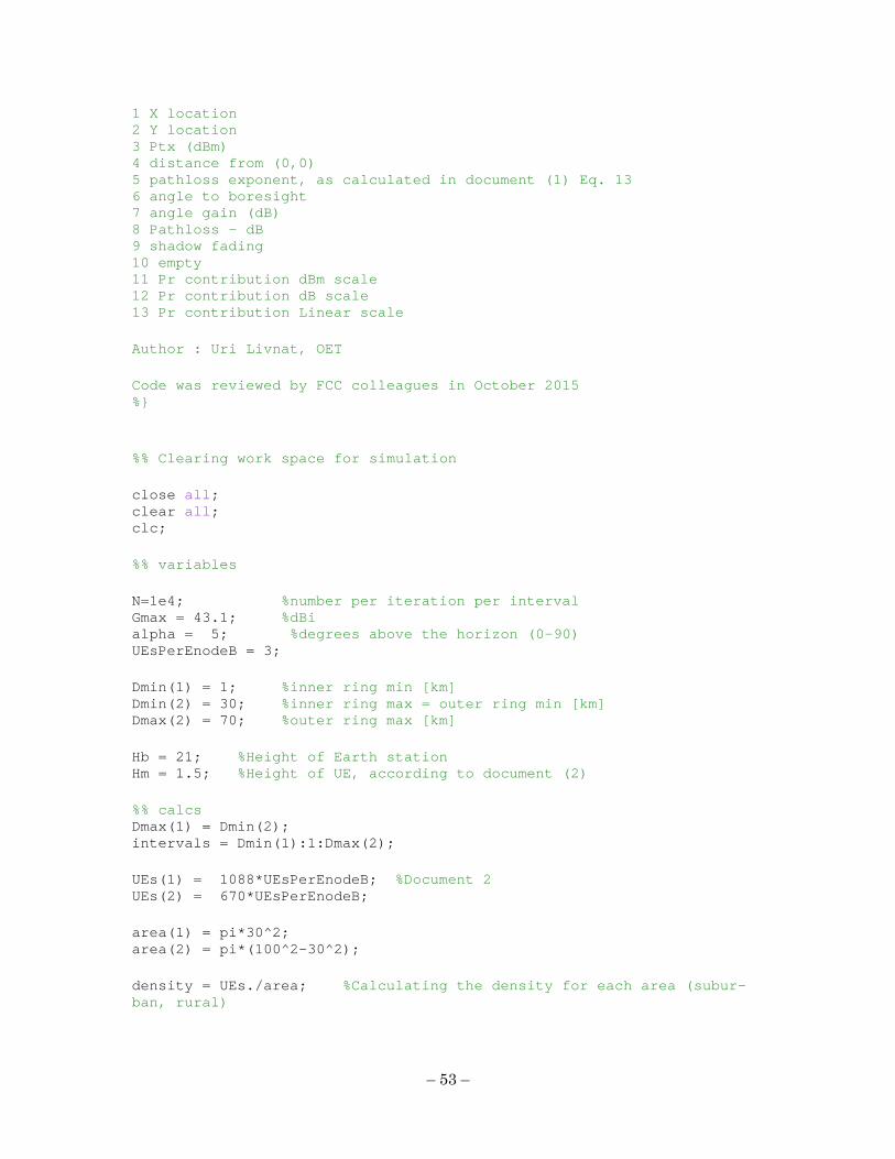
– 53 –

1 X location 2 Y location 3 Ptx (dBm) 4 distance from (0,0) 5 pathloss exponent, as calculated in document (1) Eq. 13 6 angle to boresight 7 angle gain (dB) 8 Pathloss - dB 9 shadow fading 10 empty 11 Pr contribution dBm scale 12 Pr contribution dB scale 13 Pr contribution Linear scale Author : Uri Livnat, OET Code was reviewed by FCC colleagues in October 2015 %} %% Clearing work space for simulation close all; clear all; clc; %% variables N=1e4; %number per iteration per interval Gmax = 43.1; %dBi alpha = 5; %degrees above the horizon (0-90) UEsPerEnodeB = 3; Dmin(1) = 1; %inner ring min [km] Dmin(2) = 30; %inner ring max = outer ring min [km] Dmax(2) = 70; %outer ring max [km] Hb = 21; %Height of Earth station Hm = 1.5; %Height of UE, according to document (2) %% calcs Dmax(1) = Dmin(2); intervals = Dmin(1):1:Dmax(2); UEs(1) = 1088*UEsPerEnodeB; %Document 2 UEs(2) = 670*UEsPerEnodeB; area(1) = pi*30^2; area(2) = pi*(100^2-30^2); density = UEs./area; %Calculating the density for each area (subur-ban, rural)

– 54 –

beta = 0; %degrees on the XY plane (0-360) SFmean = 0 ; %Shadow Fading mean value in dB - lognormal distribu-tion with : SF ~ logN(SFmean,SFsigma) SFsigma = 8 ; %Shadow Fading sigma value in dB f = 1707e6; %Carrier Freq in Hz RxL = 1; %Rx loss in dB OTR = 0.5; %OTR loss in dB DoverLambda = 10^((Gmax-7.7)/20); %% calcs a_rad = pi*alpha/180; %alpha in radians b_rad = pi*beta/180; %beta in radians ESxyz = [cos(a_rad)*cos(b_rad),cos(a_rad)*sin(b_rad) ,sin(a_rad)]; %projections of vector on axis x y z %% finding constants for EHata, according to document (1) %parameters name match these in document (1) nl = 0.1*(24.9-6.55*log10(Hb)); %Eq. 7 nh = (-0.75 + 3.27*log10(Hb) - 0.67*(log10(Hb)).^2 - 1)*2; %Eq. 7 Abm1 = 30.52 - 16.81*log10(f/1e6) + 4.45*(log10(f/1e6)).^2 + 9.83*log10(1); %Eq. 6 @ 1 km Abm100 = 120.78 - 52.71*log10(f/1e6) + 10.92*(log10(f/1e6)).^2 ; %@ 100 km abm1 = 10^(Abm1/10); %Abm = 10log(abm) abm100 = 10^(Abm100/10); Dbp = (10^(2*nh)*(abm1/abm100))^(1/(nh-nl)); %9b Abm = 30.52 - 16.81*log10(f/1e6) + 4.45*(log10(f/1e6))^2 + (24.9 - 6.55*log10(Hb))*log10(Dbp); %11 a3 = 3.2*(log10(11.75*3))^2-4.97; %2a ahm = 3.2*(log10(11.75*Hm))^2-4.97; %2a %% sampling Tx powers from pdf, according to document (2) %CDF range and steps xqR = -40 : 3 : 20; xqU = -40 : 3 : 20; %cdf values for rural and suburban UEs

– 55 –

cdfR = [0 0 0 0 0 0 0.0002 0.0006 0.0013 0.0039 0.0099 0.0252 0.0577 0.1152 0.2062 0.3307 0.4843 0.6448 0.7920 0.9123 1.0000]; cdfU = [0 0.0001 0.0003 0.0011 0.0031 0.0071 0.0154 0.0320 0.0647 0.1194 0.2033 0.3160 0.4530 0.5959 0.7297 0.8390 0.9143 0.9594 0.9830 0.9936 1.0000]; [cdfR, maskR] = unique(cdfR); xqR = xqR(maskR); [cdfU, maskU] = unique(cdfU); xqU = xqU(maskU); results = zeros (length(intervals)-1,N); normESxyz = norm(ESxyz); %upper bound of 'for loop' can be modified for 13 degrees case. for j = 1:(length(intervals)-1) j for iter = 1:N if (mod(iter,2000) == 0) %easier to follow progress on MATLAB command window tool iter end clear XYmat; if intervals(j)<Dmin(2) %suburban and rural deploymetns XYmat1 = ring(intervals(j),Dmax(1),density(1)); %suburban XYmat2 = ring(Dmin(2),Dmax(2),density(2)); %rural XYmat = [XYmat1 ; XYmat2]; %concate-nation of matrices clear XYmat1; clear XYmat2; else XYmat = ring(intervals(j),Dmax(2),density(2)); %rural on-ly end % finding the angle between 2 vectors CosT = dot(XYmat(:,1:3),repmat(ESxyz,length(XYmat(:,1)),1),2)./(sqrt(XYmat(:,1).^2+XYmat(:,2).^2+XYmat(:,3).^2)*normESxyz); thet = acos(CosT')*180/pi; %Theta XYmat(:,6)=thet'; clear thet; clear CosT; XYmat(:,7) = CFR(XYmat(:,6),DoverLambda); %% borderindex = find (XYmat(:,4)>Dmin(2)*1e3); %checking whether there are suburban deployments or just rural (depends on distance) if (borderindex(1)-1) %there are subur-ban deployments randomValues1 = rand(1,(borderindex(1)-1));

– 56 –

XYmat(1:(borderindex(1)-1),3) = interp1(cdfU, xqU, ran-domValues1); %dBm randomValues2 = rand(1,length(borderindex)); XYmat(borderindex(1):end,3) = interp1(cdfR, xqR, ran-domValues2); %dBm clear randomValues1; clear randomValues2; else %no suburban deployments randomValues = rand(1,length(borderindex)); XYmat(borderindex(1):end,3) = interp1(cdfR, xqR, randomValues); %dBm clear randomValues; end; rn = find(XYmat(:,4)>Dbp*1e3); %Eq. 13 - 2 slopes approach if (rn(1)-1) %there are deployments below Dbp XYmat(1:(rn(1)-1),5) = 0.1*(24.9 - 6.55*log10(Hb)); XYmat(rn(1):end,5) = 2*(3.27*log10(Hb) - 0.67*(log10(Hb))^2 - 1.75); else %no deployments below Dbp XYmat(rn(1):end,5) = 2*(3.27*log10(Hb) - 0.67*(log10(Hb))^2 - 1.75); end; XYmat(:,9) = normrnd(SFmean,SFsigma,1,length(XYmat(:,1))); %Shadow fading In dB Lfs = 20*log10(4*pi*(XYmat(:,4))/300) + 20*log10(f/1e6); %docu-ment (1) Eq. 4d XYmat(:,8) = Abm + 10*XYmat(:,5).*log10((XYmat(:,4)/1e3)/Dbp) + 13.82*log10(200/Hb) + a3 - ahm + Lfs; %Eq. 10 XYmat(:,8) = XYmat(:,8) - (54.19 - 33.3*log10(f/1e6) + 6.25*(log10(f/1e6))^2); %suburban correction factor XYmat(:,11) = XYmat(:,3) - XYmat(:,8) + XYmat(:,7) + XYmat(:,9) - RxL - OTR; %link budget. result is in dBm XYmat(:,12) = XYmat(:,11) - 30; %in dB XYmat(:,13) = 10.^(XYmat(:,12)./10); %linear Ptot = sum (XYmat(:,13)); %total received power on linear scale results(j,iter) = Ptot; end end if (j==1) %used for plotting the CDFs of the actual UEs in the simula-tion

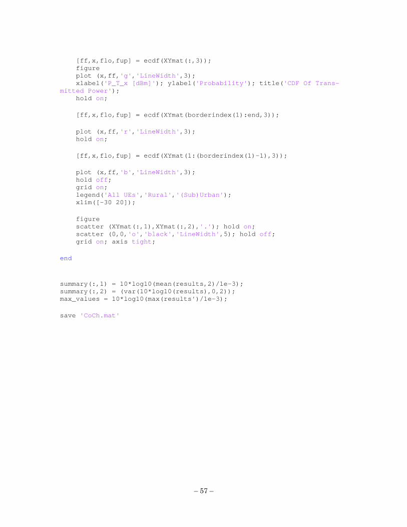
– 57 –

[ff,x,flo,fup] = ecdf(XYmat(:,3)); figure plot (x,ff,'g','LineWidth',3); xlabel('P_T_x [dBm]'); ylabel('Probability'); title('CDF Of Trans-mitted Power'); hold on; [ff,x,flo,fup] = ecdf(XYmat(borderindex(1):end,3)); plot (x,ff,'r','LineWidth',3); hold on; [ff,x,flo,fup] = ecdf(XYmat(1:(borderindex(1)-1),3)); plot (x,ff,'b','LineWidth',3); hold off; grid on; legend('All UEs','Rural','(Sub)Urban'); xlim([-30 20]); figure scatter (XYmat(:,1),XYmat(:,2),'.'); hold on; scatter (0,0,'o','black','LineWidth',5); hold off; grid on; axis tight; end summary(:,1) = 10*log10(mean(results,2)/1e-3); summary(:,2) = (var(10*log10(results),0,2)); max_values = 10*log10(max(results')/1e-3); save 'CoCh.mat'

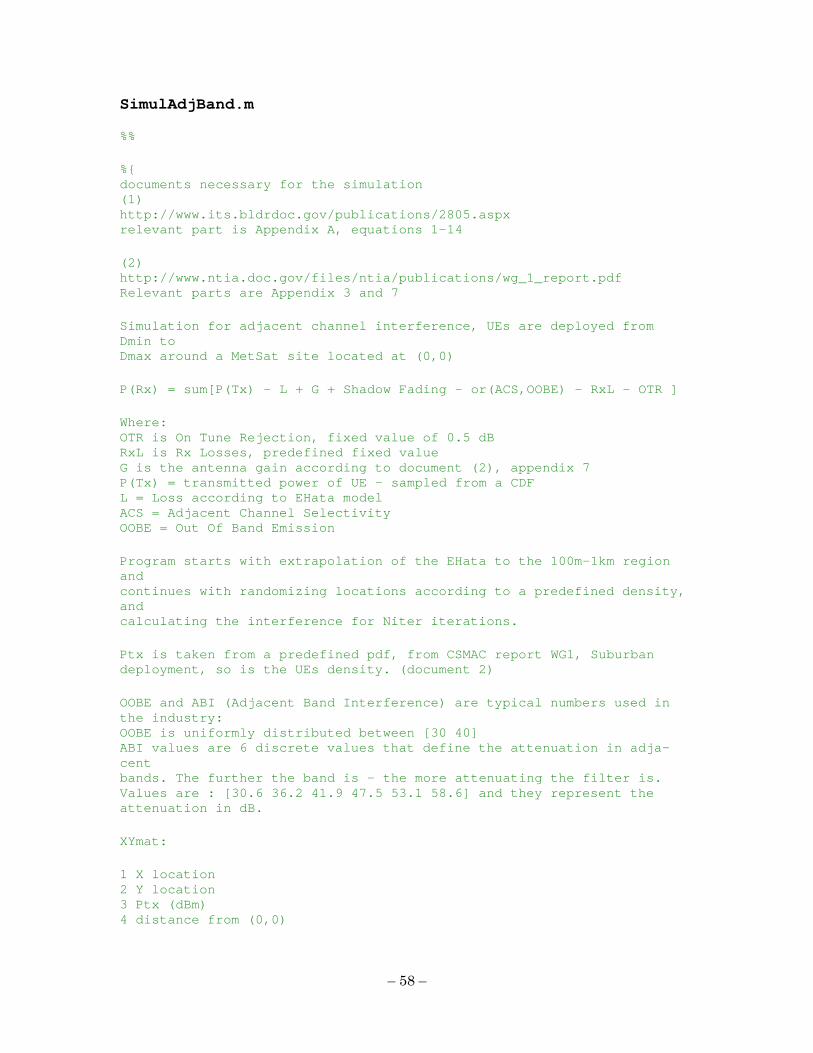
– 58 –

SimulAdjBand.m %% %{ documents necessary for the simulation (1) http://www.its.bldrdoc.gov/publications/2805.aspx relevant part is Appendix A, equations 1-14 (2) http://www.ntia.doc.gov/files/ntia/publications/wg_1_report.pdf Relevant parts are Appendix 3 and 7 Simulation for adjacent channel interference, UEs are deployed from Dmin to Dmax around a MetSat site located at (0,0) P(Rx) = sum[P(Tx) - L + G + Shadow Fading - or(ACS,OOBE) - RxL - OTR ] Where: OTR is On Tune Rejection, fixed value of 0.5 dB RxL is Rx Losses, predefined fixed value G is the antenna gain according to document (2), appendix 7 P(Tx) = transmitted power of UE - sampled from a CDF L = Loss according to EHata model ACS = Adjacent Channel Selectivity OOBE = Out Of Band Emission Program starts with extrapolation of the EHata to the 100m-1km region and continues with randomizing locations according to a predefined density, and calculating the interference for Niter iterations. Ptx is taken from a predefined pdf, from CSMAC report WG1, Suburban deployment, so is the UEs density. (document 2) OOBE and ABI (Adjacent Band Interference) are typical numbers used in the industry: OOBE is uniformly distributed between [30 40] ABI values are 6 discrete values that define the attenuation in adja-cent bands. The further the band is - the more attenuating the filter is. Values are : [30.6 36.2 41.9 47.5 53.1 58.6] and they represent the attenuation in dB. XYmat: 1 X location 2 Y location 3 Ptx (dBm) 4 distance from (0,0)

– 59 –

5 OOBE or ABI (Adjacent band interference) value 6 angle to boresight 7 angle gain (dB) 8 Pathloss - dB 9 shadow fading 10 pathloss exponent 11 Pr contribution dBm scale 12 Pr contribution dB scale 13 Pr contribution Linear scale Author : Uri Livnat, OET Code was reviewed by FCC colleagues in October 2015 %} clc; close all; clear all; %% Programmable Parameters Niter=1e5; %number per iteration per interval Dmin = 0.02; %inner ring min [km] Dmax = 20; %inner ring max = outer ring min [km] Gmax = 43.1; %FSS receiver antenna gain [dBi] alpha = 5; %boresight degrees above the horizon (0-90) f = 1707e6; %Carrier Freq %% Const Parameters Hb = 21; %Height of Earth station Hm = 1.5; %Height of UE, according to document (2) D=1:0.1:100; %km beta = 0; %degrees on the XY plane (0-360) UEsPerEnodeB = 18; SFmean = 0; SFsigma = 8; %in dB RxL = 1; %Rx Losses are predefined and equal to 1 dB OTR = 0.5; %OTR loss in dB ABIv = [30.6 36.2 41.9 47.5 53.1 58.6]; %Adjacent Band Interference Discrete Values %% finding constants for EHata, according to document (1) % parameters notations match those in document (1)

– 60 –

n1 = 0.1*(24.9 - 6.55*log10(Hb)); %pathloss exponent up to Dbp. Eq 13 n2 = 2*(3.27*log10(Hb) - 0.67*(log10(Hb))^2 - 1.75);; %pathloss expo-nent above Dbp. Eq 13 nl = 0.1*(24.9-6.55*log10(Hb)); %Eq. 7 nh = (-0.75 + 3.27*log10(Hb) - 0.67*(log10(Hb)).^2 - 1)*2; %Eq. 7 Abm1 = 30.52 - 16.81*log10(f/1e6) + 4.45*(log10(f/1e6)).^2 + 9.83*log10(1); %Eq. 6 @ 1 km Abm100 = 120.78 - 52.71*log10(f/1e6) + 10.92*(log10(f/1e6)).^2 ; %@ 100 km abm1 = 10^(Abm1/10); %Abm = 10log(abm) abm100 = 10^(Abm100/10); Dbp = (10^(2*nh)*(abm1/abm100))^(1/(nh-nl)); %9b Abm = 30.52 - 16.81*log10(f/1e6) + 4.45*(log10(f/1e6))^2 + (24.9 - 6.55*log10(Hb))*log10(Dbp); %11 a3 = 3.2*(log10(11.75*3))^2-4.97; %2a ahm = 3.2*(log10(11.75*Hm))^2-4.97; %2a Lfs = 20*log10(4*pi*D*1e3/300) + 20*log10(f/1e6); %document (2) Eq. 4d, D is in meters Lp = Abm + 10*n1.*log10(D/Dbp) + 13.82*log10(200/Hb) + a3 - ahm + Lfs; %Eq. 10 (used for deployments up to 1km, therefore n1 is used) Lps = Lp - (54.19 - 33.3*log10(f/1e6) + 6.25*(log10(f/1e6))^2); %suburban correction factor %% FreeSpacePathLoss20m = 20*log10(20) + 20*log10(f) - 147.55 ; %Free Space pathloss value @ 20 meters InterpValsX = 0.02:0.001:1; %interpolation values : from 20 meters to 1 km, in 1m increments InterpBoundsX = log10([20 1000]*1e-3); %interpolation lower and up-per bound, in km. AttenInterpValsY = interp1(InterpBoundsX,[FreeSpacePathLoss20m Lps(1)],log10(InterpValsX),'linear'); %Interpolation to find attenu-ation values, per meter, in dB SFInterpValsY = interp1(InterpBoundsX,[0 SFsig-ma],log10(InterpValsX),'linear'); %Interpola-tion to find shadow Fading values, per meter, in dB %% calcs a_rad = pi*alpha/180; %alpha in radians b_rad = pi*beta/180; %beta in radians

– 61 –

ESxyz = [cos(a_rad)*cos(b_rad),cos(a_rad)*sin(b_rad) ,sin(a_rad)]; %projections of vector on axis [x y z] SuburbanCDF = [0 0.0001 0.0003 0.0011 0.0031 0.0071 0.0154 0.0320 0.0647 0.1194 0.2033 0.3160 0.4530 0.5959 0.7297 0.8390 0.9143 0.9594 0.9830 0.9936 1.0000]; SuburbanPtxValuesCDF = -40 : 3 : 20; %Transmition Power values which correspond to CDF values normESxyz = norm(ESxyz); %Norm value of Earth Station antenna vector DoverLambda = 10^((Gmax-7.7)/20); area = pi*30^2; %Used for density calculation UEs = 1088*UEsPerEnodeB; density = UEs/area; %% results = zeros (1,Niter); for OOBE = 0:1 %one run for both independent simulations - for j = 1:Niter clear XYmat if mod(j,1000) == 0 j %to see simulation progress end XYmat = ring(Dmin,Dmax,density); %Deploying UEs between <Dmin> and <Dmax> with density <density> XYmat(:,4) = sqrt(XYmat(:,4).^2+(Hb-Hm)^2); %not negligible in small distances XYmat(:,4) = round(XYmat(:,4)); %precision is to 1 meter, used later for look up tables for the attenuation and Shadow Fading value (up to 1000m) CosT = dot(XYmat(:,1:3),repmat(ESxyz,size(XYmat,1),1),2)./(sqrt(XYmat(:,1).^2+XYmat(:,2).^2+XYmat(:,3).^2)*normESxyz); %finding the angle between 2 vectors thet = acos(CosT')*180/pi; %Theta - angle between 2 vectors. In our case - between the boresight and the UE location XYmat(:,6)=thet'; XYmat(:,7) = CFR(XYmat(:,6),DoverLambda); if OOBE %OOBE XYmat(:,5) = rand(1,size(XYmat,1))*10+30; %OOBE [30 40] else %ACS ABIind = ceil(rand(1,size(XYmat,1))*(length(ABIv))); %ABI index XYmat(:,5) = ABIv(ABIind); end randomValues = rand(1,size(XYmat,1));

– 62 –

XYmat(:,3) = interp1(SuburbanCDF, SuburbanPtxValuesCDF, ran-domValues); %dBm, Tx Power Lfsi = 20*log10(4*pi*(XYmat(:,4))/300) + 20*log10(f/1e6); %document (2) Eq. 4d %% rn = find(XYmat(:,4)>Dbp*1e3); %Eq. 13 - 2 slopes approach XYmat(1:(rn(1)-1),10) = n1; %pathloss exponent below Dbp XYmat(rn(1):end,10) = n2; %pathloss exponent above Dbp ind = find(XYmat(:,4)>1e3); %above 1000m - regular treatment XYmat(ind,8) = Abm + 10*(XYmat(ind,10)).*log10((XYmat(ind,4)/1e3)/Dbp) + 13.82*log10(200/Hb) + a3 - ahm + Lfsi(ind); %Eq. 10 XYmat(ind,8) = XYmat(ind,8) - (54.19 - 33.3*log10(f/1e6) + 6.25*(log10(f/1e6))^2); %suburban correction factor XYmat(ind,9) = normrnd(SFmean,SFsigma,1,length(ind)); %Shadow fading In dB for i=1:ind(1)-1 %under 1000m - special treatment indlow = find(InterpValsX*1e3 >= XYmat(i,4)); %Find-ing the corresponding index for the distance to use in lookup tables: XYmat(i,8) = AttenInterpValsY(indlow(1)); %Cor-responding attenuation XYmat(i,9) = normrnd(SFmean,SFInterpValsY(indlow(1)),1,1); %corresponding shadow fading end XYmat(:,11) = XYmat(:,3) - XYmat(:,8) + XYmat(:,7) + XYmat(:,9) - XYmat(:,5) - OTR - RxL; %link budget. result is in dBm XYmat(:,12) = XYmat(:,11) - 30; %in dB XYmat(:,13) = 10.^(XYmat(:,12)./10); %linear results(j) = sum(XYmat(:,13)); end if OOBE save 'OOBE.mat' else save 'ACS.mat' end end

– 63 –

%% plotting figure scatter (XYmat(:,1),XYmat(:,2),'.'); hold on; scatter (0,0,'o','black','LineWidth',5); hold off; grid on; axis tight;

– 64 –

ring.m function [ XYmat ] = ring( Dmin , Dmax ,dense ) %function to create uniform random distribution of XY points in the ring %with Dmin,Dmax and density %Dmin and Dmax is in km %dense is [cells/km^2] NUEs = round(dense*(Dmax*2)^2); %Density*area XYmat(:,1:2) = (rand(NUEs,2)-0.5)*2*1e3*Dmax; %in meters temp = sqrt(XYmat(:,1).^2+XYmat(:,2).^2); XYmat(:,4) = temp'; [values, order] = sort(XYmat(:,4)); XYmat = XYmat(order,:); row = find(and(XYmat(:,4)>=Dmin*1e3,XYmat(:,4)<=Dmax*1e3)); clear temp; temp=XYmat(row(1):row(end),:); clear XYmat; XYmat=temp; end CFR.m function [ VECout ] = CFR( VECin, DoverLambda ) %calculates the gain per angle %VECin is the angles vector - input to function %VECout is the gains vector - output of function %D is Diameter of Antenna %Lambda = c/f %D over Lambda is used for gain calculations %lowest possible angle as input is 1.5 degrees VECout = zeros(length(VECin),1); k = find(and(VECin>=1.5,VECin<=48)); VECout(k) = 39-5*log10(DoverLambda)-25*log10(VECin(k)); k1 = find(VECin>48); VECout(k1) = -3-5*log10(DoverLambda); VECout = VECout'; distXY.m function [ Dist ] = distXY(UsersMat,ES) Dist(:) = sqrt((UsersMat(:,1) - ES(1))^2 + (UsersMat(:,2) - ES(2))^2);