J. Parallel Distrib. Comput. 71 (2011) 556–564

Contents lists available at ScienceDirect

J. Parallel Distrib. Comput.

journal homepage: www.elsevier.com/locate/jpdc

A case for on-machine load balancingShoukat Ali a,∗, Behdis Eslamnour b, Zehra Shah c

a Platform Validation Enabling, Intel Corporation, Folsom, CA 95630, USAb Department of Electrical and Computer Engineering, Missouri University of Science and Technology, Rolla, MO 65409-0040, USAc Department of Computer Science, Lahore University of Management Sciences, Lahore, Pakistan

a r t i c l e i n f o

Article history:Received 5 July 2009Received in revised form29 September 2010Accepted 5 November 2010Available online 21 November 2010

Keywords:Load balancing and task assignmentApplication studies resulting in bettermultiple-processor systems

Measurement, evaluation, modeling,simulation of multiple-processor systems

Resource allocation

a b s t r a c t

This paper diverges from the traditional load balancing, and introduces a new principle called the on-machine load balance rule. The on-machine load balance rule leads to resource allocations that are better intolerating uncertainties in the processing times of the tasks allocated to the resources when compared toother resource allocations that are derived using the conventional ‘‘across-the-machines’’ load balancingrule. The on-machine load balance rule calls for the resource allocation algorithms to allocate similarlysized tasks on a machine (in addition to optimizing some primary performance measures such asestimatedmakespan and average response time). The on-machine load balance rule is very different fromthe usual across-the-machines load balance rule that strives to balance load across resources so that allresources have similar finishing times.

We give a mathematical justification for the on-machine load balance rule requiring only liberalassumptions about task processing times. Then we validate with extensive simulations that the resourceallocations derived using on-machine load balance rule are indeed more tolerant of uncertain taskprocessing times.

© 2010 Elsevier Inc. All rights reserved.

1. Introduction

This paper makes a case for a new concept we have named asthe on-machine load balance rule. We will show that using the on-machine load balance rule to guide search heuristics usually leadsto resource allocations that are better in tolerating uncertainties inthe processing times of the taskswhen compared to other resourceallocations that are derived using the conventional ‘‘across themachines’’ load balancing rule. We formally state the rule asfollows.

On-Machine Load Balance Rule:For two computing nodes that have the same estimated finishingtime, and the same deadline before which the nodes must processtheir load, the node that has a larger number of tasks and moreequally sized tasksmapped on it is less likely to violate the deadline.

We also state the following two special cases of the on-machineload balance rule.1: For two computing nodes that have an equal number of tasksallocated to them, have the same estimated finishing time, and the

∗ Corresponding address: Exascale Stream Computing Collaboratory, SmarterCities Technology Center, IBM Research, Dublin, Ireland.

E-mail addresses: shoukat.ali@intel.com, drshoukatali@gmail.com,alishou8@ie.ibm.com (S. Ali), ben88@mst.edu (B. Eslamnour),zehra.hasanain@gmail.com (Z. Shah).

0743-7315/$ – see front matter© 2010 Elsevier Inc. All rights reserved.doi:10.1016/j.jpdc.2010.11.003

same deadline before which the nodes must process their load, thenodewhere the tasks aremore similarly sized is less likely to violatethe deadline.2: For two computing nodes that have a number of equally sizedtasks allocated to them, have the same estimated finishing time,and the same deadline before which the nodes must process theirload, the node that has a larger number of tasks mapped on it isless likely to violate the deadline.

The on-machine load balance rule calls for the resourceallocation algorithms to allocate similarly sized tasks on amachine(in addition to optimizing some primary performance measuresuch as estimated makespan and average response time). Our on-machine load balance rule is very different from the usual across-the-machines load balance rule that strives to balance load acrossmachines so that all machines have similar finishing times.Wewillshow in this paper that the resource allocations derived using theon-machine load balance rule are less likely to violate a deadlineplaced on the overall completion time of the set of tasks than otherresource allocations that have not followed the on-machine loadbalance rule, even if they still have the same estimated makespan.

Note that the design of an actual resource allocation heuristic isnot the subject of this paper. That topic is addressed in a numberof other papers (e.g., [3,6,5,13,28,30,32,48]). The subject is to showwhat makes resource allocations ‘‘robust’’ against task processingtime uncertainties. This knowledge can then be used to guide thesearch in resource allocation heuristics.

S. Ali et al. / J. Parallel Distrib. Comput. 71 (2011) 556–564 557

a b

Fig. 1. Each bar in this figure shows the finishing time for amachine, and is split into asmanypieces as the number of applications on themachine. The tasks and themachinesare heterogeneous. The heterogeneity of machines implies that different nodes take different processing times for a given task. Similarly task heterogeneity implies thatdifferent tasks take different processing times on a given node.

Tomotivate further discussion, let us pick a running example ofa cluster of five heterogeneous computing nodes that are expectedto execute a set of 20 heterogeneous non-communicating tasks.Now consider the two resource allocations in Fig. 1 that havebeen derived for this system. Each bar in this figure shows thefinishing time for a machine, and is split into as many piecesas the number of applications on the machine. The tasks andthe machines are heterogeneous. The heterogeneity of machinesimplies that different nodes take different processing times for agiven task. Similarly task heterogeneity implies that different taskstake different processing times on a given node. No assumptionsabout task or machine homogeneity have been made in thisresearch.

Considering only the estimated makespan (i.e., the estimatedtime taken for the entire set of tasks to finish processing) as theperformance measure, one would consider both of these resourceallocations to be equally desirable. Considering both estimatedmakespan and across-the-nodes load balance (measured here bythe standard deviation of the finishing times of the five computingnodes), one would actually prefer resource allocation in Fig. 1(a)because it has a better across-the-nodes load balance.

Now assume that one requirement for this system is thatthe estimated makespan not exceed a pre-declared deadline. Thepurpose of this paper is to show that in the event of actual taskprocessing times being different from the estimated ones, theactual makespan of the resource allocation in Fig. 1(b) is morelikely to stay below the deadline than the actual makespan of theresource allocation given in Fig. 1(a). We will further show thatthis ‘‘robustness’’ of resource allocation in Fig. 1(b) is caused bybetter ‘‘on-machine load balancing’’ on its node 3 as compared tothe similarly loaded node 4 in resource allocation 1(a). By betteron-machine load balancing, we specifically mean that the six taskson node 3 in 1(b) are more similarly sized than the six tasks onnode 4 in 1(a). We say that the total computational load on node 3in 1(b) is more well balanced than the similar total computationalload on node 4 in 1(a). This concept of load balancing within anode is very different from the usual notion of ‘‘across-the-nodesload balancing’’ that strives to equalize the finishing times of allnodes. We will show in this paper that the better on-machine loadbalance for the resource allocation in Fig. 1(b) leads to a higherprobability of its actualmakespan staying below the given deadlinein the event of actual task processing times being different from theestimated ones.

Although this paper will use a working example of a clustercomputing system to expose the concepts, the results are broadlyapplicable. The on-machine load balance rule could be applied

to enhance the tolerance of, for example, a power grid againstfluctuations in the load and that of networks against variations inthe traffic loads at various nodes.

The rest of this paper is organized as follows. In Section 2, wegive a mathematical justification for the on-machine load balancerule. In Section 3, we perform a statistical validation to showthat the resource allocations derived using the on-machine loadbalance rule do absorb larger uncertainties in the task processingtimes. We present a survey of the related work in Section 4, andconclude in Section 5.

2. Mathematical justification for the on-machine load balanc-ing rule

Let us characterize our example system mathematically.Assume that a set of applications has been mapped onto a set ofmachines so as to minimize the estimated makespan, which is theprimary performance measure. (Note that we are not addressinghow to derive a resource allocation.) Assume that there are Ntaskapplications and Nmach machines. Each machine executes oneapplication at a time. Let Cest

i be the estimated time to compute forapplication ai on the machine where it is mapped. Let C est be therow vector of the Cest

i values such that C est= [Cest

1 Cest2 · · · Cest

Ntask].

Also, let Fj be the time at which mj finishes executing all of theapplications mapped on it.

The estimated finishing time, Fj (C est), formachinemj is the sumof the estimated processing times for all tasks allocated to mj, andthe estimatedmakespan of the resource allocation,M , is then equalto maxj Fj(C est). Define an indicator function, Kij such that Kij = 1if ai is mapped onmj, otherwise Kij = 0. Then,

Fj(C est) =

Ntask−i=1

Cesti Kij = C estK T

j , (1)

where K Tj = [K1j · · · KNtaskj]. Let Ci be the actual computation

time for ai on the machine where it is mapped, and let C =

[C1 C2 · · · CNtask ]. Under the scenario of actual computation times,the actual finishing time, Fj (C ), would be given as

Fj(C) =

Ntask−i=1

CiKij = CK Tj (2)

The actual makespan, M , is given by maxj Fj(C). The actualmakespan M may be larger than the estimated makespan M . It is

558 S. Ali et al. / J. Parallel Distrib. Comput. 71 (2011) 556–564

the estimated makespan that many resource allocation algorithmsuse to derive their ‘‘best’’ resource allocation.

In the above context, we define robustness of a resourceallocation as the degree to which its uncertain parameters couldvary without the actual makespan exceeding a pre-declared value,M thresh. This definition is an instantiation of the one in [4]. Let therobustness of the finishing time of a particularmachine be denotedby r(Fj, C). This quantity is the degree to which the computationtimes on machine mj could vary without the actual finishing timeexceedingM thresh. Larger values of r(Fj, C) are better.

Our previous work [4] defines robustness of the finishing timeof a particular machine mj to be the smallest Euclidean distancebetween the actual and estimated values of the task processingtimes that will cause mj’s actual finishing time to become equalto the upper threshold, M thresh. Alternatively, r(Fj, C) in [4] isthe distance from the point C est to the hyperplane defined byFj(C) = M thresh. (This hyperplane is the constraint boundary.) Thisapproach assumed that no information about the variances of thetask computation times was available. We consider and use suchinformation below.

Let σ1, σ2, . . . , σNtask be the standard deviations for thecomponents of C . To account for different variances of the taskcomputation times, we define robustness of Fj as follows.

r(Fj, C) =

C1 − Cest1

σ1

2

+ · · · +

CNtask − Cest

Ntask

σNtask

2

such that Fj(C) = M thresh. (3)

With this approach, Ci variables with higher variances receivesmaller weights [45] in the robustness calculations, therebyyielding a smaller robustness value. That is, for the Ci variableswithhigher variances, the distance to the constraint boundary wouldbe smaller. This makes sense as the less certain a measurementis, the more conservative should be the estimate about how farit is from the constraint boundary. Also note that this distance isdimensionless because Ci, Cest

i and σi have the same units.To find a closed form of Eq. (3), consider the following. Let γi be

a transformation of Ci such that γi = Ci/σi. Also let γ esti = Cest

i /σi.Using Eq. (2) in the RHS of Eq. (3), we get

r(Fj, C) =

C1 − Cest1

σ1

2

+ · · · +

CNtask − Cest

Ntask

σNtask

2

such thatNtask−i=1

Ci.Kij = M thresh. (4)

Then using the transformation γi = Ci/σi in Eq. (4), we get

r(Fj, C) =

γ1 − γ est

1

2+ · · · +

γNtask − γ est

Ntask

2such that

Ntask−i=1

σiγiKij = M thresh. (5)

In the RHS of Eq. (5), the term(γ1 − γ est

1 )2 + · · · + (γNtask − γ estNtask

)2

is the distance between points [γ est1 · · · γ est

Ntask] and [γ1 · · · γNtask ].

Now the term∑Ntask

i=1 σiγiKij = M thresh defines the constraint thatmust not be violated in the event of actual task processing times,C , being different from the estimated ones, C est. To be specific, itstates that in the event of actual task processing times, C , beingdifferent from the estimated ones, C est, the actual makespan of the

resource allocationmust not exceedM thresh. That is, the entire RHSof Eq. (5) translates into the distance of [γ est

1 · · · γ estNtask

] from the

hyperplane∑Ntask

i=1 σiγiKij − M thresh= 0. Recall that, given a plane

ax + by + cz + d = 0 and a point x0 = (x0, y0, z0), the distance ofx0 from the plane is given as |ax0+by0+cz0+d|

√a2+b2+c2

. This means that Eq. (5)

can be rewritten as follows.

r(Fj, C) =

Ntask∑i=1

σiγesti Kij − M thresh

Ntask∑i=1

σ 2i K

2ij

. (6)

Because Cesti = σiγ

esti and K 2

ij = Kij,

r(Fj, C) =

Ntask∑i=1

Cesti Kij − M thresh

Ntask∑i=1

σ 2i Kij

. (7)

Using Eq. (2) to simplify the numerator on the RHS,

r(Fj, C) =|Fj(C est) − M thresh

|Ntask∑i=1

σ 2i Kij

. (8)

Assuming that M thresh > Fj(C est),

r(Fj, C) =M thresh

− Fj(C est)Ntask∑i=1

σ 2i Kij

. (9)

Eq. (9) indicates that if two machines have the same finishingtime, the machine with the more robust finishing time is the onewhose tasks have a smaller sum of task processing time variances.We can derive more insightful versions of Eq. (9) if we makesome assumptions about how the actual task processing times aredistributed with respect to the estimated task processing times.We do this in the next subsection.

2.1. Analysis for the case when Ci is Gamma distributed with meanCesti

Here we assume that, for a given task ai, its actual processingtime Ci has a Gamma distribution whose mean is Cest

i . Wechose the Gamma distribution to model the uncertainties inthe task processing times because of its generality. Two otherdistributions, Erlang and exponential, are special cases of theGamma distribution (see Fig. 2).

Let a > 0 and b > 0 be the shape and scale parameters of theGamma distribution. Then, its probability density function, f (x), isgiven by

f (x) =1

ba0(a)xa−1e−x/b,

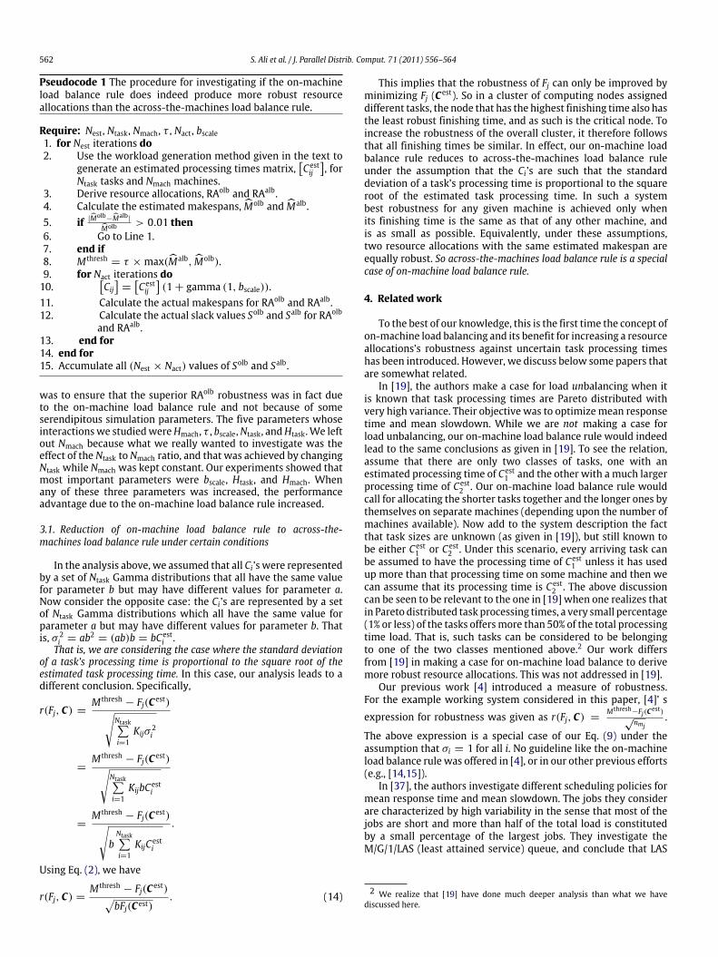
where 0(·) is the Gamma function. Fig. 3 shows how the relativechanges in a and b affect the Gamma probability density function.

From the properties of Gamma distribution, the distributionmean is ab and variance is ab2. Given that we have already fixedthe mean at Cest

i , fixing one of a or b would completely definethe Gamma distribution that, we assume, will characterize theactual task processing times, Ci’s. We will consider both cases,i.e., invariant a and invariant b.

S. Ali et al. / J. Parallel Distrib. Comput. 71 (2011) 556–564 559

Fig. 2. Relationships among Gamma, Erlang, and exponential distributions [24].

a b

Fig. 3. Figure (a) shows how the probability density function for a Gamma distribution changes when a is changed for a fixed b of 1. Figure (b) shows how the densityfunction changes when b is changed for a fixed a of 1.

As the first case, consider that all Ci’s are represented by aset of Ntask Gamma distributions that all have the same value forparameter b. Because mean = Cest

i = ab, we have that a = Cesti /b.

That is Ci = gamma(Cesti /b, b). Then, σ 2

i = ab2 = a2b2/a =

(Cesti )2/a. That is, we are considering the case where the standard

deviation of a task’s processing time is proportional to the estimatedtask processing time. Given that, Eq. (9) can be further reduced asfollows.

r(Fj, C) =M thresh

− Fj(C est)Ntask∑i=1

Kijσ2i

(10)

=M thresh

− Fj(C est)Ntask∑i=1

Kij(Cest

i )2

a

=√aM thresh

− Fj(C est)Ntask∑i=1

Kij(Cesti )2

. (11)

Now let us consider two computing nodes that have differenttasks allocated to them but still have the same estimated finishingtime (for example, computing nodes 4 and 3 in resource allocations(a) and (b) in Fig. 1). Both of these nodes have the largest estimatedfinishing time among the five computing nodes in the system, andtheir actual finishing times are probablymost likely to go above thedeadline of M thresh when the actual task processing times overruntheir estimated values. For these two machines, the numerator inEq. (11) is the same. Denote by nmj the number of applicationsallocated to mj. A little analysis (please see Appendix) shows thatthe smallest value of the denominator

∑Ntaski=1 Kij(Cest

i )2, subjectto the constraints that

∑Ntaski=1 KijCest

i = Fj(C est), occurs when

Cesti =

Fj(Cest)

nmjfor all applicationsmapped onmj. That is, the distance

between Fj(C est), the estimated finishing time of machine mj and thedeadline M thresh is the largest when all tasks mapped on mj are thesame size.

This result gives the mathematical justification for the firstspecial case of our proposed on-machine load balance rule thatwe stated earlier in Section 1. However, there is more that we canlearn from Eq. (11). Specifically, we will use it to justify the secondspecial case of the on-machine load balance rule.

As an illustration of the second special case of the on-machineload balance rule, consider two computing nodes mj and mk suchthat both have the same estimated finishing time of 100 units.There are 5 tasksmapped onmj, eachwith an estimated processingtime of 20 units. There are 4 tasks on mk, each with an estimatedprocessing time of 25 units. The second special case of the on-machine load balance rule predicts that mj’s actual finishing timeis less likely to violate the deadline.

Nowwe give amathematical justification for the second specialcase of the on-machine load balance rule. Continuing from Eq. (11),

r(Fj, C) =√a

M thresh− Fj(C est)

Ntask∑i=1

Kij

Fj(Cest)

nmj

2=

√aM thresh

− Fj(C est)

Fj(Cest)

nmj

Ntask∑i=1

Kij

.

Because∑Ntask

i=1 Kij is really just the number of applications assignedto machinemj (i.e., nmj ),

r(Fj, C) =√aM thresh

− Fj(C est)

Fj(Cest)

nmj

√nmj

=√aM thresh

− Fj(C est)

Fj(C est)

nmj

=

√aM thresh

− Fj(C est)

Fj(C est)

nmj . (12)

Eq. (12) directly gives the mathematical justification for thesecond special case of the on-machine load balance rule. The

560 S. Ali et al. / J. Parallel Distrib. Comput. 71 (2011) 556–564

equation shows that the robustness of a machine’s finishing timewhen all tasks on that machine are equally sized is directlyproportional to the number of tasks mapped on that machine. Itfollows thatwhen all tasks are infinitesimally small, the robustnessis infinite.

If our analysis is correct, then the use of on-machine loadbalance rule in resource allocation algorithms and heuristicsshould produce more robust resource allocations. That is, underthe conditions of actual processing times, the actual makespan ofthese resource allocations should be more likely to be below thethreshold ofM thresh. We show this precisely in Section 3.

3. Validating the on-machine load balance rule

Our proposed on-machine load balance rule is motivated by themathematical justification given in Section 2. However, we needto verify that when actual task processing times are substitutedfor the estimated ones, a resource allocation derived using theon-machine load balance rule will indeed perform better thananother resource allocation derived using the across-the-machinesload balance rule with minimization of the estimated makespanas the primary performance measure. To that end, we tested therobustness of a given resource allocation by subjecting it to severalinstances of simulated actual processing times and observing if theactual makespanM violated the makespan constraintM thresh.

We choose an independent task allocation system for ourvalidation experiments. The applications that arrive for executionon the system hardware are assumed to be independent,i.e., no communications between the applications are needed.This scenario is likely to be present, for instance, when manyindependent users submit their jobs to a collection of sharedcomputational resources, e.g., a cluster or a grid. Each machineexecutes a single application at a time (i.e., nomulti-tasking), in theorder inwhich the applications are assigned. Because such systemsoften execute tasks that vary widely in their computationalresource requirements, we will parameterize our validationexperiments with a measure of task heterogeneity. Similarly,since such systems have computing nodes that might varywidely in their computational capability, we will parameterize ourvalidation experiments with a measure of machine heterogeneity.

We now define some terms to help explain our validationprocedure. Let RAolb be a resource allocation derived using the on-machine load balance rule, with minimization of the estimatedmakespan as the primary performance measure. The abbreviation‘‘RA’’ stands for resource allocation. Let RAalb be another resourceallocation derived using the across-the-machines load balancerule, with minimization of the estimatedmakespan as the primaryperformance measure. Let Molb be the estimated makespan forRAolb, and Malb be the estimated makespan for RAalb. Similarly, letMolb and Malb be the actual makespan values for RAolb and RAalb,respectively. Let τ > 1 be a real number used to quantify thedeadline M thresh. Specifically, let M thresh

= τ × max(Malb,Molb).Define Solb as the difference between the pre-declared upperthreshold for makespan and the actual makespan, i.e., Solb =

M thresh− Molb. Similarly, Salb = M thresh

− Malb.The process given in Pseudocode 1 describes what constitutes

one experiment. The outer loop (Lines 1–14) of a validationexperiment is repeated Nest times. In each one of these Nestiterations, a new

Cestij

matrix is generated using the workload

generation method given later in the text, and the resourceallocations RAolb and RAalb are derived using the on-machineload balance rule and across-the-machines load balance rulerespectively.1 For each such pair of allocations, we generated Nact

1 In this paper, a genetic algorithm was used to find RAalb and RAolb in Line 3,albeit with appropriately modified fitness functions for each resource allocation.

Fig. 4. The plots of Pareto distribution’s density function for k = 1, 2, and 3. As kapproaches ∞, the density function approaches Dirac’s delta function δ(x − xmin).

realizations of the actual processing times in the inner loop (Lines9–13). For each iteration of this inner loop, an actual processingtimematrixwas generated by adding a Gamma distributed ‘‘noise’’to the

Cestij

matrix entries. Specifically, for a scale factor, bscale,

Cij

=Cestij

(1 + gamma(1, bscale)). The actual processing times

were then used to determine the values of Solb and Salb.The values of Nest and Nact were chosen to be 50 and 300,

respectively, giving a total of 15,000 trials. For a given iterationof the outer loop, the inner loop was not taken if the differencebetween the estimated makespans of RAolb and RAalb was morethan 1%. Thiswas done to ensure that only resource allocations thathad equally good makespans were compared for robustness. Onlya few trials were lost because of this, and we report that with eachexperiment.

We assumed highly heterogeneous tasks and machines. Fora given task, ai, its processing times on different machine weregenerated to be heterogeneous, with themeasure of heterogeneitybeing the coefficient of variation, Htask of the generated times. Fora given machine, mi, its processing times for different tasks weregenerated to be heterogeneous, with themeasure of heterogeneitybeing the coefficient of variation,Hmach of the generated times. Theexperiments were performed for two source distributions for theestimated task processing times: Pareto and Gamma. The Gammadistribution was used because of its generality and the Paretodistribution was used because many researchers have shown thattask processing times are often Pareto distributed or otherwisehave high variability (e.g., [20,38]).

A Pareto distribution with shape parameter k and locationparameter xmin has the following probability distribution

f (x) = kxkmin

xk+1. (13)

Note that xmin is the minimum value of x. Fig. 4 shows plotsof Pareto distribution density function for three values of k. Ask approaches ∞, the density function approaches Dirac’s deltafunction δ(x − xmin).Workload generation method: The following procedure produces aCestij

matrix given Htask and Hmach as the desired coefficients of

variations for the rows and columns, respectively, of theCestij

matrix. The values in an

Cestij

matrix could be Pareto or Gamma

distributed. The parameter l signifies the smallest value in the caseof a Pareto distributed

Cestij

. For a Gamma distributed

Cestij

, it

equals the desired mean of theCestij

matrix. It is assumed that

Htask ≥ Hmach. A slightly different procedure is employed whenHtask ≤ Hmach.

S. Ali et al. / J. Parallel Distrib. Comput. 71 (2011) 556–564 561

1. Htask and Hmach are the desired coefficients of variations for therows and columns of the

Cestij

matrix.

Htask and Hmach are the actual coefficients of variations for therows and columns of the

Cestij

matrix that is produced in this

procedure.2. Flag = 0 /* This flag is set to 1 during the procedure when

the desired and actual values of the coefficients of variationsfor the rows and columns of the

Cestij

matrix are close within a

tolerance of 10%. */3. while Flag is 0 do4. if the desired distribution is Pareto then5. Generate a vector Vm by sampling pareto(Htask, l) for

Ntask times.6. for i = 1 to Ntask do7. Generate the i-th column of the

Cestij

matrix by

samplingpareto(Hmach, Vm(i)) for Nmach times.

8. end for9. else if the desired distribution is Gamma then10. Generate a vector Vm by sampling gamma(1/H2

task,

H2taskl) for Ntasktimes.

11. for i = 1 to Ntask do12. Generate the i-th column of the

Cestij

matrix by

sampling gamma(1/H2mach,H

2machVm(i)) for Nmach

times.13. end for14. end if15. Calculate Hmach, the actual mean of coefficients of

variation of the columns ofCestij

16. Calculate Htask, the actual mean of coefficients of variation

of the rows ofCestij

17. if |Htask−Htask|

Htask< 0.1 and |Hmach−Hmach|

Hmach< 0.1 then

18. Flag = 119. else20. Flag = 021. end if22. end while

We conducted a number of experiments, varying differentexperiment parameters. Fig. 5 shows the results for one set ofparameters for an experiment where

Cestij

was generated by

sampling a Gamma distribution. We first ‘‘normalized’’ Solb andSalb with their respective estimated makespan values, and thenplotted the CDFs for the normalized slack values, i.e., for SolbMolb

and SalbMalb . This was done to make the x-axis more meaningfulacross different experiments. From Fig. 5, one can see that forall values of x, Prob

SolbMolb ≤ x

≤ Prob

SalbMalb ≤ x

, i.e., the

probability that the normalized slack is no more than x issmaller (i.e., better) for resource allocations derived using theon-machine load balance rule than for those derived using theacross-the-machines load balance rule. In particular note thatProb

SalbMalb ≤ 0

− Prob

SolbMolb ≤ 0

= 0.132. That is, the

number of RAalb allocations that violated the makespan limit was13.2% more than the number of RAolb allocations that violatedthe makespan limit. This is very significant, especially since theestimated makespan of RAolb was no more than 1% different fromthe estimated makespan of RAalb.

Fig. 6 show the results for an experiment whereCestij

was

generated by sampling a Pareto distribution. One can see that for

Fig. 5. This figure shows that the probability of the actual makespan violating thedeadline is 13.2% smaller for the resource allocations produced by following theon-machine load balance rule. The cumulative distribution function was plottedfor 12,300 samples of the ratio of actual slack to the estimated makespan forRAolb and RAalb . Experiment parameters were set so that Ntask = 100,Nmach =

10,Htask = 3.73,Hmach = 1.63, bscale = 2, and τ = 4. The estimated task timeswere generated by sampling a Gamma distribution using the method given in theworkload generation method given before.

Fig. 6. This figure shows that the probability of the actual makespan violating thedeadline is 14.4% smaller for the resource allocations produced by following theon-machine load balance rule. The cumulative distribution function was plotted for14,700 samples of the ratio of actual slack to the estimated makespan for RAolb andRAalb . Experiment parameters were set so that Ntask = 100,Nmach = 10,Htask =

1.86,Hmach = 0.81, bscale = 2, and τ = 4. The estimated task times weregenerated by sampling a Pareto distribution using themethod given in theworkloadgeneration method given before.

most values of x, Prob

SolbMolb ≤ x

≤ Prob

SalbMalb ≤ x, i.e., the

probability that the normalized slack is no more than x issmaller (i.e., better) for resource allocations derived using theon-machine load balance rule than for those derived using theacross-the-machines load balance rule. In particular note thatProb

SalbMalb ≤ 0

− Prob

SolbMolb ≤ 0

= 0.144. That is, the number

of RAalb allocations that violated the makespan limit was 14.4%more than the number of RAolb allocations that violated themakespan limit. Once again, this is very significant, especially sincethe estimated makespan of RAolb was no more than 1% differentfrom the estimated makespan of RAalb.

We conducted a 25−1 fractional factorial experiment for fivedifferent parameter combinations to determine the dependenceof results on the parameters used in the experiment. Our intent

562 S. Ali et al. / J. Parallel Distrib. Comput. 71 (2011) 556–564

Pseudocode 1 The procedure for investigating if the on-machineload balance rule does indeed produce more robust resourceallocations than the across-the-machines load balance rule.

Require: Nest, Ntask, Nmach, τ , Nact, bscale1. for Nest iterations do2. Use the workload generation method given in the text to

generate an estimated processing times matrix,Cestij

, for

Ntask tasks and Nmach machines.3. Derive resource allocations, RAolb and RAalb.4. Calculate the estimated makespans, Molb and Malb.5. if |Molb

−Malb|Molb > 0.01 then

6. Go to Line 1.7. end if8. M thresh

= τ × max(Malb,Molb).9. for Nact iterations do10.

Cij

=Cestij

(1 + gamma (1, bscale)).

11. Calculate the actual makespans for RAolb and RAalb.12. Calculate the actual slack values Solb and Salb for RAolb

and RAalb.13. end for14. end for15. Accumulate all (Nest × Nact) values of Solb and Salb.

was to ensure that the superior RAolb robustness was in fact dueto the on-machine load balance rule and not because of someserendipitous simulation parameters. The five parameters whoseinteractionswe studiedwereHmach, τ , bscale,Ntask, andHtask.We leftout Nmach because what we really wanted to investigate was theeffect of the Ntask to Nmach ratio, and that was achieved by changingNtask while Nmach was kept constant. Our experiments showed thatmost important parameters were bscale, Htask, and Hmach. Whenany of these three parameters was increased, the performanceadvantage due to the on-machine load balance rule increased.

3.1. Reduction of on-machine load balance rule to across-the-machines load balance rule under certain conditions

In the analysis above, we assumed that all Ci’s were representedby a set of Ntask Gamma distributions that all have the same valuefor parameter b but may have different values for parameter a.Now consider the opposite case: the Ci’s are represented by a setof Ntask Gamma distributions which all have the same value forparameter a but may have different values for parameter b. Thatis, σ 2

i = ab2 = (ab)b = bCesti .

That is, we are considering the case where the standard deviationof a task’s processing time is proportional to the square root of theestimated task processing time. In this case, our analysis leads to adifferent conclusion. Specifically,

r(Fj, C) =M thresh

− Fj(C est)Ntask∑i=1

Kijσ2i

=M thresh

− Fj(C est)Ntask∑i=1

KijbCesti

=M thresh

− Fj(C est)b

Ntask∑i=1

KijCesti

.

Using Eq. (2), we have

r(Fj, C) =M thresh

− Fj(C est)bFj(C est)

. (14)

This implies that the robustness of Fj can only be improved byminimizing Fj (C est). So in a cluster of computing nodes assigneddifferent tasks, the node that has the highest finishing time also hasthe least robust finishing time, and as such is the critical node. Toincrease the robustness of the overall cluster, it therefore followsthat all finishing times be similar. In effect, our on-machine loadbalance rule reduces to across-the-machines load balance ruleunder the assumption that the Ci’s are such that the standarddeviation of a task’s processing time is proportional to the squareroot of the estimated task processing time. In such a systembest robustness for any given machine is achieved only whenits finishing time is the same as that of any other machine, andis as small as possible. Equivalently, under these assumptions,two resource allocations with the same estimated makespan areequally robust. So across-the-machines load balance rule is a specialcase of on-machine load balance rule.

4. Related work

To the best of our knowledge, this is the first time the concept ofon-machine load balancing and its benefit for increasing a resourceallocations’s robustness against uncertain task processing timeshas been introduced. However, we discuss below some papers thatare somewhat related.

In [19], the authors make a case for load unbalancing when itis known that task processing times are Pareto distributed withvery high variance. Their objective was to optimizemean responsetime and mean slowdown. While we are not making a case forload unbalancing, our on-machine load balance rule would indeedlead to the same conclusions as given in [19]. To see the relation,assume that there are only two classes of tasks, one with anestimated processing time of Cest

1 and the other with a much largerprocessing time of Cest

2 . Our on-machine load balance rule wouldcall for allocating the shorter tasks together and the longer ones bythemselves on separate machines (depending upon the number ofmachines available). Now add to the system description the factthat task sizes are unknown (as given in [19]), but still known tobe either Cest

1 or Cest2 . Under this scenario, every arriving task can

be assumed to have the processing time of Cest1 unless it has used

up more than that processing time on some machine and then wecan assume that its processing time is Cest

2 . The above discussioncan be seen to be relevant to the one in [19] when one realizes thatin Pareto distributed task processing times, a very small percentage(1% or less) of the tasks offersmore than 50% of the total processingtime load. That is, such tasks can be considered to be belongingto one of the two classes mentioned above.2 Our work differsfrom [19] in making a case for on-machine load balance to derivemore robust resource allocations. This was not addressed in [19].

Our previous work [4] introduced a measure of robustness.For the example working system considered in this paper, [4]’ s

expression for robustness was given as r(Fj, C) =Mthresh

−Fj(Cest)√

nmj.

The above expression is a special case of our Eq. (9) under theassumption that σi = 1 for all i. No guideline like the on-machineload balance rule was offered in [4], or in our other previous efforts(e.g., [14,15]).

In [37], the authors investigate different scheduling policies formean response time and mean slowdown. The jobs they considerare characterized by high variability in the sense that most of thejobs are short and more than half of the total load is constitutedby a small percentage of the largest jobs. They investigate theM/G/1/LAS (least attained service) queue, and conclude that LAS

2 We realize that [19] have done much deeper analysis than what we havediscussed here.

S. Ali et al. / J. Parallel Distrib. Comput. 71 (2011) 556–564 563

favors short jobs with a negligible penalty to the few largestjobs. Our work is different because we have used the variabilityinformation to mathematically justify and statistically prove theon-machine load balance rule that can be used to derive resourceallocations that are robust against uncertain task processing times.

In [50], the authors propose a conservative scheduling pol-icy that uses information about expected future variance inresource capabilities to produce more efficient data mappingdecisions. They consider heterogeneous and dynamic environ-ments, where task processing time is variable. Their results showthat conservative scheduling can produce execution times that areboth significantly faster and less variable than other techniques.Essentially, the approach in [50] assigns less work to less reliable(or higher variance) resources. Once again, our work differs in itsgenerality.

Probabilistic QoS guarantees for supercomputing systems areproposed in [34]. The proposed approach enables the system andusers to negotiate a mutually desirable risk strategy, and makesprobabilistic guarantees on quality of service such that ‘‘job j can becompleted by deadline d with probability p’’. A metric for qualityof service is presented in this paper, and the scheduler tries tomaximize the quality of service using this metric.

In [11], the author studies diffusion schemes for dynamicload balancing on message passing multiprocessor networks, andprovides conditions for and rates of convergence to a uniformworkdistribution for arbitrary topologies. The author further showsthat for a hypercube topology, an approach called dimensionexchange provides better convergence compared to diffusion. Thisessentially calls for the equal sharing of workload between eachadjacent pair of processors within the hypercube. The researchpresented in [11] has a different focus than our work. Our resultsstrive for robustness in the face of uncertainties in task processingtimes while [11] focuses on analytically sound protocols for loadbalancing.

A semi-distributed strategy for task scheduling and load bal-ancing in large distributed systems is proposed in [2]. The inter-connection network is partitioned into independent symmetricregions (spheres) containing nodes centered at some control points(schedulers). Load is first balanced among the various spheres inthe network, and then load balancing is performed within each ofthe respective spheres. The approach presented in this paper doesnot preclude our work, since we have defined a general rule formaking resource allocations more robust in situations where taskprocessing times are volatile. Indeed, our results could effectivelybe incorporated into this and similar load balancing algorithms toimprove robustness against task processing time uncertainties.

In [20], the authors propose a functional form that fitsthe distribution of lifetimes for Unix processes. They use thisformulation to derive a policy for preemptive migration, andshow that the performance benefits of preemptive migration aresignificantly higher than those of non-preemptive migration. Asin [11,20] it has a different focus than ours, specifically loadbalancing techniques.

A number of robustness measures have been previously pro-posed e.g., [7,12,16,18,21,26,25,29,42,44]; they were all developedwith a specific system in mind, and do not attempt to capture thegeneral applicability of ourmethodology. Please see [4] for detaileddescriptions of the above research efforts.

Unlike these previous efforts, our work is based on a generalmathematical formulation of a robustness metric that can be ap-plied to a variety of parallel and distributed systems by followingthe general theoretical procedure summarized in this paper. Wealso notemany related articles from the field of stochastic schedul-ing (e.g., [1,8–10,17,23,22,27,31,35,36,40,39,41,43,46,47,49]). Asurvey can be found here [33]. The focus of the papers cited abovewas somewhat different, and most of them made several assump-tions (e.g., single server, identical machines, exponentially dis-tributed processing times) that our approach does not require.

5. Conclusions

This paper introduces a new principle called the on-machineload balance rule. The on-machine load balance rule states that fortwo computing nodes that have the same estimated finishing time,and the same deadline before which the nodes must process theirload, the node that has a larger number of tasks and more equallysized tasks mapped on it is less likely to violate the deadline.

We show that, under some very liberal assumptions, the on-machine load balance rule leads to resource allocations that arebetter in tolerating uncertainties in the processing times of thetasks allocated to the resources when compared to other resourceallocations that are derived using the conventional ‘‘across themachines’’ load balancing rule. Specifically, we show in this paperthat the resource allocations derived using the on-machine loadbalance rule are less likely to violate a deadline placed on theoverall completion time of the set of tasks than other resourceallocations that have not followed the on-machine load balancerule, even if they still have the same estimated makespan.

The on-machine load balance rule calls for the resourceallocation algorithms to allocate similarly sized tasks on amachine. We give a mathematical justification for the on-machineload balance rule requiring only liberal assumptions about taskprocessing times.We then validatewith extensive simulations thatthe resource allocations derived using on-machine load balancerule are indeed more tolerant of uncertain task processing times.

Appendix

Here we prove that the smallest value of the function

f (C est) =

Ntask−i=1

Kij(Cesti )2 (15)

subject to the constraint∑Ntask

i=1 KijCesti = Fj(C est) occurs when

Cesti =

Fj(Cest)

nmjfor all applications mapped onmj. Let

g(C est) =

Ntask−i=1

KijCesti − Fj(C est) = 0. (16)

Let C⋆ be the optimal point. Using the Lagrange multiplierapproach, ∇f (C est) + λ∇g(C est) = 0. That is, for i = 1 · · ·Ntask,

∂ f∂Cest

i+ λ

∂g∂Cest

i= 0

or

2C⋆i + λ = 0

C⋆i = −

λ

2. (17)

Using Eq. (17) in Eq. (16), we get

−λnmj

2= Fj(C est)

λ =−2Fj(C est)

nmj

. (18)

Using Eq. (18) in Eq. (17)

C⋆i =

Fj(C est)

nmj

. (19)

This completes the proof.

564 S. Ali et al. / J. Parallel Distrib. Comput. 71 (2011) 556–564

References

[1] A. Agrawala, E. Coffman Jr., M. Garey, S. Tripathi, A stochastic optimizationalgorithm minimizing expected flow times on uniform processors, IEEETransactions on Computers 33 (1984) 351–356.

[2] I. Ahmad, A. Ghafoor, Semi-distributed load balancing for massively parallelmulticomputer systems, IEEE Transactions on Software Engineering 17 (10)(1991) 987–1004.

[3] S. Ali, T.D. Braun, H.J. Siegel, N. Beck, L. Bölöni, M. Maheswaran, A.I. Reuther,J.P. Robertson,M.D. Theys, B. Yao, Characterizing resource allocation heuristicsfor heterogeneous computing systems, in: A.R. Hurson (Ed.), Parallel,Distributed, and Pervasive Computing, in: Advances in Computers, vol. 63,Elsevier Academic Press, San Diego, CA, 2005, pp. 91–128.

[4] S. Ali, A.A. Maciejewski, H.J. Siegel, J.-K. Kim, Measuring the robustness of aresource allocation, IEEE Transactions on Parallel and Distributed Systems 15(7) (2004) 630–641.

[5] I. Banicescu, V. Velusamy, Performance of scheduling scientific applicationswith adaptive weighted factoring, in: 10th IEEE Heterogeneous ComputingWorkshop, HCW 2001, in the Proceedings of the 15th International Paralleland Distributed Processing Symposium, IPDPS 2001, April 2001.

[6] H. Barada, S.M. Sait, N. Baig, Task matching and scheduling in heterogeneoussystems using simulated evolution, in: 10th IEEE Heterogeneous ComputingWorkshop, HCW 2001, in the Proceedings of the 15th International Paralleland Distributed Processing Symposium, IPDPS 2001, April 2001.

[7] L. Bölöni, D.C.Marinescu, On the robustness ofmetaprogram schedules, in: 8thIEEE Heterogeneous ComputingWorkshop, HCW’99, April 1999, pp. 146–155.

[8] J. Bruno, P. Downey, G. Fredrickson, Sequencing taskswith exponential servicetimes tominimize the expected flow time ormakespan, Journal of the ACM 28(1981) 100–113.

[9] C.-S. Chang, R. Nelson, M. Pinedo, Scheduling two classes of exponential jobson parallel processors: structural results and worst case analysis, Journal ofApplied Probability (1991).

[10] C.-S. Chang, R. Righter, The optimality of LEPT in parallel machine scheduling,Journal of Applied Probability 31 (1994) 788–796.

[11] G. Cybenko, Dynamic load balancing for distributed memory multiprocessors,Journal of Parallel and Distributed Computing 7 (2) (1989) 279–301.

[12] R.L. Daniels, J.E. Carrillo, β-robust scheduling for single-machine systemswithuncertain processing times, IIE Transactions 29 (11) (1997) 977–985.

[13] M.M. Eshaghian (Ed.), Heterogeneous Computing, Artech House, Norwood,MA, 1996.

[14] B. Eslamnour, S. Ali, A probabilistic approach to measuring robustness incomputing systems, in: 21st International Parallel and Distributed ProcessingSymposium, IPDPS 2007, 2007.

[15] B. Eslamnour, S. Ali, Measuring robustness of computing systems, SimulationModelling Practice and Theory (2009) Available at:http://dx.doi.org/10.1016/j.simpat.2009.06.004.

[16] S. Ghosh, Guaranteeing fault tolerance through scheduling in real-timesystems, Ph.D. Thesis, Faculty of Arts and Sciences, Univ. of Pittsburgh, 1996.

[17] A. Goel, P. Indyk, Stochastic load balancing and related problems, in: 40thAnnual Symposium on Foundations of Computer Science, 1999, pp. 579–586.

[18] S.D. Gribble, Robustness in complex systems, in: 8th Workshop on Hot Topicsin Operating Systems, HotOS-VIII, May 2001, pp. 21–26.

[19] M. Harchol-Balter, Task assignment with unknown duration, Journal of theACM 49 (2) (2002) 260–288.

[20] M. Harchol-Balter, A.B. Downey, Exploiting process lifetime distributions fordynamic load balancing, ACMTransactions onComputer Systems15 (3) (1997)253–285.

[21] D.E. Hastings, A.L. Weigel, M.A. Walton, Incorporating uncertainty intoconceptual design of space system architectures, in: ESD Internal Symposium,Working Paper Series, ESD-WP-2003-01.01, May 2002.

[22] A. Hordijk, G. Koole, On the assignment of customers to parallel queues,Probability in the Engineering and Informational Sciences 6 (1992) 495–512.

[23] C. Huang, G. Weiss, Preemptive scheduling of stochastic jobs with a two stageprocessing time distribution, Probability in the Engineering and InformationalSciences 6 (1992).

[24] R. Jain, The Art of Computer Systems Performance Analysis, JohnWiley & Sons,Inc., New York, NY, 1991.

[25] E. Jen, Stable or robust? What is the difference? Santa Fe Institute WorkingPaper No. 02-12-069, 2002.

[26] M. Jensen, Improving robustness and flexibility of tardiness and total flow timejob shops using robustness measures, Journal of Applied Soft Computing 1 (1)(2001) 35–52.

[27] T. Kämpke, Optimal scheduling of jobs with exponential service times onidentical parallel processors, Operations Research 37 (1989) 126–133.

[28] A. Khokhar, V.K. Prasanna, M. Shaaban, C.L. Wang, Heterogeneous computing:challenges and opportunities, IEEE Computer 26 (6) (1993) 18–27.

[29] V.J. Leon, S.D. Wu, R.H. Storer, Robustness measures and robust scheduling forjob shops, IEE Transactions 26 (5) (1994) 32–43.

[30] M.Maheswaran, S. Ali, H.J. Siegel, D. Hensgen, R.F. Freund, Dynamicmapping ofa class of independent tasks onto heterogeneous computing systems, Journalof Parallel and Distributed Computing 59 (2) (1999) 107–131.

[31] G. Malewicz, Parallel scheduling of complex DAGs under uncertainty, in: 17thAnnual ACMSymposiumonParallelism inAlgorithms andArchitectures, 2005,pp. 66–75.

[32] Z. Michalewicz, D.B. Fogel, How to Solve It: Modern Heuristics, Springer-Verlag, New York, NY, 2000.

[33] J. Nino-Mora, Stochastic scheduling, in: C.A. Floudas, P.M. Pardalos (Eds.),Encyclopedia of Optimization, Kluwer, 2001, pp. 367–372.

[34] A.J. Oliner, L. Rudolph, R.K. Sahoo, J.E. Moreira, M. Gupta, ProbabilisticQoS guarantees for supercomputing systems, in: The 2005 InternationalConference on Dependable Systems and Networks, DSN 2005, June–July 2005,pp. 634–643.

[35] M. Pinedo, Minimizing the expected makespan in stochastic flow shops,Operations Research 30 (1982) 148–162.

[36] M. Pinedo, G. Weiss, The ‘‘largest variance first’’ policy in some stochasticscheduling problems, Operations Research 35 (1987) 884–891.

[37] I.A. Rai, G. Urvoy-Keller, E.W. Biersack, Analysis of LAS scheduling for job sizedistributions with high variance, in: The 2003 ACM SIGMETRICS InternationalConference on Measurement and Modeling of Computer Systems, 2003,pp. 218–228.

[38] S. Ray, R. Ungrangsi, F.D. Pellegrinin, A. Trachtenberg, D. Starobinski, Robustlocation detection in emergency sensor networks, in: The 22nd Annual JointConference of the IEEE Computer and Communications Societies, INFOCOM2003, April 2003.

[39] R. Righter, S. Xu, Scheduling jobs on heterogeneous processors, Annals ofOperations Research 28 (1991) 587–602.

[40] R. Righter, S. Xu, Scheduling jobs on nonidentical IFR processors to minimizegeneral cost functions, Advances in Applied Probability 23 (1991) 909–924.

[41] J.M. Schopf, F. Berman, Stochastic scheduling, IEEE Supercomputing (1999).[42] M. Sevaux, K. Sörensen, Genetic algorithm for robust schedules, in: 8th

International Workshop on Project Management and Scheduling, PMS 2002,April 2002, pp. 330–333.

[43] M. Skutella, M. Uetz, Scheduling precedence-constrained jobs with stochasticprocessing times on parallel machines, in: 12th Annual ACM–SIAM Sympo-sium on Discrete Algorithms, SODA 2001, 2001, pp. 589–590.

[44] Y.N. Sotskov, V.S. Tanaev, F. Werner, Stability radius of an optimal schedule:a survey and recent developments, in: G. Yu (Ed.), Industrial Applications ofCombinatorial Optimization, Kluwer Academic Publishers, Norwell, MA, 1998,pp. 72–108.

[45] M. Stastny, Mahalanobis distance, 2001.http://www.wu-wien.ac.at/usr/h99c/h9951826/distance.pdf.

[46] G. Weiss, M. Pinedo, Scheduling tasks with exponential service times on non-identical processors to minimize various cost functions, Journal of AppliedProbability 17 (1980) 187–202.

[47] W. Whitt, Deciding which queue to join: some counter examples, OperationsResearch 34 (1986) 55–62.

[48] M.-Y. Wu, W. Shu, H. Zhang, Segmented min–min: a static mappingalgorithm for meta-tasks on heterogeneous computing systems, in: 9th IEEEHeterogeneous Computing Workshop, HCW 2000, May 2000, pp. 375–385.

[49] S. Xu, Stochastically minimizing total delay of jobs subject to randomdeadlines, Probability in the Engineering and Informational Sciences 5 (1991)333–348.

[50] L. Yang, J.M. Schopf, I. Foster, Conservative scheduling: using predictedvariance to improve scheduling decisions in dynamic environments, in: The2003 ACM/IEEE Conference on Supercomputing, 2003, pp. 1–16.

Shoukat Ali is a research scientist with IBM. He worksat Exascale Stream Computing Collaboratory, a part ofIBM Research’s Smarter City Technology Center in Dublin,Ireland. He was previously in platform validation atIntel, which he joined in April 2007. Before that he wasan assistant professor in the Electrical and ComputerEngineering Department at the University of Missouri-Rolla. Dr. Ali received his B.S. degree in ElectricalEngineering from the University of Engineering andTechnology, Lahore, Pakistan. He joined PurdueUniversity,West Lafayette for his graduate studies, and received

his M.S. and Ph.D. in Electrical and Computer Engineering in August 1999 andAugust 2003, respectively. He has 32 publications in the areas of algorithms, logicpartitioning, performance analysis, and robust resource allocation.

Behdis Eslamnour received the M.S. degree in electrical engineering in 2000 fromtheDepartment of Electrical Engineering at the Amirkabir University of Technology,Tehran, Iran. She received the B.S. degree in electrical engineering in 1996 fromthe Sharif University of Technology, Tehran, Iran. She is a graduate student in theDepartment of Electrical and Computer Engineering at the Missouri University ofScience and Technology, Rolla, where she is currently a research assistant. Herresearch interests include networks, heterogeneous distributed computing andresource management. She is a student member of the IEEE.

Zehra Shah received her B.S. and M.S. degrees in Com-puter Science from the Lahore University of ManagementSciences, Lahore, Pakistan in 2003 and 2005 respectively.Later, she worked as a research assistant in the computervision and pattern classification lab at the Lahore Univer-sity of Management Sciences in the machine learning anddata mining group. Her research interests include algo-rithms, performance analysis, machine learning, and pat-tern classification.