A Case for IncludingAtmospheric ThermodynamicVariables in Wind TurbineFatigue Loading ParameterIdentification

July 1999 • NREL/CP-500-26829

Neil D. KelleyNational Wind Technology Center

Second Symposium onWind Conditions for Wind Turbine DesignIEA Annex XIRoskilde, DenmarkApril 12–13, 1999

National Renewable Energy Laboratory1617 Cole BoulevardGolden, Colorado 80401-3393

NREL is a U.S. Department of Energy LaboratoryOperated by Midwest Research Institute •••• Battelle •••• Bechtel

Contract No. DE-AC36-98-GO10337

NOTICE

This report was prepared as an account of work sponsored by an agency of the United Statesgovernment. Neither the United States government nor any agency thereof, nor any of their employees,makes any warranty, express or implied, or assumes any legal liability or responsibility for the accuracy,completeness, or usefulness of any information, apparatus, product, or process disclosed, or representsthat its use would not infringe privately owned rights. Reference herein to any specific commercialproduct, process, or service by trade name, trademark, manufacturer, or otherwise does not necessarilyconstitute or imply its endorsement, recommendation, or favoring by the United States government or anyagency thereof. The views and opinions of authors expressed herein do not necessarily state or reflectthose of the United States government or any agency thereof.

Available to DOE and DOE contractors from:Office of Scientific and Technical Information (OSTI)P.O. Box 62Oak Ridge, TN 37831

Prices available by calling 423-576-8401

Available to the public from:National Technical Information Service (NTIS)U.S. Department of Commerce5285 Port Royal RoadSpringfield, VA 22161703-605-6000 or 800-553-6847orDOE Information Bridgehttp://www.doe.gov/bridge/home.html

Printed on paper containing at least 50% wastepaper, including 20% postconsumer waste

1

IEA Annex XI2nd Symposium, Wind Conditions for Turbine DesignRisø National LaboratoryRoskilde, DK , 12-13 April 1999

A CASE FOR INCLUDING ATMOSPHERICTHERMODYNAMIC VARIABLES INWIND TURBINE FATIGUE LOADINGPARAMETER IDENTIFICATION

N.D. KelleyNational Wind Technology CenterNational Renewable Energy LaboratoryGolden, Colorado U.S.A.

ABSTRACT

This paper makes the case for establishing efficient predictor variables for atmospheric thermodynamics

that can be used to statistically correlate the fatigue accumulation seen on wind turbines. Recently, two

approaches to this issue have been reported. One uses multiple linear-regression analysis to establish the

relative causality between a number of predictors related to the turbulent inflow and turbine loads. The

other approach, using many of the same predictors, applies the technique of principal component analysis.

An examination of the ensemble of predictor variables revealed that they were all kinematic in nature;

i.e., they were only related to the description of the velocity field. Boundary-layer turbulence dynamics

depends upon a description of the thermal field and its interaction with the velocity distribution. We used

a series of measurements taken within a multi-row wind farm to demonstrate the need to include

atmospheric thermodynamic variables as well as velocity-related ones in the search for efficient

turbulence loading predictors in various turbine-operating environments. Our results show that a

combination of vertical stability and hub-height mean shearing stress variables meet this need over a

period of 10 minutes.

INTRODUCTION

A recent study has recently identified and modeled the dominant inflow turbulence-scaling parameters

responsible for the accumulation of fatigue in wind turbines operating in complex terrain environments.

Called MONTURB, this international, multi-laboratory effort analyzed measurements of both the inflow

turbulence and wind turbine dynamic variables for several turbines in both relatively smooth and complex

terrain sites in Greece, Denmark, Spain, and the United States (California) [1,2,3]. Using sensitivity

2

analysis, analysts concluded that the fatigue loads increased significantly with the standard deviation of

the longitudinal wind speed (σu), which was also considered as the primary fatigue driver. One part of the

MONTURB study [4], which was incorporated in [2], applied multivariate regression to analyze the

statistical response of turbine fatigue loads to a wide range of turbulence descriptors (including higher

order statistical moments). These analyses were based on data from a substantial array of turbulence and

load measurements taken for a single turbine installed at the crest of a hill in Greece. A similar study

conducted in Spain used principal component analysis to examine the effect of several turbulence

descriptor variables on fatigue-load factors [5].

The turbulence descriptors used as explanatory or predictor variables in [2, 4] included the following

• Mean wind speed (U)

• Power law wind-shear exponent (α)

• Inclination angle between the wind vector and the horizontal (ψ)

• Standard deviations of the longitudinal, lateral, and vertical wind components (σu, σv, and σw)

• Longitudinal, lateral, and vertical turbulence length scales (Lu, Lv, and Lw)

• Skewness of U [σ3(U)]

• Kurtosis of U [σ4(U)]

• Davenport decay factor between two elevations (Az1 and Az2)

• Ratios σv/σu and σw/σu.

The cross-correlation of the longitudinal and vertical wind components (ρuw) and the U, σu, σ3(U), σ4(U),

σv/σu, and σw/σu parameters was used by [5].

In both studies, the response variable chosen was the equivalent load parameter defined by

Equivalent Load = Leq = m

eq

mii

N

Ln1

∑

where ni is the number of cycles in the ith load range, Li is the maximum (conservative) value of each

load level in a bin, Neq is the equivalent number of constant-amplitude cycles, and m is the slope of the

material S-N curve. For these studies, record lengths of 10 minutes were used and a 1-Hz equivalent load

calculated, which set Neq to 1200 half-cycles for that period. The effect of various materials was

evaluated by applying S-N curve slopes in the range of 4 to 12. Using this definition, Leq repeated Neq

times is equivalent to the same fatigue damage contained in the measured load spectrum [2].

3

A review of the above-mentioned turbulence descriptors used as predictor variables results in the

realization that they are all kinematic; i.e., they are all related to the description of the inflow velocity

field. In 1994, we reported on the results of a similar experiment involving the 10-minute load response

of two side-by-side wind turbines deep within a multi-row wind farm in San Gorgonio Pass, California

[6]. We also applied multivariate regression and the analysis of variance (ANOVA) to assess the

sensitivity of a range of turbulence descriptors on the measured loading spectra. Our predictor variable

list, although including many of the variables listed above, also contained the following kinematic

variables and their higher moments measured at hub height:

• Mean horizontal wind speed, defined by 22H VUU +=

• Standard deviation of UH (σH)

• Turbulence intensity (σH/UH)

• Mean longitudinal, lateral, and vertical wind components aligned with the mean shear vector (U, V,

and W)

• Reynolds stress components (u'w', u'v', and v'w') where u', v', and w' are the zero-mean, fluctuating

components of U, V, and W

• Local friction velocity, defined by u* = w'u'

• Cross-correlation coefficients of u'w', u'v', and v'w' (ρu'w', ρu'v', ρv'w')

• Standard deviations of the instantaneous Reynolds stresses (σu'w', σu'v', σv'w')

• Skewness coefficients of instantaneous values of u'w', u'v', and v'w' [σ3(u'w'), σ3(u'v'), σ3(v'w')]

• Kurtosis coefficients of instantaneous values of u'w', u'v', and v'w' [σ4(u'w'), σ4(u'v'), σ4(v'w')].

In addition to the kinematic variables and their derivations listed above, we also included the following

parameters that are related to the thermodynamics of the planetary boundary layer:

• turbine-layer gradient Richardson number (Ri) stability parameter defined by

Ri = ( ) ( ) ( )���

��� ∂∂∂∂

2z/Uz/g/ θθ m

where g is the gravity acceleration, z is the height in meters, θm is the layer mean thermodynamic

potential temperature (K) given by θ(z) = T(z)[1000/p(z)]0.286 , and T(z) and p(z) are the temperature

(K) and barometric pressure (hPa), respectively at height z. The turbine layer is defined as the

4

vertical distance between the surface and the maximum elevation of the wind turbine rotor. The

over bars represent 10-minute averages.

• Hub potential temperature (θhub)

• Cross-correlation coefficient of w'θ hub' (ρw'θ')

• w'θ'' covariance or vertical temperature flux ( 'w' hubθ )

• Standard deviation, skewness, and kurtosis of 'w' hubθ .

The response variable we used for most load parameters, except edgewise bending, was the slope (β1) of

the high-loading tail or low-cycle, high-amplitude portion of the loading spectral distribution. This tail

region is a major contributor to the fatigue damage seen in materials with large S-N slopes. The loading

spectral tails are fitted with an exponential distribution pp−= M-o

1e- N ββ , where M is the peak-to-peak or

alternating load range and N is the number of cycles.

We also found that the slope β1 was most sensitive to the atmospheric stability expressed by the turbine

layer Ri and the u'w'-component of the Reynolds stress or its square root, u*. We observed that the slope

varied indirectly with u* and Ri; e.g., higher values of u* and/or Ri produced a shallower slope and higher

potential fatigue damage and vice versa. These results indicated that, at the minimum, both a kinematic

and a thermodynamic turbulence-related descriptor are necessary for a linear, multivariate regression

model that can explain a high percentage of the observed variance. Finally, we found that more than 89%

of the observed variance of the combined turbine flapwise loads could thus be explained.

A CASE STUDY WITHIN A LARGE, MULTI-ROW WIND FARM

In 1990, the National Renewable Energy Laboratory (NREL) operated two adjacent Micon 65/13 wind

turbines deep within a very large wind farm in San Gorgonio Pass, California. Both of the turbines were

identical except that one used a rotor based on the NREL 7.9m Thin Airfoil Family; the other was an

original AeroStar design. We will refer to the turbine using the NREL blades as Rotor 1 and the

AeroStar-equipped turbine as Rotor 2. A total of 397 10-minute records were taken over a wide range of

inflow conditions during late July and August, the latter half of the San Gorgonio wind season.

Inflow measurements for the turbines were taken using a near-hub-height (21-m), three-axis sonic

anemometer/thermometer and propeller-vane anemometers installed at three elevations. Temperature,

5

vertical temperature difference, and the barometric pressure were also recorded. The maximum height of

the rotors was 31 meters above ground and the turbine hubs were located at 23 meters. The two test

turbines were located downwind, with respect to the prevailing wind direction, about mid-row in Row 37

of a 41-row wind farm that included nearly 1000 machines. The nearest rows of turbines were located

approximately seven rotor diameters up and downwind. Although the terrain surrounding the farm was

complex (there is a 3700-m mountain peak immediately to the south), locally it is relatively flat desert

with a slight upgrade towards the prevailing wind direction. The dominant flow comes through the throat

of the mountain pass to the west. However, once or twice during the night, much of the wind farm

(including Row 37) is influenced by cool, unstable gravity or drainage flows. These flows, which

originate in the high, cold elevations of the mountains to the south spill out onto the desert floor after

being funneled down through steep canyons. Intense turbulent bursts are often observed with these

drainage winds when they merge and interact with the flow being channeled through the pass to the west.

A result of this merger is higher than normal maintenance on the wind turbines that operate in the region

of their confluence.

Stability Sensitivities

We calculated the 1-Hz equivalent loads (Leq) from each of the blade-root flapwise rainflow load spectra

for each of the three blades of each turbine for S-N slopes of 4, 6, 8, 10, and 12. We then summarized the

Leq loads from the three blades and determined the peaks and averages for each turbine. Next, we plotted

the three-blade peak and average 1-Hz Leq loads for each rotor and S-N slope parameter m as a function of

the turbine-layer gradient Richardson number stability parameter, Ri (see Figure 1). The Richardson

number parameter indicates the ratio between turbulence production due to buoyancy and turbulence

production caused by wind shear. Negative values represent unstable flow conditions, zero neutral, and

positive stable. Unstable flows are characterized by large eddies with a positively buoyant circulation and

turbulence energy peaks occurring at large wavelengths. The turbulence in truly neutral flows is

generated solely by the action of wind shear and is usually associated with strong winds. Flows with just

slightly positive Ri values are often referred to as weakly stable. Under such conditions, the influence of

negative buoyancy can produce intense, transient shears at moderate to high wind speeds that are often

characterized by bursts of temporally and spatially coherent turbulence whose peak energy is at small

wavelengths. As Ri approaches the critical value of 0.25, increased buoyant damping decreases the

turbulence levels, eventually reaching more or less laminar conditions at 0.25 and above.

6

The graphs of Figure 1 clearly distinguish a structural change in the load characteristics as the stability

transitions from unstable to stable. The largest loads for all values of the S-N slope parameter occur in

the weakly stable region. Furthermore, as the value of the S-N slope parameter increases, the fatigue

damage also increases in this stability region. A distinct cluster of high-level peak Leq loads develops for

values of m=10 and m=12 in the Ri range of approximately −0.01 to +0.10. This suggests that under such

conditions, rotor blades made of materials such as glass fiber and exhibiting high values of S-N slopes

will sustain greater fatigue damage.

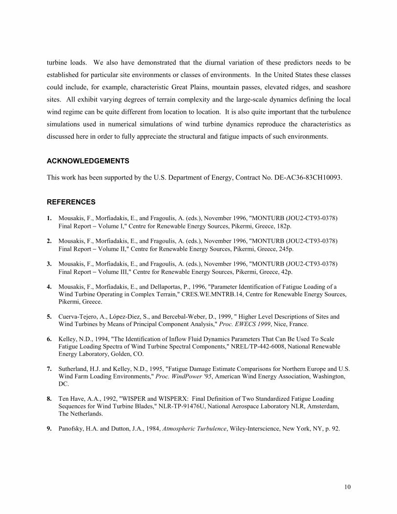
This increased damage can be further substantiated by noting that the cluster of peak Leq loads for m=10

and m=12 in Figure 1 occur at values exceeding 20 kNm. We determined that there are 16 10-minute

records contained within this cluster, whose associated mean wind speed ranged from 12.25 to 15.09 m/s.

Excluding the elements of this cluster, we searched the remaining database for records whose mean wind

speeds fell within this range. We found that there were 49 records of the remaining 381 available that met

this criteria. We then summarized the individual load spectra associated with the records of the peak

cluster and 49 other records from both turbine rotors into two composite spectra. Best-fit curves were

regressed through each of these spectra and the results plotted as a function of cycles per hour (see Figure

2). These curves indicate why the Leq peaks with high values of the S-N slope parameter occurred. The

inflow conditions associated with these 16 records contained elements that produced a greater number of

high-amplitude cycles than were characteristic of the other 49 records measured within the same wind

speed range. Because Figure 1 indicates a strong dependency on the Richardson number, we plotted the

distributions of this parameter for each of the above cases in Figure 3. This figure shows that the Leq

distribution associated with the high-damage cluster tends to be narrow and uni-modal. It is centered

between 21 and 22 h, with the bulk of the occurrences in the range of 20 to 22 h. The Leq distribution of

the 49 records with lower peaks is much broader and bi-modal and is centered between 22 and 23 h with

peaks at 21 and 01 h. Therefore, the higher fatigue damage for materials with high S-N slopes occurred

earlier in the transition from the daytime to the nocturnal boundary layer structure. Such damage is

therefore strongly diurnally related.

Sensitivity to Hub-Height Friction Velocity, u*

The other parameter that we identified in our earlier work [6] as an efficient predictor of low-cycle

turbine load behavior was the hub-height friction velocity, or u*. Figure 4 presents the variation of the

three-blade averaged Leq loads for m=12 for each rotor and the corresponding hub-height u* values as a

function of the turbine-layer Richardson number. Again, there is an abrupt change in both the Leq loads

7

on the rotors and u* as the stability transitions from unstable to stable. The high u* and Leq load regime

continues until an Ri value of approximately +0.10 is reached, whereas much lower values are evident in

the Ri down to −0.10. Thus, for the operating environment in this particular site, the number of operating

hours within a critical Ri range of 0 to +0.10 will see increased fatigue damage, particularly for blades

made of high S-N exponent material. This is consistent with the findings of a study by Sutherland and

Kelley [7], who compared the measured load spectrum from Rotor 1 with the WISPER spectrum [8].

They found that the San Gorgonio load spectrum contains many more cycles than the WISPER spectrum,

and that the increased number of cycles results in more damage. The higher loads and damage at San

Gorgonio are attributed to a combination of boundary-layer flows interacting with the complex terrain and

upstream turbine wakes.

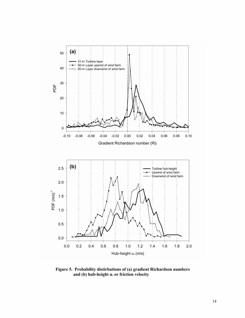
Distributions of Richardson number and u* at Other Locations at this Site

In 1989 we made extensive turbulence measurements from two 50-meter towers located upwind of Row 1

and downwind of the last turbines of Row 41 using similar but more sensitive instrumentation. The total

records from each location are much more extensive than those that were available from Row 37 in 1990.

The majority of the measurements were made earlier in the wind season, covering a six-week period

approximately from early June to mid July that was characterized by periods of strong winds. There were

no turbines upwind of Row 1 and the closest operating row to Row 41 was approximately 14 rotor

diameters (D) upstream. In Figures 5a and 5b we compared the distributions of the gradient Richardson

number and the hub-height u* for the upstream, downstream, and Row 37 locations. respectively in

Figures 5a and 5b. Figure 5a shows the predominance of operation in the weakly stable region for both

the upwind (Row 1) and downwind locations. There is a small, secondary peak at the downwind station

and 14-D spacing that coincides with the primary peak at Row 37. In general, the Ri distribution at Row

37 peaks at a slightly more stable value and is much broader than the distributions at the other two

locations in the stable region. In comparison with the other two layers, the shallower depth of the Ri

measurement layer at Row 37 may have more influence than the other two. The impact of the presence of

upstream turbine wakes is clearly visible in the u* distributions. The median value for the upwind

location is 0.771 m/s, 1.106 m/s downwind of Row 41, and 1.161 m/s for Row 37, with the tail reaching

values in excess of 1.800 m/s. Thus, from the Ri and u* distributions shown in Figures 5a and 5b, one

would expect the highest fatigue damage at Row 37 and the least from the turbines installed in Row 1.

This scenario is essentially what the wind farm operator has observed.

8

DIURNAL VARIATION AS AN IMPORTANT PARAMETER

One of most sensitive factors affecting thermodynamic-related turbulence descriptors is the time-of-day

(or diurnal) variation (see Figure 3). The daily heating and cooling cycle of the earth's boundary layer is a

major source of variation. This is true in most locations except, of course, in arctic regions during periods

with little or no sunlight reaching the usually snow covered surface. Even here thermodynamics may still

be important, because very strong inversions often exist with much warmer air aloft that is occasionally

brought to the surface through some form of intrusion process. The diurnal heating and cooling of

complex terrain features is known to alter the flow characteristics around such obstacles.

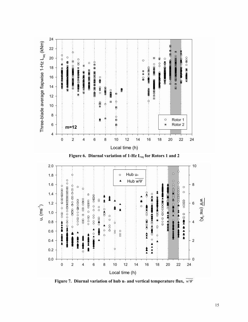
In Figure 6 we plotted the diurnal variation of the three-blade average 1-Hz Leq loads using m=12 for each

of the two rotors in the San Gorgonio wind farm. The shaded region between 20 and 22 h corresponds to

the period where the majority of the peak loads were observed, as discussed earlier. The distribution of

Leq loads is strongly diurnal and follows the hourly variation in mean wind speed. This profile is largely

controlled by the large-scale dynamics of the region, which are modulated by the complex terrain features

(i.e., the mountains and the pass). The strongest winds tend to occur two or three hours after local sunset

when the boundary layer is in the process of transitioning from the day to night boundary layer structure.

Between 10 and 15 h the wind generally drops below power generation levels as (see Figure 6).

The diurnal relationship between the thermal field and the hub-height mean shearing stress or u* is shown

in Figure 7. We plotted the variation of u* (dotted circles) and the covariance of the fluctuating vertical

velocity component and potential temperature, which is the vertical temperature flux (filled triangles). A

positive temperature flux indicates that heat is being transported away from the surface. The period of

sunrise is clearly visible between 06 and 08 h with a strong, positive temperature flux readily evident.

Local sunset is between about 19 and 20 h on this diagram. At approximately 19 h the vertical

temperature flux reaches a maximum for the day, at the same time the sun is setting. This indicates the

presence of a strong, positive, vertical velocity field transporting a net heat flow into the boundary layer.

Immediately after this peak, the u* increases rapidly as the temperature flux falls at more or less the same

rate. It is during this approximately one-hour period that turbulence production changes from one

dominated by buoyant plumes to shear production. Very intense, transient coherent turbulent structures

exist in regions of strong vertical velocity fields and rapidly changing shears.

The processes described here are further documented by the diurnal variation of the Richardson number

and u* plotted in Figure 8. Again, the transitions at sunrise and sunset are well characterized by the Ri

9

and u* variations. The strong vertical temperature (heat) flux after sunrise quickly destabilizes the

boundary layer through positive buoyancy while the shear (u*) contribution falls, resulting in large

negative Ri values. At sunset the inverse occurs with an increasingly stabilizing boundary layer and an

increase in the shear which causes the value of Ri to become slightly positive. After about 21 h, the shear

becomes the dominant turbulence source damped by a small amount of negative buoyancy, as indicated

by the small positive values of Ri. Early in the morning after about 02 h, the Ri begins to rise and the

turbulence becomes further damped as the wind speed and shearing stress decrease before reaching a

minimum just before sunrise. The diurnal variation of the 1-Hz Leq loads shown in Figure 6 closely

mirrors the variation of Ri and u* of Figure 8; i.e., a combination of negative Ri and low u* values leads to

low Leq. Conversely, during the day-night transition when u* is high and the Ri weakly positive, the Leq

are high and damaging. The variations in the velocity and thermodynamic fields of Figure 7 show why it

is necessary to consider both when assessing the efficiency of turbulent load predictor variables.

The processes discussed above are quantified by the turbulent kinetic-energy budget equation given by

Panofsky and Dutton [9]:

( ) ( ) ( ) ( ) ( ) εθθ

εθθ

−∂∂−+

∂∂=−

∂∂−+

∂∂−=

∂∂= Ew'

z'w'

g

z

uuEw'

z'w'

g

z

u'w'u

E

Dt

ED 2*t

In this equation, the pressure correction term and the effects of moisture were ignored. E is the total

kinetic energy given by E = (1/2) (u'2 + v'2 + w'2) and ε is the dissipation rate of turbulent kinetic energy.

The first term (I) of the terms on the right is the shear production term and is always positive. The second

term (II) is the buoyancy production term and may be positive or negative depending on the sign of the

vertical temperature flux 'w'θ . The values of 'w'θ shown in Figure 7 never go negative because of the

high surface temperatures in July and August. The third term (III) defines the rate at which turbulence is

transported into or out of the local volume by velocity fluctuations. This equation couples the importance

of the velocity and thermodynamic fields and the related scaling quantities. In a wind farm environment,

the third term on the right may be very important due to the transport of upwind turbine wakes.

CONCLUSIONS

In this paper we have underscored the need to include atmospheric thermodynamic variables, such as a

measure of vertical stability, when identifying efficient predictors for evaluating turbulence-induced wind

I II III I II III

10

turbine loads. We also have demonstrated that the diurnal variation of these predictors needs to be

established for particular site environments or classes of environments. In the United States these classes

could include, for example, characteristic Great Plains, mountain passes, elevated ridges, and seashore

sites. All exhibit varying degrees of terrain complexity and the large-scale dynamics defining the local

wind regime can be quite different from location to location. It is also quite important that the turbulence

simulations used in numerical simulations of wind turbine dynamics reproduce the characteristics as

discussed here in order to fully appreciate the structural and fatigue impacts of such environments.

ACKNOWLEDGEMENTS

This work has been supported by the U.S. Department of Energy, Contract No. DE-AC36-83CH10093.

REFERENCES

1. Mousakis, F., Morfiadakis, E., and Fragoulis, A. (eds.), November 1996, "MONTURB (JOU2-CT93-0378)Final Report − Volume I," Centre for Renewable Energy Sources, Pikermi, Greece, 182p.

2. Mousakis, F., Morfiadakis, E., and Fragoulis, A. (eds.), November 1996, "MONTURB (JOU2-CT93-0378)Final Report − Volume II," Centre for Renewable Energy Sources, Pikermi, Greece, 245p.

3. Mousakis, F., Morfiadakis, E., and Fragoulis, A. (eds.), November 1996, "MONTURB (JOU2-CT93-0378)Final Report − Volume III," Centre for Renewable Energy Sources, Pikermi, Greece, 42p.

4. Mousakis, F., Morfiadakis, E., and Dellaportas, P., 1996, "Parameter Identification of Fatigue Loading of aWind Turbine Operating in Complex Terrain," CRES.WE.MNTRB.14, Centre for Renewable Energy Sources,Pikermi, Greece.

5. Cuerva-Tejero, A., López-Diez, S., and Bercebal-Weber, D., 1999, " Higher Level Descriptions of Sites andWind Turbines by Means of Principal Component Analysis," Proc. EWECS 1999, Nice, France.

6. Kelley, N.D., 1994, "The Identification of Inflow Fluid Dynamics Parameters That Can Be Used To ScaleFatigue Loading Spectra of Wind Turbine Spectral Components," NREL/TP-442-6008, National RenewableEnergy Laboratory, Golden, CO.

7. Sutherland, H.J. and Kelley, N.D., 1995, "Fatigue Damage Estimate Comparisons for Northern Europe and U.S.Wind Farm Loading Environments," Proc. WindPower '95, American Wind Energy Association, Washington,DC.

8. Ten Have, A.A., 1992, "WISPER and WISPERX: Final Definition of Two Standardized Fatigue LoadingSequences for Wind Turbine Blades," NLR-TP-91476U, National Aerospace Laboratory NLR, Amsterdam,The Netherlands.

9. Panofsky, H.A. and Dutton, J.A., 1984, Atmospheric Turbulence, Wiley-Interscience, New York, NY, p. 92.

11

m=4

Fla

pw

ise

1-H

z L

eq (

kNm

)

2

4

6

8

10

12

14

16

18

20

22

24

m=4

Fla

pw

ise

1-H

z L

eq (

kNm

)

2

4

6

8

10

12

14

16

18

20

22

24

Rotor 1Rotor 2

m=6

Pea

k fl

apw

ise

1-H

z L

eq (

kNm

)

2

4

6

8

10

12

14

16

18

20

22

24

m=8

Fla

pw

ise

1-H

z L

eq (

kNm

)

2

4

6

8

10

12

14

16

18

20

22

24

m=10

Fla

pw

ise

1-H

z L

eq (

kNm

)

2

4

6

8

10

12

14

16

18

20

22

24

m=12

Turbine-layer gradient Richardson number (Ri)

-0.4 -0.3 -0.2 -0.1 0.0 0.1 0.2

Fla

pw

ise

1-H

z L

eq (

kNm

)

2

4

6

8

10

12

14

16

18

20

22

24

m=6

Fla

pw

ise

1-H

z L

eq (

kNm

)

2

4

6

8

10

12

14

16

18

20

22

24

m=8F

lap

wis

e 1-

Hz

Leq

(kN

m)

2

4

6

8

10

12

14

16

18

20

22

24

m=10

Fla

pw

ise

1-H

z L

eq (

kNm

)

2

4

6

8

10

12

14

16

18

20

22

24

m=12

Turbine-layer gradient Richardson number (Ri)

-0.4 -0.3 -0.2 -0.1 0.0 0.1 0.2

Fla

pw

ise

1-H

z L

eq (

kNm

)

2

4

6

8

10

12

14

16

18

20

22

24

Three-Blade Peak 1-Hz Leq Three-Blade Average 1-Hz Leq

Figure 1. Variation of three-blade peak and average 1-Hz Leq loads with the Richardsonnumber stability parameter

12

.Cycles/h

1 10 100 1000 10000

Alte

rnatin

g a

mplit

ude (

kNm

)

0

5

10

15

20

25

30

35

40

Peak 1Hz Leq > 20 kNm

Peak 1Hz Leq ≤ 20 kNm

Figure 2. Comparison of peak load cases

1 2 3 4 5 6 7

Local time (h)

15 16 17 18 19 20 21 22 23 24

Pe

rce

nta

ge

of

reco

rds

in lo

adin

g g

rou

p

0

5

10

15

20

25

30

35

Peak Leq ≤ 20 kNm

Peak Leq > 20 kNm

Figure 3. Time distributions of peak loading groups

13

Turbine-layer gradient Richardson number (Ri)

-0.4 -0.3 -0.2 -0.1 0.0 0.1 0.2

Hub u

* (m

/s)

0.2

0.4

0.6

0.8

1.0

1.2

1.4

1.6

1.8

2.0

2.2 Thre

e-b

lade a

vera

ge fla

pw

ise 1

-Hz L

eq (kNm

)

4

6

8

10

12

14

16

18

20

22

24

Hub u*

Leq Rotor 1

Leq Rotor 2

m=12

Figure 4. Variation of hub u* and average 1-Hz Leq with stability

14

Hub-height u* (m/s)

0.0 0.2 0.4 0.6 0.8 1.0 1.2 1.4 1.6 1.8 2.0

PD

F (

m/s

)-1

0.0

0.5

1.0

1.5

2.0

2.5

Gradient Richardson number (Ri)

-0.10 -0.08 -0.06 -0.04 -0.02 0.00 0.02 0.04 0.06 0.08 0.10

PD

F

0

10

20

30

40

50

Turbine hub-heightUpwind of wind farmDownwind of wind farm

(a)

(b)

31-m Turbine layer50-m Layer upwind of wind farm50-m Layer downwind of wind farm

Figure 5. Probability distirbutions of (a) gradient Richardson numbers and (b) hub-height u* or friction velocity

15

Local time (h)

0 2 4 6 8 10 12 14 16 18 20 22 24

Th

ree

-bla

de

ave

rage

fla

pw

ise

1-H

z L

eq (

kNm

)

4

6

8

10

12

14

16

18

20

22

24

Rotor 1Rotor 2

m=12

Figure 6. Diurnal variation of 1-Hz Leq for Rotors 1 and 2

Local time (h)

0 2 4 6 8 10 12 14 16 18 20 22 24

u* (

ms-1

)

0.0

0.2

0.4

0.6

0.8

1.0

1.2

1.4

1.6

1.8

2.0

w'θ ' (m

s-1K

)

0

2

4

6

8

10

Hub w'θ'

Hub u*

Figure 7. Diurnal variation of hub u* and vertical temperature flux, 'w'θ

16

Local time (h)

0 2 4 6 8 10 12 14 16 18 20 22 24

u* (

ms-1

)

0.0

0.2

0.4

0.6

0.8

1.0

1.2

1.4

1.6

1.8

2.0 Tu

rbin

e-la

yer g

rad

ien

t Rich

ard

son

nu

mb

er (R

i)

-0.4

-0.3

-0.2

-0.1

0.0

0.1

0.2

0.3

Hub u*

Ri

Ri = 0, neutral

Figure 8. Diurnal variation of Richardson number and hub-height u*