A CALIBRATED, HIGH-RESOLUTION GOES SATELLITE SOLAR INSOLATION

A CALIBRATED, HIGH-RESOLUTION GOES SATELLITE SOLAR INSOLATIONPRODUCT FOR A CLIMATOLOGY OF FLORIDA EVAPOTRANSPIRATION1

Simon J. Paech, John R. Mecikalski, David M. Sumner, Chandra S. Pathak,

Quinlong Wu, Shafiqul Islam, and Taiye Sangoyomi2

ABSTRACT: Estimates of incoming solar radiation (insolation) from Geostationary Operational EnvironmentalSatellite observations have been produced for the state of Florida over a 10-year period (1995-2004). These insola-tion estimates were developed into well-calibrated half-hourly and daily integrated solar insolation fields over thestate at 2 km resolution, in addition to a 2-week running minimum surface albedo product. Model results of thedaily integrated insolation were compared with ground-based pyranometers, and as a result, the entire datasetwas calibrated. This calibration was accomplished through a three-step process: (1) comparison with ground-basedpyranometer measurements on clear (noncloudy) reference days, (2) correcting for a bias related to cloudiness, and(3) deriving a monthly bias correction factor. Precalibration results indicated good model performance, with astation-averaged model error of 2.2 MJ m)2 ⁄ day (13%). Calibration reduced errors to 1.7 MJ m)2 ⁄ day (10%), andalso removed temporal-related, seasonal-related, and satellite sensor-related biases. The calibrated insolation data-set will subsequently be used by state of Florida Water Management Districts to produce statewide, 2-km resolu-tion maps of estimated daily reference and potential evapotranspiration for water management-related activities.

(KEY TERMS: solar insolation; evapotranspiration; remote sensing; water resources management; referenceevapotranspiration; Penman-Monteith.)

Paech, Simon J., John R. Mecikalski, David M. Sumner, Chandra S. Pathak, Quinlong Wu, Shafiqul Islam, andTaiye Sangoyomi, 2009. A Calibrated, High-Resolution GOES Satellite Solar Insolation Product for a Climatol-ogy of Florida Evapotranspiration. Journal of the American Water Resources Association (JAWRA) 45(6):1328-1342. DOI: 10.1111/j.1752-1688.2009.00366.x

INTRODUCTION

Estimates of incoming solar radiation (insolation)from satellite data for the state of Florida over a 10-year period (June 1, 1995 to December 31, 2004) havebeen produced for use by state of Florida Water Man-agement Districts (WMD) for evapotranspiration (ET)

estimation using a Penman-Monteith technique (Pen-man, 1948; Monteith, 1965). For producing referenceET, the Penman-Monteith relationship is usedtogether with ‘‘crop coefficient’’ values. Solar insola-tion is the largest determinant for temporal variationin ET, which is a critical variable for water manage-ment, both in hydrologic flow simulations (involvingpotential ET) and water allocation and agricultural

1Paper No. JAWRA-08-0132-P of the Journal of the American Water Resources Association (JAWRA). Received July 7, 2008; accepted July7, 2009. ª 2009 American Water Resources Association. No claim to original U.S. government works. Discussions are open until sixmonths from print publication.

2Respectively, Research Associate and Assistant Professor (Paech and Mecikalski), Department of Atmospheric Sciences, University ofAlabama in Huntsville, Huntsville, Alabama; Hydrologist (Sumner), U.S. Geological Survey, Florida Integrated Science Center, Orlando,Florida; Principal Engineer, Senior Engineer, and Lead Engineer (Pathak, Wu, and Sangoyomi), Operations and Hydro Data ManagementDivision, South Florida Water Management District, West Palm Beach, Florida; and Professor (Islam), Department of Civil and Environmen-tal Engineering, Tufts University, Medford, Massachusetts (E-Mail ⁄ Paech: [email protected]).

JAWRA 1328 JOURNAL OF THE AMERICAN WATER RESOURCES ASSOCIATION

JOURNAL OF THE AMERICAN WATER RESOURCES ASSOCIATION

Vol. 45, No. 6 AMERICAN WATER RESOURCES ASSOCIATION December 2009

water use (involving reference ET). The most desir-able ET datasets for these purposes are spatially con-tinuous, rather than point values derived fromtraditional field station networks, thus statewidemapping of ET is greatly facilitated by satellite-derived estimates of the spatial distribution of solarinsolation. To date, the five Florida WMD have nothad access to a common source of solar insolationdata or methodologies for calculating the two mostwidely used indicators of ET (potential and referenceET). The motivation of this work is to develop arobust insolation calibration framework coupled to asatellite-based insolation model, so to provide for keyradiative datasets for the formulation of a 10-yearlong, ET climatology (which will extend indefinitelyinto the future). These insolation datasets are used inconjunction with other information, such as net radi-ation, soil heat flux, and temporally varying cropcoefficients, in the formulation of ET. This paperfocuses only on the development of the insolationdata, and subsequent calibration activities, demon-strating the powerful utility of satellite-derived fieldsfor water resource applications.

Applications of a high-resolution (£5 km) solarinsolation dataset include its use in the developmentof reference ET and potential ET. Reference ET isvaluable for irrigation scheduling and water manage-ment, while potential ET can be used as input intosurface and groundwater hydrological models,whereas the solar insolation data themselves may beused as boundary conditions in certain ecosystemmodels. Clearly, geostationary satellites provide spa-tially and temporally continuous data across allregions in their view (between approximately ±55�latitude), a huge advantage over ground-based instru-mentation. Use of a satellite-based insolation algo-rithm also ensures that a consistent algorithm isapplied across an entire region.

Satellite visible data have been used for estimatingsolar insolation for a number of years, with methodsranging from statistical-empirical relationships suchas Tarpley (1979), to physical models of varying com-plexity (see Gautier et al., 1980, 1984; Diak and Gau-tier, 1983; Moser and Raschke, 1984; Pinker andEwing, 1985; Dedieu et al., 1987; Darnell et al., 1988;Frouin and Chertock, 1992; Pinker and Laszlo, 1992;Weymouth and LeMarshall, 1999). Studies such asSchmetz (1989) and Pinker et al. (1995) have proventhe utility of satellite-estimated solar insolationmethods, showing that such models produce fairlyaccurate results – with hourly insolation estimateswithin 5-10% of pyranometer data during clear-skyconditions (15-30% for all sky conditions) and dailyestimates within 10-15%. Additional works such asthose of Stewart et al. (1999) and Otkin et al. (2005)have further bolstered the utility of this technique.

Advantages of using satellite-estimated insolationdata over those collected by pyranometer networksinclude large spatial coverage; high spatial resolu-tion; the availability of data in remote, inaccessible,or potentially hazardous regions, over oceans andlarge water bodies (e.g., Frouin et al., 1988); and incountries that may not have the means to install aground-based pyranometer network.

A similar effort to that developed here for estimat-ing solar insolation from satellite is described by Cos-grove et al. (2003a,b). In these studies, use of theGlobal Energy and Water Cycle Experiment (GEW-EX) Surface Radiation Budget (SRB) downward solarflux algorithm (Pinker and Laszlo, 1992) has beendemonstrated within the North American Land DataAssimilation project. The error statistics for the SRBproduct are comparable to those shown via this study(see Model Calibration), while the resolution of theSRB solar flux data are 0.5� resolution (see Menget al., 2003). The main reason for not using SRB hereis that the needed resolution deemed important forestimating ET over Florida was on or near the cumu-lus cloud scale, namely 1-3 km, far above that of SRBdata. SRB data are developed from a combination ofpolar orbiting and geostationary satellite data, whilethe solar insolation fields described here are devel-oped only from Geostationary Operational Environ-mental Satellite (GOES) data. A more thoroughdescription of the GEWEX SRB data is available athttp://www.gewex-srb.larc.nasa.gov.

Other limitations for much of this previous workhave been centered around the need for informationon atmospheric parameters that limit the effective-ness of these models, such as aerosols and precipita-ble water (PW) information. Problems associated withassessing the performance of these models are oftenfraught with issues related to scale differencesbetween point observations and satellite pixel resolu-tion (from �1 to 4 km). Satellite sensor degradation,especially prevalent on the National Oceanic andAtmospheric Administration (NOAA) GOES satelliteseries, are often difficult to quantify, albeit it is oneaspect this study attempts to address.

In this study, data from the NOAA GOES ‘‘East’’series of satellites are used. GOES data wereobtained from the GOES data archive at the SpaceScience and Engineering Center at the University ofWisconsin-Madison. Approximately 102,000 individ-ual GOES images were processed for this effort.These data were processed using the model of Gau-tier et al. (1980) to produce half-hourly and dailyintegrated solar insolation and 2-week running mini-mum surface albedo data throughout the state ofFlorida at 2-km horizontal spatial resolution. Asnoted above, this high-resolution was chosen to pro-vide solar insolation observations between cumulus

A CALIBRATED, HIGH-RESOLUTION GOES SATELLITE SOLAR INSOLATION PRODUCT FOR A CLIMATOLOGY OF FLORIDA EVAPOTRANSPIRATION

JOURNAL OF THE AMERICAN WATER RESOURCES ASSOCIATION 1329 JAWRA

clouds, which comprise a significant component ofFlorida’s cloud climatology.

The other unique aspect of this work involved anextensive model calibration activity for the insolationproduct, undertaken by comparing satellite-derivedinsolation estimates to that of ground-based pyra-nometers and clear-sky radiation models. This com-parison provided information to tune or adjust biasesin the daily integrated insolation dataset for localenvironmental conditions. This was achieved via athree-step process: (1) comparison with ground-basedpyranometer measurements on clear (noncloudy) ref-erence days, (2) correcting for a bias related to cloudi-ness, and (3) deriving a monthly bias correctionfactor. This resulted in a significant reduction in biaserrors and henceforth the formation of a very robustET product.

The goal of this paper is to describe the productionand calibration of a 2 km GOES-based insolationproduct, for eventual applications related to watermanagement and ET. The approach is deemed sim-ple, and once bias corrections are determined, insola-tion data with good error statistics without need forancillary datasets are the result. The paper proceedsas follows: The Solar Insolation Model section of thispaper provides an overview of the insolation model;Data Acquisition, Processing, and Quality Controlsection discusses data acquisition, processing, andquality control; Model Calibration details themodel calibration efforts; followed by Discussion ofCalibration Issues; and Summary and Conclusion,respectively.

THE SOLAR INSOLATION MODEL

The model developed by Gautier et al. (1980) [withmodifications by Diak and Gautier (1983) andupdated application methods by Diak et al. (1996),from this point onwards referred to as the ‘‘GDM’’]employs a fairly simple physical representation ofcloud and atmosphere radiative processes, yet hasbeen shown to perform as well as, or even betterthan, more complex methods over a variety of land-surface and climatic conditions (Gautier et al., 1984;Raphael and Hay, 1984; Frouin et al., 1988; Diaket al., 1996; Jacobs et al., 2002, 2004; Otkin et al.,2005). When comparing with pyranometer data, thesestudies reported root mean square errors (RMSEs) inhourly and daily insolation estimates (as a percent-age of the mean pyranometer observed value) from17 to 28 and 9 to 10%, respectively. The high ends ofthese errors (�28 and �10%, respectively) werereported in the study of Jacobs et al. (2002), which

took place over northern-central Florida and wascharacterized by significant convective-cloud activity.The GDM has also been proven in operational use,producing near-real-time insolation estimates forregional-scale and continental-scale land-surface car-bon and water flux assessments (Mecikalski et al.,1999; Anderson et al., 2003, 2004), subsurface hydro-logic modeling, and the generation of agriculturalforecasting products (Diak et al., 1998; Andersonet al., 2001). A full description of the GDM is givenby Gautier et al. (1980), Diak and Gautier (1983),and Diak et al. (1996) – a basic overview is givenhere.

The model is based on conservation of radiantenergy in the Earth-atmosphere column. The GDMhas two modes for determining solar insolationreceived at the Earth’s surface: one for clear and onefor cloudy conditions, based on satellite-inferred sur-face albedo data. A running 2-week minimum of thisalbedo data, reassessed at solar noon daily, is storedfor each GOES visible data pixel, yielding a referencealbedo grid representative of clear-sky conditions andcapturing temporal changes in land-surface charac-teristics. This approach represents the true land-sur-face albedo more accurately than using the dailyestimated value because the latter can be corruptedby high albedo values when clouds are present duringthe course of a day. [It should be noted that this min-imum albedo product is wavelength-specific, uniqueto the GOES visible sensor (which does in factinclude contributions from the near infrared), andtherefore does not represent a true surface albedo.]

Within the GDM, for a given GOES image, the dig-ital brightness at each image pixel is compared tothat of the stored clear-sky reference albedo data forthat pixel. If the brightness exceeds a given threshold[a function of the 2-week running minimum noontimealbedo; Diak and Gautier (1983)], the pixel is deemedcloudy, and vice versa. Based on this determination,either a clear or cloudy model of atmospheric radia-tion processes is used to calculate solar insolationreceived at the surface, for each pixel. Both the clearand cloudy models incorporate parameterizations forozone absorption, Raleigh scattering, and water vaporabsorption within the atmospheric column using sim-ple bulk relationships – the use of fixed ozone andaerosol contents being sufficient given that these pro-duce secondary, smaller sources of error. The cloudyGDM component estimates a cloud-top albedo, andaccounts for atmospheric effects above and below thecloud separately.

For the water vapor absorption parameterization,a fixed, approximate annual median value of 3.0 cmwas used to estimate atmospheric column-integratedPW during the initial processing. [PW is defined asthe amount of water that would precipitate out of a

PAECH, MECIKALSKI, SUMNER, PATHAK, WU, ISLAM, AND SANGOYOMI


vertical column of the atmosphere if all the watervapor were condensed into liquid.] PW data areneeded to calculate the slantwise path, and subse-quently the absorption coefficients in the Gautieret al. (1980) method. Postprocessing adjustmentswere then made to account for diurnal variations ofPW (i.e., PW values greater or less than the 3.0 cmmedian value), given the logistical difficulty of includ-ing these data within the modeling stage. Theseadjustments were made by deriving diurnal adjust-ment factors based on daily representative PW valuesover Florida from numerical weather prediction(NWP) model data [National Centers for Environmen-tal Prediction reanalysis dataset (NOAA ⁄ OAR ⁄ ESRLPSD, Boulder, Colorado; http://www.cdc.noaa.gov)]. Inmany instances, daily PW values over Florida werewell above 3.0 cm, certainly during summer, whilewintertime values were often much lower. Noaccounting was made for daily variations in PW con-sidering the relatively small amount of inter-day var-iability that typically occurs over Florida, especiallyduring summer, and because this would haverequired a reliance on forecasts from these models,which are often incorrect. We also do not account formeso-c scale (2-25 km) scale variations in PW giventhis would require substantially larger amounts ofmodel-derived data. Data from NWP models wouldneed to be incorporated if constructing similar insola-tion climatologies for regions outside Florida withvery high daily variations in PW.

DATA ACQUISITION, PROCESSING,AND QUALITY CONTROL

GOES Satellite Data

The GOES East series of satellites (the most recentadditions being GOES-8 and GOES-12) have beenplaced in geostationary orbit above the Earth’s equatorat longitude 75�W, providing continuous observationsin several visible and nonvisible radiation bands ofmuch of the western hemisphere at high spatial(‡1 km) and temporal (‡15 min) resolution, makingdata collected by them ideal for high-resolution esti-mates of solar insolation. During the time periodspanned by this study, the GOES-8 satellite (launchedin April 1994) was decommissioned and the GOES-12satellite took its place on April 1, 2003. Data from bothof these satellites were acquired and utilized.

Although the GOES visible sensors have a nadir(the point directly below the satellite) spatial resolu-tion of 1 km, this resolution decreases the furtherfrom nadir the instrument scans: for the state of

Florida region, the highest resolution attainable isabout 1.5-2.0 km. This was the input and output res-olution of the GDM in this work. Half-hourly solarinsolation values were calculated using GOES datafrom 15 and 45 min past the hour, and daily valueswere calculated by integrating the half-hourly valuesover the period of daylight (using the trapezoidalintegration method). A simple method for computingsunrise and sunset times per pixel across the domainwas used. The running 2-week minimum albedo prod-uct discussed in the section The Solar InsolationModel was calculated using data at solar noon. Theseproducts were generated both in the original satelliteprojection, and translated to a grid identical to thatused for the Statewide NEXRAD radar-derived rain-fall estimation product (Hoblit et al., 2003). In thelatter dataset, the data were interpolated in time to00 and 30 min past the hour.

Potential GOES data issues include sensor degra-dation with time and sun glint effects (i.e., the reflec-tion of the Sun’s disk from land and sea surfaces).The effects of the latter are small, and not addressedin this study due to the complexity of the phenomena.Sensor degradation is addressed and corrected forthrough the calibration of the product, detailed in fol-lowing sections. This issue is also discussed furtherin the section titled Discussion of Calibration Issues.

In general, GOES satellite data are available on acontinual basis with high reliability. Under specificconditions though, the instruments are shut down(for example when sunlight shines directly into thesensors), and other issues such as receiving-stationglitches can result in the occasional loss or corruptionof an image or series of images. For this reason, ifmore than five half-hourly satellite images were miss-ing on a given day, the daily insolation value for thatday (being derived from the half-hourly data) wasflagged as unusable. Days with three to five missingimages were designated usable, and those with zeroto two missing images were designated as good qual-ity data. Where there were gaps in the usable data,linear interpolation was used to fill them. (The finalinsolation product includes flags for data loss.)

Pyranometer Data

Pyranometer data used to calibrate the satelliteisolation product, and subsequently assess calibrationperformance, were obtained from a number ofweather stations networks across Florida, each main-tained by a different agency. The state of Florida isdivided into five regional WMDs: Northwest Florida(NWF), South Florida (SF), St. Johns River (SJR),Suwannee River (SR), and Southwest Florida (SWF)as shown in Figure 1. Historical pyranometer data



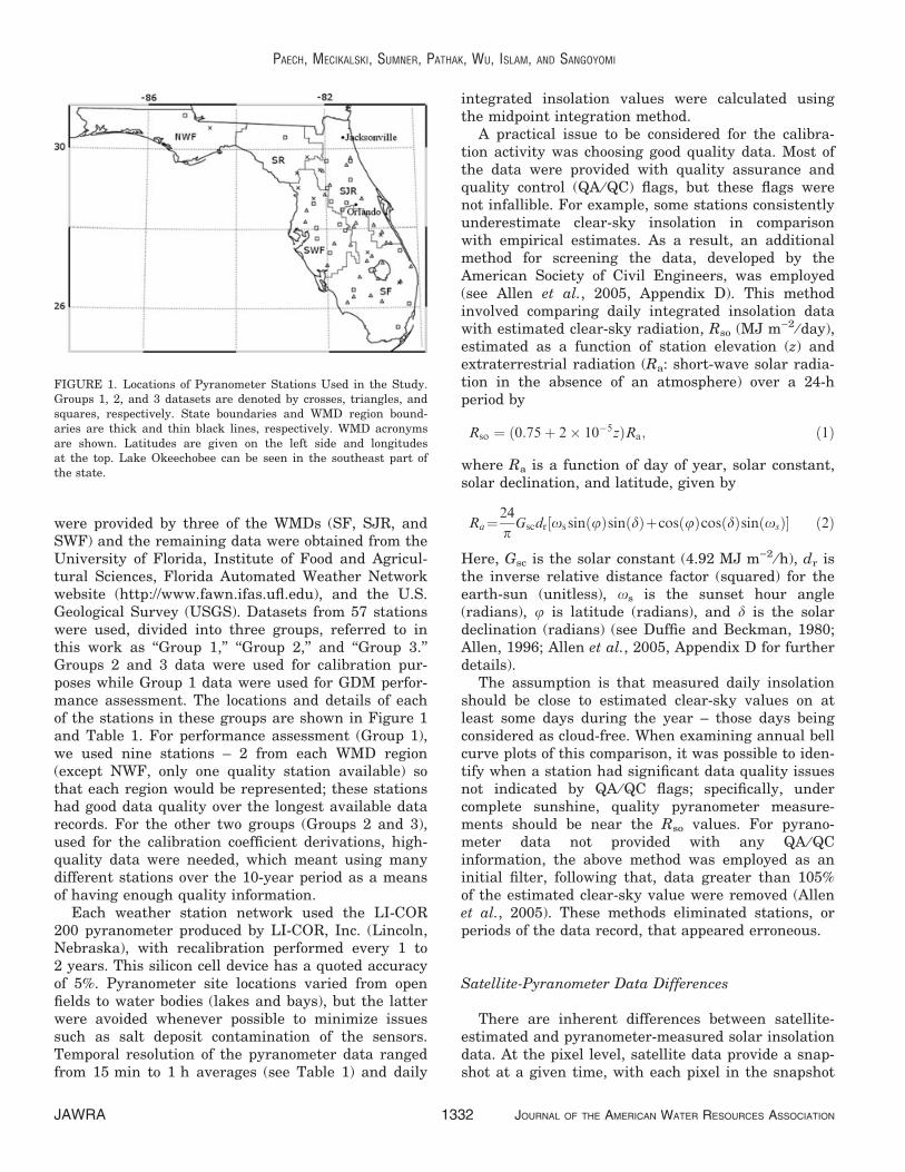
were provided by three of the WMDs (SF, SJR, andSWF) and the remaining data were obtained from theUniversity of Florida, Institute of Food and Agricul-tural Sciences, Florida Automated Weather Networkwebsite (http://www.fawn.ifas.ufl.edu), and the U.S.Geological Survey (USGS). Datasets from 57 stationswere used, divided into three groups, referred to inthis work as ‘‘Group 1,’’ ‘‘Group 2,’’ and ‘‘Group 3.’’Groups 2 and 3 data were used for calibration pur-poses while Group 1 data were used for GDM perfor-mance assessment. The locations and details of eachof the stations in these groups are shown in Figure 1and Table 1. For performance assessment (Group 1),we used nine stations – 2 from each WMD region(except NWF, only one quality station available) sothat each region would be represented; these stationshad good data quality over the longest available datarecords. For the other two groups (Groups 2 and 3),used for the calibration coefficient derivations, high-quality data were needed, which meant using manydifferent stations over the 10-year period as a meansof having enough quality information.

Each weather station network used the LI-COR200 pyranometer produced by LI-COR, Inc. (Lincoln,Nebraska), with recalibration performed every 1 to2 years. This silicon cell device has a quoted accuracyof 5%. Pyranometer site locations varied from openfields to water bodies (lakes and bays), but the latterwere avoided whenever possible to minimize issuessuch as salt deposit contamination of the sensors.Temporal resolution of the pyranometer data rangedfrom 15 min to 1 h averages (see Table 1) and daily

integrated insolation values were calculated usingthe midpoint integration method.

A practical issue to be considered for the calibra-tion activity was choosing good quality data. Most ofthe data were provided with quality assurance andquality control (QA ⁄ QC) flags, but these flags werenot infallible. For example, some stations consistentlyunderestimate clear-sky insolation in comparisonwith empirical estimates. As a result, an additionalmethod for screening the data, developed by theAmerican Society of Civil Engineers, was employed(see Allen et al., 2005, Appendix D). This methodinvolved comparing daily integrated insolation datawith estimated clear-sky radiation, Rso (MJ m)2 ⁄ day),estimated as a function of station elevation (z) andextraterrestrial radiation (Ra: short-wave solar radia-tion in the absence of an atmosphere) over a 24-hperiod by

Rso ¼ ð0:75þ 2� 10�5zÞRa; ð1Þ

where Ra is a function of day of year, solar constant,solar declination, and latitude, given by

Ra¼24

pGscdr½xs sin uð ÞsinðdÞþcosðuÞcosðdÞsinðxsÞ� ð2Þ

Here, Gsc is the solar constant (4.92 MJ m)2 ⁄ h), dr isthe inverse relative distance factor (squared) for theearth-sun (unitless), xs is the sunset hour angle(radians), u is latitude (radians), and d is the solardeclination (radians) (see Duffie and Beckman, 1980;Allen, 1996; Allen et al., 2005, Appendix D for furtherdetails).

The assumption is that measured daily insolationshould be close to estimated clear-sky values on atleast some days during the year – those days beingconsidered as cloud-free. When examining annual bellcurve plots of this comparison, it was possible to iden-tify when a station had significant data quality issuesnot indicated by QA ⁄ QC flags; specifically, undercomplete sunshine, quality pyranometer measure-ments should be near the Rso values. For pyrano-meter data not provided with any QA ⁄ QCinformation, the above method was employed as aninitial filter, following that, data greater than 105%of the estimated clear-sky value were removed (Allenet al., 2005). These methods eliminated stations, orperiods of the data record, that appeared erroneous.

Satellite-Pyranometer Data Differences

There are inherent differences between satellite-estimated and pyranometer-measured solar insolationdata. At the pixel level, satellite data provide a snap-shot at a given time, with each pixel in the snapshot

FIGURE 1. Locations of Pyranometer Stations Used in the Study.Groups 1, 2, and 3 datasets are denoted by crosses, triangles, andsquares, respectively. State boundaries and WMD region bound-aries are thick and thin black lines, respectively. WMD acronymsare shown. Latitudes are given on the left side and longitudesat the top. Lake Okeechobee can be seen in the southeast part ofthe state.



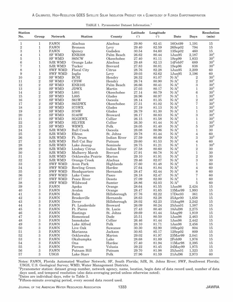
TABLE 1. Pyranometer Dataset Information.1

StationNo. Group Network Station County

Latitude(�)

Longitude(�) Date Days

Resolution(min)

1 1 FAWN Alachua Alachua 29.80 82.41 16Oct99 1,191 152 1 FAWN Bronson Levy 29.40 82.59 26Sep02 794 153 1 FAWN Quincy Gadsden 30.54 84.60 13Sep02 460 154 1 SF WMD ENR308 Palm Beach 26.62 80.44 1Jun95 2,187 303

5 1 SF WMD S65CW Okeechobee 27.40 81.11 1Sep99 1,833 303

6 1 SJR WMD Orange Lake Alachua 29.48 82.13 14Feb97 689 303

7 1 SJR WMD Tucker Brevard 27.83 80.81 1Sep96 838 303

8 1 SWF WMD Floral City Citrus 28.76 82.28 1Jun95 3,209 609 1 SWF WMD Inglis Levy 29.03 82.62 1Jun95 3,196 60

10 2 SF WMD BCSI Hendry 26.32 81.07 N ⁄ A2 2 303

11 2 SF WMD CFSW Hendry 26.74 80.90 N ⁄ A2 2 303

12 2 SF WMD ENR105 Palm Beach 26.66 80.41 N ⁄ A2 3 303

13 2 SF WMD JDWX Martin 27.03 80.17 N ⁄ A2 1 303

14 2 SF WMD L001 Okeechobee 27.14 80.79 N ⁄ A2 6 303

15 2 SF WMD L005 Glades 26.96 80.97 N ⁄ A2 1 303

16 2 SF WMD S61W Osceola 28.14 81.35 N ⁄ A2 2 303

17 2 SF WMD S65DWX Okeechobee 27.31 81.02 N ⁄ A2 7 303

18 2 SF WMD S75WX Glades 27.19 81.13 N ⁄ A2 1 303

19 2 SF WMD S78W Glades 26.79 81.30 N ⁄ A2 1 303

20 2 SF WMD S140W Broward 26.17 80.83 N ⁄ A2 3 303

21 2 SF WMD SGGEWX Collier 26.15 81.58 N ⁄ A2 1 303

22 2 SF WMD SILVER Collier 26.30 81.44 N ⁄ A2 1 303

23 2 SF WMD WRWX Polk 28.05 81.40 N ⁄ A2 5 303

24 2 SJR WMD Bull Creek Osceola 28.08 80.96 N ⁄ A2 1 3025 2 SJR WMD Elkton St. Johns 29.78 81.44 N ⁄ A2 4 6026 2 SJR WMD Ft. Drum Indian River 27.59 80.69 N ⁄ A2 3 303

27 2 SJR WMD Hell Cat Bay Putnam 29.60 81.53 N ⁄ A2 4 6028 2 SJR WMD Lake Jessup Seminole 28.75 81.21 N ⁄ A2 1 303

29 2 SJR WMD Lindsey Citrus Indian River 27.58 80.60 N ⁄ A2 2 3030 2 SJR WMD Mulberry Marsh Brevard 27.91 80.78 N ⁄ A2 1 3031 2 SJR WMD Ocklawaha Prairie Marion 29.10 81.91 N ⁄ A2 2 3032 2 SJR WMD Orange Creek Alachua 29.46 82.07 N ⁄ A2 3 3033 2 SWF WMD Avon Park Highlands 27.60 81.48 N ⁄ A2 1 6034 2 SWF WMD Bowling Green Hardee 27.64 81.84 N ⁄ A2 4 6035 2 SWF WMD Headquarters Hernando 28.47 82.44 N ⁄ A2 8 6036 2 SWF WMD Lake Como Pasco 28.18 82.47 N ⁄ A2 7 6037 2 SWF WMD Peace River Desoto 27.09 82.00 N ⁄ A2 1 6038 2 SWF WMD Wildwood Sumter 28.86 82.03 N ⁄ A2 5 6039 3 FAWN Apoka Orange 28.64 81.55 1Jan98 2,424 1540 3 FAWN Avalon Orange 28.47 81.65 13Mar99 1,993 1541 3 FAWN Balm Hillsborough 27.76 82.22 17Dec03 361 1542 3 FAWN Brooksville Hernando 28.63 82.28 25Apr00 1,658 1543 3 FAWN Dover Hillsborough 28.02 82.23 15Aug98 2,242 1544 3 FAWN Ft. Lauderdale Broward 26.09 80.24 25Jan01 1,387 1545 3 FAWN Ft. Pierce St. Lucie 27.43 80.40 10Jul98 2,275 1546 3 FAWN Hastings St. Johns 29.69 81.44 5Aug99 1,919 1547 3 FAWN Homestead Dade 25.51 80.50 1Jan98 2,463 1548 3 FAWN Immokalee Collier 26.46 81.44 1Jan98 2,442 1549 3 FAWN Lake Alfred Polk 28.10 81.71 1Jan98 2,456 1550 3 FAWN Live Oak Suwanee 30.30 82.90 18Sep02 804 1551 3 FAWN Marianna Jackson 30.85 85.17 12Sep02 809 1552 3 FAWN Ocklawaha Marion 29.02 81.97 23Mar99 2,041 1553 3 FAWN Okahumpka Lake 28.68 81.89 2Feb99 1,976 1554 3 FAWN Ona Hardee 27.40 81.94 11Mar98 2,395 1555 3 FAWN Pierson Volusia 29.22 81.45 24May99 1,975 1556 3 FAWN Putnam Hill Putnam 29.70 81.98 25Jan01 1,323 1557 3 USGS Lake Starr Polk 27.96 81.59 21Jul96 2,973 60

Notes: FAWN, Florida Automated Weather Network; SF, South Florida; SJR, St. Johns River; SWF, Southwest Florida;USGS, U.S. Geological Survey; WMD, Water Management Districts.

1Pyranometer station: dataset group number, network agency, name, location, begin date of data record used, number of datadays used, and temporal resolution (also data-averaging period unless otherwise noted).

2Dates are individual days, refer to Table 3.3Fifteen-minute averaging period, every second data record used.



having a single value, that being the spatial averageover the horizontal surface pixel area. Pyranometerdata, on the other hand, are generally time-averaged.So in the case of the satellite instrument, insolationdata are spatially smoothed, whereas pyranometerdata are temporally smoothed. These differences donot cause significant data disparities under cloud-freeconditions (when solar insolation is homogeneousover a given region) but become an increasing issueas cloud cover variability and data temporal resolu-tion increase. Both the use of high-resolution satellitedata and temporal averaging blurs these disparities,the latter being demonstrated via the differences inhourly vs. daily integrated insolation errors quoted inthe sections titled Introduction and The Solar Insola-tion Model.

MODEL CALIBRATION

As discussed in the section titled The Solar Insola-tion Model, the GDM performs well over a variety ofland-surface and climatic conditions, as well as spa-tial and temporal resolutions. In the current study,daily integrated GOES-estimated insolation datawere further fine-tuned through a cumulative three-step process via comparison with ground-based pyra-nometer data (hereafter referred to as ‘‘calibration’’).First, the initial insolation data estimated via theGDM (referred to as ‘‘DAILY_A’’) were compared withpyranometer observations on a series of clear (non-cloudy) reference days resulting in a set of calibrationcoefficients, the application of which produced the‘‘DAILY_B’’ dataset. Second, a ‘‘cloudiness’’ bias cor-rection was derived from, and applied to, the DAI-LY_B data, resulting in the ‘‘DAILY_C’’ dataset.Lastly, a monthly correction factor was calculatedfrom, and applied to the DAILY_C data, yielding thefinal dataset ‘‘DAILY_D.’’ These steps are discussedin detail in the sections below. For each calibrationstep, the GOES-estimated and pyranometer insola-tion data were matched spatially by choosing thesatellite data pixel that each pyranometer stationwas located ‘‘within.’’

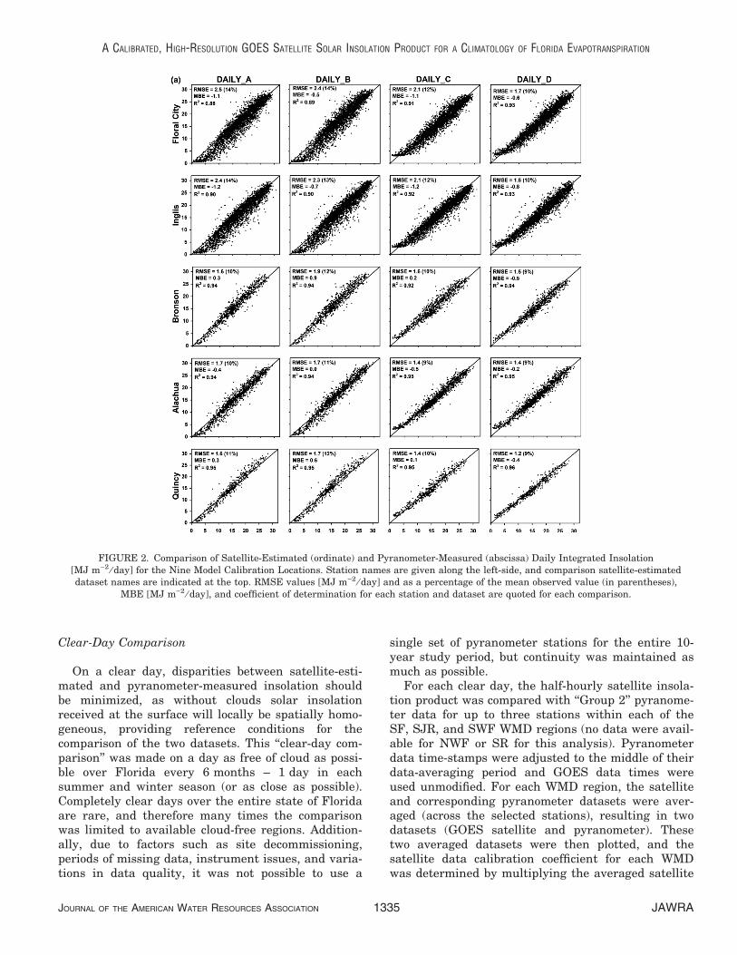
For GDM performance assessment, each of theabove datasets are compared with pyranometer datafrom the ‘‘Group 1’’ dataset, consisting of nine calibra-tion-independent surface stations located across Flor-ida as detailed in Figure 1 and Table 1. The results,showing the calibration progression, are shown forthe entire data period and each of the nine stationlocations in Figure 2. Statistics used for this compari-son (quoted on each plot) are the RMSE (alsoexpressed as a percentage of the mean pyranometer

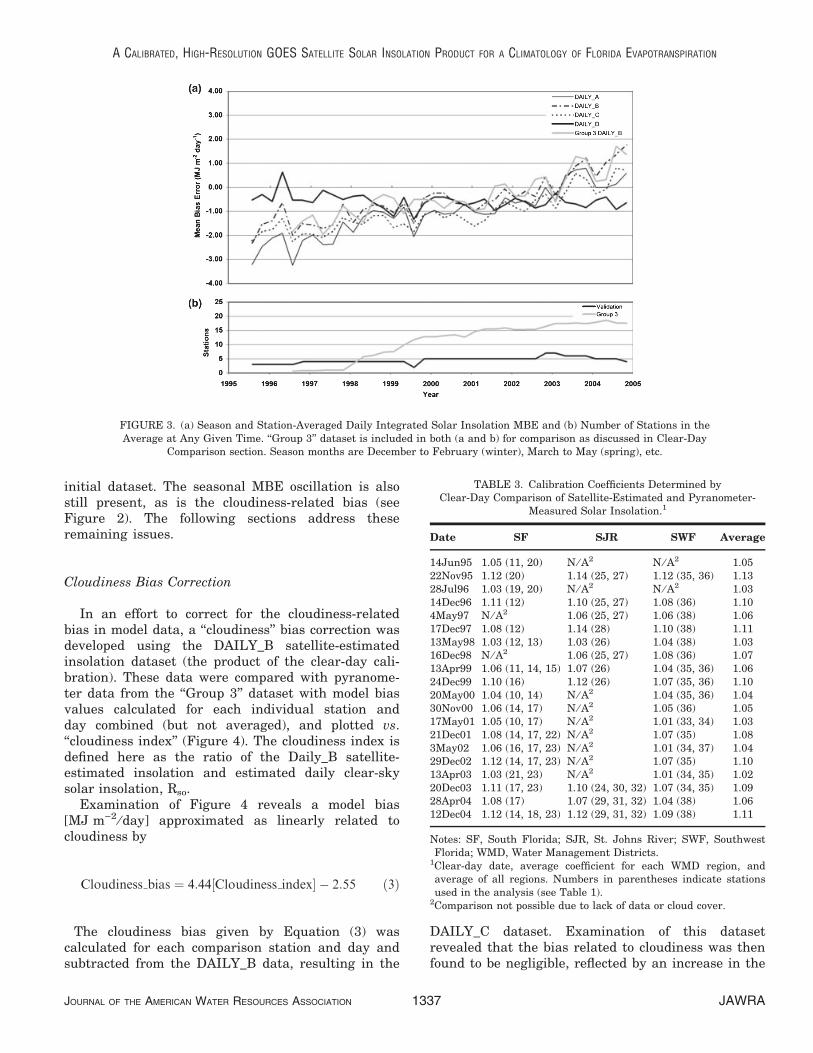
observed value), the mean bias error (MBE), and thecoefficient of determination (R2). Table 2 andFigure 3a present station-averaged statistics and sea-sonal station-averaged model MBE, respectively. Notethat the number of stations in the averaged statistics(Figure 3b) varies from 2 to 7, subject to the datarecord length of each station and the necessity forquality data for comparison. Similar comparisonsusing the half-hourly resolution insolation could notbe made since calibration was only performed for thedaily insolation product.

Initial Results

Station-averaged calibration statistics from theinitial dataset (DAILY_A: Figures 2 and 3 andTable 2) are as follows: coefficient of determination0.90, MBE )0.7 MJ m)2 ⁄ day, and RMSE2.2 MJ m)2 ⁄ day (13% of the mean observed value).These statistics indicates performance slightlypoorer than previous studies using the GDM, whichgenerally had RMSE values of about 10% of themean observed value for daily integrated insolationcomparisons (see the section titled The Solar Insola-tion Model). Figure 3a shows a predominantly nega-tive bias in model-estimated daily insolation values,gradually increasing to a slight positive bias beyondmid-2003, with about a 4 MJ m)2 ⁄ day differencefrom the beginning to the end of the 10-year histor-ical data period. A seasonal bias oscillation on theorder of ±0.5 MJ m)2 ⁄ day is also present, withMBE values tending to be more positive during thesummer and autumn seasons. This trend is clearerin the latter years of the data period (2001onward), with increasing numbers of stations in theaverage (see Figure 3b). Due to the larger numberof stations, this seasonal trend is more evidentwhen comparing with the pyranometer data of the‘‘Group 3’’ dataset (see Section Pyranometer Data) –the station average MBE, which is also plotted inFigure 3a (Group 3 DAILY_B). These observationsare discussed further in the section titled Discus-sion of Calibration Issues.

The scatter plots of Figure 2 reveal an overestima-tion and underestimation of insolation by the GDMunder clear and cloudy conditions, respectively – withthe latter being most prevalent. The occasional datapoint where pyranometer data were significantlyunderestimating insolation is also observed, whichmay be due to the so-called ‘‘bird effect’’ – when birdsuse the pyranometer as a perch and shade the sensor(personal communication with USGS staff). Theapproach we use to fine-tune and correct the data forsome of these observations are described in the fol-lowing sections.



Clear-Day Comparison

On a clear day, disparities between satellite-esti-mated and pyranometer-measured insolation shouldbe minimized, as without clouds solar insolationreceived at the surface will locally be spatially homo-geneous, providing reference conditions for thecomparison of the two datasets. This ‘‘clear-day com-parison’’ was made on a day as free of cloud as possi-ble over Florida every 6 months – 1 day in eachsummer and winter season (or as close as possible).Completely clear days over the entire state of Floridaare rare, and therefore many times the comparisonwas limited to available cloud-free regions. Addition-ally, due to factors such as site decommissioning,periods of missing data, instrument issues, and varia-tions in data quality, it was not possible to use a

single set of pyranometer stations for the entire 10-year study period, but continuity was maintained asmuch as possible.

For each clear day, the half-hourly satellite insola-tion product was compared with ‘‘Group 2’’ pyranome-ter data for up to three stations within each of theSF, SJR, and SWF WMD regions (no data were avail-able for NWF or SR for this analysis). Pyranometerdata time-stamps were adjusted to the middle of theirdata-averaging period and GOES data times wereused unmodified. For each WMD region, the satelliteand corresponding pyranometer datasets were aver-aged (across the selected stations), resulting in twodatasets (GOES satellite and pyranometer). Thesetwo averaged datasets were then plotted, and thesatellite data calibration coefficient for each WMDwas determined by multiplying the averaged satellite

FIGURE 2. Comparison of Satellite-Estimated (ordinate) and Pyranometer-Measured (abscissa) Daily Integrated Insolation[MJ m)2 ⁄ day] for the Nine Model Calibration Locations. Station names are given along the left-side, and comparison satellite-estimateddataset names are indicated at the top. RMSE values [MJ m)2 ⁄ day] and as a percentage of the mean observed value (in parentheses),

MBE [MJ m)2 ⁄ day], and coefficient of determination for each station and dataset are quoted for each comparison.



data by a factor necessary for its diurnal insolationcurve to align with the averaged pyranometer datacurve as closely as possible. This factor was manu-ally determined as a means of correcting for thesatellite-pyranometer differences. Subsequently, theaverage of all available WMD correction factorswere taken to obtain a calibration coefficient forthat particular day for application over the entirestate of Florida. This process was carried out for theentire observation period, resulting in a set of 20approximately biannual calibration coefficients span-ning the 10-year data record, as shown in Table 3.The individual coefficients, obtained only on days

when pyranometer data were available, were theninterpolated in time to obtain a calibration coeffi-cient set that could be applied to each day acrossthe data record.

As a check for potential issues, calibration factorsusing the above method were obtained for 3 consecu-tive clear days (March 6-8, 2001, results not shown inTable 3). During these days weather conditionsremained consistent over Florida, implying that if theapplication of the GDM in this study was successful,the same should be the case of the three calibrationfactors. This was the case: the calibration coefficientof each day had a value of 1.09.

For the model calibration, these coefficients wereapplied to the initial (DAILY_A) data, yielding theDAILY_B dataset. The results of this calibration areshown in Figures 2 and 3 and Table 2. The station-averaged RMSE remained the same as that of theinitial dataset, the coefficient of determinationincreased to 0.91, and the average MBE decreased inmagnitude from )0.7 to )0.2 MJ m)2 ⁄ day (Table 2).Figure 3 reveals that although the MBE has beenreduced on average, the temporal trend of MBE(positive shift with time) is still present, with a sim-ilar range (from dataset beginning to end) as the

FIGURE 2. (Continued)

TABLE 2. Calibration and Comparison Station-AveragedStatistics for Data Period.1

DAILY_A DAILY_B DAILY_C DAILY_D

RMSE MJ m)2 ⁄ day (%) 2.2 (13) 2.2 (13) 1.9 (11) 1.7 (10)MBE MJ m)2 ⁄ day )0.7 )0.2 )0.8 )0.5R2 0.90 0.91 0.92 0.93

Notes: MBE, mean bias error; RMSE, root mean square error.1RMSE as percentage of mean observed value given in parenthe-ses.



initial dataset. The seasonal MBE oscillation is alsostill present, as is the cloudiness-related bias (seeFigure 2). The following sections address theseremaining issues.

Cloudiness Bias Correction

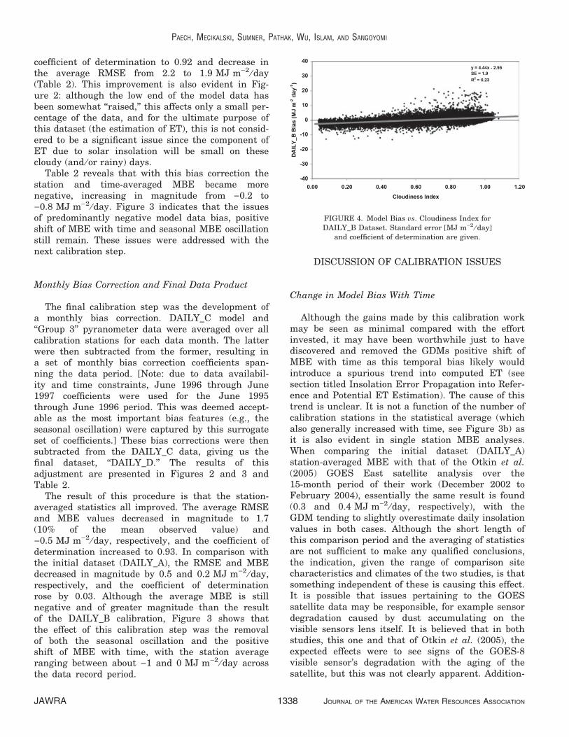
In an effort to correct for the cloudiness-relatedbias in model data, a ‘‘cloudiness’’ bias correction wasdeveloped using the DAILY_B satellite-estimatedinsolation dataset (the product of the clear-day cali-bration). These data were compared with pyranome-ter data from the ‘‘Group 3’’ dataset with model biasvalues calculated for each individual station andday combined (but not averaged), and plotted vs.‘‘cloudiness index’’ (Figure 4). The cloudiness index isdefined here as the ratio of the Daily_B satellite-estimated insolation and estimated daily clear-skysolar insolation, Rso.

Examination of Figure 4 reveals a model bias[MJ m)2 ⁄ day] approximated as linearly related tocloudiness by

Cloudiness bias ¼ 4:44½Cloudiness index� � 2:55 ð3Þ

The cloudiness bias given by Equation (3) wascalculated for each comparison station and day andsubtracted from the DAILY_B data, resulting in the

DAILY_C dataset. Examination of this datasetrevealed that the bias related to cloudiness was thenfound to be negligible, reflected by an increase in the

FIGURE 3. (a) Season and Station-Averaged Daily Integrated Solar Insolation MBE and (b) Number of Stations in theAverage at Any Given Time. ‘‘Group 3’’ dataset is included in both (a and b) for comparison as discussed in Clear-Day

Comparison section. Season months are December to February (winter), March to May (spring), etc.

TABLE 3. Calibration Coefficients Determined byClear-Day Comparison of Satellite-Estimated and Pyranometer-

Measured Solar Insolation.1

Date SF SJR SWF Average

14Jun95 1.05 (11, 20) N ⁄ A2 N ⁄ A2 1.0522Nov95 1.12 (20) 1.14 (25, 27) 1.12 (35, 36) 1.1328Jul96 1.03 (19, 20) N ⁄ A2 N ⁄ A2 1.0314Dec96 1.11 (12) 1.10 (25, 27) 1.08 (36) 1.104May97 N ⁄ A2 1.06 (25, 27) 1.06 (38) 1.0617Dec97 1.08 (12) 1.14 (28) 1.10 (38) 1.1113May98 1.03 (12, 13) 1.03 (26) 1.04 (38) 1.0316Dec98 N ⁄ A2 1.06 (25, 27) 1.08 (36) 1.0713Apr99 1.06 (11, 14, 15) 1.07 (26) 1.04 (35, 36) 1.0624Dec99 1.10 (16) 1.12 (26) 1.07 (35, 36) 1.1020May00 1.04 (10, 14) N ⁄ A2 1.04 (35, 36) 1.0430Nov00 1.06 (14, 17) N ⁄ A2 1.05 (36) 1.0517May01 1.05 (10, 17) N ⁄ A2 1.01 (33, 34) 1.0321Dec01 1.08 (14, 17, 22) N ⁄ A2 1.07 (35) 1.083May02 1.06 (16, 17, 23) N ⁄ A2 1.01 (34, 37) 1.0429Dec02 1.12 (14, 17, 23) N ⁄ A2 1.07 (35) 1.1013Apr03 1.03 (21, 23) N ⁄ A2 1.01 (34, 35) 1.0220Dec03 1.11 (17, 23) 1.10 (24, 30, 32) 1.07 (34, 35) 1.0928Apr04 1.08 (17) 1.07 (29, 31, 32) 1.04 (38) 1.0612Dec04 1.12 (14, 18, 23) 1.12 (29, 31, 32) 1.09 (38) 1.11

Notes: SF, South Florida; SJR, St. Johns River; SWF, SouthwestFlorida; WMD, Water Management Districts.

1Clear-day date, average coefficient for each WMD region, andaverage of all regions. Numbers in parentheses indicate stationsused in the analysis (see Table 1).

2Comparison not possible due to lack of data or cloud cover.



coefficient of determination to 0.92 and decrease inthe average RMSE from 2.2 to 1.9 MJ m)2 ⁄ day(Table 2). This improvement is also evident in Fig-ure 2: although the low end of the model data hasbeen somewhat ‘‘raised,’’ this affects only a small per-centage of the data, and for the ultimate purpose ofthis dataset (the estimation of ET), this is not consid-ered to be a significant issue since the component ofET due to solar insolation will be small on thesecloudy (and ⁄ or rainy) days.

Table 2 reveals that with this bias correction thestation and time-averaged MBE became morenegative, increasing in magnitude from )0.2 to)0.8 MJ m)2 ⁄ day. Figure 3 indicates that the issuesof predominantly negative model data bias, positiveshift of MBE with time and seasonal MBE oscillationstill remain. These issues were addressed with thenext calibration step.

Monthly Bias Correction and Final Data Product

The final calibration step was the development ofa monthly bias correction. DAILY_C model and‘‘Group 3’’ pyranometer data were averaged over allcalibration stations for each data month. The latterwere then subtracted from the former, resulting ina set of monthly bias correction coefficients span-ning the data period. [Note: due to data availabil-ity and time constraints, June 1996 through June1997 coefficients were used for the June 1995through June 1996 period. This was deemed accept-able as the most important bias features (e.g., theseasonal oscillation) were captured by this surrogateset of coefficients.] These bias corrections were thensubtracted from the DAILY_C data, giving us thefinal dataset, ‘‘DAILY_D.’’ The results of thisadjustment are presented in Figures 2 and 3 andTable 2.

The result of this procedure is that the station-averaged statistics all improved. The average RMSEand MBE values decreased in magnitude to 1.7(10% of the mean observed value) and)0.5 MJ m)2 ⁄ day, respectively, and the coefficient ofdetermination increased to 0.93. In comparison withthe initial dataset (DAILY_A), the RMSE and MBEdecreased in magnitude by 0.5 and 0.2 MJ m)2 ⁄ day,respectively, and the coefficient of determinationrose by 0.03. Although the average MBE is stillnegative and of greater magnitude than the resultof the DAILY_B calibration, Figure 3 shows thatthe effect of this calibration step was the removalof both the seasonal oscillation and the positiveshift of MBE with time, with the station averageranging between about )1 and 0 MJ m)2 ⁄ day acrossthe data record period.

DISCUSSION OF CALIBRATION ISSUES

Change in Model Bias With Time

Although the gains made by this calibration workmay be seen as minimal compared with the effortinvested, it may have been worthwhile just to havediscovered and removed the GDMs positive shift ofMBE with time as this temporal bias likely wouldintroduce a spurious trend into computed ET (seesection titled Insolation Error Propagation into Refer-ence and Potential ET Estimation). The cause of thistrend is unclear. It is not a function of the number ofcalibration stations in the statistical average (whichalso generally increased with time, see Figure 3b) asit is also evident in single station MBE analyses.When comparing the initial dataset (DAILY_A)station-averaged MBE with that of the Otkin et al.(2005) GOES East satellite analysis over the15-month period of their work (December 2002 toFebruary 2004), essentially the same result is found(0.3 and 0.4 MJ m)2 ⁄ day, respectively), with theGDM tending to slightly overestimate daily insolationvalues in both cases. Although the short length ofthis comparison period and the averaging of statisticsare not sufficient to make any qualified conclusions,the indication, given the range of comparison sitecharacteristics and climates of the two studies, is thatsomething independent of these is causing this effect.It is possible that issues pertaining to the GOESsatellite data may be responsible, for example sensordegradation caused by dust accumulating on thevisible sensors lens itself. It is believed that in bothstudies, this one and that of Otkin et al. (2005), theexpected effects were to see signs of the GOES-8visible sensor’s degradation with the aging of thesatellite, but this was not clearly apparent. Addition-

FIGURE 4. Model Bias vs. Cloudiness Index forDAILY_B Dataset. Standard error [MJ m)2 ⁄ day]

and coefficient of determination are given.



ally, on April 1, 2003, the GOES-12 satellite took overoperations from the GOES-8 satellite. With the freshsensors on board the new spacecraft, we expected tosee a sudden change in the model data bias, butagain this was not evident in these data. It isbelieved that in both cases, the expected effects arenot clearly seen because they are masked by theinherent limitations of the GDM and this particularapplication of it. Although this issue of satellite sen-sor degradation has not been directly addressed, theeffects of it have been indirectly corrected for throughthe calibration process of this work.

Seasonal Bias Oscillation

With regard to the seasonal oscillation observed inthe model data MBE, both Pinker et al. (2003) andOtkin et al. (2005) observed such an oscillation overthe 1-year to 2-year periods of their analyses, withthe MBE generally being more positive in the sum-mer months. Comparing the initial dataset with theGOES East satellite analysis of Otkin et al. (2005) forthe time period of their work, but now on a seasonalbasis, similar station-averaged MBE values werefound. As for the increase in model bias trend withtime, the reason for this seasonal trend is alsounclear; it is not due to cloudier conditions duringthe Florida summer, as (discussed in the section theCloudiness Bias Correction) the GDM tends to under-estimate rather than overestimate insolation undercloudy conditions. It may simply be due to inherentlimitations of the GDM algorithm, for example sea-sonal sun-angle effects that are not accounted for.Fortunately, and regardless of the cause, this biasoscillation was estimated to be small, even in theinitial dataset.

Comparison With Previous Studies

The RMSE of 10% of the mean observed value forthe final dataset is comparable with the (un-cali-brated) results of previous studies. We believe thismight be because of the complex and prevalent cloudconditions of Florida relative to previous studyareas, leading to a particularly challenging applica-tion of the model. Previous studies have found thatas cloudiness increased GDM performance decreased.Gu et al. (1999) found coefficient of determinationvalues of 0.96, 0.77, and 0.59 for half-hourly obser-vations during clear, partly cloudy, and cloudy condi-tions, respectively, over forested regions of centralCanada. Otkin et al. (2005) found similar results,with lower coefficients of determination and higherRMSE values in the complex cumulus cloud environ-

ments of summer months. The study of Jacobs et al.(2002) over northern-central Florida reported a simi-lar conclusion in comparison with studies over lessconvective-cloud-prone locations and seasons. Resultsfrom the GOES component of the GEWEX SRBproduct (Meng et al., 2003) show that RMSEs arenear 32 Wm)2 for their 0.5� shortwave radiationproduct.

Further Dataset Applications

The data-mining possibilities for such a datasetare vast. As an example, Figure 5 shows the9-year (1996-2004) mean daily solar insolation forthe state of Florida for January 1 and the month ofJanuary. Similarly, Figure 6 shows the 10-year(1995-2004) mean for July 1 and the month of July.(The 10-year average is not available for Januarybecause the dataset begins in June 1995.) Theseimages reveal spatial biases in solar insolationincluding the generally cloudier conditions overland than sea; chronic clear-sky conditions overLake Okeechobee; relatively clear-sky conditions inSWF compared to the cloudier southeast coast inJanuary; and hints of an urban heat island-inducedclear-sky bias in the cities of Orlando and Jackson-ville.

Such data could also serve for applications such asdetailed radiation monitoring to detect climatechange (in the radiation component of climate), andin the resulting impacts on ET. Furthermore, themethod described in this work could be applied toany region in the world for which the appropriatesatellite and pyranometer data are available. Itshould be noted that a full network of pyranometers(as used in this study) is desirable for product cali-bration, yet because this is cost-prohibitive, less than20 instruments distributed across an area such asthe state of Florida would suffice.

Insolation Error Propagation into Reference andPotential ET Estimation

Given that the insolation data, developed here asa long-term climatology, are valuable for determin-ing ET (reference and potential), it is useful to dis-cuss how errors in insolation propagate through toerrors in ET. Analysis of the procedures that relatesolar insolation to potential and reference ET sug-gests that potential ET is perhaps more influencedby errors in insolation because the computationscannot be offset by an aerodynamic component,which is present in the reference ET equations(Dave Sumner-USGS and Jennifer Jacobs-University



of New Hampshire, personal communications). Forexample, it is understood that via the Priestley-Tay-lor approach (Priestley and Taylor, 1972) as used bythe USGS, potential ET is directly proportional tonet radiation, and specifically to the shortwave com-ponent. Also, solar insolation enters into the

longwave calculation of potential ET through atmo-spheric emissivity, which is especially importantduring clear skies, as they produce more negativenet daily longwave radiation. In this light, we esti-mate that a 10% error in insolation causes a 5-6%error in ET is somewhat higher for potential ET.

(a)

(b)

FIGURE 5. The 9-Year (1996-2004) Mean Daily Solar Insolationfor January 1 (a) and the Month of January (b).

(a)

(b)

FIGURE 6. The 10-Year (1995-2004) Mean Daily Solar Insolationfor July 1 (a) and the Month of July (b).



This error will be higher in summer, with morelongwave radiation at this time of year and lowersurface resistances (aerodynamic and soil), than inwinter (USGS, personal communications).

SUMMARY AND CONCLUSION

GOES satellite estimates of incoming solar radia-tion (insolation) for the state of Florida have beenmade using the model of Gautier et al. (1980) (the‘‘GDM’’) for the period June 1995 to December 2004.The dataset has been produced with 2 km spatial,and half-hour and daily temporal resolution. In addi-tion, a 2-week running minimum surface albedo prod-uct was generated, also at 2 km resolution. Throughcomparison with ground-based pyranometer data, aseries of cumulative calibration steps were developedto de-bias and fine-tune the daily integrated insola-tion product.

It was found that the initial (uncalibrated) GDMproduct (DAILY_A) performed well, but slightlypoorer than previous studies, with a calibration sta-tion-averaged value of the coefficient of determinationof 0.90, MBE of )0.7 MJ m)2 ⁄ day, and RMSE of2.2 MJ m)2 ⁄ day (13% of the mean observed value).The model data had a predominantly negative biasthat became increasingly positive with time over thedata record period. A seasonal bias oscillation wasalso discovered, with MBE values tending to be morepositive in the summer and autumn seasons. Addi-tionally, the model was found to overestimate andunderestimate solar insolation under clear and cloudyconditions, respectively, with the latter being mostevident.

Following the three calibration steps, the finalproduct (DAILY_D) showed improvements in compar-ison with the initial dataset, with the station-aver-aged coefficient of determination increasing to 0.93,and MBE and RMSE values decreasing in magnitudeto )0.5 and 1.7 MJ m)2 ⁄ day, respectively. Perhaps,the most significant effect of this calibration effortwas to remove both the positive shift of model biaswith time and the seasonal bias oscillation. The finaldataset RMSE (10% of the mean observed value) iscomparable with the (un-calibrated) results of previ-ous studies. It is believed this may be due to thecloudy conditions of Florida relative to previous studyareas, leading to a particularly challenging applica-tion of the model.

Solar insolation is the largest determinant for tem-poral variation in ET in wet regions, like those oftenfound across the state of Florida (when soil water isnever limiting and the advection of heat is absent),

and hence is a critical variable in water managementefforts. The most desirable ET datasets for these pur-poses are spatially continuous, rather than those withpoint values derived from traditional field station net-works. Thus, mapping of ET over large regions isgreatly facilitated by satellite-derived estimates ofthe spatial distribution of solar insolation. Thisstudy’s final (potential and reference) ET product willbe used in such an effort, by the five Florida WMDs.Work is underway to continue data production (2005to present) and provide ongoing annual datasetupdates.

Additional applications for this dataset are numer-ous, and include via the reference ET field, solarenergy estimation, irrigation scheduling, water allo-cation management, and crop-type planting decisions.Solar insolation to formulate potential ET can beused as input into surface and groundwater hydrolog-ical models (such as the USGS MODFLOW ground-water flow model, MikeShe and HSPF subsurfaceand surface water models), as well as for wildlife andwild-land monitoring. The solar insolation data them-selves may be used as boundary conditions in ecosys-tem modeling and oceanic modeling. Furthermore,the GDM method could be applied to any region inthe world for which the appropriate satellite data(and pyranometer data for calibration) are available,thereby providing such observations for remote, inac-cessible, or hazardous regions, large water bodies, orfor countries that do not have the means to install aground-based observation network.

ACKNOWLEDGMENTS

We would like to thank the following people for their contribu-tions, cooperation, and patience that made this work possible:George Robinson of St. Johns River WMD, Michael Hancock ofSouthwest Florida WMD, and Jennifer Jacobs of the University ofNew Hampshire. We also acknowledge funding support for thisproject from the State of Florida WMD: St. Johns River, SouthFlorida, Southwest Florida, Suwannee River, and Northwest Flor-ida. This work was made possible by U.S. Geological SurveyResearch Grant 05ERAG0027.

LITERATURE CITED

Allen, R.G., 1996. Assessing Integrity of Weather Data for Use inReference Evapotranspiration Estimation. Journal of Irrigationand Drainage Engineering, ASCE 122:97-106.

Allen, R.G., I.A. Walter, R.L. Elliott, T.A. Howell, D. Itenfisu, M.E.Jensen, and R.L. Snyder, 2005. The ASCE Standardized Refer-ence Evapotranspiration Equation. American Society of CivilEngineers, Reston, Virginia.

Anderson, M.C., W.L. Bland, J.M. Norman, and G.R. Diak, 2001.Canopy Wetness and Humidity Prediction Using Satellite andSynoptic-Scale Meteorological Observations. Plant Disease85:1018-1026.



Anderson, M.C., W.P. Kustas, and J.M. Norman, 2003. Upscalingand Downscaling – A Regional View of the Soil-Plant-Atmo-sphere Continuum. Agronomic Journal 95:1408-1432.

Anderson, M.C., J.M. Norman, J.R. Mecikalski, R.D. Torn, W.P.Kustas, and J.B. Basara, 2004. A Multiscale Remote SensingModel for Disaggregating Regional Fluxes to Micrometeorologi-cal Scales. Journal of Hydrometeorology 5:343-363.

Cosgrove, Brian A., Dag Lohmann, Kenneth E. Mitchell, Paul R.Houser, Eric F. Wood, John Schaake, Alan Robock, CurtisMarshall, Justin Sheffield, Lifeng Luo, Qingyun Duan, RachelT. Pinker, J. Dan Tarpley, R. Wayne Higgins, and Jesse Meng,2003a. Realtime and Retrospective Forcing in the North Ameri-can Land Data Assimilation Systems (NLDAS) Project. Journalof Geophysical Research 108(D22):8842, doi: 10.1029/2002JD003118.

Cosgrove, Brian A., Dag Lohmann, Kenneth E. Mitchell, Paul R.Houser, Eric F. Wood, John C. Schaake, Alan Robock, JustinSheffield, Qingyun Duan, Lifeng Luo, R. Wayne Higgins, RachelT. Pinker, and J. Dan Tarpley, 2003b. Land Surface Model Spin-up Behavior in the North American Land Data AssimilationSystem (NLDAS). Journal of Geophysical Research 108(D22):8845, doi: 10.1029/2002JD003119.

Darnell, W.L., W.F. Staylor, S.K. Gupta, and F.M. Denn, 1988.Estimation of Surface Insolation Using Sun-Synchronous Satel-lite Data. Journal of Climate 1:820-835.

Dedieu, G., P.Y. Deschamps, and Y.H. Kerr, 1987. Satellite Esti-mates of Solar Irradiance at the Surface of the Earth and ofSurface Albedo Using a Physical Model Applied to MeteosatData. Journal of Climate and Applied Meteorology 26:79-87.

Diak, G.R., M.C. Anderson, W.L. Bland, J.M. Norman, J.R. Meci-kalski, and R.M. Aune, 1998. Agricultural Management Deci-sions Aids Driven by Real-Time Satellite Data. Bulletin ofAmerican Meteorological Society 79:1345-1355.

Diak, G.R., W.L. Bland, and J.R. Mecikalski, 1996. A Note on FirstEstimates of Surface Insolation From GOES-8 Visible SatelliteData. Agricultural and Forest Meteorology 82:219-226.

Diak, G.R. and C. Gautier, 1983. Improvements to a Simple Physi-cal Model for Estimating Insolation From GOES Data. Journalof Climate and Applied Meteorology 22:505-508.

Duffie, J.A. and W.A. Beckman, 1980. Solar Engineering of Ther-mal Processes. John Wiley and Sons, New York, pp. 1-109.

Frouin, R. and B. Chertock, 1992. A Technique for Global Monitor-ing of net Solar Irradiance at the Ocean Surface. Part I: Model.Journal of Applied Metrology 31:1056-1066.

Frouin, R., C. Gautier, K.B. Katsaros, and J. Lind, 1988. A Com-parison of Satellite and Empirical Formula Techniques for Esti-mating Insolation Over the Oceans. Journal of AppliedMetrology 27:1016-1023.

Gautier, C., G.R. Diak, and S. Masse, 1980. A Simple Physical Modelto Estimate Incident Solar Radiation at the Surface From GOESSatellite Data. Journal of Applied Metrology 19:1007-1012.

Gautier, C., G.R. Diak, and S. Masse, 1984. An Investigation of theEffects of Spatially Averaging Satellite Brightness Measure-ments on the Calculation of Insolation. Journal of Climate andApplied Meteorology 23:1380-1386.

Gu, J., E.A. Smith, and J.D. Merritt, 1999. Testing Energy BalanceClosure With GOES-Retrieved Net Radiation and In Situ Mea-sured Eddy Correlation Fluxes in BOREAS. Journal of Geophys-ical Research 104:27881-27893.

Hoblit, B.C., C. Castello, L. Liu, and D. Curtis, 2003. Creating a Seam-less Map of Gage-Adjusted Radar Rainfall Estimates for the Stateof Florida. Paper presented at EWRI World Water and Environ-mental Congress, Philadelphia, Pennsylvania, 23-26 June.

Jacobs, J.M., M.C. Anderson, L.C. Friess, and G.R. Diak, 2004.Solar Radiation, Longwave Radiation and Emergent WetlandEvapotranspiration Estimates From Satellite Data in Florida,USA. Hydrological Sciences Journal 49:461-476.

Jacobs, J.M., D.A. Myers, M.C. Anderson, and G.R. Diak, 2002.GOES Surface Insolation to Estimate Wetlands Evapotranspira-tion. Journal of Hydrology 56:53-65.

Mecikalski, J.M., G.R. Diak, M.C. Anderson, and J.M. Norman,1999. Estimating Fluxes on Continental Scales Using RemotelySensed Data in an Atmosphere-Land Exchange Model. Journalof Applied Metrology 38:1352-1369.

Meng, C. Jesse, Rachel T. Pinker, J. Dan Tarpley, and Istvan Las-zlo, 2003. A Satellite Approach for Estimating Regional LandSurface Energy Budget for GCIP ⁄ GAPP. Journal of GeophysicalResearch 108(D22):8861, doi: 10.1029/2002JD003088.

Monteith, J.L., 1965. Evaporation and Environment. Symposia ofthe Society for Experimental Biology 19:205-224.

Moser, W. and E. Raschke, 1984. Incident Solar Radiation OverEurope From METEOSAT Data. Journal of Climate andApplied Meteorology 23:166-170.

Otkin, J., M.A. Anderson, J.R. Mecikalski, and G.R. Diak, 2005.Validation of GOES-Based Insolation Estimates Using DataFrom the United States Climate Reference Network. Journal ofHydrometeorology 6:475-640.

Penman, H.L., 1948. Natural Evaporation From Open Water, BareSoil and Grass. Proceedings of Royal Society London A 194, S.120-145.

Pinker, R.T. and J.A. Ewing, 1985. Modeling Surface Solar Radia-tion: Model Formulation and Validation. Journal of Climate andApplied Meteorology 24:389-401.

Pinker, R.T., R. Frouin, and Z. Li, 1995. A Review of SatelliteMethods to Derive Surface Shortwave Irradiance. Remote Sens-ing Environment 51:105-124.

Pinker, R.T. and I. Laszlo, 1992. Modeling Surface Solar Irradiancefor Satellite Applications on Global Scale. Journal of AppliedMetrology 31:194-211.

Pinker, R.T., J.D. Tarpley, I. Laszlo, K.E. Mitchell, P.R. Houser,E.F. Wood, J.C. Schaake, A. Robock, D. Lohmann, B.A. Cos-grove, J. Sheffield, Q. Duan, L. Luo, and R.W. Higgins, 2003.Surface Radiation Budgets in Support of the GEWEX Continen-tal-Scale International Project (GCIP) and the GEWEXAmericas Prediction Project (GAPP), Including the NorthAmerican Land Data Assimilation System (NLDAS) Project.Journal of Geophysical Research 108(22):8798, doi: 10.1029/2002JDO03301.

Priestley, C.H.B. and R.J. Taylor, 1972. On the Assessment of Sur-face Heat Flux and Evaporation Using Large-Scale Parameters.Monthly Weather Review 100:81-92.

Raphael, C. and J.E. Hay, 1984. An Assessment of Models WhichUse Satellite Data to Estimate Solar Irradiance at the Earth’sSurface. Journal of Climate and Applied Meteorology 23:832-844.

Schmetz, J., 1989. Towards a Surface Radiation Climatology.Retrieval of Downward Irradiance From Satellites. AtmosphericResearch 23:287-321.

Stewart, J.B., C.J. Watts, J.C. Rodriguez, H.A.R. De Bruin, A.R.van den Berg, and J. Garatuza-Payan, 1999. Use of SatelliteData to Estimate Radiation and Evaporation for NorthwestMexico. Agriculture and Water Management 38:181-193.

Tarpley, J.D., 1979. Estimating Incident Solar Radiation at theSurface From Geostationary Satellite Data. Journal of AppliedMeteorology 18:1172-1181.

Weymouth, G. and J. LeMarshall, 1999. An Operational System toEstimate Global Solar Exposure Over the Australian RegionFrom Satellite Observations. Australian Meteorological Maga-zine 48:181-195.



Documents

A CALIBRATED, HIGH-RESOLUTION GOES SATELLITE SOLAR INSOLATION