Embed Size (px)
Citation preview
A Calculus of Evolving Objects
Mariangiola Dezani-Ciancaglini1, Paola Giannini2 and Oscar Nierstrasz3
1 Dipartimento di Informatica, Univ. di Torino, Italy — www.di.unito.it2 Dipartimento di Informatica, Univ. del Piemonte Orientale, Italy —
www.di.unipmn.it3 Software Composition Group, University of Bern, Switzerland — scg.unibe.ch
Abstract. The demands of developing modern, highly dynamic appli-cations have led to an increasing interest in dynamic programming lan-guages and mechanisms. Not only applications must evolve over time,but the object models themselves may need to be adapted to the require-ments of different run-time contexts. Class-based models and prototype-based models, for example, may need to co-exist to meet the demandsof dynamically evolving applications. Multi-dimensional dispatch, fine-grained and dynamic software composition, and run-time evolution ofbehaviour are further examples of diverse mechanisms which may needto co-exist in a dynamically evolving run-time environment. How can wemodel the semantics of these highly dynamic features, yet still offer somereasonable safety guarantees?To this end we present an original calculus in which objects can adapttheir behaviour at run-time. Both objects and environments are rep-resented by first-class mappings between variables and values. Messagesends are dynamically resolved to method calls. Variables may be dynam-ically bound, making it possible to model a variety of dynamic mecha-nisms within the same calculus. Despite the highly dynamic nature ofthe calculus, safety properties are assured by a type assignment system.
1 Introduction
There has been a recent re-emergence of interest in dynamic programming lan-guages [19] and the development of more dynamic features for mainstream lan-guages such as Java. Increasing numbers of applications require the ability forconfigurations and even system behaviour to evolve at run-time. Furthermore,behaviour may be context-dependent, and may need to adapt to the run-timeplatform, the end user, service availability, or any number of environmental at-tributes. To support these highly dynamic applications, programming languagesneed to support a range of different object models, paradigms and languagefeatures.
Multi-dimensional dispatch is one example of a such a feature — instead ofdispatching purely on the receiver of a message, the behavior of an object mightdepend on the sender, or even on contextual information such as the deploy-ment platform, available services, desired quality of service, available versions ofcomponents, or even the time of day [13]. Another example is the use of fine-grained components, such as traits, to statically or even dynamically extend the
2 M. Dezani, P. Giannini and O. Nierstrasz
behaviour of classes [7]. These and other mechanisms entail the need for spe-cialized lookup mechanisms to adapt the behaviour of objects, even at run-time[22].
It is unclear what the impact of such dynamic features may be on the seman-tics of programming languages, and on the ability to reason about type safety inthe face of dynamic changes. To this end we have developed a stateful calculusof evolving objects in which:
– Object behaviour is context-dependent — message-dispatching takes contextinto account.
– Objects may change their behaviour at run-time — message-lookup may bedynamically updated.
– Dynamic changes are type-safe — message-not-understood errors are avoided.
Particular innovations of the calculus include:
– The use of first-class environments to model both the object states and theenvironments in which expressions are evaluated.
– The possibility of binding dynamically variables by freezing expressions con-taining free variables and defrosting them in a runtime environment provid-ing binders for them.
– Distinguishing message sends from method calls to support object-specific(context-dependent) method lookup.
– A novel type system which— in addition to safety properties — assures thatvariables in an evolving environment are bound to values of fixed types.
The paper is organized as follows. In Section 2 we introduce the calculus throughan example. The syntax and the operational semantics of the language are intro-duced in Sections 3.1 and 3.2. In particular, Section 3.1 introduces the lambda-calculus of environments that is the core functional part of our calculus and inSection 3.2 we add imperative extensible objects in which message send is notidentified with method call. In Section 4 we present an overview of the typesystem with the relevant results. In Section 5 we place our work in context andcontrast it to other approaches. We conclude in Section 6 with some remarks oncurrent and future work. The Appendix contains proofs.
2 An example
In this section we introduce the relevant constructs of our calculus via an ex-ample. The calculus extends the lambda-calculus with explicit substitution andmodels both execution environments and object fields as sequences of bindingsbetween variables and values, x1=V1· · · ·xn=Vn, denoted by the metavariableE. Objects are imperative and their associated environments are allocated inmemory.
Suppose we want to model a Call Centre answering calls. If a request (call)arrives from a client, then the request is sent to the Office with the client identifier
A Calculus of Evolving Objects 3
(a number). Otherwise the Call Centre gives a default answer, e.g., asking toregister to obtain a client number. The way the request is handled thereforedepends on the sender.
We represent the Call Centre by an object, and the request by sending themessage m. Instead of being associated to a field of the object of name m, themethod corresponding to m is dynamically looked up, with a lookup function forthe Call Centre, that uses the message name, the information on the context ofthe sender, and the identity of the sender.
In writing the lookup function we must be able to manipulate message names,and discriminate the execution of expressions according to the fact that thesenames are/are not bound (defined) in the environment representing the object.To this end we distinguish two different ways to evaluate an expression A in anenvironment.
– The first is the sandbox expression E;A, in which the free variables of the ex-pression A must be statically bound to variables defined in the environmentE.
– The second is a conditional expression E◦〈A〉�B to handle the situationwhere the free variables of A might not all be captured by E. If they are, theconditional reduces to E;A as above, otherwise it reduces to the expressionB (similar to a try/catch block for exceptions).
In order to model the second alternative, we introduce the construct 〈A〉. Thisfreezes the expression A, turning it into a closed value even if A contains freevariables. In particular given a (free) message name m, 〈m〉 is a value (whereasm would not be). A frozen expression can be evaluated (defrosted) only in anenvironment that defines all its free variables. As said before, the expressionE◦〈A〉�B— in case all the free variables of A are defined in E— reduces toE;A, thereby dynamically binding the free variables of A to the environment E.If E does not define all the free variable of A the evaluation of the expressionE◦〈A〉�B reduces to B.
Lookup functions, in addition to the name of the message, take into accountthe sender. The sender is determined at run-time. In our calculus we provideboth a user syntax and a run-time syntax for message sends. The user writesA m(B), to send message m to the object denoted by A with B as argument.At run-time the actual message send will be EyA m(B), where E provides con-textual information concerning the message sender extracted from the executionenvironment.
Going back to the Call Centre example, we can assume that the requestarrives from an object, whose contextual information, E, in case the sender isa client, contains a binding, client=N , for the name client to the numberidentifying the sender, otherwise it does not. If ι is the reference to the CallCentre (and in general for any reference), with ∗ι we denote the environmentassociated with ι. Assuming that offExpr is the body that should be evaluatedwhen the request comes from a client, the behaviour of the Call Centre answering
4 M. Dezani, P. Giannini and O. Nierstrasz
one call can be realized by the expression
E◦〈offExpr client 〈request〉〉�(∗ι; defResp)
That is, we evaluate the expression:
offExpr client 〈request〉
if the environment E defines binding for its free variables. In this case, assumingthat offExpr is a close expression the only free variable is client since 〈request〉is a closed expression. Therefore, if E contains client=N the expression reducesto offExpr N 〈request〉. If E does not have a binding for client the value ofthe field defResp of the Call Centre is returned. Field selection is obtainedby evaluating the field name in the sandbox of the object containing the field:∗ι; defResp. If we assume that offExpr is a function associated with the fieldserveReq of the Call Centre object, then offExpr = ∗ι; serveReq.
3 Syntax and Operational Semantics
3.1 First-class environments
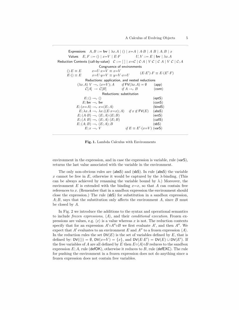
The functional core of our calculus is a Call-By-Value lambda-calculus manip-ulating environments (sets of bindings between names and values). We first in-troduce syntax and operational semantics of the statically scoped section of thecalculus which is a standard lambda-calculus with explicit substitution. We thenintroduce the constructs related to freezing/defrosting expressions.
The syntax and operational semantics for the calculus are given in Fig. 1.The expressions of the calculus, A, B, . . ., in addition to basic values, bv, whichmodel integers, floats etc., and functions λx.A, include bindings, that are asso-ciations between names and expressions built from the empty environment, (),or a binding, x=A using extension, A·B. The binding x=A defines x. ExtensionA·B models environment evolution: the binding x=B′ in B overrides a bindingfor x in A. This is expressed by the congruence on environments, ≡.
Free variables are defined in the standard way. (The free variables of a bindingx=A are the free variables of A.)
The sandbox expression A;B evaluates B within the environment defined byA. Note that this implies that all the free variables of B must be defined in A,or the evaluation will lead to an error. The expression x is the lookup of x inthe environment. Therefore, ();x is an erroneous term since x is not bound inthe environment ().
The operational semantics of this fragment of calculus is given by the relationbetween expressions, A→ B, which is defined by giving the computational steps,→r, and the reduction contexts that determine where they may happen. Thereare two kinds of computational steps: the evaluation of an application, (λx.A) Vwhich reduces to evaluate A in the environment in which x is bound to thevalue V , and the evaluation of an expression in an environment, that pushes the
A Calculus of Evolving Objects 5
Expressions A,B ::= bv | λx.A | () | x=A | A·B | A B | A;B | xValues E,F ::= () | x=V | E·F U, V ::= E | bv | λx.A
Reduction Contexts (call-by-value) C ::= [ ] | x=C | C·A | V ·C | C A | V C | C;A
Congruence of environments()·E ≡ EE·() ≡ E
x=U ·x=V ≡ x=Vx=U ·y=V ≡ y=V ·x=U (E·E′)·F ≡ E·(E′·F )
Reductions: application, and nested reductions(λx.A) V →r (x=V );A if FV(λx.A) = ∅ (app)
C[A] → C[B] if A→r B (cont)
Reductions: substitutionE; () →r () (eptS)E;bv →r bv (conS)
E; (x=A) →r x=(E;A) (bindS)E;λx.A →r λx.((E·x=x);A) if x 6∈ FV(E) (absS)E; (A·B) →r (E;A)·(E;B) (extS)E; (A B) →r (E;A) (E;B) (callS)E; (A;B) →r (E;A);B (sbS)
E;x →r V if E ≡ E′·(x=V ) (varS)
Fig. 1. Lambda Calculus with Environments
environment in the expression, and in case the expression is variable, rule (varS),returns the last value associated with the variable in the environment.
The only non-obvious rules are (absS) and (sbS). In rule (absS) the variablex cannot be free in E, otherwise it would be captured by the λ-binding. (Thiscan be always achieved by renaming the variable bound by λ.) Moreover, theenvironment E is extended with the binding x=x, so that A can contain freereferences to x. (Remember that in a sandbox expression the environment shouldclose the expression.) The rule (sbS) for substitution in a sandbox expression,A;B, says that the substitution only affects the environment A, since B mustbe closed by A.
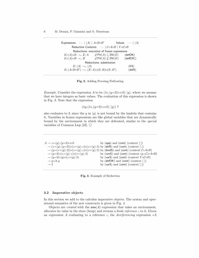
In Fig. 2 we introduce the additions to the syntax and operational semanticsto include frozen expressions, 〈A〉, and their conditional execution. Frozen ex-pressions are values, e.g. 〈x〉 is a value whereas x is not. The reduction contextsspecify that for an expression A′◦A′′�B we first evaluate A′, and then A′′. Weexpect that A′ evaluates to an environment E and A′′ to a frozen expression 〈A〉.In the reduction rules the set DV(E) is the set of variables defined by E, that isdefined by: DV(()) = ∅, DV(x=V ) = {x}, and DV(E·E′) = DV(E) ∪ DV(E′). Ifthe free variables of A are all defined by E then E◦〈A〉�B reduces to the sandboxexpression E;A, rule (defOK), otherwise it reduces to B, rule (defEXC). The rulefor pushing the environment in a frozen expression does not do anything since afrozen expression does not contain free variables.
6 M. Dezani, P. Giannini and O. Nierstrasz
Expressions · · · | 〈A〉 | A◦B�B′ Values · · · | 〈A〉Reduction Contexts · · · | C◦A�B | V ◦C�BReductions: execution of frozen expressions
E◦〈A〉�B →r E;A if FV(A) ⊆ DV(E) (defOK)E◦〈A〉�B →r B if FV(A) 6⊆ DV(E) (defEXC)
Reductions: substitutionE; 〈A〉 →r 〈A〉 (frS)
E; (A◦B�B′) →r (E;A)◦(E;B)�(E;B′) (defS)
Fig. 2. Adding Freezing/Defrosting
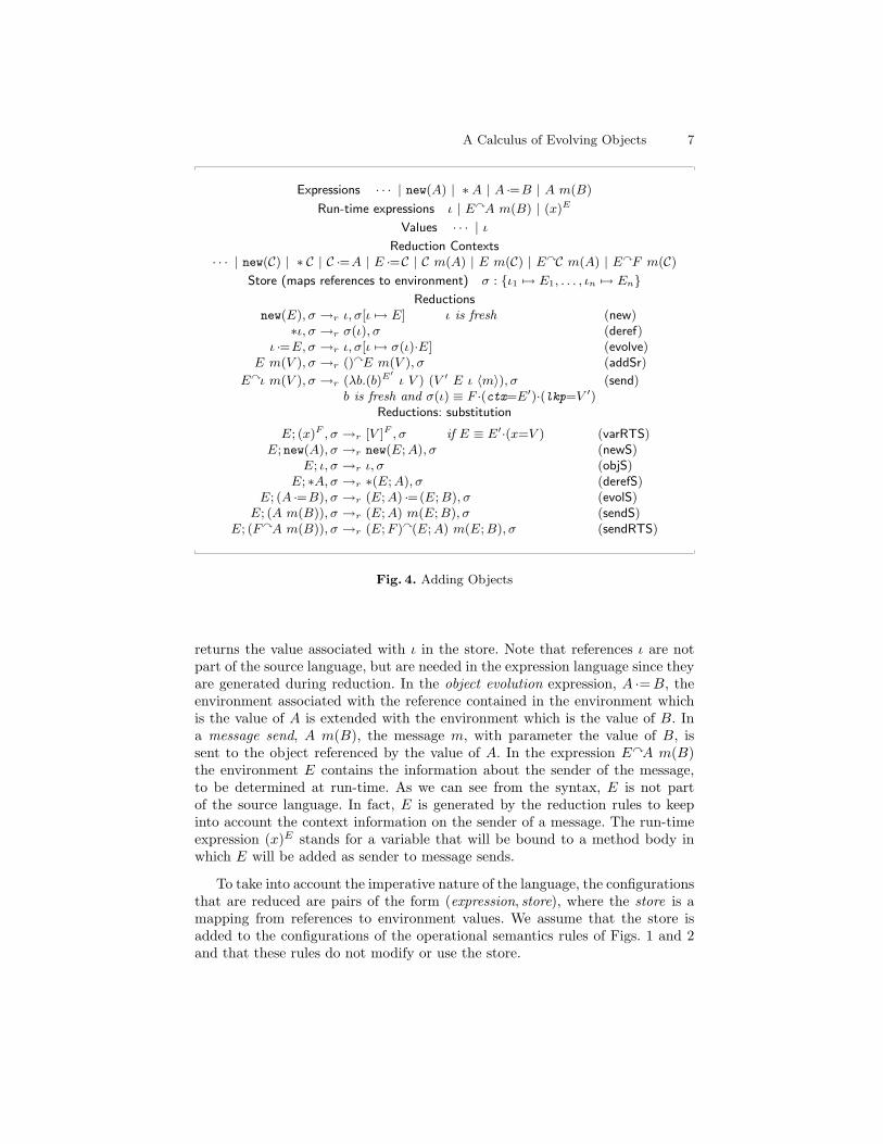
Example. Consider the expression A to be (λz.(y=3)◦z�5) 〈y〉, where we assumethat we have integers as basic values. The evaluation of this expression is shownin Fig. 3. Note that the expression
(λy.(λz.(y=3)◦z�5) 〈y〉) 7
also evaluates to 3, since the y in 〈y〉 is not bound by the lambda that containsit. Variables in frozen expressions are like global variables that are dynamicallybound by the environment in which they are defrosted, similar to the specialvariables of Common Lisp [23]. �
A → z=〈y〉; (y=3)◦z�5 by (app) and (cont) (context [ ])→ (z=〈y〉; (y=3))◦(z=〈y〉; z)�(z=〈y〉; 5) by (defS) and (cont) (context [ ])→ (y=(z=〈y〉; 3))◦(z=〈y〉; z)�(z=〈y〉; 5) by (bindS) and (cont) (context C◦A�B)→ (y=3)◦(z=〈y〉; z)�(z=〈y〉; 5) by (conS) and (cont) (context (y=C)◦A�B)→ (y=3)◦〈y〉�(z=〈y〉; 5) by (varS) and (cont) (context V ◦C�B)→ y=3; y by (defOK) and (cont) (context [ ])→ 3 by (varS) and (cont) (context [ ])
Fig. 3. Example of Reduction
3.2 Imperative objects
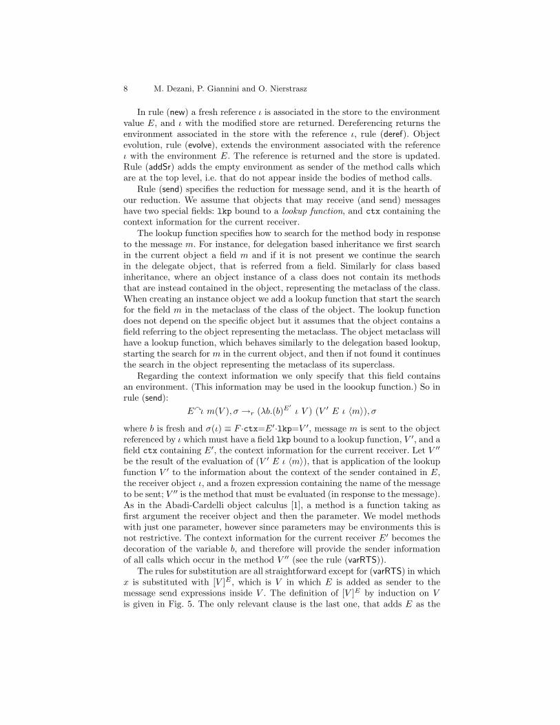
In this section we add to the calculus imperative objects. The syntax and oper-ational semantics of the new constructs is given in Fig. 4.
Objects are created with the new(A) expression that takes an environment,allocates its value in the store (heap) and returns a fresh reference ι to it. Givenan expression A evaluating to a reference ι, the dereferencing expression ∗A
A Calculus of Evolving Objects 7
Expressions · · · | new(A) | ∗A | A ·=B | A m(B)
Run-time expressions ι | EyA m(B) | (x)E
Values · · · | ιReduction Contexts
· · · | new(C) | ∗ C | C ·=A | E ·=C | C m(A) | E m(C) | EyC m(A) | EyF m(C)
Store (maps references to environment) σ : {ι1 7→ E1, . . . , ιn 7→ En}Reductions
new(E), σ →r ι, σ[ι 7→ E] ι is fresh (new)∗ι, σ →r σ(ι), σ (deref)
ι ·=E, σ →r ι, σ[ι 7→ σ(ι)·E] (evolve)E m(V ), σ →r ()yE m(V ), σ (addSr)
Eyι m(V ), σ →r (λb.(b)E′ι V ) (V ′ E ι 〈m〉), σ (send)
b is fresh and σ(ι) ≡ F ·(ctx=E′)·(lkp=V ′)Reductions: substitution
E; (x)F , σ →r [V ]F , σ if E ≡ E′·(x=V ) (varRTS)E; new(A), σ →r new(E;A), σ (newS)
E; ι, σ →r ι, σ (objS)E; ∗A, σ →r ∗(E;A), σ (derefS)
E; (A ·=B), σ →r (E;A) ·=(E;B), σ (evolS)E; (A m(B)), σ →r (E;A) m(E;B), σ (sendS)
E; (FyA m(B)), σ →r (E;F )y(E;A) m(E;B), σ (sendRTS)
Fig. 4. Adding Objects
returns the value associated with ι in the store. Note that references ι are notpart of the source language, but are needed in the expression language since theyare generated during reduction. In the object evolution expression, A ·=B, theenvironment associated with the reference contained in the environment whichis the value of A is extended with the environment which is the value of B. Ina message send, A m(B), the message m, with parameter the value of B, issent to the object referenced by the value of A. In the expression EyA m(B)the environment E contains the information about the sender of the message,to be determined at run-time. As we can see from the syntax, E is not partof the source language. In fact, E is generated by the reduction rules to keepinto account the context information on the sender of a message. The run-timeexpression (x)E stands for a variable that will be bound to a method body inwhich E will be added as sender to message sends.
To take into account the imperative nature of the language, the configurationsthat are reduced are pairs of the form (expression, store), where the store is amapping from references to environment values. We assume that the store isadded to the configurations of the operational semantics rules of Figs. 1 and 2and that these rules do not modify or use the store.
8 M. Dezani, P. Giannini and O. Nierstrasz
In rule (new) a fresh reference ι is associated in the store to the environmentvalue E, and ι with the modified store are returned. Dereferencing returns theenvironment associated in the store with the reference ι, rule (deref). Objectevolution, rule (evolve), extends the environment associated with the referenceι with the environment E. The reference is returned and the store is updated.Rule (addSr) adds the empty environment as sender of the method calls whichare at the top level, i.e. that do not appear inside the bodies of method calls.
Rule (send) specifies the reduction for message send, and it is the hearth ofour reduction. We assume that objects that may receive (and send) messageshave two special fields: lkp bound to a lookup function, and ctx containing thecontext information for the current receiver.
The lookup function specifies how to search for the method body in responseto the message m. For instance, for delegation based inheritance we first searchin the current object a field m and if it is not present we continue the searchin the delegate object, that is referred from a field. Similarly for class basedinheritance, where an object instance of a class does not contain its methodsthat are instead contained in the object, representing the metaclass of the class.When creating an instance object we add a lookup function that start the searchfor the field m in the metaclass of the class of the object. The lookup functiondoes not depend on the specific object but it assumes that the object contains afield referring to the object representing the metaclass. The object metaclass willhave a lookup function, which behaves similarly to the delegation based lookup,starting the search for m in the current object, and then if not found it continuesthe search in the object representing the metaclass of its superclass.
Regarding the context information we only specify that this field containsan environment. (This information may be used in the loookup function.) So inrule (send):
Eyι m(V ), σ →r (λb.(b)E′ι V ) (V ′ E ι 〈m〉), σ
where b is fresh and σ(ι) ≡ F ·ctx=E′·lkp=V ′, message m is sent to the objectreferenced by ι which must have a field lkp bound to a lookup function, V ′, and afield ctx containing E′, the context information for the current receiver. Let V ′′
be the result of the evaluation of (V ′ E ι 〈m〉), that is application of the lookupfunction V ′ to the information about the context of the sender contained in E,the receiver object ι, and a frozen expression containing the name of the messageto be sent; V ′′ is the method that must be evaluated (in response to the message).As in the Abadi-Cardelli object calculus [1], a method is a function taking asfirst argument the receiver object and then the parameter. We model methodswith just one parameter, however since parameters may be environments this isnot restrictive. The context information for the current receiver E′ becomes thedecoration of the variable b, and therefore will provide the sender informationof all calls which occur in the method V ′′ (see the rule (varRTS)).
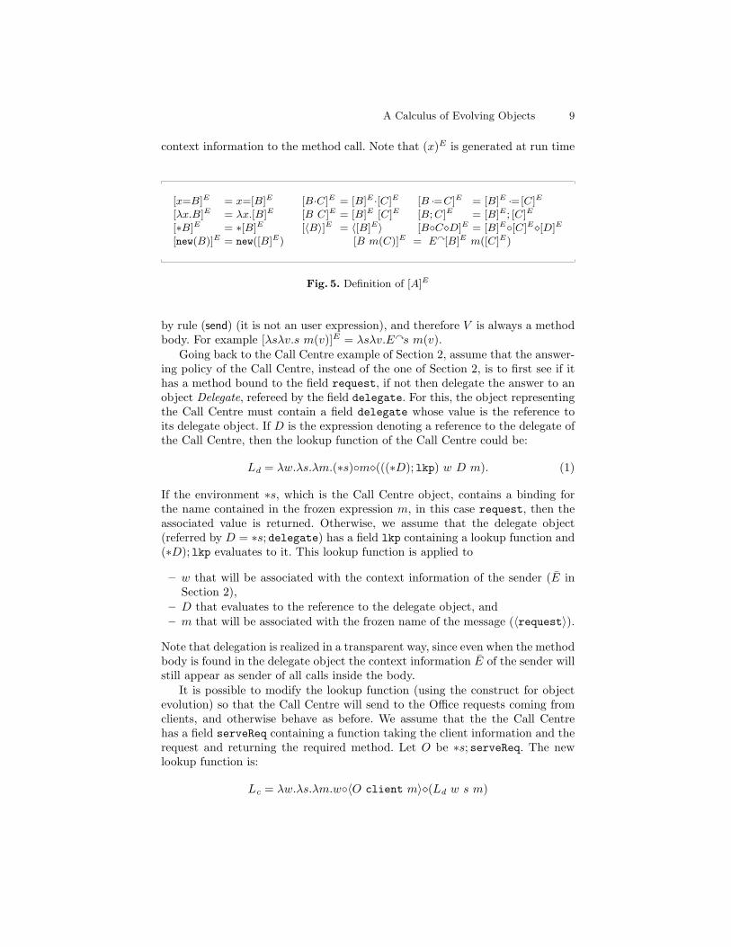
The rules for substitution are all straightforward except for (varRTS) in whichx is substituted with [V ]E , which is V in which E is added as sender to themessage send expressions inside V . The definition of [V ]E by induction on Vis given in Fig. 5. The only relevant clause is the last one, that adds E as the
A Calculus of Evolving Objects 9
context information to the method call. Note that (x)E is generated at run time
[x=B]E = x=[B]E [B·C]E = [B]E ·[C]E [B ·=C]E = [B]E ·=[C]E
[λx.B]E = λx.[B]E [B C]E = [B]E [C]E [B;C]E = [B]E ; [C]E
[∗B]E = ∗[B]E [〈B〉]E = 〈[B]E〉 [B◦C�D]E = [B]E◦[C]E�[D]E
[new(B)]E = new([B]E) [B m(C)]E = Ey[B]E m([C]E)
Fig. 5. Definition of [A]E
by rule (send) (it is not an user expression), and therefore V is always a methodbody. For example [λsλv.s m(v)]E = λsλv.Eys m(v).
Going back to the Call Centre example of Section 2, assume that the answer-ing policy of the Call Centre, instead of the one of Section 2, is to first see if ithas a method bound to the field request, if not then delegate the answer to anobject Delegate, refereed by the field delegate. For this, the object representingthe Call Centre must contain a field delegate whose value is the reference toits delegate object. If D is the expression denoting a reference to the delegate ofthe Call Centre, then the lookup function of the Call Centre could be:
Ld = λw.λs.λm.(∗s)◦m�(((∗D); lkp) w D m). (1)
If the environment ∗s, which is the Call Centre object, contains a binding forthe name contained in the frozen expression m, in this case request, then theassociated value is returned. Otherwise, we assume that the delegate object(referred by D = ∗s; delegate) has a field lkp containing a lookup function and(∗D); lkp evaluates to it. This lookup function is applied to
– w that will be associated with the context information of the sender (E inSection 2),
– D that evaluates to the reference to the delegate object, and– m that will be associated with the frozen name of the message (〈request〉).
Note that delegation is realized in a transparent way, since even when the methodbody is found in the delegate object the context information E of the sender willstill appear as sender of all calls inside the body.
It is possible to modify the lookup function (using the construct for objectevolution) so that the Call Centre will send to the Office requests coming fromclients, and otherwise behave as before. We assume that the the Call Centrehas a field serveReq containing a function taking the client information and therequest and returning the required method. Let O be ∗s; serveReq. The newlookup function is:
Lc = λw.λs.λm.w◦〈O client m〉�(Ld w s m)
10 M. Dezani, P. Giannini and O. Nierstrasz
In Lc the context information on the sender w is used as environment in thedynamic binding. Therefore, if the environment associated with w (the contextinformation on the sender) contains a binding for client, then the request issent to the Office along with the value of the field client. Otherwise, the lookupdefined in (1) is applied. Similarly one can easily write lookup functions whichimplement class-based and trait-based searches of method bodies.
4 Type Assignment System
4.1 Types
In this section we introduce a type system for our calculus. As usual [21] (Sub-section 8.1), the shapes of types are suggested by the shapes of values. We havebasic types for basic values, arrow types for λ-abstractions, reference types forobject references.
The standard typing of a binding x = V is xψ, where ψ is the type of V [21](Subsection 11.8). Since we are interested in expressing that a variable shouldbe bound only to values of a fixed type, also in absence of a binding, we allowbinding types of the shape x†ψ, where † ∈ {!, ?}. The meaning of x!ψ is that x isactually bound to a value of type ψ, while x?ψ says that x can only be boundto a value of type ψ. We say that x is the subject and ψ is the predicate of x†ψ.The type of an environment is a set of binding types with different subjects. Theempty environment is naturally typed by the empty set.
A frozen expression requires its set of free variables to be bound with valuesof fixed types: for this reason we type a frozen expression with a pair 〈Γ, ψ〉(frozen type), whose first component Γ is a set of type assumptions for variablesand whose second component ψ is the type we can derive for the expressionunder the assumptions in Γ .
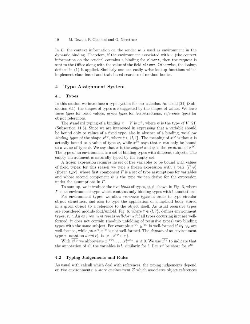
To sum up, we introduce the five kinds of types, ψ, φ, shown in Fig. 6, whereΓ is an environment type which contains only binding types with ! annotations.
For environment types, we allow recursive types in order to type circularobject structures, and also to type the application of a method body storedin a given object to a reference to the object itself. As usual recursive typesare considered modulo fold/unfold. Fig. 6, where † ∈ {!, ?}, defines environmenttypes, τ, ν. An environment type is well-formed if all types occurring in it are well-formed, it does not contain (modulo unfolding of recursive types) two bindingtypes with the same subject. For example x!ψ1 , y?ψ2 is well-formed if ψ1, ψ2 arewell-formed, while µt.x!t, x?ψ is not well-formed. The domain of an environmenttype τ , notation dom(τ), is {x | x†ψ ∈ τ}.
With x†ψ we abbreviate x†1ψ11 , . . . , x†nψn
n , n ≥ 0. We use x!ψ to indicate thatthe annotation of all the variables is !, similarly for ?. Let xψ be short for x!ψ.
4.2 Typing Judgements and Rules
As usual with calculi which deal with references, the typing judgements dependon two environments: a store environment Σ which associates object references
A Calculus of Evolving Objects 11
ψ, φ ::= κ Basic type| ψ → ψ Arrow type| refτ Reference type| 〈Γ, ψ〉 Frozen type| τ Environment type
τ, ν ::= x†ψ Binding type| τ, τ Sequence type| t Type variable| µt.τ Recursive type
Fig. 6. Kinds of Types and Environment Types
to types and a standard environment Γ which associates variables to types [21](Section 13.4). Then we define
Σ = ι : τΓ = x!ψ.
The typing judgment:Σ;Γ ` A : ψ
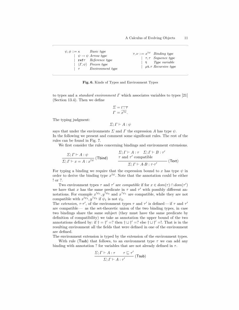
says that under the environments Σ and Γ the expression A has type ψ.In the following we present and comment some significant rules. The rest of therules can be found in Fig. 7.
We first consider the rules concerning bindings and environment extensions.
Σ;Γ ` A : ψ(Tbind)
Σ;Γ ` x = A : x†ψ
Σ;Γ ` A : τ Σ;Γ ` B : τ ′
τ and τ ′ compatible(Text)
Σ;Γ ` A·B : τ ·τ ′
For typing a binding we require that the expression bound to x has type ψ inorder to derive the binding type x†ψ. Note that the annotation could be either! or ?.
Two environment types τ and τ ′ are compatible if for x ∈ dom(τ) ∩ dom(τ ′)we have that x has the same predicate in τ and τ ′ with possibly different an-notations. For example x!ψ1 , y?ψ2 and x?ψ1 are compatible, while they are notcompatible with x!ψ2 , y?ψ2 if ψ1 is not ψ2.The extension, τ ·τ ′, of the environment types τ and τ ′ is defined— if τ and τ ′
are compatible — as the set-theoretic union of the two binding types, in casetwo bindings share the same subject (they must have the same predicate bydefinition of compatibility) we take as annotation the upper bound of the twoannotations defined by: if † = †′ =? then † t †′ =? else † t †′ =!. That is in theresulting environment all the fields that were defined in one of the environmentare defined.The environment extension is typed by the extension of the environment types.
With rule (Tsub) that follows, to an environment type τ we can add anybinding with annotation ? for variables that are not already defined in τ .
Σ;Γ ` A : τ τ v τ ′
(Tsub)Σ;Γ ` A : τ ′
12 M. Dezani, P. Giannini and O. Nierstrasz
(Tempty)Σ;Γ ` () : ∅
(TBV)Σ;Γ ` bv : κ
Σ;Γ ·xψ ` A : φ(Tabs)
Σ;Γ ` λx.A : ψ → φ
Σ;Γ ` A : φ→ ψ Σ;Γ ` B : φ(Tapp)
Σ;Γ ` A B : ψ
xψ ∈ Γ(Tvar)
Σ;Γ ` x : ψ
xψ ∈ Γ Σ;Γ ` E : $(TvarRT)
Σ;Γ ` (x)E : ψ
Σ;Γ ` A : τ(Tnew)
Σ;Γ ` new(A) : refτ
ι : τ ∈ Σ(Tref)
Σ;Γ ` ι : refτ
Σ;Γ ` A : refτ(Tderef)
Σ;Γ ` ∗A : τ
Σ;Γ ` A : refτ Σ;Γ ` B : ψ′ τ = µt.m†ψ, lkp!φ, ctx!$, τ ′
ψ = reft → ψ′ → ψ′′ φ = $ → reft → 〈mψ, ψ〉 → ψ t not in ψ′
(Tmes)Σ;Γ ` A m(B) : ψ′′[τ/t]
Fig. 7. Some Typing Rules
∅;Γ ` s : refτ
∅;Γ ` ∗s : τ ∅;Γ ` m : 〈mψ, ψ〉
D ∅;Γ ` m : 〈mψ, ψ〉
∅;Γ ` A w (∗s; d) m : ψ
∅;Γ ` (∗s)◦m�A w (∗s; d) m : ψ
∅; {w : $, s : refτ} ` λm.(∗s)◦m�A w (∗s; d) m : 〈mψ, ψ〉 → ψ
∅; {w : $} ` λs.λm.(∗s)◦m�A w (∗s; d) m : refτ → 〈mψ, ψ〉 → ψ
∅; ∅ ` λw.λs.λm.(∗s)◦m�A w (∗s; d) m : $ → refτ → 〈mψ, ψ〉 → ψ
where
D =
D′ ∅;Γ ` w : $
∅;Γ ` A w : refτ ′ → 〈mψ, ψ〉 → ψ
∅;Γ ` ∗s : τ ∅; drefτ′` d : refτ ′
∅;Γ ` ∗s; d : refτ ′
∅;Γ ` A w (∗s; d) : 〈mψ, ψ〉 → ψ
D′ =
∅;Γ ` ∗s; d : refτ ′
∅;Γ ` ∗(∗s; d) : τ
∅;Γ ` A : $ → refτ ′ → 〈mψ, ψ〉 → ψ
A = (∗(∗s; d)); lkp, d = delegate, Γ = {w : $, s : ψ,m : 〈mψ, ψ〉},τ ′ = µt.lkpφ, ν, φ = $ → reft → 〈mψ, ψ〉 → ψ.
Fig. 8. A Typing of the Lookup Function Ld
A Calculus of Evolving Objects 13
where the subtyping relation, v, between environment types is the reflexive andtransitive closure of:
φ v φ′ x 6∈ dom(φ′)(envAS)
φ v φ′, x?ψ
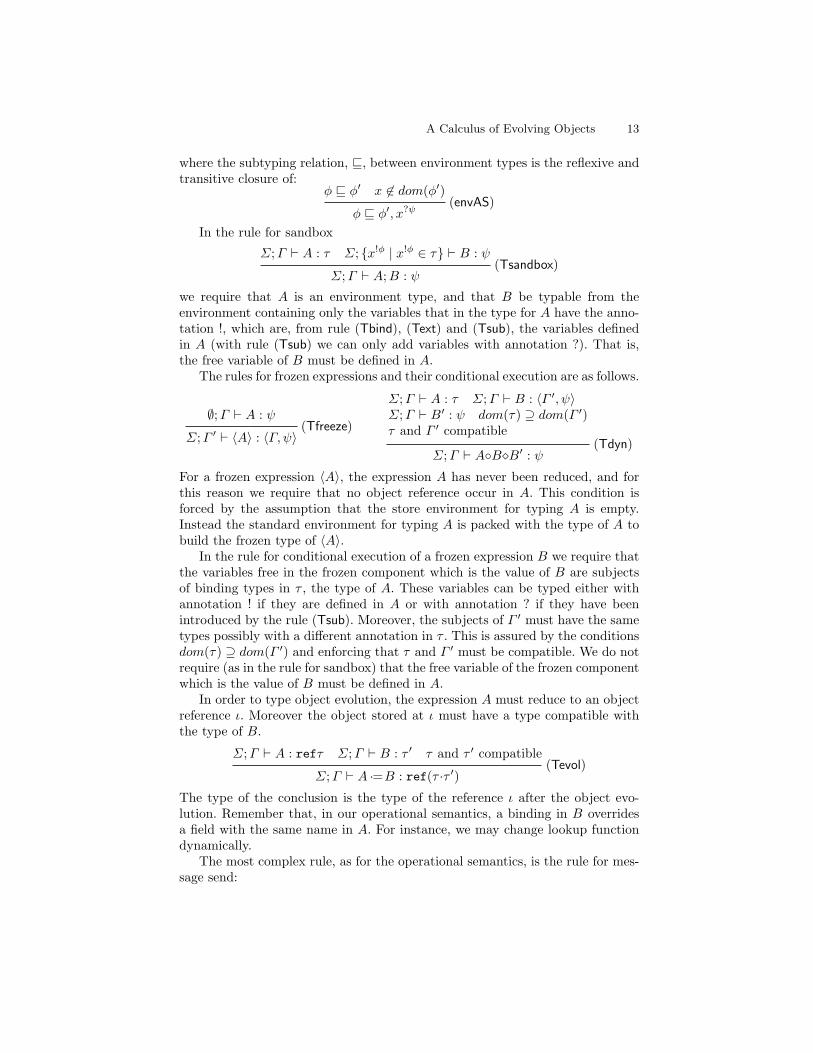
In the rule for sandbox
Σ;Γ ` A : τ Σ; {x!φ | x!φ ∈ τ} ` B : ψ(Tsandbox)
Σ;Γ ` A;B : ψ
we require that A is an environment type, and that B be typable from theenvironment containing only the variables that in the type for A have the anno-tation !, which are, from rule (Tbind), (Text) and (Tsub), the variables definedin A (with rule (Tsub) we can only add variables with annotation ?). That is,the free variable of B must be defined in A.
The rules for frozen expressions and their conditional execution are as follows.
∅;Γ ` A : ψ(Tfreeze)
Σ;Γ ′ ` 〈A〉 : 〈Γ, ψ〉
Σ;Γ ` A : τ Σ;Γ ` B : 〈Γ ′, ψ〉Σ;Γ ` B′ : ψ dom(τ) ⊇ dom(Γ ′)τ and Γ ′ compatible
(Tdyn)Σ;Γ ` A◦B�B′ : ψ
For a frozen expression 〈A〉, the expression A has never been reduced, and forthis reason we require that no object reference occur in A. This condition isforced by the assumption that the store environment for typing A is empty.Instead the standard environment for typing A is packed with the type of A tobuild the frozen type of 〈A〉.
In the rule for conditional execution of a frozen expression B we require thatthe variables free in the frozen component which is the value of B are subjectsof binding types in τ , the type of A. These variables can be typed either withannotation ! if they are defined in A or with annotation ? if they have beenintroduced by the rule (Tsub). Moreover, the subjects of Γ ′ must have the sametypes possibly with a different annotation in τ . This is assured by the conditionsdom(τ) ⊇ dom(Γ ′) and enforcing that τ and Γ ′ must be compatible. We do notrequire (as in the rule for sandbox) that the free variable of the frozen componentwhich is the value of B must be defined in A.
In order to type object evolution, the expression A must reduce to an objectreference ι. Moreover the object stored at ι must have a type compatible withthe type of B.
Σ;Γ ` A : refτ Σ;Γ ` B : τ ′ τ and τ ′ compatible(Tevol)
Σ;Γ ` A ·=B : ref(τ ·τ ′)
The type of the conclusion is the type of the reference ι after the object evo-lution. Remember that, in our operational semantics, a binding in B overridesa field with the same name in A. For instance, we may change lookup functiondynamically.
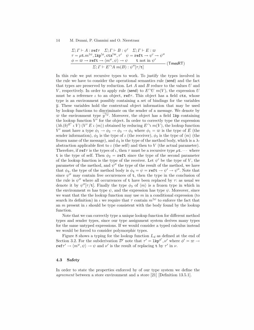
The most complex rule, as for the operational semantics, is the rule for mes-sage send:
14 M. Dezani, P. Giannini and O. Nierstrasz
Σ;Γ ` A : refτ Σ;Γ ` B : ψ′ Σ;Γ ` E : $τ = µt.m†ψ, lkp!φ, ctx!$, τ ′ ψ = reft→ ψ′ → ψ′′
φ = $ → reft→ 〈mψ, ψ〉 → ψ t not in ψ′(TmesRT)
Σ;Γ ` EyA m(B) : ψ′′[τ/t]
In this rule we put recursive types to work. To justify the types involved inthe rule we have to consider the operational semantics rule (send) and the factthat types are preserved by reduction. Let A and B reduce to the values U andV , respectively. In order to apply rule (send) to EyU m(V ), the expression Umust be a reference ι to an object, refτ . This object has a field ctx, whosetype is an environment possibly containing a set of bindings for the variablesy. These variables hold the contextual object information that may be usedby lookup functions to discriminate on the sender of a message. We denote by$ the environment type y?ψ. Moreover, the object has a field lkp containingthe lookup function V ′ for the object. In order to correctly type the expression(λb.(b)E
′ι V ) (V ′ E ι 〈m〉) obtained by reducing Eyι m(V ), the lookup function
V ′ must have a type φ1 → φ2 → φ3 → φ4 where φ1 = $ is the type of E (thesender information), φ2 is the type of ι (the receiver), φ3 is the type of 〈m〉 (thefrozen name of the message), and φ4 is the type of the method body, which is a λ-abstraction applicable first to ι (the self) and then to V (the actual parameter).Therefore, if refτ is the types of ι, then τ must be a recursive type µt. · · · wheret is the type of self. Then φ2 = reft since the type of the second parameterof the lookup function is the type of the receiver. Let ψ′ be the type of V , theparameter of the method, and ψ′′ the type of the result of the method, we havethat φ4, the type of the method body is φ4 = ψ = reft → ψ′ → ψ′′. Note thatsince ψ′′ may contain free occurrences of t, then the type in the conclusion ofthe rule is ψ′′ where all occurrences of t have been replaced by τ : as usual wedenote it by ψ′′[τ/t]. Finally the type φ3 of 〈m〉 is a frozen type in which inthe environment m has type ψ, and the expression has type ψ. Moreover, sincewe want that the the lookup function may use m in a conditional expression (tosearch its definition) in ι we require that τ contain m†ψ to enforce the fact thatan m present in ι should be type consistent with the body found by the lookupfunction.
Note that we can correctly type a unique lookup function for different methodtypes and sender types, since our type assignment system derives many typesfor the same untyped expressions. If we would consider a typed calculus insteadwe would be forced to consider polymorphic types.
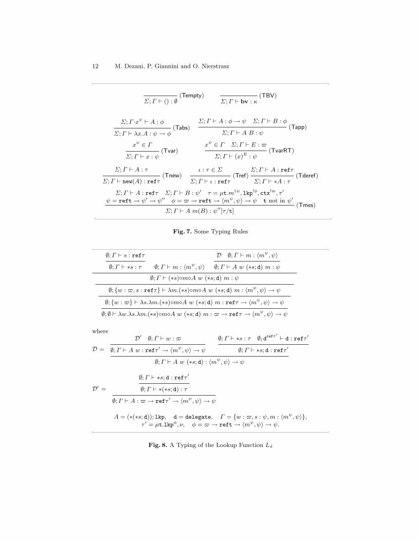
Figure 8 shows a typing for the lookup function Ld as defined at the end ofSection 3.2. For the subderivation D′ note that τ ′ = lkpφ
′, ν′ where φ′ = $ →
refτ ′ → 〈mψ, ψ〉 → ψ and ν′ is the result of replacing t by τ ′ in ν.
4.3 Safety
In order to state the properties enforced by of our type system we define theagreement between a store environment and a store [21] [Definition 13.5.1].
A Calculus of Evolving Objects 15
Definition 1. A store environment Σ agrees with a memory σ (notation Σ ` σ)if:
– σ(ι) = E implies ι : τ ∈ Σ and Σ; ∅ ` E : τ for some τ , and– ι : τ ∈ Σ implies σ(ι) = E and Σ; ∅ ` E : τ for some E.
Reducing expressions modifies the store, and for this reason also the store envi-ronment needs to evolve.
Definition 2. We say that a store environment Σ′ is an evolution of a storeenvironment Σ if ι : τ ∈ Σ implies ι : τ ·τ ′ ∈ Σ′ for some τ ′ compatible with τ .
The two results insuring that well-typed expressions do not get stuck are:
Theorem 1 (Subject Reduction). If Σ;Γ ` A : ψ and Σ ` σ and A, σ →B, σ′, then Σ′;Γ ` B : ψ and Σ′ ` σ′ for some evolution Σ′ of Σ.
Theorem 2 (Progress). If Σ; ∅ ` A : ψ and Σ ` σ and A is not a value, thenthere are unique B′, σ′ such that A, σ → B, σ′.
Subject Reduction also assures that:
– variables in an evolving environment are bound to values of fixed types;– the free variables in the body of a sandbox are always bound in the environ-
ment of the sandbox.
5 Related work
Abadi et al. were the first to study explicit substitutions as a way to bridge thegap between formal models of languages and concrete implementations [2]. Thesymmetric Lisp supports environments as first class objects, since it does notdistinguish between data and programs [14]. Nishizaki developed a calculus offirst-class environments in order to study dynamic software evolution [20]. Thiscalculus is purely functional and does not model objects or message sends.
The Piccola calculus [3] extended Milner’s π-calculus [16] with first-classenvironments as a means to study and model software composition mechanisms.The functional core of the Piccola calculus, called the form calculus [18], hasbeen used to study type inference for component-based service provision. Avariant of the form calculus has also been studied by Lumpe and Schneider as ameta-framework for modeling composition mechanisms [15]. The object calculusdescribed in the present paper can be seen as the form calculus, extended withan explicit object store, object references, message sending.
Harrison and Ossher introduced the notion of subject-oriented programmingto acknowledge the fact that behaviour does not always depend only on the re-ceiver of a message but also its sender [11]. Smith and Ungar demonstrated howsubjectivity could be realized effectively, and how it solves numerous problems re-lated to the context-dependent behaviour [24]. Gil and Lorenz proposed environ-mental acquisition in which objects acquire behaviour from the current contain-ers at runtime [10]. More recently, context-oriented programming has emerged
16 M. Dezani, P. Giannini and O. Nierstrasz
as a way to support multi-dimensional dispatch in object-oriented languages,and thus to adapt behaviour to the run-time context [13]. In the same strand[17] considers contextual effects, i.e. the effects of the computational contexts inwhich expressions occur.
It is well-know that code migration requires dynamic reconfiguration of secu-rity policies: an interesting proposal is [12]. More difficult is modelling exchangeof open mobile code, i.e. code which may contain free variables to be boundby the receiver’s code [8]. Ancona, Fagorzi and Zucca provide a combination ofstatic and dynamic checks which assures type safety for mobile open code [4].
Type annotations are used by Damiani and Giannini [9] to discriminatewhether a given field is defined or undefined in an object. Anderson and Gian-nini [5] used “defined/maybe” annotations on types and recursive types in anobject based calculus in which fields may be added to objects. Recursive typesare used, in a limited way, to type an object’s “self” as well as functions return-ing functions. An inference algorithm has also been defined for this type system[6]. In both calculi message send is identified with method call [9] [5].
6 Concluding remarks
We have presented a novel object calculus in which message sends are dynami-cally looked up, taking into account contextual information such as the identityof the sender. Objects can evolve over time, as can the lookup function itself.Method bodies may contain free variables which are dynamically bound whenthe method is invoked. First-class environments and “freezing” of expressionswith free variables are the key mechanisms used to express dynamic binding.
Despite the highly dynamic nature of the calculus, we have demonstratedhow a type assignment system can provide the usual safety guarantees.
We plan to design a type inference algorithm for the present system: this willbe useful for experimenting with the present calculus without having the burdenof checking typeability.
References
1. Martın Abadi and Luca Cardelli. A Theory of Objects. Springer-Verlag, 1996.
2. Martın Abadi, Luca Cardelli, Pierre-Louis Curien, and Jean-Jacques Levy. Explicitsubstitutions. Journal of Functional Programming, 1(4):375–416, 1991.
3. Franz Achermann and Oscar Nierstrasz. A calculus for reasoning about softwarecomponents. Theoretical Computer Science, 331(2-3):367–396, 2005.
4. Davide Ancona, Sonia Fagorzi, and Elena Zucca. A parametric calculus for mobileopen code. In DCM’07, ENTCS. Elsevier, 2008. To appear.
5. Christopher Anderson and Paola Giannini. Type checking for JavaScript. InWOOD’05, volume 138 of ENTCS, pages 37–58. Elsevier, 2005.
6. Christopher Anderson, Paola Giannini, and Sophia Drossopoulou. Towards typeinference for Javascript. In ECOOP’05, volume 3586 of LNCS, pages 428–453.Springer, 2005.

A Calculus of Evolving Objects 17
7. Alexandre Bergel and Stephane Ducasse. Supporting unanticipated changes withTraits and Classboxes. In NODe’05, volume 69 of LNI, pages 61–75. GI, 2005.
8. Gavin Bierman, Michael Hicks, Peter Sewell, Gareth Stoyle, and Keith Wans-brough. Dynamic rebinding for marshalling and update, with destruct-time λ. InICFP’03, pages 99–110. ACM, 2003.
9. Ferruccio Damiani and Paola Giannini. Alias types for “environment-aware” com-putations. In WOOD’03, volume 82 of ENTCS, pages 130–150. Elsevier, 2003.
10. Joseph Gil and David H. Lorenz. Environmental acquisition - a new inheritance-likeabstraction mechanism. In OOPSLA’96, volume 31 of ACM SIGPLAN Notices,pages 214–231, 1996.
11. William Harrison and Harold Ossher. Subject-oriented programming (a critiqueof pure objects). In OOPSLA’93, volume 28 of ACM SIGPLAN Notices, pages411–428, 1993.
12. Brant Hashii, Scott Malabarba, Raju Pandey, and Matt Bishop. Supporting re-configurable security policies for mobile programs. Computer Networks, 33:77–93,200.
13. Robert Hirschfeld, Pascal Costanza, and Oscar Nierstrasz. Context-oriented pro-gramming. Journal of Object Technology, 7(3), March 2008.
14. Suresh Jagannathan. A Programming Language Supporting First-Class ParallelEnvironments. PhD thesis, M.I.T., 1989.
15. Markus Lumpe and Jean-Guy Schneider. A form-based metamodel for softwarecomposition. Journal of Science of Computer Programming, 56(2):59–78, 2005.
16. Robin Milner, Joachim Parrow, and David Walker. A calculus of mobile processes,part I/II. Information and Computation, 100:1–77, 1992.
17. Iulian Neamtiu, Michael Hicks, Jeffrey S. Foster, and Polyvios Pratikakis. Contex-tual effects for version-consistent dynamic software updating and safe concurrentprogramming. In POPL’08, pages 37–50. ACM, 2008.
18. Oscar Nierstrasz. Contractual types. Technical Report IAM-03-004, Institute ofComputer Science, University of Bern, Switzerland, 2003.
19. Oscar Nierstrasz, Alexandre Bergel, Marcus Denker, Stephane Ducasse, MarkusGaelli, and Roel Wuyts. On the revival of dynamic languages. In Software Com-position’05, volume 3628 of LNCS, pages 1–13. Springer, 2005. Invited paper.
20. Shin-ya Nishizaki. Programmable environment calculus as theory of dynamic soft-ware evolution. In ISPSE’00, pages 221–225. IEEE Computer Society Press, 2000.
21. Benjamin C. Pierce. Types and Programming Languages. MIT Press, 2002.
22. David Rothlisberger, Marcus Denker, and Eric Tanter. Unanticipated partial be-havioral reflection: Adapting applications at runtime. Journal of Computer Lan-guages, Systems and Structures, 34(2-3):46–65, July 2008.
23. Peter Seibel. Practical CommonLisp. Apress, 2005.
24. Randall B. Smith and Dave Ungar. A simple and unifying approach to subjectiveobjects. TAPOS special issue on Subjectivity in Object-Oriented Systems, 2(3):161–178, 1996.
18 M. Dezani, P. Giannini and O. Nierstrasz
A Appendix
A.1 Proof of Soundness
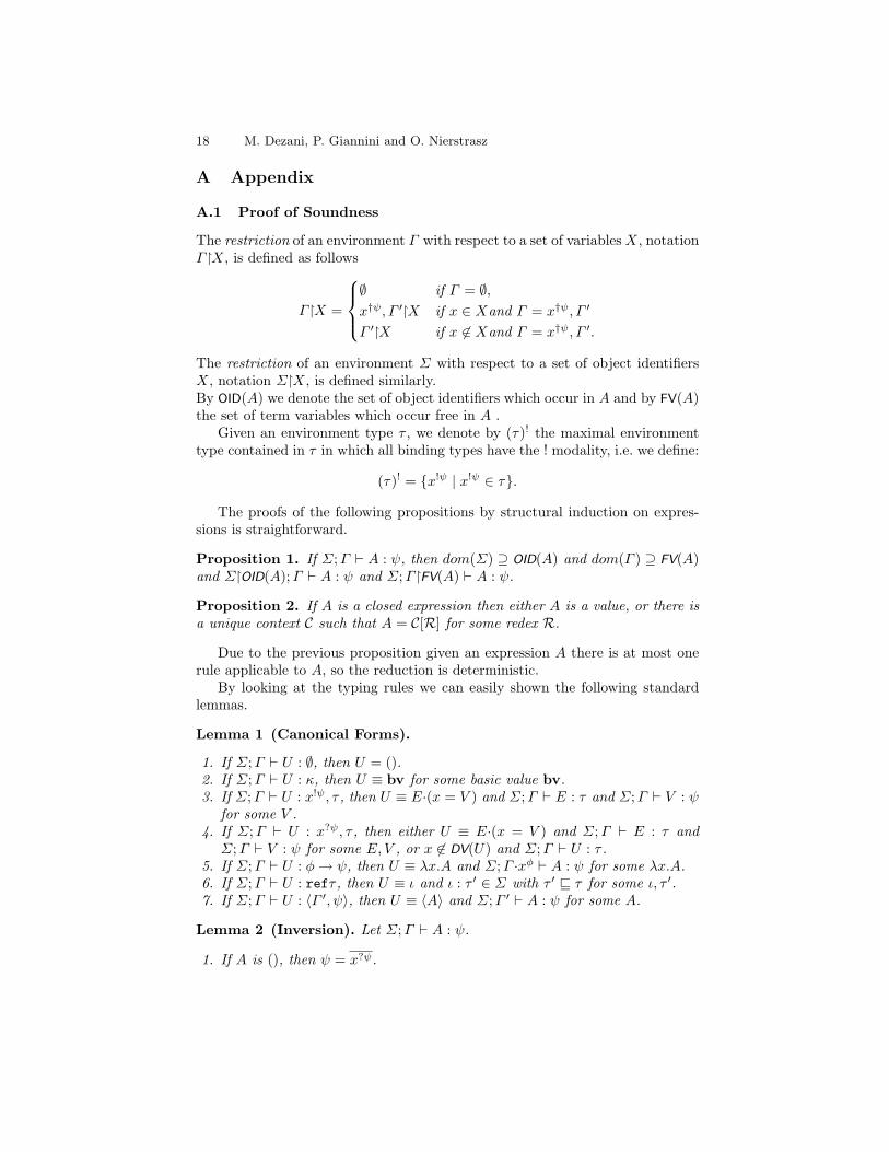
The restriction of an environment à with respect to a set of variablesX, notation�X, is defined as follows
Γ�X =
∅ if Γ = ∅,x†ψ, Γ ′�X if x ∈ Xand Γ = x†ψ, Γ ′
Γ ′�X if x 6∈ Xand Γ = x†ψ, Γ ′.
The restriction of an environment Σ with respect to a set of object identifiersX, notation Σ�X, is defined similarly.By OID(A) we denote the set of object identifiers which occur in A and by FV(A)the set of term variables which occur free in A .
Given an environment type τ , we denote by (τ)! the maximal environmenttype contained in τ in which all binding types have the ! modality, i.e. we define:
(τ)! = {x!ψ | x!ψ ∈ τ}.
The proofs of the following propositions by structural induction on expres-sions is straightforward.
Proposition 1. If Σ;Γ ` A : ψ, then dom(Σ) ⊇ OID(A) and dom(Γ ) ⊇ FV(A)and Σ�OID(A);Γ ` A : ψ and Σ;Γ�FV(A) ` A : ψ.
Proposition 2. If A is a closed expression then either A is a value, or there isa unique context C such that A = C[R] for some redex R.
Due to the previous proposition given an expression A there is at most onerule applicable to A, so the reduction is deterministic.
By looking at the typing rules we can easily shown the following standardlemmas.
Lemma 1 (Canonical Forms).
1. If Σ;Γ ` U : ∅, then U = ().2. If Σ;Γ ` U : κ, then U ≡ bv for some basic value bv.3. If Σ;Γ ` U : x!ψ, τ , then U ≡ E·(x = V ) and Σ;Γ ` E : τ and Σ;Γ ` V : ψ
for some V .4. If Σ;Γ ` U : x?ψ, τ , then either U ≡ E·(x = V ) and Σ;Γ ` E : τ and
Σ;Γ ` V : ψ for some E, V , or x 6∈ DV(U) and Σ;Γ ` U : τ .5. If Σ;Γ ` U : φ→ ψ, then U ≡ λx.A and Σ;Γ ·xφ ` A : ψ for some λx.A.6. If Σ;Γ ` U : refτ , then U ≡ ι and ι : τ ′ ∈ Σ with τ ′ v τ for some ι, τ ′.7. If Σ;Γ ` U : 〈Γ ′, ψ〉, then U ≡ 〈A〉 and Σ;Γ ′ ` A : ψ for some A.
Lemma 2 (Inversion). Let Σ;Γ ` A : ψ.
1. If A is (), then ψ = x?ψ.
A Calculus of Evolving Objects 19
2. If A is a basic value, then ψ = κ, for some basic type κ.3. If A is x, then for some ψ′ we have that xψ
′ ∈ Γ and ψ′ v ψ.4. If A is 〈B〉, then ψ = 〈Γ ′, ψ′〉 and Σ;Γ ′ ` B : ψ′ for some Γ ′, ψ′.5. If A is x=B, then ψ = x†ψ′
, x?ψ, and Σ;Γ ` B : ψ′ for some ψ′, x?ψ.6. If A is λx.B, then ψ = ψ′ → φ and Σ;Γ ·xψ′ ` B : φ for some ψ′, φ.7. If A is B·C, then ψ = τ ·τ ′ and Σ;Γ ` B : τ and Σ;Γ ` C : τ ′ for some
compatible τ, τ ′.8. If A is B;C, then Σ;Γ ` B : τ and Σ; (τ)! ` C : ψ for some τ .9. If A is B◦C�C ′, then Σ;Γ ` B : τ , and Σ;Γ ` C : 〈Γ ′, ψ〉, and Σ;Γ ` C ′ :
ψ, and dom(τ) ⊇ dom(Γ ′), for some compatible τ, Γ ′ .10. If A is B C, then Σ;Γ ` B : ψ′ → φ and Σ;Γ ` C : ψ′ and φ v ψ for some
φ, ψ′.11. If A is ι, then ψ = refτ and ι : τ ′ ∈ Σ for some τ ′ v τ .12. If A is ∗B, then Σ;Γ ` B : refψ.13. If A is new(B), then ψ = refτ and Σ;Γ ` B : τ for some τ .14. If A is B ·=C, then ψ = ref(τ ·τ ′) and Σ;Γ ` B : refτ and Σ;Γ ` C : τ ′
for some compatible τ, τ ′.15. If A is B m(C), then ψ = ψ′′[τ/t] and Σ;Γ ` B : refτ and Σ;Γ ` C : ψ′
and τ = µt.m†φ′, lkp!φ, ctx!$, τ ′ and φ′ = reft → ψ′ → ψ′′ and φ = $ →
reft → 〈mφ′, φ′〉 → φ′ for some φ, φ′, ψ′, ψ′′, $ = y?ψ such that t does not
occur in φ′.16. If A is EyB m(C), then ψ = ψ′′[τ/t] and Σ;Γ ` B : refτ and Σ;Γ ` C : ψ′
and Σ;Γ ` E : $ and τ = µt.m†φ′, lkp!φ, ctx!$, τ ′ and φ′ = reft → ψ′ →
ψ′′ and φ = $ → reft → 〈mφ′, φ′〉 → φ′ for some φ, φ′, ψ′, ψ′′, $ = y?ψ
such that t does not occur in φ′.
Lemma 3 (Weakening). If Σ;Γ ` A : ψ, and Γ ′ ⊇ Γ , then Σ;Γ ′ ` A : ψ.
Lemma 4. 1. If Σ;Γ ` A : ψ, and A = C[R], then Σ;Γ ` R : ψ′ for some ψ′.2. If Σ;Γ ` C[R] : ψ where Σ;Γ ` R : ψ′, and Σ;Γ ` A : ψ′, then Σ;Γ `
C[A] : ψ.
Proof. By induction on evaluation contexts.
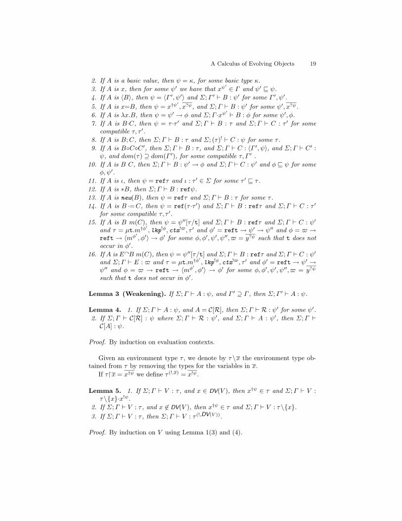
Given an environment type τ , we denote by τ \x the environment type ob-tained from τ by removing the types for the variables in x.
If τ�x = x†ψ we define τ (!,x) = x!ψ.
Lemma 5. 1. If Σ;Γ ` V : τ , and x ∈ DV(V ), then x†ψ ∈ τ and Σ;Γ ` V :τ \{x}·x!ψ.
2. If Σ;Γ ` V : τ , and x 6∈ DV(V ), then x†ψ ∈ τ and Σ;Γ ` V : τ \{x}.3. If Σ;Γ ` V : τ , then Σ;Γ ` V : τ (!,DV(V )).
Proof. By induction on V using Lemma 1(3) and (4).
20 M. Dezani, P. Giannini and O. Nierstrasz
Proof of Subject Reduction
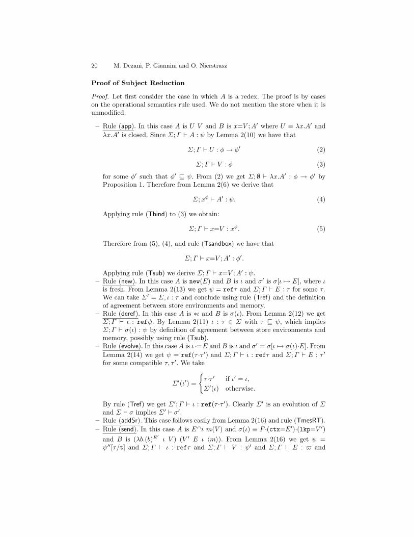
Proof. Let first consider the case in which A is a redex. The proof is by caseson the operational semantics rule used. We do not mention the store when it isunmodified.
– Rule (app). In this case A is U V and B is x=V ;A′ where U ≡ λx.A′ andλx.A′ is closed. Since Σ;Γ ` A : ψ by Lemma 2(10) we have that
Σ;Γ ` U : φ→ φ′ (2)
Σ;Γ ` V : φ (3)
for some φ′ such that φ′ v ψ. From (2) we get Σ; ∅ ` λx.A′ : φ → φ′ byProposition 1. Therefore from Lemma 2(6) we derive that
Σ;xφ ` A′ : ψ. (4)
Applying rule (Tbind) to (3) we obtain:
Σ;Γ ` x=V : xφ. (5)
Therefore from (5), (4), and rule (Tsandbox) we have that
Σ;Γ ` x=V ;A′ : φ′.
Applying rule (Tsub) we derive Σ;Γ ` x=V ;A′ : ψ.– Rule (new). In this case A is new(E) and B is ι and σ′ is σ[ι 7→ E], where ι
is fresh. From Lemma 2(13) we get ψ = refτ and Σ;Γ ` E : τ for some τ .We can take Σ′ = Σ, ι : τ and conclude using rule (Tref) and the definitionof agreement between store environments and memory.
– Rule (deref). In this case A is ∗ι and B is σ(ι). From Lemma 2(12) we getΣ;Γ ` ι : refψ. By Lemma 2(11) ι : τ ∈ Σ with τ v ψ, which impliesΣ;Γ ` σ(ι) : ψ by definition of agreement between store environments andmemory, possibly using rule (Tsub).
– Rule (evolve). In this case A is ι ·=E and B is ι and σ′ = σ[ι 7→ σ(ι)·E]. FromLemma 2(14) we get ψ = ref(τ ·τ ′) and Σ;Γ ` ι : refτ and Σ;Γ ` E : τ ′
for some compatible τ, τ ′. We take
Σ′(ι′) =
{τ ·τ ′ if ι′ = ι,
Σ′(ι) otherwise.
By rule (Tref) we get Σ′;Γ ` ι : ref(τ ·τ ′). Clearly Σ′ is an evolution of Σand Σ ` σ implies Σ′ ` σ′.
– Rule (addSr). This case follows easily from Lemma 2(16) and rule (TmesRT).– Rule (send). In this case A is Eyι m(V ) and σ(ι) ≡ F ·(ctx=E′)·(lkp=V ′)
and B is (λb.(b)E′ι V ) (V ′ E ι 〈m〉). From Lemma 2(16) we get ψ =
ψ′′[τ/t] and Σ;Γ ` ι : refτ and Σ;Γ ` V : ψ′ and Σ;Γ ` E : $ and
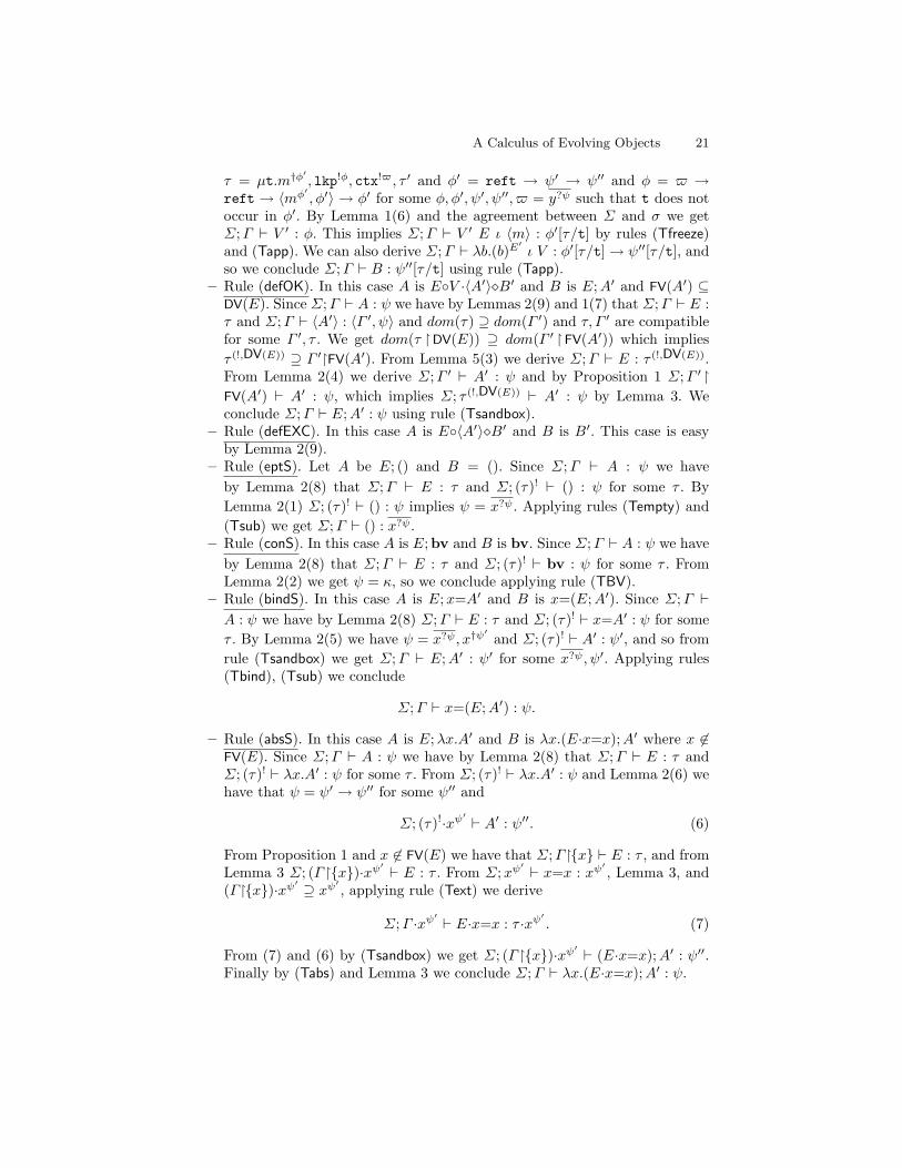
A Calculus of Evolving Objects 21
τ = µt.m†φ′, lkp!φ, ctx!$, τ ′ and φ′ = reft → ψ′ → ψ′′ and φ = $ →
reft → 〈mφ′, φ′〉 → φ′ for some φ, φ′, ψ′, ψ′′, $ = y?ψ such that t does not
occur in φ′. By Lemma 1(6) and the agreement between Σ and σ we getΣ;Γ ` V ′ : φ. This implies Σ;Γ ` V ′ E ι 〈m〉 : φ′[τ/t] by rules (Tfreeze)and (Tapp). We can also derive Σ;Γ ` λb.(b)E′
ι V : φ′[τ/t] → ψ′′[τ/t], andso we conclude Σ;Γ ` B : ψ′′[τ/t] using rule (Tapp).
– Rule (defOK). In this case A is E◦V ·〈A′〉�B′ and B is E;A′ and FV(A′) ⊆DV(E). Since Σ;Γ ` A : ψ we have by Lemmas 2(9) and 1(7) that Σ;Γ ` E :τ and Σ;Γ ` 〈A′〉 : 〈Γ ′, ψ〉 and dom(τ) ⊇ dom(Γ ′) and τ, Γ ′ are compatiblefor some Γ ′, τ . We get dom(τ �DV(E)) ⊇ dom(Γ ′ �FV(A′)) which impliesτ (!,DV(E)) ⊇ Γ ′�FV(A′). From Lemma 5(3) we derive Σ;Γ ` E : τ (!,DV(E)).From Lemma 2(4) we derive Σ;Γ ′ ` A′ : ψ and by Proposition 1 Σ;Γ ′ �FV(A′) ` A′ : ψ, which implies Σ; τ (!,DV(E)) ` A′ : ψ by Lemma 3. Weconclude Σ;Γ ` E;A′ : ψ using rule (Tsandbox).
– Rule (defEXC). In this case A is E◦〈A′〉�B′ and B is B′. This case is easyby Lemma 2(9).
– Rule (eptS). Let A be E; () and B = (). Since Σ;Γ ` A : ψ we haveby Lemma 2(8) that Σ;Γ ` E : τ and Σ; (τ)! ` () : ψ for some τ . ByLemma 2(1) Σ; (τ)! ` () : ψ implies ψ = x?ψ. Applying rules (Tempty) and(Tsub) we get Σ;Γ ` () : x?ψ.
– Rule (conS). In this case A is E;bv and B is bv. Since Σ;Γ ` A : ψ we haveby Lemma 2(8) that Σ;Γ ` E : τ and Σ; (τ)! ` bv : ψ for some τ . FromLemma 2(2) we get ψ = κ, so we conclude applying rule (TBV).
– Rule (bindS). In this case A is E;x=A′ and B is x=(E;A′). Since Σ;Γ `A : ψ we have by Lemma 2(8) Σ;Γ ` E : τ and Σ; (τ)! ` x=A′ : ψ for someτ . By Lemma 2(5) we have ψ = x?ψ, x†ψ′
and Σ; (τ)! ` A′ : ψ′, and so fromrule (Tsandbox) we get Σ;Γ ` E;A′ : ψ′ for some x?ψ, ψ′. Applying rules(Tbind), (Tsub) we conclude
Σ;Γ ` x=(E;A′) : ψ.
– Rule (absS). In this case A is E;λx.A′ and B is λx.(E·x=x);A′ where x 6∈FV(E). Since Σ;Γ ` A : ψ we have by Lemma 2(8) that Σ;Γ ` E : τ andΣ; (τ)! ` λx.A′ : ψ for some τ . From Σ; (τ)! ` λx.A′ : ψ and Lemma 2(6) wehave that ψ = ψ′ → ψ′′ for some ψ′′ and
Σ; (τ)!·xψ′` A′ : ψ′′. (6)
From Proposition 1 and x 6∈ FV(E) we have that Σ;Γ�{x} ` E : τ , and fromLemma 3 Σ; (Γ �{x})·xψ′ ` E : τ . From Σ;xψ
′ ` x=x : xψ′, Lemma 3, and
(Γ�{x})·xψ′ ⊇ xψ′, applying rule (Text) we derive
Σ;Γ ·xψ′` E·x=x : τ ·xψ
′. (7)
From (7) and (6) by (Tsandbox) we get Σ; (Γ�{x})·xψ′ ` (E·x=x);A′ : ψ′′.Finally by (Tabs) and Lemma 3 we conclude Σ;Γ ` λx.(E·x=x);A′ : ψ.
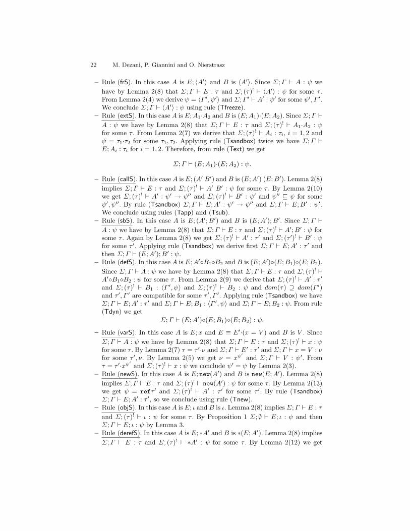
22 M. Dezani, P. Giannini and O. Nierstrasz
– Rule (frS). In this case A is E; 〈A′〉 and B is 〈A′〉. Since Σ;Γ ` A : ψ wehave by Lemma 2(8) that Σ;Γ ` E : τ and Σ; (τ)! ` 〈A′〉 : ψ for some τ .From Lemma 2(4) we derive ψ = 〈Γ ′, ψ′〉 and Σ;Γ ′ ` A′ : ψ′ for some ψ′, Γ ′.We conclude Σ;Γ ` 〈A′〉 : ψ using rule (Tfreeze).
– Rule (extS). In this case A is E;A1·A2 and B is (E;A1)·(E;A2). Since Σ;Γ `A : ψ we have by Lemma 2(8) that Σ;Γ ` E : τ and Σ; (τ)! ` A1·A2 : ψfor some τ . From Lemma 2(7) we derive that Σ; (τ)! ` Ai : τi, i = 1, 2 andψ = τ1·τ2 for some τ1, τ2. Applying rule (Tsandbox) twice we have Σ;Γ `E;Ai : τi for i = 1, 2. Therefore, from rule (Text) we get
Σ;Γ ` (E;A1)·(E;A2) : ψ.
– Rule (callS). In this case A is E; (A′ B′) and B is (E;A′) (E;B′). Lemma 2(8)implies Σ;Γ ` E : τ and Σ; (τ)! ` A′ B′ : ψ for some τ . By Lemma 2(10)we get Σ; (τ)! ` A′ : ψ′ → ψ′′ and Σ; (τ)! ` B′ : ψ′ and ψ′′ v ψ for someψ′, ψ′′. By rule (Tsandbox) Σ;Γ ` E;A′ : ψ′ → ψ′′ and Σ;Γ ` E;B′ : ψ′.We conclude using rules (Tapp) and (Tsub).
– Rule (sbS). In this case A is E; (A′;B′) and B is (E;A′);B′. Since Σ;Γ `A : ψ we have by Lemma 2(8) that Σ;Γ ` E : τ and Σ; (τ)! ` A′;B′ : ψ forsome τ . Again by Lemma 2(8) we get Σ; (τ)! ` A′ : τ ′ and Σ; (τ ′)! ` B′ : ψfor some τ ′. Applying rule (Tsandbox) we derive first Σ;Γ ` E;A′ : τ ′ andthen Σ;Γ ` (E;A′);B′ : ψ.
– Rule (defS). In this case A is E;A′◦B1�B2 and B is (E;A′)◦(E;B1)�(E;B2).Since Σ;Γ ` A : ψ we have by Lemma 2(8) that Σ;Γ ` E : τ and Σ; (τ)! `A′◦B1�B2 : ψ for some τ . From Lemma 2(9) we derive that Σ; (τ)! ` A′ : τ ′
and Σ; (τ)! ` B1 : 〈Γ ′, ψ〉 and Σ; (τ)! ` B2 : ψ and dom(τ) ⊇ dom(Γ ′)and τ ′, Γ ′ are compatible for some τ ′, Γ ′. Applying rule (Tsandbox) we haveΣ;Γ ` E;A′ : τ ′ and Σ;Γ ` E;B1 : 〈Γ ′, ψ〉 and Σ;Γ ` E;B2 : ψ. From rule(Tdyn) we get
Σ;Γ ` (E;A′)◦(E;B1)�(E;B2) : ψ.
– Rule (varS). In this case A is E;x and E ≡ E′·(x = V ) and B is V . SinceΣ;Γ ` A : ψ we have by Lemma 2(8) that Σ;Γ ` E : τ and Σ; (τ)! ` x : ψfor some τ . By Lemma 2(7) τ = τ ′·ν and Σ;Γ ` E′ : τ ′ and Σ;Γ ` x = V : νfor some τ ′, ν. By Lemma 2(5) we get ν = xψ
′and Σ;Γ ` V : ψ′. From
τ = τ ′·xψ′and Σ; (τ)! ` x : ψ we conclude ψ′ = ψ by Lemma 2(3).
– Rule (newS). In this case A is E; new(A′) and B is new(E;A′). Lemma 2(8)implies Σ;Γ ` E : τ and Σ; (τ)! ` new(A′) : ψ for some τ . By Lemma 2(13)we get ψ = refτ ′ and Σ; (τ)! ` A′ : τ ′ for some τ ′. By rule (Tsandbox)Σ;Γ ` E;A′ : τ ′, so we conclude using rule (Tnew).
– Rule (objS). In this case A is E; ι and B is ι. Lemma 2(8) impliesΣ;Γ ` E : τand Σ; (τ)! ` ι : ψ for some τ . By Proposition 1 Σ; ∅ ` E; ι : ψ and thenΣ;Γ ` E; ι : ψ by Lemma 3.
– Rule (derefS). In this case A is E; ∗A′ and B is ∗(E;A′). Lemma 2(8) impliesΣ;Γ ` E : τ and Σ; (τ)! ` ∗A′ : ψ for some τ . By Lemma 2(12) we get
A Calculus of Evolving Objects 23
Σ; (τ)! ` A′ : refψ. By rule (Tsandbox) Σ;Γ ` E;A′ : refψ, so we concludeusing rule (Tderef).
– Rule (evolS). In this case A is E; (A′ ·= B′) and B is (E;A′) ·= (E;B′).Lemma 2(8) implies Σ;Γ ` E : τ and Σ; (τ)! ` A′.=B′ : ψ for some τ . ByLemma 2(14) we get ψ = ref(τ ′·τ ′′) and Σ; (τ)! ` A′ : refτ ′ and Σ; (τ)! `B′ : τ ′′ for some compatible τ ′, τ ′′. By rule (Tsandbox) we get Σ;Γ ` E;A′ :refτ ′ and Σ;Γ ` E;B′ : τ ′′, so we conclude using rule (Tevol).
– Rule (sendS). This case is similar and simpler than the following case.– Rule (sendRTS). In this caseA is E; (FyA′ m(B′)) andB is (E;F )y(E;A′)m(E;B′).
Lemma 2(8) implies Σ;Γ ` E : τ and Σ; (τ)! ` FyA′ m(B′) : ψ for someτ . By Lemma 2(16) we get ψ = ψ′′[ν/t] and Σ; (τ)! ` A′ : refν andΣ; (τ)! ` B′ : ψ′ and Σ; (τ)! ` F : $ and ν = µt.m†φ′
, lkp!φ, ctx!$, ν′
and φ′ = reft → ψ′ → ψ′′ and φ = $ → reft → 〈mφ′, φ′〉 → φ′ for some
φ, φ′, ψ′, ψ′′, $ = y?ψ such that t does not occur in φ′. By rule (Tsandbox)we get Σ;Γ ` E;A′ : refν and Σ;Γ ` E;B′ : ψ′ and Σ;Γ ` E;F : $, sowe conclude using rule (TmesRT).
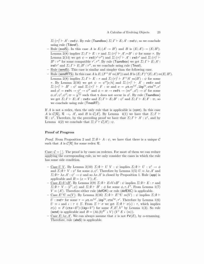
If A is not a redex, then the only rule that is applicable is (cont). In this caseA is C[R], R →r A
′, and B is C[A′]. By Lemma 4(1) we have that Σ;Γ `R : ψ′. Therefore, by the preceding proof we have that Σ;Γ ` A′ : ψ′, and byLemma 4(2) we conclude that Σ;Γ ` C[A′] : ψ.
Proof of Progress
Proof. From Proposition 2 and Σ; ∅ ` A : ψ, we have that there is a unique Csuch that A is C[R] for some redex R.
Case: C = [ ]. The proof is by cases on redexes. For most of them we can reduceapplying the corresponding rule, so we only consider the cases in which the rulehas some side condition.
– Case U V . By Lemma 2(10) Σ; ∅ ` U V : ψ implies Σ; ∅ ` U : ψ′ → φand Σ; ∅ ` V : ψ′ for some φ, ψ′. Therefore by Lemma 1(5) U ≡ λx.A′ andΣ; ∅ ` λx.A′ : ψ′ → ψ and so λx.A′ is closed by Proposition 1. Rule (app) isapplicable and B = (x = V );A′.
– Case E◦V �B′. By Lemma 2(9) Σ; ∅ ` E◦V �B′ : ψ implies Σ; ∅ ` E : τ andΣ; ∅ ` V : 〈Γ ′, ψ〉 and Σ; ∅ ` B′ : φ for some φ, τ, Γ ′. From Lemma 1(7)V ≡ 〈A′〉. Therefore either rule (defOK) or rule (defEXC) is applicable.
– Case EyU m(V ). By Lemma 2(16) Σ; ∅ ` EyU m(V ) : ψ implies Σ; ∅ `U : refτ for some τ = µt.m†φ′
, lkp!φ, ctx!$, τ ′. Therefore by Lemma 1(6)U ≡ ι and ι : τ ∈ Σ. From Σ ` σ we get Σ; ∅ ` σ(ι) : τ , which impliesσ(ι) ≡ F ·(ctx=E′)·(lkp=V ′) for some F,E′, V ′ by Lemma 1(3). So rule(send) is applicable and B = (λb.(b)E
′ι V ) (V ′ E ι 〈m〉).
– Case E;λx.A′. We can always assume that x is not FV(E), by α-renaming.Therefore, rule (absS) is applicable.
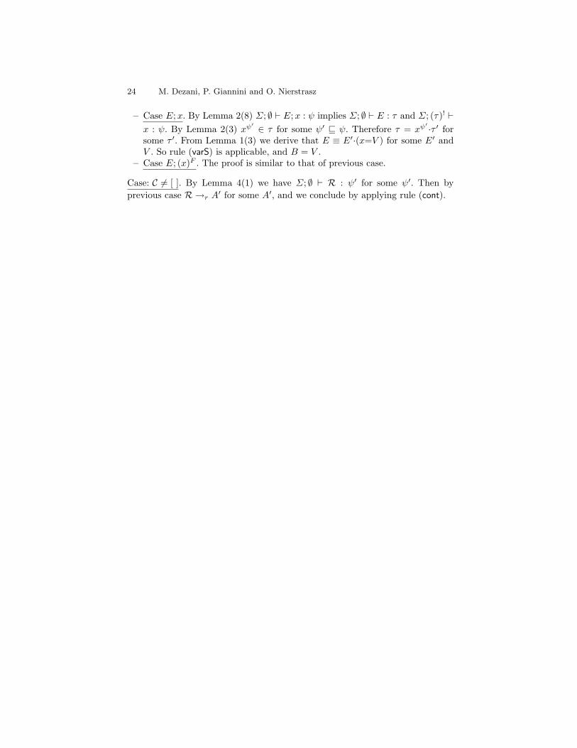
24 M. Dezani, P. Giannini and O. Nierstrasz
– Case E;x. By Lemma 2(8) Σ; ∅ ` E;x : ψ implies Σ; ∅ ` E : τ and Σ; (τ)! `x : ψ. By Lemma 2(3) xψ
′ ∈ τ for some ψ′ v ψ. Therefore τ = xψ′ ·τ ′ for
some τ ′. From Lemma 1(3) we derive that E ≡ E′·(x=V ) for some E′ andV . So rule (varS) is applicable, and B = V .
– Case E; (x)F . The proof is similar to that of previous case.
Case: C 6= [ ]. By Lemma 4(1) we have Σ; ∅ ` R : ψ′ for some ψ′. Then byprevious case R →r A
′ for some A′, and we conclude by applying rule (cont).