Fourth International Symposium on Marine Propulsors smp’15, Austin, Texas, USA, June 2015

A Calculation Method Based on QCM for Characteristics of Propeller

with Energy Saving Duct in Steady Ship's Wake

Koichiro Shiraishi1, Koichi Koyama1, Hikaru Kamiirisa1

1 Fluid Control Research Group, Fluids Engineering and Hull Design Department, National Maritime Research Institute, Japan

ABSTRACT

This paper presents a calculation method for characteristics

of propeller with energy saving duct in steady ship’s wake.

The method is based on a QCM (Quasi-Continuous vortex

lattice Method). The QCM method has been highly

appraised in this field, because of its simplicity, and

especially of its reasonableness in obtaining proper solution

for various types of propellers.

In this paper, authors describe how to apply QCM to the

calculation for characteristics of propellers with energy

saving duct and show some calculated results in steady

ship’s wake. The authors also studied on the mechanism of

interaction between the propeller and the energy saving duct.

Keywords

Propeller Performance, Energy Saving Ducts, Ship’s Wake,

Quasi-Continuous Method, Unsteady Calculation

1 INTRODUCTION

With increased attention of international movement against

global warming, the energy saving is required in

shipbuilding industry. The various energy saving devices

have been developed. It is important to estimate the

performance of ship equipped with these devices in ship

design. However, the location and shape of device is

different in every type of ship, and to determine the optimal

location and shape with experiment is difficult due to the

scale effect.

In this study, the authors have developed a new calculation

method using QCM for characteristics of propeller with

energy saving duct in steady ship’s wake. This duct is a

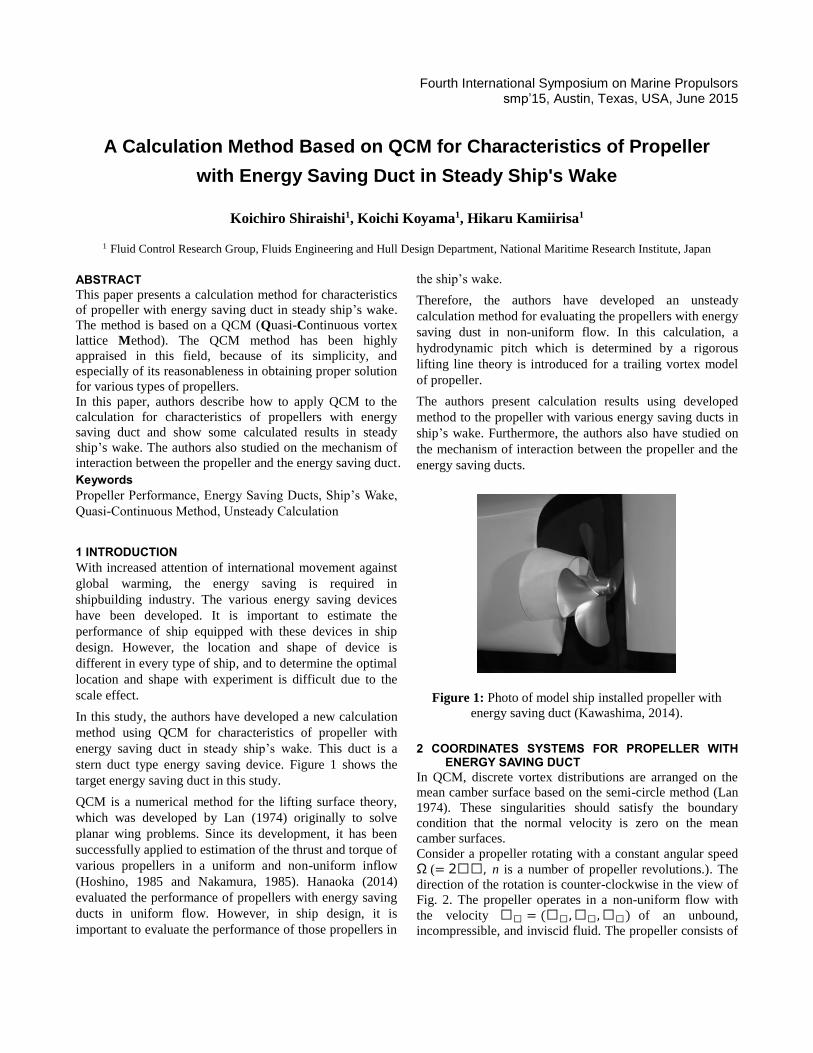
stern duct type energy saving device. Figure 1 shows the

target energy saving duct in this study.

QCM is a numerical method for the lifting surface theory,

which was developed by Lan (1974) originally to solve

planar wing problems. Since its development, it has been

successfully applied to estimation of the thrust and torque of

various propellers in a uniform and non-uniform inflow

(Hoshino, 1985 and Nakamura, 1985). Hanaoka (2014)

evaluated the performance of propellers with energy saving

ducts in uniform flow. However, in ship design, it is

important to evaluate the performance of those propellers in

the ship’s wake.

Therefore, the authors have developed an unsteady

calculation method for evaluating the propellers with energy

saving dust in non-uniform flow. In this calculation, a

hydrodynamic pitch which is determined by a rigorous

lifting line theory is introduced for a trailing vortex model

of propeller.

The authors present calculation results using developed

method to the propeller with various energy saving ducts in

ship’s wake. Furthermore, the authors also have studied on

the mechanism of interaction between the propeller and the

energy saving ducts.

Figure 1: Photo of model ship installed propeller with

energy saving duct (Kawashima, 2014).

2 COORDINATES SYSTEMS FOR PROPELLER WITH ENERGY SAVING DUCT

In QCM, discrete vortex distributions are arranged on the

mean camber surface based on the semi-circle method (Lan

1974). These singularities should satisfy the boundary

condition that the normal velocity is zero on the mean

camber surfaces.

Consider a propeller rotating with a constant angular speed

Ω (= 2𝜋𝜋, n is a number of propeller revolutions.). The

direction of the rotation is counter-clockwise in the view of

Fig. 2. The propeller operates in a non-uniform flow with

the velocity 𝜋𝜋 = (𝜋𝜋,𝜋𝜋,𝜋𝜋) of an unbound,

incompressible, and inviscid fluid. The propeller consists of

K-blades which have the same shape and are placed

symmetrically around the axis of the rotation.

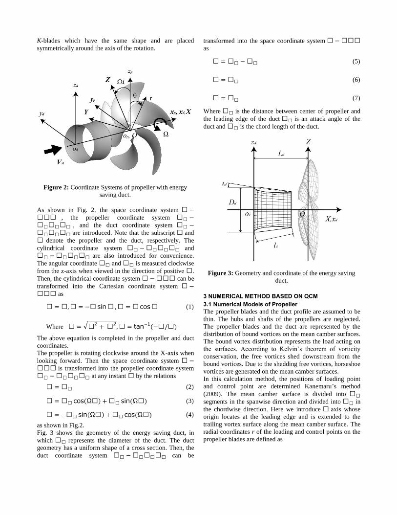
Figure 2: Coordinate Systems of propeller with energy

saving duct.

As shown in Fig. 2, the space coordinate system 𝜋 −𝜋𝜋𝜋 , the propeller coordinate system 𝜋𝜋 −𝜋𝜋𝜋𝜋𝜋𝜋 , and the duct coordinate system 𝜋𝜋 −𝜋𝜋𝜋𝜋𝜋𝜋 are introduced. Note that the subscript 𝜋 and

𝜋 denote the propeller and the duct, respectively. The

cylindrical coordinate system 𝜋𝜋 −𝜋𝜋𝜋𝜋𝜋𝜋 and

𝜋𝜋 −𝜋𝜋𝜋𝜋𝜋𝜋 are also introduced for convenience.

The angular coordinate 𝜋𝜋 and 𝜋𝜋 is measured clockwise

from the z-axis when viewed in the direction of positive 𝜋.

Then, the cylindrical coordinate system 𝜋− 𝜋𝜋𝜋 can be

transformed into the Cartesian coordinate system 𝜋 −𝜋𝜋𝜋 as

𝜋 = 𝜋,𝜋 = −𝜋 sin𝜋 ,𝜋 = 𝜋 cos𝜋 (1)

Where 𝜋 = √𝜋

2+ 𝜋

2,𝜋 = tan−1(−𝜋/𝜋)

The above equation is completed in the propeller and duct

coordinates.

The propeller is rotating clockwise around the X-axis when

looking forward. Then the space coordinate system 𝜋 −𝜋𝜋𝜋 is transformed into the propeller coordinate system

𝜋𝜋 −𝜋𝜋𝜋𝜋𝜋𝜋 at any instant 𝜋 by the relations

𝜋 = 𝜋𝜋 (2)

𝜋 = 𝜋𝜋 cos(Ω𝜋) + 𝜋𝜋 sin(Ω𝜋) (3)

𝜋 = −𝜋𝜋 sin(Ω𝜋) +𝜋𝜋 cos(Ω𝜋) (4)

as shown in Fig.2.

Fig. 3 shows the geometry of the energy saving duct, in

which 𝜋𝜋 represents the diameter of the duct. The duct

geometry has a uniform shape of a cross section. Then, the

duct coordinate system 𝜋𝜋 − 𝜋𝜋𝜋𝜋𝜋𝜋 can be

transformed into the space coordinate system 𝜋 − 𝜋𝜋𝜋

as

𝜋 = 𝜋𝜋 −𝜋𝜋 (5)

𝜋 = 𝜋𝜋 (6)

𝜋 = 𝜋𝜋 (7)

Where 𝜋𝜋 is the distance between center of propeller and

the leading edge of the duct 𝜋𝜋 is an attack angle of the

duct and 𝜋𝜋 is the chord length of the duct.

Figure 3: Geometry and coordinate of the energy saving

duct.

3 NUMERICAL METHOD BASED ON QCM

3.1 Numerical Models of Propeller

The propeller blades and the duct profile are assumed to be

thin. The hubs and shafts of the propellers are neglected.

The propeller blades and the duct are represented by the

distribution of bound vortices on the mean camber surfaces.

The bound vortex distribution represents the load acting on

the surfaces. According to Kelvin’s theorem of vorticity

conservation, the free vortices shed downstream from the

bound vortices. Due to the shedding free vortices, horseshoe

vortices are generated on the mean camber surfaces.

In this calculation method, the positions of loading point

and control point are determined Kanemaru’s method

(2009). The mean camber surface is divided into 𝜋𝜋

segments in the spanwise direction and divided into 𝜋𝜋 in

the chordwise direction. Here we introduce 𝜋 axis whose

origin locates at the leading edge and is extended to the

trailing vortex surface along the mean camber surface. The

radial coordinates r of the loading and control points on the

propeller blades are defined as

𝜋𝜋,𝜋 =

1

2(𝜋𝜋,0 + 𝜋𝜋,ℎ)

−1

2(𝜋𝜋,0

− 𝜋𝜋,ℎ) cos𝜋𝜋,𝜋

(8)

𝜋𝜋,𝜋 =

1

2(𝜋𝜋,𝜋 + 𝜋𝜋,𝜋+1) (9)

𝜋𝜋,𝜋 =

2𝜋 − 1

2(𝜋𝜋 + 1)𝜋,𝜋 = 1,2, ⋯ ,𝜋𝜋 + 1 (10)

Where 𝜋𝜋,0 and 𝜋𝜋,ℎ are the radius of the propeller and

the hub, respectively. The position of the bound vortex

𝜋𝜋,𝜋𝜋𝜋𝜋

and control point 𝜋𝜋,𝜋𝜋𝜋𝜋

on the mean camber

surface are expressed by the following equations.

𝜋𝜋,𝜋𝜋𝜋𝜋

= 𝜋𝜋,𝜋(𝜋𝜋,𝜋

)

+𝜋𝜋,𝜋(𝜋𝜋,𝜋) − 𝜋𝜋,𝜋(𝜋𝜋,𝜋)

2(1

− cos2𝜋− 1

2𝜋𝜋

𝜋)

(11)

𝜋𝜋,𝜋𝜋𝜋𝜋

= 𝜋𝜋,𝜋(𝜋𝜋,𝜋 )

+𝜋𝜋,𝜋(𝜋𝜋

) − 𝜋𝜋,𝜋(𝜋𝜋+1 )

2(1

− cos𝜋

𝜋𝜋

𝜋)

(12)

3.2 Numerical Models of Duct

In same ways of the propeller, the mean camber surface of

duct is divided into 𝜋𝜋 segments in the circumferential

direction and divided into 𝜋𝜋 in the chordwise direction.

The position of the bound vortex 𝜋𝜋,𝜋𝜋𝜋𝜋

and control point

𝜋𝜋,𝜋𝜋𝜋𝜋

on the duct mean camber surface are expressed by

the following equations.

𝜋𝜋,𝜋𝜋𝜋𝜋

= 𝜋𝜋 cosΛ (1 − cos2𝜋 − 1

2𝜋𝜋

𝜋) (13)

𝜋𝜋,𝜋𝜋𝜋𝜋

= 𝜋𝜋 cosΛ (1 − cos𝜋

𝜋𝜋

𝜋) (14)

𝜋𝜋,𝜋𝜋𝜋𝜋

= (1 − 𝜋𝜋 sinΛ) sin (2𝜋− 1

2(𝜋𝜋 + 1)𝜋)

(15)

𝜋𝜋,𝜋𝜋

𝜋𝜋= (1 − 𝜋𝜋 sinΛ) sin (

𝜋

𝜋𝜋 + 1𝜋) (16)

𝜋𝜋,𝜋𝜋𝜋𝜋

= (1 − 𝜋𝜋 sinΛ) cos (2𝜋− 1

2(𝜋𝜋 + 1)𝜋)

(17)

𝜋𝜋,𝜋𝜋

𝜋𝜋= (1 − 𝜋𝜋 sinΛ) cos (

𝜋

𝜋𝜋 + 1𝜋) (18)

3.3 Numerical Models of Trailing Vortex

The free vortices shed from the bound vortices are

considered to leave from the trailing edge and flow into the

slipstream with the local velocity at the position. In this

method, a hydrodynamic pitch which is determined by a

rigorous lifting line theory is introduced for a trailing vortex

model of propeller. This trailing vortex model has been

used by Hanaoka (1969) and Koyama (1975). The

effectiveness has been shown in their research. The

hydrodynamic pitch is expressed by the following equation

ℎ(𝜋) =𝜋 + 𝜋𝜋

Ω + 𝜋𝜋 /𝜋

(19)

Where 𝜋 is a propeller advance velocity, 𝜋𝜋 is an

averaged induced velocity in the x-axial component and

𝜋𝜋 is an averaged induced velocity in tangential

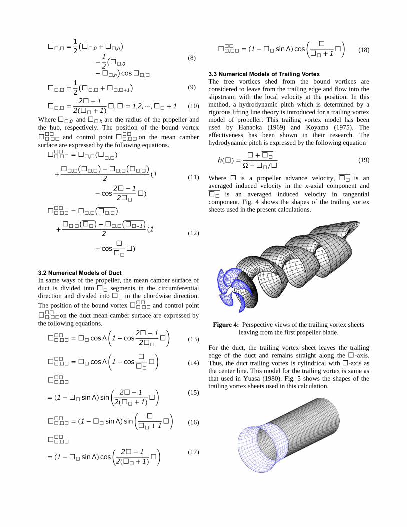
component. Fig. 4 shows the shapes of the trailing vortex

sheets used in the present calculations.

Figure 4: Perspective views of the trailing vortex sheets

leaving from the first propeller blade.

For the duct, the trailing vortex sheet leaves the trailing

edge of the duct and remains straight along the 𝜋-axis.

Thus, the duct trailing vortex is cylindrical with 𝜋-axis as

the center line. This model for the trailing vortex is same as

that used in Yuasa (1980). Fig. 5 shows the shapes of the

trailing vortex sheets used in this calculation.

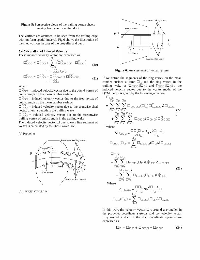
Figure 5: Perspective views of the trailing vortex sheets

leaving from energy saving duct.

The vortices are assumed to be shed from the trailing edge

with uniform spatial interval. Fig.6 shows the illustration of

the shed vortices in case of the propeller and duct.

3.4 Calculation of Induced Velocity

These induced velocity vector are expressed as

𝒗𝒗𝒗𝒗𝒗

= 𝒗𝒗𝒗𝒗𝒗

+ ∑ (𝒗𝒗𝒗+𝒗𝒗′𝒗

−𝒗𝒗𝒗𝒗′𝒗

)

𝒗𝒗

𝒗′=𝒗

− 𝒗𝒗𝒗𝒗𝒗𝒗

∣𝒗=𝒗

(20)

𝒗𝒗𝒗𝒗

𝒗= 𝒗𝒗𝒗𝒗

𝒗𝒗−𝒗𝒗𝒗𝒗+𝒗

𝒗𝒗+ 𝒗𝒗𝒗+𝒗𝒗

𝒗𝒗

− 𝒗𝒗𝒗𝒗𝒗𝒗

(21)

Where

𝒗𝒗𝒗𝒗𝒗

= induced velocity vector due to the bound vortex of

unit strength on the mean camber surface

𝒗𝒗𝒗𝒗𝒗

= induced velocity vector due to the free vortex of

unit strength on the mean camber surface

𝒗𝒗𝒗𝒗𝒗𝒗

= induced velocity vector due to the spanwise shed

vortex of unit strength in the trailing wake

𝒗𝒗𝒗𝒗𝒗𝒗

= induced velocity vector due to the streamwise

trailing vortex of unit strength in the trailing wake

The induced velocity vector 𝒗 due to each line segment of

vortex is calculated by the Biot-Savart law.

(a) Propeller

(b) Energy saving duct

Figure 6: Arrangement of vortex system

If we define the segments of the ring vortex on the mean

camber surface at time 𝜋𝜋 and the ring vortex in the

trailing wake as 𝜋𝜋𝜋𝜋(𝜋𝜋) and Γ𝜋𝜋𝜋(𝜋𝜋) , the

induced velocity vector due to the vortex model of the

QCM theory is given by the following equation.

𝒗𝜋,𝜋

= ∑ ∑ ∑ 𝜋𝜋,𝜋𝜋𝜋(𝜋𝜋)𝒗𝜋,𝜋𝜋𝜋𝜋

𝜋𝜋

𝜋=1

Δ𝜋𝜋,𝜋𝜋

𝜋𝜋

𝜋=1

𝜋𝜋

𝜋=1

(22

)

+ ∑ ∑ ∑ 𝜋𝜋,𝜋𝜋(𝜋𝜋−𝜋)𝒗𝜋,𝜋𝜋𝜋𝜋

𝜋𝜋−1

𝜋=1

𝜋𝜋

𝜋=1

𝜋𝜋

𝜋=1

Where

Δ𝜋𝜋,𝜋𝜋 =𝜋𝜋(𝜋𝜋,𝜋)

2𝜋𝜋sin

2𝜋 − 1

𝜋𝜋𝜋

𝜋𝜋,𝜋𝜋(𝜋𝜋) = ∑ 𝜋𝜋,𝜋𝜋𝜋(𝜋𝜋)Δ𝜋𝜋,𝜋𝜋

𝜋𝜋

𝜋=1

𝒗𝜋,𝜋

= ∑ ∑ 𝜋𝜋,𝜋𝜋(𝜋𝜋)𝒗𝜋,𝜋𝜋𝜋

𝜋𝜋

𝜋=1

Δ𝜋𝜋,𝜋𝜋

𝜋𝜋

𝜋=1

(23)

+ ∑ ∑ 𝜋𝜋,𝜋𝜋(𝜋𝜋−𝜋)𝒗𝜋,𝜋𝜋𝜋

𝜋𝜋−1

𝜋=1

𝜋𝜋

𝜋=1

Where

Δ𝜋𝜋,𝜋𝜋 =𝜋𝜋𝜋

2𝜋𝜋sin

2𝜋− 1

𝜋𝜋𝜋

𝜋𝜋,𝜋(𝜋𝜋) = ∑ 𝜋𝜋,𝜋𝜋(𝜋𝜋)Δ𝜋𝜋,𝜋𝜋

𝜋𝜋

𝜋=1

In this way, the velocity vector 𝒗𝒗 around a propeller in

the propeller coordinate systems and the velocity vector

𝒗𝒗 around a duct in the duct coordinate systems are

expressed as

𝒗𝜋 = 𝒗𝜋,𝜋 + 𝒗𝜋𝜋,𝜋 + 𝒗𝜋𝜋,𝜋 (24)

𝒗𝜋 = 𝒗𝜋,𝜋 + 𝒗𝜋𝜋,𝜋 + 𝒗𝜋𝜋,𝜋 (25)

Where 𝒗𝒗,𝒗 and 𝒗𝒗,𝒗 are inflow vectors of propeller

and duct respectively.

𝒗𝜋𝜋,𝜋= induced velocity vector on the propeller due to

the horseshoe vortex of the propeller.

𝒗𝜋𝜋,𝜋 = induced velocity vector on the propeller due to

the horseshoe vortex of the duct.

𝒗𝜋𝜋,𝜋= induced velocity vector on the duct due to the

horseshoe vortex of the propeller.

𝒗𝜋𝜋,𝜋= induced velocity vector on the duct due to the

horseshoe vortex of the duct.

The boundary conditions at the control points on the mean

camber surfaces of propeller and duct are that there is no

flow across the surfaces. Therefore the equation of the

boundary condition is given as follow:

𝒗𝜋 ⋅ 𝒗𝜋 = 𝒗 (26)

𝒗𝜋 ⋅ 𝒗𝜋 = 𝒗 (27)

Where 𝒗𝜋 and 𝒗𝜋 is the normal vector on the mean

camber surfaces of propeller and duct.

3.5 Calculation of Forces Acting on Propeller and Duct

Forces acting on the propeller blades and the duct can be

expressed as

𝒗 = 𝒗𝒗 +𝒗𝒗 (28)

The force 𝒗𝒗 acting on the bound vortex segments can be

calculated by Kutta-Joukowski theorem as

𝒗𝒗 = 𝒗𝒗 ⋅

𝒗

𝒗𝒗(𝒗𝒗𝒗+

𝒗− 𝒗𝒗𝒗−

𝒗) ∣ 𝒗𝒗

∣ + 𝒗𝒗𝒗 × 𝒗 (29)

Where

𝒗𝒗𝒗+𝒗

− 𝒗𝒗𝒗−𝒗

=𝜋𝜋𝜋

2𝜋∑ 𝜋𝜋𝜋

∗𝜋 (𝜋) sin𝜋𝜋

𝜋

𝜋∗

=1

where 𝒗 is the fluid density and 𝜋𝜋 is the bound vortex

segment. 𝒗𝒗 is the resultant velocity at the midpoint of a

bound vortex segment. 𝒗𝒗 is the segment vector of the

bound vortex segment. (𝒗𝒗𝒗+𝒗

−𝒗𝒗𝒗−𝒗

) means the jump

in tangential velocity across the camber surface and is equal

to the strength of the vorticity 𝜋.

The viscous drag 𝜋𝜋 can be expressed as

𝒗𝒗 =𝟏

𝟏𝒗 𝒗𝒗𝒗𝒗

|𝒗𝒗||𝒗𝒗| (30)

The viscous drag coefficient 𝜋𝜋 is calculated empirically

as (Nakamura, 1985).

The thrusts and torque acting on the propeller and duct are

calculated by

𝜋 = ∑𝜋𝜋𝜋

2𝜋𝜋

𝜋𝜋𝜋 sin𝜋𝜋

𝜋

𝜋=1

(31)

𝜋 = ∑

𝜋𝜋𝜋

2𝜋𝜋

(𝜋𝜋𝜋𝜋𝜋

𝜋

𝜋=1

− 𝜋𝜋𝜋𝜋𝜋) sin𝜋𝜋

(32)

The thrust coefficients 𝜋𝜋,𝜋 and 𝜋𝜋,𝜋 of the propeller

and the duct and the total thrust coefficient 𝜋𝜋 are defined

by

𝜋𝜋,𝜋 =𝜋𝜋

𝜋𝜋2𝜋𝜋

4 (33)

𝜋𝜋,𝜋 =

𝜋𝜋

𝜋𝜋2𝜋𝜋

4 (34)

𝜋𝜋 =

𝜋𝜋 + 𝜋𝜋

𝜋𝜋2𝜋𝜋

4= 𝜋𝜋,𝜋 +𝜋𝜋,𝜋 (35)

Where 𝜋 = Ω/(2π) is the number of propeller rotation.

Similarly, the torque coefficient 𝜋𝜋 and 𝜋 of the propeller

are defined by

𝜋𝜋 =

𝜋

𝜋𝜋2𝜋𝜋

5 (36)

𝜋 =

𝜋𝜋𝜋

2𝜋𝜋𝜋

(37)

4 CALCULATION

The authors select highly skewed propeller (HSP) of Seiun-

Maru-I in order to verify the present calculation compare

the Hoshino’s calculation results using panel method

(Hoshino 1998a). Furthermore, the authors evaluated the

propeller performance with various energy saving ducts in

wake of Seiun-Maru-I to study on the mechanism of the

energy saving ducts.

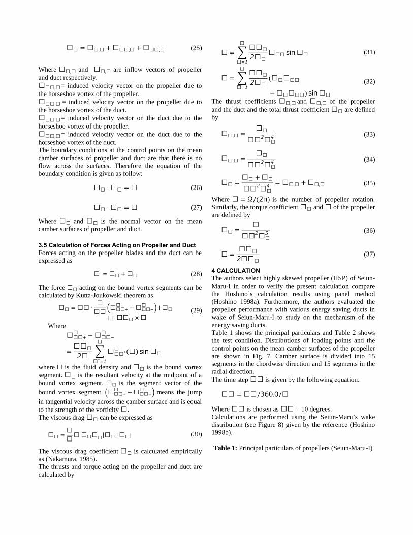
Table 1 shows the principal particulars and Table 2 shows

the test condition. Distributions of loading points and the

control points on the mean camber surfaces of the propeller

are shown in Fig. 7. Camber surface is divided into 15

segments in the chordwise direction and 15 segments in the

radial direction.

The time step 𝜋𝜋 is given by the following equation.

𝜋𝜋 = 𝜋𝜋/360.0/𝜋

Where 𝜋𝜋 is chosen as 𝜋𝜋 = 10 degrees.

Calculations are performed using the Seiun-Maru’s wake

distribution (see Figure 8) given by the reference (Hoshino

1998b).

Table 1: Principal particulars of propellers (Seiun-Maru-I)

Name of Propeller HSP

Diameter (m) 3.600

Number of Blade 5

Pitch Ratio at 0.7R 0.944

Expanded are Ratio 0.7

Hub Ratio 0.1972

Rake Angle (deg.) -3.03

Blade Section Modified SRI-B

Table 2: Test Condition

𝜋, Ship Speed (knots) 9.0

𝜋, Rotation Speed (rpm) 90.7

𝜋 = 𝜋/𝜋𝜋 0.851

Figure 7: Distributions of the horseshoe vortices (blue

lines) and the control points (red points) on the mean

camber surfaces of the propeller.

Figure 8: Wake velocity distribution of Seiun-Maru-I

4.1 Verification of Present Calculation on Propeller without Duct

Fig. 9 shows the calculated thrust and torque fluctuations

acting on one blade of HSP comparing with the results of

Hoshino’s panel method (Hoshino, 1998b). It is found that

the calculated results agree well with the Hoshino’s results

except for the angular position around Θ = 0 degree.

Figure 9: Comparison of thrust and torque coefficients

fluctuation.

4.2 Study on Mechanism of Energy Saving Duct

In order to investigate the mechanism of energy saving

ducts, the authors evaluated the propeller characteristics

with the energy saving duct in uniform flow. Furthermore, 4

types of duct are evaluated in Seiun-Maru’s wake. Table 3

shows the principal particulars of the energy saving ducts.

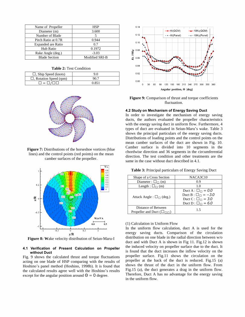
Distributions of loading points and the control points on the

mean camber surfaces of the duct are shown in Fig. 10.

Camber surface is divided into 10 segments in the

chordwise direction and 36 segments in the circumferential

direction. The test condition and other treatments are the

same in the case without duct described in 4.1.

Table 3: Principal particulars of Energy Saving Duct

Shape of a Cross Section NACA3C10

Diameter : 𝜋𝜋 (m) 0.9

Length : 𝜋𝜋 (m) 1.0

Attack Angle : 𝜋𝜋 (deg.)

Duct A : 𝜋𝜋 = 0.0 Duct B : 𝜋𝜋 = −3.0

Duct C : 𝜋𝜋 = 3.0 Duct D : 𝜋𝜋 = 6.0

Distance of Between

Propeller and Duct (𝜋𝜋𝜋) 1.5

(1) Calculation in Uniform Flow

In the uniform flow calculation, duct A is used for the

energy saving ducts. Comparison of the circulation

distribution on one blade in the radial direction between w/o

duct and with Duct A is shown in Fig 11. Fig.12 is shown

the induced velocity on propeller surface due to the duct. It

is found that the duct increases the inflow velocity on the

propeller surface. Fig.11 shows the circulation on the

propeller at the back of the duct is reduced. Fig.15 (a)

shows the thrust of the duct in the uniform flow. From

Fig.15 (a), the duct generates a drag in the uniform flow.

Therefore, Duct A has no advantage for the energy saving

in the uniform flow.

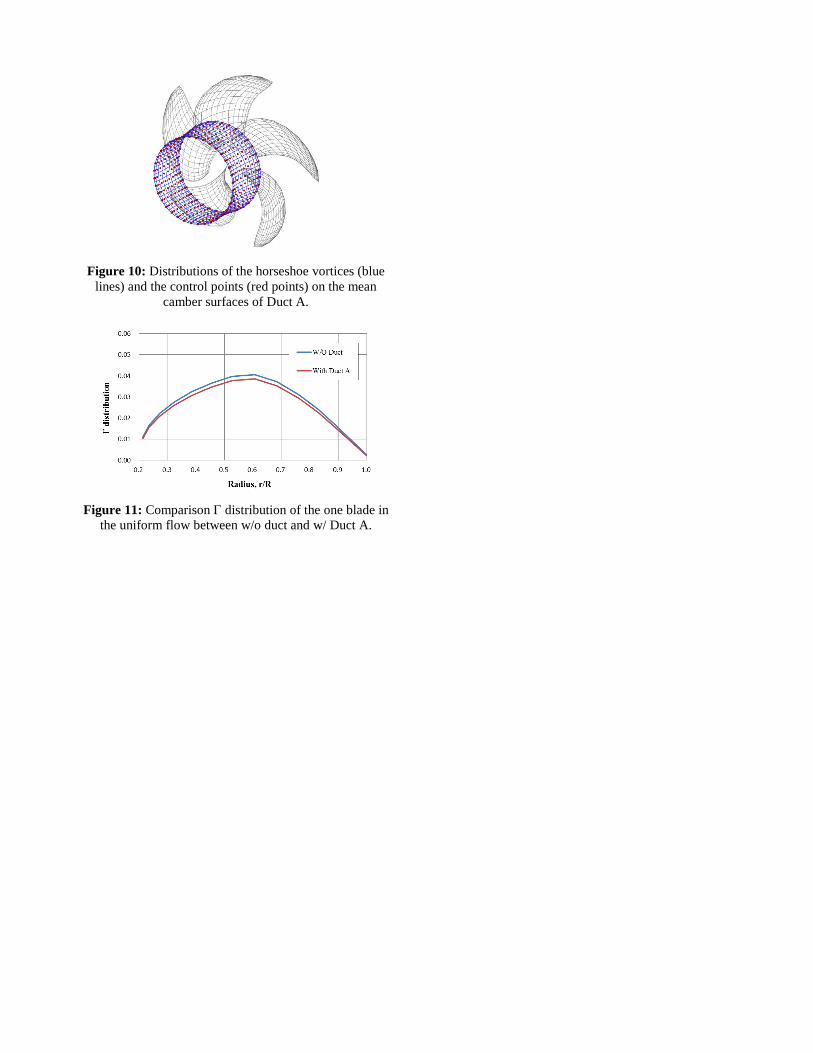
Figure 10: Distributions of the horseshoe vortices (blue

lines) and the control points (red points) on the mean

camber surfaces of Duct A.

Figure 11: Comparison distribution of the one blade in

the uniform flow between w/o duct and w/ Duct A.

(a) Axial velocity

(b) Radial velocity

(c) Tangential velocity

Figure 12: Comparison of induced velocity of propeller due to Duct A in the uniform flow.

Dashed circles show the position of leading edge of duct.

(a) Axial velocity

(b) Radial velocity

(c) Tangential velocity

Figure 13: Comparison of induced velocity of propeller due to Duct A in the Seiun-Maru’s wake.

Dashed circles show the position of leading edge of duct.

(a) 0.3R

(b) 0.4R

(c) 0.5R

(d) 0.6R

(e) 0.7R

(f) 0.8R

Figure 14: Comparison of distribution on one blade in the Seiun-Maru’s wake between w/o duct and w/ Duct A.

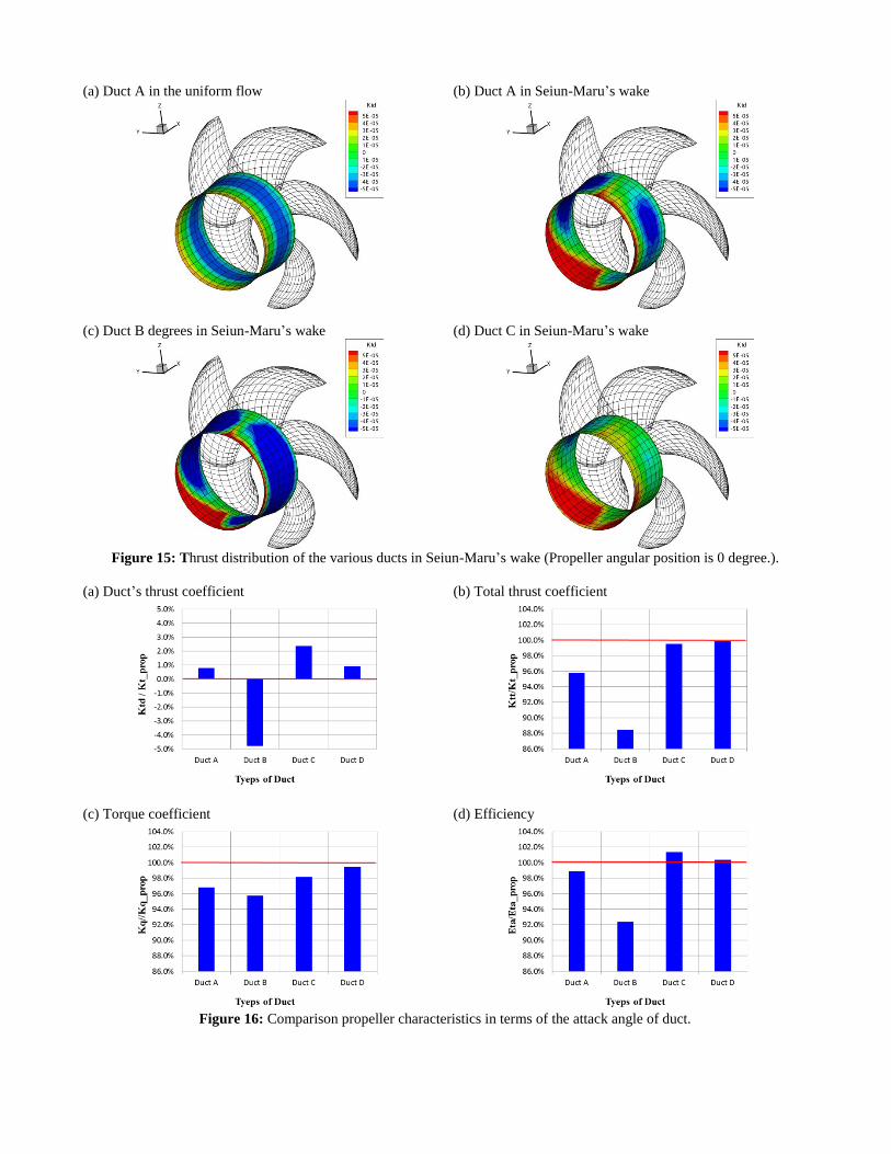
(a) Duct A in the uniform flow (b) Duct A in Seiun-Maru’s wake

(c) Duct B degrees in Seiun-Maru’s wake (d) Duct C in Seiun-Maru’s wake

Figure 15: Thrust distribution of the various ducts in Seiun-Maru’s wake (Propeller angular position is 0 degree.).

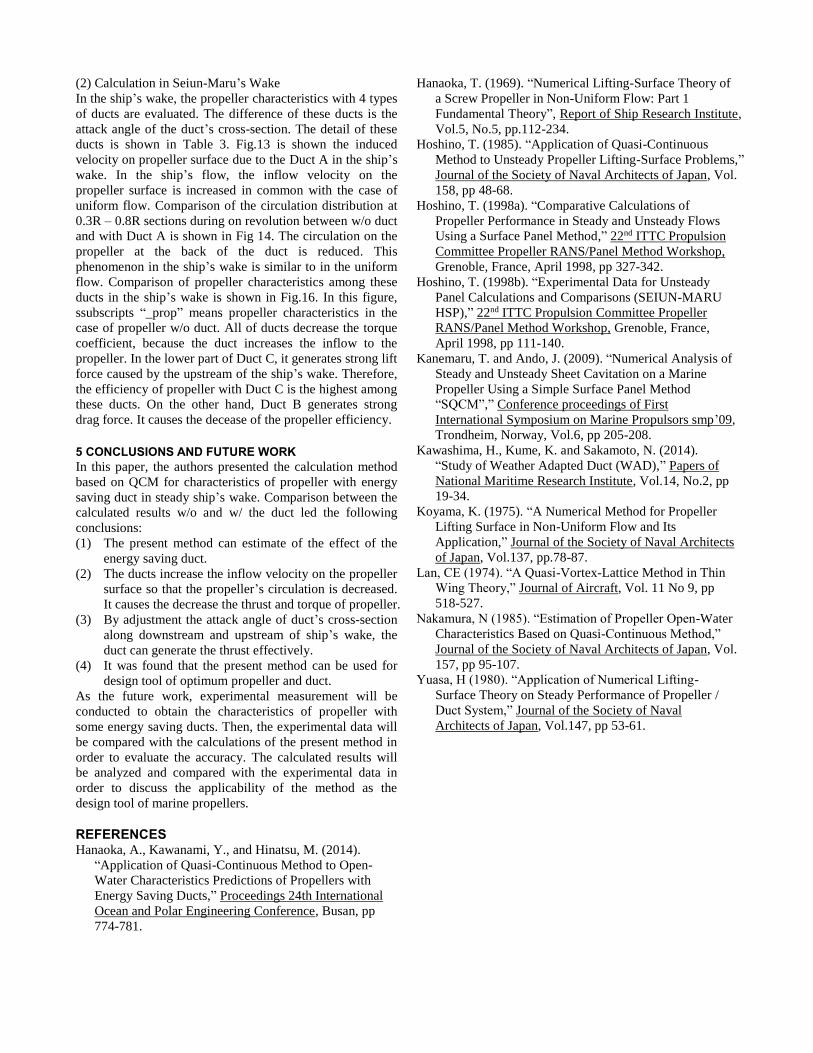
(a) Duct’s thrust coefficient (b) Total thrust coefficient

(c) Torque coefficient (d) Efficiency

Figure 16: Comparison propeller characteristics in terms of the attack angle of duct.

(2) Calculation in Seiun-Maru’s Wake

In the ship’s wake, the propeller characteristics with 4 types

of ducts are evaluated. The difference of these ducts is the

attack angle of the duct’s cross-section. The detail of these

ducts is shown in Table 3. Fig.13 is shown the induced

velocity on propeller surface due to the Duct A in the ship’s

wake. In the ship’s flow, the inflow velocity on the

propeller surface is increased in common with the case of

uniform flow. Comparison of the circulation distribution at

0.3R – 0.8R sections during on revolution between w/o duct

and with Duct A is shown in Fig 14. The circulation on the

propeller at the back of the duct is reduced. This

phenomenon in the ship’s wake is similar to in the uniform

flow. Comparison of propeller characteristics among these

ducts in the ship’s wake is shown in Fig.16. In this figure,

ssubscripts “_prop” means propeller characteristics in the

case of propeller w/o duct. All of ducts decrease the torque

coefficient, because the duct increases the inflow to the

propeller. In the lower part of Duct C, it generates strong lift

force caused by the upstream of the ship’s wake. Therefore,

the efficiency of propeller with Duct C is the highest among

these ducts. On the other hand, Duct B generates strong

drag force. It causes the decease of the propeller efficiency.

5 CONCLUSIONS AND FUTURE WORK

In this paper, the authors presented the calculation method

based on QCM for characteristics of propeller with energy

saving duct in steady ship’s wake. Comparison between the

calculated results w/o and w/ the duct led the following

conclusions:

(1) The present method can estimate of the effect of the

energy saving duct.

(2) The ducts increase the inflow velocity on the propeller

surface so that the propeller’s circulation is decreased.

It causes the decrease the thrust and torque of propeller.

(3) By adjustment the attack angle of duct’s cross-section

along downstream and upstream of ship’s wake, the

duct can generate the thrust effectively.

(4) It was found that the present method can be used for

design tool of optimum propeller and duct.

As the future work, experimental measurement will be

conducted to obtain the characteristics of propeller with

some energy saving ducts. Then, the experimental data will

be compared with the calculations of the present method in

order to evaluate the accuracy. The calculated results will

be analyzed and compared with the experimental data in

order to discuss the applicability of the method as the

design tool of marine propellers.

REFERENCES Hanaoka, A., Kawanami, Y., and Hinatsu, M. (2014).

“Application of Quasi-Continuous Method to Open-

Water Characteristics Predictions of Propellers with

Energy Saving Ducts,” Proceedings 24th International

Ocean and Polar Engineering Conference, Busan, pp

774-781.

Hanaoka, T. (1969). “Numerical Lifting-Surface Theory of

a Screw Propeller in Non-Uniform Flow: Part 1

Fundamental Theory”, Report of Ship Research Institute,

Vol.5, No.5, pp.112-234.

Hoshino, T. (1985). “Application of Quasi-Continuous

Method to Unsteady Propeller Lifting-Surface Problems,”

Journal of the Society of Naval Architects of Japan, Vol.

158, pp 48-68.

Hoshino, T. (1998a). “Comparative Calculations of

Propeller Performance in Steady and Unsteady Flows

Using a Surface Panel Method,” 22nd ITTC Propulsion

Committee Propeller RANS/Panel Method Workshop,

Grenoble, France, April 1998, pp 327-342.

Hoshino, T. (1998b). “Experimental Data for Unsteady

Panel Calculations and Comparisons (SEIUN-MARU

HSP),” 22nd ITTC Propulsion Committee Propeller

RANS/Panel Method Workshop, Grenoble, France,

April 1998, pp 111-140.

Kanemaru, T. and Ando, J. (2009). “Numerical Analysis of

Steady and Unsteady Sheet Cavitation on a Marine

Propeller Using a Simple Surface Panel Method

“SQCM”,” Conference proceedings of First

International Symposium on Marine Propulsors smp’09,

Trondheim, Norway, Vol.6, pp 205-208.

Kawashima, H., Kume, K. and Sakamoto, N. (2014).

“Study of Weather Adapted Duct (WAD),” Papers of

National Maritime Research Institute, Vol.14, No.2, pp

19-34.

Koyama, K. (1975). “A Numerical Method for Propeller

Lifting Surface in Non-Uniform Flow and Its

Application,” Journal of the Society of Naval Architects

of Japan, Vol.137, pp.78-87.

Lan, CE (1974). “A Quasi-Vortex-Lattice Method in Thin

Wing Theory,” Journal of Aircraft, Vol. 11 No 9, pp

518-527.

Nakamura, N (1985). “Estimation of Propeller Open-Water

Characteristics Based on Quasi-Continuous Method,”

Journal of the Society of Naval Architects of Japan, Vol.

157, pp 95-107.

Yuasa, H (1980). “Application of Numerical Lifting-

Surface Theory on Steady Performance of Propeller /

Duct System,” Journal of the Society of Naval

Architects of Japan, Vol.147, pp 53-61.

DISCUSSION

Question from Tom van Terwisga

Can you say something on the comparison of the duct

effectiveness before open water condition and the condition

behind the Seiun-maru?

Authors’ Closure

Thank you for your insightful comment. We haven’t

compared the duct effectiveness before open water

condition and the condition behind the wake. However, the

effect of the duct in uniform flow has been examined. In the

uniform flow, the duct generates drag and increases the

flow inside of itself. It causes the decease of the propeller

efficiency.

We agree that additional calculation as you suggested

would be valuable. As the future work, the comparison

calculation will be conducted.