A brief introduction toConditional Random Fields

Mark Johnson

Macquarie University

April, 2005, updated October 2010

1

Talk outline

• Graphical models

• Maximum likelihood and maximum conditional likelihood

estimation

• Naive Bayes and Maximum Entropy Models

• Hidden Markov Models

• Conditional Random Fields

2

Classification with structured labels

• Classification: predicting label y given features x

y⋆(x) = arg maxy

P(y|x)

• Naive Bayes and Maxent models: label y is atomic, x can be

structured (e.g., set of features)

• HMMs and CRFs are extensions of Naive Bayes and Maxent

models where y is structured too

• HMMs and CRFs model dependencies between components yi

of label y

• Example: Part of speech tagging: x is a sequence of words, y is

corresponding sequence of parts of speech (e.g., noun, verb,

etc.)

3

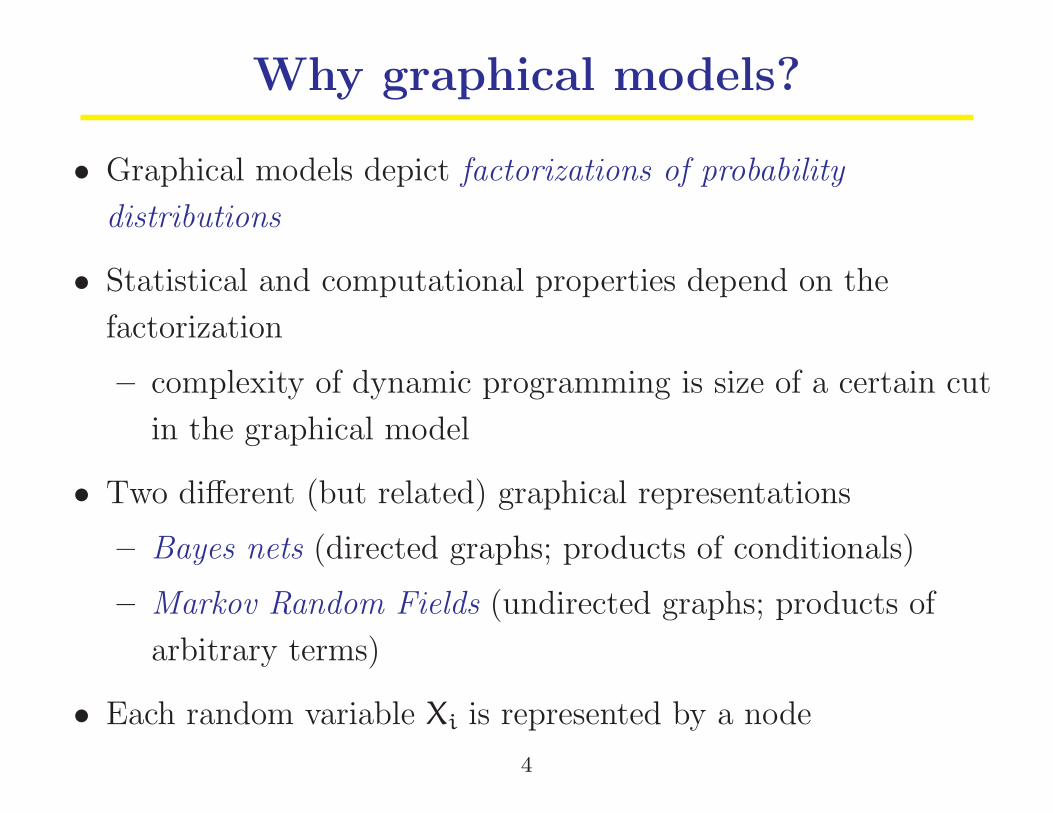
Why graphical models?

• Graphical models depict factorizations of probability

distributions

• Statistical and computational properties depend on the

factorization

– complexity of dynamic programming is size of a certain cut

in the graphical model

• Two different (but related) graphical representations

– Bayes nets (directed graphs; products of conditionals)

– Markov Random Fields (undirected graphs; products of

arbitrary terms)

• Each random variable Xi is represented by a node

4

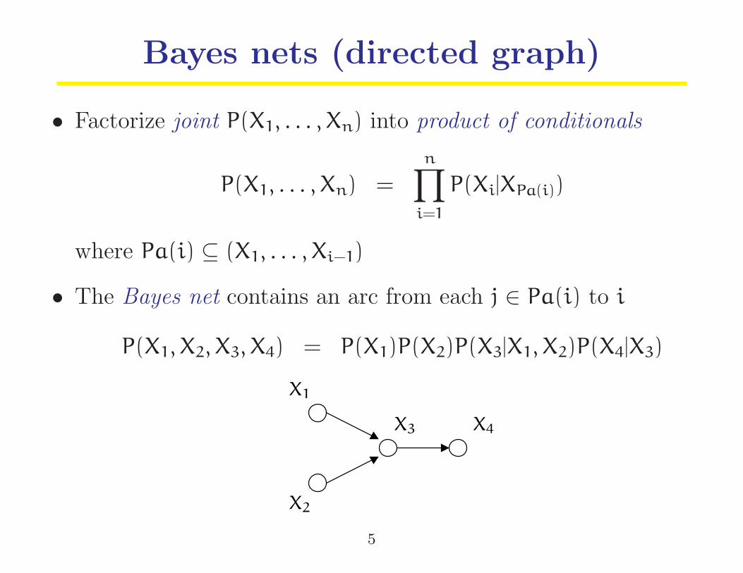
Bayes nets (directed graph)

• Factorize joint P(X1, . . . , Xn) into product of conditionals

P(X1, . . . , Xn) =

n∏

i=1

P(Xi|XPa(i))

where Pa(i) ⊆ (X1, . . . , Xi−1)

• The Bayes net contains an arc from each j ∈ Pa(i) to i

P(X1, X2, X3, X4) = P(X1)P(X2)P(X3|X1, X2)P(X4|X3)

X1

X2

X3 X4

5

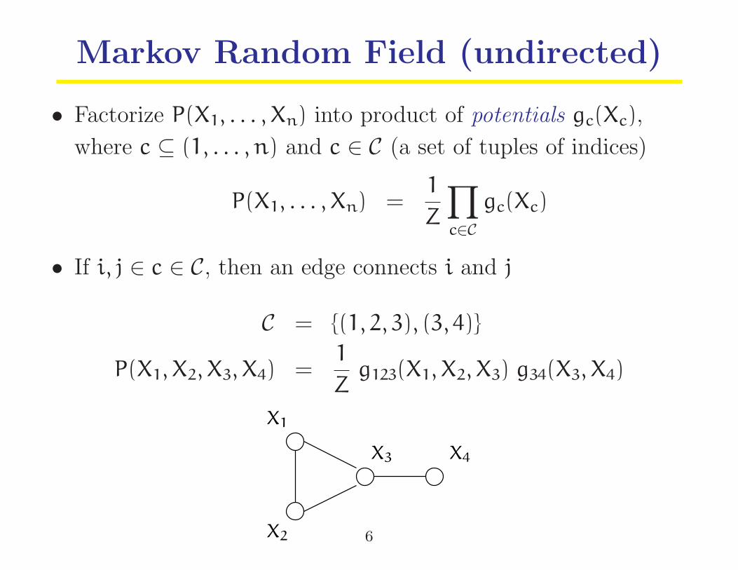
Markov Random Field (undirected)

• Factorize P(X1, . . . , Xn) into product of potentials gc(Xc),

where c ⊆ (1, . . . , n) and c ∈ C (a set of tuples of indices)

P(X1, . . . , Xn) =1

Z

∏

c∈C

gc(Xc)

• If i, j ∈ c ∈ C, then an edge connects i and j

C = {(1, 2, 3), (3, 4)}

P(X1, X2, X3, X4) =1

Zg123(X1, X2, X3) g34(X3, X4)

X1

X2

X3 X4

6

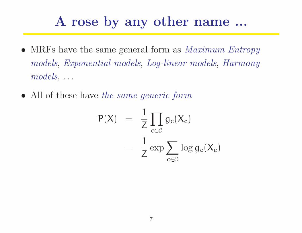
A rose by any other name ...

• MRFs have the same general form as Maximum Entropy

models, Exponential models, Log-linear models, Harmony

models, . . .

• All of these have the same generic form

P(X) =1

Z

∏

c∈C

gc(Xc)

=1

Zexp

∑

c∈C

log gc(Xc)

7

Potential functions as features

• If X is discrete, we can represent the potentials gc(Xc) as a

combination of indicator functions [[Xc = xc]], where Xc is the

set of all possible values of Xc

gc(Xc) =∏

xc∈Xc

(θXc=xc)[[Xc=xc]], where θXc=xc

= gc(xc)

log gc(Xc) =∑

xc∈Xc

[[Xc = xc]]φXc=xc, where φXc=xc

= log gc(xc)

• View [[Xc = xc]] as a feature which “fires” when the

configuration xc occurs

• φXc=xcis the weight associated with feature [[Xc = xc]]

8

A feature-based reformulation of MRFs

• Reformulating MRFs as features:

P(X) =1

Z

∏

c∈C

gc(Xc)

=1

Z

∏

c∈C,xc∈Xc

(θXc=xc)[[Xc=xc]], where θXc=xc

= gc(xc)

=1

Zexp

∑

c∈C,Xc∈Xc

[[Xc = xc]]φXc=xc, where φXc=xc

= log gc(xc)

P(X) =1

Zg123(X1, X2, X3) g34(X3, X4)

=1

Zexp

[[X123 = 000]]φ000 + [[X123 = 001]]φ001 + . . .

[[X34 = 00]]φ00 + [[X34 = 01]]φ01 + . . .

9

Bayes nets and MRFs

• MRFs are more general than Bayes nets

• Its easy to find the MRF representation of a Bayes net

P(X1, X2, X3, X4) = P(X1)P(X2)P(X3|X1, X2)︸ ︷︷ ︸g123(X1, X2, X3)

P(X4|X3)︸ ︷︷ ︸g34(X3, X4)

• Moralization, i.e, “marry the parents”

X1

X2

X3 X4

X1

X2

X3 X4

10

Conditionalization in MRFs

• Conditionalization is fixing the value of some variables

• To get a MRF representation of the conditional distribution,

delete nodes whose values are fixed and arcs connected to them

P(X1, X2, X4|X3 = v) =1

Z P(X3 = v)g123(X1, X2, v) g34(v, X4)

=1

Z ′(v)g ′

12(X1, X2) g ′

4(X4)

X1

X2

X3 = v X4

X1

X2

X4

11

Classification

• Given value of X, predict value of Y

• Given a probabilistic model P(Y|X), predict:

y⋆(x) = arg maxy

P(y|x)

• In general we must learn P(Y|X) from data

D = ((x1, y1), . . . , (xn, yn))

• Restrict attention to a parametric model class Pθ parameterized

by parameter vector θ

– learning is estimating θ from D

12

ML and CML Estimation

• Maximum likelihood estimation (MLE) picks the θ that makes

the data D = (x, y) as likely as possible

θ̂ = arg maxθ

Pθ(x, y)

• Conditional maximum likelihood estimation (CMLE) picks the

θ that maximizes conditional likelihood of the data D = (x, y)

^̂θ = arg maxθ

Pθ(y|x)

• P(X, Y) = P(X)P(Y|X), so CMLE ignores P(X)

13

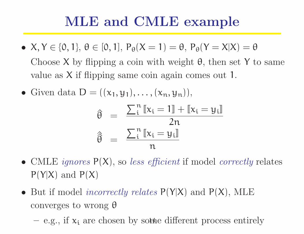
MLE and CMLE example

• X, Y ∈ {0, 1}, θ ∈ [0, 1], Pθ(X = 1) = θ, Pθ(Y = X|X) = θ

Choose X by flipping a coin with weight θ, then set Y to same

value as X if flipping same coin again comes out 1.

• Given data D = ((x1, y1), . . . , (xn, yn)),

θ̂ =

∑n

i [[xi = 1]] + [[xi = yi]]

2n

^̂θ =

∑n

i [[xi = yi]]

n

• CMLE ignores P(X), so less efficient if model correctly relates

P(Y|X) and P(X)

• But if model incorrectly relates P(Y|X) and P(X), MLE

converges to wrong θ

– e.g., if xi are chosen by some different process entirely14

Complexity of decoding and estimation

• Finding y⋆(x) = arg maxy P(y|x) is equally hard for Bayes nets

and MRFs with similar architectures

• A Bayes net is a product of independent conditional

probabilities

⇒ MLE is relative frequency (easy to compute)

– no closed form for CMLE if conditioning variables have

parents

• A MRF is a product of arbitrary potential functions g

– estimation involves learning values of each g takes

– partition function Z changes as we adjust g

⇒ usually no closed form for MLE and CMLE

15

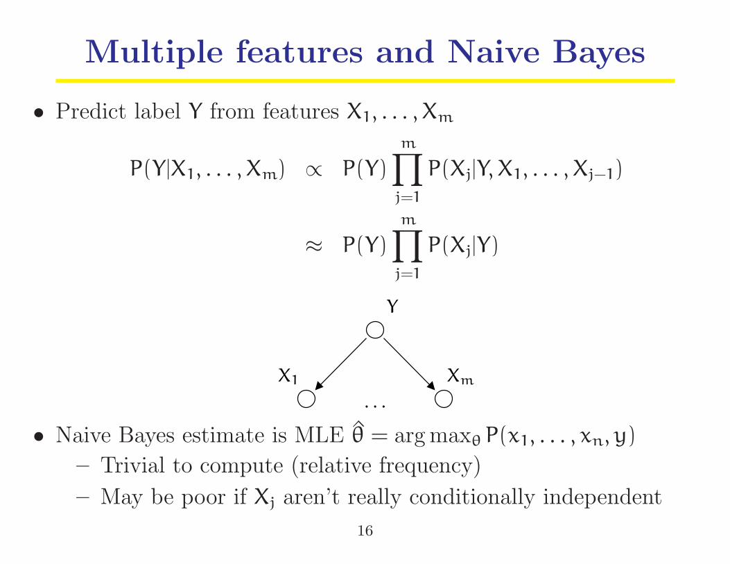
Multiple features and Naive Bayes

• Predict label Y from features X1, . . . , Xm

P(Y|X1, . . . , Xm) ∝ P(Y)

m∏

j=1

P(Xj|Y, X1, . . . , Xj−1)

≈ P(Y)

m∏

j=1

P(Xj|Y)

X1 Xm

Y

. . .

• Naive Bayes estimate is MLE θ̂ = arg maxθ P(x1, . . . , xn, y)

– Trivial to compute (relative frequency)

– May be poor if Xj aren’t really conditionally independent

16

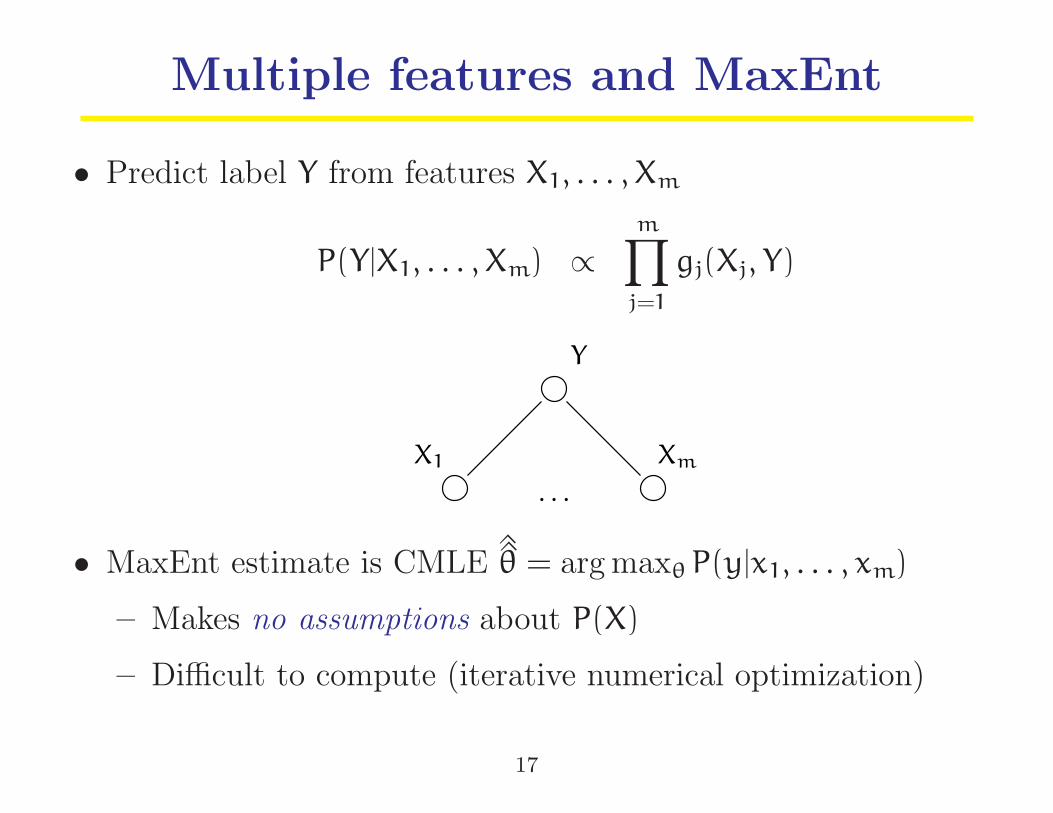
Multiple features and MaxEnt

• Predict label Y from features X1, . . . , Xm

P(Y|X1, . . . , Xm) ∝

m∏

j=1

gj(Xj, Y)

X1 Xm

Y

. . .

• MaxEnt estimate is CMLE ^̂θ = arg maxθ P(y|x1, . . . , xm)

– Makes no assumptions about P(X)

– Difficult to compute (iterative numerical optimization)

17

Sequence labeling

• Predict labels Y1, . . . , Ym given features X1, . . . , Xm

• Example: Parts of speech

Y = DT JJ NN VBS JJR

X = the big dog barks loudly

• Example: Named entities

Y = [NP NP NP] − −

X = the big dog barks loudly

• Example: X1, . . . , Xm are image regions, each Xj is labeled Yj

18

Hidden Markov Models

P(X, Y) =

m∏

j=1

P(Yj|Yj−1)P(Xj|Yj)

P(Ym, stop)

X1 X2 Xm

Y1 Y2 Ym Ym+1Y0

. . .

. . .

• Usually assume time invariance or stationarity

i.e., P(Yj|Yj−1) and P(Xj|Yj) do not depend on j

• HMMs are Naive Bayes models with compound labels Y

• Estimator is MLE θ̂ = arg maxθ Pθ(x, y)

19

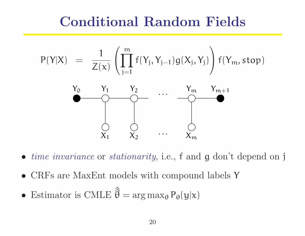
Conditional Random Fields

P(Y|X) =1

Z(x)

m∏

j=1

f(Yj, Yj−1)g(Xj, Yj)

f(Ym, stop)

X1 X2 Xm

Y1 Y2 Ym Ym+1Y0

. . .

. . .

• time invariance or stationarity, i.e., f and g don’t depend on j

• CRFs are MaxEnt models with compound labels Y

• Estimator is CMLE ^̂θ = arg maxθ Pθ(y|x)

20

Decoding and Estimation

• HMMs and CRFs have same complexity of decoding i.e.,

computing y⋆(x) = arg maxy P(y|x)

– dynamic programming algorithm (Viterbi algorithm)

• Estimating a HMM from labeled data (x, y) is trivial

– HMMs are Bayes nets ⇒ MLE is relative frequency

• Estimating a CRF from labeled data (x, y) is difficult

– Usually no closed form for partition function Z(x)

– Use iterative numerical optimization procedures (e.g.,

Conjugate Gradient, Limited Memory Variable Metric) to

maximize Pθ(y|x)

21

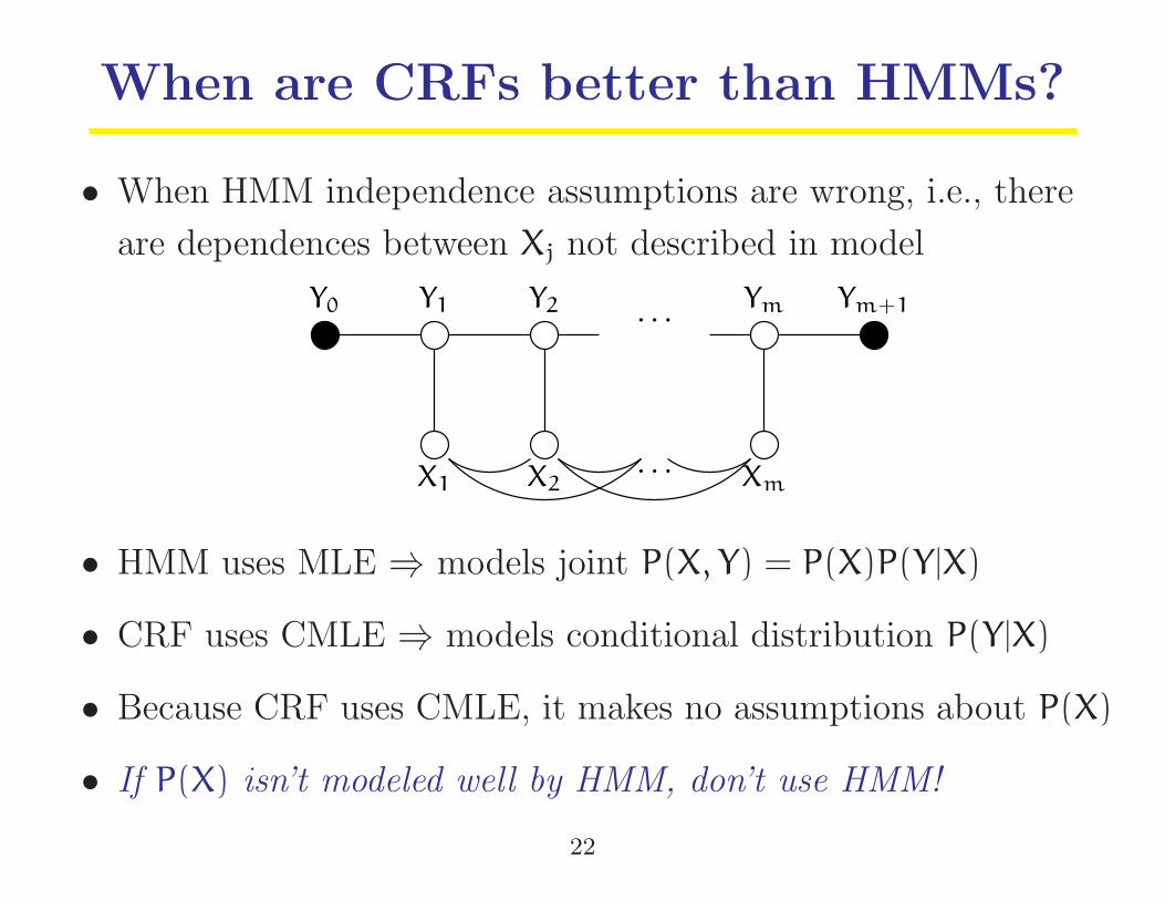
When are CRFs better than HMMs?

• When HMM independence assumptions are wrong, i.e., there

are dependences between Xj not described in model

X1 X2 Xm

Y1 Y2 Ym Ym+1Y0

. . .

. . .

• HMM uses MLE ⇒ models joint P(X, Y) = P(X)P(Y|X)

• CRF uses CMLE ⇒ models conditional distribution P(Y|X)

• Because CRF uses CMLE, it makes no assumptions about P(X)

• If P(X) isn’t modeled well by HMM, don’t use HMM!

22

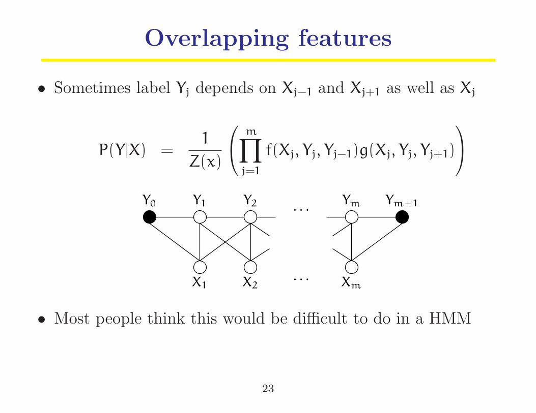
Overlapping features

• Sometimes label Yj depends on Xj−1 and Xj+1 as well as Xj

P(Y|X) =1

Z(x)

m∏

j=1

f(Xj, Yj, Yj−1)g(Xj, Yj, Yj+1)

X1 X2 Xm

Y1 Y2 Ym Ym+1Y0

. . .

. . .

• Most people think this would be difficult to do in a HMM

23

Summary

• HMMs and CRFs both associate a sequence of labels (Y1, . . . , Ym)

to items (X1, . . . , Xm)

• HMMs are Bayes nets and estimated by MLE

• CRFs are MRFs and estimated by CMLE

• HMMs assume that Xj are conditionally independent

• CRFs do not assume that the Xj are conditionally independent

• The Viterbi algorithm computes y⋆(x) for both HMMs and CRFs

• HMMs are trivial to estimate

• CRFs are difficult to estimate

• It is easier to add new features to a CRF

• There is no EM version of CRF

24

HMM with longer range dependencies

X1 X2 Xm

Y1 Y2 Ym Ym+1Y0

. . .

. . .

25