A Brief DPL Tutorial When you first start DPL you get a four pane window: Project Manager, Session Log windows on the left, and the two Model windows on the right. (Figure 1)

Figure 1

As for now, ignore the Project Manager and the Session Log windows. Maximize the Model window so that your screen looks like in Figure 2. The upper pane is where you build the Influence Diagram and the lower pane is for the Decision Tree. Only one pane is active at each time.

Figure 2

1

Policy Tree You begin creating your DPL model by inputting data in the Influence Diagram Pane, and then perfecting your model by adding and adjusting it in the Decision Tree Pane. After your decision tree is completed, you can run your analysis (“Analysis/Decision Analysis”) and DPL will create a graphical display of your model – a Policy Tree. What the Policy Tree does:

♦ Shows the result of your analysis by explicitly displaying every path of the tree. ♦ Fills in the probabilities for each chance event. ♦ Evaluates the Outcome expressions and displays their value under each branch. ♦ Evaluates and displays the Objective Function value in brackets above each

endpoint. ♦ Evaluates and displays the Expected Value of each node, just to the left of each

node, in brackets.

Objective Function Value

Get/Pay Value

Expected Value of this node

Probability

Figure 3

We will now do a simple example, where there are no uncertainties and we will ignore the time value of money. You may want to have your copy of DPL up and running on your computer in order to be able to replicate the steps in the examples.

2

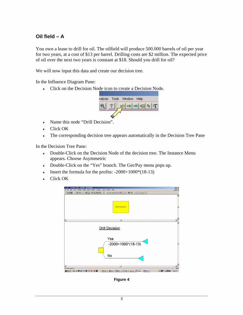
Oil field – A You own a lease to drill for oil. The oilfield will produce 500.000 barrels of oil per year for two years, at a cost of $13 per barrel. Drilling costs are $2 million. The expected price of oil over the next two years is constant at $18. Should you drill for oil? We will now input this data and create our decision tree. In the Influence Diagram Pane:

♦ Click on the Decision Node icon to create a Decision Node.

♦ Name this node “Drill Decision”. ♦ Click OK ♦ The corresponding decision tree appears automatically in the Decision Tree Pane

In the Decision Tree Pane:

♦ Double-Click on the Decision Node of the decision tree. The Instance Menu appears. Choose Asymmetric

♦ Double-Click on the “Yes” branch. The Get/Pay menu pops up. ♦ Insert the formula for the profits: -2000+1000*(18-13) ♦ Click OK

Figure 4

3

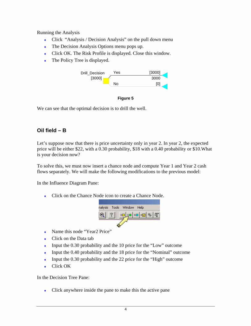
Running the Analysis ♦ Click “Analysis / Decision Analysis” on the pull down menu ♦ The Decision Analysis Options menu pops up. ♦ Click OK. The Risk Profile is displayed. Close this window. ♦ The Policy Tree is displayed.

Yes

3000 [3000]

No [0]

Drill_Decision [3000]

Figure 5

We can see that the optimal decision is to drill the well.

Oil field – B Let’s suppose now that there is price uncertainty only in year 2. In year 2, the expected price will be either $22, with a 0.30 probability, $18 with a 0.40 probability or $10.What is your decision now? To solve this, we must now insert a chance node and compute Year 1 and Year 2 cash flows separately. We will make the following modifications to the previous model: In the Influence Diagram Pane:

♦ Click on the Chance Node icon to create a Chance Node.

♦ Name this node “Year2 Price” ♦ Click on the Data tab ♦ Input the 0.30 probability and the 10 price for the “Low” outcome ♦ Input the 0.40 probability and the 18 price for the “Nominal” outcome ♦ Input the 0.30 probability and the 22 price for the “High” outcome ♦ Click OK

In the Decision Tree Pane:

♦ Click anywhere inside the pane to make this the active pane

4

♦ Click on “Node / Add Chance” in the pull down menu. ♦ Choose “Year2 Price” ♦ Attach this chance node to the upper branch of the “Drill Decision” node

anch of

♦

y branch of the “Year2_Price” node. The Get/Pay menu pops up.

♦ Separate the Year 1 and Year 2 production. Double-Click on the “Yes” brthe “Drill Decision” node. The Get/Pay menu pops up. Change the formula there to: -2000+500*(18-13)

♦ Click OK ♦ Click on an♦ Input the Year 2 cash flow formula: 500*(Year2_Price – 13). You can use the

Variable Icon button in the Get/Pay menu to input the Year2 Price variableinstead of typing it in.

t this point, your screen should look like Figure 6: A

Figure 6

After running the analysis, the policy tree shown in Figure 7:

Year2_Price

Yes 500

[2400]

No [0]

Drill_Decision [2400]

Figure 7

5

You can double-click on the Year2_Price chance node to expand the branches. After

sizing, the Policy Tree will now look like Figure 8:

Low -1500 .300 [-1000]

re

Nominal 2500 .400

[3000]

High 4500 .300

[5000]

Year2_Price Yes

500 [2400]

No [0]

Drill_Decision [2400]

Figure 8

It is still optimal to drill.

nts of a window pane at any time, use the “ View / Zoom Full” command, or click on the corresponding icon.

Note: To resize the conte

il field – C

w that there is price uncertainty in both years of production. Price in ear 1 will be $14, $18 or $22. Price level of year 2 will depend on year 1 prices. The

l. But first, go the “Tools / ptions / General” pull down menu and change the default probabilities to 0.25, 0.50 and

iagram Pane: ♦ Click on the Chance Node icon to create a Chance Node.

rice”

outcome inal” outcome

O

Let’s suppose noyYear 1 prices will be increased by $4, remain at the same level, or decrease by $6. Assume that all probabilities are 0.25, 0.50 and 0.25. We must now insert a second chance node in our modeO0.25. Click OK. In the Influence D

♦ Name this node “Year1 P♦ Click on the Data tab ♦ Input the 14 price for the “Low”♦ Input the 18 price for the “Nom♦ Input the 22 price for the “High” outcome

6

♦ Click OK

In the Decision Tree Pane: Click anywhere inside the pane to make this the active pane

” node with the right side of the mouse. rate this node from

♦

Decision” node. You r to make room for this

♦

of the f 0.25

the effect of lowering the

We mu

♦ cision” node. The Get/Pay menu pops up.

investment). Click OK

♦ t the Year 1 cash flow formula: 500*(Year1_Price–13). You can use the

♦

♦ Click on the “Year 2♦ From the menu that appears choose “Detach”. This will sepa

the rest of the tree. ♦ Click on “Node / Add Chance” in the pull down menu.

Choose “Year1 Price” ♦ Attach this chance node to the upper branch of the “Drill

may want to move nodes around before doing this in ordeadditional node.

♦ Reattach the “Year 2 Price” node to the end of the “Year 1 Price” node. Edit “Year 2 Price” by double clicking on the node.

♦ Go to the Data menu and insert the new probabilities and values for eachthree branches. Ex: The “Low” outcome branch will have a probability oand a value of “Year1 Price – 6”, as this outcome hasexpected oil price, the “Nominal” branch will be simply “Year1 Price”, and the “High” branch will be “Year1 Price + 4”.

st now adjust our formulas to reflect this new situation: Click on the “Yes” branch of the “Drill De

♦ Change the formula there to: -2000 (this leaves only the♦ Click on any branch of the “Year1 Price” node. The Get/Pay menu pops up.

InpuVariable Icon button in the Get/Pay menu to input the Year1 Price variable instead of typing it in.

this point, your screen ould look like Figure 9: At

sh

7

Figure 9

After running the analysis, the policy tree is as shown in Figure 10:

Low -2500 .250 [-4000]

Nominal 500 .500

[-1000]

High 2500 .250 [1000]

Year2_Price Low

500 .250 [-1250]

Low -500 .250

[0]

Nominal 2500 .500 [3000]

High 4500 .250 [5000]

Year2_Price Nominal

2500 .500 [2750]

Low 1500 .250 [4000]

Nominal 4500 .500 [7000]

High 6500 .250 [9000]

Year2_Price High

4500 .250 [6750]

Year1_Price Yes

-2000 [2750]

No [0]

Drill_Decision [2750]

Figure 10

8

Substituting a Get/Pay Expression for an Outcome node We can also set up the model using a Value Node (Outcome node). This has the advantage of not cluttering up your tree with large quantity of formulas by assigning them to specific value nodes. In this example we will substitute both “Get/Pay” expressions for nodes 1 and 2 for an Outcome, or Value node, which we will define in the Influence Diagram Pane. To do this we will create another model in this same file (we could also create a new file). In the Project Manager Pane:

♦ Press F12 to go to the Project Manager Pane ♦ Click on the current model (untitled) ♦ Right click with your mouse and choose “Rename” to rename the model to

“Model 1” ♦ Right click again and choose “Duplicate” to create a copy of the model. You are

instantly transported to the Model Pane. Press F12 to return to the Project Manager Pane.

♦ Rename this new model “Model 2” ♦ Right click again on the model and choose “Make Main”1 ♦ Double click on the model to go to the Model Pane

In the Influence Diagram Pane:

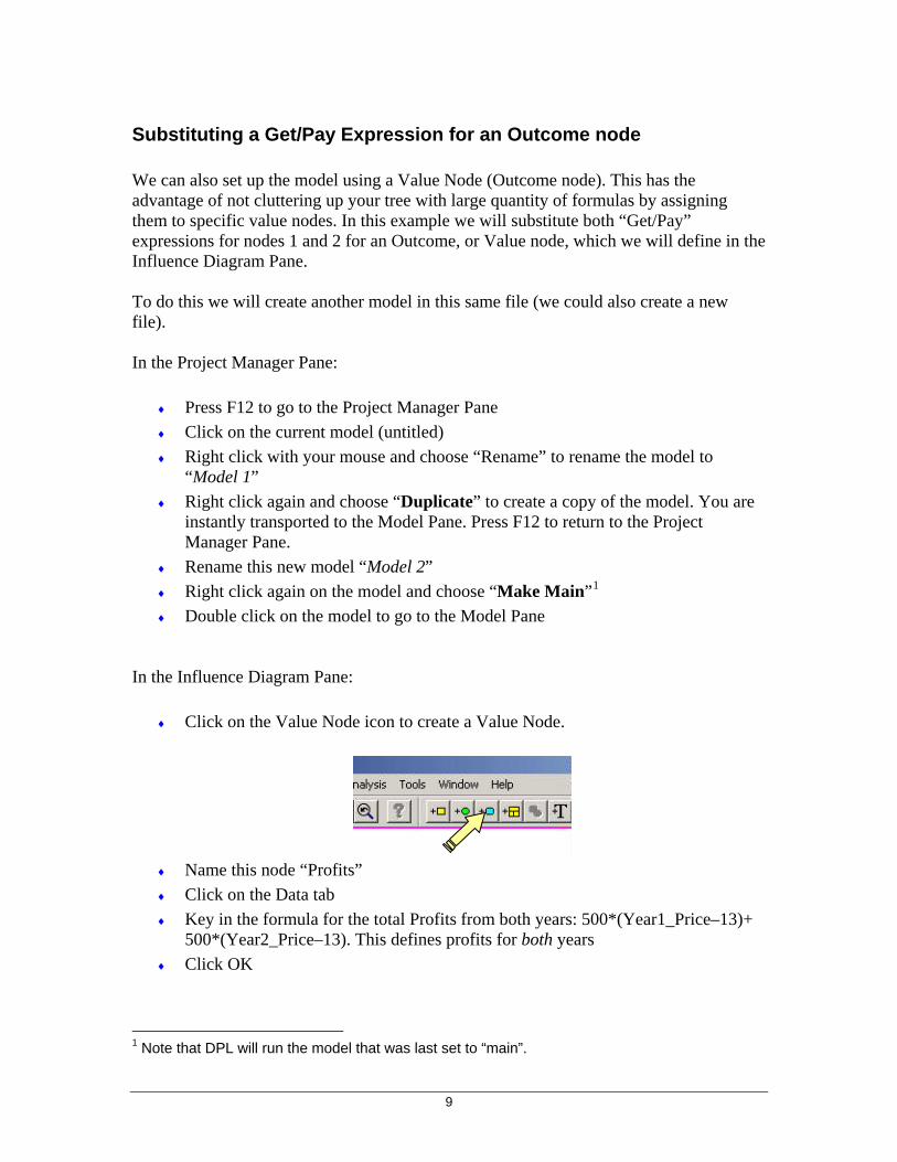
♦ Click on the Value Node icon to create a Value Node.

♦ Name this node “Profits” ♦ Click on the Data tab

Key in the formula for♦ the total Profits from both years: 500*(Year1_Price–13)+ 500*(Year2_Price–13). This defines profits for both years Click OK ♦

1 Note that DPL will run the model that was last set to “main”.

9

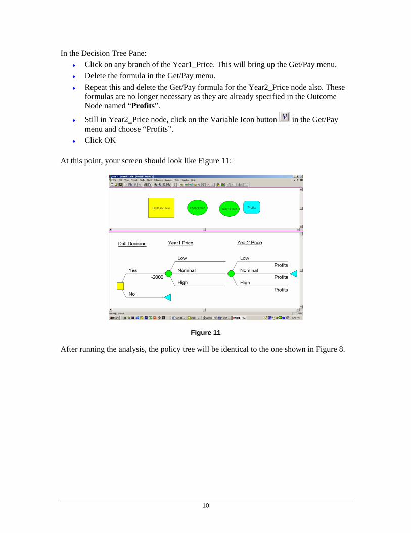
In the Decision Tree Pane: of the Year1_Price. This will bring up the Get/Pay menu.

a for the Year2_Price node also. These

♦ k on the Variable Icon button

♦ Click on any branch ♦ Delete the formula in the Get/Pay menu. ♦ Repeat this and delete the Get/Pay formul

formulas are no longer necessary as they are already specified in the Outcome Node named “Profits”.

Still in Year2_Price node, clic in the Get/Pay

♦

At this point, your screen should look like Figure 11:

menu and choose “Profits”. Click OK

Figure 11

After running the analysis, the policy tre entical to the one shown in Figure 8. e will be id

10

Modeling a Lognormal Distribution with a binomial lattice Rather than inputting all the expected future prices of an asset, we can assume that prices will follow a certain distribution, and have the model compute what these values will be. Let’s assume that a NBI Inc’s current stock price is $100, the volatility is 30% per year, and that stock prices follow a lognormal distribution. We can model these prices with a binomial lattice, where the up state has a value of tu eσ= and d = 1/u. The probability is

given by rte dpu d−

=−

. We will create a 5 year model (t=1), where r = 5%.

Open a new DPL file. In the Influence Diagram Pane:

♦ Click on the Value Node icon to create a Value Node. We will use these for our constants.

♦ Name this “u” ♦ Click on the Data tab ♦ Input the formula for u = exp (0.30) ♦ Click Enter and OK

♦ Click on the Value Node icon to create a Value Node. ♦ Name this “d” ♦ Click on the Data tab ♦ Input the formula for d = 1/u ♦ Click Enter and OK

♦ Click on the Value Node icon to create a Value Node.

Name this “r” ♦

Click on the Da♦

♦ Input the value for r. (0ta tab

.05)

♦ Click on the Value Node icon to create a Value Node.

ata tab )

♦ Click on the Value Node icon to create a Value Node.

ta tab

♦ Click Enter and OK

♦ Name this “t” ♦ Click on the D♦ Input the value for t. (1♦ Click Enter and OK

♦ Name this “p” ♦ Click on the Da

11

♦ Input the formula for p = [exp(r*t)-d]/(u-d)

♦ Click on the Chance Node icon to create a Chance Node.

that we have only two states: “Up” and “Down”

ility utcome

e

Not o need to enter the down probability, as the model assumes it is (1-p) utomatically. We must now create 5 chance nodes that are very similar. The easiest way

Paste”. A new chance node will appear ew chance node to “ Yr2”

ome

Click “Edit / Copy” and then “Edit / Paste”. A new chance node will appear ew chance node to “ Yr3”

ome

t

e the pane to make this the active pane ♦ All 5 Chance Nodes are already in place.

ps up.

pt for the last one (Yr5).

♦ Click Enter and OK

♦ Name this node “Yr1” ♦ Modify the outcomes so♦ Click on the Data tab ♦ Input “p” as the probab♦ Input $100*u for the “Up” o♦ Input $100*d for the “Down” outcom♦ Click OK

e that there is nato do this is to make a copy of this node and then edit in the modifications.2

♦ Click on the “Yr1” node ♦ Click “Edit / Copy” and then “Edit /

Change the name of the n♦

♦ In the Data tab, replace “100*u” with “Yr1*u” for the “Up” outcome ♦ Replace “100*d” with “Yr1*d” for the “Down” outc ♦ Click on the “Yr2” node ♦

♦ Change the name of the n♦ In the Data tab, replace “Yr1*u” with “Yr2*u” for the “Up” outcome ♦ Replace “Yr1*d” with “Yr2*d” for the “Down” outc Repeat for Chance Nodes “Yr4” and “Yr5”.

In he Decision Tree Pane:

♦ Click anywhere insid

♦ Click on any branch of the “Yr1” node. The Get/Pay menu po♦ Delete the formula there and leave it blank♦ Click OK ♦ Repeat for all chance nodes of the tree exce

2 Unfortunately this does not work with Student Version 4.0, only with the Full Version

12

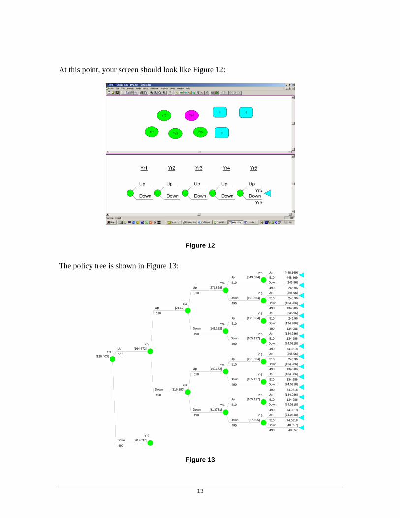
t t A his point, your screen should look like Figure 12:

Figure 12

The policy tree is shown in Figure 13: Up

448.169 .510

[448.169] Yr5 Up

.510

[349.034]

Down

245.96 .490

[245.96]

Up

245.96 .510

[245.96]

Down

134.986 .490

[134.986]

Yr5 Down

.490

[191.554]

Yr4 Up [271.828]

.510

Up

245.96 .510

[245.96]

Down

134.986 .490

[134.986]

Yr5 Up

.510

[191.554]

Up

134.986 .510

[134.986]

Down

74.0818 .490

[74.0818]

Yr5 Down

.490

[105.127]

Yr4 Down

.490

[149.182]

Yr3 Up

.510

[211.7]

Up

245.96 .510

[245.96]

Down

134.986 .490

[134.986]

Yr5 Up

.510

[191.554]

Up

134.986 .510

[134.986]

Down

74.0818 .490

[74.0818]

Yr5 Down

.490

[105.127]

Yr4 Up

.510

[149.182]

Up

134.986 .510

[134.986]

Down

74.0818 .490

[74.0818]

Yr5 Up

.510

[105.127]

Up

74.0818 .510

[74.0818]

Down

40.657 .490

[40.657]

Yr5 Down

.490

[57.695]

Yr4 Down

.490

[81.8731]

Yr3 Down

.490

[116.183]

Yr2 Up

.510

[164.872]

Yr2 Down

.490

[90.4837]

Yr1 [128.403]

Figure 13

13

This tree gives us the distribution of k five years out. This distribution is lognormal. We can use this model to calculate the price of options written on this stock.

uropean Call Option

uropean Call Option on NBI’s stock, with strike price of 80 and 5 years to expiration.

♦ Press F12 to go to the Project Manager Pane lained previously, create a new model named “European

♦ this module the “Main” module

th♦ Click on the Value Node icon to create a Value Node.

rice”

n to create a Decision Node node “Exercise?”

In the Decision Tree Pan e to make this the active pane

d Decision” in the pull down menu.

ance Menu

p the

NBI’s stoc

E

Suppose we want to value a E1 In the Project Manager Pane:

♦ Following the steps expCall”

♦ Double click on the model to go to the Model Pane Make

In e Influence Diagram Pane:

♦ Name this node “Strike P♦ Click on the Data tab ♦ Key in 180 for the strike price ♦ Click OK ♦ Click on the Decision Node ico♦ Name this

e: Click anywhere inside the pan♦

♦ Click on “Node / Ad♦ Choose the only option available which is “Exercise?” ♦ Attach this decision node to the “Yr5” chance node

t♦ Click on the “Exercise?” node. This will bring up the Ins♦ Choose “Asymmetric”

Click on the “Yes” branch of the “Exercise?” node. ♦ This will bring uGet/Pay Menu.

♦ button Using the Variable Icon to input the formula “(Yr5 - Strike_Price)/exp(0.05*5)”.3

3 If exercised in year 5, the payoff of the option will be the Year 5 Price less the Strike Price. This

value must be discounted 5 periods at the riskfree rate to arrive at it’s Present Value. If not exercised, the payoff is zero, which is the automatic assumption of DPL trees whenever no value or formula is provided in the branch.

14

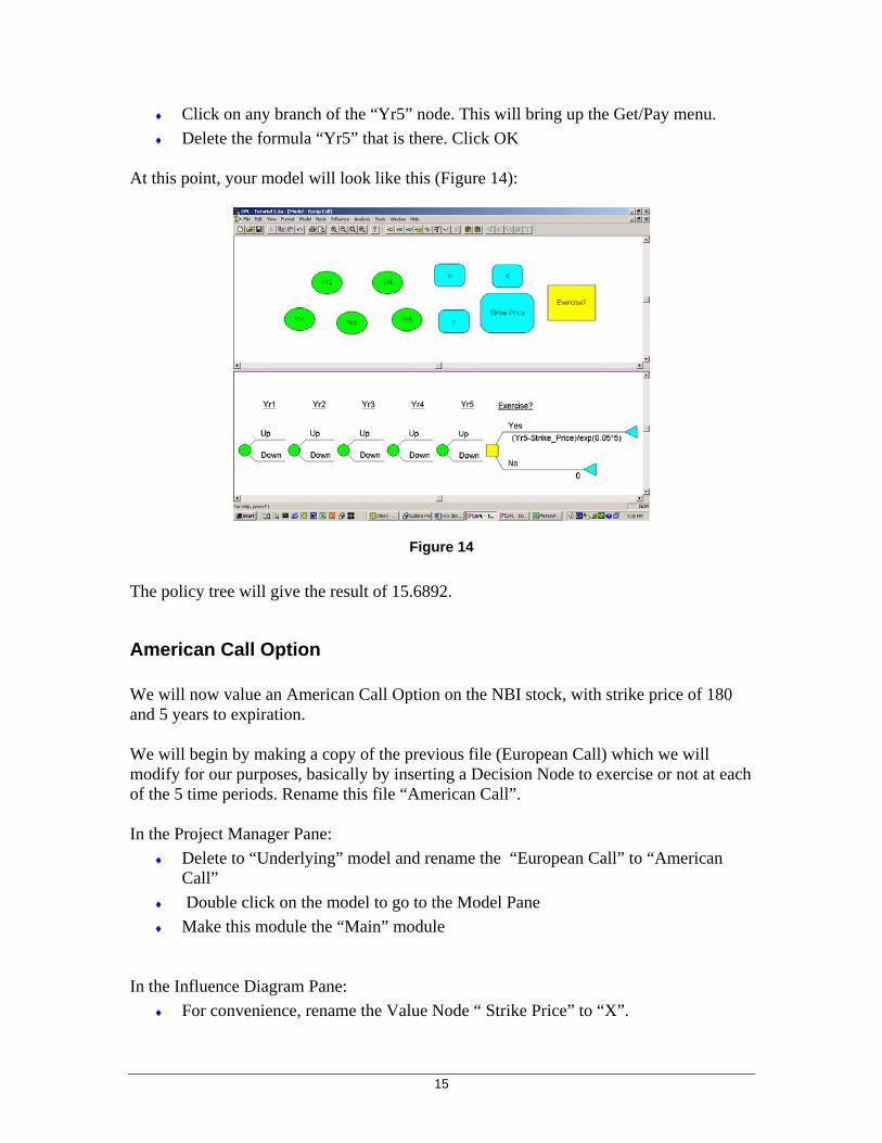
♦ Click on any branch of the “Yr5” node. This will bring up the GeDelete the formula “Yr5” that

t/Pay menu. ♦ is there. Click OK

At this point, your model will look like this (Figure 14):

Figure 14

The policy tree will give the result of 15

can Call Option on the NBI stock, with strike price of 180

sically by inserting a Decision Node to exercise or not at each

ropean Call” to “American

♦

.6892.

American Call Option We will now value an Ameriand 5 years to expiration. We will begin by making a copy of the previous file (European Call) which we will modify for our purposes, baof the 5 time periods. Rename this file “American Call”. In the Project Manager Pane:

♦ Delete to “Underlying” model and rename the “EuCall”

♦ Double click on the model to go to the Model Pane Make this module the “Main” module

In the Influence Diagram Pane:

♦ For convenience, rename the Value Node “ Strike Price” to “X”.

15

♦ Rename the Decision Node “Exercise?” to “ Exercise5?” py/Paste)

♦ Rename each of these new Decision Nodes “Exercise1”, Exercise2”, “Exercise3” and “Exercise4?”

In t 4.

♦

tree. d Decision” in the pull down menu.

♦

his decision node to the “Yr1” chance node e Menu

♦ of the “Exercise1?” node. This will bring up the

r1-X)/exp(0.05*1)”. Click OK. ) branch.

” node and choose “Detach”. This will separate this node

♦ / Add Decision” in the pull down menu.

Click on the “Exercise2” node. This will bring up the Instance Menu

♦

nd attach it to the lower (“No”) branch.

Exercise4”) At

♦ Make four copies of this node (Edit/Co

he Decision Tree Pane:

We will now insert these new nodes at t=1, t=2, t=3 and t=

♦ Click anywhere inside the pane to make this the active pane Right Click on the “Yr2” node and choose “Detach”. This will separate this node from the rest of the

♦ Click on “Node / AdChoose “Exercise1”

♦ Attach t♦ Click on the “Exercise1” node. This will bring up the Instanc♦ Choose “Asymmetric”

Click on the “Yes” branchGet/Pay Menu.

♦ Input the formula “(Y♦ Drag the “Yr2” node and attach it to the lower (“No”

♦ Right Click on the “Yr3

from the rest of the tree. Click on “Node

♦ Choose “Exercise2” ♦ Attach this decision node to the “Yr2” chance node ♦

♦ Choose “Asymmetric” Click on the “Yes” branch of the “Exercise2?” node. This will bring up the Get/Pay Menu.

♦

Drag the “Yr3” node aInput the formula “(Yr2-X)/exp(0.05*2)”. Click OK.

♦

Repeat this procedure for the last two Decision Nodes. (“Exercise3” and “

this point, your model should look somewhat like in Figure 15:

16

Exercise2

Yes (Yr1-X)/exp(0.05*1) Yes

(Yr2-X)/exp(0.05*2)

Yes (Yr3 - X)/exp(0.05*3)

Yes (Yr4-X)/exp(0.05*4)

Yes (Yr5-X)/exp(0.05*5)

No

Up

Down

Exercise5

No

Yr5

Up

Down

Exercise4

No

Yr4

Up

Down

Exercise3

No

Yr3

Up

Down No

Yr2Exercise1

Up

Down

Yr1

Figure 15

The policy tree will give the result of 15.6892. Note that this is the same result as with the European Option. This was expected, because we know that it is never optimal to exercise American Options early.

Linking DPL to a Spreadsheet

L model to account for chance events and decision nodes.

nked to specific spreadsheet cells

♦

In t

♦ y setting up your spreadsheet model. lls.

♦

spreadsheet will function basically as a subroutine of your DPL e spreadsheet (export link to a

f a calculation (import link to a cell

Let’s st rom a spreadsheet. For this we will use the spre

♦

♦ You can create a spreadsheet in Excel and then have DPL automatically build a deterministic model from this spreadsheet by linking DPL to this spreadsheet. Then you can edit your DP

♦ Specific DPL variables can be li♦ Data can be sent both from DPL to the spreadsheet and from the spreadsheet to

DPL. In a sensitivity analysis, for example, DPL will send a parameter to the spreadsheet and request an outcome for that particular scenario, which will then be returned to DPL as an outcome value.

he Spreadsheet: Start b

♦ Only named cells will be linked – you must name all input and output ceSpreadsheet must be set up to define one scenario only – DPL is the one that willbe doing the sensitivity analysis.

♦ Note that themodel, or a black box – DPL will send data to thcell with a constant) and get back the result owith a formula).

art by building a deterministic model fadsheet file ChinaOil.xls.

Open a new blank DPL model window

17

♦

♦ aOil.xls” spreadsheet.

ision Analysis” pull down menu.

. Use the Variable Icon button

Click on “Tools / Create Model from Excel”. Choose the “Chin

♦ Click OK. The Influence Diagram of the model appears. ♦ Click on “Format / Arrange Diagram / Left-to-Right” to rearrange the model on

the screen. (Figure 16) Run the model by clicking on “Analysis♦ / Dec

♦ DPL will ask which variable to calculate to ake,

me as the spreadsheet. This means that there is 0%

choose “NPV”. (Since this is a deterministic model with no decision to mthere is no decision tree.)

♦ In the Risk Profile graph we can see that the expected value is 88 (on the horizontal scale), the saprobability that the NPV will be less than 88, and 100% probability that the NPVwill be greater or equal 88.

ReservesProdRate

DeclineRate

OperatingCost

FixedCostOilPrice

PSCShareDevelCost

NPV

Figure 16

Adding Uncertainty

♦ We can now add uncertainties to this deterministic model by changing Value nodes into Chance nodes.

♦ Let’s begin by inserting an uncer e Oil Price. We do this by changing this Value node into a chance node.

il Price node. Click on “Change Node Type” and choose “Chance” to change this node into a Chance node.

ape e Diagram pane has changed to a circle.

tainty in th

♦ Right click on the O

♦ When the Node Definition window appears, click OK. You will see that the shof this node in the Influenc

♦ Double click on the Oil Price node again. The Data window will appear.

18

♦ The three uncertain outcomes (Low, Nominal, High) have the same original vaof $15. We will now change that to $10, $15 and $2

lue 5 respectively, to cover the

lthough igh as

♦

♦

al

The inf Notice the cha Nodes.

range of possible oil prices for the problem, while maintaining the default probabilities for now.

♦ Let’s assume that there is also uncertainty over the level of the reserves. Athe reserves are estimated to be 90MM Bbl it could be as low as 50 or as h200M.

Right click on the Reserves node. Click on “Change Node Type” and choose “Chance” to change this node into a Chance node.

♦ When the Node Definition window appears, click OK. You will see that the shape of this node in the Influence Diagram pane has changed to a circle.

Double click on the Reserves node again. The Data window will appear.

♦ The three uncertain outcomes (Low, Nominal, High) still have the same originvalue of 90. We will now change that to 50, 90 and $200 respectively and click OK.

luence diagram for the model should look somewhat like Figure 17. nge in shape (and color) of the two nodes we modified from Value to Chance

ProdRate

DeclineRate

Reserves

OperatingCost

NPV

FixedCostOilPrice

PSCShareDevelCost

Figure 17

♦ We will now run our analysis again, by clicking on “Analysis/Decision Analysis” on the pull down menu. We get the Policy Tree shown in Figure 18. We can also see that the Expected NPV of the project has increased from 88 to 175.8 due to range of possible values for the uncertain variables that we input.

19

Low -63.029 .300

[-63.029]

Nominal -42.9486 .400

[-42.9486]

High 14.9338 .300

[14.9338]

Reserves Low .300

[-31.608]

Low 15.1398 .300

[15.1398]

Nominal 87.9444 .400

[87.9444]

High 293.954 .300

[293.954]

Reserves Nominal .400

[127.906]

Low 174.977 .300

[174.977]

Nominal 350.058 .400

[350.058]

High 848.888 .300

[848.888]

Reserves High .300

[447.183]

OilPrice [175.835]

Figure 18

Determining the relevant Uncertainties Attempts to model all uncertainties in a project are time consuming and unnecessary, as not all uncertainties have a relevant effect on the project’s NPV. DPL can help you determine which uncertainties are relevant by means of a Tornado graph.

♦ Click on “Analysis/Expected Value Tornado Diagram”

♦ In “Value for Sensitivity” choose “Production Rate” and click OK

♦ Enter the low and high values of 0.08 and 0.12.

♦ Click on “Next Value”, choose “Operating Cost” and enter 6 and 11 for the low and high values.

♦ Click on “Next Value”, choose “Development Cost” and enter 60 and 100 for the low and high values.

♦ Click on “Next Value”, choose “PSC Share” and enter 0.22 and 0.27 for the low and high values.

♦ Click on “Run Now”. The Tornado Diagram of Figure 19 indicates that Operating Cost and Production Rate uncertainties have a much larger impact on the profitability of the project than Development Costs and PSC Share. This means you definitely want to model these first two uncertainties, but may pass on the other less important ones.

20

OperatingCost

ProdRate

DevelCost

PSCShare

80 100 120 140 160 180 200 220

Figure 19

Using Utilities DPL allows for a very simple means of using a utility function to model risk attitudes. The Strenlar case is a good example of how the risk attitude as modeled by an utility function can influence the decision making process.

♦ Open the Strenlar1.da file and run the analysis. We get the Policy Tree shown in Figure 20 that indicates that the optimal alternative for Mr. X is the riskier of developing the product on his own.

Lawsuit Develop

-200 [3632]

Technology Salary [2017.95]

Technology Cash_Offer [1004.88]

Strenlar_Decision [3632]

Figure 20

♦ Now suppose Mr. X is risk averse. A good model for this behavior is an exponential utility function, which can be totally defined by Mr. X risk tolerance, which we will assume to be 500.

♦ On the pull down menu, go to “Model/Risk Tolerance” and enter the value of 500.

♦ Run the analysis again. We now get a Policy Tree (Figure 21) that clearly indicates that given that Mr. X is somewhat risk averse, the optimal course of action in this case is to go with the less risky alternative of accepting a salary in the firm plus royalties.

21

Lawsuit Develop

-200 [111.508]

Technology Salary [1113.54]

Technology Cash_Offer [926.162]

Strenlar_Decision [1113.54]

Figure 21

♦ Now suppose Mr. X risk tolerance is lower, maybe 200. On the pull down menu, go to “Model/Risk Tolerance” and enter the value of 200 and run the analysis again.

♦ The new Policy Tree (Figure 22) show that such a low risk tolerance (indicating a very risk averse attitude) Mr. X should go for the alternative with the lowest risk of all, mainly the upfront cash offer.

Lawsuit Develop

-200 [-84.7736]

Technology Salary [659.817]

Technology Cash_Offer [790.407]

Strenlar_Decision [790.407]

Figure 22

Note: Values inserted in the Node Data are not automatically added to the tree. They must be specifically invoked from formulas or a “Get/Pay” expression. Values inserted as “Get/Pay” are automatically included into the tree calculations.

Linking to spreadsheet ♦ Suppose you linked your DPL model to a spreadsheet and now you want to add an

additional node link. If you just re-link it will delete your whole DPL file ♦ What you want to do is: ♦ Tools/Add linked nodes/From Excel

22

♦ When the window appears, click on the Browse button to re-choose the Excel file to link

♦ Click “Select” ♦ A new window now appears showing any Excel name that has not yet been linked ♦ Choose the one you want and close all

23