A BRANCH-AND-PRICE APPROACH FOR A MULTI-TRIP VEHICLE

September 24-28, 2012Rio de Janeiro, Brazil

A BRANCH-AND-PRICE APPROACH FOR A MULTI-TRIP VEHICLE ROUTING

PROBLEM WITH TIME WINDOWS AND DRIVER WORK HOURS

Michel Povlovitsch Seixas

Department of Naval and Ocean Engineering, University of São Paulo.

Av. Prof. Mello Moraes, 2231, 05508-030. São Paulo, SP, Brazil.

[email protected]

André Bergsten Mendes

Department of Naval and Ocean Engineering, University of São Paulo.

Av. Prof. Mello Moraes, 2231, 05508-030. São Paulo, SP, Brazil.

[email protected]

ABSTRACT

This study considers a vehicle routing problem with time windows, accessibility restrictions on

customers and a fleet that is heterogeneous with regard to capacity and average speed. A vehicle

can perform multiple routes per day, all starting and ending at a single depot, and it is assigned to

a single driver, whose total work hours are limited. A column generation algorithm embedded in

a branch-and-bound framework is proposed. The column generation pricing subproblem required

a specific elementary shortest path problem with resource constraints algorithm to deal with the

possibility for each vehicle to perform multiple routes per day and to deal with the need to

determine the workday beginning instant of time within the planning horizon. To make the

algorithm efficient, a constructive heuristic and a metaheuristic based on tabu search were also

developed.

KEYWORDS: Routing, Tabu Search, Column Generation, Dynamic Programming, Branch-and-

price.

L & T - Logistics and Transport

PM - Mathematical Programming

3469


1. Introduction

The transportation activity is a very important area in the logistic context and absorbs, on

average, a higher percentage of the total costs than the other logistic activities (Ballou, 2001).

A variant of the vehicle routing problem with time windows (VRPTW) is considered herein,

highlighting that each vehicle is assigned to a single driver who can travel several routes during a

workday and be within the limit of his/her working hours. This feature requires identification of

the optimal point in time to start each route. Some customers have accessibility restrictions,

thereby requiring specific vehicles. Concerning the objective function, the purpose is to minimize

the total routing cost, which depends both on the distance travelled and on the vehicle used.

Great advancements have been obtained for different VRPTW variants, such as that by Solomon

and Desrosiers (1988). Desrochers et al. (1992) propose the use of the column generation

technique to solve the linear relaxation of the VRPTW set partitioning formulation; the same

approach employed in the present study.

Obtaining solutions to the vehicle routing problem with multiple routes, but without time

windows, has been approached by means of heuristics such as by Taillard et al. (1996), Brandão

and Mercer (1998) and Petch and Salhi (2003, 2007). In the study by Taillard et al. (1996),

different routes generated by tabu search are combined to produce workdays through the

resolution of a bin-packing problem. In this work, the tabu search developed acts on a space with

multiple routes without the need to combine them to form workdays. This approach, albeit more

costly for seeking neighbour solutions within a larger space, eliminates the computational cost of

analyzing the feasibility of combining different routes and of finding a good combination.

Azi et al. (2010) proposed an exact algorithm to solve the VRPTW with multiple routes based on

a branch-and-price algorithm. The pricing subproblem consisted in finding a sequence of routes,

i.e. a workday, on the routes generated at a preprocessing stage. Differently, in the problem

studied, the subproblem finds a sequence of customers in order to generate a workday.

Concerning the treatment usually given to a workday, it is considered that a number of working

hours cannot be exceeded in each route, forcing the last customer to be served within a maximum

time interval occurring after the beginning of the route serving it (Azi et al., 2010). However, in

this study, a similar control is necessary but applied to multiple routes forming a workday.

It is also worth stressing that the classical dynamic programming algorithms developed to solve

the shortest path problem with resource constraints, such as in Dejax et al. (2004), do not make

considerations on the determination of the beginning of each vehicle path in relation to the

planning horizon. In the present study, the beginning instant of the workday is a decision to be

made together with the determination of the sequence of customers to be visited.

This characteristic, together with the possibility of the vehicle being able to conduct multiple

routes per day, was treated by a specific algorithm to solve the subproblem in the ambit of

column generation – this being the major contribution of this work, besides a complete

framework to solve the problem which contains also: a constructive heuristic, a very effective

tabu search and a branch-and-price procedure.

It should be stressed that the vehicle routing problem considered in this study generalizes the

VRPTW and is therefore NP-hard (Lenstra and Rinnooy, 1981).

The paper is organized as follows: Section 2 provides a brief description of the problem studied

and of the objective function to be optimized; Section 3 presents a mathematical formulation;

Section 4 describes procedures and algorithms; Section 5 presents parameter settings, instances

and the results obtained. Conclusions are given in section 6.

2. Problem Description

The vehicle routing problem studied consists of determining the workday of each vehicle of the

fleet to minimize the total cost of the distribution operation from a single depot. A vehicle

workday is defined as a sequence of customers to be visited; for this purpose, the vehicle may

return to the distribution center to be reloaded and then start a new delivery route. A workday,

therefore, consists of a feasible sequence of routes throughout the day. For convenience purposes,

the maximum number of routes in a workday is predetermined. Vehicles that are not eventually

used run the fictitious route in which a vehicle leaves the distribution center and returns to it

3470


without visiting any customer, at no cost. Demand is previously known before the day starts and

every customer must be served only once. Besides, each customer has a specific service time and

a strict time window that must be respected. If the vehicle reaches a customer before the opening

of its time window, it must wait until the time window opens to begin the service. If the vehicle

arrives after the end of the time window, the service is not provided. Some customers can only be

visited by specific vehicles due to accessibility restrictions at the delivery location. The fleet is

heterogeneous in capacity and in average displacement speed. The cost of using a vehicle is

variable, only depending on the total distance traveled. The total number of hours worked by the

driver in a workday cannot exceed a specified maximum limit. The vehicle loading time at the

distribution center before the beginning of each route and possible waiting times at customers’

locations until the opening of their time windows are considered in the calculation of the worked

hours, along with the travelling time between customers and the service time at each of them. The

traveling times depend on both the distance traveled and the average speed of the vehicle used.

3. Mathematical Formulation

Digraph ( ) is given where is the set of customers; and are

fictitious origin and destination vertices, respectively, both corresponding to the depot; is the

set of arcs joining two distinct vertices of ; and any feasible route corresponds to a path from

to on . Let represent the maximum number of routes driven during a vehicle workday.

To represent a workday with routes, digraph is sequentially replicated times, forming

digraph , in which a path from (origin of route 1) to (destination of route ) represents

a vehicle workday with the routes (see figure 1). Vehicles not used in route during the

workday travel the fictitious arc ( ) at zero cost.

Figure 1: example of a digraph regarding one vehicle and its workday.

Computationally, only a reduced digraph of a single route is stored and used so that memory

consumption is not significantly increased. An instance is defined by the following data:

- Directed graph ({ } { } ).

- Set of heterogeneous vehicles .

- – set of customers to be served by specific authorized vehicles: .

- Each customer has a group of authorized vehicles : .

- – maximum capacity of vehicle , in units.

- [ ] – time window of customer . For the vertices { } representing the

distribution center (depot), the time windows correspond to the planning horizon, i.e.,

[

] [

] [ ] [ ].

- – customer demand, in units.

- – service time at customer , which is identical for all vehicles. At the distribution

center, this corresponds to the average loading time .

- – cost of traveling the arc ( ) with vehicle in route .

- – travel time of arc ( ) with vehicle .

- – maximum duration of a vehicle workday.

3471


- – maximum number of routes allowed per day for the vehicles. This is an upper bound

that is large enough to encompass all possible trips according to past daily routing

operation experiences.

- is a sufficiently large number:

{ } ( ) .

The mathematical model developed, IP, has two decision variables: – binary variable that is

equal to 1 if arc ( ) is traveled by vehicle in route and equal to 0 otherwise, – variable

that defines the instant of time at which vehicle will serve customer in route .

(IP) ∑ ∑ ∑ ∑

{ } { }

s.t.

∑ ∑ ∑

{ } (1)

∑ ∑

{ } (2)

∑

{ } (3)

∑

{ } (4)

∑

{ } ∑

{ } (5)

{ } (6)

(

) ( ) {( )} (7)

( )

( ) ( ) (8)

∑ [

(∑

{ } )] (9)

(10)

{ } ( ) (11)

{ } (12)

Constraint (1) imposes that each customer must be visited only once by a vehicle in a route .

According to constraint (2), unauthorized vehicles are kept from visiting customers that have

accessibility restriction. In (3), it is imposed that every vehicle has to leave from each route

origin. Analogously, constraint (4) imposes that every vehicle must reach each route

destination. Constraint (5) ensures the flow conservation in a customer. Constraint (6) imposes

that time windows must be respected. The group of constraints (7) and (8) establishes the

relationship between the vehicle departure time from a customer and its immediate successor.

Constraint (9) states that a vehicle can only be loaded up to its capacity. Constraint (10)

guarantees that the workday duration of a vehicle does not exceed its limit . The group of

constraints (11) and (12) defines the solution space of the decision variables.

4. Resolution Algorithm

To solve the problem formulated in section 3, it is proposed a branch-and-price procedure based

on arc flow variable cuts resulting from branching decisions of the type and

. A

constructive heuristic and a metaheuristic based on tabu search were also developed. It is

described: Constructive Heuristic, Tabu Search, Extensive Formulation and Column Generation,

Pricing Subproblem and Branch-and-Price.

4.1. Constructive Heuristic

In summary, the developed procedure inserts customers into vehicle workdays and builds an

initial solution after inserting all of them according to the pseudocode Constructive_Heuristic.

Constructive_Heuristic Algorithm – procedure to find a feasible solution.

1 find customers’ geometric center

2 divide customers in 4 quadrants with their geometric center as a reference

3 sort each quadrant list of customers in increasing order of time window opening

4 //Travel quadrants in anti-clockwise sequence//

5 for each quadrant customer list do

6 for every customer with a list of authorized vehicles do

3472


7 find the smallest insertion cost position among authorized vehicle

workdays

8 if a position was found then

9 insert customer and remove it from the quadrant list

10 sort vehicles in decreasing order of cargo capacity

11 sort vehicles in increasing order of cost (variable or fixed) with a stable sorting algorithm

12 for each vehicle in the sorted list of vehicles do

13 //Travel quadrants in anti-clockwise sequence//

14 for each quadrant customer list do

15 for each customer do

16 find smallest insertion cost position in current vehicle workday

17 if a position was found then

18 insert customer and remove it from quadrant list

19 if there are unserved customers then

20 if tabu search was never called then

21 call tabu search to improve current solution

22 go to line 5 to insert unserved customers

23 else

24 call a commercial software to find a feasible solution (60s of time limit)

It should be stressed that the customer insertion procedure above does not consider cuts in arc

flow variables of the type . Hence, a preprocessing is conducted to generate workdays

that consider all the cuts. For this, a solution with as few customers as possible is found by

solving the elementary minimum cost path problem of each vehicle, where the cost of traveling

an arc is equal to its distance. Each vehicle is treated sequentially and the customers visited in the

solution of a vehicle are prevented from being visited by the other vehicles not yet treated. No

feasible solution exists in case it is not possible to find a solution to this problem for any of the

vehicles. Only after obtaining workdays which do not violate any cut, the procedure previously

described will be executed to insert customers that have not been allocated yet.

4.2. Tabu Search

Tabu search is a metaheuristic with wide application in vehicle routing problems (see Bräsy and

Gendreau, 2005), which combines intensification and diversification strategies, using short and

long-term memories. For the problem studied, the single insertion move as well as a customer

repositioning move within a vehicle workday, were used as moves to find neighbour solutions.

Also, rather than employing long-term memory to help with the diversification process, a

predefined number of random moves is performed. The aspiration criterion adopted is the

acceptance of a tabu solution when it globally improves the objective function and its cost is

lower than the best non tabu solution.

The major parameters for calibrating the tabu search are: size of the short-term memory; number

of iterations without minimum local solution improvement that triggers diversification; number

of random moves to diversify a solution and maximum number of diversifications.

In each iteration, all possible moves are verified. If there is a move which has removed the

customer from the destination vehicle workday in the short-term memory, then the move under

analysis is tabu. Also in the present implementation, when a move fails to improve the minimum

local solution, it is verified whether the maximum number of iterations without minimum local

solution improvement was reached. In this case, a diversification will be executed.

Diversification is carried out by randomly choosing customer reallocation moves between

vehicles. Tabu search ends when the maximum number of diversifications is reached.

4.3. Extensive Formulation and Column Generation

It is possible to provide an alternative formulation to the routing problem, after observing that IP

has primal block diagonal structure. This structure is composed by linking constraints (1) and

independent constraint blocks from (2) to (12) of each vehicle , corresponding to workdays. Let

3473


be the set of all feasible workdays of vehicle . The mathematical formulation of the

problem, denoted Master Problem (MP), is the following:

(MP) ∑ ∑

s.t.

∑ ∑

(13)

∑

(14)

{ } (15)

where is a binary decision variable equal to 1 if and only if workday is choosen for vehicle

and 0 otherwise; ∑ ∑ ∑

{ } { } for is the cost of

workday of vehicle ; ∑ ∑

{ }

for is the number of

times customer is visited by vehicle on workday ; { } for

( ) is equal to 1 if on workday , vehicle in route travels the arc ( );

, otherwise. Constraints (13) impose that each customer must be served only once.

Constraints (14) impose that exactly one duty is selected for each vehicle. Constraints (15) ensure

that the solution is integer. We remark that MP has an exponential number of variables.

Therefore, we resort to column generation (Desrosiers and Lübbecke, 2005) to solve the linear

relaxation of the master problem (LMP). In LMP, the set partitioning constraints (13) are

replaced with set covering constraints: ∑ ∑

for . Set covering

constraints are preferable with respect to set partitioning constraints as the associated dual

variables are restricted to assume non-negative values.

To solve LMP, we apply column generation. Therefore, we consider a subset of workdays for

each vehicle obtaining a restricted master problem (LRMP) so that a feasible solution to LMP

exists. We solve the LMP and consider dual variables and associated with constraints (13)

and (14), respectively. We solve a pricing subproblem for every vehicle and iterate the

algorithm until no column with negative reduced cost exists for every vehicle. The pricing

subproblem consists in finding a workday that potentially contributes to reducing the objective

function of LRMP, that is, a workday whose reduced cost of the new variable is negative. The

pricing subproblem, SP, has the objective function ∑ ∑ ∑ ( ) { } { }

, where

for , subject to constraints (2)…(12) of vehicle .

4.3.1. Initialization

The LRMP of each tree node is initialized with a good initial solution provided by the heuristic at

low computational cost. In most cases, it was observed that the number of columns generated to

the LRMP optimality is reduced significantly with a good initial solution.

4.3.2. Lower Bounding and Anticipated Finalization

In some cases, it is possible to interrupt the column generation scheme before obtaining the

optimal solution with the calculation of a lower bound, , according to expression:

∑ | | where is the optimal solution of the vehicle subproblem (Desrosiers

and Lübbecke, 2005). If the value is higher than the incumbent solution objective value, the

generation of new columns is stopped because it is a case of pruning by bound.

4.4. Pricing Subproblem

The pricing subproblem SP can be cast to the computation of an elementary minimum cost path

considering resources constraints (ESPPRC) in digraph , in which the costs in the arcs are

modified according to the shadow prices of constraints (13) of LRMP. A common and widely

employed technique for solving this problem is dynamic programming, as successfully used by

Desrosiers et al. (1995) and by Dejax et al. (2004).

4.4.1. Dynamic Programming Algorithm

The algorithm developed herein was based on the bounded bidirectional dynamic programming

algorithm proposed by Righini and Salani (2006, 2008) which, in turn, is based on the algorithm

3474


developed by Desrochers and Soumis (1988) to solve the resource constrained shortest path

problem, RCSPP. In the present study, the vector of resources is composed of the following

components: (consumed fraction of vehicle capacity), (service start time in a forward label or

departure time in a backward label), (time consumed of the working hours), (idle time

reducing capacity), (number of cuts traveled), (visit vector) and

(number of vertices served along the path). The label also has component that indicates the

route to which the label belongs and the total cost .

When a label ( ) associated to vertex is extended to vertex generating label ( ) the

consumption of each resource is updated according to the rules presented in the next sections;

except for , , and whose rules are the same as those described by Righini and Salani (2008)

and, therefore, are not presented. It is worth emphasizing that the extension from to is only

feasible if the vehicle is authorized to serve customer .

4.4.2. Workload Resource

The calculation of for forward labels is initially defined as { ( )

( )} and for backward labels as { {[ ( )] }} .

However, when the vehicle reaches before in a forward extension or, when the vehicle

departs from after ( ) in a backward extension; idle time is generated. To ensure future

viability, it is necessary to eliminate the maximum idle time as possible. For this, firstly it is

computed the idle time generated: ( ) in a forward extension and in a

backward extension [ ( )] ( ). Then, it is calculated the capacity

to eliminate idle time, : { | ( ) ( )} for forward direction

and { | [ ( )] ( )} for backward direction.

For forward direction, in case and then and

( ). In the other case, when and , then

( ) and ( ) . For backward direction, in case and

then and ( ). In the other case, when

and , then ( ) and ( ).

The forward or backward label created is only feasible if: .

4.4.3. Idle Time Reducing Capacity Resource

The workload resource is not enough to fully identify a label and requires the use of a new

resource capable of identifying the capacity to reduce idle time, , which is updated according to

the procedure described in section 4.4.2 when idle time is generated. If idle time is not generated

and the time window of is not violated then { ( )} for forward labels and

{ [ ( )] } for backward labels. Since , there is no need to

verify whether the extension feasibility is lost in relation to this resource.

4.4.4. Multiple Routes

At first, an initial forward label is added to origin and an initial backward label to

destination . Forward and backward extension procedures are executed until the

list of pending vertices is empty. At this moment, all the forward and dominant labels in are

extended to according to: , , , , ,

, [ ] {

[ ] ; and all backward and dominant labels of are extended to

as follows: , , , , [ ] {

[ ] , if the backward label

does not visit any customer in route then , ; otherwise, , . The label extension process is repeated until in the forward labels and in the

backward labels.

4.4.5. Lexicographic Ordering of Labels

3475


The dominant labels are kept organized in increasing lexicographic order. Label is considered

lexicographically smaller than label if or if .

4.4.6. Bounding on Resource

Based on the strategy adopted by Righini and Salani (2008) to prevent the proliferation of labels

in both directions, a critical resource is selected such that labels consuming over 50% of this

resource are eliminated from each of the two directions. In the problem studied, the critical

resource used is time; hence, a label is discarded when ( ) during an

extension.

4.4.7. Treatment of Arc Flow Variable Cuts

Cuts are easily treated in a preprocessing that eliminates all the arcs related to these cuts.

Cuts are treated by an increasing and unlimited resource ( ) which is initially set

to 0. Whenever a cut is traveled, the resource is incremented. The visit vector ensures

that a cut cannot be counted more than once. The number of cuts of the optimal solution is

always the largest possible due to the use of in the dominance rule.

4.4.8. Dominance Rule

According to the dominance rule used, a label dominates a label if all the expressions

below are true: ; ; ; ; ; ;

; ; and [ ] [ ], { { }}.

4.4.9. Heuristic Labeling Algorithm

Aiming at increasing the convergence speed of the column generation technique, columns are

added by a heuristic labeling algorithm until no new column with negative reduced cost is found,

when the subproblem then starts to be solved to optimality by the exact labeling algorithm

(Ceselli et al., 2009). In the present study, the heuristic labeling algorithm uses a relaxed

dominance rule that does not have the visit vector, , the capacity to reduce idle time, , and

component ( ).

4.4.10. Feasibility Tests and Search for Optimal Solution

The optimal solution is determined after all the feasible combinations between a forward label

and a backward label are verified. For this, there are 7 tests that are applied to ensure that the

combination of two labels, forward in and backward in , is feasible:

1) ;

2) Cut does not exist;

3) The value of added to , plus 1 if cut exists, must be equal to

the total number of mandatory cuts existing in the subproblem of vehicle ;

4) [ ] [ ] 5) , i. e., total capacity is less than or equal to 100% of ;

6) ;

7) After calculating [ ( )] ( ), must be true.

If ( ) then [( ) ] must be true.

Else

Let

If ( ) then [( ) ] must be true.

Else, [( ) ] must be true.

Cost of the combination between label and label is calculated as: .

4.5. Branch-and-Price

The Column Generation algorithm previously described is executed in each tree node under the

branch-and-bound framework. In the next sections, the search strategy, initial upper bound and

branching strategy used are described.

3476


4.5.1. Search Strategies

Three search strategies were implemented: Depth First, Best-Node First and Mixed (Depth First

followed by Best-Node First). The search for the best bound (Best-Node First) strategy was

always used because it had performed better than the others.

4.5.2. Initial Upper Bound

Constructive heuristic and tabu search were used in the root node aiming at starting the branching

with a good upper bound.

4.5.3. Branching Strategy

The branching strategy used for searching the optimal solution was to branch on arc flow

variables, .

5. Computational Results

Solomon’s benchmark vehicle routing problem instances R1 and R2 were adapted to the context

of the problem studied. In the available fleet there are 10 vehicles: 4 trucks, 4 LCVs and 2 vans.

The capacities of a truck, of a LCV and of a van are 200, 120 and 40, respectively. The maximum

workday duration for any driver is ⌊

( )⌋. The cost per unit of distance run by a

truck is 1, by a LCV is 0.75 and by a van is 0.5. The average speeds of a truck, of a LCV and of a

van are 1, 1.333 and 1.666, respectively. In every instance, customer 2 can only be served by a

specific truck and customer 3 can only be served by another specific truck. The depot loading

time is . The tabu search executed at the root node is defined by the parameters as

follows: short-term memory size = 25; number of iterations without improvement that triggers

diversification = 100; number of diversifications = 1000; number of random moves to diversify =

60. In the other nodes, the number of diversifications is reduced to 20.

The results for R1 and R2 instances with the first 20 customers are presented in Tables 1 and 2.

Table 1 – results obtained for R1 instances with the first 20 customers. Instance Route

qty.

Heuristic

cost ($)

Heuristic

time (s)

Root node

cost ($)

Root node

time (s)

Optimal

cost ($)

Total time

(s)

Tree size

(node)

Heuristic

error (%)

R101_20 1 380.309 26.930 380.309 0.284 380.309 27.980 1 0.000 R102_20 1 333.527 35.212 333.527 0.347 333.527 36.240 1 0.000

R103_20 1 312.059 44.621 309.885 0.151 312.059 55.692 27 0.000

R104_20 1 301.855 46.026 294.910 0.464 301.855 840.090 1645 0.000 R105_20 1 340.968 32.992 336.804 0.346 340.968 49.102 81 0.000

R106_20 1 312.598 40.005 312.598 0.457 312.598 41.032 1 0.000

R107_20 1 301.855 48.163 299.842 0.505 301.855 82.432 95 0.000 R108_20 1 301.855 49.514 291.618 0.609 301.855 5735.928 9721 0.000

R109_20 1 309.363 38.908 309.363 3.844 309.363 43.803 1 0.000

R110_20 1 299.211 44.787 297.582 0.529 299.211 63.893 29 0.000 R111_20 1 301.855 51.353 300.419 0.566 301.855 84.417 79 0.000

R112_20 1 297.551 50.449 288.519 0.906 297.551 1752.706 3059 0.000

316.084 42.413 0.751 316.084 734.443 1228 0.000

R101_20 2 380.309 51.607 380.309 0.116 380.309 52.627 1 0.000 R102_20 2 331.018 63.758 330.302 0.179 331.018 74.841 21 0.000

R103_20 2 312.059 78.672 309.855 0.289 312.059 134.955 83 0.000

R104_20 2 300.239 77.568 294.363 0.692 300.239 7917.193 7063 0.000 R105_20 2 340.968 64.402 336.273 0.525 340.968 383.644 1175 0.000

R106_20 2 312.598 70.791 312.510 0.671 312.598 96.857 43 0.000

R107_20 2 301.855 82.422 299.842 0.786 301.855 413.574 487 0.000 R108_20 2 300.239 82.463 291.473 0.925 *298.769 * *81648 0.490

R109_20 2 309.363 69.936 308.963 0.662 309.363 102.073 81 0.000 R110_20 2 299.211 79.388 297.582 0.744 299.211 165.516 89 0.000

R111_20 2 301.855 84.158 298.823 0.630 301.855 625.568 829 0.000

R112_20 2 297.551 85.447 288.519 0.908 297.551 101377.395 55423 0.000

315.605 74.218 0.594 0.041

R101_20 3 380.309 89.951 380.309 0.086 380.309 90.975 1 0.000

R102_20 3 331.018 101.357 330.302 0.702 331.018 122.412 23 0.000

R103_20 3 312.059 126.402 309.885 0.453 312.059 306.011 173 0.000

R104_20 3 300.239 125.063 294.363 1.068 300.239 56773.249 30117 0.000

R105_20 3 340.968 105.662 336.273 0.704 340.968 3038.838 3791 0.000

R106_20 3 312.598 115.196 312.510 0.811 312.598 201.693 121 0.000 R107_20 3 301.855 125.224 299.842 1.036 301.855 3121.445 2639 0.000

R108_20 3 300.239 127.446 291.473 1.452 *296.426 * *91521 1.270

3477


R109_20 3 309.363 111.132 308.963 0.850 309.363 196.550 159 0.000 R110_20 3 299.211 131.971 297.582 0.888 299.211 527.368 275 0.000

R111_20 3 301.855 129.995 298.823 0.950 301.855 2455.952 2447 0.000

R112_20 3 297.551 135.617 288.519 1.687 *295.137 * *86229 0.811

315.605 118.751 0.891 0.173

Value of cells marked with * were not computed due to excessive computing time (greater than 3

days). The corresponding Optimal Cost column is filled with the best lower bound found.


qty.

Heuristic

cost ($)

Heuristic

time (s)

Root node

cost ($)

Root node

time (s)

Optimal

cost ($)

Total time

(s)

Tree size

(node)

Heuristic

error (%)

R201_20 1 321.624 41.136 318.572 0.485 321.624 50.233 33 0.000

R202_20 1 294.230 50.258 287.643 0.791 294.230 93.464 159 0.000 R203_20 1 285.318 57.642 281.365 43.712 285.318 1309.014 113 0.000

R204_20 1 269.632 61.106 264.018 2581.031 269.632 74386.618 139 0.000

R205_20 1 275.590 48.469 273.657 0.577 275.590 58.671 27 0.000 R206_20 1 272.054 60.613 269.999 1.114 272.054 76.701 11 0.000

R207_20 1 272.054 61.823 268.901 56.613 272.054 2616.103 65 0.000

R208_20 1 260.517 65.273 260.517 7644.772 260.517 7710.172 1 0.000 R209_20 1 272.699 57.158 267.426 1.050 272.699 152.635 143 0.000

R210_20 1 285.208 58.032 281.777 1.647 285.208 196.725 79 0.000

R211_20 1 264.974 68.360 263.208 50.218 264.974 793.068 35 0.000

279.445 57.261 943.819 7949.400 73 0.000

R201_20 2 316.940 71.637 313.862 0.734 316.940 107.803 141 0.000

R202_20 2 282.141 90.258 282.141 2.639 282.141 93.286 1 0.000

R203_20 2 278.189 93.647 277.389 806.007 278.189 8522.482 45 0.000 R204_20 2 269.632 99.329 264.018 11446.750 *264.018 * * 2.082

R205_20 2 275.590 82.836 273.657 0.998 275.590 177.311 155 0.000

R206_20 2 272.054 99.500 269.999 7.168 272.054 266.836 37 0.000 R207_20 2 272.054 104.216 268.901 367.263 272.054 124441.694 485 0.000

R208_20 2 260.517 104.118 260.517 19984.943 260.517 20089.802 1 0.000

R209_20 2 272.699 92.700 267.426 1.844 272.699 1326.603 685 0.000

R210_20 2 278.189 97.852 277.874 2.363 278.189 349.628 45 0.000

R211_20 2 264.974 104.130 263.208 103.350 264.974 6406.696 131 0.000

276.634 94.566 2974.914 0.189

R201_20 3 316.940 112.587 313.303 0.738 316.940 1167.372 2889 0.000 R202_20 3 282.141 130.237 282.141 1.699 282.141 132.267 1 0.000

R203_20 3 279.936 140.825 277.389 729.757 278.189 66084.758 241 0.000

R204_20 3 269.632 148.555 264.018 30230.548 *264.018 * * 2.082 R205_20 3 275.590 130.056 273.657 1.531 275.590 520.328 439 0.000

R206_20 3 272.054 146.864 269.999 8.960 272.054 3144.527 455 0.000

R207_20 3 272.054 150.425 268.901 402.199 272.054 253236.878 909 0.000 R208_20 3 260.517 149.460 260.517 129852.202 260.517 130001.852 1 0.000

R209_20 3 272.699 134.581 267.426 3.276 272.699 5460.745 1671 0.000

R210_20 3 278.189 139.620 277.874 32.168 278.189 1910.925 153 0.000 R211_20 3 264.974 149.684 263.208 298.990 264.974 30567.315 379 0.000

276.793 139.354 14687.461 0.189

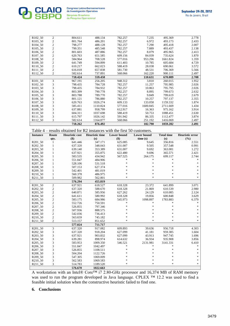
With the same criterion previously used, instances with 50 customers were created. In these

instances, 5 trucks and 5 LCVs were added. As the computational cost becomes high, the 50-

customer instances were solved with the column generation lower bound of the root node as the

problem lower bound. The heuristic parameters were not changed. The final results obtained for

50-customer instances are presented in Tables 3 and 4.


qty.

Heuristic cost

($)

Heuristic time

(s)

Lower bound

($)

Lower bound

time (s)

Total time

(s)

Heuristic error

(%)

R101_50 1 959.872 170.168 948.312 1.861 172.029 1.204

R102_50 1 796.194 286.851 782.257 4.187 291.038 1.750 R103_50 1 799.695 285.119 782.257 3.806 288.925 2.181

R104_50 1 796.944 290.531 782.257 4.108 294.639 1.843

R105_50 1 797.071 287.414 782.257 4.531 291.945 1.859 R106_50 1 799.477 289.994 782.257 4.014 294.008 2.154

R107_50 1 628.488 406.903 609.156 38.503 445.406 3.076

R108_50 1 584.964 445.701 576.919 501.825 947.526 1.375

R109_50 1 637.650 351.754 622.442 5.952 357.706 2.385

R110_50 1 604.311 405.332 588.419 17.074 422.406 2.630

R111_50 1 615.797 402.365 587.282 25.914 428.279 4.631 R112_50 1 582.614 463.715 568.066 73.725 537.440 2.497

716.923 340.487 57.125 397.612 2.299

R101_50 2 959.157 264.832 948.312 3.203 268.035 1.131

3478


R102_50 2 804.611 488.134 782.257 7.235 495.369 2.778 R103_50 2 801.764 486.201 782.257 6.972 493.173 2.433

R104_50 2 798.277 488.128 782.257 7.290 495.418 2.007

R105_50 2 799.351 485.548 782.257 7.889 493.437 2.138 R106_50 2 801.603 487.886 782.257 8.079 495.965 2.413

R107_50 2 620.763 651.585 609.156 84.039 735.624 1.870

R108_50 2 584.964 708.528 577.016 953.296 1661.824 1.359 R109_50 2 641.749 594.899 611.403 10.785 605.684 4.729

R110_50 2 610.217 662.023 588.419 28.038 690.061 3.572

R111_50 2 616.018 657.838 581.730 48.531 706.369 5.566 R112_50 2 582.614 737.891 568.066 162.220 900.111 2.497

718.424 559.458 110.631 670.089 2.708

R101_50 3 967.191 256.205 948.312 3.810 260.015 1.952

R102_50 3 798.435 784.728 782.257 11.257 795.985 2.026 R103_50 3 798.435 784.932 782.257 10.863 795.795 2.026

R104_50 3 803.399 790.778 782.257 8.895 799.673 2.632

R105_50 3 803.788 789.770 782.257 9.849 799.619 2.679 R106_50 3 801.121 786.880 782.257 10.257 797.137 2.355

R107_50 3 620.763 1026.274 609.133 133.058 1159.332 1.874

R108_50 3 585.411 1110.824 577.016 1600.845 2711.669 1.434 R109_50 3 637.881 958.799 612.917 16.363 975.162 3.914

R110_50 3 604.311 1037.698 588.419 50.753 1088.451 2.630

R111_50 3 615.797 1026.142 591.942 86.335 1112.477 3.874 R112_50 3 582.614 1164.877 568.066 251.192 1416.069 2.497

718.262 876.492 182.790 1059.282 2.491


qty.

Heuristic cost

($)

Heuristic time

(s)

Lower bound

($)

Lower bound

time (s)

Total time

(s)

Heuristic error

(%)

R201_50 1 641.446 347.171 625.085 9.645 356.816 2.551 R202_50 1 637.320 348.043 631.007 9.505 357.548 0.991

R203_50 1 639.140 353.389 631.007 9.692 363.081 1.272

R204_50 1 637.921 355.875 622.480 9.696 365.571 2.421 R205_50 1 583.535 434.942 567.525 264.175 699.117 2.744

R206_50 1 551.847 484.906 * * * *

R207_50 1 528.106 531.518 * * * * R208_50 1 507.153 627.374 * * * *

R209_50 1 542.401 481.019 * * * *

R210_50 1 560.378 486.975 * * * * R211_50 1 509.982 562.801 * * * *

576.294 455.819

R201_50 2 637.921 618.527 618.328 23.372 641.899 3.071

R202_50 2 637.320 588.670 618.328 21.869 610.539 2.980 R203_50 2 640.871 585.956 627.262 24.129 610.085 2.124

R204_50 2 641.611 580.992 618.328 19.856 600.848 3.629

R205_50 2 583.175 684.986 545.973 1098.897 1783.883 6.379 R206_50 2 552.726 750.591 * * * *

R207_50 2 526.855 797.346 * * * *

R208_50 2 507.936 888.575 * * * * R209_50 2 542.036 736.413 * * * *

R210_50 2 563.659 745.182 * * * *

R211_50 2 513.157 851.652 * * * *

577.024 711.717

R201_50 3 637.320 917.082 609.893 39.636 956.718 4.303

R202_50 3 637.320 918.204 627.099 41.181 959.385 1.604

R203_50 3 637.921 903.832 627.099 43.913 947.745 1.696 R204_50 3 639.281 898.974 614.632 36.934 935.908 3.856

R205_50 3 583.953 1009.350 546.521 2131.981 3141.331 6.410

R206_50 3 551.847 1042.497 * * * * R207_50 3 526.855 1108.511 * * * *

R208_50 3 504.204 1122.726 * * * *

R209_50 3 547.305 1069.009 * * * * R210_50 3 562.583 1069.583 * * * *

R211_50 3 514.783 1189.520 * * * *

576.670 1022.663

A workstation with an Intel® Core™ i7 2.80-GHz processor and 16,374 MB of RAM memory

was used to run the program developed in Java language. CPLEX ™ 12.2 was used to find a

feasible initial solution when the constructive heuristic failed to find one.

6. Conclusions

3479


In this paper, it was presented a mathematical formulation with arc flow variables which is able

to solve a complex vehicle routing and scheduling problem. It was also presented a constructive

heuristic and a metaheuristic based on tabu search, which can generate good solutions at low

computational cost. It should be noted that the standard deviation of heuristic resolution times is

very low, which makes the heuristic solution procedure robust to a daily routing operation.

Aiming at evaluating the performance of the heuristic developed and to solve small and medium

size instances to optimality, it was presented a branch-and-price algorithm. It was also presented

a bidirectional dynamic programming algorithm which can deal with multiple routes in a

workday and limitation on driver work hours. Given that the heuristic error is very low for 50-

customer instances and that the computational cost to optimality is high for some 20-customer

instances, the best approach to solve big instances is the use of the heuristic. For small and some

medium size instances, the branch-and-price approach can be employed.

7. References

Azi, N., Gendreau, M., Potvin, J.-Y. (2010), An exact algorithm for a vehicle routing problem

with time windows and multiple use of vehicles. European Journal of Operational Research, 202,

756–763.

Ballou, R. H. Business Logistics/Supply Chain Management. Englewood Cliffs NJ. Prentice-

Hall (5th ed.), 2004.

Brandão, J. C. S., Mercer, A. (1998), The multi-trip vehicle routing problem. Journal of the

Operational Research Society, 49, 799–805.

Bräsy, O., Gendreau, M. (2005), Vehicle routing with time windows, Part II: Metaheuristics.

Transportation Science, 39, 119–139.

Ceselli, A., Righini, G., Salani, M. (2009), A Column Generation Algorithm for a Rich Vehicle-

Routing Problem. Transportation Science, 43, 56–69.

Dejax, P., Feillet, D., Gendreau, M., Gueguen, C. (2004), An exact algorithm for the

elementary shortest path problem with resource constraints: application to some vehicle routing

problems. Wiley Periodicals, Inc. Networks, 44, 216–229.

Desrochers, M., Desrosiers, J., Solomon, M. (1992), A new optimization algorithm for the

vehicle routing problem with time windows. Operations Research, 40, 342–354.

Desrochers, M., Soumis, F. (1988), A generalized permanent labelling algorithm for the shortest

path problem with time windows. INFOR, 26, 193–214.

Desrosiers, J., Dumas, Y., Solomon, M., Soumis, F. (1995), Time constrained routing and

scheduling in network routing, Ball M. O. et al. eds., Handbooks in Operations Research and

Management Science, Elsevier Science.

Desrosiers, J., Lübbecke, M. E. Column generation. Chapter 1: A Primer in Column

Generation. Edited by: Guy Desaulniers, Jacques Desrosiers, Marius M. Solomon. GERAD 25th

anniversary series. Springer, USA, 2005.

Lenstra, J. K., Rinnooy, K. (1981), Complexity of the vehicle routing and scheduling problems.

Networks, 11, 221–227.

Petch, R. J., Salhi, S. (2003), A multi-phase constructive heuristic for the vehicle routing

problem with multiple trips. Discrete Applied Mathematics, 133, 69–92.

Petch, R. J., Salhi, S. (2007), A GA based heuristic for the vehicle routing problem with

multiple trips. Journal of Mathematical Modelling and Algorithms, 6, 591–613.

Righini, G., Salani, M. (2006), Symmetry helps: Bounded bi-directional dynamic programming

for the elementary shortest path problem with resource constraints. Elsevier, Discrete

Optimization, 3, 255–273.

Righini, G., Salani, M. (2008), New dynamic programming algorithms for the resource

constrained elementary shortest path problem. Wiley Periodicals, Inc. NETWORKS, 51, 155–

170.

Solomon, M., Desrosiers, J. (1988), Time window constrained routing and scheduling problems.

Transportation Science, 22, 1–13.

Taillard, É. D., Laporte, G., Gendreau, M. (1996), Vehicle routing with multiple use of

vehicles. Journal of the Operational Research Society, 47, 1065–1070.

3480

Documents

A BRANCH-AND-PRICE APPROACH FOR A MULTI-TRIP VEHICLE