Embed Size (px)
Citation preview
A Boolean Task Algebra For Reinforcement Learning
Geraud Nangue Tasse, Steven James, Benjamin RosmanSchool of Computer Science and Applied Mathematics
University of the WitwatersrandJohannesburg, South Africa
[email protected], {steven.james, benjamin.rosman1}@wits.ac.za
Abstract
The ability to compose learned skills to solve new tasks is an important propertyof lifelong-learning agents. In this work, we formalise the logical composition oftasks as a Boolean algebra. This allows us to formulate new tasks in terms of thenegation, disjunction and conjunction of a set of base tasks. We then show that bylearning goal-oriented value functions and restricting the transition dynamics of thetasks, an agent can solve these new tasks with no further learning. We prove thatby composing these value functions in specific ways, we immediately recover theoptimal policies for all tasks expressible under the Boolean algebra. We verify ourapproach in two domains—including a high-dimensional video game environmentrequiring function approximation—where an agent first learns a set of base skills,and then composes them to solve a super-exponential number of new tasks.
1 Introduction
Reinforcement learning (RL) has achieved recent success in a number of difficult, high-dimensionalenvironments (Mnih et al., 2015; Levine et al., 2016; Lillicrap et al., 2016; Silver et al., 2017).However, these methods generally require millions of samples from the environment to learn optimalbehaviours, limiting their real-world applicability. A major challenge is thus in designing sample-efficient agents that can transfer their existing knowledge to solve new tasks quickly. This isparticularly important for agents in a multitask or lifelong setting, since learning to solve complextasks from scratch is typically impractical.
One approach to transfer is composition (Todorov, 2009), which allows an agent to leverage existingskills to build complex, novel behaviours. These newly-formed skills can then be used to solve orspeed up learning in a new task. In this work, we focus on concurrent composition, where existingbase skills are combined to produce new skills (Todorov, 2009; Saxe et al., 2017; Haarnoja et al.,2018; Van Niekerk et al., 2019; Hunt et al., 2019; Peng et al., 2019). This differs from other forms ofcomposition, such as options (Sutton et al., 1999) and hierarchical RL (Barto & Mahadevan, 2003),where actions and skills are chained in a temporal sequence.
While previous work on logical composition considers only the union and intersection of tasks(Haarnoja et al., 2018; Van Niekerk et al., 2019; Hunt et al., 2019), they do not formally define them.However, union and intersection are operations on sets, rather than tasks. We therefore formalisethe notion of union and intersection of tasks using the Boolean algebra structure, since this is thealgebraic structure that abstracts the notions of union, intersection, and complement of sets. We thendefine a Boolean algebra over the space of optimal value functions, and then prove that there exists ahomomorphism between the task and value function algebras. Given a set of base tasks that havebeen previously solved by the agent, any new task written as a Boolean expression can immediatelybe solved without further learning, resulting in a zero-shot super-exponential explosion in the agent’sabilities. We summarise our main contributions as follows:
34th Conference on Neural Information Processing Systems (NeurIPS 2020), Vancouver, Canada.
arX
iv:2
001.
0139
4v2
[cs
.LG
] 1
5 O
ct 2
020

1. Boolean task algebra: We formalise the disjunction, conjunction, and negation of tasksin a Boolean algebra structure. This extends previous composition work to encompass allBoolean operators, and enables us to apply logic to tasks, much as we would to propositions.
2. Extended value functions: We introduce a new type of goal-oriented value function thatencodes how to achieve all goals in an environment. We then prove that this richer valuefunction allows us to achieve zero-shot composition when an agent is given a new task.
3. Zero-shot composition: We improve on previous work (Van Niekerk et al., 2019) by showingzero-shot logical composition of tasks without any additional assumptions. This is an impor-tant result as it enables lifelong-learning agents to solve a super-exponentially increasingnumber of tasks as the number of base tasks they learn increase.
We illustrate our approach in the Four Rooms domain (Sutton et al., 1999), where an agent firstlearns to reach a number of rooms, after which it can then optimally solve any task expressible in theBoolean algebra. We then demonstrate composition in a high-dimensional video game environment,where an agent first learns to collect different objects, and then composes these abilities to solvecomplex tasks immediately. Our results show that, even when function approximation is required, anagent can leverage its existing skills to solve new tasks without further learning.
2 Preliminaries
We consider tasks modelled by Markov Decision Processes (MDPs). An MDP is defined by the tuple(S,A, ρ, r), where (i) S is the state space, (ii) A is the action space, (iii) ρ is a Markov transitionkernel (s, a) 7→ ρ(s,a) from S × A to S, and (iv) r is the real-valued reward function bounded by[rMIN, rMAX]. In this work, we focus on stochastic shortest path problems (Bertsekas & Tsitsiklis,1991), which model tasks in which an agent must reach some goal. We therefore consider the class ofundiscounted MDPs with an absorbing set G ⊆ S.
The goal of the agent is to compute a Markov policy π from S to A that optimally solves a given task.A given policy π induces a value function V π(s) = Eπ [
∑∞t=0 r(st, at)], specifying the expected
return obtained under π starting from state s.1 The optimal policy π∗ is the policy that obtainsthe greatest expected return at each state: V π
∗(s) = V ∗(s) = maxπ V
π(s) for all s ∈ S. Arelated quantity is the Q-value function, Qπ(s, a), which defines the expected return obtained byexecuting a from s, and thereafter following π. Similarly, the optimal Q-value function is givenby Q∗(s, a) = maxπ Q
π(s, a) for all (s, a) ∈ S × A. Finally, we denote a proper policy to be apolicy that is guaranteed to eventually reach the absorbing set G (James & Collins, 2006; Van Niekerket al., 2019). We assume the value functions for improper policies—those that never reach absorbingstates—are unbounded from below.
3 Boolean Algebras for Tasks and Value Functions
In this section, we develop the notion of a Boolean task algebra. This formalises the notion of taskconjunction (∧) and disjunction (∨) introduced in previous work (Haarnoja et al., 2018; Van Niekerket al., 2019; Hunt et al., 2019), while additionally introducing the concept of negation (¬). Wethen show that, having solved a series of base tasks, an agent can use its knowledge to solve tasksexpressible as a Boolean expression over those tasks, without any further learning.2
We consider a family of related MDPsM restricted by the following assumption:Assumption 1 (Van Niekerk et al. (2019)). For all tasks in a set of tasksM, (i) the tasks share thesame state space, action space and transition dynamics, (ii) the transition dynamics are deterministic,and (iii) the reward functions between tasks differ only on the absorbing set G. For all non-terminalstates, we denote the reward rs,a to emphasise that it is constant across tasks.
Assumption 1 represents the family of tasks where the environment remains the same but the goalsand their desirability may vary. This is typically true for robotic navigation and manipulation tasks
1Since we consider undiscounted MDPs, we can ensure the value function is bounded by augmenting thestate space with a virtual state ω such that ρ(s,a)(ω) = 1 for all (s, a) ∈ G ×A, and r = 0 after reaching ω.
2Owing to space constraints, all proofs are presented in the supplementary material.
2
where there are multiple achievable goals, the goals we want the robot to achieve may vary, and howdesirable those goals are may also vary. Although we have placed restrictions on the reward functions,the above formulation still allows for a large number of tasks to be represented. Importantly, sparserewards can be formulated under these restrictions. In practice, however, all of these assumptions canbe violated with minimal impact. In particular, additional experiments in the supplementary materialshow that even for tasks with stochastic transition dynamics and dense rewards, and which differ intheir terminal states, our composition approach still results in policies that are either identical or veryclose to optimal.
3.1 A Boolean Algebra for Tasks
An abstract Boolean algebra is a set B equipped with operators ¬,∨,∧ that satisfy the Booleanaxioms of (i) idempotence, (ii) commutativity, (iii) associativity, (iv) absorption, (v) distributivity,(vi) identity, and (vii) complements.3
We first define the ¬,∨, and ∧ operators over a set of tasks.Definition 1. LetM be a set of tasks which adhere to Assumption 1, withMU ,M∅ ∈M such that
rMU : S ×A → R(s, a) 7→ max
M∈MrM (s, a)
rM∅ : S ×A → R(s, a) 7→ min
M∈MrM (s, a)
Define the ¬,∨, and ∧ operators overM as
¬ : M→MM 7→ (S,A, ρ, r¬M ), where r¬M : S ×A → R
(s, a) 7→(rMU (s, a) + rM∅(s, a)
)− rM (s, a)
∨ : M×M→M(M1,M2) 7→ (S,A, ρ, rM1∨M2
), where rM1∨M2: S ×A → R
(s, a) 7→ max{rM1(s, a), rM2
(s, a)}∧ : M×M→M
(M1,M2) 7→ (S,A, ρ, rM1∧M2), where rM1∧M2
: S ×A → R(s, a) 7→ min{rM1
(s, a), rM2(s, a)}
In order to formalise the logical composition of tasks under the Boolean algebra structure, it isnecessary that the tasks have a Boolean nature. This is enforced by the following sparsenessassumption:Assumption 2. For all tasks in a set of tasksM which adhere to Assumption 1, the set of possibleterminal rewards consists of only two values. That is, for all (g, a) in G ×A, we have that r(g, a) ∈{r∅, rU} ⊂ [rMIN, rMAX] with r∅ ≤ rU .4
Given the above definitions and the restrictions placed on the set of tasks we consider, we can nowdefine a Boolean algebra over a set of tasks.Theorem 1. LetM be a set of tasks which adhere to Assumption 2. Then (M,∨,∧,¬,MU ,M∅)is a Boolean algebra.
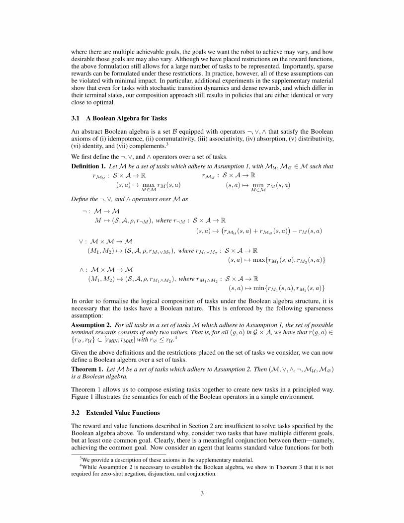
Theorem 1 allows us to compose existing tasks together to create new tasks in a principled way.Figure 1 illustrates the semantics for each of the Boolean operators in a simple environment.
3.2 Extended Value Functions
The reward and value functions described in Section 2 are insufficient to solve tasks specified by theBoolean algebra above. To understand why, consider two tasks that have multiple different goals,but at least one common goal. Clearly, there is a meaningful conjunction between them—namely,achieving the common goal. Now consider an agent that learns standard value functions for both
3We provide a description of these axioms in the supplementary material.4While Assumption 2 is necessary to establish the Boolean algebra, we show in Theorem 3 that it is not
required for zero-shot negation, disjunction, and conjunction.
3
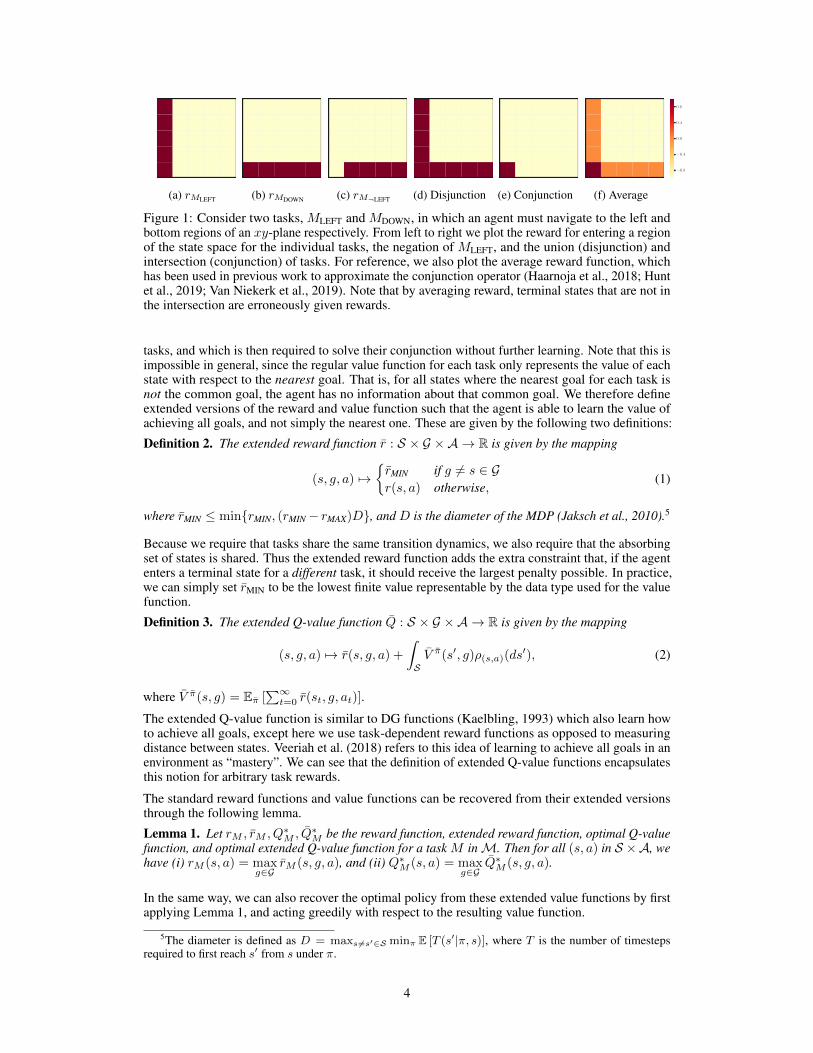
(a) rMLEFT (b) rMDOWN (c) rM¬LEFT (d) Disjunction (e) Conjunction
−0.8
−0.4
0.0
0.4
0.8
(f) Average
Figure 1: Consider two tasks, MLEFT and MDOWN, in which an agent must navigate to the left andbottom regions of an xy-plane respectively. From left to right we plot the reward for entering a regionof the state space for the individual tasks, the negation of MLEFT, and the union (disjunction) andintersection (conjunction) of tasks. For reference, we also plot the average reward function, whichhas been used in previous work to approximate the conjunction operator (Haarnoja et al., 2018; Huntet al., 2019; Van Niekerk et al., 2019). Note that by averaging reward, terminal states that are not inthe intersection are erroneously given rewards.
tasks, and which is then required to solve their conjunction without further learning. Note that this isimpossible in general, since the regular value function for each task only represents the value of eachstate with respect to the nearest goal. That is, for all states where the nearest goal for each task isnot the common goal, the agent has no information about that common goal. We therefore defineextended versions of the reward and value function such that the agent is able to learn the value ofachieving all goals, and not simply the nearest one. These are given by the following two definitions:
Definition 2. The extended reward function r̄ : S × G ×A → R is given by the mapping
(s, g, a) 7→{r̄MIN if g 6= s ∈ Gr(s, a) otherwise,
(1)
where r̄MIN ≤ min{rMIN, (rMIN− rMAX)D}, and D is the diameter of the MDP (Jaksch et al., 2010).5
Because we require that tasks share the same transition dynamics, we also require that the absorbingset of states is shared. Thus the extended reward function adds the extra constraint that, if the agententers a terminal state for a different task, it should receive the largest penalty possible. In practice,we can simply set r̄MIN to be the lowest finite value representable by the data type used for the valuefunction.
Definition 3. The extended Q-value function Q̄ : S × G ×A → R is given by the mapping
(s, g, a) 7→ r̄(s, g, a) +
∫
SV̄ π̄(s′, g)ρ(s,a)(ds
′), (2)
where V̄ π̄(s, g) = Eπ̄ [∑∞t=0 r̄(st, g, at)].
The extended Q-value function is similar to DG functions (Kaelbling, 1993) which also learn howto achieve all goals, except here we use task-dependent reward functions as opposed to measuringdistance between states. Veeriah et al. (2018) refers to this idea of learning to achieve all goals in anenvironment as “mastery”. We can see that the definition of extended Q-value functions encapsulatesthis notion for arbitrary task rewards.
The standard reward functions and value functions can be recovered from their extended versionsthrough the following lemma.
Lemma 1. Let rM , r̄M , Q∗M , Q̄∗M be the reward function, extended reward function, optimal Q-value
function, and optimal extended Q-value function for a task M inM. Then for all (s, a) in S ×A, wehave (i) rM (s, a) = max
g∈Gr̄M (s, g, a), and (ii) Q∗M (s, a) = max
g∈GQ̄∗M (s, g, a).
In the same way, we can also recover the optimal policy from these extended value functions by firstapplying Lemma 1, and acting greedily with respect to the resulting value function.
5The diameter is defined as D = maxs 6=s′∈S minπ E [T (s′|π, s)], where T is the number of timestepsrequired to first reach s′ from s under π.
4
Lemma 2. Denote S− = S \ G as the non-terminal states ofM. Let M1,M2 ∈M, and let each gin G define MDPs M1,g and M2,g with reward functions
rM1,g:= r̄M1(s, g, a) and rM2,g
:= r̄M2(s, g, a) for all (s, a) in S ×A.Then for all g in G and s in S−,
π∗g(s) ∈ arg maxa∈A
Q∗M1,g(s, a) iff π∗g(s) ∈ arg max
a∈AQ∗M2,g
(s, a).
Combining Lemmas 1 and 2, we can extract the greedy action from the extended value func-tion by first maximising over goals, and then selecting the maximising action: π∗(s) ∈arg maxa∈Amaxg∈G Q̄∗(s, g, a). If we consider the extended value function to be a set of standardvalue functions (one for each goal), then this is equivalent to first performing generalised policyimprovement (Barreto et al., 2017), and then selecting the greedy action.
Finally, much like the regular definition of value functions, the extended Q-value function can bewritten as the sum of rewards received by the agent until first encountering a terminal state.Corollary 1. Denote G∗s:g,a as the sum of rewards starting from s and taking action a up until,but not including, g. Then let M ∈ M and Q̄∗M be the extended Q-value function. Then for alls ∈ S, g ∈ G, a ∈ A, there exists a G∗s:g,a ∈ R such that
Q̄∗M (s, g, a) = G∗s:g,a + r̄M (s′, g, a′), where s′ ∈ G and a′ = arg maxb∈A
r̄M (s′, g, b).
3.3 A Boolean Algebra for Value Functions
In the same manner we constructed a Boolean algebra over a set of tasks, we can also do so for a setof optimal extended Q-value functions for the corresponding tasks.Definition 4. Let Q̄∗ be the set of optimal extended Q̄-value functions for tasks inM which adhereto Assumption 1, with Q̄∗∅, Q̄
∗U ∈ Q̄∗ the optimal Q̄-functions for the tasksM∅,MU ∈M .Define
the ¬,∨, and ∧ operators over Q̄∗ as,
¬ : Q̄∗ → Q̄∗
Q̄∗ 7→ ¬Q̄∗, where ¬Q̄∗ : S × G ×A → R(s, g, a) 7→
(Q̄∗U (s, g, a) + Q̄∗∅(s, g, a)
)− Q̄∗(s, g, a)
∨ : Q̄∗ × Q̄∗ → Q̄∗
(Q̄∗1, Q̄∗2) 7→ Q̄∗1 ∨ Q̄∗2, where Q̄∗1 ∨ Q̄∗2 : S × G ×A → R
(s, g, a) 7→ max{Q̄∗1(s, g, a), Q̄∗2(s, g, a)}∧ : Q̄∗ × Q̄∗ → Q̄∗
(Q̄∗1, Q̄∗2) 7→ Q̄∗1 ∧ Q̄∗2, where Q̄∗1 ∧ Q̄∗2 : S × G ×A → R
(s, g, a) 7→ min{Q̄∗1(s, g, a), Q̄∗2(s, g, a)}Theorem 2. Let Q̄∗ be the set of optimal extended Q̄-value functions for tasks inM which adhereto Assumption 2. Then (Q̄∗,∨,∧,¬, Q̄∗U , Q̄∗∅) is a Boolean Algebra.
3.4 Between Task and Value Function Algebras
Having established a Boolean algebra over tasks and extended value functions, we finally show thatthere exists an equivalence between the two. As a result, if we can write down a task under theBoolean algebra, we can immediately write down the optimal value function for the task.Theorem 3. Let Q̄∗ be the set of optimal extended Q̄-value functions for tasks inM which adhere toAssumption 1. Then for all M1,M2 ∈M, we have (i) Q̄∗¬M1
= ¬Q̄∗M1, (ii) Q̄∗M1∨M2
= Q̄∗M1∨ Q̄∗M2
,and (iii) Q̄∗M1∧M2
= Q̄∗M1∧ Q̄∗M2
.
Corollary 2. Let F :M→ Q̄∗ be any map fromM to Q̄∗ such that F(M) = Q̄∗M for all M inM. Then F is a homomorphism between (M,∨,∧,¬,MU ,M∅) and (Q̄∗,∨,∧,¬, Q̄∗U , Q̄∗∅).
5
Theorem 3 shows that we can provably achieve zero-shot negation, disjunction, and conjunctionprovided Assumption 1 is satisfied. Corollary 2 extends this result by showing that the task andvalue function algebras are in fact homomorphic, which implies zero-shot composition of arbitrarycombinations of negations, disjunctions, and conjunctions.
4 Zero-shot Transfer Through Composition
We can use the theory developed in the previous sections to perform zero-shot transfer by firstlearning extended value functions for a set of base tasks, and then composing them to solve newtasks expressible under the Boolean algebra. To demonstrate this, we conduct a series of experimentsin the Four Rooms domain (Sutton et al., 1999), where an agent must navigate a grid world to aparticular location. The agent can move in any of the four cardinal directions at each timestep, butcolliding with a wall leaves the agent in the same location. We add a 5th action for “stay” that theagent chooses to achieve goals. A goal position only becomes terminal if the agent chooses to stay init. The transition dynamics are deterministic, and rewards are −0.1 for all non-terminal states, and 2at the goal.
4.1 Learning Base Tasks
We use a modified version of Q-learning (Watkins, 1989) to learn the extended Q-value functionsdescribed previously. Our algorithm differs in a number of ways from standard Q-learning: we keeptrack of the set of terminating states seen so far, and at each timestep we update the extended Q-valuefunction with respect to both the current state and action, as well as all goals encountered so far. Wealso use the definition of the extended reward function, and so if the agent encounters a terminalstate of a different task, it receives reward r̄MIN. The full pseudocode is listed in the supplementarymaterial.
If we know the set of goals (and hence potential base tasks) upfront, then it is easy to select a minimalset of base tasks that can be composed to produce the largest number of composite tasks. We firstassign a Boolean label to each goal in a table, and then use the columns of the table as base tasks.The goals for each base task are then those goals with value 1 according to the table. In this domain,the two base tasks we select are MT, which requires that the agent visit either of the top two rooms,and ML, which requires visiting the two left rooms. We illustrate this selection procedure in thesupplementary material.
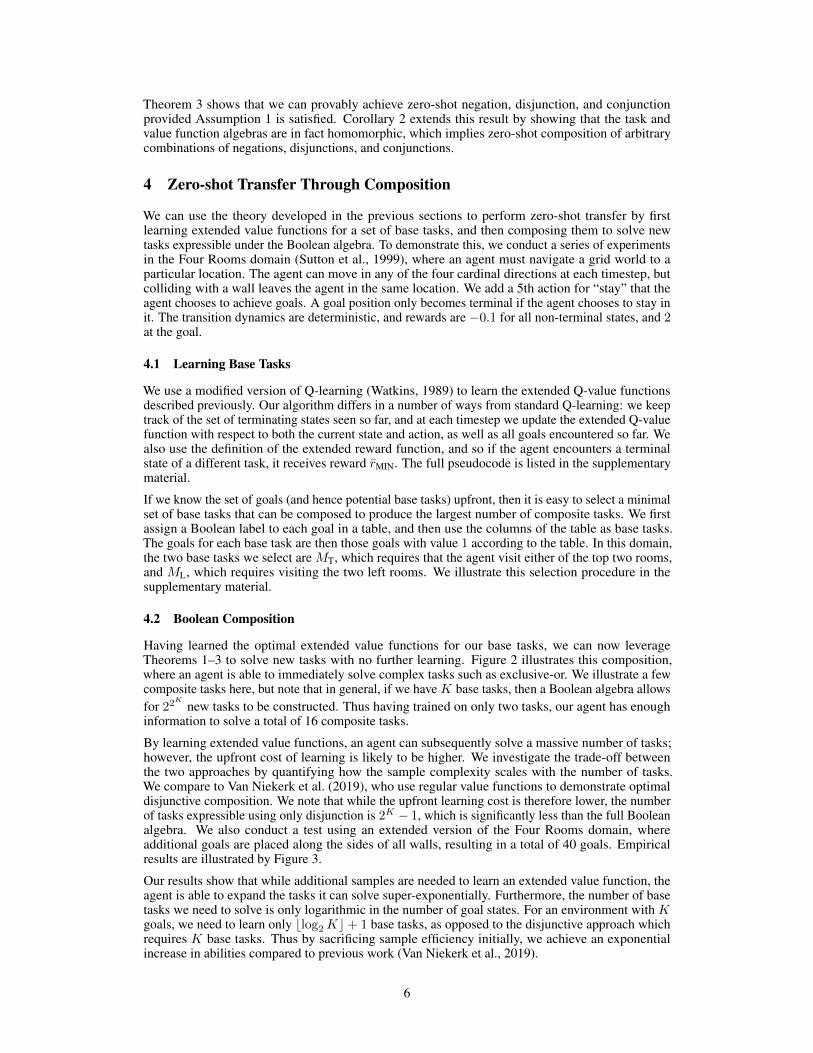
4.2 Boolean Composition
Having learned the optimal extended value functions for our base tasks, we can now leverageTheorems 1–3 to solve new tasks with no further learning. Figure 2 illustrates this composition,where an agent is able to immediately solve complex tasks such as exclusive-or. We illustrate a fewcomposite tasks here, but note that in general, if we have K base tasks, then a Boolean algebra allowsfor 22K
new tasks to be constructed. Thus having trained on only two tasks, our agent has enoughinformation to solve a total of 16 composite tasks.
By learning extended value functions, an agent can subsequently solve a massive number of tasks;however, the upfront cost of learning is likely to be higher. We investigate the trade-off betweenthe two approaches by quantifying how the sample complexity scales with the number of tasks.We compare to Van Niekerk et al. (2019), who use regular value functions to demonstrate optimaldisjunctive composition. We note that while the upfront learning cost is therefore lower, the numberof tasks expressible using only disjunction is 2K − 1, which is significantly less than the full Booleanalgebra. We also conduct a test using an extended version of the Four Rooms domain, whereadditional goals are placed along the sides of all walls, resulting in a total of 40 goals. Empiricalresults are illustrated by Figure 3.
Our results show that while additional samples are needed to learn an extended value function, theagent is able to expand the tasks it can solve super-exponentially. Furthermore, the number of basetasks we need to solve is only logarithmic in the number of goal states. For an environment with Kgoals, we need to learn only blog2Kc+ 1 base tasks, as opposed to the disjunctive approach whichrequires K base tasks. Thus by sacrificing sample efficiency initially, we achieve an exponentialincrease in abilities compared to previous work (Van Niekerk et al., 2019).
6
(a) ML (b) MT (c) ML ∨MT (d) ML ∧MT (e) ML YMT (f) ML−∨MT
Figure 2: An example of zero-shot Boolean algebraic composition using the learned extended valuefunctions. The top row shows the extended value functions. For each, the plots show the value of eachstate with respect to the four goals (the centre of each room). The bottom row shows the recoveredregular value functions obtained by maximising over goals. Arrows represent the optimal action ina given state. (a–b) The learned optimal extended value functions for the base tasks. (c) Zero-shotdisjunctive composition. (d) Zero-shot conjunctive composition. (e) Combining operators to modelexclusive-or composition. (f) Composition that produces logical nor. Note that the resulting optimalvalue function can attain a goal not explicitly represented by the base tasks.
0 2 4 6 8 10 12 14 16Number of tasks
0
1
2
3
4
5
Cum
ulat
ive
tim
este
psto
conv
erge
×105
Extended Q-function
Q-function
(a) Cumulative number of sam-ples required to learn optimal ex-tended and regular value func-tions. Error bars represent stan-dard deviations over 100 runs.
2 4 6 8 10Number of learned tasks
100
103
106
109
1012
1015
1018
Num
ber
ofso
lvab
leta
sks
Boolean task algebra
Disjunction only
No transfer
(b) Number of tasks that can besolved as a function of the numberof existing tasks solved. Resultsare plotted on a log-scale.
0 10 20 30 40 50Number of tasks
0.00
0.25
0.50
0.75
1.00
1.25
Cum
ulat
ive
tim
este
psto
conv
erge
×106
Boolean task algebra
Disjunction only
(c) Cumulative number of sam-ples required to solve tasks in a40-goal Four Rooms domain. Er-ror bars represent standard devia-tions over 100 runs.
Figure 3: Results in comparison to the disjunctive composition of Van Niekerk et al. (2019). (a) Thenumber of samples required to learn the extended value function is greater than learning a standardvalue function. However, both scale linearly and differ only by a constant factor. (b) The extendedvalue functions allow us to solve exponentially more tasks than the disjunctive approach withoutfurther learning. (c) In the modified task with 40 goals, we need to learn only 7 base tasks, as opposedto 40 for the disjunctive case.
5 Composition with Function Approximation
Finally, we demonstrate that our compositional approach can also be used to tackle high-dimensionaldomains where function approximation is required. We use the same video game environment asVan Niekerk et al. (2019), where an agent must navigate a 2D world and collect objects of differentshapes and colours from any initial position. The state space is an 84× 84 RGB image, and the agentis able to move in any of the four cardinal directions. The agent also possesses a pick-up action,which allows it to collect an object when standing on top of it. There are two shapes (squares andcircles) and three colours (blue, beige and purple) for a total of six unique objects.
To learn the extended action-value functions, we modify deep Q-learning (Mnih et al., 2015) sim-ilarly to the many-goals update method of Veeriah et al. (2018). Here, a universal value functionapproximator (UVFA) (Schaul et al., 2015) is used to represent the action values for each state and
7
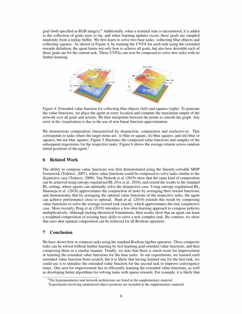
goal (both specified as RGB images).6 Additionally, when a terminal state is encountered, it is addedto the collection of goals seen so far, and when learning updates occur, these goals are sampledrandomly from a replay buffer. We first learn to solve two base tasks: collecting blue objects andcollecting squares. As shown in Figure 4, by training the UVFA for each task using the extendedrewards definition, the agent learns not only how to achieve all goals, but also how desirable each ofthose goals are for the current task. These UVFAs can now be composed to solve new tasks with nofurther learning.
Figure 4: Extended value function for collecting blue objects (left) and squares (right). To generatethe value functions, we place the agent at every location and compute the maximum output of thenetwork over all goals and actions. We then interpolate between the points to smooth the graph. Anyerror in the visualisation is due to the use of non-linear function approximation.
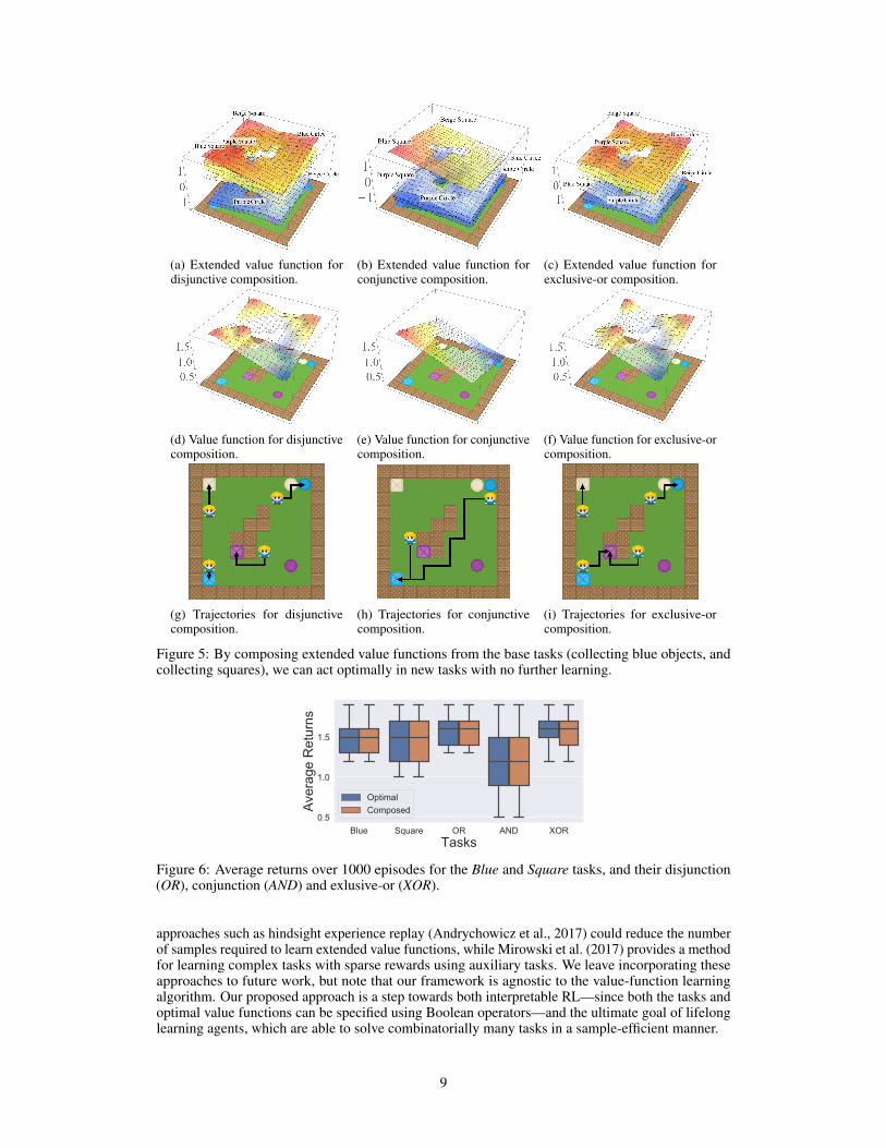
We demonstrate composition characterised by disjunction, conjunction and exclusive-or. Thiscorresponds to tasks where the target items are: (i) blue or square, (ii) blue squares, and (iii) blue orsquares, but not blue squares. Figure 5 illustrates the composed value functions and samples of thesubsequent trajectories for the respective tasks. Figure 6 shows the average returns across randominitial positions of the agent.7
6 Related Work
The ability to compose value functions was first demonstrated using the linearly-solvable MDPframework (Todorov, 2007), where value functions could be composed to solve tasks similar to thedisjunctive case (Todorov, 2009). Van Niekerk et al. (2019) show that the same kind of compositioncan be achieved using entropy-regularised RL (Fox et al., 2016), and extend the results to the standardRL setting, where agents can optimally solve the disjunctive case. Using entropy-regularised RL,Haarnoja et al. (2018) approximates the conjunction of tasks by averaging their reward functions,and demonstrates that by averaging the optimal value functions of the respective tasks, the agentcan achieve performance close to optimal. Hunt et al. (2019) extends this result by composingvalue functions to solve the average reward task exactly, which approximates the true conjunctivecase. More recently, Peng et al. (2019) introduce a few-shot learning approach to compose policiesmultiplicatively. Although lacking theoretical foundations, their results show that an agent can learna weighted composition of existing base skills to solve a new complex task. By contrast, we showthat zero-shot optimal composition can be achieved for all Boolean operators.
7 Conclusion
We have shown how to compose tasks using the standard Boolean algebra operators. These compositetasks can be solved without further learning by first learning goal-oriented value functions, and thencomposing them in a similar manner. Finally, we note that there is much room for improvementin learning the extended value functions for the base tasks. In our experiments, we learned eachextended value function from scratch, but it is likely that having learned one for the first task, wecould use it to initialise the extended value function for the second task to improve convergencetimes. One area for improvement lies in efficiently learning the extended value functions, as wellas developing better algorithms for solving tasks with sparse rewards. For example, it is likely that
6The hyperparameters and network architecture are listed in the supplementary material7Experiments involving randomised object positions are included in the supplementary material.
8
(a) Extended value function fordisjunctive composition.
(b) Extended value function forconjunctive composition.
(c) Extended value function forexclusive-or composition.
(d) Value function for disjunctivecomposition.
(e) Value function for conjunctivecomposition.
(f) Value function for exclusive-orcomposition.
(g) Trajectories for disjunctivecomposition.
(h) Trajectories for conjunctivecomposition.
(i) Trajectories for exclusive-orcomposition.
Figure 5: By composing extended value functions from the base tasks (collecting blue objects, andcollecting squares), we can act optimally in new tasks with no further learning.
Blue Square OR AND XORTasks
0.5
1.0
1.5
Aver
age
Ret
urns
OptimalComposed
Figure 6: Average returns over 1000 episodes for the Blue and Square tasks, and their disjunction(OR), conjunction (AND) and exlusive-or (XOR).
approaches such as hindsight experience replay (Andrychowicz et al., 2017) could reduce the numberof samples required to learn extended value functions, while Mirowski et al. (2017) provides a methodfor learning complex tasks with sparse rewards using auxiliary tasks. We leave incorporating theseapproaches to future work, but note that our framework is agnostic to the value-function learningalgorithm. Our proposed approach is a step towards both interpretable RL—since both the tasks andoptimal value functions can be specified using Boolean operators—and the ultimate goal of lifelonglearning agents, which are able to solve combinatorially many tasks in a sample-efficient manner.
9
Broader Impact
Our work is mainly theoretical, but is a step towards creating agents that can solve tasks specifiedusing human-understandable Boolean expressions, which could one day be deployed in practical RLsystems. We envisage this as an avenue for overcoming the problem of reward misspecification, andfor developing safer agents whose goals are readily interpretable by humans.
Acknowledgments and Disclosure of Funding
The authors wish to thank the anonymous reviewers for their helpful comments, and Pieter Abbeel,Marc Deisenroth and Shakir Mohamed for their assistance in reviewing a final draft of this paper.This work is based on the research supported in part by the National Research Foundation of SouthAfrica (Grant Number: 17808).
ReferencesAndrychowicz, M., Wolski, F., Ray, A., Schneider, J., Fong, R., Welinder, P., McGrew, B., Tobin,
J., Abbeel, P., and Zaremba, W. Hindsight experience replay. In Advances in Neural InformationProcessing Systems, pp. 5048–5058, 2017.
Barreto, A., Dabney, W., Munos, R., Hunt, J., Schaul, T., van Hasselt, H., and Silver, D. Successorfeatures for transfer in reinforcement learning. In Advances in Neural Information ProcessingSystems, pp. 4055–4065, 2017.
Barto, A. and Mahadevan, S. Recent advances in hierarchical reinforcement learning. Discrete EventDynamic Systems, 13(1-2):41–77, 2003.
Bertsekas, D. and Tsitsiklis, J. An analysis of stochastic shortest path problems. Mathematics ofOperations Research, 16(3):580–595, 1991.
Fox, R., Pakman, A., and Tishby, N. Taming the noise in reinforcement learning via soft updates. In32nd Conference on Uncertainty in Artificial Intelligence, 2016.
Haarnoja, T., Pong, V., Zhou, A., Dalal, M., Abbeel, P., and Levine, S. Composable deep reinforce-ment learning for robotic manipulation. In 2018 IEEE International Conference on Robotics andAutomation, pp. 6244–6251. IEEE, 2018.
Hunt, J., Barreto, A., Lillicrap, T., and Heess, N. Composing entropic policies using divergencecorrection. In Proceedings of the 36th International Conference on Machine Learning, volume 97of Proceedings of Machine Learning Research, pp. 2911–2920. PMLR, 2019.
Jaksch, T., Ortner, R., and Auer, P. Near-optimal regret bounds for reinforcement learning. Journalof Machine Learning Research, 11(Apr):1563–1600, 2010.
James, H. and Collins, E. An analysis of transient Markov decision processes. Journal of AppliedProbability, 43(3):603–621, 2006.
Kaelbling, L. P. Learning to achieve goals. In International Joint Conferences on Artificial Intelli-gence, pp. 1094–1099, 1993.
Levine, S., Finn, C., Darrell, T., and Abbeel, P. End-to-end training of deep visuomotor policies. TheJournal of Machine Learning Research, 17(1):1334–1373, 2016.
Lillicrap, T., Hunt, J., Pritzel, A., Heess, N., Erez, T., Tassa, Y., Silver, D., and Wierstra, D.Continuous control with deep reinforcement learning. In International Conference on LearningRepresentations, 2016.
Mirowski, P., Pascanu, R., Viola, F., Soyer, H., Ballard, A., Banino, A., Denil, M., Goroshin, R.,Sifre, L., Kavukcuoglu, K., et al. Learning to navigate in complex environments. In InternationalConference on Learning Representations, 2017.
10
Mnih, V., Kavukcuoglu, K., Silver, D., Rusu, A., Veness, J., Bellemare, M., Graves, A., Riedmiller,M., Fidjeland, A., Ostrovski, G., et al. Human-level control through deep reinforcement learning.Nature, 518(7540):529, 2015.
Peng, X., Chang, M., Zhang, G., Abbeel, P., and Levine, S. MCP: Learning composable hierarchicalcontrol with multiplicative compositional policies. arXiv preprint arXiv:1905.09808, 2019.
Saxe, A., Earle, A., and Rosman, B. Hierarchy through composition with multitask LMDPs.Proceedings of the 34th International Conference on Machine Learning, 70:3017–3026, 2017.
Schaul, T., Horgan, D., Gregor, K., and Silver, D. Universal value function approximators. InProceedings of the 32nd International Conference on Machine Learning, volume 37 of Proceedingsof Machine Learning Research, pp. 1312–1320, Lille, France, 2015. PMLR.
Silver, D., Schrittwieser, J., Simonyan, K., Antonoglou, I., Huang, A., Guez, A., Hubert, T., Baker,L., Lai, M., Bolton, A., et al. Mastering the game of go without human knowledge. Nature, 550(7676):354, 2017.
Sutton, R., Precup, D., and Singh, S. Between MDPs and semi-MDPs: A framework for temporalabstraction in reinforcement learning. Artificial Intelligence, 112(1-2):181–211, 1999.
Todorov, E. Linearly-solvable Markov decision problems. In Advances in Neural InformationProcessing Systems, pp. 1369–1376, 2007.
Todorov, E. Compositionality of optimal control laws. In Advances in Neural Information ProcessingSystems, pp. 1856–1864, 2009.
Van Niekerk, B., James, S., Earle, A., and Rosman, B. Composing value functions in reinforcementlearning. In Proceedings of the 36th International Conference on Machine Learning, volume 97 ofProceedings of Machine Learning Research, pp. 6401–6409. PMLR, 2019.
Veeriah, V., Oh, J., and Singh, S. Many-goals reinforcement learning. arXiv preprintarXiv:1806.09605, 2018.
Watkins, C. Learning from delayed rewards. PhD thesis, King’s College, Cambridge, 1989.
11
Supplementary Material:A Boolean Task Algebra For Reinforcement Learning
Geraud Nangue Tasse, Steven James, Benjamin RosmanSchool of Computer Science and Applied Mathematics
University of the WitwatersrandJohannesburg, South Africa
[email protected], {steven.james, benjamin.rosman1}@wits.ac.za
1 Boolean Algebra Definition
Definition 1. A Boolean algebra is a set B equipped with the binary operators ∨ (disjunction) and ∧(conjunction), and the unary operator ¬ (negation), which satisfies the following Boolean algebraaxioms for a, b, c in B:
(i) Idempotence: a ∧ a = a ∨ a = a.
(ii) Commutativity: a ∧ b = b ∧ a and a ∨ b = b ∨ a.
(iii) Associativity: a ∧ (b ∧ c) = (a ∧ b) ∧ c and a ∧ (b ∨ c) = (a ∨ b) ∨ c.
(iv) Absorption: a ∧ (a ∨ b) = a ∨ (a ∧ b) = a.
(v) Distributivity: a ∧ (b ∨ c) = (a ∧ b) ∨ (a ∧ c) and a ∨ (b ∧ c) = (a ∨ b) ∧ (a ∨ c).
(vi) Identity: there exists 0,1 in B such that
0 ∧ a = 0
0 ∨ a = a
1 ∧ a = a
1 ∨ a = 1
(vii) Complements: for every a in B, there exists an element a′ in B such that a ∧ a′ = 0 anda ∨ a′ = 1.
2 Proof for Boolean Task Algebra
Theorem 1. LetM be a set of tasks which adhere to Assumption 2. Then (M,∨,∧,¬,MU ,M∅)is a Boolean algebra.
Proof. Let M1,M2 ∈M. We show that ¬,∨,∧ satisfy the Boolean properties (i) – (vii).
(i)–(v): These easily follow from the fact that the min and max functions satisfy the idempotent,commutative, associative, absorption and distributive laws.
34th Conference on Neural Information Processing Systems (NeurIPS 2020), Vancouver, Canada.
arX
iv:2
001.
0139
4v2
[cs
.LG
] 1
5 O
ct 2
020
(vi): Let rMU∧M1 and rM1 be the reward functions forMU ∧M1 and M1 respectively. Then forall (s, a) in S ×A,
rMU∧M1(s, a) =
{min{rU , rM1
(s, a)}, if s ∈ Gmin{rs,a, rs,a}, otherwise.
=
{rM1
(s, a), if s ∈ Grs,a, otherwise.
(rM1(s, a) ∈ {r∅, rU} for s ∈ G)
= rM1(s, a).
ThusMU∧M1 = M1. SimilarlyMU∨M1 =MU ,M∅∧M1 =M∅, andM∅∨M1 = M1
. HenceM∅ andMU are the universal bounds ofM.
(vii): Let rM1∧¬M1 be the reward function for M1 ∧ ¬M1. Then for all (s, a) in S ×A,
rM1∧¬M1(s, a) =
{min{rM1
(s, a), (rU + r∅)− rM1(s, a)}, if s ∈ G
min{rs,a, (rs,a + rs,a)− rs,a}, otherwise.
=
r∅, if s ∈ G and rM1(s, a) = rU
r∅, if s ∈ G and rM1(s, a) = r∅rs,a, otherwise.
= rM∅(s, a).
Thus M1 ∧ ¬M1 =M∅, and similarly M1 ∨ ¬M1 =MU .
3 Proofs of Properties of Extended Value Functions
Lemma 1. Let rM , r̄M , Q∗M , Q̄∗M be the reward function, extended reward function, optimal Q-value
function, and optimal extended Q-value function for a task M inM. Then for all (s, a) in S ×A, wehave (i) rM (s, a) = max
g∈Gr̄M (s, g, a), and (ii) Q∗M (s, a) = max
g∈GQ̄∗M (s, g, a).
Proof.
(i):
maxg∈G
r̄M (s, g, a) =
{max{r̄MIN, rM (s, a)}, if s ∈ Gmaxg∈G
rM (s, a), otherwise.
= rM (s, a) (r̄MIN ≤ rMIN ≤ rM (s, a) by definition).
(ii): Each g in G can be thought of as defining an MDP Mg := (S,A, ρ, rMg) with reward function
rMg (s, a) := r̄M (s, g, a) and optimal Q-value function Q∗Mg(s, a) = Q̄∗M (s, g, a). Then using
(i) we have rM (s, a) = maxg∈G
rMg (s, a) and from Van Niekerk et al. (2019, Corollary 1), we have
that Q∗M (s, a) = maxg∈G
Q∗Mg(s, a) = max
g∈GQ̄∗M (s, g, a).
Lemma 2. Denote S− = S \ G as the non-terminal states ofM. Let M1,M2 ∈M, and let each gin G define MDPs M1,g and M2,g with reward functions
rM1,g:= r̄M1(s, g, a) and rM2,g
:= r̄M2(s, g, a) for all (s, a) in S ×A.
Then for all g in G and s in S−,
π∗g(s) ∈ arg maxa∈A
Q∗M1,g(s, a) iff π∗g(s) ∈ arg max
a∈AQ∗M2,g
(s, a).
2
Proof. Let g ∈ G, s ∈ S− and let π∗g be defined by
π∗g(s′) ∈ arg maxa∈A
Q∗M1,g(s, a) for all s′ ∈ S.
If g is unreachable from s, then we are done since for all (s′, a) in S ×A we have
g 6= s′ =⇒ rM1,g(s′, a) =
{r̄MIN, if s′ ∈ Grs′,a, otherwise
= rM2,g(s′, a)
=⇒ M1,g = M2,g.
If g is reachable from s, then we show that following π∗g must reach g. Since π∗g is proper, it mustreach a terminal state g′ ∈ G. Assume g′ 6= g. Let πg be a policy that produces the shortest trajectoryto g. Let Gπ
∗g and Gπg be the returns for the respective policies. Then,
Gπ∗g ≥ Gπg
=⇒ Gπ∗gT−1 + rM1,g
(g′, π∗g(g′)) ≥ Gπg ,
where Gπ∗gT−1 =
T−1∑
t=0
rM1,g(st, π
∗g(st)) and T is the time at which g′ is reached.
=⇒ Gπ∗gT−1 + r̄MIN ≥ Gπg , since g 6= g′ ∈ G
=⇒ r̄MIN ≥ Gπg −Gπ∗g
T−1
=⇒ (rMIN − rMAX)D ≥ Gπg −Gπ∗g
T−1, by definition of r̄MIN
=⇒ Gπ∗gT−1 − rMAXD ≥ Gπg − rMIND, since Gπg ≥ rMIND
=⇒ Gπ∗gT−1 − rMAXD ≥ 0
=⇒ Gπ∗gT−1 ≥ rMAXD.
But this is a contradiction since the result obtained by following an optimal trajectory up to a terminalstate without the reward for entering the terminal state must be strictly less that receiving rMAX forevery step of the longest possible optimal trajectory. Hence we must have g′ = g. Similarly, alloptimal policies of M2,g must reach g. Hence π∗g(s) ∈ arg max
a∈AQ∗M2,g
(s, a). Since M1 and M2 are
arbitrary elements ofM, the reverse implication holds too.
Corollary 1. Denote G∗s:g,a as the sum of rewards starting from s and taking action a up until,but not including, g. Then let M ∈ M and Q̄∗M be the extended Q-value function. Then for alls ∈ S, g ∈ G, a ∈ A, there exists a G∗s:g,a ∈ R such that
Q̄∗M (s, g, a) = G∗s:g,a + r̄M (s′, g, a′), where s′ ∈ G and a′ = arg maxb∈A
r̄M (s′, g, b).
Proof. This follows directly from Lemma 2. Since all tasks M ∈M share the same optimal policyπ∗g up to (but not including) the goal state g ∈ G, their return G
π∗gT−1 =
∑T−1t=0 rM (st, π
∗g(st)) is the
same up to (but not including) g.
4 Proof for Boolean Extendend Value Functions Algebra
Theorem 2. Let Q̄∗ be the set of optimal extended Q̄-value functions for tasks inM which adhereto Assumption 2. Then (Q̄∗,∨,∧,¬, Q̄∗U , Q̄∗∅) is a Boolean Algebra.
Proof. Let Q̄∗M1, Q̄∗M2
∈ Q̄∗ be the optimal Q̄-value functions for tasks M1,M2 ∈M with rewardfunctions rM1
and rM2. We show that ¬,∨,∧ satisfy the Boolean properties (i) – (vii).
3
(i)–(v): These follow directly from the properties of the min and max functions.
(vi): For all (s, g, a) in S × G ×A,(Q̄∗U ∧ Q̄∗M1
)(s, g, a) = min{(Q̄∗U (s, g, a), Q̄∗M1(s, g, a)}
= min{G∗s:g,a + r̄MU (s′, g, a′), G∗s:g,a + r̄M1(s′, g, a′)} (Corollary 1)
= G∗s:g,a + min{r̄MU (s′, g, a′), r̄M1(s′, g, a′)}
= G∗s:g,a + r̄M1(s′, g, a′) (since r̄M1
(s′, g, a′) ∈ {r∅, rU , r̄MIN})= Q̄∗M1
(s, g, a).
Similarly, Q̄∗U ∨ Q̄∗M1= Q̄∗U , Q̄
∗∅ ∧ Q̄∗M1
= Q̄∗∅, and Q̄∗∅ ∨ Q̄∗M1= Q̄∗M1
.
(vii): For all (s, g, a) in S × G ×A,(Q̄∗M1
∧ ¬Q̄∗M1)(s, g, a) = min{Q̄∗M1
(s, g, a), (Q̄∗U (s, g, a)− Q̄∗∅(s, g, a))− Q̄∗M1(s, g, a)}
= G∗s:g,a + min{r̄M1(s′, g, a′), (r̄MU (s′, g, a′) + r̄M∅(s′, g, a′))
− r̄M1(s′, g, a′)}= G∗s:g,a + r̄M∅(s′, g, a′)
= Q̄∗∅(s, g, a).
Similarly, Q̄∗M1∨ ¬Q̄∗M1
= Q̄∗U .
5 Proof for Zero-shot Composition
Theorem 3. Let Q̄∗ be the set of optimal extended Q̄-value functions for tasks inM which adhere toAssumption 1. Then for all M1,M2 ∈M, we have (i) Q̄∗¬M1
= ¬Q̄∗M1, (ii) Q̄∗M1∨M2
= Q̄∗M1∨ Q̄∗M2
,and (iii) Q̄∗M1∧M2
= Q̄∗M1∧ Q̄∗M2
.
Proof. Let M1,M2 ∈M. Then for all (s, g, a) in S × G ×A,
(i):Q̄∗¬M1
(s, g, a) = G∗s:g,a + r̄¬M1(s′, g, a′) (from Corollary 1)
= G∗s:g,a + (r̄MU (s′, g, a′) + r̄M∅(s′, g, a′))− r̄M1(s′, g, a′)
=[(G∗s:g,a + r̄MU (s′, g, a′)) + (G∗s:g,a + r̄M∅(s′, g, a′))
]− (G∗s:g,a + r̄M1
(s′, g, a′))
=[Q̄∗U (s, g, a) + Q̄∗∅(s, g, a)
]− Q̄∗M1
(s, g, a)
= ¬Q̄∗M1(s, g, a)
(ii):Q̄∗M1∨M2
(s, g, a) = G∗s:g,a + r̄M1∨M2(s′, g, a′)
= G∗s:g,a + max{r̄M1(s′, g, a′), r̄M2(s′, g, a′′)}= max{G∗s:g,a + r̄M1(s′, g, a′), G∗s:g,a + r̄M2(s′, g, a′′)}= max{Q̄∗M1
(s, g, a), Q̄∗M2(s, g, a)}
= (Q̄∗M1∨ Q̄∗M2
)(s, g, a)
(iii): Follows similarly to (ii).
Corollary 2. Let F :M→ Q̄∗ be any map fromM to Q̄∗ such that F(M) = Q̄∗M for all M inM. Then F is a homomorphism between (M,∨,∧,¬,MU ,M∅) and (Q̄∗,∨,∧,¬, Q̄∗U , Q̄∗∅).
Proof. This follows from Theorem 3.
4
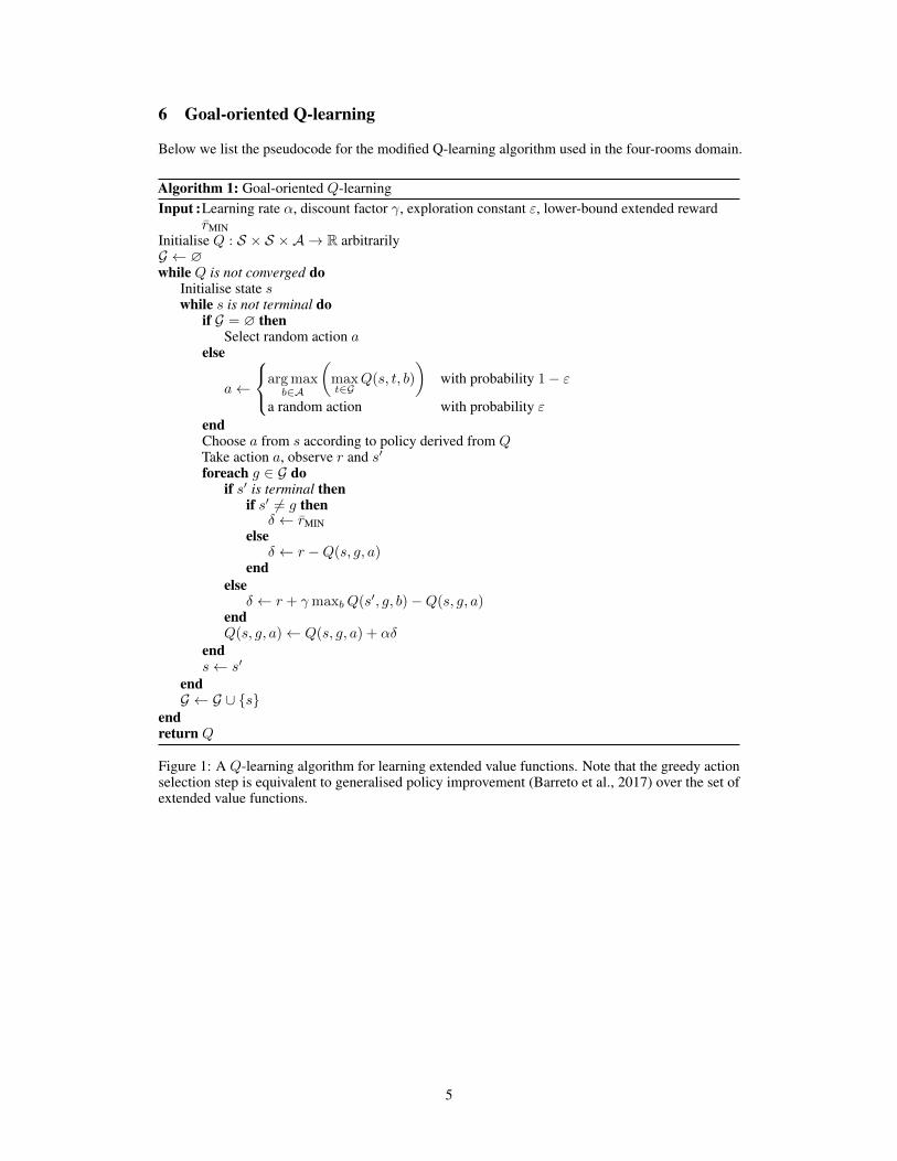
6 Goal-oriented Q-learning
Below we list the pseudocode for the modified Q-learning algorithm used in the four-rooms domain.
Algorithm 1: Goal-oriented Q-learningInput :Learning rate α, discount factor γ, exploration constant ε, lower-bound extended reward
r̄MINInitialise Q : S × S ×A → R arbitrarilyG ← ∅while Q is not converged do
Initialise state swhile s is not terminal do
if G = ∅ thenSelect random action a
else
a←
arg maxb∈A
(maxt∈G
Q(s, t, b)
)with probability 1− ε
a random action with probability εendChoose a from s according to policy derived from QTake action a, observe r and s′foreach g ∈ G do
if s′ is terminal thenif s′ 6= g then
δ ← r̄MINelse
δ ← r −Q(s, g, a)end
elseδ ← r + γmaxbQ(s′, g, b)−Q(s, g, a)
endQ(s, g, a)← Q(s, g, a) + αδ
ends← s′
endG ← G ∪ {s}
endreturn Q
Figure 1: A Q-learning algorithm for learning extended value functions. Note that the greedy actionselection step is equivalent to generalised policy improvement (Barreto et al., 2017) over the set ofextended value functions.
5
7 Investigating Practical Considerations
The theoretical results presented in this work rely on Assumptions 1 and 2, which restrict the tasks’transition dynamics and reward functions in potentially problematic ways. Although this is necessaryto prove that Boolean algebraic composition results in optimal value functions, in this section weinvestigate whether these can be practically ignored. In particular, we investigate three restrictions:(i) the requirement that tasks share the same terminal states, (ii) the impact of using dense rewards,and (iii) the requirement that tasks have deterministic transition dynamics.
7.1 Four Rooms Experiments
We use the same setup as the experiment outlined in Section 4. We first investigate the differencebetween using sparse and dense rewards. Our sparse reward function is defined as
rsparse(s, a) =
{2 if s ∈ G−0.1 otherwise,
and we use a dense reward function similar to Peng et al. (2019):
rdense(s, a) =0.1
|G|∑
g∈Gexp(−|s− g|
2
4) + rsparse(s, a)
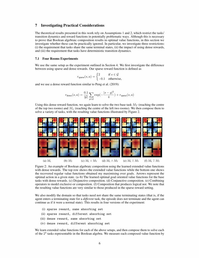
Using this dense reward function, we again learn to solve the two base task MT (reaching the centreof the top two rooms) and ML (reaching the centre of the left two rooms). We then compose them tosolve a variety of tasks, with the resulting value functions illustrated by Figure 2.
(a) ML (b) MT (c) ML ∨MT (d) ML ∧MT (e) ML YMT (f) ML−∨MT
Figure 2: An example of Boolean algebraic composition using the learned extended value functionswith dense rewards. The top row shows the extended value functions while the bottom one showsthe recovered regular value functions obtained my maximising over goals. Arrows represent theoptimal action in a given state. (a–b) The learned optimal goal oriented value functions for the basetasks with dense rewards. (c) Disjunctive composition. (d) Conjunctive composition. (e) Combiningoperators to model exclusive-or composition. (f) Composition that produces logical nor. We note thatthe resulting value functions are very similar to those produced in the sparse reward setting.
We also modify the domain so that tasks need not share the same terminating states (that is, if theagent enters a terminating state for a different task, the episode does not terminate and the agent cancontinue as if it were a normal state). This results in four versions of the experiment:
(i) sparse reward, same absorbing set(ii) sparse reward, different absorbing set
(iii) dense reward, same absorbing set(iv) dense reward, different absorbing set
We learn extended value functions for each of the above setups, and then compose them to solve eachof the 24 tasks representable in the Boolean algebra. We measure each composed value function by
6
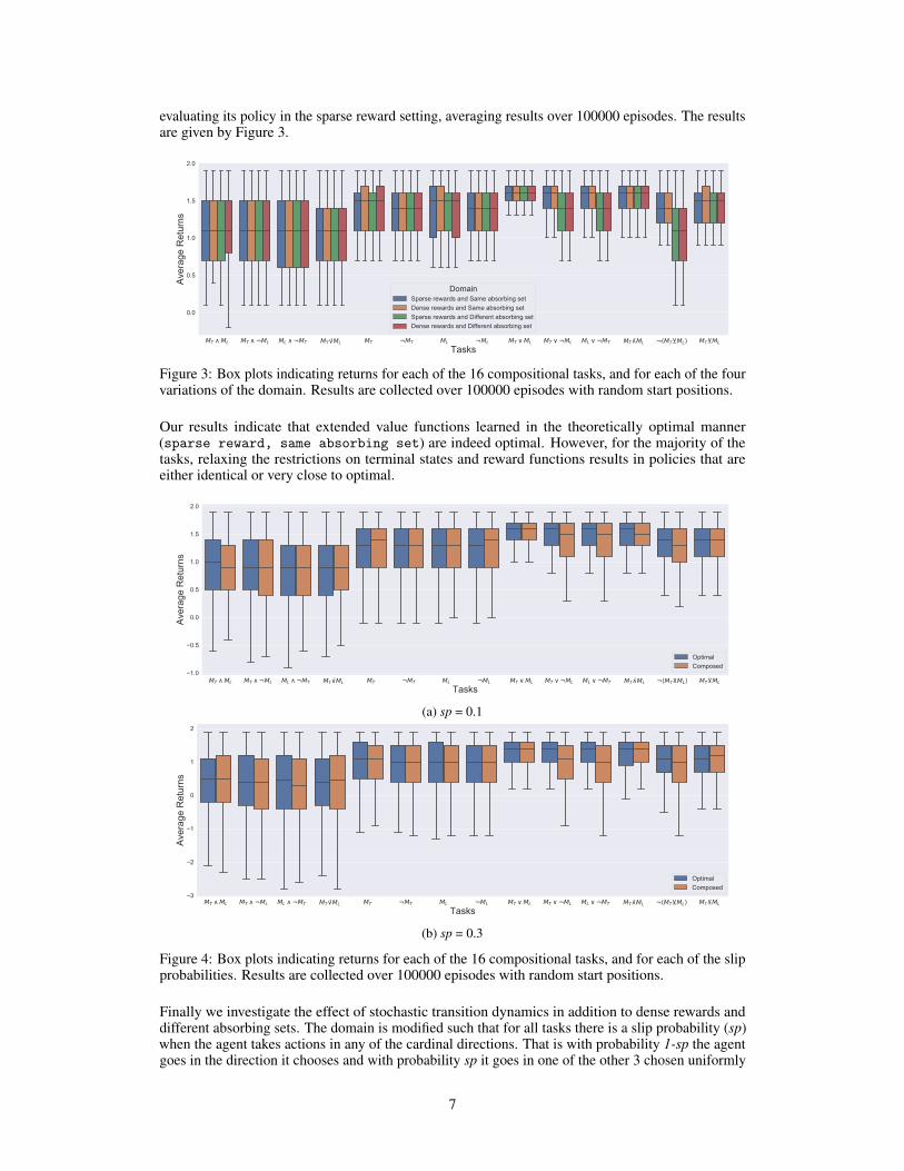
evaluating its policy in the sparse reward setting, averaging results over 100000 episodes. The resultsare given by Figure 3.
MT ML MT ¬ML ML ¬MT MT ML MT ¬MT ML ¬ML MT ML MT ¬ML ML ¬MT MT ML ¬(MT ML) MT ML
Tasks
0.0
0.5
1.0
1.5
2.0
Aver
age
Ret
urns
DomainSparse rewards and Same absorbing setDense rewards and Same absorbing setSparse rewards and Different absorbing setDense rewards and Different absorbing set
Figure 3: Box plots indicating returns for each of the 16 compositional tasks, and for each of the fourvariations of the domain. Results are collected over 100000 episodes with random start positions.
Our results indicate that extended value functions learned in the theoretically optimal manner(sparse reward, same absorbing set) are indeed optimal. However, for the majority of thetasks, relaxing the restrictions on terminal states and reward functions results in policies that areeither identical or very close to optimal.
MT ML MT ¬ML ML ¬MT MT ML MT ¬MT ML ¬ML MT ML MT ¬ML ML ¬MT MT ML ¬(MT ML) MT ML
Tasks
1.0
0.5
0.0
0.5
1.0
1.5
2.0
Aver
age
Ret
urns
OptimalComposed
(a) sp = 0.1
MT ML MT ¬ML ML ¬MT MT ML MT ¬MT ML ¬ML MT ML MT ¬ML ML ¬MT MT ML ¬(MT ML) MT ML
Tasks
3
2
1
0
1
2
Aver
age
Ret
urns
OptimalComposed
(b) sp = 0.3
Figure 4: Box plots indicating returns for each of the 16 compositional tasks, and for each of the slipprobabilities. Results are collected over 100000 episodes with random start positions.
Finally we investigate the effect of stochastic transition dynamics in addition to dense rewards anddifferent absorbing sets. The domain is modified such that for all tasks there is a slip probability (sp)when the agent takes actions in any of the cardinal directions. That is with probability 1-sp the agentgoes in the direction it chooses and with probability sp it goes in one of the other 3 chosen uniformly
7
at random. The results are given in Figure 4. Our results show that even when the transition dynamicsare stochastic, the learned extended value functions can be composed to produce policies that areidentical or very close to optimal.
In summary, we have shown that our compositional approach offers strong empirical performance,even when the theoretical assumptions are violated.
7.2 Function Approximation Experiments
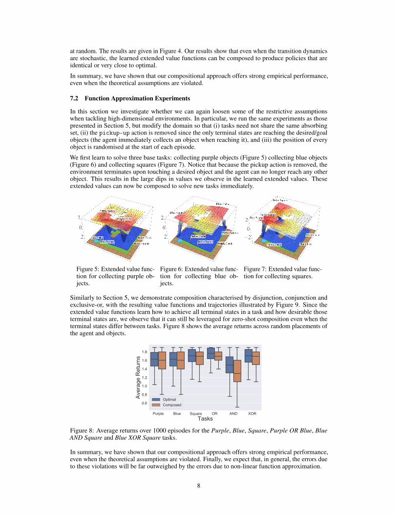
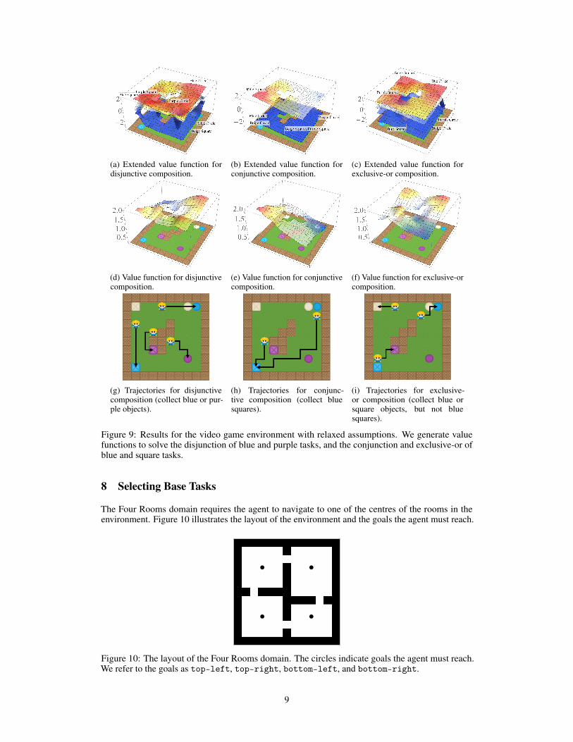
In this section we investigate whether we can again loosen some of the restrictive assumptionswhen tackling high-dimensional environments. In particular, we run the same experiments as thosepresented in Section 5, but modify the domain so that (i) tasks need not share the same absorbingset, (ii) the pickup-up action is removed since the only terminal states are reaching the desired/goalobjects (the agent immediately collects an object when reaching it), and (iii) the position of everyobject is randomised at the start of each episode.
We first learn to solve three base tasks: collecting purple objects (Figure 5) collecting blue objects(Figure 6) and collecting squares (Figure 7). Notice that because the pickup action is removed, theenvironment terminates upon touching a desired object and the agent can no longer reach any otherobject. This results in the large dips in values we observe in the learned extended values. Theseextended values can now be composed to solve new tasks immediately.
Figure 5: Extended value func-tion for collecting purple ob-jects.
Figure 6: Extended value func-tion for collecting blue ob-jects.
Figure 7: Extended value func-tion for collecting squares.
Similarly to Section 5, we demonstrate composition characterised by disjunction, conjunction andexclusive-or, with the resulting value functions and trajectories illustrated by Figure 9. Since theextended value functions learn how to achieve all terminal states in a task and how desirable thoseterminal states are, we observe that it can still be leveraged for zero-shot composition even when theterminal states differ between tasks. Figure 8 shows the average returns across random placements ofthe agent and objects.
Purple Blue Square OR AND XORTasks
0.6
0.8
1.0
1.2
1.4
1.6
1.8
Aver
age
Ret
urns
OptimalComposed
Figure 8: Average returns over 1000 episodes for the Purple, Blue, Square, Purple OR Blue, BlueAND Square and Blue XOR Square tasks.
In summary, we have shown that our compositional approach offers strong empirical performance,even when the theoretical assumptions are violated. Finally, we expect that, in general, the errors dueto these violations will be far outweighed by the errors due to non-linear function approximation.
8
(a) Extended value function fordisjunctive composition.
(b) Extended value function forconjunctive composition.
(c) Extended value function forexclusive-or composition.
(d) Value function for disjunctivecomposition.
(e) Value function for conjunctivecomposition.
(f) Value function for exclusive-orcomposition.
(g) Trajectories for disjunctivecomposition (collect blue or pur-ple objects).
(h) Trajectories for conjunc-tive composition (collect bluesquares).
(i) Trajectories for exclusive-or composition (collect blue orsquare objects, but not bluesquares).
Figure 9: Results for the video game environment with relaxed assumptions. We generate valuefunctions to solve the disjunction of blue and purple tasks, and the conjunction and exclusive-or ofblue and square tasks.
8 Selecting Base Tasks
The Four Rooms domain requires the agent to navigate to one of the centres of the rooms in theenvironment. Figure 10 illustrates the layout of the environment and the goals the agent must reach.
Figure 10: The layout of the Four Rooms domain. The circles indicate goals the agent must reach.We refer to the goals as top-left, top-right, bottom-left, and bottom-right.
9
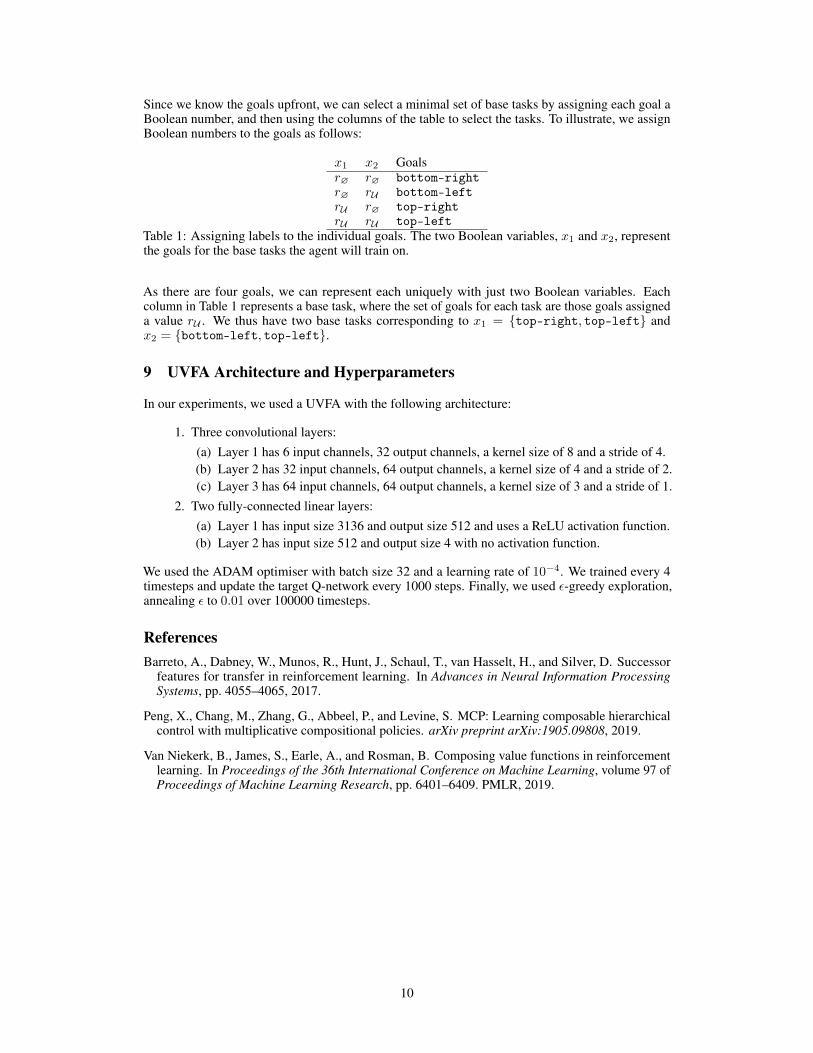
Since we know the goals upfront, we can select a minimal set of base tasks by assigning each goal aBoolean number, and then using the columns of the table to select the tasks. To illustrate, we assignBoolean numbers to the goals as follows:
x1 x2 Goalsr∅ r∅ bottom-rightr∅ rU bottom-leftrU r∅ top-rightrU rU top-left
Table 1: Assigning labels to the individual goals. The two Boolean variables, x1 and x2, representthe goals for the base tasks the agent will train on.
As there are four goals, we can represent each uniquely with just two Boolean variables. Eachcolumn in Table 1 represents a base task, where the set of goals for each task are those goals assigneda value rU . We thus have two base tasks corresponding to x1 = {top-right, top-left} andx2 = {bottom-left, top-left}.
9 UVFA Architecture and Hyperparameters
In our experiments, we used a UVFA with the following architecture:
1. Three convolutional layers:(a) Layer 1 has 6 input channels, 32 output channels, a kernel size of 8 and a stride of 4.(b) Layer 2 has 32 input channels, 64 output channels, a kernel size of 4 and a stride of 2.(c) Layer 3 has 64 input channels, 64 output channels, a kernel size of 3 and a stride of 1.
2. Two fully-connected linear layers:(a) Layer 1 has input size 3136 and output size 512 and uses a ReLU activation function.(b) Layer 2 has input size 512 and output size 4 with no activation function.
We used the ADAM optimiser with batch size 32 and a learning rate of 10−4. We trained every 4timesteps and update the target Q-network every 1000 steps. Finally, we used ε-greedy exploration,annealing ε to 0.01 over 100000 timesteps.
ReferencesBarreto, A., Dabney, W., Munos, R., Hunt, J., Schaul, T., van Hasselt, H., and Silver, D. Successor
features for transfer in reinforcement learning. In Advances in Neural Information ProcessingSystems, pp. 4055–4065, 2017.
Peng, X., Chang, M., Zhang, G., Abbeel, P., and Levine, S. MCP: Learning composable hierarchicalcontrol with multiplicative compositional policies. arXiv preprint arXiv:1905.09808, 2019.
Van Niekerk, B., James, S., Earle, A., and Rosman, B. Composing value functions in reinforcementlearning. In Proceedings of the 36th International Conference on Machine Learning, volume 97 ofProceedings of Machine Learning Research, pp. 6401–6409. PMLR, 2019.
10