Embed Size (px)
Citation preview

ARTICLE
A bivariate geometric distribution allowing for positive or negative
correlation
Alessandro Barbieroa
aDepartment of Economics, Management and Quantitative Methods, Universita degli Studi
di Milano, 20122 Milan, Italy
ARTICLE HISTORY
Compiled May 1, 2018
Abstract
In this paper, we propose a new bivariate geometric model, derived by linking two
univariate geometric distributions through a specific copula function, allowing for
positive and negative correlations. Some properties of this joint distribution are pre-
sented and discussed, with particular reference to attainable correlations, conditional
distributions, reliability concepts, and parameter estimation. A Monte Carlo simu-
lation study empirically evaluates and compares the performance of the proposed
estimators in terms of bias and standard error. Finally, in order to demonstrate its
usefulness, the model is applied to a real data set.
KEYWORDS
attainable correlations; correlated counts; Farlie-Gumbel-Morgenstern copula;
method of moments; two-step maximum likelihood
1. INTRODUCTION
In recent years, the construction of bivariate (and multivariate) discrete distributions
has attracted much interest, since stochastic models for correlated count data find
application in many fields (Kocherlakota and Kocherlkota 1992; Johnson et al. 1997;
Sarabia and Gomez-Deniz 2011). For example, in marketing modeling the number of
purchases of different products is of special interest for predicting sales in the future or
examining the behavior of different types of buyers. In insurance risk applications, the
CONTACT Alessandro Barbiero. Email: [email protected]
numbers of claims in different customers’ classes are frequently statistically dependent.
In health economics, different components of health care demand, such as the number
of consultations with a doctor or specialist and the number of consultations with
non-doctor health professionals can be jointly modeled.
Many authors have discussed the problem of constructing a bivariate version of
a given univariate distribution, although there is no universally accepted criterion
for producing a unique distribution which can unequivocally be called the bivariate
version of a univariate distribution. Here we focus on the geometric distribution, which
along with the Poisson is perhaps the most popular distribution used for modeling
counts, especially in the reliability context. The probability mass function (p.m.f.) of
a geometric distribution with “success” parameter θ ∈ (0, 1) is px(x) = θ(1 − θ)x,
for x = 0, 1, . . . ; its cumulative distribution function (c.d.f.) is Fx(x) = P (X ≤ x) =
1− (1− θ)x+1; its survival function is Fx(x) = P (X > x) = 1−F (x) = (1− θ)x+1; its
failure rate function, defined as rx(x) = px(x)/P (X ≥ x), is constant and equal to θ.
There have been several proposals for constructing a bivariate version of the ge-
ometric distribution. Among them, Paulson and Uppuluri (1972) introduced a five-
parameter geometric bivariate distribution whose p.m.f. can be computed only through
recursive formulas. This distribution allows also for negative correlations and comprises
the product of two independent geometrics as a special case. Phatak and Sreehari
(1981) introduced a two-parameter bivariate geometric distribution with an easy ex-
pression of its p.m.f., allowing for positive correlations only; it was also studied later
by Krishna and Pundir (2009). Roy (1993) extended the univariate concept of failure
rate for non-negative integer valued discrete variables in two dimensions, by introduc-
ing a new definition of bivariate failure rates, and proposed a three-parameter bivariate
geometric distribution enjoying an analogous property to its univariate version, i.e.,
locally constant bivariate failure rates. In Basu and Dhar (1995), a bivariate geometric
distribution is proposed by a discrete analog of the continuous bivariate distribution
of Marshall and Olkin (1967); in Dhar (1998) another bivariate geometric model,
which is a discrete analog to Freund’s model (Freund 1961), is introduced. In Omey
and Minkova (2016), a two-parameter bivariate geometric distribution with negative
correlation is studied; it assigns zero probability to the event that the two margins
assume a same integer value. Gomez-Deniz et al. (2017) used an Archimedean copula
to link generalized geometric margins together allowing for both positive and negative
correlations. Ng et al. (2010) introduced a class of bivariate negative binomial distri-
2
butions based upon an extension of the method of trivariate reduction, which have
different marginal distributions.
In Barbiero (2017a), a bivariate distribution with discrete Weibull components and
Farlie-Gumbel-Morgenstern (FGM) copula was proposed. A particularization of this
model (Barbiero 2017b), obtained by setting the marginal shape parameters equal to 1,
leads to a new bivariate geometric distribution. This model indeed belongs to a wider
class of bivariate discrete distributions (the so called extended FGM class) introduced
in Piperigou (2009); here we provide more specific results than those reported there,
with a special focus on dependence and reliability concepts and estimation issues.
The rest of the paper is structured as follows. In Section 2, the proposed distribution
is formally introduced and its properties are presented and discussed. Section 3 is
devoted to parameter estimation; Section 4 presents a simulation study assessing the
performance of the proposed point estimators; whereas in Section 5 an application to
real data is provided. In Section 6 conclusive remarks and research perspectives are
outlined.
2. THE PROPOSED BIVARIATE GEOMETRIC DISTRIBUTION
In this section, we introduce the new bivariate distribution, by specifying its c.d.f. and
p.m.f., and then derive some mathematical properties.
2.1. Definition
A bivariate geometric distribution can be obtained by linking together two geometric
distributions with parameters θ1 and θ2 via the Farlie-Gumbel-Morgenstern (FGM)
copula (Farlie 1960) with parameter α ∈ [−1,+1]. The bivariate FGM copula is given
by C(u, v) = uv [1 + α(1− u)(1− v)], u, v ∈ [0, 1], and can be seen as a “perturbation”
of the independence copula Π(u, v) = uv, via the parameter α; if α is greater than
zero, the FGM copula provides positive dependence; if α is smaller than zero, it returns
negative dependence; when α is zero, it reduces to the independence copula. FGM
copula is able to model only a slight level of dependence; in other terms, it is not
able to cover the whole dependence spectrum, from perfect positive dependence (i.e.,
comonotonicity) to perfect negative dependence (i.e., countermonotonicity), as done,
for example, by the Gauss copula. In particular, we have that ρuv = cor(U, V ) = α/3,
implying that the linear correlation between the two uniform random components of
3
the FGM copula, given the bounds for α, cannot exceed in absolute value 1/3. More
importantly, it has been shown that Pearson’s correlation coefficient between two
continuous marginal distributions with FGM copula can never exceed 1/3 (Schucany
et al. 1978). This feature has limited its use; however, its easy analytical expression
and other nice properties still make it a basic tool for bivariate modeling.
A bivariate distribution with geometric margins X ∼ Fx(x; θ1) and Y ∼ Fy(y; θ2),
linked by the FGM copula can be built by simply defining its bivariate c.d.f. as
F (x, y) = C (Fx(x), Fy(y)), x, y = 0, 1, 2, . . . , from which we get:
F (x, y) = Fx(x)Fy(y)[1 + α(1− Fx(x))(1− Fy(y))]
= [1− (1− θ1)x+1][1− (1− θ2)y+1][1 + α(1− θ1)x+1(1− θ2)y+1]. (1)
The corresponding bivariate p.m.f. is then given (see also Barbiero 2017b) by recalling
the relationship between bivariate p.m.f. and c.d.f.: p(x, y) = F (x, y)− F (x− 1, y)−
F (x, y − 1) + F (x− 1, y − 1), x, y = 0, 1, 2, . . . , from which it follows that
p(x, y) = θ1(1− θ1)xθ2(1− θ2)y {1 + α [(2− θ1)(1− θ1)x − 1] [(2− θ2)(1− θ2)y − 1]}
(2)
with 0 < θ1, θ2 < 1. Due to the discrete nature of the margins, the dependence
parameter α can now take values in a wider interval than in the case of continuous
margins: we have −1 ≤ α ≤ min {1/(1− θ1), 1/(1− θ2)} (see, e.g., Cambanis 1977;
Piperigou 2009). The proposed bivariate geometric model defined by Eq. (1) or (2),
which is then characterized by the parameter vector (θ1, θ2, α), can be regarded as a
particular case of the model presented in Barbiero (2017a), with the shape parameters
β1 and β2 set equal to 1, and scale parameters q1 = 1− θ1 and q2 = 1− θ2.
2.2. Survival function and failure rate
If we define the bivariate survival function as F (x, y) = P (X > x, Y > y), we can
easily derive its expression for the proposed model:
F (x, y) = 1− Fx(x)− Fy(y) + F (x, y)
= (1− θ1)x+1(1− θ2)y+1[1 + α[1− (1− θ1)x+1][1− (1− θ2)y+1]
= Fx(x)Fy(y)[1 + αFx(x)Fy(y)]. (3)
4
Comparing Eqs.(1) and (3) one can note that joint distribution and survival functions
have a specular expression. This is ensured by the radial symmetry property of the
FGM copula.
For a continuous r.v. (X,Y ) with joint density function f(x, y), the bivariate failure
rate was defined by Basu (1971) as r(x, y) = f(x, y)/F (x, y). Adapting this formu-
lation, for a bivariate discrete r.v. (X,Y ) one can define the bivariate failure rate
as r(x, y) = p(x, y)/F (x, y), which assumes the following expression for the bivariate
geometric r.v., for x = 0, 1, . . . ; y = 0, 1, . . . :
r(x, y) =θ1
1− θ1
θ2
1− θ2
1 + α [(2− θ1)(1− θ1)x − 1] [(2− θ2)(1− θ2)y − 1]
1 + α[1− (1− θ1)x+1][1− (1− θ2)y+1]
If α = 0 (independence case), r(x, y) is constant and equal to r0 = θ11−θ1
θ21−θ2 . Moreover,
if x and y are let go to∞ with x = y, the failure rate r(x, y) tends to r0 for any value of
α 6= −1; it tends to r0 ·min{
2−θi1−θi ; i = 1, 2
}if α = −1. The first order partial derivative
of r(x, y) with respect to x is given by:
∂r(x, y)
∂x=r0 ln(1− θ1)α(1− θ1)x · [a1(θ2, y)(2− θ1) + a2(θ2, y)(1− θ1) + αa1(θ2, y)a2(θ2, y)]
{1 + α[1− (1− θ1)x+1][1− (1− θ2)y+1]}2
where a1(θ2, y) = [(2 − θ2)(1 − θ2)y − 1], a2(θ2, y) = [1 − (1 − θ2)y+1]. Note that
a1(θ2, 0) = 1 − θ2, a2(θ2, 0) = θ2, limy→∞ a1(θ2, y) = −1, and limy→∞ a2(θ2, y) = 1.
Then, if α > 0 the function x 7→ r(x, y) is decreasing in x for a fixed value of y when
y < y∗(θ1, θ2, α); it is increasing in x for a fixed value of y when y ≥ y∗(θ1, θ2, α),
with y∗(θ1, θ2, α) ∈ N a proper threshold. If α < 0, the function x 7→ r(x, y) is
increasing in x for a fixed value of y when y < y∗(θ1, θ2, α); it is increasing in x
for a fixed value of y when y ≥ y∗(θ1, θ2, α). If α = −1 and θ2 ≥ θ1, the function
x 7→ r(x, y) is increasing in x for every fixed y. Analogous argument holds exchanging
x with y. We cannot state that for given parameters θ1, θ2, α, the failure rate is
increasing/decreasing in both x and y; for example, with θ1 = 1/3, θ2 = 2/3, α = 1/2,
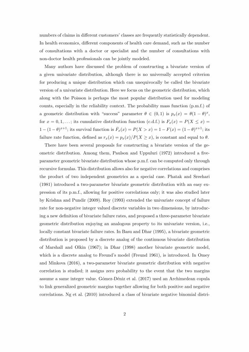
we have r(0, 0) = 1 > r(1, 1) = 0.7772 < r(2, 2) = 0.8294 (see Figure 1).
2.3. Probability Generating Function
Due to the easy analytical expression of the joint p.m.f., it is straightforward to derive
the probability generating function (p.g.f.) for the bivariate vector (X,Y ) following
the proposed bivariate geometric distribution. By definition, for a pair of r.v.s X and
5
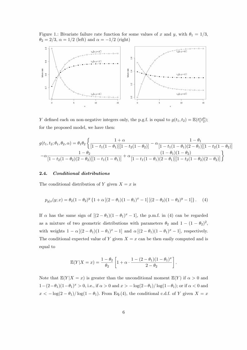
Figure 1.: Bivariate failure rate function for some values of x and y, with θ1 = 1/3,θ2 = 2/3, α = 1/2 (left) and α = −1/2 (right)
0 5 10 15
0.7
0.8
0.9
1.0
x
failu
re r
ate
rxy(x, y = 2)
rxy(x, y = 1)
rxy(x, y = 0)
0 5 10 15
1.0
1.2
1.4
1.6
x
failu
re r
ate
rxy(x, y = 2)
rxy(x, y = 1)
rxy(x, y = 0)
Y defined each on non-negative integers only, the p.g.f. is equal to g(t1, t2) = E(tx1ty2);
for the proposed model, we have then:
g(t1, t2; θ1, θ2, α) = θ1θ2
{1 + α
[1− t1(1− θ1)][1− t2(1− θ2)]− α 1− θ1
[1− t1(1− θ1)(2− θ1)][1− t2(1− θ2)]
−α 1− θ2
[1− t2(1− θ2)(2− θ2)][1− t1(1− θ1)]+ α
(1− θ1)(1− θ2)
[1− t1(1− θ1)(2− θ1)][1− t2(1− θ2)(2− θ2)]
}
2.4. Conditional distributions
The conditional distribution of Y given X = x is
py|x(y;x) = θ2(1− θ2)y {1 + α [(2− θ1)(1− θ1)x − 1] [(2− θ2)(1− θ2)y − 1]} . (4)
If α has the same sign of [(2− θ1)(1− θ1)x − 1], the p.m.f. in (4) can be regarded
as a mixture of two geometric distributions with parameters θ2 and 1 − (1 − θ2)2,
with weights 1 − α [(2− θ1)(1− θ1)x − 1] and α [(2− θ1)(1− θ1)x − 1], respectively.
The conditional expected value of Y given X = x can be then easily computed and is
equal to
E(Y |X = x) =1− θ2
θ2
[1 + α · 1− (2− θ1)(1− θ1)x
2− θ2
].
Note that E(Y |X = x) is greater than the unconditional moment E(Y ) if α > 0 and
1−(2−θ1)(1−θ1)x > 0, i.e., if α > 0 and x > − log(2−θ1)/ log(1−θ1); or if α < 0 and
x < − log(2 − θ1)/ log(1 − θ1). From Eq.(4), the conditional c.d.f. of Y given X = x
6
can be easily derived and written as:
P (Y ≤ y|X = x) = Fy(y) + αFy(y)[1− Fy(y)][1− px(x)− 2Fx(x− 1)] (5)
Symmetrical results hold for the conditional distribution and expected value of X
given Y = y.
2.5. Simulation
In order to simulate a sample from the bivariate geometric distribution with param-
eters θ1, θ2, and α, one can resort to the algorithm described in Barbiero (2017a),
properly adapted to the geometrically distributed margins with parameters θ1 and θ2.
The algorithm is based on the conditional c.d.f. in (5). The steps to be implemented
are the following:
(1) Simulate a random pair (v1, v2) from two independent uniform r.v.s in (0, 1),
V1 ∼ Unif(0, 1) and V2 ∼ Unif(0, 1);
(2) Set u = v1 and x = F−1x (u), where F−1
x denotes the quantile functions of ge-
ometric distribution with parameters θ1, i.e., x =
⌈ln(1− u)
ln(1− θ1)− 1
⌉, with d·e
indicating the ceiling function.
(3) Set v = 2v2/(a + b), where a = 1 + α(1 − px(x) − 2Fx(x − 1)) and b =[a2 − 4(a− 1)v2
]1/2. Set y =
⌈ln(1− v)
ln(1− θ2)− 1
⌉.
(4) (x, y) is a random pair from the proposed bivariate distribution.
2.6. Attainable correlations
Pearson’s correlation coefficient ρxy between the two margins can be easily calculated.
In fact, since for a geometric distribution with parameter θ1 the expected value is
equal to (1 − θ1)/θ1 and the variance is equal to (1 − θ1)/θ21, for the mixed moment
E(XY ) the following expression can be derived after some calculations:
E(XY ) =1− θ1
θ1
1− θ2
θ2+ α · 1− θ1
θ1(2− θ1)· 1− θ2
θ2(2− θ2)
and then
ρxy = α ·√
1− θ1
2− θ1·√
1− θ2
2− θ2.
7
If α = 0, X and Y are clearly uncorrelated and independent (the joint p.m.f. (2)
factorizes into the product of two univariate geometric p.m.f.s); if α > 0, we have
positively correlated marginal distributions, conversely, if α < 0, we have nega-
tively correlated marginal distributions. Since the parameter α is constrained in
[−1,min {1/(1− θ1), 1/(1− θ2)}], its range is
−√
(1− θ1)(1− θ2)
(2− θ1)(2− θ2)≤ ρxy ≤ min {1/(1− θ1), 1/(1− θ2)}
√(1− θ1)(1− θ2)
(2− θ1)(2− θ2)
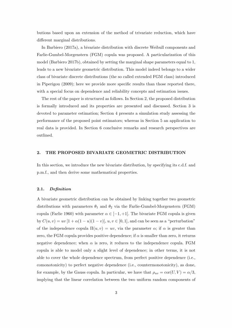
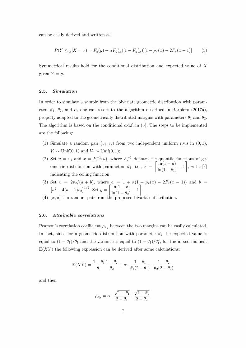
and we can observe that ρxy can never be smaller than−1/4. For identically distributed
margins with common parameter θ, the lower bound for ρxy is ρmin = −(1−θ)/(2−θ)2,
whereas the upper bound ρmax = 1/(2−θ)2 (see also Figure 2). Although the proposed
model can then yield positive as well as negative correlations, however their range is
not the largest attainable and strongly depends on the marginal parameters; this
may pose some limits on its application. In fact, we remark that for two identically
distributed geometric margins with common parameter θ, the maximum attainable
linear correlation is 1, which is achieved by linking them through the comonotonicity
copula M(u, v) = min {u, v}, whereas the minimum attainable correlation is equal to
θ − 1, if θ ≥ 1/2, whereas for θ < 1/2 it is smaller than −1/2 and can be numerically
computed by resorting to the algorithm provided in Huber and Maric (2014).
Figure 2.: Bounds of Pearson’s correlation between the margins (here supposed iden-tically distributed with common parameter θ) of the bivariate geometric model
0.0 0.2 0.4 0.6 0.8 1.0
−0.2
0.0
0.2
0.4
0.6
0.8
1.0
θ
−0.25
0.25
ρmax
ρmin
8
2.7. Reliability parameter
The probability R = P (X ≤ Y ) has been often investigated in the literature. If Y is the
strength of a component or system which is subject to a stress X, and if the system
regularly operates unless the stress exceeds the strength, then R is the probability
that the system works, i.e. a measure of system performance. The majority of pa-
pers studying the computation and estimation of R deal with independent continuous
probability distributions. However, in some real life situations, stress or strength can
have discrete distribution. For example, when the stress is the number of the products
that customers want to buy and the strength is the number of the products that fac-
tory produces (Jovanovic 2017). Furthermore, X and Y may be non-independent; this
may happen because a system that has to resist to higher levels of stress is designed to
have higher level of strength (thus implying a positive dependence/correlation between
stress and strength).
For the proposed bivariate geometric distribution, the stress-strength parameter
R = P (X ≤ Y ) can be computed as R = P (X ≤ Y ) =∑∞
y=0
∑yx=0 p(x, y) with
p(x, y) given by Eq.(2), and has the following expression:
R =θ1
1− (1− θ1)(1− θ2)+ αθ1θ2
{(2− θ1) · (2− θ2)
[1− (1− θ2)2] [1− (1− θ1)2 · (1− θ2)2]+
− (2− θ1)
θ2 [1− (1− θ1)2 · (1− θ2)]− (2− θ2)
[1− (1− θ2)2] [1− (1− θ1) · (1− θ2)2]
+1
θ2 [1− (1− θ1) · (1− θ2)]
}, (6)
which boils down to the expression reported in Maiti (1995) for the independence case
θ = 0 – there, however, the parameters θ1 and θ2 represent the complements to 1 of the
success probabilities of the two marginal geometric distributions. If we let θ1 = θ2 = θ,
i.e., if we consider two identically distributed geometric margins, then the expression
of R in (6) becomes:
R =1
2− θ+ αθ2
{(2− θ)
θ[1− (1− θ)4]− 2− θθ[1− (1− θ)3]
− 1
θ[1− (1− θ)3]+
1
θ2(2− θ)
}=
1
2− θ+ α
θ(1− θ)2
(θ2 − 2θ + 2)(θ2 − 3θ + 3)(2− θ),
which shows that R is an increasing linear function of α, once θ is fixed. For example,
if θ1 = θ2 = 0.5, then R = 2/3 in case of independence (α = 0), whereas we would have
9

Rmax = 0.7429 and Rmin = 0.6286 if α = αmax = 2 and α = αmin = −1, respectively.
The range of R looks quite short (0.1143); this is a direct consequence of the already
mentioned fact that FGM copula does not interpolate between perfect negative and
perfect positive dependence. It can be shown that the maximum value of the difference
Rmax −Rmin (≈ 0.1388) is obtained for θ ≈ 0.6858; its minimum value, 0, is obtained
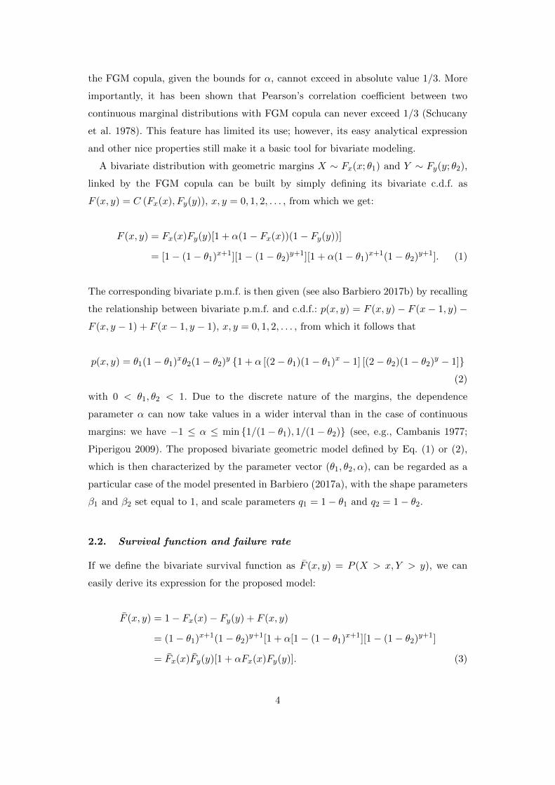
letting θ go to the boundary values 0 and 1, see Figure 3.
Figure 3.: Stress-strength parameter R for the bivariate geometric model with identicaldistributed margins with parameter θ. The two solid lines correspond to the valuesα = −1 (lower curve) and α = 1/(1− θ) (upper curve) and represent lower and upperbounds for R at a given value θ; the dashed line corresponds to the values of R whenα = 0.
0.0 0.2 0.4 0.6 0.8 1.0
0.5
0.6
0.7
0.8
0.9
1.0
θ
R
2.8. Convolution
It may be interesting to compute the distribution of the sum S = X + Y of the two
random components of the bivariate geometric distribution. Its p.m.f. can be calculated
as
ps(s) = P (S = s) =
s∑x=0
P (X = x, Y = s− x) =
=
s∑x=0
θ1(1− θ1)xθ2(1− θ2)s−x{
1 + α [(2− θ1)(1− θ1)x − 1][(2− θ2)(1− θ2)s−x − 1
]}(7)
10

If θ1 6= θ2, the expression of the p.m.f. of S becomes:
ps(s) = θ1θ2
[(1− θ2)s+1 − (1− θ1)s+1
θ1 − θ2(1 + α) + α
(1− θ2)2(s+1) − (1− θ1)2(s+1)
(1− θ2)2 − (1− θ1)2(2− θ1)(2− θ2)
−α(1− θ2)s+1 − (1− θ1)2(s+1)
1− θ2 − (1− θ1)2(2− θ1)− α(1− θ2)2(s+1) − (1− θ1)s+1
(1− θ2)2 − (1− θ1)(2− θ2)
];
(8)
whereas if θ1 = θ2 = θ, we have:
ps(s) = θ2(1− θ)s{
(s+ 1)[1 + α+ α(2− θ)2(1− θ)s]− 2α2− θθ
[1− (1− θ)s+1]
}
The expectation of S, being the two margins geometrically distributed with param-
eters θ1 and θ2, is obviously given by E(S) = E(X) + E(Y ) = 1−θ1θ1
+ 1−θ2θ2
, whatever
the value of α is. The variance of S is given by
Var(S) = Var(X)+Var(Y )+2Cov(X,Y ) =1− θ1
θ21
+1− θ2
θ22
+2α· 1− θ1
θ1(2− θ1)· 1− θ2
θ2(2− θ2),
and thus, for fixed θ1, θ2 it increases with α. If θ1 = θ2 = θ and α = 0 (independent
and identical margins) then S is distributed as a negative binomial with parameters 2
and θ and p.m.f. P (S = s) = (s+1)θ2(1−θ)s, and then E(S) = 21−θθ , Var(S) = 21−θ
θ2 .
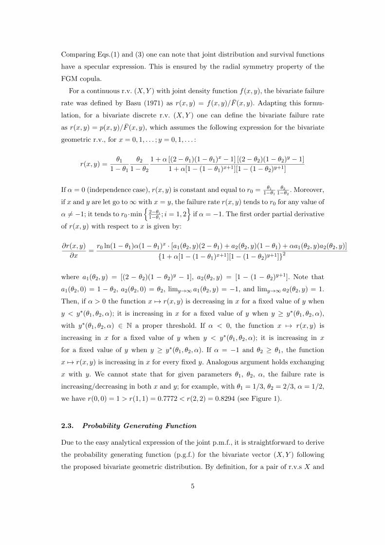
Figure 4 displays the p.m.f. of S for θ1 = θ2 = 1/3 and the three values of α, −1, 0,
3/2.
Figure 4.: P.m.f. of the sum S = X+Y for the bivariate geometric r.v. with θ1 = θ2 =1/3 and three meaningful values of α.
s
P(S
=s)
0.00
0.05
0.10
0.15
0 1 2 3 4 5 6 7 8 9 10 11 12 13 14 15
α = 3 2α = 0α = − 1
11

2.9. Regression model
The bivariate geometric distribution proposed here easily allows for the introduction
of covariates. By considering the marginal means µ1 = E(X) and µ2 = E(Y ) of the
bivariate geometric r.v., we have θt = (1 + µt)−1, t = 1, 2, and then by introducing
two vectors of covariates z and w, we can model θ1 and θ2 assuming a log-linear
relationship between marginal means and covariates:
logE(Xi|zi) = z′iβββ = zi0β0 + zi1β1 + · · ·+ zi,k−1βk−1 for i = 1, . . . , n
logE(Yi|wi) = w′iγγγ = wi0γ0 + wi1γ1 + · · ·+ wi,k−1γk−1 for i = 1, . . . , n (9)
The regression functions (9) relate the logarithm of the marginal means with the
explanatory variables; the correlation between Xi and Yi is clearly specified in terms
of the dependence parameter α. The values of the elements of βββ and γγγ, and the value
of α can be simultaneously estimated by maximizing the log-likelihood function of the
model. Among others, Famoye (2010) has already proposed an analogous regression
model for a bivariate negative binomial distribution allowing for positive, negative,
or null correlation. To simplify the analysis, one can assume that the same covariates
affect X and Y , i.e., zi = wi ∀i = 1, . . . , n.
3. ESTIMATION
Several methods for estimating the parameters θ1, θ2, and α of the proposed bivariate
distribution of Eq.(2) can be envisaged, given a random sample, (xi, yi), i = 1, 2, . . . , n.
Two versions of the method of moments are here considered as well as the standard
maximum likelihood method and a modified version thereof.
3.1. Method of Moments
A method of moments (MoM) is suggested, derived by equating the two marginal
moments with the mixed moment to the corresponding sample quantities. Denoting
with µxy = 1n
∑ni=1 xiyi the sample mixed moment, it can be easily shown that the
estimates of the marginal parameters are θ1,MoM = 1/(1 + x) and θ2,MoM = 1/(1 + y),
12
whereas for the dependence parameter α, after some algebraic passages, we have:
αMoM = (µxy − xy) · 2x+ 1
x(x+ 1)· 2y + 1
y(y + 1).
Though very easy to derive, the method of moments cannot always ensure a fea-
sible value for the estimate of α, i.e., αMoM may lie outside its natural interval
[−1,min{
1/(1− θ1,MoM ), 1/(1− θ2,MoM )}
].
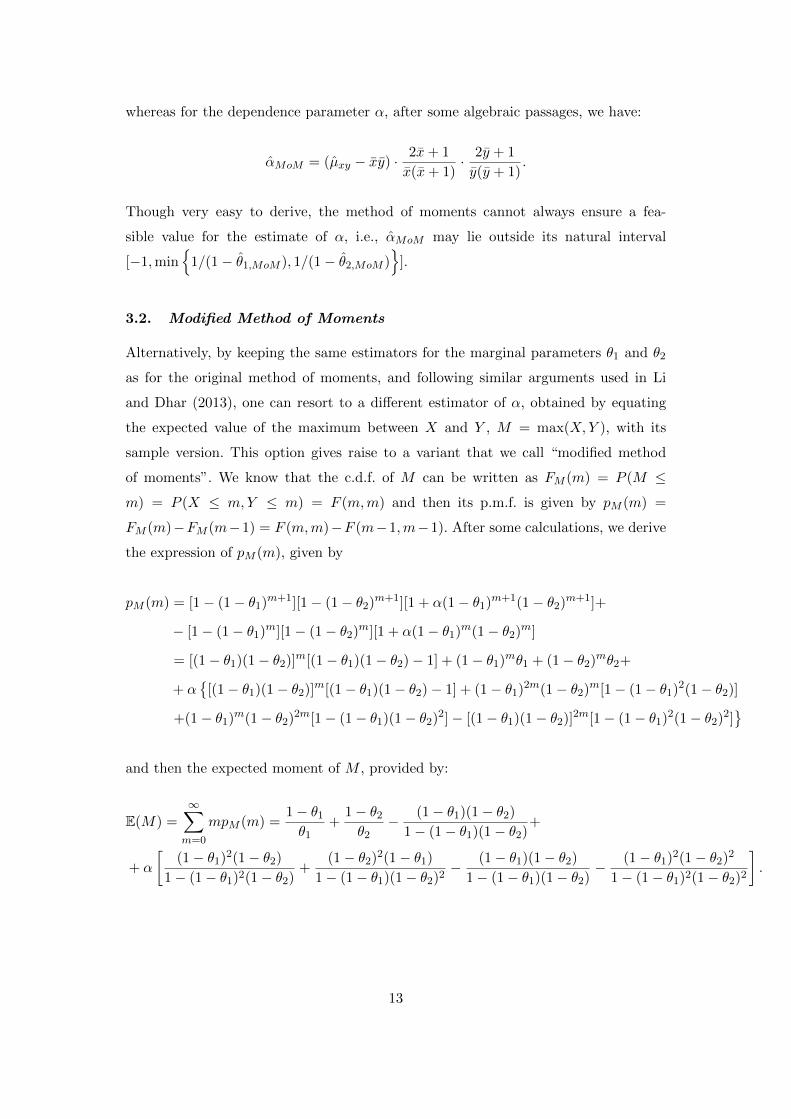
3.2. Modified Method of Moments
Alternatively, by keeping the same estimators for the marginal parameters θ1 and θ2
as for the original method of moments, and following similar arguments used in Li
and Dhar (2013), one can resort to a different estimator of α, obtained by equating
the expected value of the maximum between X and Y , M = max(X,Y ), with its
sample version. This option gives raise to a variant that we call “modified method
of moments”. We know that the c.d.f. of M can be written as FM (m) = P (M ≤
m) = P (X ≤ m,Y ≤ m) = F (m,m) and then its p.m.f. is given by pM (m) =
FM (m)−FM (m−1) = F (m,m)−F (m−1,m−1). After some calculations, we derive
the expression of pM (m), given by
pM (m) = [1− (1− θ1)m+1][1− (1− θ2)m+1][1 + α(1− θ1)m+1(1− θ2)m+1]+
− [1− (1− θ1)m][1− (1− θ2)m][1 + α(1− θ1)m(1− θ2)m]
= [(1− θ1)(1− θ2)]m[(1− θ1)(1− θ2)− 1] + (1− θ1)mθ1 + (1− θ2)mθ2+
+ α{
[(1− θ1)(1− θ2)]m[(1− θ1)(1− θ2)− 1] + (1− θ1)2m(1− θ2)m[1− (1− θ1)2(1− θ2)]
+(1− θ1)m(1− θ2)2m[1− (1− θ1)(1− θ2)2]− [(1− θ1)(1− θ2)]2m[1− (1− θ1)2(1− θ2)2]}
and then the expected moment of M , provided by:
E(M) =
∞∑m=0
mpM (m) =1− θ1
θ1+
1− θ2
θ2− (1− θ1)(1− θ2)
1− (1− θ1)(1− θ2)+
+ α
[(1− θ1)2(1− θ2)
1− (1− θ1)2(1− θ2)+
(1− θ2)2(1− θ1)
1− (1− θ1)(1− θ2)2− (1− θ1)(1− θ2)
1− (1− θ1)(1− θ2)− (1− θ1)2(1− θ2)2
1− (1− θ1)2(1− θ2)2
].
13
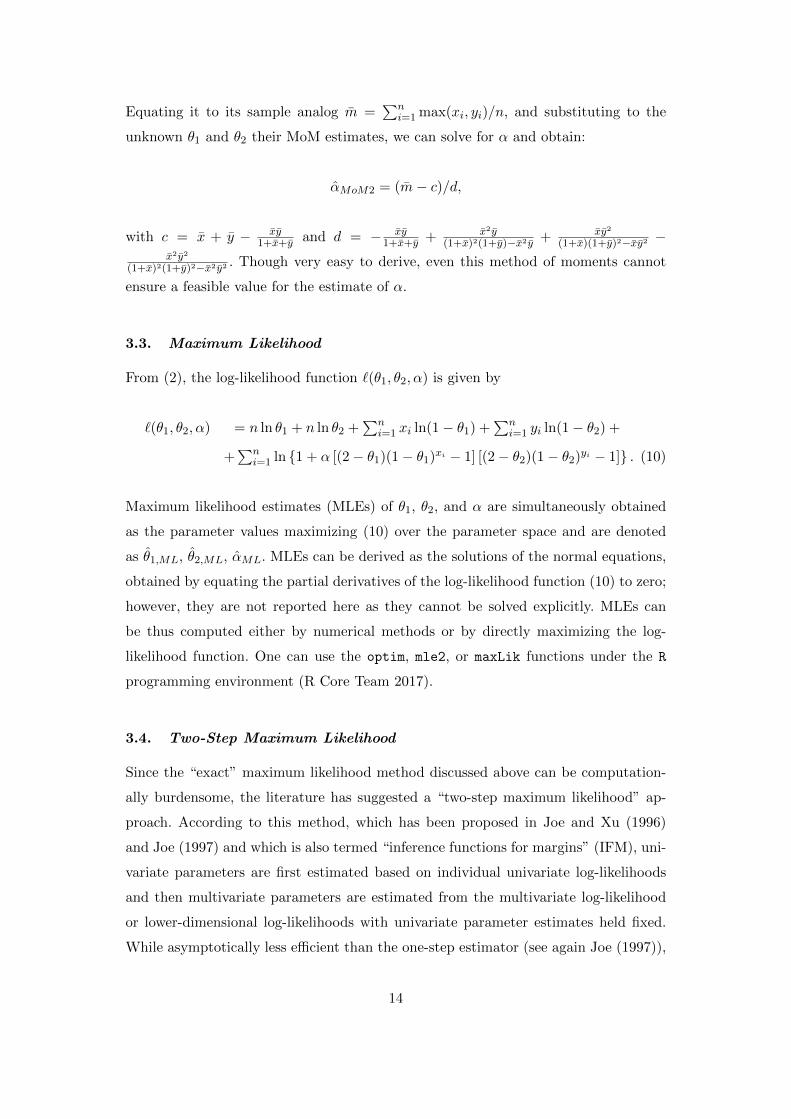
Equating it to its sample analog m =∑n
i=1 max(xi, yi)/n, and substituting to the
unknown θ1 and θ2 their MoM estimates, we can solve for α and obtain:
αMoM2 = (m− c)/d,
with c = x + y − xy1+x+y and d = − xy
1+x+y + x2y(1+x)2(1+y)−x2y + xy2
(1+x)(1+y)2−xy2 −x2y2
(1+x)2(1+y)2−x2y2 . Though very easy to derive, even this method of moments cannot
ensure a feasible value for the estimate of α.
3.3. Maximum Likelihood
From (2), the log-likelihood function `(θ1, θ2, α) is given by
`(θ1, θ2, α) = n ln θ1 + n ln θ2 +∑n
i=1 xi ln(1− θ1) +∑n
i=1 yi ln(1− θ2) +
+∑n
i=1 ln {1 + α [(2− θ1)(1− θ1)xi − 1] [(2− θ2)(1− θ2)yi − 1]} . (10)
Maximum likelihood estimates (MLEs) of θ1, θ2, and α are simultaneously obtained
as the parameter values maximizing (10) over the parameter space and are denoted
as θ1,ML, θ2,ML, αML. MLEs can be derived as the solutions of the normal equations,
obtained by equating the partial derivatives of the log-likelihood function (10) to zero;
however, they are not reported here as they cannot be solved explicitly. MLEs can
be thus computed either by numerical methods or by directly maximizing the log-
likelihood function. One can use the optim, mle2, or maxLik functions under the R
programming environment (R Core Team 2017).
3.4. Two-Step Maximum Likelihood
Since the “exact” maximum likelihood method discussed above can be computation-
ally burdensome, the literature has suggested a “two-step maximum likelihood” ap-
proach. According to this method, which has been proposed in Joe and Xu (1996)
and Joe (1997) and which is also termed “inference functions for margins” (IFM), uni-
variate parameters are first estimated based on individual univariate log-likelihoods
and then multivariate parameters are estimated from the multivariate log-likelihood
or lower-dimensional log-likelihoods with univariate parameter estimates held fixed.
While asymptotically less efficient than the one-step estimator (see again Joe (1997)),
14

this approach has the obvious advantage of reducing the dimensionality of the problem,
which is particularly useful when one has to resort to a numerical maximization. For
the bivariate distribution at study, the two-step maximum likelihood method, similarly
to the case presented in Barbiero (2017a), consists in computing first the maximum
likelihood estimates of the parameters of the two marginal geometric distributions as
if they were independent. In this case, we easily get the estimates of θ1 and θ2 as
θ1,TSML = (1 + x)−1, θ2,TSML = (1 + y)−1
(they coincide with the MoM estimates). Plugging them into the expression of the log-
likelihood (10), one can then maximize it with respect to the only remaining parameter
α (again, numerically), obtaining the estimate αTSML.
3.5. Interval estimation
Besides point estimation, asymptotic confidence intervals for each of the three param-
eters can be built based on Fisher information matrix, defined as
I(ηηη)ij = E(−∂
2 log p(x, y;ηηη)
∂ηi∂ηj
)(11)
with ηηη = (θ1, θ2, α). The second order derivatives inside Eq.(11) are cumbersome
but quite easy to compute. On the contrary, calculating their expected value is
complicated. If a bivariate sample of size n is available from the r.v. (X,Y ), one
can compute the observed Fisher Information matrix, based on the MLE of ηηη, ηηη:
I(ηηη)ij =∑n
i=1−∂2 log p(xi,yi;ηηη)
∂ηi∂ηj. Asymptotic confidence intervals can be constructed by
using the standard errors se(ηi) that can be derived by computing the inverse matrix
I(ηηη)−1. Such intervals have the usual form (ηi − z1−α/2se(ηi), ηi + z1−α/2se(ηi)), with
se(ηi) =
√[I(ηηη)−1]ii. Since the parameters ηi are bounded over a finite support, such
symmetric confidence intervals may have a poor performance in terms of coverage and
average length. For this reason, computing confidence intervals directly based on the
log-likelihood or profile log-likelihood may represent a much better choice; they often
have better small-sample properties than those based on asymptotic standard errors
computed from the full likelihood (Venzon and Moolgavkar 1988). In the statistical
environment R, the package bblmle (Bolker 2016) easily allows the user to compute
confidence intervals based on profile likelihood.
15
4. MONTE CARLO STUDY
In order to study the behaviour of the parameters’ estimators in terms of unbiased-
ness and variability, one would like to obtain their expectations and variances (or
standard errors). Finding them is almost impossible, especially for methods involving
maximum likelihood, which provide estimates in a numerical form only. Therefore,
we study numerically the expressions for expected values and standard errors with a
Monte Carlo simulation study. We consider several representative combinations of the
three parameters characterizing the proposed bivariate geometric distribution; in par-
ticular, we consider all the “distinct” combinations arising from the following choice
of parameters: θ1, θ2 = 0.25; 0.5; 0.75; α = −0.8;−0.4; 0; +0.4,+0.8,+1.2 (thus leading
to negative, null or positive dependence between the margins). “Distinct” here means
that given the symmetrical nature of the problem, if the combination corresponding
to the ordered parameter vector ηηη = (θ1, θ2, α) is considered, the combination asso-
ciated to the “symmetrical” parameter vector ηηη∗ = (θ2, θ1, α) will be skipped. This
means that 6× 6 = 36 combinations for ηηη are considered. For each of these scenarios,
the Monte Carlo simulation study is performed by generating 2, 000 samples of size
n = 100. For each sample, the four types of estimators of θ1, θ2, and α, described in
Section 3, are calculated as well as 95% confidence intervals. Then, over all the 2, 000
simulations, the means (expected values) and standard errors of these estimates are
obtained along with coverage and average length of confidence intervals. Here we will
focus on the results related to the estimates of the dependence parameter α, which are
expected to be the most meaningful, since the dependence parameter is intuitively the
most difficult to be estimated. The bivariate geometric model has been implemented
and the whole simulation study has been carried out in the R statistical environment.
Results on point estimation are reported in Tables 1 to 6. We will briefly discuss
the performance of the estimators comparatively, underlying how the dependence and
marginal parameters’ values affect it. We first remark that all four estimators are
positively biased under all the scenarios examined, except for a few scenarios with
α = 1.2; the bias magnitude is however rather small. The ML and TSML estimators
of α always have a very similar behaviour in terms of both bias and standard error
and, quite surprisingly, for positive or null values of α, TSML should be even preferred
to ML estimator, since it shows a smaller bias in absolute value and a smaller standard
error. Their performance is overall better than that of MoM estimator, except when α
is −0.8: in this case, both ML and TSML estimators show a very large bias in absolute
16

value, and in this sense MoM may be preferable; however, the standard errors of the
latter are always larger than those of the former and a significant proportion of MoM
estimates are unfeasible (smaller than−1). MoM2 estimator is overall more biased than
MoM, even if sometimes (namely, for α = 0.4; 0.8; 1.2) it presents a smaller variability.
In more detail, letting α fixed and varying the marginal parameters θ1 and θ2, one can
note that the behaviour of the four estimators (especially in terms of standard error
and to a larger extent for ML and TSML) deteriorates moving towards large values;
in particular, the scenarios characterized by θ1 = θ2 = 0.75 are the worst ones. This is
quite reasonable, since in this case the sample marginal distributions are concentrated
on the first integer numbers, with an average proportion of zeros equal to 75% for
both margins, and estimates of α are thus characterized by a large uncertainty. For a
fixed pair of values (θ1, θ2), the behavior of the standard errors of the four estimators
as a function of α is much more difficult to depict. For example, focusing on the ML
estimator, if (θ1, θ2) = (0.25, 0.25), its standard error decrease with the absolute value
of α; if (θ1, θ2) = (0.75, 0.75), the standard error is an increasing function of α.
Table 1.: Monte Carlo simulation study: mean and standard error of the estimates ofα when α = 1.2
θ1 = 0.25 θ1 = 0.5 θ1 = 0.75mean se mean se mean se
θ 1=
0.25 ML 1.193 0.203 1.186 0.234 1.173 0.268
TSML 1.184 0.215 1.180 0.234 1.169 0.268MoM 1.197 0.425 1.198 0.450 1.203 0.550
MoM2 1.226 0.397 1.225 0.379 1.222 0.378
θ 1=
0.5 ML 1.217 0.334 1.221 0.428
TSML 1.203 0.333 1.215 0.426MoM 1.201 0.484 1.209 0.594
MoM2 1.229 0.431 1.235 0.485
θ 1=
0.75 ML 1.219 0.605
TSML 1.213 0.602MoM 1.217 0.748
MoM2 1.237 0.663
In figure 5, the Monte Carlo distributions of the four point estimators of α for the
bivariate geometric model are displayed, when θ1 = θ2 = 0.5 and α = 0.8. At a first
glance, one can note that the two method of moments (MoM and MoM2) yield to
estimators characterized by a larger variability with respect to the ML and TSML
competitors. In particular, due also to the presence of many “outliers” (the isolated
points beyond the whiskers of the boxplot; most of them are unfeasible values for α),
MoM, as confirmed by the results of Table 2, presents a larger variability than MoM2.
17
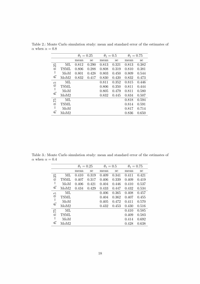
Table 2.: Monte Carlo simulation study: mean and standard error of the estimates ofα when α = 0.8
θ1 = 0.25 θ1 = 0.5 θ1 = 0.75mean se mean se mean se
θ 1=
0.25 ML 0.812 0.290 0.813 0.321 0.813 0.382
TSML 0.806 0.288 0.808 0.319 0.810 0.381MoM 0.801 0.428 0.803 0.450 0.809 0.544
MoM2 0.832 0.417 0.830 0.420 0.832 0.473
θ 1=
0.5 ML 0.811 0.352 0.815 0.446
TSML 0.806 0.350 0.811 0.444MoM 0.805 0.479 0.811 0.580
MoM2 0.832 0.445 0.834 0.507
θ 1=
0.75 ML 0.818 0.594
TSML 0.814 0.591MoM 0.817 0.714
MoM2 0.836 0.650
Table 3.: Monte Carlo simulation study: mean and standard error of the estimates ofα when α = 0.4
θ1 = 0.25 θ1 = 0.5 θ1 = 0.75mean se mean se mean se
θ 1=
0.25 ML 0.410 0.319 0.409 0.341 0.411 0.421
TSML 0.407 0.317 0.406 0.339 0.409 0.419MoM 0.406 0.421 0.404 0.446 0.410 0.537
MoM2 0.434 0.429 0.433 0.447 0.432 0.534
θ 1=
0.5 ML 0.406 0.365 0.408 0.457
TSML 0.404 0.362 0.407 0.455MoM 0.405 0.472 0.411 0.570
MoM2 0.432 0.453 0.430 0.516
θ 1=
0.75 ML 0.410 0.585
TSML 0.409 0.583MoM 0.414 0.692
MoM2 0.428 0.638
18
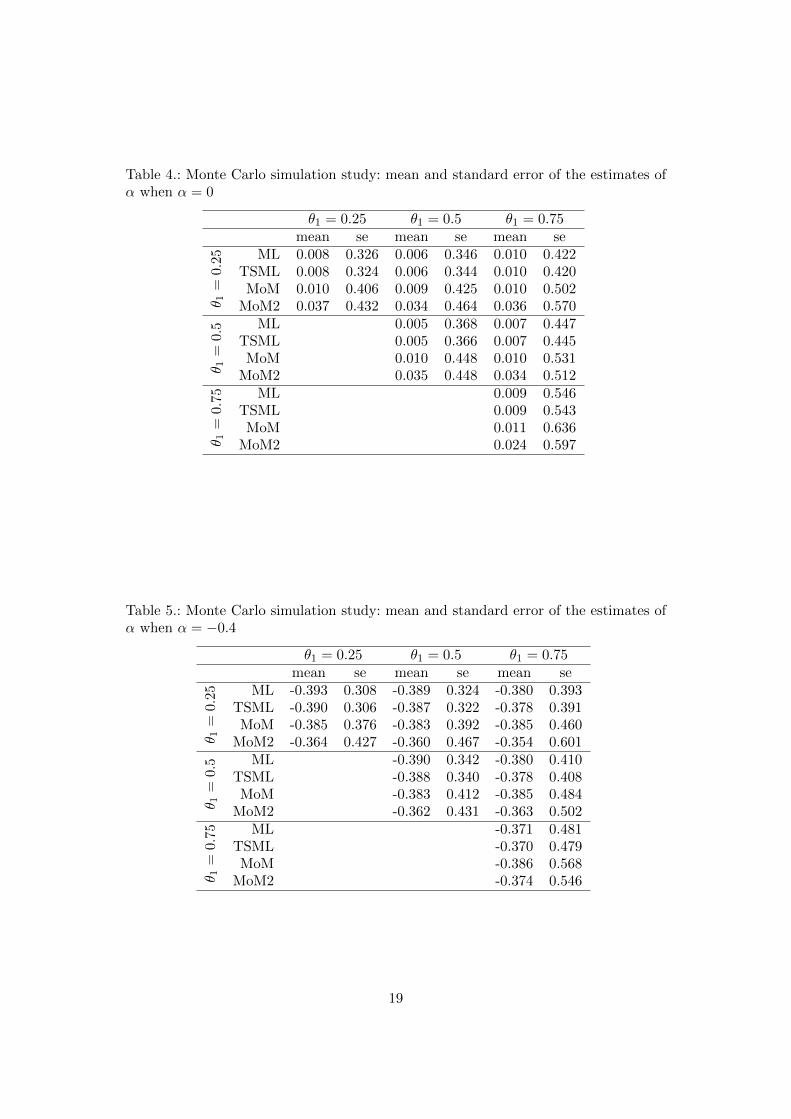
Table 4.: Monte Carlo simulation study: mean and standard error of the estimates ofα when α = 0
θ1 = 0.25 θ1 = 0.5 θ1 = 0.75mean se mean se mean se
θ 1=
0.25 ML 0.008 0.326 0.006 0.346 0.010 0.422
TSML 0.008 0.324 0.006 0.344 0.010 0.420MoM 0.010 0.406 0.009 0.425 0.010 0.502
MoM2 0.037 0.432 0.034 0.464 0.036 0.570
θ 1=
0.5 ML 0.005 0.368 0.007 0.447
TSML 0.005 0.366 0.007 0.445MoM 0.010 0.448 0.010 0.531
MoM2 0.035 0.448 0.034 0.512
θ 1=
0.75 ML 0.009 0.546
TSML 0.009 0.543MoM 0.011 0.636
MoM2 0.024 0.597
Table 5.: Monte Carlo simulation study: mean and standard error of the estimates ofα when α = −0.4
θ1 = 0.25 θ1 = 0.5 θ1 = 0.75mean se mean se mean se
θ 1=
0.25 ML -0.393 0.308 -0.389 0.324 -0.380 0.393
TSML -0.390 0.306 -0.387 0.322 -0.378 0.391MoM -0.385 0.376 -0.383 0.392 -0.385 0.460
MoM2 -0.364 0.427 -0.360 0.467 -0.354 0.601
θ 1=
0.5 ML -0.390 0.342 -0.380 0.410
TSML -0.388 0.340 -0.378 0.408MoM -0.383 0.412 -0.385 0.484
MoM2 -0.362 0.431 -0.363 0.502
θ 1=
0.75 ML -0.371 0.481
TSML -0.370 0.479MoM -0.386 0.568
MoM2 -0.374 0.546
19
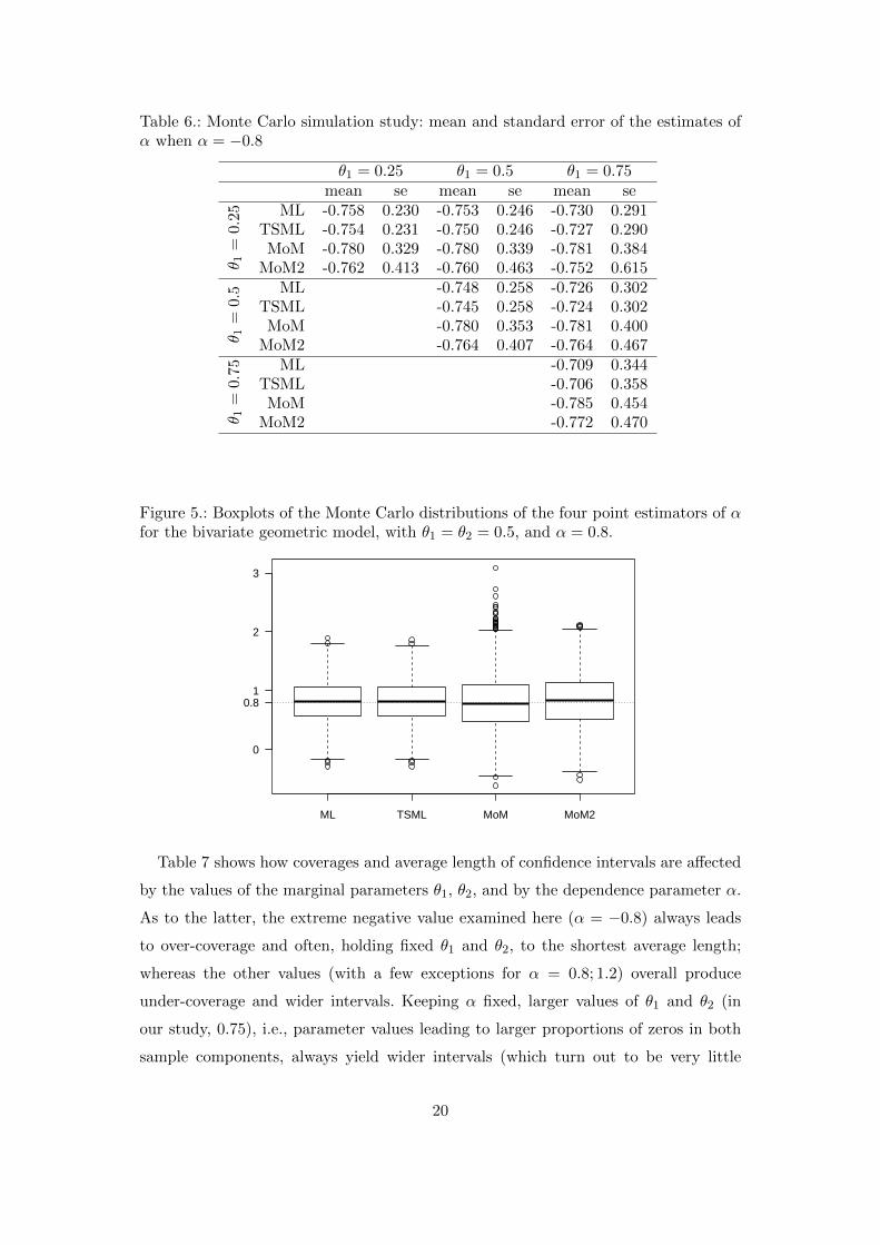
Table 6.: Monte Carlo simulation study: mean and standard error of the estimates ofα when α = −0.8
θ1 = 0.25 θ1 = 0.5 θ1 = 0.75mean se mean se mean se
θ 1=
0.25 ML -0.758 0.230 -0.753 0.246 -0.730 0.291
TSML -0.754 0.231 -0.750 0.246 -0.727 0.290MoM -0.780 0.329 -0.780 0.339 -0.781 0.384
MoM2 -0.762 0.413 -0.760 0.463 -0.752 0.615
θ 1=
0.5 ML -0.748 0.258 -0.726 0.302
TSML -0.745 0.258 -0.724 0.302MoM -0.780 0.353 -0.781 0.400
MoM2 -0.764 0.407 -0.764 0.467
θ 1=
0.75 ML -0.709 0.344
TSML -0.706 0.358MoM -0.785 0.454
MoM2 -0.772 0.470
Figure 5.: Boxplots of the Monte Carlo distributions of the four point estimators of αfor the bivariate geometric model, with θ1 = θ2 = 0.5, and α = 0.8.
ML TSML MoM MoM2
0
1
2
3
0.8
Table 7 shows how coverages and average length of confidence intervals are affected
by the values of the marginal parameters θ1, θ2, and by the dependence parameter α.
As to the latter, the extreme negative value examined here (α = −0.8) always leads
to over-coverage and often, holding fixed θ1 and θ2, to the shortest average length;
whereas the other values (with a few exceptions for α = 0.8; 1.2) overall produce
under-coverage and wider intervals. Keeping α fixed, larger values of θ1 and θ2 (in
our study, 0.75), i.e., parameter values leading to larger proportions of zeros in both
sample components, always yield wider intervals (which turn out to be very little
20
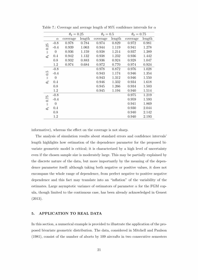
Table 7.: Coverage and average length of 95% confidence intervals for α
θ2 = 0.25 θ2 = 0.5 θ2 = 0.75α coverage length coverage length coverage length
θ 1=
0.25
-0.8 0.978 0.784 0.974 0.829 0.972 0.981-0.4 0.939 1.063 0.944 1.119 0.941 1.278
0 0.936 1.159 0.938 1.214 0.937 1.3890.4 0.942 1.132 0.938 1.232 0.936 1.4420.8 0.932 0.883 0.936 0.924 0.928 1.0471.2 0.974 0.684 0.972 0.770 0.974 0.924
θ 1=
0.5
-0.8 0.978 0.872 0.976 1.028-0.4 0.943 1.174 0.946 1.354
0 0.943 1.312 0.946 1.5500.4 0.946 1.332 0.934 1.6180.8 0.945 1.266 0.934 1.5031.2 0.945 1.194 0.940 1.514
θ 1=
0.75
-0.8 0.975 1.219-0.4 0.959 1.593
0 0.941 1.8690.4 0.930 2.0440.8 0.940 2.1421.2 0.940 2.193
informative), whereas the effect on the coverage is not sharp.
The analysis of simulation results about standard errors and confidence intervals’
length highlights how estimation of the dependence parameter for the proposed bi-
variate geometric model is critical; it is characterized by a high level of uncertainty
even if the chosen sample size is moderately large. This may be partially explained by
the discrete nature of the data, but more importantly by the meaning of the depen-
dence parameter itself: although taking both negative or positive values, it does not
encompass the whole range of dependence, from perfect negative to positive negative
dependence and this fact may translate into an “inflation” of the variability of the
estimates. Large asymptotic variance of estimators of parameter α for the FGM cop-
ula, though limited to the continuous case, has been already acknowledged in Genest
(2013).
5. APPLICATION TO REAL DATA
In this section, a numerical example is provided to illustrate the application of the pro-
posed bivariate geometric distribution. The data, considered in Mitchell and Paulson
(1981), consist of the number of aborts by 109 aircrafts in two consecutive semesters
21
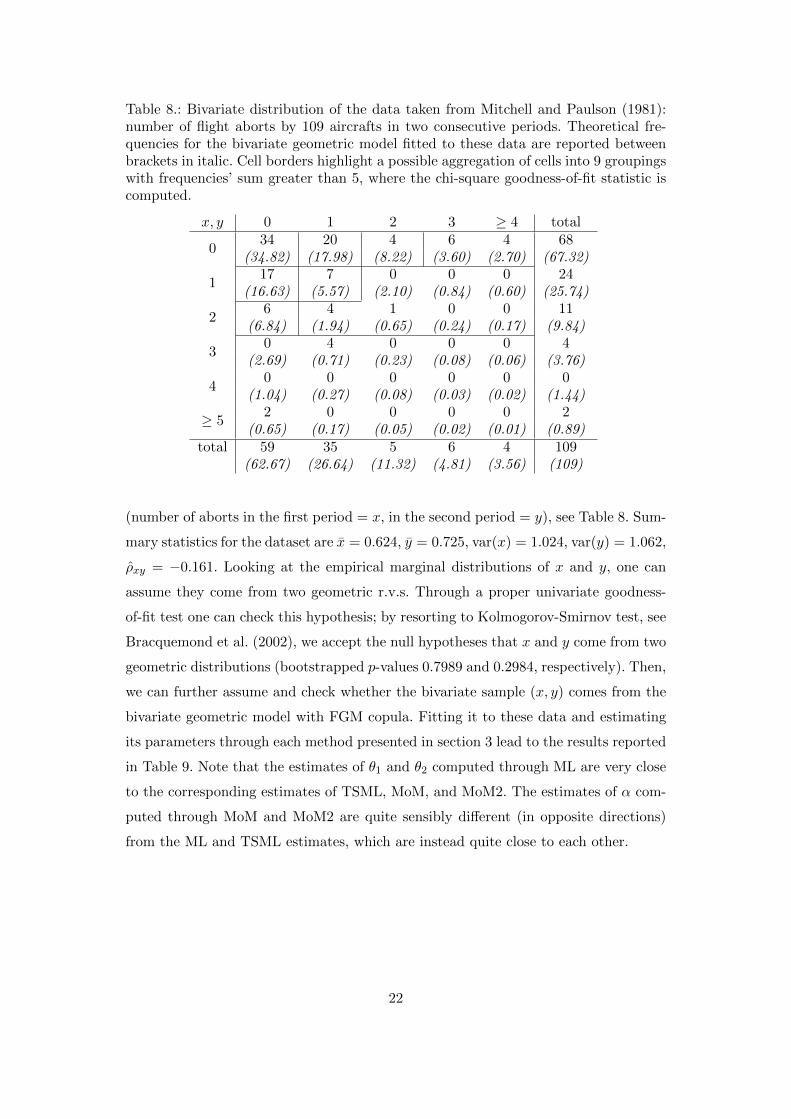
Table 8.: Bivariate distribution of the data taken from Mitchell and Paulson (1981):number of flight aborts by 109 aircrafts in two consecutive periods. Theoretical fre-quencies for the bivariate geometric model fitted to these data are reported betweenbrackets in italic. Cell borders highlight a possible aggregation of cells into 9 groupingswith frequencies’ sum greater than 5, where the chi-square goodness-of-fit statistic iscomputed.
x, y 0 1 2 3 ≥ 4 total
034 20 4 6 4 68
(34.82) (17.98) (8.22) (3.60) (2.70) (67.32)
117 7 0 0 0 24
(16.63) (5.57) (2.10) (0.84) (0.60) (25.74)
26 4 1 0 0 11
(6.84) (1.94) (0.65) (0.24) (0.17) (9.84)
30 4 0 0 0 4
(2.69) (0.71) (0.23) (0.08) (0.06) (3.76)
40 0 0 0 0 0
(1.04) (0.27) (0.08) (0.03) (0.02) (1.44)
≥ 52 0 0 0 0 2
(0.65) (0.17) (0.05) (0.02) (0.01) (0.89)total 59 35 5 6 4 109
(62.67) (26.64) (11.32) (4.81) (3.56) (109)
(number of aborts in the first period = x, in the second period = y), see Table 8. Sum-
mary statistics for the dataset are x = 0.624, y = 0.725, var(x) = 1.024, var(y) = 1.062,
ρxy = −0.161. Looking at the empirical marginal distributions of x and y, one can
assume they come from two geometric r.v.s. Through a proper univariate goodness-
of-fit test one can check this hypothesis; by resorting to Kolmogorov-Smirnov test, see
Bracquemond et al. (2002), we accept the null hypotheses that x and y come from two
geometric distributions (bootstrapped p-values 0.7989 and 0.2984, respectively). Then,
we can further assume and check whether the bivariate sample (x, y) comes from the
bivariate geometric model with FGM copula. Fitting it to these data and estimating
its parameters through each method presented in section 3 lead to the results reported
in Table 9. Note that the estimates of θ1 and θ2 computed through ML are very close
to the corresponding estimates of TSML, MoM, and MoM2. The estimates of α com-
puted through MoM and MoM2 are quite sensibly different (in opposite directions)
from the ML and TSML estimates, which are instead quite close to each other.
22

Table 9.: Parameter estimates for the bivariate geometric model applied to Mitchelland Paulson (1981) data.
method θ1 θ2 αML 0.6176 0.5749 -0.6174
TSML 0.6158 0.5798 -0.6091MoM 0.6158 0.5798 -0.7293MoM2 0.6158 0.5798 -0.4548
The observed Fisher Information Matrix is given by:
I(ηηη) =
0.001341 −0.000183 −0.000737
−0.000183 0.001313 0.002217
−0.000737 0.002217 0.158698
from which the asymptotic standard errors of the three MLEs can be easily derived:
se(θ1) = 0.036618, se(θ2) = 0.036238, se(α) = 0.398370. Note the large uncertainty
associated to the dependence parameter α. 95% confidence intervals for the three
parameters based on profile log-likelihood are provided as (θ1L, θ1U ) = (0.5445, 0.6873),
(θ2L, θ2U ) = (0.5034, 0.6446), (α1L, α1U ) = (−1, 0.1730).
The value of the log-likelihood function computed at the MLEs is `max = −244.63
and the corresponding value of the Akaike Information Criterion (AIC = 2k − 2`max,
with k = 3 being the number of parameters) is 495.26. The bivariate negative binomial
distribution proposed in Mitchell and Paulson (1981) showed an AIC equal to 498.54,
thus indicating a worse fit to the data; the bivariate discrete Weibull distribution
proposed in Barbiero (2017a), though obviously providing a greater value of the log-
likelihood function (−243.966), provides a greater value of the AIC (497.93), thus
denoting again a worse fit than the proposed bivariate geometric model. The bivariate
geometric distribution proposed by Roy (1993) yields a better fit: the AIC is equal to
494.0382, being the maximum value of the log-likelihood function −244.0191. In order
to obtain an “absolute” measure of fit of the proposed bivariate model, we can resort
to the standard chi-square goodness-of-fit test. We computed the theoretical absolute
joint frequencies, by using the p.m.f. in (2) with the MLEs of the parameters θ1, θ2
and α; they are displayed between brackets in Table 8. Then we aggregated cells in
order to obtain for each grouping an aggregate frequency larger than 5; we computed
the chi-square statistic as χ2 =∑G
g=1(ng − ng)2/ng, where ng is the observed count
for grouping g, ng is its theoretical analog, G is the number of groupings (in this case
23
G = 9). Under the null hypothesis that the bivariate sample comes from the proposed
distribution, χ2 is approximately distributed as a chi-square r.v. with 9 − 3 − 1 = 5
degrees of freedom. The empirical value of χ2 is 5.434; its p-value is 0.365 and being
far larger than 0 it denotes a satisfactory fit of the model to the data.
Plugging in the MLEs of the three parameters into (6), one derives the MLE of
R as R = 0.7123997, which represents the estimated probability that the number of
aborts in the second period is not smaller than the number of aborts in the first one.
By the way, the MLE of R is very close to the standard non-parametric estimate
R = 1n
∑ni=1 1xi≤yi = 76/109 = 0.6972477.
6. CONCLUSION
The bivariate geometric model proposed in this work is able to handle correlated ge-
ometrically distributed counts with a moderate level of dependence, regulated by the
unique parameter of the Farlie-Gumbel-Morgenstern (FGM) copula linking its uni-
variate margins. It can be employed in several fields where discrete data arise, such
as industrial quality control, insurance, health economics, marketing, an so on. The
easy form of the joint probability mass function allows to derive interesting analytical
results for the bivariate failure rate, attainable correlations, conditional distributions
and moments, reliability parameter, and, partially, estimation. Moreover, the parame-
ter components have a clear interpretation. An application to a real dataset, reporting
the number of failures occurred to a group of aircrafts in two consecutive periods,
has shown how the model can be easily fitted. However, we are aware that the use
of this bivariate discrete model may lead to some problems when modeling real data
(the natural space of the dependence parameter depends on the values of the marginal
parameters; the model can allow only for a moderate linear correlation, whose lower
and upper bounds depend again on the values of the marginal parameters) and in the
estimation step (even for moderately large sample size, estimators of the dependence
parameter can be little precise). Further research will investigate possible extensions
of the model accommodating a wider range of dependence, by resorting to generalized
FGM copulas, and thus possibly tackling also drawbacks in estimation. We hope that
the proposed model will be a viable alternative to the existing models dealing with
the kind of data sets considered here.
24
Aknowledgments
I would like to thank the Editor and two anonymous reviewers for their constructive
comments, which helped me to improve the final version of the paper.
References
Barbiero, A.: Discrete Weibull variables linked by Farlie-Gumbel-Morgenstern copula. In AIP
Conference Proceedings 1863(240006). AIP Publishing (2017a).
Barbiero, A.: A bivariate geometric distribution with positive or negative correlation. In AIP
Conference Proceedings 1906(110003). AIP Publishing (2017b).
Basu, A. P.: Bivariate failure rate. J. Amer. Statist. Assoc. 66(333), 103-104 (1971).
Basu, A.P., Dhar, S.K.: Bivariate geometric distribution. J. Appl. Statist. Sci. 2, 33-44 (1995).
Bolker, B., R Development Core Team. bbmle: Tools for General Maximum Likelihood Esti-
mation. R package version 1.0.18 (2016). https://CRAN.R-project.org/package=bbmle
Bracquemond, C., Cretois, E., Gaudoin, O.: A comparative study of goodness-of-fit tests for
the geometric distribution and application to discrete time reliability. Laboratoire Jean
Kuntzmann, Applied Mathematics and Computer Science, Technical Report (2002).
Cambanis, S. (1977). Some properties and generalizations of multivariate Eyraud-Gumbel-
Morgenstern distributions. J. Multivariate Anal. 7(4), 551-559.
Dhar, S.K.: Data analysis with discrete analog of Freund’s model. J. Appl. Statist. Sci. 7,
169-183 (1998).
Famoye, F. (2010). On the bivariate negative binomial regression model. J. Appl. Statist.
37(6), 969-981.
Farlie, D.J.G. (1960). The performance of some correlation coefficient for a general bivariate
distribution. Biometrika 47, 307-323.
Freund, J.E. (1961). A bivariate extension of the exponential distribution. J. Amer. Statist.
Assoc. 56, 971-977.
Genest, C., Carabarın-Aguirre, A., Harvey, F. (2013). Copula parameter estimation using
Blomqvist’s beta. Journal de la Societe Francaise de Statistique, 154(1), 5-24.
Gomez-Deniz, E., Ghitany, M.F., Gupta, R.C. (2017). A bivariate generalized geometric dis-
tribution with applications, Commun. Stat. Theory Methods 46(11), 5453-5465.
Huber, M., Maric, N. (2014). Minimum correlation for any bivariate Geometric distribution.
Alea, 11(1): 459-470.
Joe, H. and Xu, J. J. (1996). The estimation method of inference functions for margins for
multivariate models. UBC, Department of Statistics, Technical Report, 166.
Joe, H. (1997). Multivariate Models and Dependence Concepts. Chapman & Hall, London.
25
Johnson, N.L., Kotz, S., Balakrishnan, N. (1997). Discrete Multivariate Distributions. Wiley,
New York.
Jovanovic, M. (2017). Estimation of P {X < Y } for Geometric-Exponential Model Based on
Complete and Censored Samples, Commun. Stat. Simul. Computat. 46(4), 3050-3066.
Kocherlakota, S. and Kocherlakota, K. (1992). Bivariate Discrete Distributions. Marcel Dekker,
New York.
Krishna, H., Pundir, P.S. (2009). A bivariate geometric distribution with applications to reli-
ability. Commun. Stat. Theory Methods 38(7), 1079-1093.
Li, J., Dhar, S.K. (2013). Modeling with Bivariate Geometric Distributions, Commun. Stat.
Theory Methods 42(2), 252-266.
Maiti, S.S. (1995). Estimation of P (X ≤ Y ) in the Geometric Case, J. Indian Statist. Assoc.
33, 87-91.
Marshall, A.W., Olkin, I. (1967). A multivariate exponential distribution. J. Amer. Statist.
Assoc. 62, 30-44.
Mitchell, C.R., Paulson, A.S. (1981). A new bivariate negative binomial distribution, Nav. Res.
Logist. Q. 28, 359-374.
Ng, C. M., Ong, S. H., Srivastava, H. M. (2010). A class of bivariate negative binomial distri-
butions with different index parameters in the marginals. Applied Math. Comput. 217(7),
3069-3087.
Omey, E., Minkova, L. D. (2013). Bivariate geometric distributions. Hub Research Papers
Economics and Business Science.
Paulson, A.S., Uppuluri, V.R.R. (1972). A characterization of the geometric distribution and
a bivariate geometric distribution. Sankhya Ser. A, 297-300.
Piperigou, V. (2009). Discrete distributions in the extended FGM family. J Statist. Plann.
Inference 139(11), 3891-3899.
Phatak, A.G., Sreehari, M. (1981). Some characterizations of a bivariate geometric distribution.
J. Indian Statist. Assoc. 19, 141-146.
R Core Team, R: A language and environment for statistical computing, R Foundation for
Statistical Computing, Vienna, Austria. URL https://www.R-project.org/ (2017).
Roy, D. (1993). Reliability measures in the discrete bivariate set-up and related characteriza-
tion results for a bivariate geometric distribution. J. Multivariate Anal. 46(2), 362-373.
Sarabia, J.M., Gomez-Deniz, E. (2011). Multivariate Poisson-Beta Distributions with Appli-
cations. Commun. Stat. Theory Methods 40(6): 1093-1108.
Schucany, W., Parr, W.C., Boyer, J.E. (1978). Correlation structure in Farlie-Gumbel-
Morgenstern distributions. Biometrika 65(3), 650-653.
Venzon, D. J., Moolgavkar, S. H. (1988). A method for computing profile-likelihood-based
confidence intervals. Applied Stat. 37(1), 87-94.
26