RISK, INFLATION, AND THE STOCK MARKET

by

Robert S. Pindyck

Massachusetts Institute of Technology

January 1983

Revised: April 1983

WP #1423-83

This research was supported by the National Science Foundationunder Grant No. SES-8012667, and that support is gratefullyacknowledged. The author also wants to thank Laurent Guy forhis research assistance, and Andrew Abel, Fischer Black, ZviBodie, Benjamin Friedman, Daniel Holland, Julio Rotemberg,Richard Ruback, Robert Shiller, and Lawrence Summers for help-ful discussions and comments.

ABSTRACT

Most explanations for the decline in share values over the past

two decades have focused on the concurrent increase in inflation.

This paper considers an alternative explanation: a substantial in-

crease in the riskiness of capital investments. We show that the

variance of the firm's real marginal return on capital has increased

significantly over the past two decades, that this has increased the

relative riskiness of investors' net real returns from holding stocks,

and that this in turn can explain a large part of the market decline.

1. Introduction

From January 1965 to December 1981 the New York Stock Exchange Index declined

by about 68 percent in real terms. Including dividends, the average real return

as measured by this index was close to zero. Most explanations of this perfor-

mance focus on the concurrent increase in the average rate of inflation. For

example, Modigliani and Cohn (1979) suggested that investors systematically con-

fuse real and nominal discount rates when valuing equity, Fama (1981) associates

higher inflation rates with changes in real variables that reduce the return on

capital, and Feldstein (1981a) argues that increased inflation reduces share

prices because of the interaction of inflation with the tax system.

Feldstein (1981a,b) and Summers (1981a,b) claim that this last effect can

explain a large fraction of the decline in share prices. The main sources of

the effect are the "historic cost" method of depreciation and the taxation of

nominal capital gains, both of which cause the net return from stock to fall when

inflation rises. However, inflation also reduces the real value of the firm's

debt, and reduces the net real return on bonds. The size and direction of the

overall effect has been debated, and it clearly depends on the values of tax and

3other parameters. I will argue that increases in expected inflation -- together

with concurrent increases in the variance of inflation -- should have had a small

and possibly positive effect on share values.

Malkiel (1979) suggested another reason for the decline in share prices:

changes occurred in the U.S. economy during the 1970's that substantially in-

creased the riskiness of capital investments.4 This paper elaborates on and

supports Malkiel's suggestion. It shows that the variance of the firm's real

gross marginal return on capital has increased significantly since 1965, that

this has increased the relative riskiness of investors' net real returns from

holding stocks, and that this in turn can explain a large fraction of the

market decline.

-2-

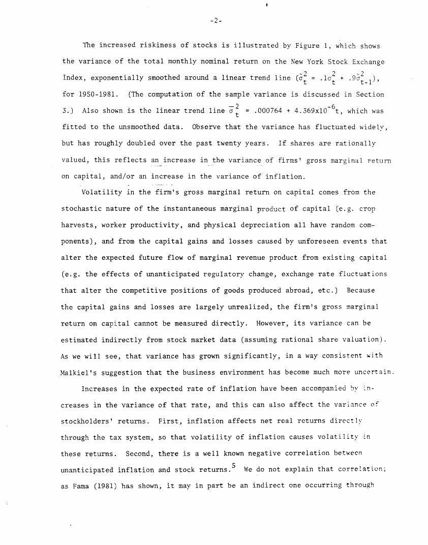
The increased riskiness of stocks is illustrated by Figure 1, which shows

the variance of the total monthly nominal return on the New York Stock Exchange

-2 2 2Index, exponentially smoothed around a linear trend line ( = .la + .9 2

for 1950-1981. (The computation of the sample variance is discussed in Section

-2 -63.) Also shown is the linear trend line at .000764 + 4.369x0 t, which was

fitted to the unsmoothed data. Observe that the variance has fluctuated widely,

but has roughly doubled over the past twenty years. If shares are rationally

valued, this reflects an increase in the variance of firms' gross marginal return

on capital, and/or an increase in the variance of inflation.

Volatility in the firm's gross marginal return on capital comes from the

stochastic nature of the instantaneous marginal product of capital (e.g. crop

harvests, worker productivity, and physical depreciation all have random com-

ponents), and from the capital gains and losses caused by unforeseen events that

alter the expected future flow of marginal revenue product from existing capital

(e.g. the effects of unanticipated regulatory change, exchange rate fluctuations

that alter the competitive positions of goods produced abroad, etc.) Because

the capital gains and losses are largely unrealized, the firm's gross marginal

return on capital cannot be measured directly. However, its variance can be

estimated indirectly from stock market data (assuming rational share valuation).

As we will see, that variance has grown significantly, in a way consistent with

Malkiel's suggestion that the business environment has become much more uncertain.

Increases in the expected rate of inflation have been accompanied by n-

creases in the variance of that rate, and this can also affect the variance of

stockholders' returns. First, inflation affects net real returns directly

through the tax system, so that volatility of inflation causes volatility in

these returns. Second, there is a well known negative correlation between

unanticipated inflation and stock returns.5 We do not explain that correlation;

as Fama (1981) has shown, it may in part be an indirect one occurring through

-3-

correlations with real economic variables. However, it implies a negative cor-

relation between unanticipated inflation and the gross marginal return on

capital, so that volatility of inflation will be associated with volatility in

that gross return.6

On the other hand, an increased volatility of inflation also increases the

riskiness of nominal bonds. The relative size of the effect again depends on

tax rates and other parameters, but we will see that overall a more volatile

inflation rate makes bonds relatively riskier, and should therefore increase

share values.

The next section of this paper shows how investors' net real returns on

equity and bonds depend on taxes, inflation, and the gross marginal return on

capital. The specification of those returns extends Feldstein's (1980b) model

so that risk is treated explicitly. In Section 3 we discuss the data and para-

meter values, estimate the variance of the gross marginal return on capital and

its covariance with inflation, and examine their behavior over time. In Section

4 a simple optimal portfolio model is used to relate changes in the price of

equity to changes in the mean and variance of inflation, and the mean and vari-

ance of the marginal return on capital. Section 5 shows how changes in these

means and variances over the past two decades can explain a good part of the

behavior of share values.

Before proceeding, the main argument of this paper can be illustrated with

two simple regressions. Summers (1981a) used a "rolling ARIMA" forecast to

generate an expected inflation series, Are(t), and then (using quarterly data

for 1958-78) regressed the real excess returns on the NYSE Index on the change

in the expected inflation, Ae(t). He obtained a negative coefficient for A e ,

supporting his argument that increases in inflation cause decreases in share

values.

I computed a similar series for e (t), using annual averages of a rolling

ARIMA forecast of monthly data.7 The corresponding OLS regression, for the

-4-

period 1958-81, is shown below (t- statistics in parentheses):

ER = .00335 - 3 .615 R2 = .193(1.19) (-2.29) SER = .0137

D.W. = 1.93

As in Summers' regression, the coefficient of e is negative and significant.

But now let us add another explanatory variable, the change in the variance of

stock returns, Aa 2s

ER = .00258 + 1.4 81AIe - 8.936A 2 R = .488(1.12) (0.76) (-3.48)s SER = .0112

D.W. = 1.85

Observe that the coefficient of A 2 is negative and highly significant, while the

coefficient of A e is now insignificantly different from zero. This simple

regression suggests that increased risk and not increased inflation caused share

values to decline. The analysis that follows explores that possibility.

2. Asset Returns

For simplicity, portfolio choice in this paper is limited to two assets,

stocks and nominal bonds. I treat the rate of inflation as stochastic, so that

the real returns on both of these assets are risky. Trading is assumed to take

place continuously and with negligible transactions costs, and asset returns

are described as continuous-time stochastic processes. As we will see, this

provides a convenient framework for analyzing the effects of risk. Inithis

section we derive and discuss expressions for investors' real after-tax asset

returns. All of the parameters and symbols introduced here and throughout the

paper are summarized in Appendix A.

A. The Return on Bonds

We describe inflation and bond returns as in Fischer (1975). The price level

follows a geometric random walk, so that the instantaneous rate of inflation is

given by

dP/P = 7dt + ldzl (1)

III

-5-

where dz = El(t)d, with el(t) a serially uncorrelated and normally distributed

random variable with zero mean and unit variance, i.e. zl(t) is a Wiener process.

Thus over an interval dt, expected inflation is rdt and its variance is adt.

Bonds are short-term, and yield a (guaranteed) gross nominal rate of return

R. We can view this return as an increase in the nominal price of a bond, i.e.

dPB/P = Rdt (2)

The gross real return on the bond is therefore:9

d(PB/P)/(PB/P) = (R - + al)dt - aldzl (3)

Interest payments are taxed as income, so the investor's net nominal return on

bonds is (l-e)Rdt, where 8 is the personal income tax rate. The net real return

on bonds over an interval dt is therefore:

Sb = [(1-e)R - + o]dt - aldzl (4)

= rbdt - oldzl

This characterization of bond returns contains the simplifying assumption

that stochastic changes in the price level are serially uncorrelated.l° If

inflation actually followed (1), the real return on long-term bonds would be

no riskier than that on short-term bonds.1 In reality stochastic changes in

the price level are autocorrelated, so that long-term bonds are indeed riskier.

Our model could be expanded by adding long-term bonds as a third asset and

allowing for autocorrelation in price changes, but the added complication would

buy little in the way of additional insight, and would not qualitatively change

any of the basic results.

B. The Return on Stocks

To derive an expression for investors' net real return on stocks, we begin

with a description of the firm's gross marginal return on capital. Following

-6-

Feldstein (1980b), we then introduce the effects of inflation and taxes.

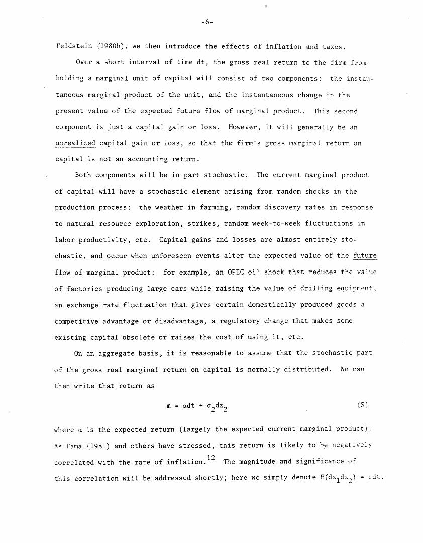
Over a short interval of time dt, the gross real return to the firm from

holding a marginal unit of capital will consist of two components: the instan-

taneous marginal product of the unit, and the instantaneous change in the

present value of the expected future flow of marginal product. This second

component is just a capital gain or loss. However, it will generally be an

unrealized capital gain or loss, so that the firm's gross marginal return on

capital is not an accounting return.

Both components will be in part stochastic. The current marginal product

of capital will have a stochastic element arising from random shocks in the

production process: the weather in farming, random discovery rates in response

to natural resource exploration, strikes, random week-to-week fluctuations in

labor productivity, etc. Capital gains and losses are almost entirely sto-

chastic, and occur when unforeseen events alter the expected value of the future

flow of marginal product: for example, an OPEC oil shock that reduces the value

of factories producing large cars while raising the value of drilling equipment,

an exchange rate fluctuation that gives certain domestically produced goods a

competitive advantage or disadvantage, a regulatory change that makes some

existing capital obsolete or raises the cost of using it, etc.

On an aggregate basis, it is reasonable to assume that the stochastic part

of the gross real marginal return on capital is normally distributed. We can

then write that return as

m = adt + a2dz2 (5

where is the expected return (largely the expected current marginal product).

As Fama (1981) and others have stressed, this return is likely to be negatively

correlated with the rate of inflation.l 2 The magnitude and significance of

this correlation will be addressed shortly; here we simply denote E(dzldz2) = pdt.

-7-

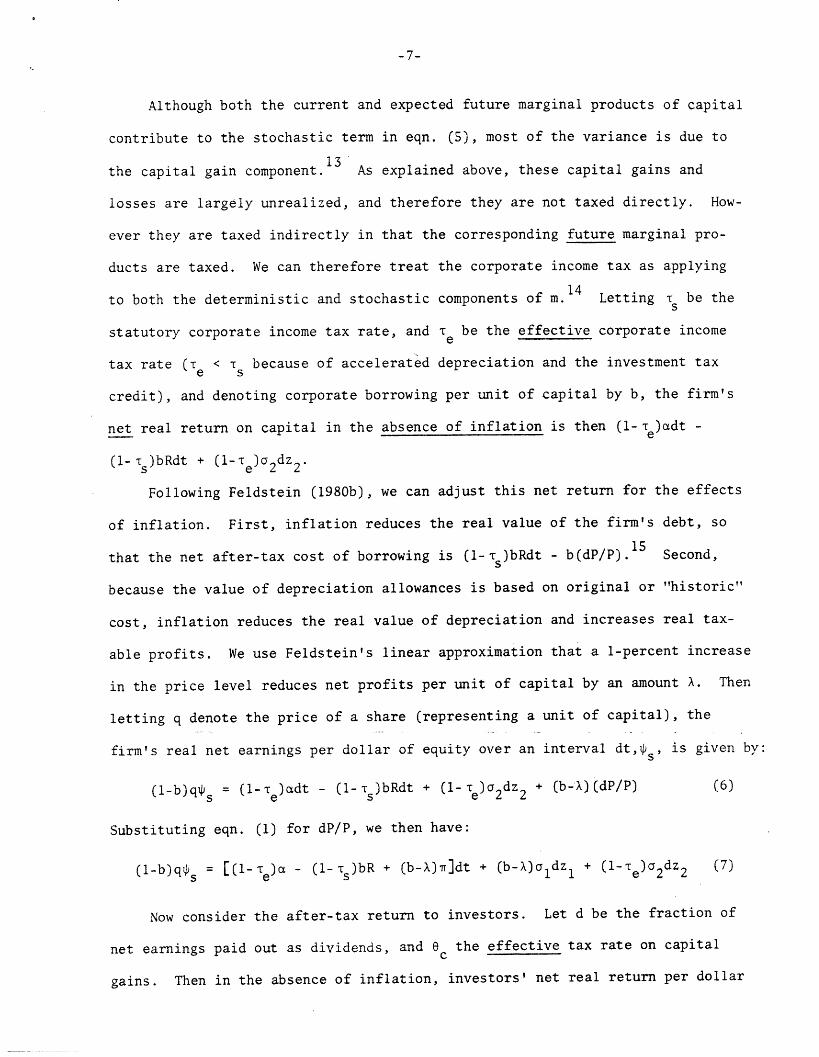
Although both the current and expected future marginal products of capital

contribute to the stochastic term in eqn. (5), most of the variance is due to

the capital gain component. As explained above, these capital gains and

losses are largely unrealized, and therefore they are not taxed directly. How-

ever they are taxed indirectly in that the corresponding future marginal pro-

ducts are taxed. We can therefore treat the corporate income tax as applying

to both the deterministic and stochastic components of m.14 Letting T be the

statutory corporate income tax rate, and Te be the effective corporate income

tax rate ( e < Ts because of accelerated depreciation and the investment tax

credit), and denoting corporate borrowing per unit of capital by b, the firm's

net real return on capital in the absence of inflation is then (1- Te)adt -

(1- s)bRdt + (1-~e)a 2dz 2 .

Following Feldstein (1980b), we can adjust this net return for the effects

of inflation. First, inflation reduces the real value of the firm's debt, so

that the net after-tax cost of borrowing is (l-sr )bRdt - b(dP/P).15 Second,

because the value of depreciation allowances is based on original or "historic"

cost, inflation reduces the real value of depreciation and increases real tax-

able profits. We use Feldstein's linear approximation that a 1-percent increase

in the price level reduces net profits per unit of capital by an amount . Then

letting q denote the price of a share (representing a unit of capital), the

firm's real net earnings per dollar of equity over an interval dt, s, is given by:

(l-b)q = (l-T)adt - (1-T )bRdt + (l-Te)a2dz2 + (b-X)(dP/P) (6)e s

Substituting eqn. (1) for dP/P, we then have:

(l-b)q s = [(l-Te)a - (l- s)bR + (b-X)]dt + (b-X)aldz1 + (l-re)a2dz2 (7)

Now consider the after-tax return to investors. Let d be the fraction of

net earnings paid out as dividends, and e the effective tax rate on capital

gains. Then in the absence of inflation, investors' net real return per dollar

-8-

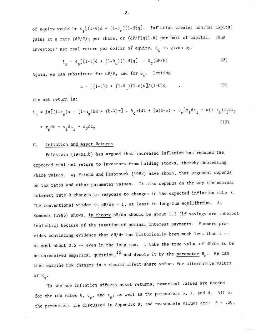
of equity would be ~s[(1-e)d + (l-0c )(l-d)q]. Inflation creates nominal capital

gains at a rate (dP/P)q per share, or (dP/P)q(l-b) per unit of capital. Thus

investors' net real return per dollar of equity, s is given by:

is = [E(l-e)d + (1-ec)(l-d)q] - e (dP/P) (8)

Again, we can substitute for dP/P, and for s. Letting

a = [(l-e)d + (1-e)(1-d)q]/(l-b)q (9)

the net return is:

= {a[(l-T ) - (1- )bR + (b-X)r] - e C}dt + [a(b-X) - e] dz + a(l- e)2dz 2

= rdt + Sldz + dz 2(10)

C. Inflation and Asset Returns

Feldstein (1980a,b) has argued that increased inflation has reduced the

expected real net return to investors from holding stocks, thereby depressing

share values. As Friend and Hasbrouck (1982) have shown, that argument depends

on tax rates and other parameter values. It also depends on the way the nominal

interest rate R changes in response to changes in the expected inflation rate r.

The conventional wisdom is dR/dn = 1, at least in long-run equilibrium. As

Summers (1983) shows, in theory dR/d¶ should be about 1.3 (if savings are interest

inelastic) because of the taxation of nominal interest payments. Summers pro-

vides convincing evidence that dR/d7 has historically been much less than 1 --

at most about 0.6 -- even in the long run. I take the true value of dR/d7 to be

an unresolved empirical question,16 and denote it by the parameter R . We can

then examine how changes in i should affect share values for alternative values

of R

To see how inflation affects asset returns, numerical values are needed

for the tax rates 6, 0c, and Ts, as well as the parameters b, X, and d. All of

the parameters are discussed in Appendix B, and reasonable values are: e = .30,

III

-9-

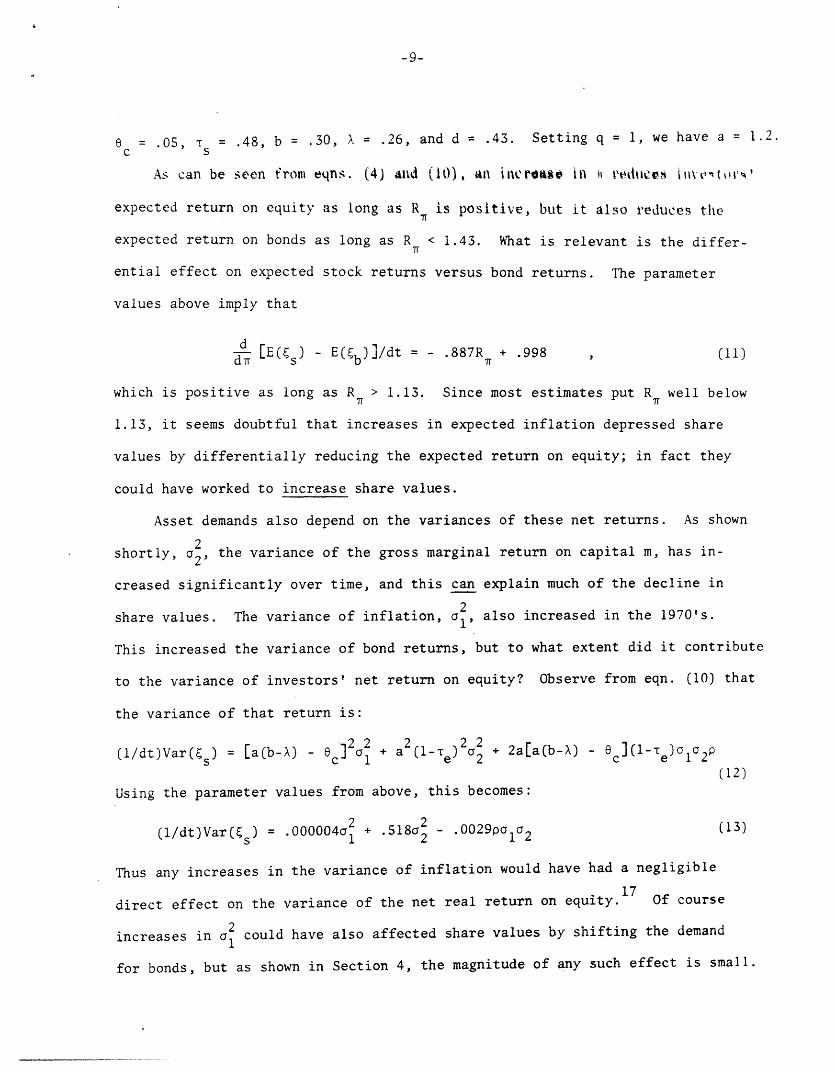
6 = .05, Ts = .48, b = .30, X = .26, and d = .43. Setting q = 1, we have a = 1.2.c

As can be seen tromn eqns. (4) ad (10) , an itreso~ ill i I'dtItcos ilvotlt,''

expected return on equity as long as R is positive, but it also reduces the

expected return on bonds as long as R < 1.43. What is relevant is the differ-

ential effect on expected stock returns versus bond returns. The parameter

values above imply that

d [E() E(b)I/dt = - .887R + .998 (11)

which is positive as long as R > 1.13. Since most estimates put R well below

1.13, it seems doubtful that increases in expected inflation depressed share

values by differentially reducing the expected return on equity; in fact they

could have worked to increase share values.

Asset demands also depend on the variances of these net returns. As shown

shortly, a2, the variance of the gross marginal return on capital m, has in-

creased significantly over time, and this can explain much of the decline in

2share values. The variance of inflation, o1, also increased in the 1970's.

This increased the variance of bond returns, but to what extent did it contribute

to the variance of investors' net return on equity? Observe from eqn. (10) that

the variance of that return is:

(l/dt)Var(Ss) = [a(b-X) - ec] 2 1+ a (1- e )2a2 + 2a[a(b-X) - ](l-e1 )o 2 p- Oc e 2

(12)

Using the parameter values from above, this becomes:

2 213)(l/dt)Var(Es) = .000004a1 + .518a 2 .0029pa2 (13)

Thus any increases in the variance of inflation would have had a negligible

17direct effect on the variance of the net real return on equity. Of course

increases in a2 could have also affected share values by shifting the demand

for bonds, but as shown in Section 4, the magnitude of any such effect is small.

__j___l__Lsjl�__·______Lllll___^l I-�-._�-

-10-

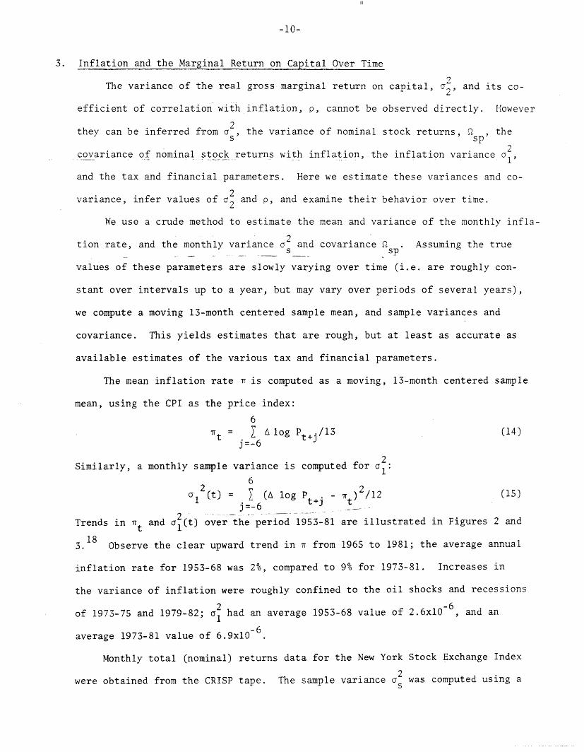
3. Inflation and the Marginal Return on Capital Over Time

The variance of the real gross marginal return on capital, a', and its co-

efficient of correlation with inflation, p, cannot be observed directly. However

2they can be inferred from a , the variance of nominal stock returns, Q p, the

covariance of nominal stock returns with inflation, the inflation variance a1,

and the tax and financial parameters. Here we estimate these variances and co-

variance, infer values of 2 and p, and examine their behavior over time.

We use a crude method to estimate the mean and variance of the monthly infla-

2tion rate, and the monthly variance a and covariance sp Assuming the true

values of these parameters are slowly varying over time (i.e. are roughly con-

stant over intervals up to a year, but may vary over periods of several years),

we compute a moving 13-month centered sample mean, and sample variances and

covariance. This yields estimates that are rough, but at least as accurate as

available estimates of the various tax and financial parameters.

The mean inflation rate is computed as a moving, 13-month centered sample

mean, using the CPI as the price index:

6

it = A log Pt+j/ 3 (14)j=-6

Similarly, a monthly sample variance is computed for a1:

6

2 2a1 (t) = (A log Ptj . -t) /12 (15)

Trends in t and 21(t ) over the period 1953-81 are illustrated in Figures 2 and

3. Observe the clear upward trend in from 1965 to 1981; the average annual

inflation rate for 1953-68 was 2%, compared to 9% for 1973-81. Increases in

the variance of inflation were roughly confined to the oil shocks and recessions

of 1973-75 and 1979-82; a2 had an average 1953-68 value of 2.6x106, and an

average 1973-81 value of 6.9x10 6.

Monthly total (nominal) returns data for the New York Stock Exchange Index

were obtained from the CRISP tape. The sample variance oa was computed using aS

III

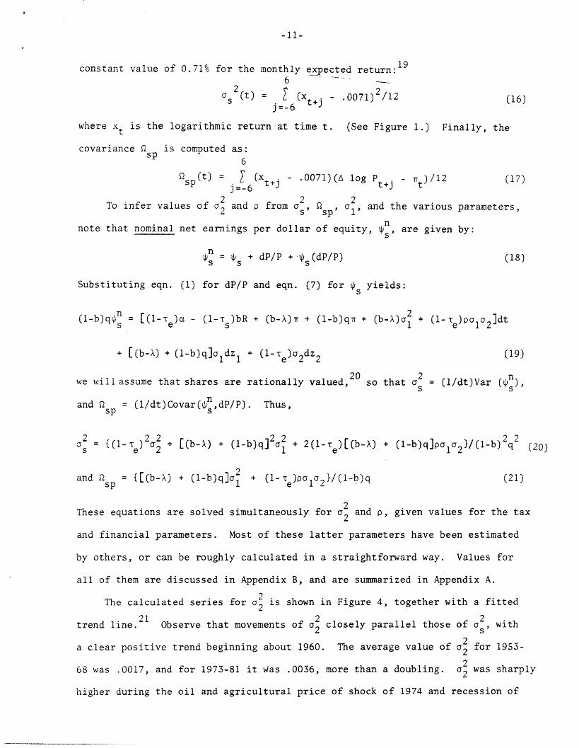
-11-

constant value of 0.71% for the monthly expected return:1 9

6

a (t) = (xt - .0071) 2/12 (16)j=-6

where xt is the logarithmic return at time t. (See Figure 1.) Finally, the

covariance is computed as:sp

2 (t) = Y 112~spt) j= _ (xt+j - .0071)(A log Pt )/12 (17)

j=-62 2 2

To infer values of 2 and p from o S, Sps al, and the various parameters,

nnote that nominal net earnings per dollar of equity, s', are given by:

n

~s = *s + dP/P + s(dP/P) (18)

Substituting eqn. (1) for dP/P and eqn. (7) for s yields:

(1-b)q n = [(1-T e) - (1-s)bR + (b-X)T + (l-b)q + (b-X)a2 + (l-' e)POl2]dt

+ [(b-X) + (l-b)q]oldz 1 + (l-re)a2dz 2 (19)

we will assume that shares are rationally valued,2 0 so that a = (l/dt)Var (),5 5

nand nQp = (l/dt)Covar($ ,dP/P). Thus,

2 22 22 222 = {(1-Te) 2 + [(b-X) + (1-b)q]2a + 2 (1- )[(b-X) + (1-b)q]pola2}/(l-b)2q (20)s e 2(1 e 2

and p [= {(b-X) + (l-b)q]o2 + (1- e)pOlo2}/(l-b)q (21)

2These equations are solved simultaneously for a2 and p, given values for the tax

and financial parameters. Most of these latter parameters have been estimated

by others, or can be roughly calculated in a straightforward way. Values for

all of them are discussed in Appendix B, and are summarized in Appendix A.

The calculated series for a2 is shown in Figure 4, together with a fitted

~~~~21 2 2trend line. Observe that movements of 2 closely parallel those of a2, with2 closely parallel those of as, with

a clear positive trend beginning about 1960. The average value of a2 for 1953-

268 was .0017, and for 1973-81 it as .0036, more than a doubling. a2 was sharply

higher during the oil and agricultural price of shock of 1974 and recession of

-12-

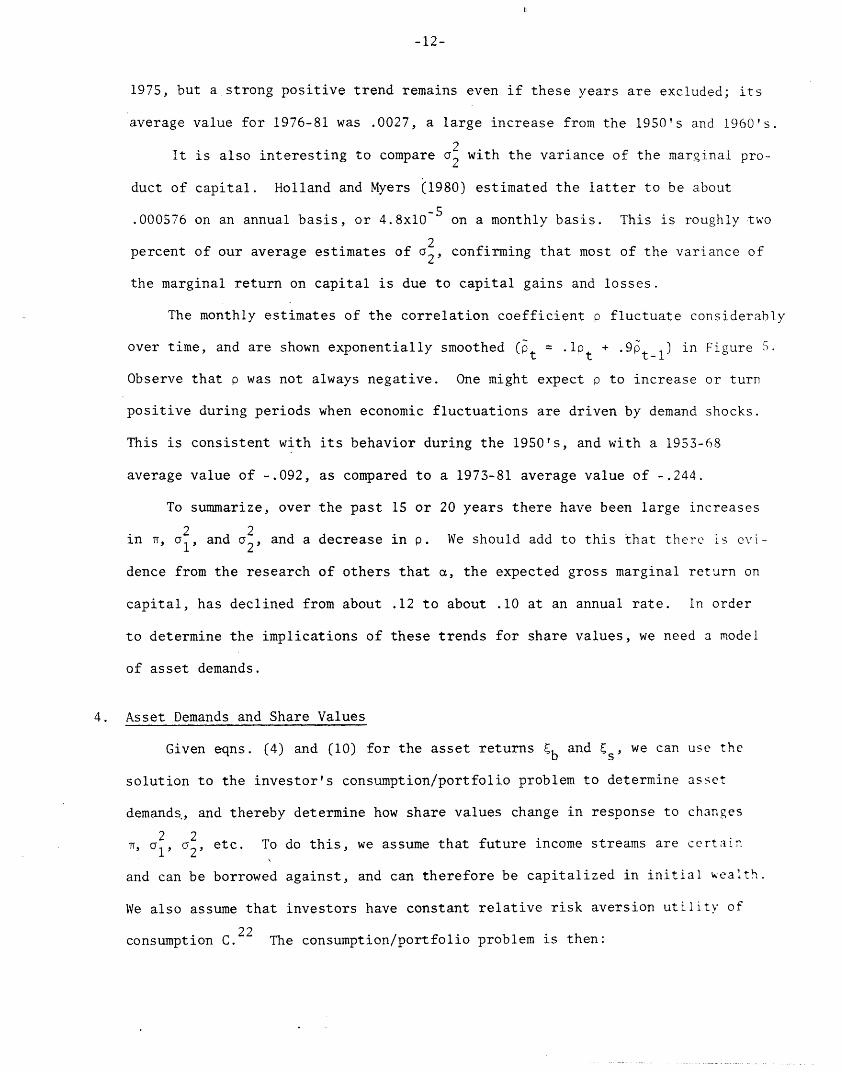
1975, but a strong positive trend remains even if these years are excluded; its

average value for 1976-81 was .0027, a large increase from the 1950's and 1960's.

It is also interesting to compare a2 with the variance of the marginal pro-

duct of capital. Holland and Myers (1980) estimated the latter to be about

.000576 on an annual basis, or 4.8x10 5 on a monthly basis. This is roughly two

2percent of our average estimates of o 2, confirming that most of the variance of

the marginal return on capital is due to capital gains and losses.

The monthly estimates of the correlation coefficient p fluctuate considerably

over time, and are shown exponentially smoothed (Pt = .lot + 9Ptl) in Figure 5.

Observe that p was not always negative. One might expect p to increase or turn

positive during periods when economic fluctuations are driven by demand shocks.

This is consistent with its behavior during the 1950's, and with a 1953-68

average value of -.092, as compared to a 1973-81 average value of -.244.

To summarize, over the past 15 or 20 years there have been large increases

2 2in , a2, and a2, and a decrease in p. We should add to this that there is cvi-

dence from the research of others that a, the expected gross marginal return on

capital, has declined from about .12 to about .10 at an annual rate. In order

to determine the implications of these trends for share values, we need a model

of asset demands.

4. Asset Demands and Share Values

Given eqns. (4) and (10) for the asset returns b and %s, we can use thesolution to the investor's consumption/portfolio problem to determine asset

demands,, and thereby determine how share values change in response to changes

, 1, o2, etc. To do this, we assume that future income streams are certain

and can be borrowed against, and can therefore be capitalized in initial ealth.

We also assume that investors have constant relative risk aversion utility of

consumption C. The consumption/portfolio problem is then:

III

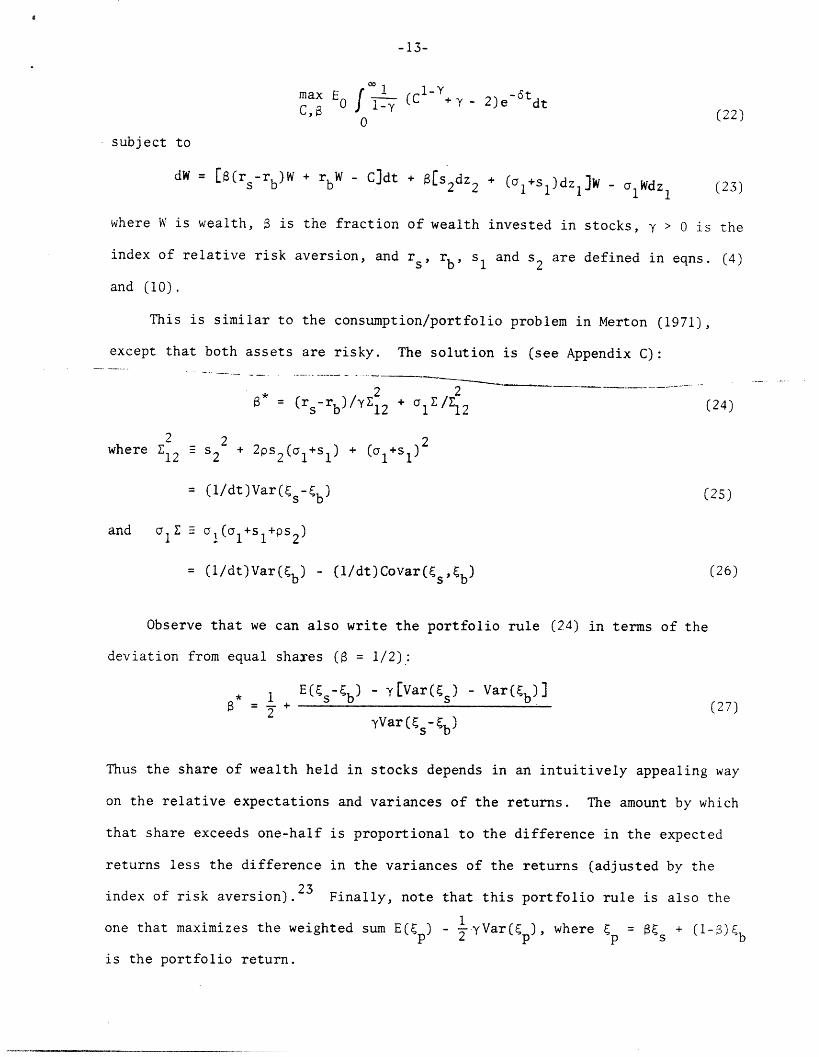
-13-

max E0 I Y (C +y - 2)e dt~c~~,~~~~ i-Y ~~~ (22)

0subject to

dW = [8(rs-rb)W + rW - Cdt + [s2dz + (al+Sl)dl]W Wdz (23)s b b 2 2 1 1 W - c 1Wd(23)

where W is wealth, is the fraction of wealth invested in stocks, y > 0 is the

index of relative risk aversion, and rs, rb, 1 and s2 are defined in eqns. (4)

and (10).

This is similar to the consumption/portfolio problem in Merton (1971),

except that both assets are risky. The solution is (see Appendix C):

*' = (r-rb)/y212 + 1 Z/ 1 2 (24)

2 2 2where 12 S2 + 2ps 2 (a1 +S1

) + (a +S)

(l/dt)Var(Cs-Eb) (25)

and lE oai(al+s 1+ps 2)

= (l/dt)Var(Eb) - (l/dt)Covar(Cs, b) (26)

Observe that we can also write the portfolio rule (24) in terms of the

deviation from equal shaxes ( = 1/2):

* 1 E(is- b) - y[Var(s) - Var(Eb)]

2yVar + (27)¥Var (s-)

Thus the share of wealth held in stocks depends in an intuitively appealing way

on the relative expectations and variances of the returns. The amount by which

that share exceeds one-half is proportional to the difference in the expected

returns less the difference in the variances of the returns (adjusted by the

index of risk aversion). Finally, note that this portfolio rule is also the

one that maximizes the weighted sum E([p) - -yVar(Cp), where ip = is + (1-3)5b

is the portfolio return.

U~~~r_ III_~~~~~~_ _ - --

-14-

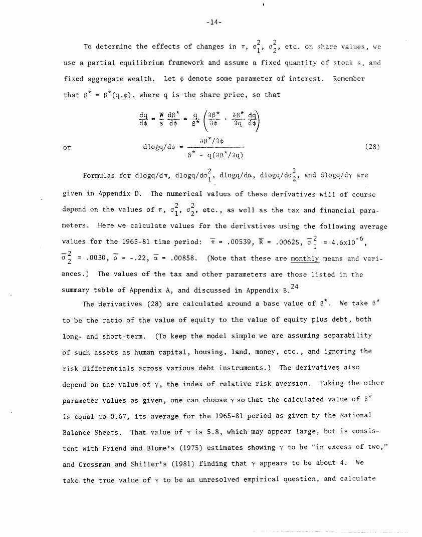
2 2To determine the effects of changes in , ol, 2, etc. on share values, we

use a partial equilibrium framework and assume a fixed quantity of stock s, and

fixed aggregate wealth. Let ~ denote some parameter of interest. Remember

that * = *(q,~), where q is the share price, so that

dq W d qa

dp s d + q q '

a*/a~or dlogq/d = (28)

28 - q(a2*/aq)

Formulas for dlogq/dr, dlogq/da1, dlogq/da, dlogq/da 2, and dlogq/dy are

given in Appendix D. The numerical values of these derivatives will of course

depend on the values of , a1, a2, etc., as well as the tax and financial para-

meters. Here we calculate values for the derivatives using the following average

--2 -6values for the 1965-81 time period: r = .00539, R = 4.6x 1

--22 = .0030, p = -.22, a = .00858. (Note that these are monthly means and vari-

ances.) The values of the tax and other parameters are those listed in the

summary table of Appendix A, and discussed in Appendix B.24

The derivatives (28) are calculated around a base value of 8*. We take *

to be the ratio of the value of equity to the value of equity plus debt, both

long- and short-term. (To keep the model simple we are assuming separability

of such assets as human capital, housing, land, money, etc., and ignoring the

risk differentials across various debt instruments.) The derivatives also

depend on the value of y, the index of relative risk aversion. Taking the other

parameter values as given, one can choose y so that the calculated value of *

is equal to 0.67, its average for the 1965-81 period as given by the National

Balance Sheets. That value of y is 5.8, which may appear large, but is consis-

tent with Friend and Blume's (1975) estimates showing to be "in excess of two,"

and Grossman and Shiller's (1981) finding that y appears to be about 4. We

take the true value of to be an unresolved empirical question, and calculate

- 1 -

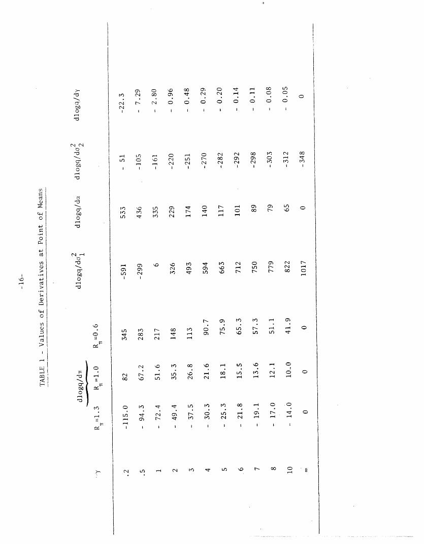
numerical values of the derivatives for alternative values of y. These are shown

in Table 1.

Observe that the sign of dlogq/d7 depends on the value of R . Changes in

affect only expected returns and not their variances or covariance, so from eqn.

(11) dlogq/dT >(<) 0 if R <(>) 1.13. The numbers in Table 1 indicate that

changes in should have a small effect on share values -- unless R is around

.6 or less, as Summers (1983) findings indicate may be the case. If R = 1.0,

an increase in the expected annual inflation rate from 5% to 10% (A1 = .0039)

implies a 7% increase in 2 if y = 5, and a 10% increase if y = 3. However, if

R = .6, the result is a 30% increase in q if y = 5, and a 44% increase if y = 3.

The sign of dlogq/dao depends on y (see eqn. (D.2) in the Appendix). For

2 2our parameter values, dlogq/dao >(<). O if y >(<) .987. An increase in ao

increases the relative riskiness of bonds, but it also increases their expected

return (see eqn. (4)). If y is small enough, the second effect increases the

demand for bonds more than the first reduces it, so that q falls. Since y is

probably greater than one and possibly greater than four, we would expect

dlogq/dal > 0. However, this derivative is small given the average size of a.

In 1973-75 a2 roughly quadrupled from a pre-OPEC average value of about 2x10 6

2 -6(See Figure 3.) This (Aa1 = 6x10 ) implies only a 0.4% increase in q if y = 5

and a 0.3% increase if y = 3.

As we have noted, there is some evidence that a, the expected real gross

marginal return on capital, declined somewhat during the 1970's, perhaps from

.12 to .10 at an annual rate. This decline in a (A = .0015) would imply

an 18% decline in q if y = 5, and a 26% decline if y = 3. This is clearly a

large effect, so even a perceived (as opposed to actual) decline in a could

explain a significant amount of the market's performance.

As we saw in the preceding section, there is evidence that over the past

two decades has more than doubled from an average 1953-68 value of about

;rXAlii�R1%··lk·ar^-·ra^···-·� � ��___

I I I I I CD I I I I O

n D 0 * 0 N N 00 C00 0

_5 z N N n cD N

u: N < *d ' GO

Ln V N- 00 r"T 00 I .4 11 - -

tn N N '-4 1-4

' , ,00

: Ln \LO W CN

0 L( Lf r0'a N 'I LO

\9 l-i Lf~ \D

..4 00 Ln tn

i .1 1-4

b. dz Ln t V 00 -4

N 0h N 0 LO '-

r il I~ tn cI cq I-

N- 0 0Ln 113

r4

0 0O

f-4 C

hi Ln N V r Ln \ O N 0 0 8I- 8

00w0-i

-0

0~u-c

00

-0b0

ci-O

c,

..

OaG)

C,E

C)::1 ,--

-0

co0-o10

0~

04

-0

.O

it

o

r- It

-0 --

II

c..

No D00 'IO

,-4

-17-

.0017 (monthly) to an average 1973-81 value of .0036. This increase in a2 would

~~~~~2 2y = 1. If a2 (or investors' estimates of 2) indeed doubled, this would explain

a large part of the market's decline for any reasonable value of y.

Finally, observe that an increase in y would also have a large negative effect

on share values. For example, an increase in from 4 to 5 would imply a 29%

decline in q. However, we have no evidence that y has changed over time one way or

2 2the other, so our focus in the next section is only on changes in r, a, a, ad a2.

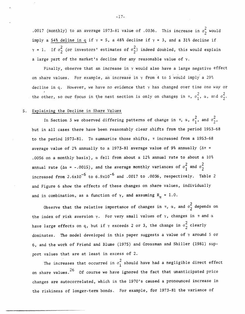
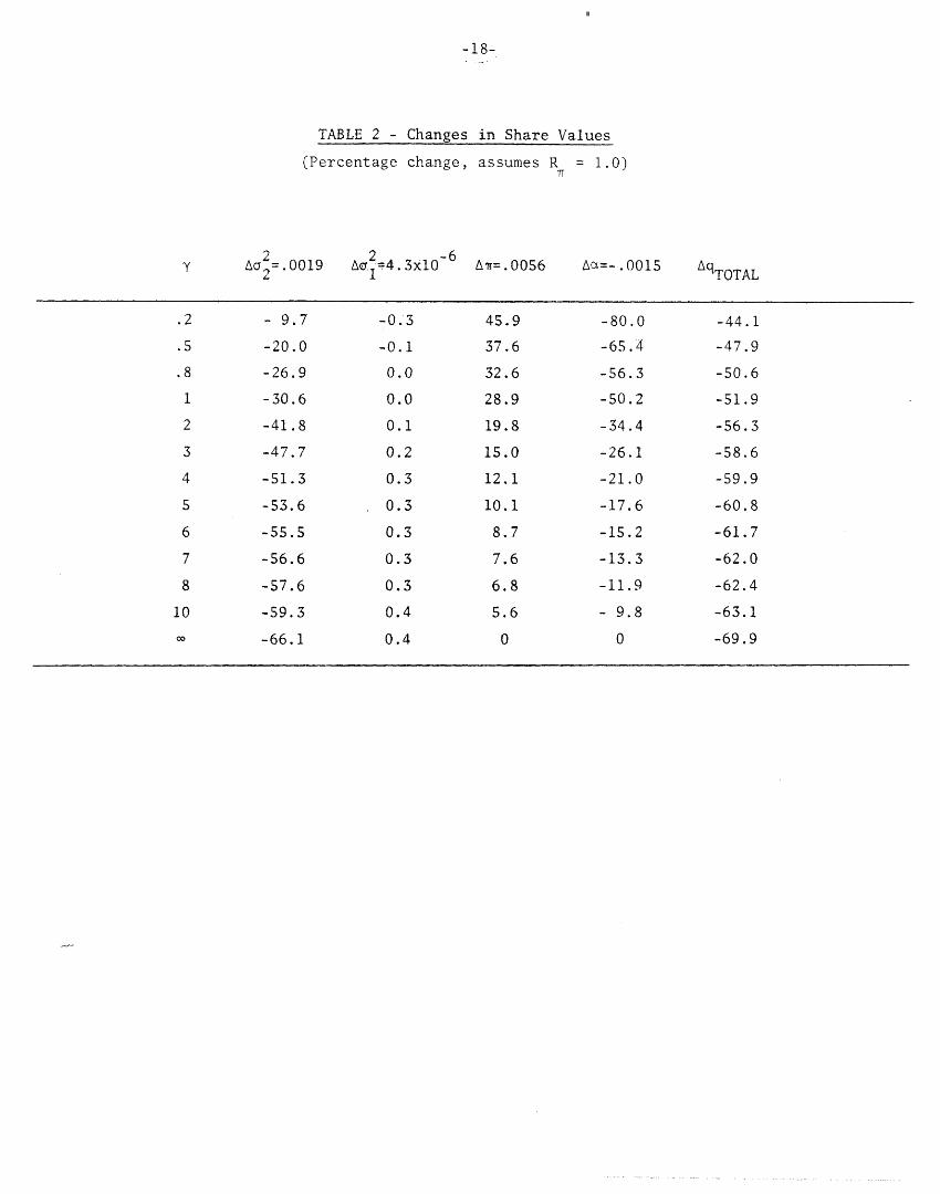
5. Explaining the Decline in Share Values

2 2In Section 3 we observed differing patterns of change in rr, a, al, and 2

but in all cases there have been reasonably clear shifts from the period 1953-68

to the period 1973-81. To summarize those shifts, Tr increased from a 1953-68

average value of 2% annually to a 1973-81 average value of 9% annually (AT =

.0056 on a monthly basis), a fell from about a 12% annual rate to about a 10%

annual rate (Aa = -.0015), and the average monthly variances of a 2 and a2

increased from 2.6x10- 6 to 6.9x10- 6 and .0017 to .0036, respectively. Table 2

and Figure 6 show the effects of these changes on share values, individually

and in combination, as a function of y, and assuming R = 1.0.

Observe that the relative importance of changes in a, a, and a2 depends on

the index of risk aversion y. For very small values of y, changes in and a

have large effects on q, but if y exceeds 2 or 3, the change in 2 clearly

dominates. The model developed in this paper suggests a value of y around 5 or

6, and the work of Friend and Blume (1975) and Grossman and Shiller (1981) sup-

port values that are at least in excess of 2.

The increases that occurred in o1 should have had a negligible direct effect

on share values.26 Of course we have ignored the fact that unanticipated price

changes are autocorrelated, which in the 1970's caused a pronounced increase in

the riskiness of longer-term bonds. For example, for 1973-81 the variance of

Ia� ��_�_��

-18-

TABLE 2 - Changes

(Percentage change,

2 -6Ad.1=4. 3x1OI '.

-0. 3

-0.1

0.0

0.0

0.1

0.2

0.3

0.3

0.3

0.3

0.3

0.4

0.4

in Share Values

assumes R = 1.0)7T

Ar=.00S6

45.9

37.6

32.6

28.9

19.8

15.0

12.1

10.1

8.7

7.6

6.8

5.6

0

Aa=-.0015

-80.0

-65.4

-56.3

-50.2

-34.4

-26.1

-21.0

-17.6

-15.2

-13.3

-11.9

- 9.8

0

2Y Acy2 0019

2

.2

.5

.8

I

2

3

4

5

6

7

8

10

0O

- 9.7

-20.0

-26.9

-30.6

-41.8

-47.7

-51.3

-53.6

-55.5

-56.6

-57.6

-59.3

-66.1

-44.1

-47.9

-50.6

-51.9

-56.3

-58.6

-59.9

-60.8

-61.7

-62.0

-62.4

-63.1

-69.9

-

_ _ _ _ _ __

III

-19-

the real return on 5-year government bonds was about 50 times as large as that

27on 1-month Treasury bills. We can roughly (and conservatively) account for

2 2this in our model by scaling up and Aa by a factor of 50. The value of

dlogq/da2 in Table 1 then falls by about a factor of 5 if = 3, and a factor

of 3 if y = 5 (the other derivatives remain virtually unchanged), so that the

implied increase in q would still not exceed 5%. Thus even if most debt were

longer-term, accounting for autocorrelation would not change this result.

If one accepts that y > 2, then our results point to increased capital risk

as the major cause of the decline in share values. If one believes instead that

y < 2, then the decline in the expected return a stands out as the major explan-

atory factor, although increased capital risk is still important. As for in-

creases in expected inflation, this should have increased share values, unless

R is larger than recent estimates indicate.

6. Concluding Remarks

We have found that much of the decline in share values can be attributed to

the behavior of the gross marginal return on capital. Others have shown that

the expectation of that return has fallen (although there is some controversy

over how much), and this paper has shown that its variance has approximately

doubled. The relative importance of these two changes depends on investors' index

of risk aversion; if that index exceeds 2, increased.risk in the dominating factor.

These results are based on a very simple model of asset returns, asset

demands, and share price determination. Some of the model's limitations have

already been mentioned: the reliance on rational share valuation for the esti-

mation of o2, the assumption of a deterministic income stream in the consumption/

portfolio problem, and the inclusion of only two assets in investors' portfolios.

Even more limiting is the use of a partial equilibrium framework, which ignores

the fact that as q falls the capital stock will begin to fall, and the expected

return a will begin to rise, pushing q back up. Accounting for this would

ss__U____I�___�I__�____

-20-

reduce the magnitude of the derivatives in Table 1, at least for the longer term.

Another issue that requires more attention is how investors' perception of

capital risk should be measured. Our estimates of capital risk are based on

historical fluctuations in stock market returns, i.e. the sample variance of

those returns. The use of survey data might yield better estimates of investors'

perceptions of that risk. For example, investors might believe that there is a

non-negligible probability of economic catastrophe. This would make capital

quite risky, even if stock returns are not very volatile.

Finally, we have implicitly assumed that increases in our estimated values

of a2 reflect actual increases, for whatever reasons, in the riskiness of capital

in the aggregate. Other interpretations are possible once we recognize that

the capital stock is heterogenous. For example, suppose technological change

caused the expected return on riskier capital (i.e. the shares of high-tech

growth firms) to rise. The demand for these riskier stocks would then rise,

increasing the variance of the returns on a value-weighted aggregate stock index,

and possibly leaving share values on average unchanged, or even causing them to

rise.

-21-

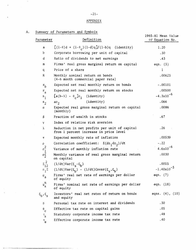
APPENDIX

A. Summary of Parameters and Symbols

Parameter Definition

a [(l-e)d + (1-ec)(1-d)q]/(l-b)q (identity)

b Corporate borrowing per unit of capital

d Ratio of dividends to net earnings

m Firms' real gross marginal return on capital

q Price of a share

R Monthly nominal return on bonds(4-6 month commercial paper rate)

rb Expected net real monthly return on bonds

r Expected net real monthly return on stocks

s1 [a(b-X) - 6 c l1 (identity)

52 au2 (identity)

a Expected real gross marginal return on capital(monthly)

Fraction of wealth in stocks

y Index of relative risk aversion

X Reduction in net profits per unit of capitalfrom 1 percent increase in price level

Expected monthly rate of inflation

p Correlation coefficient: E(dzldz2)/dt

a2l Variance of monthly inflation rate

a2 Monthly variance of real gross marginal returnon capital

E12 (1/dt)Var(Es- b)

o1E (l/dt)Var(Eb) - (l/dt)Covar(%s,Cb)li9s Firms' real net rate of earnings per dollar

of equityn

Firms' nominal net rate of earnings per dollarof equity

ibds Investors' real net rates of return on bondsand equity

e Personal tax rate on interest and dividends

e Effective tax rate on capital gainscStatutory corporate income tax rate

sTr Effective corporate income tax ratee

1965-81 Mean Valueor Equation No.

1.20

.30

.43

eqn. (5)

1

.00625

-. 00101

.00500

-4.3x10

.066

.0086

.67

.26

.00539

-. 22-6

4.6x10

.0030

.0015

-1.40xlO

eqn. (7)

eqn. (18)

eqns. (4), (10)

.30

.05

.48

.40

------- ���,�-�.�I�...-

-22-

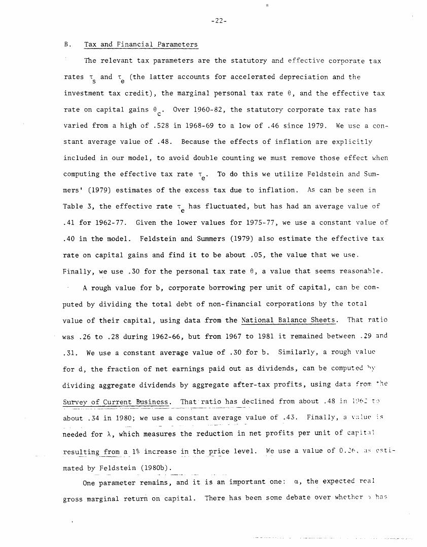
B. Tax and Financial Parameters

The relevant tax parameters are the statutory and effective corporate tax

rates Ts and Te (the latter accounts for accelerated depreciation and the

investment tax credit), the marginal personal tax rate , and the effective tax

rate on capital gains c . Over 1960-82, the statutory corporate tax rate has

varied from a high of .528 in 1968-69 to a low of .46 since 1979. We use a con-

stant average value of .48. Because the effects of inflation are explicitly

included in our model, to avoid double counting we must remove those effect when

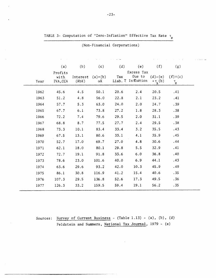
computing the effective tax rate Te . To do this we utilize Feldstein and Sum-

mers' (1979) estimates of the excess tax due to inflation. As can be seen in

Table 3, the effective rate Te has fluctuated, but has had an average value of

.41 for 1962-77. Given the lower values for 1975-77, we use a constant value of

.40 in the model. Feldstein and Summers (1979) also estimate the effective tax

rate on capital gains and find it to be about .05, the value that we use.

Finally, we use .30 for the personal tax rate , a value that seems reasonable.

A rough value for b, corporate borrowing per unit of capital, can be com-

puted by dividing the total debt of non-financial corporations by the total

value of their capital, using data from the National Balance Sheets. That ratio

was .26 to .28 during 1962-66, but from 1967 to 1981 it remained between .29 and

.31. We use a constant average value of .30 for b. Similarly, a rough value

for d, the fraction of net earnings paid out as dividends, can be computed vy

dividing aggregate dividends by aggregate after-tax profits, using data from he

Survey of Current Business. That ratio has declined from about .48 in i16% to

about .34 in 1980; we use a constant average value of .43. Finally, a value is

needed for X, which measures the reduction in net profits per unit of capital

resulting from a 1% increase in the price level. We use a value of 0.26, as esti-

mated by Feldstein (1980b).

One parameter remains, and it is an important one: a, the expected real

gross marginal return on capital. There has been some debate over whether has

-23-

TABLE 3- Computation of "Zero-Inflation" Effective Tax Rate Te

(Non-Financial Corporations)

(b) (c)

Interest (a)+(b)(RbK) caK

4.5

4.8

5.3

6.1

7.4

8.7

10.1

13.1

17.0

18.0

19.1

23.0

29.6

30.8

29.5

33.2

50.1

56.0

63.0

73.8

79.6

77.5

83.4

80.6

69.7

80.1

91.8

101.6

93.2

116.9

136.8

159.5

(d) (e)

Excess Tax

Tax Due toLiab. T Inffl ation

20.6

22.8

24.0

27.2

29.5

27.7

33.4

33.1

27.0

29.8

33.6

40.0

42.0

41.2

52.6

59.4

2.4

2.1

2.0

1.8

2.0

2.4

3.2

4.1

4.8

5.5

6.0

6.9

10.3

15.4

17.3

19.1

Sources: Survey of Current Business - (Table 1.13) - (a), (b), (d)

Feldstein and Summers, National Tax Journal, 1979 - (e)

(a)

Profitswith.

IVA,CCA

45.6

51.2

57.7

67.7

72.2

68.8

73.3

67.5

52.7

62.1

72.7

78.6

63.6

86.1

107.3

126.3

Year

1962

1963

1964

1965

1966

1967

1968

1969

1970

1971

1972

1973

1974

1975

1976

1977

(f)

(d)-(e)+. (b)

20.5

23.2

24.7

28.3

31.1

29.5

35.5

35.9

30.6

32.9

36.8

44.1

45.9

40.6

49.5

56.2

(g)

(f) (c)

e

.41

.41

.39

.38

.39

.38

.43

.45

.44

.41

.40

.43

.49

.35

.36

. 35�---�-

������-�"-�----

-24-

been falling during the past decade or two, and the evidence is mixed, particularly

if a is measured on a cyclically adjusted basis. Using the cyclically adjusted

estimates of a made by Feldstein, Poterba, and Dicks-Mireaux (1981), the average

value for 1962-79 is .11 annual (.00858 monthly). Those estimates suggest that a

has declined from .12 to .10, and we calculate the effect of such a decline on

share values.

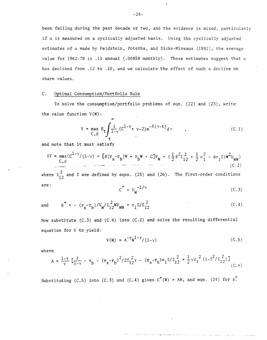
C. Optimal Consumption/Portfolio Rule

To solve the consumption/portfolio problems of eqn. (22) and (23), write

the value function V(W):00

V = max Et fy(C1 -+ y-2)e- 6 (T-t) d (C.1)

t

and note that it must satisfy

+ ( aZ1 2 1 2 26V = max{C /(1-) + [(rs-rb)W + rbW - C]VW + ( 2 2 + - )W V -WW

2 .............. ............... -(C.2)where 12 and are defined by eqns. (25) and (26). The first-order conditions

are: *

C Vw (C.3)

and * (r -rb)/VW/g 2WVww + l /Z12 (C.4)

Now substitute (C.3) and (C.4) into (C.2) and solve the resulting differential

equation for V to yield:

V(W) = A-W 1l-Y/(l-y) (C.5)

where

A -y [' 2 2 - 2 + 2 2 2y 1 - r- b (rSrb) /2 Y -(r r)a 1 (' 12

_8¥Y b s b 12 s b 1 12 ~~~~(C.6)

Substituting (C.5) into (C.3) and (C.4) gives C*(W) = AW, and eqn. (24) for 8*

-25-

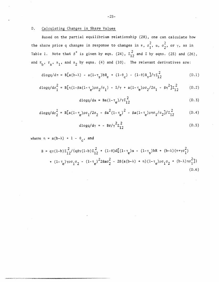
D. Calculating Changes in Share Values

Based on the partial equilibrium relationship (28), one can calculate how

2 2the share price q changes in response to changes in , al , a, o 2, or y, as in

Table 1. Note that * is given by eqn. (24), 2 and by eqns. (25) and (26),12

and rb, r s, 1 , and s2 by eqns. (4) and (10). The relevant derivatives are:

dlogq/d = B[a(b-X) - a(l-Ts)bRI + (1-0c) - (1-e)R ]/yZl2 (D.1)

2 212- c 2 dlogq/dc1 = B[n(l-Sa(l-T )pa2/i1) - l/y + a(l-te)po2/2 1 - 12 (D.2)

dlogq/da = Ba(l- )/E2 (D.3)

dlogq/da2 B[a(l1- )pa /2a -a2 (l- 2 - Sa(l--rT)pn/a]/E (D.4)

2 2dlogq/dy = - Br/y2 22 (D.5)

where n = a(b-X) + 1 - ec, and

B = qy(i-b)Ei2/{qsy(l-b)Z 2 + (l-e)d[(l- e) - (1-TS)bR + (b-X)(T+yc1212lr 12 2 e s

+ (1-T e)YPla 2 - (1-re)22aa2 - 2(a(b-X) + n)(l-e)Pala2 + (b-X)nal1]}

(D.6)

-26-

FOOTNOTES

1. Of course one could argue that no explanation is needed, i.e. the performance of

the market was simply an "unlucky" realization of a stochastic process.

2. It seems hard to believe that such a confusion would persist, particularly during

a decade of high inflation. Also, as Summers (1981a) points out, such confusion

should also have lead to declines in prices of owner-occupied housing.

3. See Friend and Hasbrouck (1982) and Feldstein (1982). Also, Hendershott (1981)

shows that the effect is reduced considerably in a model in which both debt and

equity yields are made endogenous.

4. Changes cited by Malkiel include the return of severe recessions (viewed as a

thing of the past during the 1960's), a higher and more variable inflation rate

(treated explicitly in this paper), and an increase in both the extent and un-

predictability of government regulation.

S. See Bodie (1976), Nelson (1976), and Fama and Schwert (1977).

6. There are good reasons to expect this. For example, supply shocks (e.g. a sudden

increase in the price of oil) tend to create unanticipated inflation and at the

same time reduce the current and expected future marginal products of capital.

Also, as Parks (1978) has shown, unanticipated inflation tends to increase the

dispersion of relative prices. This in turn increases the dispersion of profits

across firms (increasing the risk for each firm), and, if adjustment costs are

significant, reduces expected profits overall. Related to this is Friedman's (1977)

suggestion that unanticipated inflation reduces economic efficiency by magnifying

the distortions caused by government regulation and long-term contracting, and by

reducing the signal-to-noise ratio in the messages transmitted by relative prices.

7. At the end of each year an ARIMA(4,0,0) model is estimated using monthly CPI data

for the preceding 10 years, and is used to forecast the inflation rate for the

next 12 months. I calculate re each year as an average over those 12 months.

Note that ER and e are both measured as monthly rates.

-27-

8. The results are qualitatively the same if my estimated series for the variance of

the marginal return on capital is used instead of a2 The data are described in

Section 3. Black (1976) has shown earlier that stock returns tend to be contem-

poraneously negatively correlated with changes in price volatility.

9. Equation (3) is obtained by use of Ito's Lemma. Fischer (1975) derives eqn. (3),

and also provides a brief introduction to Ito processes such as (1), and Ito's

Lemma and its use. Observe that the greater the variance a 1 of the inflation rate,

the greater the expected real return on the bond. This is just a consequence of

Jensen's inequality; the bond's real price PB/P is a convex function of P.

10. I also assume the nominal interest rate is non-stochastic, so that all of the risk

from holding bonds (apart from default risk) comes from uncertainty over inflation.

As Fama (1975) has shown, this assumption is roughly consistent with the historical

data.

11. Note that a pure discount bond that pays $1 at time T has a present value at time

t of

exp[-jT (R-Tr+c2 )dt + fT'ldz1]t 1 t 1

and therefore a real instantaneous return of (R-r+a2)dt - aldzl, as in eqn. (3)

for the short-term bond.

12. Note that this is apart from the effects of inflation on investors' net real return

that are brought about by the tax system, as explained by Feldstein (1980a,b).

13. In Section 3 we show that the variance of the current marginal product of capital

only accounts for about two percent of the variance of m.

14. This is an approximation, first because losses may more than offset taxable profits

(reducing the effective tax on the stochastic part of m), and second because depre-

ciation allowances are calculated ex ante (increasing the effective tax on the

stochastic part of m). For an analysis of the risk-shifting effects of the

corporate income tax, see Bulow and Summers (1982).

15. I ignore non-interest bearing monetary assets, which are small relative to

interest-bearing debt.

�111�_ __0__�_118____3_1____

-28-

16. In addition to Summers (1983), see Fama (1975) and Nelson and Schwert (1977).

17. This is because a(b-X) . Of course the variance of inflation could have had a

significant indirect effect on the variance of stock returns by partially "ex-

plaining" increases in a2, the variance of m. (See Footnote 6.) We account for

inflation when estimating a2 in Section 3.

18. Inflation was extremely volatile during the Korean War, exceeding 8% during the

first 6 months after the outbreak of the war in July 1950, and dropping to less

than 1% in 1952.

19. This is the mean return for the period 1960-81, and is close to Merton's (1980)

estimate of 0.87% obtained using data for 1926-78. In fact, the expected return

on the market might not be constant; it would change if corporate tax rates

change, if r changes, or if the expected real gross marginal return on capital a

changes. However, as Merton (1980) shows, even if we took this expected return

to be zero, it would bias our estimates of a~ only slightly. Similarly, using a

moving sample mean (as in the computation of a1) makes a negligible difference;

for 1948-81, the monthly series for a computed in this way has a correlation co-

efficient of .981 with the corresponding series computed from eqn. (16). Finally,

note that a2 should ideally be computed using daily data, but such data are

available beginning only in 1962.

20. As Shiller (1981) has shown, the validity of this assumption is questionable.

21. The trend line is:

-2 -4 -6 22 (t) = 7.51x10 + 6.88x10 t. (R = .157)

(3.31) (8.56)

22. Friend and Blume (1975) provide empirical support for this assumption.

23. Because the real gross marginal product of capital is correlated with inflation,

there is no feasible value of p that makes stocks and bonds perfect substitutes

in this model. The assets are perfect substitutes of Z22 = O , but this would

r r 2 1 (lo)21/2s2(sl+o)1 < -10require p = - [ 2 + (S + ) 2 ]/2s (s+a < -1.2 1 121 1

III

-29-

24. These values of p, a, o2, R, , a, and the tax and financial parameters imply

an expected after-tax return to the firm, E(~s), of .629% monthly, or 7.8% annually.

This is well within the range of estimates of the after-tax real rate nf rturn.

25. The evidence is mixed. See Feldstein and Summers (1977), and Feldstein, Poterba,

and Dicks-Mireaux (1981). Holland and Myers (1980) shows a larger decline, from

about 15% to 11%, but do not adjust for cyclical variation.

26. Again, we cannot say whether increases in a1 or indirectly affected share values

by causing part of the decline in a or increase in a2.

27. See Bodie, Kane, and McDonald (1983).

C�I_ � ��

-30-

REFERENCES

1. Black, Fischer, "Studies of Stock Price Volatility Changes," Proceedings of the1976 Meetings of the American Statistical association, Business and Eco-nomic Statistics Section, pp. 177-181.

2. Bodie, Zvi, "Common Stocks as a Hedge Against Inflation," Journal of Finance,31, May 1976, pp. 459-470.

3. Bodie, Zvi, Alex Kane, and Robert McDonald, "Inflation and the Role of Bondsin Investor Portfolios," National Bureau of Economic Research, WorkingPaper No. 1091, March 1983.

4. Bulow, Jeremy I., and Lawrence H. Summers, "The Taxation of Risky Assets,"National Bureau of Economic Research, Working Paper No. 897, June 1982.

5. Fama, Eugene F., "Stock Returns, Real Activity, Inflation, and Money,"American Economic Review, 71, September 1971, pp. 545-565.

6. Fama, Eugene F., "Short-Term Interest Rates as Predictors of Inflation,"American Economic Review, 65, June 1975, pp. 269-282.

7. Fama, Eugene F., and G. William Schwert, "Asset Returns and Inflation,"Journal of Financial Economics, 5, November 1977, pp. 115-146.

8. Feldstein, Martin, "Inflation and the Stock Market," American EconomicReview, 70, December 1980a, pp. 839-847.

9. Feldstein, Martin, "Inflation, Tax Rules, and the Stock Market," Journalof Monetary Economics, 6, 1980b, pp. 309-331.

10. Feldstein, Martin, "Inflation and the Stock Market: Reply," AmericanEconomic Review, 72, March 1982, pp. 243-246.

11. Feldstein, Martin, and Lawrence Summers, "Is the Rate of Profit Falling?"Brookings Papers on Economic Activity, 1977:1, pp. 211-228.

12. Feldstein, Martin, and Lawrence Summers, "Inflation and the Taxation ofCapital Income in the Corporate Sector," National Tax Journal, 32,December 1979, pp. 445-470.

13. Feldstein, Martin, James Poterba, and Louis Dicks-Mireaux, "The EffectiveTax Rate and the Pretax Rate of Return," National Bureau of EconomicResearch, Working Paper No. 740, August 1981.

14. Fischer, Stanley, "The Demand for Index Bonds," Journal of Political Economy,83, June 1975, pp. 509-534.

15. Friedman, Milton, "Nobel Lecture: Inflation and Unemployment," Journal ofPolitical Economy,: 85, June 1977, pp. 451-472.

16. Friend, Irwin, and Marshall E. Blume, "The Demand for Risky Assets," AmericanEconomic Review, 65, December 1975, pp. 900-923.

17. Friend, Irwin, and Joel Hasbrouck, "Inflation and the Stock Market: Comment,"American Economic Review, 72, March 1982, pp. 237-242.

111

-31-

18. Grossman, Sanford J., and Robert J. Shiller, "The Determinants of the Vari-ability of Stock Market Prices," American Economic Review, 71, May1981, pp. 222-227.

19. Hendershott, Patric H., "The Decline in Aggregate Share Values: Taxation,Valuation Errors, Risk, and Profitability," American Economic Review,71, December 1981, pp. 909-922.

20. Holland, Daniel M., and Stewart C. Myers, "Profitability and Capital Costsfor Manufacturing Corporations and All Nonfinancial Corporations,"American Economic Review, 70, May 1980, pp. 320-325.

21. Malkiel, Burton G., "The Capital Formation Problem in the United States,"The Journal of Finance, 34, May 1979, pp. 291-306.

22. Merton, Robert C., "Optimum Consumption and Portfolio Rules in a Continuous-Time Model," Journal of Economic Theory, 3, December 1971, pp. 373-413.

23. Merton, Robert C., "On Estimating the Expected Return on the Market," Journalof Financial Economics, 8, 1980, pp. 323-361.

24. Modigliani, Franco, and Richard Cohn, "Inflation, Rational Valuation, andthe Market," Financial Analysts Journal, 35, March 1979, pp. 3-23.

25. Nelson, Charles R., "Inflation and Rates of Return on Common Stocks," Journalof Finance, 31, May 1976, pp. 471-483.

26. Nelson, Charles R., and G. William Schwert, "On Testing the Hypothesis thatthe Real Rate of Interest is Constant," American Economic Review, 67,June 1977, pp. 478-486.

27. Parks, Richard W., "Inflation and Relative Price Variability," Journal ofPolitical Economy, 86, February 1978, pp. 79-95.

28. Shiller, Robert J., "Do Stock Prices Move Too Much to be Justified by Subse-quent Changes in Dividends?" American Economic Review, 71, June 1981.

29. Summers, Lawrence H., "Inflation, the Stock Market, and Owner-OccupiedHousing," American Economic Review, 71, May 1981a, pp. 429-434.

30. Summers, Lawrence H., "Inflation and the Valuation of Corporate Equities,"National Bureau of Economic Research, Working Paper No. 824, December 1981b.

31. Summers, Lawrence H., "The Non-Adjustment of Nominal Interest Rates: A Studyof the Fisher Effect," in J. Tobin, ed., Macroeconomics, Prices &Quantities, Brookings Institution, 1983.

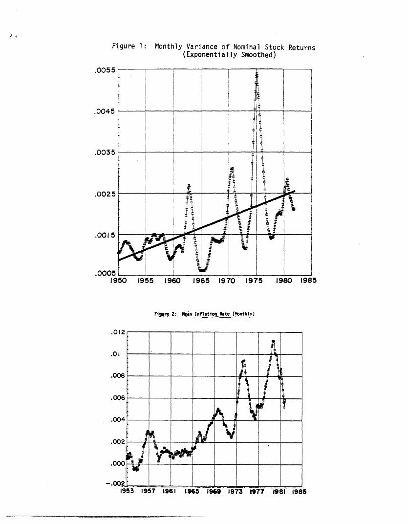
Figure 1: Monthly Variance of Nominal Stock Returns(Exponentially Smoothed)

1955 1960 1965 1970 1975 1980 1985

Fire 2:_ Pan Inflation Rate (Monthly)

2

)8

I6

,4

2

T4 I ~ - . '.

953 I 95 99.. .. 1 ,. ,.. 1

.0055

.0045

.0035

.0025

.0015

.00051950

.01

.01

.00

.00

.00

.00

.00

".00

1953 1957 1965 1969 1973 t977198 19851961

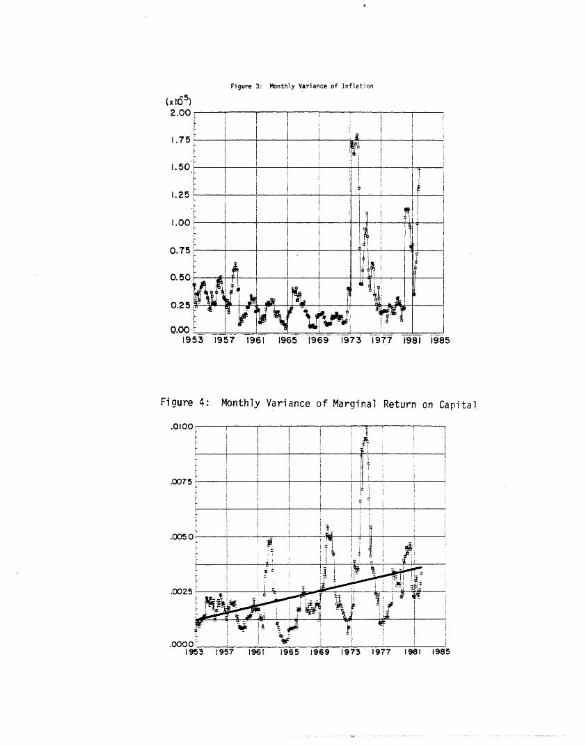
Figure 3: Monthly Variance of Inflation

(xO 5)Z.UU

1.50

1.25

1.00

0.75

0.50

0.25

.0019

Monthly Variance of Marginal Return on Capital

I

Fi ure 4:

AI^

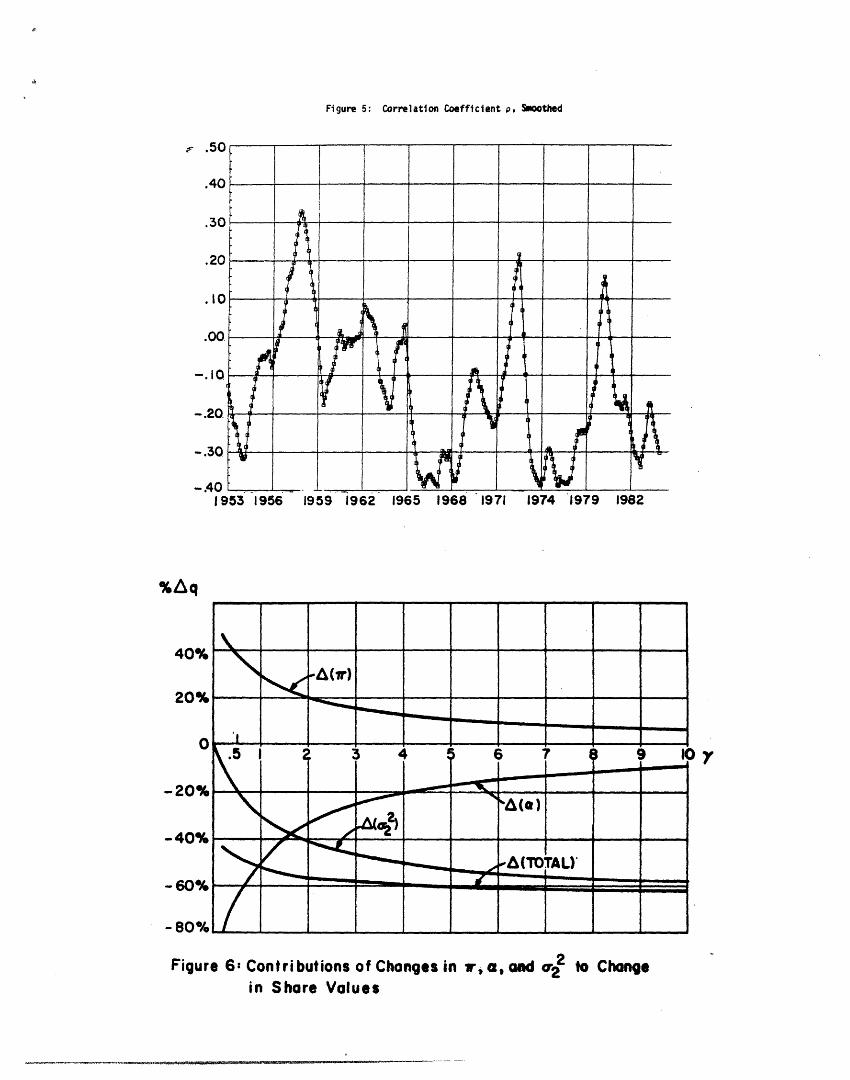
Figure 5: Correlation Coefficient p. Smoothed

t .50

.40

.30

.20

.10

.00

-. 10

- .20

- .30

-.40I

1959 1962 1965 1968 1971V

1974 1979 1982

Figure 6, Contributions of Changes in r, a, ad 02 to Changein Shore Values

%tAq

r'

__

amTI

fI

A

i

I

V_i

I

IF

w -

I�---

I"ri

A

9

--

Ir

I

t I

rI

1953 1956

_W __