Embed Size (px)
Citation preview
DI
SC
US
SI
ON
P
AP
ER
S
ER
IE
S
Forschungsinstitut zur Zukunft der ArbeitInstitute for the Study of Labor
A Big Fish in a Small Pond:Ability Rank and Human Capital Investment
IZA DP No. 9121
June 2015
Benjamin ElsnerIngo E. Isphording
A Big Fish in a Small Pond:
Ability Rank and Human Capital Investment
Benjamin Elsner IZA
Ingo E. Isphording IZA
Discussion Paper No. 9121 June 2015
IZA
P.O. Box 7240 53072 Bonn
Germany
Phone: +49-228-3894-0 Fax: +49-228-3894-180
E-mail: [email protected]
Any opinions expressed here are those of the author(s) and not those of IZA. Research published in this series may include views on policy, but the institute itself takes no institutional policy positions. The IZA research network is committed to the IZA Guiding Principles of Research Integrity. The Institute for the Study of Labor (IZA) in Bonn is a local and virtual international research center and a place of communication between science, politics and business. IZA is an independent nonprofit organization supported by Deutsche Post Foundation. The center is associated with the University of Bonn and offers a stimulating research environment through its international network, workshops and conferences, data service, project support, research visits and doctoral program. IZA engages in (i) original and internationally competitive research in all fields of labor economics, (ii) development of policy concepts, and (iii) dissemination of research results and concepts to the interested public. IZA Discussion Papers often represent preliminary work and are circulated to encourage discussion. Citation of such a paper should account for its provisional character. A revised version may be available directly from the author.
IZA Discussion Paper No. 9121 June 2015
ABSTRACT
A Big Fish in a Small Pond: Ability Rank and Human Capital Investment*
We study the impact of a student’s ordinal rank in a high school cohort on educational attainment several years later. To identify a causal effect, we compare multiple cohorts within the same school, exploiting idiosyncratic variation in cohort composition. We find that a student’s ordinal rank significantly affects educational outcomes later in life. If two students with the same ability have a different rank in their respective cohort, the higher- ranked student is significantly more likely to finish high school, attend college, and complete a 4-year college degree. These results suggest that low-ranked students under-invest in their human capital even if they have a high ability compared to most students of the same age. Exploring potential channels, we find that students with a higher rank have higher expectations about their future career, a higher perceived intelligence, and receive more support from their teachers. JEL Classification: I21, I23, J24 Keywords: human capital, ordinal rank, peer effects, educational attainment Corresponding author: Benjamin Elsner Institute for the Study of Labor (IZA) Schaumburg-Lippe-Str. 5-9 53113 Bonn Germany E-mail: [email protected]
* We would like to thank Peter Arcidiacono, Jan Bietenbeck, Deborah Cobb-Clark, Rajeev Dehejia, Jan Feld, Chris Jepsen, Peter Kuhn, Herb Marsh, Julia Anna Matz, Milena Nikolova, Aderonke Osikominu, Daniele Paserman, Dan Rees, Ying Shi, Derek Stemple, Andreas Steinmayr, Ulf Zölitz, as well as audiences at IZA, RWI, U Mainz, IAB, Modul University, and WU Vienna for helpful comments.
IZA Discussion Paper No. 9121 June 2015
NON-TECHNICAL SUMMARY Parents often believe that high-ability classmates have a positive influence on their children, and potential classmates are often a decisive factor for choosing a school. In this paper, we show that having high-ability peers in school is not beneficial for everyone. A student who is surrounded by peers that are smarter than herself has a low ordinal rank within her peer group, which may come with some disadvantages. While she may benefit from studying with smarter peers, she may experience a disadvantage, for example, because teachers give more attention to higher-ranked students, or because higher-ranked students have a higher self-confidence and higher expectations about their future career. In this paper, we test whether a student’s ordinal rank in a high-school cohort – being the best, second-best, third-best, and so on – affects success in high school, as well as decisions to go to college. We use data from Add Health, a large-scale survey in a representative sample of US high schools, which was administered to 90,000 students in the mid-1990s. In four subsequent waves, these students have been followed until 2008, allowing us to track students from age 16 to age 30, and to link the characteristics of a high-school cohort with educational outcomes many years later. To disentangle the effect of ordinal rank from other factors that could influence educational success – for example, school choice, absolute cognitive ability, parental background, or ethnicity – we compare students who go to the same school and who have the same absolute ability, gender, parental background, etc., but who are in different cohorts. Because not every cohort is the same – some cohorts are smarter than others – a student with the same absolute level of cognitive ability has a different ordinal rank in different cohorts. Overall, we find that a student’s ordinal rank plays an important role for college choices and success in college. We find that in a cohort of 100 students a student who ranks 10 places higher than another is one percentage point more likely to go to college after high-school, and, equally, one percentage point more likely to complete a 4-year college degree. These results suggest that smart students who have a low rank because their peers are even smarter under-invest in their human capital; they choose not to go to college because of their low rank within their cohort. We also give suggestive evidence why rank matters. We find, for example, that students of higher rank have a higher perceived intelligence, and they have higher expectations about their future career. Moreover, students of a higher rank receive more support from their teachers.
1 Introduction
The characteristics of potential classmates are among the decisive factors for parents when
choosing a school for their child. It is commonly believed that children learn and achieve more
when surrounded by high-ability classmates. In this paper, we explore a channel that runs
counter to the positive impact of high-ability peers: a student's ordinal rank in her peer group.
Smart students who have a low relative ability compared to their peer group�small �sh in a big
pond�may erroneously conclude that they have a low absolute ability and, thus, under-invest
in their human capital. Psychologists have labeled this phenomenon the big-�sh-in-a-little-pond
e�ect (Marsh, 1987).
In this paper, we test whether being a big �sh in a high school cohort a�ects the critical
transition from high school to college. Consider two students, Jack and Jim, who have the same
absolute ability, but a di�erent rank in their respective high school cohort: Jack is among the
students with the lowest ability in his cohort, while Jim is among the brightest students in his
cohort. In other words, Jim is a big �sh in a small pond. Here we analyze whether Jim is more
likely than Jack to �nish high school, attend college, and complete a 4-year college degree.
To identify a causal e�ect, we exploit idiosyncratic changes in the cohort composition within
the same school over time. We argue that, conditional on attending a given school, the cohort
composition is exogenous to the student. Entering a school in a given cohort is mainly determined
by a student's birth date and is beyond the in�uence of parents or students.
We use data from the National Longitudinal Study of Adolescent to Adult Health (Ad-
dHealth), a representative survey that tracks students in the US from middle and high school to
their mid-30s, and contains rich information on cognitive skills and educational outcomes. Key
to our identi�cation strategy is that AddHealth covers multiple cohorts within the same high
school, allowing us to exploit the within-school variation in cohort composition. Moreover, the
survey includes an age-speci�c standardized ability test, which makes cognitive ability compa-
rable within and across schools and cohorts. Based on these test scores, we compute a student's
rank as the percentile in the ability distribution of her school cohort.
Our central �nding is that a student's ability rank in a high school cohort has a strong impact
on educational outcomes later in life. A one-decile increase in a student's rank position�the
di�erence between the �rst- and the third-best student in a grade of 20 students�increases
the probability of high-school completion by half a percentage point, and increases both the
probabilities of college attendance and 4-year-degree completion by one percentage point. Given
that cognitive ability, parental education, as well as school and cohort characteristics are held
constant, these are large e�ects. Within a school cohort, the e�ect is non-linear; it is virtually
zero in the lower half of the ability distribution, and strongly positive in the upper half.
While our estimation strategy rules out that the results are driven by selection into schools,
the identi�cation may be threatened by school-speci�c cohort characteristics that are systemati-
cally related to educational attainment. One potential confounder is average peer ability, which
has been shown in many studies to improve student performance. Our baseline speci�cation
2
would not be able to fully disentangle the negative rank e�ect from the positive impact of aver-
age peer ability. To net out the direct in�uence of average cohort characteristics on educational
attainment, we apply a more demanding speci�cation that includes school-by-cohort �xed ef-
fects. This approach absorbs the mean di�erences across cohorts within a school and identi�es
the e�ect only through di�erences in the variance of the ability distribution across cohorts. The
results are unchanged, suggesting that the e�ect of rank on educational attainment is not biased
by school-speci�c cohort characteristics.
In theory, this result can be explained by at least four mechanisms. First, the rank may pro-
vide students with incomplete information of their own absolute ability. Students may conclude
from a low relative ability that they have a low absolute ability. This misperception may distort
the trade-o� between the costs and bene�ts of education. Students may choose not to go to
college if a low perceived ability translates into low expected returns to college. Second, rank can
a�ect intrinsic factors. Students with a higher rank may be more motivated and self-con�dent
and, hence, put more e�ort into their studies, which then translates into a higher chance of going
to college. Third, a student's environment may be responsive to a student's rank. Teachers,
family, and friends may o�er more support to high-ranked students, leading to better grades
and a higher chance of going to college. Finally, the result could be explained by selective col-
lege admission policies. Colleges often observe a student's GPA rank within a cohort, which is
correlated with our rank measure. If admissions o�cers give priority to students with a higher
rank regardless of the school quality, or if colleges automatically admit the top 10% of a school
cohort, then this can explain the e�ect.
While we are not able to fully disentangle these mechanisms, we exploit the rich survey
information in AddHealth to provide suggestive evidence that some channels are more important
than others. We �nd strong evidence for the expected earnings channel. Applying the same
empirical strategy as before, we �nd that a higher rank has an equally large e�ect on various
measures of career expectations at the age of 16 as it has on the actual outcomes 14 years later.
Moreover, we �nd that students with a higher rank are more optimistic, have a higher perceived
intelligence, and put more e�ort into their studies, while we �nd no relationship between rank
and various measures of well-being, happiness, and depression. In terms of support from their
environment, students with a higher rank report a higher perceived support from their teachers,
while the rank is not related to support from parents and friends. Finally, while we have no
information on the type of college to which students are admitted, we can exclude that the
e�ect is purely driven by selective college admissions. When we run our baseline model and
additionally control for GPA, the e�ect of the ability rank on educational attainment remains
large and statistically signi�cant, indicating that GPA-based college admissions explain only a
fraction of the e�ect.
With this paper, we contribute to three strands of the literature. First, this paper extends
the literature on ordinal rank and education outcomes. A large literature in psychology focuses
on a student's academic self-concept, showing that students with a higher ordinal rank have a
higher perceived ability in various school subjects (Marsh, 1987; Marsh et al., 2007). The �rst
3
rigorous causal estimate of ordinal rank on educational performance is provided by Murphy &
Weinhardt (2014), who use administrative school data from the UK, and �nd a strong positive
impact of ordinal rank in primary school on test scores in secondary school. Our paper uses a
very similar research design, but departs from their study in two important dimensions. First,
our data cover a longer time span, allowing us to estimate long-run e�ects of ordinal rank.
Second, in addition to performance, we show that a student's ordinal rank a�ects actual choices
in the transition from high school to college, which are crucial for future careers.
More broadly, this paper speaks to the literature on peer e�ects in education. So far, there is
no consensus if and to what extent peers matter for student performance. While earlier studies
have found that higher peer quality has a positive impact on test scores and a�ects later education
choices, more recent studies show that peer e�ects are non-linear and can even be negative for
some students.1 The ordinal rank e�ect found in this paper provides one explanation for these
ambiguous e�ects. The positive e�ect of having better peers can be o�set by having a lower
ordinal rank.
This paper also contributes to the literature on imperfect information and educational
choices. The evidence shows that students have imperfect knowledge of their own ability (Stine-
brickner & Stinebrickner, 2012, 2014; Zafar, 2011; Bobba & Frisancho, 2014) and are uncertain
about their returns to education (Jensen, 2010; Attanasio & Kaufmann, 2015; Wiswall & Zafar,
2015). Our results suggest that the ordinal rank is one of the reasons why students have in-
correct beliefs about their absolute ability. In their education decisions, students seem to place
substantial weight on their relative ability, which leads to suboptimal education choices.
2 Data and Descriptive Statistics
2.1 The AddHealth data
Our data is the restricted-use version of AddHealth, a representative longitudinal dataset of
US middle and high schools. Four features of AddHealth are key to our study: �rst, it covers
multiple cohorts within the same school. This is critical for identi�cation, because we can
compare students in adjacent cohorts within the same school, and exclude selection into schools
as a main confounding factor. Second, within every school cohort, we observe a representative
sample of students from which we can construct the ability ranking. Third, the longitudinal
set-up allows us to link the ordinal rank in high school to outcomes 14 years later and to observe
the critical transition from high school to tertiary education. Finally, the survey includes a
standardized test that provides us with an objective measure of cognitive ability. Unlike in most
1 The evidence for positive peer e�ects on student performance ranges from primary schools (Hanushek et al.,2003; Ammermueller & Pischke, 2009) to high schools (Calvó-Armengol et al., 2009; Imberman et al., 2012)to college (Sacerdote, 2001; Zimmerman, 2003; Carrell et al., 2009; De Giorgi & Pellizzari, 2014; Booij et al.,2015). Bifulco et al. (2011) and Patacchini et al. (2012) show that better peers also increase the likelihoodof going to college. Studies that �nd a non-linear e�ect or zero e�ect are Lavy et al. (2012), Koppensteiner(2012), Carrell et al. (2013), Burke & Sass (2013), Pop-Eleches & Urquiola (2013), Abdulkadiroglu et al.
(2014), Feld & Zölitz (2014), Tincani (2015) and Tatsi (2015).
4
other datasets, we can directly measure cognitive ability without having to resort to grades or
other self-reported measures as proxies.
To date, four waves of AddHealth are available. The �rst wave was administered in 1994/1995,
when students were between 13 and 18 years old. Follow-ups were run in 1996, in 2000/2001
when most students had left high school, and in 2008/2009, when most had entered the labor
market. In the �rst wave, a representative sample was drawn among all public and private
high schools in the US. Within each school, students from grades 7-12 were sampled. In total,
we observe up to six cohorts within a school. All cohorts were interviewed at the same time;
therefore, we only observe each cohort in one grade, i.e., we observe the 1994 entry cohort in
grade 7, the 1993 entry cohort in grade 8, the 1992 entry cohort in grade 9, etc. Given that we
observe each cohort only in one grade, we will use cohort and grade interchangably.2
The �rst wave consisted of two questionnaires: a basic In-school questionnaire, which was
administered to all students in the surveyed schools, and a more comprehensive In-home ques-
tionnaire, which was answered by a randomly drawn subsample of students within each school.
For the In-home sample, 17 boys and 17 girls were randomly drawn from each grade within
each school. Additional students were drawn to oversample groups with certain characteris-
tics: twins, students with disabilities, Blacks from well-educated families, as well as students of
Chinese, Cuban, and Puerto Rican origin.3
Our main sample is the In-home sample of the �rst wave, which we complement with
information on the educational attainment from the fourth wave. We drop from the sample all
schools with 20 observations or less (109 obs.) and all grades with 5 students or less (304 obs.).
Moreover, due to attrition, we drop all students for whom we do not observe the educational
attainment (�nished high school, attended any type of college, completed college) or other
observable characteristics in wave IV (4,711 obs.). In total, our sample consists of 13,645 students
in 130 schools and 432 grades.
2.2 Outcome variables: Educational attainment
We consider three outcome variables that measure di�erent degrees of educational attainment:
completed high school, attended college, completed a 4-year college degree. These measures are
taken from wave IV of AddHealth, where respondents were asked about their highest educational
attainment. The categories attended college and completed a 4-year college degree are nested;
completed a 4-year college degree only includes students who completed at least a Bachelor's
degree, while attended college is broader and also includes students who attended college but
�nished with less than a Bachelor's, or did not �nish at all.
Table 1 summarizes the outcome variables for various groups. Among all students, 93%
2 In schools that integrate high- and middle schools and that o�er grades 7 to 12, all grades were sampled.In high schools that only o�er grades 9-12, grades 7 and 8 were sampled from a random middle school(so-called feeder school) that was drawn from all surrounding middle schools that send students to the givenhigh school. For further information on the study design and the sampling, see Harris (2009) and Harriset al. (2009).
3 In 16 so-called saturated schools, all students that were present on the day of the survey were included.
5
completed high school, while 67% attended college. Around half of those who attended college
�nished at least with a Bachelor's degree.4
Across subgroups, the educational attainment di�ers considerably. In all three measures,
women have a higher educational attainment than men. The data also reveal a high correlation
between the educational attainment of the parents and their children. Children of college-
educated parents are four times as likely to complete a college degree and ten times less likely
to drop out of high school than children whose parents were high school dropouts. There is less
variation in the educational attainment across ethnic groups. Hispanics and Blacks have lower
educational attainment than Whites, but the raw di�erences are less than 10 percentage points.
An exception are students of Asian descent, whose educational attainment is considerably higher
than in all other groups.
Finally, we consider schools with di�erent average ability and heterogeneity. Unsurpris-
ingly, students from schools in the top half have a higher educational attainment. We also
check if more heterogeneous schools are more or less conducive to educational success. If schools
are homogeneous with respect to ability, for example, because of tracking or because of neigh-
borhood segregation, one would expect homogeneous schools to have di�erent outcomes than
heterogeneous schools. The raw data, however, do not support this conjecture.
2.3 Ranking students
The regressor of interest is a student's ordinal rank in the ability distribution of a high-school
cohort. We are interested in estimating a causal e�ect of rank on educational outcomes, which
we identify by comparing students within the same school and with the same level of absolute
ability who di�er in their ordinal rank because they are in di�erent cohorts. This identi�cation
strategy requires a standardized ability test that makes students comparable across cohorts
within the same school. To obtain a standardized measure of cognitive ability, we use the
scores of a standardized Peabody Picture Vocabulary Test, of which a shortened version was
included in the survey. The test works as follows: participants are asked to allocate words spoken
aloud by the interviewer to a set of four pictures. The test proceeds through multiple rounds
with increasing di�culty. The test is age-speci�c, with test scores being standardized to mean
100 and standard deviation 15 within an age group. The scores are computed automatically,
without being made available to the interviewer or the respondent.5 Though measuring very
basic cognitive skills, the Peabody test has been shown to have a high re-test reliability and
correlates highly with other intelligence tests for adolescents (Dunn & Dunn, 2007).
Based on the Peabody score, we compute a student's ordinal rank as her percentile in the
ability distribution of her school cohort. If a grade has 100 students, the student with the highest
4 These numbers con�rm the representativeness of the survey, as they are very close to the means in theAmerican Community Survey (ACS): 91% have completed high school, 64% attended any type of college,and 31% completed a 4-year degree. These calculations are based on the 2007-2011 Public Use File ofindividuals born between 1976 and 1982 (US natives and immigrants who arrived before 1995).
5 Further information on the Addhealth Picture Vocabulary Test is available in the AddHealth documentationat http://www.cpc.unc.edu/projects/addhealth/data/guides.
6
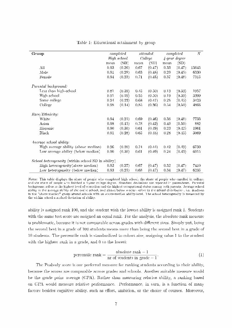
Table 1: Educational attainment by group
Group completed attended completed NHigh school College 4-year degreemean (SD) mean (SD) mean (SD)
All 0.93 (0.26) 0.67 (0.47) 0.33 (0.47) 13645Male 0.91 (0.28) 0.63 (0.48) 0.29 (0.45) 6330Female 0.94 (0.23) 0.71 (0.45) 0.37 (0.48) 7315
Parental background:Less than high-school 0.81 (0.39) 0.45 (0.50) 0.13 (0.33) 1957High school 0.91 (0.29) 0.55 (0.50) 0.19 (0.39) 3399Some college 0.94 (0.23) 0.68 (0.47) 0.28 (0.45) 3423College 0.98 (0.14) 0.85 (0.36) 0.54 (0.50) 4866
Race/Ethnicity:White 0.94 (0.25) 0.69 (0.46) 0.36 (0.48) 7733Asian 0.98 (0.15) 0.78 (0.42) 0.49 (0.50) 882Hispanic 0.90 (0.30) 0.61 (0.49) 0.23 (0.42) 1961Black 0.91 (0.28) 0.65 (0.48) 0.28 (0.45) 3069
Average school ability:High average ability (above median) 0.96 (0.20) 0.74 (0.44) 0.42 (0.49) 6730Low average ability (below median) 0.90 (0.30) 0.61 (0.49) 0.24 (0.43) 6915
School heterogeneity (within-school SD in ability)High heterogeneity(above median) 0.92 (0.27) 0.67 (0.47) 0.32 (0.47) 7410Low heterogeneity (below median) 0.93 (0.25) 0.68 (0.47) 0.34 (0.47) 6235
Notes: This table displays the share of people who completed high school, the share of people who enrolled in college,and the share of people who �nished a 4-year college degree. Standard deviations are reported in parentheses. Parentalbackground refers to the highest level of education and the highest occupational status among both parents. Average schoolability is the average ability of the entire school, and above/below median refers to the school distribution, i.e. studentsin the "above median" group attend schools with an above-median ability-level. The school heterogeneity is measured bythe within-school standard deviation of ability.
ability is assigned rank 100, and the student with the lowest ability is assigned rank 1. Students
with the same test score are assigned an equal rank. For the analysis, the absolute rank measure
is problematic, because it is not comparable across grades with di�erent sizes. Simply put, being
the second best in a grade of 100 students means more than being the second best in a grade of
10 students. The percentile rank is standardized to cohort size, assigning value 1 to the student
with the highest rank in a grade, and 0 to the lowest:
percentile rank =absolute rank− 1
nr of students in grade− 1. (1)
The Peabody score is our preferred measure for ranking students according to their ability,
because the scores are comparable across grades and schools. Another suitable measure would
be the grade point average (GPA). Rather than measuring relative ability, a ranking based
on GPA would measure relative performance. Performance, in turn, is a function of many
factors besides cognitive ability, such as e�ort, ambition, or the choice of courses. Moreover,
7
within many schools, GPAs are not comparable across cohorts because students are graded on
a curve�the same grade distribution is applied within every subject�or grading may depend
on the individual teacher.
But are students aware of their ability rank, that is, do students know their own ability
compared to the ability of others in the same cohort? While we cannot directly infer students'
knowledge of their exact ranks from the survey, we have two pieces of evidence that suggest that
students have an idea about their relative ability in their cohort. First, students with the same
absolute ability but a higher ordinal rank have a higher perceived intelligence. When asked
if they believe that they are more intelligent than the average, students of a higher rank are
signi�cantly more likely to agree than students of lower rank, after controlling for own ability,
personal characteristics, and only comparing students within schools across cohorts. A second
piece of evidence is that students of higher rank have higher expectations about their educational
career. For example, they are more likely to expect to �nish a college degree later in life. This
would hardly be the case if students had no idea about their relative ability.
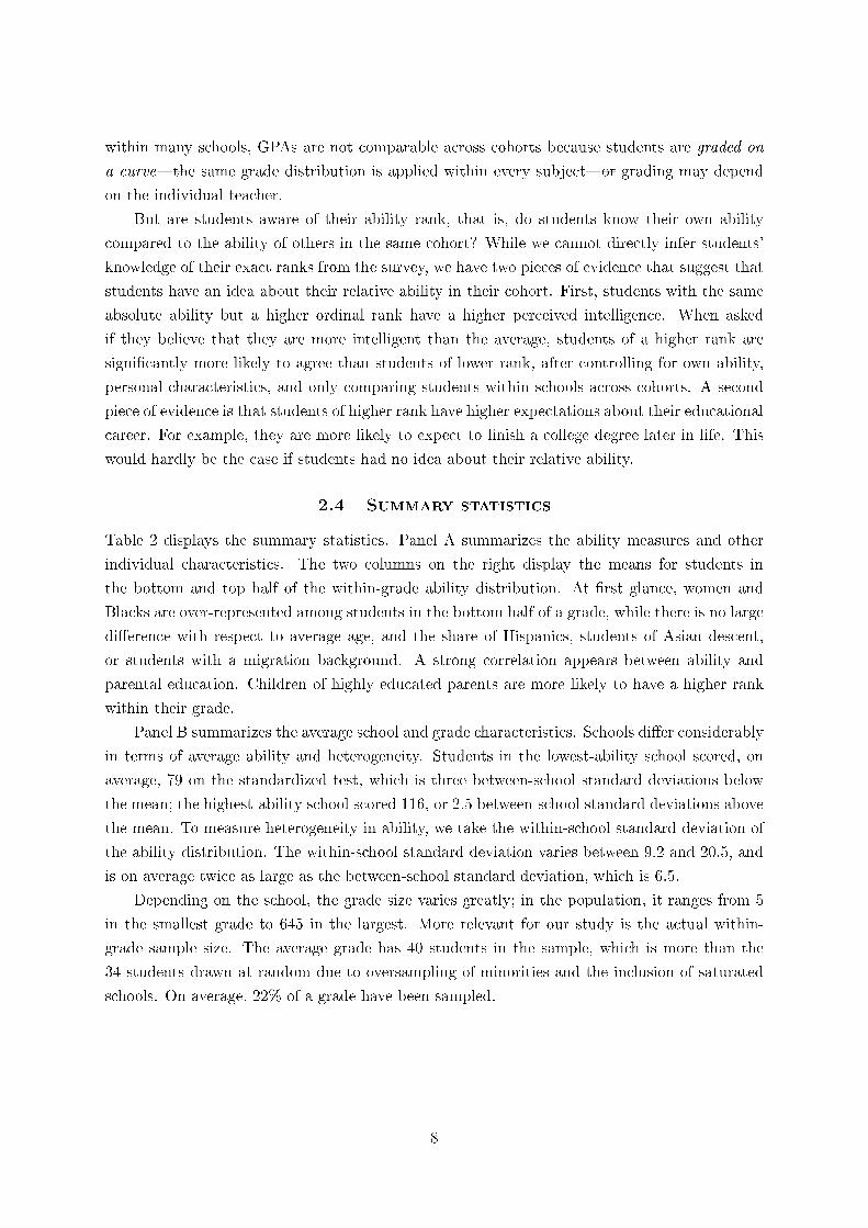
2.4 Summary statistics
Table 2 displays the summary statistics. Panel A summarizes the ability measures and other
individual characteristics. The two columns on the right display the means for students in
the bottom and top half of the within-grade ability distribution. At �rst glance, women and
Blacks are over-represented among students in the bottom half of a grade, while there is no large
di�erence with respect to average age, and the share of Hispanics, students of Asian descent,
or students with a migration background. A strong correlation appears between ability and
parental education. Children of highly educated parents are more likely to have a higher rank
within their grade.
Panel B summarizes the average school and grade characteristics. Schools di�er considerably
in terms of average ability and heterogeneity. Students in the lowest-ability school scored, on
average, 79 on the standardized test, which is three between-school standard deviations below
the mean; the highest-ability school scored 116, or 2.5 between-school standard deviations above
the mean. To measure heterogeneity in ability, we take the within-school standard deviation of
the ability distribution. The within-school standard deviation varies between 9.2 and 20.5, and
is on average twice as large as the between-school standard deviation, which is 6.5.
Depending on the school, the grade size varies greatly; in the population, it ranges from 5
in the smallest grade to 645 in the largest. More relevant for our study is the actual within-
grade sample size. The average grade has 40 students in the sample, which is more than the
34 students drawn at random due to oversampling of minorities and the inclusion of saturated
schools. On average, 22% of a grade have been sampled.
8
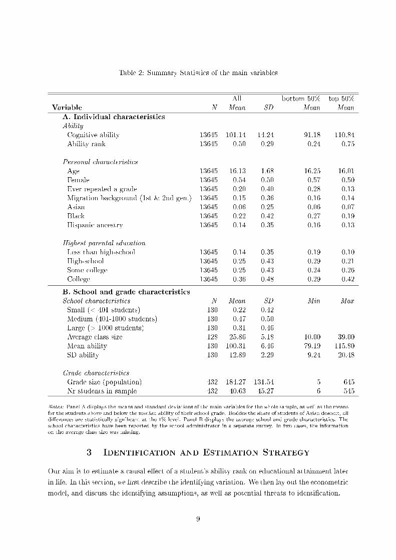
Table 2: Summary Statistics of the main variables
All bottom 50% top 50%Variable N Mean SD Mean Mean
A. Individual characteristics
AbilityCognitive ability 13645 101.14 14.24 91.18 110.84Ability rank 13645 0.50 0.29 0.24 0.75
Personal characteristicsAge 13645 16.13 1.68 16.25 16.01Female 13645 0.54 0.50 0.57 0.50Ever repeated a grade 13645 0.20 0.40 0.28 0.13Migration background (1st & 2nd gen.) 13645 0.15 0.36 0.16 0.14Asian 13645 0.06 0.25 0.06 0.07Black 13645 0.22 0.42 0.27 0.19Hispanic ancestry 13645 0.14 0.35 0.16 0.13
Highest parental educationLess than high-school 13645 0.14 0.35 0.19 0.10High-school 13645 0.25 0.43 0.29 0.21Some college 13645 0.25 0.43 0.24 0.26College 13645 0.36 0.48 0.29 0.42
B. School and grade characteristics
School characteristics N Mean SD Min MaxSmall (< 401 students) 130 0.22 0.42Medium (401-1000 students) 130 0.47 0.50Large (> 1000 students) 130 0.31 0.46Average class size 128 25.86 5.18 10.00 39.00Mean ability 130 100.31 6.46 79.19 115.80SD ability 130 12.89 2.29 9.24 20.48
Grade characteristicsGrade size (population) 432 184.27 131.54 5 645Nr students in sample 432 40.63 45.27 6 545
Notes: Panel A displays the means and standard deviations of the main variables for the whole sample, as well as the meansfor the students above and below the median ability of their school grade. Besides the share of students of Asian descent, alldi�erences are statistically signi�cant at the 1%-level. Panel B displays the average school and grade characteristics. Theschool characteristics have been reported by the school administrator in a separate survey. In two cases, the informationon the average class size was missing.
3 Identification and Estimation Strategy
Our aim is to estimate a causal e�ect of a student's ability rank on educational attainment later
in life. In this section, we �rst describe the identifying variation. We then lay out the econometric
model, and discuss the identifying assumptions, as well as potential threats to identi�cation.
9
3.1 Identifying variation
To estimate a causal e�ect, we exploit idiosyncratic variation in cohort composition within the
same school over time. The idea is that students with the same level of absolute abilty have a
di�erent rank if they are in cohorts with di�erent ability distributions. The variation in cohort
composition can be due to di�erences in mean ability�some cohorts are on average brighter
than others. It can also be due to di�erences in the dispersion of ability within a cohort�in
some cohorts the ability is more evenly distributed than in others. Figure 1, panel (A) illustrates
the identifying variation based on di�erences in mean ability for two entry cohorts in the same
school, each consisting of 4 students. The 1994 entry cohort has a lower average ability, such
that a student with cognitive ability abil would have the second rank. If she entered the school
in 1995, when the entry cohort was stronger, she would only have the third rank, despite having
the same cognitive ability.
Figure 1: Identifying variation: a student with ability=abil has rank 1 in the entry cohort in1994 but rank 2 in 1995. Identi�cation based on (a) di�erences in means or (b) di�erences inshape of ability distribution
By only using variation within schools, we can rule out that the variation in cohort com-
position is driven by systematic self-selection of students into schools.6 But within a school,
where could the di�erences in the ability distribution across cohorts come from? As explained
6 In fact, there is evidence that parents strategically choose schools with their kids' rank in mind. Cullenet al. (2013) show that after automatic admission to the �agship state universities in Texas was granted tothe top 10% of a school, parents deliberately sent their kids to lower-ability schools in order to give them ahigher chance of being in the top 10%.
10
by Hoxby (2000a), one source of variation is the timing of births in combination with a cuto�
date between school years. If in some years more children are born before the age cut-o� than
in others, this leads to �uctuations in the cohort sizes within the same school. Along the same
lines, the characteristics of parents may �uctuate from year to year. In some years, the share of
children born to highly educated parents is higher than in others, the share of Black or Hispanic
children is higher than in others, or in some years more children with a higher innate ability are
born than in others. Due to the law of large numbers, such �uctuations may not be pronounced
in the entire US or in one state, but they are more pronounced within a school district, where
the law of large numbers does not necessarily hold. Our identi�cation relies on this idiosyncratic
variation in the population.
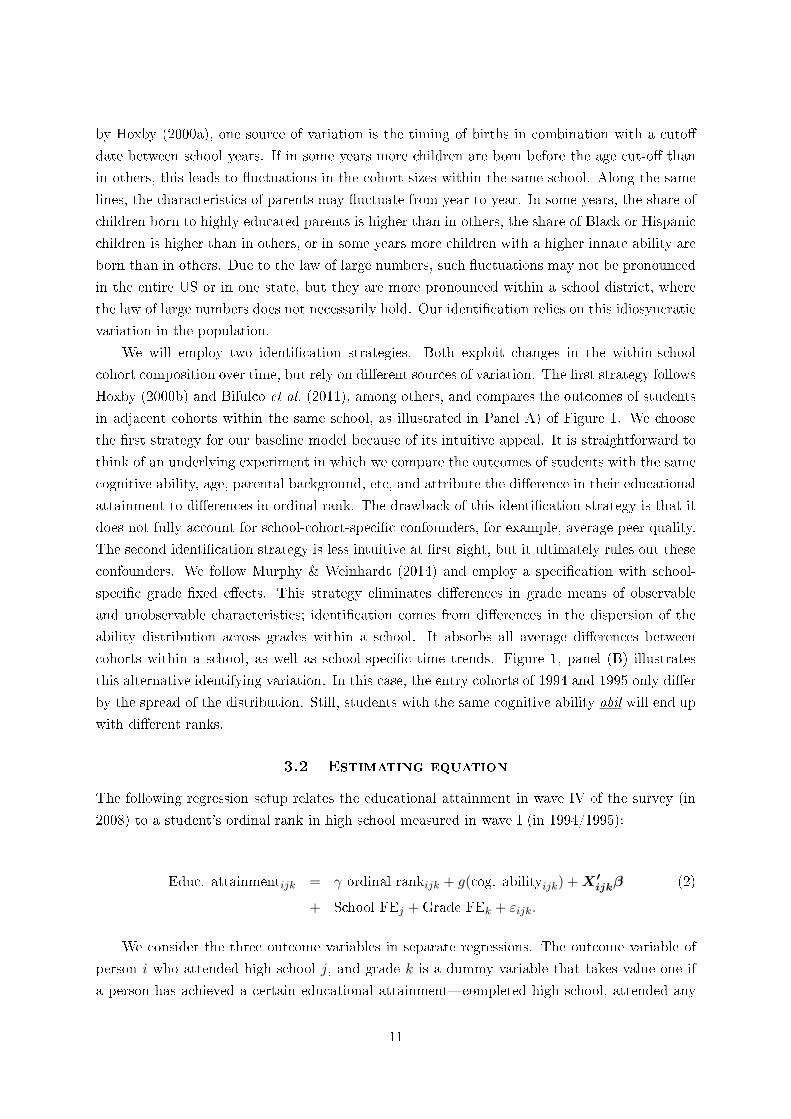
We will employ two identi�cation strategies. Both exploit changes in the within-school
cohort composition over time, but rely on di�erent sources of variation. The �rst strategy follows
Hoxby (2000b) and Bifulco et al. (2011), among others, and compares the outcomes of students
in adjacent cohorts within the same school, as illustrated in Panel A) of Figure 1. We choose
the �rst strategy for our baseline model because of its intuitive appeal. It is straightforward to
think of an underlying experiment in which we compare the outcomes of students with the same
cognitive ability, age, parental background, etc, and attribute the di�erence in their educational
attainment to di�erences in ordinal rank. The drawback of this identi�cation strategy is that it
does not fully account for school-cohort-speci�c confounders, for example, average peer quality.
The second identi�cation strategy is less intuitive at �rst sight, but it ultimately rules out these
confounders. We follow Murphy & Weinhardt (2014) and employ a speci�cation with school-
speci�c grade �xed e�ects. This strategy eliminates di�erences in grade means of observable
and unobservable characteristics; identi�cation comes from di�erences in the dispersion of the
ability distribution across grades within a school. It absorbs all average di�erences between
cohorts within a school, as well as school-speci�c time trends. Figure 1, panel (B) illustrates
this alternative identifying variation. In this case, the entry cohorts of 1994 and 1995 only di�er
by the spread of the distribution. Still, students with the same cognitive ability abil will end up
with di�erent ranks.
3.2 Estimating equation
The following regression setup relates the educational attainment in wave IV of the survey (in
2008) to a student's ordinal rank in high school measured in wave I (in 1994/1995):
Educ. attainmentijk = γ ordinal rankijk + g(cog. abilityijk) +X′ijkβ (2)
+ School FEj +Grade FEk + εijk.
We consider the three outcome variables in separate regressions. The outcome variable of
person i who attended high school j, and grade k is a dummy variable that takes value one if
a person has achieved a certain educational attainment�completed high school, attended any
11
college, or completed a 4-year degree�and zero otherwise. The coe�cient of interest is γ, which
measures the impact of a marginal increase in the percentile rank of a student within a high
school cohort on educational attainment.
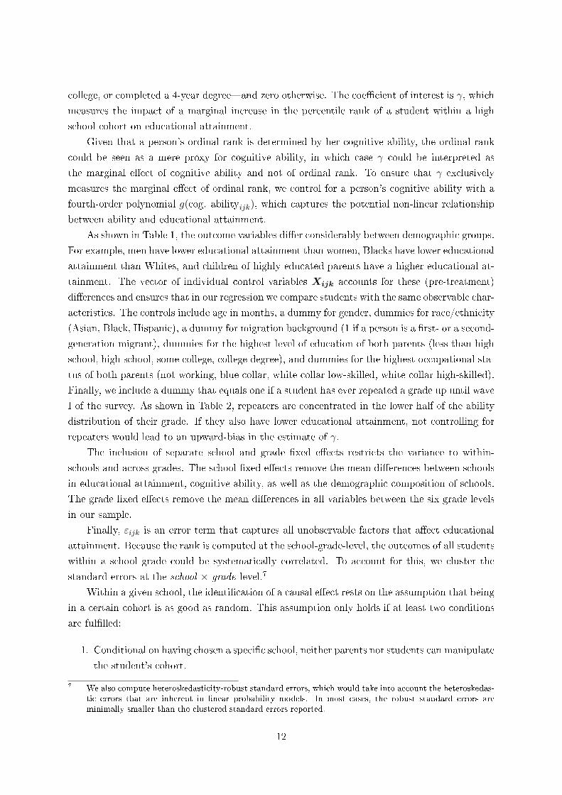
Given that a person's ordinal rank is determined by her cognitive ability, the ordinal rank
could be seen as a mere proxy for cognitive ability, in which case γ could be interpreted as
the marginal e�ect of cognitive ability and not of ordinal rank. To ensure that γ exclusively
measures the marginal e�ect of ordinal rank, we control for a person's cognitive ability with a
fourth-order polynomial g(cog. abilityijk), which captures the potential non-linear relationship
between ability and educational attainment.
As shown in Table 1, the outcome variables di�er considerably between demographic groups.
For example, men have lower educational attainment than women, Blacks have lower educational
attainment than Whites, and children of highly educated parents have a higher educational at-
tainment. The vector of individual control variables Xijk accounts for these (pre-treatment)
di�erences and ensures that in our regression we compare students with the same observable char-
acteristics. The controls include age in months, a dummy for gender, dummies for race/ethnicity
(Asian, Black, Hispanic), a dummy for migration background (1 if a person is a �rst- or a second-
generation migrant), dummies for the highest level of education of both parents (less than high
school, high school, some college, college degree), and dummies for the highest occupational sta-
tus of both parents (not working, blue collar, white collar low-skilled, white collar high-skilled).
Finally, we include a dummy that equals one if a student has ever repeated a grade up until wave
I of the survey. As shown in Table 2, repeaters are concentrated in the lower half of the ability
distribution of their grade. If they also have lower educational attainment, not controlling for
repeaters would lead to an upward-bias in the estimate of γ.
The inclusion of separate school and grade �xed e�ects restricts the variance to within-
schools and across-grades. The school �xed e�ects remove the mean di�erences between schools
in educational attainment, cognitive ability, as well as the demographic composition of schools.
The grade �xed e�ects remove the mean di�erences in all variables between the six grade levels
in our sample.
Finally, εijk is an error term that captures all unobservable factors that a�ect educational
attainment. Because the rank is computed at the school-grade-level, the outcomes of all students
within a school grade could be systematically correlated. To account for this, we cluster the
standard errors at the school × grade-level.7
Within a given school, the identi�cation of a causal e�ect rests on the assumption that being
in a certain cohort is as good as random. This assumption only holds if at least two conditions
are ful�lled:
1. Conditional on having chosen a speci�c school, neither parents nor students can manipulate
the student's cohort.
7 We also compute heteroskedasticity-robust standard errors, which would take into account the heteroskedas-tic errors that are inherent in linear probability models. In most cases, the robust standard errors areminimally smaller than the clustered standard errors reported.
12
2. Within a school, there is no systematic correlation between average cohort characteristics
and educational attainment.
Violations to any of these conditions could introduce a systematic bias into the estimate
of γ, as the ordinal rank would be correlated with the error term, cov(ordinal rankijk, εijk) 6=0. Potential violations to the �rst condition could be due to strategic delay of school entry
(redshirting) or grade repetition. Examples for violations of the second condition are changes
in the cohort quality within a school, or a direct e�ect of the average peer quality on outcomes.
For the baseline analysis to follow, we maintain the assumption that both conditions hold.
In robustness checks, we will address a large number of confounding factors, and also discuss
measurement error and selective attrition as potential sources of bias.
4 Results
In this section, we present the estimation results. We begin by exploring the unconditional
relationship between rank and three measures of educational attainment; we then gradually
introduce �xed e�ects and control variables into the model. We further explore whether the
e�ect di�ers between school types and whether it is non-linear within a cohort. While the
baseline model rules out some obvious confounders, the results could still be biased due to
omitted factors, measurement error, or attrition. In a series of robustness checks, we show that
that these biases do not lead to dramatic changes in the results. Finally, we explore potential
channels through which a student's rank a�ects educational attainment.
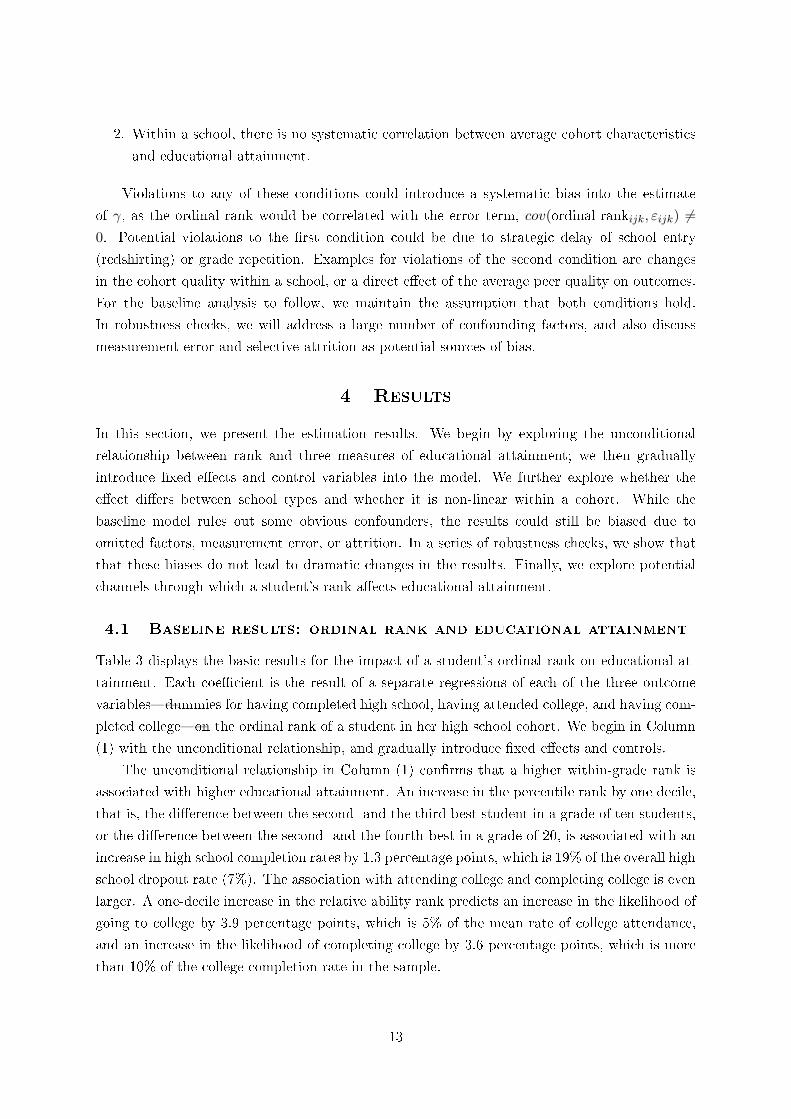
4.1 Baseline results: ordinal rank and educational attainment
Table 3 displays the basic results for the impact of a student's ordinal rank on educational at-
tainment. Each coe�cient is the result of a separate regressions of each of the three outcome
variables�dummies for having completed high school, having attended college, and having com-
pleted college�on the ordinal rank of a student in her high school cohort. We begin in Column
(1) with the unconditional relationship, and gradually introduce �xed e�ects and controls.
The unconditional relationship in Column (1) con�rms that a higher within-grade rank is
associated with higher educational attainment. An increase in the percentile rank by one decile,
that is, the di�erence between the second- and the third-best student in a grade of ten students,
or the di�erence between the second- and the fourth-best in a grade of 20, is associated with an
increase in high school completion rates by 1.3 percentage points, which is 19% of the overall high
school dropout rate (7%). The association with attending college and completing college is even
larger. A one-decile increase in the relative ability rank predicts an increase in the likelihood of
going to college by 3.9 percentage points, which is 5% of the mean rate of college attendance,
and an increase in the likelihood of completing college by 3.6 percentage points, which is more
than 10% of the college completion rate in the sample.
13
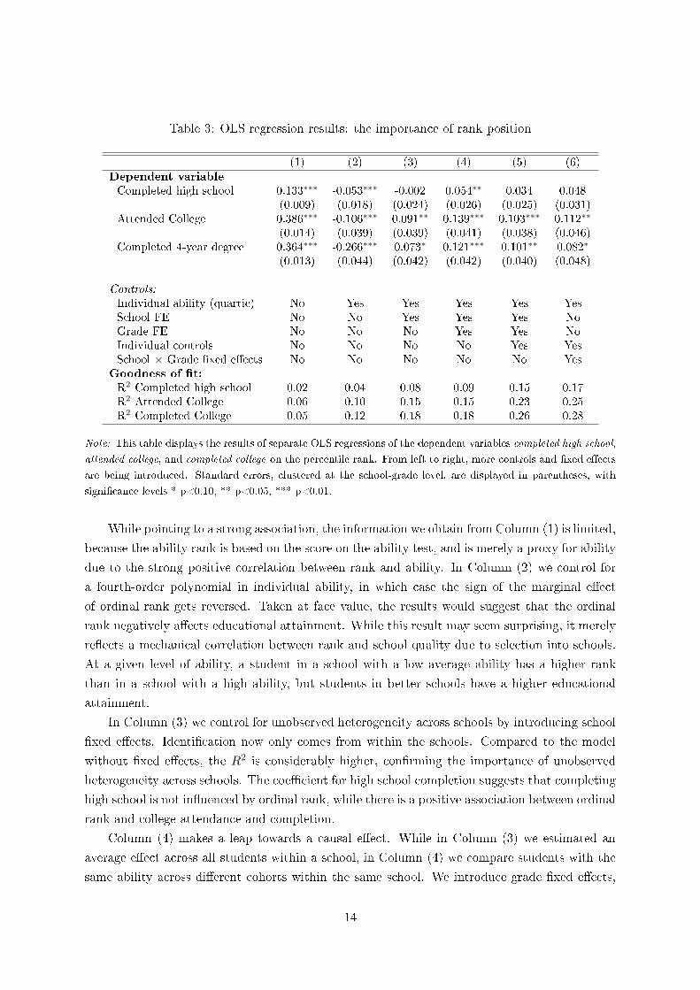
Table 3: OLS regression results: the importance of rank position
(1) (2) (3) (4) (5) (6)
Dependent variable
Completed high school 0.133∗∗∗ -0.053∗∗∗ -0.002 0.054∗∗ 0.034 0.048(0.009) (0.018) (0.024) (0.026) (0.025) (0.031)
Attended College 0.386∗∗∗ -0.106∗∗∗ 0.091∗∗ 0.139∗∗∗ 0.103∗∗∗ 0.112∗∗
(0.014) (0.039) (0.039) (0.041) (0.038) (0.046)Completed 4-year degree 0.364∗∗∗ -0.266∗∗∗ 0.073∗ 0.121∗∗∗ 0.101∗∗ 0.082∗
(0.013) (0.044) (0.042) (0.042) (0.040) (0.048)
Controls:Individual ability (quartic) No Yes Yes Yes Yes YesSchool FE No No Yes Yes Yes NoGrade FE No No No Yes Yes NoIndividual controls No No No No Yes YesSchool × Grade �xed e�ects No No No No No Yes
Goodness of �t:
R2 Completed high school 0.02 0.04 0.08 0.09 0.15 0.17R2 Attended College 0.06 0.10 0.15 0.15 0.23 0.25R2 Completed College 0.05 0.12 0.18 0.18 0.26 0.28
Note: This table displays the results of separate OLS regressions of the dependent variables completed high school,
attended college, and completed college on the percentile rank. From left to right, more controls and �xed e�ects
are being introduced. Standard errors, clustered at the school-grade level, are displayed in parentheses, with
signi�cance levels * p<0.10, ** p<0.05, *** p<0.01.
While pointing to a strong association, the information we obtain from Column (1) is limited,
because the ability rank is based on the score on the ability test, and is merely a proxy for ability
due to the strong positive correlation between rank and ability. In Column (2) we control for
a fourth-order polynomial in individual ability, in which case the sign of the marginal e�ect
of ordinal rank gets reversed. Taken at face value, the results would suggest that the ordinal
rank negatively a�ects educational attainment. While this result may seem surprising, it merely
re�ects a mechanical correlation between rank and school quality due to selection into schools.
At a given level of ability, a student in a school with a low average ability has a higher rank
than in a school with a high ability, but students in better schools have a higher educational
attainment.
In Column (3) we control for unobserved heterogeneity across schools by introducing school
�xed e�ects. Identi�cation now only comes from within the schools. Compared to the model
without �xed e�ects, the R2 is considerably higher, con�rming the importance of unobserved
heterogeneity across schools. The coe�cient for high school completion suggests that completing
high school is not in�uenced by ordinal rank, while there is a positive association between ordinal
rank and college attendance and completion.
Column (4) makes a leap towards a causal e�ect. While in Column (3) we estimated an
average e�ect across all students within a school, in Column (4) we compare students with the
same ability across di�erent cohorts within the same school. We introduce grade �xed e�ects,
14
which absorb the mean di�erence between di�erent cohorts across the sample. If students who
were in 7th grade in 1994 were, on average, di�erent from those in 8th grade, this di�erence is
accounted for in this speci�cation. Compared to Column (3), the e�ects are larger and more
precisely estimated. For all three outcome variables, these e�ects are substantial. An increase
in the within-grade rank by one decile increases the likelihood of completing high school by half
a percentage point, and increases college attendance and completion by 1.4 and 1.2 percentage
points (2% and 3.6% of the mean), respectively.
In Column (5) we introduce individual control variables to take into account the di�erences
in observable characteristics, and their potential e�ect on the outcome. There are two reasons for
including control variables. First, as shown in Table 1, the outcome variables di�er signi�cantly
across ethnic and parental backgrounds. Second, as indicated by the increased R2 in Column
(5), the control variables have additional explanatory power and ensure a better model �t. The
inclusion of individual controls, however, has no statistically signi�cant impact on the point
estimates, which lends further credibility to our claim that cross-cohort variation in the ability
distribution within the same school is quasi-random. The point estimates in Column (5) are
slightly smaller than in Column (4), but the di�erence is not statistically signi�cant.
Finally, we address the concern that the average grade characteristics, for example, average
peer ability, bias the estimates. In Column (6) we include school × grade �xed e�ects, taking
into account school-speci�c mean di�erences across grades. The only variation exploited by this
speci�cation is in the variance of the ability distribution within schools across grades. Some
cohorts have a more dispersed ability distribution than others, such that a given level of ability
leads to a di�erent rank when the variances are di�erent but the mean is the same. It is reassuring
that the results from this demanding speci�cation are similar to those in the estimation with
separate sets of �xed e�ects in Column (5). The di�erences between the coe�cients in Columns
(5) and (6) are not statistically signi�cant. Moreover, the results in Column (6) indicate that
the variation in rank is mainly driven by the di�erences in variance, rather than di�erences in
the mean ability.
In sum, these results clearly show that a student's rank matters for educational choices and
outcomes. We �nd large and statistically signi�cant di�erences in high-school completion rates,
college attendance, and college completion of students who go to the same school but have a
di�erent rank in the ability distribution of their grade.
4.2 Heterogeneous effects
While the regression results in Table 3 show a positive impact of high school rank position on
educational attainment, the strength of this impact di�ers along the ranking and across school
types. The �rst three rows in Figure 2 displays the results for di�erent school types, which we
obtained by re-estimating Equation 3 on split samples. The three classi�cations are given in the
survey and are the only available measure of school size. As shown in the �rst row, the e�ects
di�er considerably by school size. For college attendance and completion, the e�ects are mainly
driven by large and medium-sized schools, while the e�ect for high-school completion is larger
15
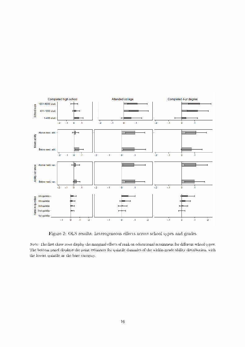
Figure 2: OLS results: heterogeneous e�ects across school types and grades
Note: The �rst three rows display the marginal e�ects of rank on educational attainment for di�erent school types.
The bottom panel displays the point estimates for quintile dummies of the within-grade ability distribution, with
the lowest quintile as the base category.
16
in smaller schools. The larger e�ects in larger schools is evidence against measurement error in
the rank variable, which could be due to strati�ed random sampling. Because a �xed number
of students was sampled from a grade regardless of the grade size, we would expect a greater
measurement error and, consequently, a greater attenuation bias in larger schools.
We also test whether the e�ects are di�erent in high- and low-ability schools, as well as in
more and less heterogeneous schools. The second row of Figure 2 displays separate e�ects for
schools with an average ability above and below the median: the e�ect is the same regardless of
whether the school has a high or a low average ability. Similarly, we consider schools with a high
and low variance in ability. In segregated neighborhoods, we would expect a greater homogeneity
within schools, and the ordinal rank could be more important in more or less segregated schools.
However, we �nd no di�erence in the e�ect between high- and low-variance schools.
Finally, we consider non-linear e�ects within a grade. According to the linear e�ect in Table
3, going from rank 60 to rank 50 in a cohort of 100 would make the same di�erence as going
from rank 10 to rank 1. This can hardly be the case. While we lack the statistical power to test
for non-linearities along the entire ranking, we provide evidence for a non-linear e�ect based on
quintiles of the within-grade ability distribution. We estimate a model similar to Equation (3)
but replace the percentile rank with dummy variables for the quintiles 2-5. The lowest quintile
is the base category. As shown in the fourth row of Figure 2, the e�ect is virtually zero in
the bottom half of the within-grade distribution. From the third quintile onwards, the e�ect is
positive, and the relationship between rank and educational outcomes looks linear.
4.3 Discussion and robustness checks
Thus far, we have interpreted the rank e�ect on educational attainment as causal, given that
the individual controls as well as the �xed e�ects rule out many confounding factors, and based
on the assumption that being in one school cohort or another is exogenous to the student. In
this section, we discuss various sources of bias and demonstrate that the results are robust to
numerous speci�cation checks. Table 4 displays the results. The baseline results in row 1) serve
as a benchmark.
Does the rank measure reflect non-cognitive skills? One concern with the
Peabody test score as a measure for cognitive ability is that it could in part re�ect personality
traits. Peabody is not a high-stakes test, and students had no particular incentive to achieve a
high test score. Therefore, one would expect more conscientious students to put more e�ort into
the test and achieve a higher score. Exploiting information on conscientiousness and neuroticism
in the �rst wave of AddHealth, we carry out two tests to assess whether our rank measure,
in part, re�ects non-cognitive skills. We �rst regress the percentile rank on both personality
measures, controlling for individual characteristics, as well as school and grade �xed e�ects. If the
rank measure re�ected non-cognitive skills, we would expect statistically signi�cant coe�cients
for both non-cognitive skills. As shown in Appendix B, the coe�cients are close to zero and
statistically insigni�cant. In Row 2) of Table 4, we also include both measures as endogenous
17
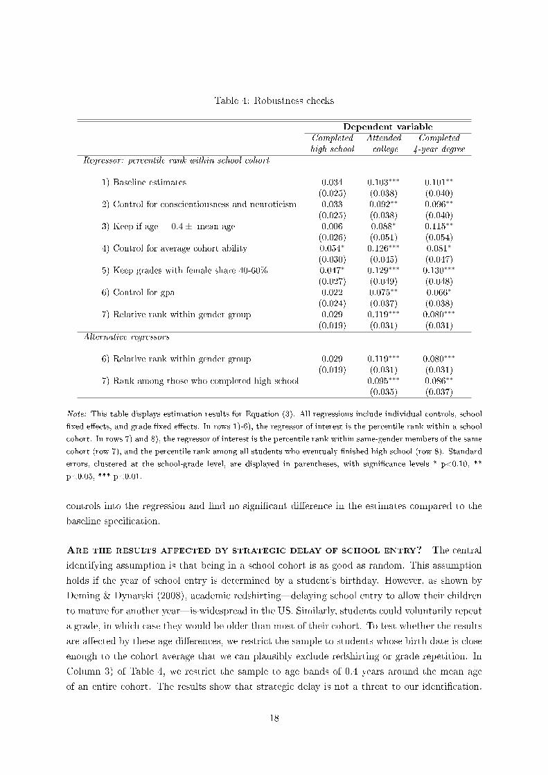
Table 4: Robustness checks
Dependent variable
Completed Attended Completedhigh school college 4-year degree
Regressor: percentile rank within school cohort
1) Baseline estimates 0.034 0.103∗∗∗ 0.101∗∗
(0.025) (0.038) (0.040)2) Control for conscientiousness and neuroticism 0.033 0.092∗∗ 0.096∗∗
(0.025) (0.038) (0.040)3) Keep if age = 0.4± mean age 0.006 0.088∗ 0.115∗∗
(0.026) (0.051) (0.054)4) Control for average cohort ability 0.054∗ 0.126∗∗∗ 0.081∗
(0.030) (0.045) (0.047)5) Keep grades with female share 40-60% 0.047∗ 0.129∗∗∗ 0.130∗∗∗
(0.027) (0.049) (0.048)6) Control for gpa 0.022 0.075∗∗ 0.066∗
(0.024) (0.037) (0.038)7) Relative rank within gender group 0.029 0.119∗∗∗ 0.080∗∗∗
(0.019) (0.031) (0.031)
Alternative regressors
6) Relative rank within gender group 0.029 0.119∗∗∗ 0.080∗∗∗
(0.019) (0.031) (0.031)7) Rank among those who completed high-school 0.095∗∗∗ 0.086∗∗
(0.035) (0.037)
Note: This table displays estimation results for Equation (3). All regressions include individual controls, school
�xed e�ects, and grade �xed e�ects. In rows 1)-6), the regressor of interest is the percentile rank within a school
cohort. In rows 7) and 8), the regressor of interest is the percentile rank within same-gender members of the same
cohort (row 7), and the percentile rank among all students who eventualy �nished high school (row 8). Standard
errors, clustered at the school-grade level, are displayed in parentheses, with signi�cance levels * p<0.10, **
p<0.05, *** p<0.01.
controls into the regression and �nd no signi�cant di�erence in the estimates compared to the
baseline speci�cation.
Are the results affected by strategic delay of school entry? The central
identifying assumption is that being in a school cohort is as good as random. This assumption
holds if the year of school entry is determined by a student's birthday. However, as shown by
Deming & Dynarski (2008), academic redshirting�delaying school entry to allow their children
to mature for another year�is widespread in the US. Similarly, students could voluntarily repeat
a grade, in which case they would be older than most of their cohort. To test whether the results
are a�ected by these age di�erences, we restrict the sample to students whose birth date is close
enough to the cohort average that we can plausibly exclude redshirting or grade repetition. In
Column 3) of Table 4, we restrict the sample to age bands of 0.4 years around the mean age
of an entire cohort. The results show that strategic delay is not a threat to our identi�cation.
18
The e�ect on high school completion is now zero, but the e�ects on college attendance and
completion are close to the baseline estimates.
Are the baseline results affected by average peer quality? Much of the
peer e�ects literature shows that the average peer ability has a positive impact on individual
student outcomes (Sacerdote, 2011). In our baseline model, average peer ability�and in fact any
other school-grade-speci�c characteristic�would be an omitted variable, and bias the estimate
of γ. By using a more demanding speci�cation with school × grade �xed e�ects, we were able to
net out all confounders at the grade-level within a school, and we have shown in Column 6) of
Table 3 that this approach yields very similar results. However, including school × grade �xed
e�ects takes out a great deal of variation, and identi�es the e�ect only from the di�erences in
the ability variance across cohorts within a school. In Table 4 Row 4), we present the results of
a more straightforward speci�cation, in which we include average peer ability as an additional
control in the baseline model. The results are similar to those from a model with school × grade
�xed e�ects as well as the baseline model. The estimate for college attendance is higher than in
the other models, but the di�erence in coe�cients is not statistically signi�cant.
Are same-gender peers more important? We were also interested whether all stu-
dents in the same grade are the relevant comparison group or whether students with the same
gender are more important. It may matter more if a girl is the best among all girls, rather
than being the best among everyone in the grade. In Row 7) of Table 4, we replace the ordinal
rank in a school grade with the ordinal rank within a gender group within a grade. The results
are almost identical as in the baseline speci�cation, indicating that same-gender peers are as
important as all students in the same cohort.
Measurement error A potential source of bias is measurement error in the ordinal rank.
One source of measurement error could be the over-sampling of minorities. If minority students
have a lower average ability compared to white Americans in their grade, and if they are over-
sampled, then white Americans would be assigned a higher ordinal rank than under random
sampling. The sequencing of the sampling in AddHealth o�ers an opportunity to assess the size
of the measurement error. First, a random sample was drawn and labeled as the core sample,
and second, additional students were drawn from given minorities. Hence, we observe for each
student in the sample the rank with and without over-sampling. The correlation in the percentile
ranks in both samples is 0.9867, indicating that measurement error from over-sampling is not a
concern.
A further source of measurement error is gender strati�cation. Within each school grade,
equal numbers of boys and girls were drawn, unless the school is a single-sex school. This
sampling could introduce measurement error in the rank measure if the population gender dis-
tribution within a grade is skewed. Consider a grade of 100 students, of which 20 are female. If
we draw 17 male and 17 female students, then we would sample 85% of all females, but only 21%
19
of all males in a grade. To assess the extent to which strati�ed sampling a�ects the estimates,
we exclude grades in which the share of girls is greater than 60
Finally, measurement error could arise from the random sampling of students within grades.
In most schools, around 25% of all students in a school grade were drawn at random. The
random sampling introduces a standard measurement error, which may lead to a downward bias
in the results. The heterogeneous e�ects in Figure 2 give us some idea about the magnitude
of this bias. Given that the same number of students is drawn regardless of the grade size, we
would expect a larger measurement error and smaller estimates in larger schools. While this is
not a de�nitive proof, the evidence goes against a large measurement error, given that we �nd
smaller e�ects in smaller schools.
Selective attrition An additional source of bias is selective attrition. We are not able
to track all students from wave I to wave IV; around 25% of all students attrit from the sample.
This attrition may lead to biased estimates if it is correlated with the rank. We address this
concern in a robustness check in Appendix B, in which we estimate Equation 3 with the attrition
status as the dependent variable, and �nd no evidence for a systematic relationship between rank
and attrition.
An additional source of attrition may have occurred before and up to wave I: high-school
dropouts. Because we observe each cohort in a di�erent grade, high-school dropouts should
induce a greater attrition in older compared to younger cohorts. To the extent that dropouts
predominantly come from the low end of the within-cohort ability distribution, the ability dis-
tribution may shift to the right over time. These shifts should not a�ect our results, because
the average shifts would be absorbed by the grade �xed e�ects, and school-cohort-speci�c shifts
would be absorbed by the school-speci�c grade �xed e�ects. Nevertheless, we carry out a ro-
bustness check that demonstrates that this dynamic attrition is not an issue. We recalculate the
rank measure using only students in wave I who have indicated in wave IV that they completed
high school. The results, displayed in row 8) for the two college outcomes, are stable to the use
of this alternative rank measure.
Ability vs. gpa We chose cognitive ability, measured by a standardized ability test, as a
base for the rank measure mainly because a standardized test allows us to compare students
across cohorts within a school. A further possibility would be to rank students according to their
grade point average (GPA), which is a more salient measure. At the same time, GPA is not
standardized, and thus not comparable across cohorts; it is self-reported, and has a great deal of
missing information. One might be concerned, however, that the ability rank is merely a proxy
for a rank based on academic performance. In Row 6) of of Table 4, we assess the importance
of GPA in explaining the results, by including it as an additional endogenous regressor. If the
ability rank was merely re�ecting GPA, then its coe�cient should be small and statistically
insigni�cant. As shown in Row 6) of of Table 4, including GPA reduces the coe�cients by
around one third, but they remain statistically and economically signi�cant. Rather than being
20
a competing measure for ability, grades can be seen as one channel through which a student's
relative ability a�ects outcomes.
4.4 Potential channels
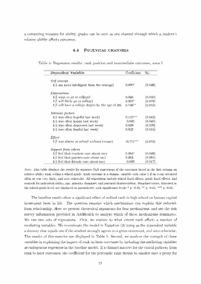
Table 5: Regression results: rank position and intermediate outcomes, wave I
Dependent Variable Coe�cient SE
Self-concept1(I am more intelligent than the average) 0.090∗ (0.046)
Expectations1(I want to go to college) 0.028 (0.040)1(I will likely go to college) 0.082∗ (0.042)1(I will have a college degree by the age of 30) 0.106∗∗ (0.043)
Intrinsic factors1(I was often hopeful last week) 0.110∗∗∗ (0.042)1(I was often happy last week) -0.002 (0.040)1(I was often depressed last week) 0.029 (0.029)1(I was often fearful last week) 0.022 (0.018)
E�ort1(I was absent at school without excuse) -0.115∗∗∗ (0.043)
Support from others1(I feel that teachers care about me) 0.085∗ (0.049)1(I feel that parents care about me) 0.003 (0.031)1(I feel that friends care about me) -0.003 (0.017)
Note: This table displays the results for separate OLS regressions of the outcomes listed in the �rst column on
relative ability rank within a school grade. Each outcome is a dummy variable with value 1 if an event occurred
often or was very likely, and zero otherwise. All regressions include school �xed e�ects, grade �xed e�ects, and
controls for individual ability, age, minority dummies, and parental characteristics. Standard errors, clustered at
the school-grade level, are displayed in parentheses, with signi�cance levels * p<0.10, ** p<0.05, *** p<0.01.
The baseline results show a signi�cant e�ect of ordinal rank in high school on human capital
investment later in life. The question remains which mechanisms can explain this reduced-
form relationship. Here we present theoretical arguments for four mechanisms, and use the rich
survey information provided in AddHealth to analyze which of these mechanisms dominates.
We run two sets of regressions. First, we explore to what extent rank a�ects a number of
mediating variables. We re-estimate the model in Equation (3) using as the dependent variable
a dummy that equals one if the student strongly agrees to a given statement, and zero otherwise.
The results of this exercise are displayed in Table 5. Second, we analyze the strength of these
variables in explaining the impact of rank on later outcomes by including the mediating variables
as endogenous regressors in the baseline model. If a channel matters for the causal pathway from
rank to later outcomes, the coe�cient for the percentile rank should be smaller once a proxy for
21
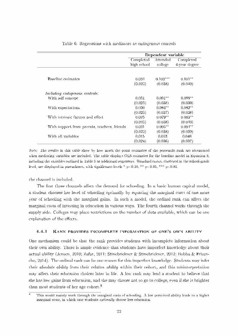
Table 6: Regressions with mediators as endogenous controls
Dependent variable
Completed Attended Completedhigh school college 4-year degree
Baseline estimates 0.034 0.103∗∗∗ 0.101∗∗
(0.025) (0.038) (0.040)
Including endogenous controls:With self-concept 0.031 0.091∗∗ 0.089∗∗
(0.025) (0.038) (0.039)With expectations 0.030 0.084∗∗ 0.082∗∗
(0.025) (0.037) (0.038)With intrinsic factors and e�ort 0.025 0.079∗∗ 0.083∗∗
(0.025) (0.038) (0.040)With support from parents, teachers, friends 0.031 0.095∗∗ 0.094∗∗
(0.025) (0.038) (0.039)With all variables 0.015 0.053 0.048
(0.024) (0.036) (0.037)
Note: The results in this table show by how much the point estimates of the percentile rank are attenuated
when mediating variables are included. The table displays OLS estimates for the baseline model in Equation 3,
including the variables outlined in Table 5 as additional regressors. Standard errors, clustered at the school-grade
level, are displayed in parentheses, with signi�cance levels * p<0.10, ** p<0.05, *** p<0.01.
the channel is included.
The �rst three channels a�ect the demand for schooling. In a basic human capital model,
a student chooses her level of schooling optimally by equating the marginal costs of one more
year of schooling with the marginal gains. In such a model, the ordinal rank can a�ect the
marginal costs of investing in education in various ways. The fourth channel works through the
supply side. Colleges may place restrictions on the number of slots available, which can be one
explanation of the e�ects.
4.4.1 Rank provides incomplete information of one's own ability
One mechanism could be that the rank provides students with incomplete information about
their own ability. There is ample evidence that students have imperfect knowledge about their
actual ability (Jensen, 2010; Zafar, 2011; Stinebrickner & Stinebrickner, 2012; Bobba & Frisan-
cho, 2014). The ordinal rank can be one reason for this imperfect knowledge. Students may infer
their absolute ability from their relative ability within their cohort, and this misinterpretation
may a�ect their education choices later in life. A low rank may lead a student to believe that
she has low gains from education, and she may choose not to go to college, even if she is brighter
than most students of her age cohort.8
8 This would mainly work through the marginal costs of schooling. A low perceived ability leads to a highermarginal costs, in which case students optimally choose less education.
22
Here we provide evidence that the ordinal rank a�ects perceived ability and expectations.
We �rst assess whether students with a higher rank have a higher perceived ability�a frequent
�nding in the psychology literature (Marsh, 1987). As shown in the �rst panel of Table 5, this is
indeed the case. In wave I of AddHealth, students were asked if they think that they are more
intelligent than the average. Conditional on absolute ability, students with a 10 percentage
points higher rank are 0.9 percentage points more likely to believe that they are more intelligent
than the average. Table 5 shows that self-concept can explain part of the overall e�ect of rank
on later outcomes. The coe�cients for the college variables are around 10 percent lower once
perceived ability is included.
Furthermore, we proxy for expected returns to education with various measures of career
expectations. In wave I, students were asked whether they want to go to college, whether they
will likely go to college, and whether they expect to have a college degree at the age of 30. We
�nd strong support that rank a�ects expected returns to education. As shown in the second
panel of Table 5, students with a higher rank are more likely to state that they will go to college,
and they are more likely to think that they will have a college degree by age 30. Remarkably,
the impact of rank on college expectations at age 16 is equally as large as the impact of rank
on actual college outcomes more than 10 years later. Also, as shown in Table 6, including
expectations attenuates the baseline estimate by around 20%, showing that the expectations
channel is quantitatively important.
Intrinsic factors and effort The e�ect could also be explained by intrinsic factors.
As suggested by the literature on relative comparisons and e�ort provision, a higher rank may
give students a greater motivation, make them more self-con�dent, and ultimately induce them
to exert more e�ort in their studies (Clark et al., 2010; Azmat & Iriberri, 2010). E�ort, in turn,
would increase the marginal gains from schooling, and induce students to choose more schooling.
The third panel in Table 5 displays the impact of ordinal rank on intrinsic factors, exploiting
questions from a survey module on mental distress. Students with a higher rank are signi�cantly
more optimistic, while we �nd no e�ect of rank on happiness, depression, or fearfulness. To
proxy for e�ort, we use self-reported information on school absences, and construct a dummy
that equals one if the student has been absent without excuse at least once in the previous school
year. We �nd that students with a higher rank are signi�cantly less likely to be absent without
excuse, which indicates that they take their studies more seriously and put more e�ort into it.
In Table 6 we include the intrinsic factors and the absence dummy into the baseline regression.
These factors explain as much of the e�ect of rank on educational attainment as the inclusion
of expectations. The coe�cients are around 20% smaller.
Behavioral responses from teachers, parents, and friends A further poten-
tial channel is behavioral responses from a student's environment. As shown by Pop-Eleches &
Urquiola (2013), teachers and parents are responsive to a student's relative position within their
school. They compare marginal students who just made it into a high-quality school to those
23
who did not and �nd that parents provide less e�ort when their child attends a better school.
Moreover, teachers could have a preference for students with a higher rank and give them more
support. More support from the environment lowers the marginal costs of schooling, and�all
else equal�should lead to more schooling.
In the �fth panel of Table 5, we show the e�ect of percentile rank on perceived support
from teachers, parents, and friends. Students were asked whether they believe that these groups
care about them. The ordinal rank has indeed a positive impact on the perceived support from
teachers. Students with a higher rank are more likely to feel that their teachers care about
them. The e�ects on the perceived support from parents and friends, in contrast, are small
and statistically insigni�cant. When we include the support variables into the main regression,
the coe�cient of the percentile rank does not decrease by a large amount, indicating that the
support from the environment plays a minor role in explaining the result.
Selective college admissions Finally, the e�ect can be explained by college admissions.
Colleges may have a �xed number of slots and/or a �xed amount of �nancial aid available and
may give priority to students with a higher within-school rank. In light of the channels we
analyzed so far, college admissions, if anything, can only explain part of the e�ect. We have
shown that rank a�ects a student's perceived ability, ambition, e�ort, and expectations before
students apply for colleges. If supply side restrictions were the only explanations for the e�ect,
then we should not see a signi�cant e�ect of rank on these other outcomes. Moreover, the
outcome variable attended college includes all colleges in the US, that is, it also includes a vast
number of non-selective community colleges for which these restrictions typically do not apply.
If restrictions were the only explanation, we would expect to �nd no e�ect on attending any
college.
A further supply-side channel is a�rmative action, through which colleges may give preferen-
tial access to students from minorities or from schools in disadvantaged areas. While a�rmative
action has been shown to signi�cantly distort sorting into colleges (Arcidiacono, 2005), it should
not explain our results, because we control for many characteristics that de�ne the minori-
ties targeted by a�rmative action, such as Blacks or Hispanics. However, following prominent
lawsuits in the mid-1990s, many state colleges in the US have abandoned a�rmative action.
Instead, California, Texas, and Florida introduced ten-percent plans, granting students in the
top 10 percent of their high school cohort automatic access to �agship state universities.9 These
10%-plans were introduced three years after the �rst wave of AddHealth was collected and, thus,
should only a�ect the youngest cohorts, if at all.
Besides these plans that speci�cally apply to students with a given rank, the e�ect of rank
on college outcomes can more generally be explained by selective college admission policies. Stu-
9 Daugherty et al. (2014) for Texas and Arcidiacono et al. (2014) for California give evidence that the intro-duction of these plans changed the composition of students at �agship state colleges. In Texas, attendanceand completion rates at these colleges increased, but more so for students from high-ability high schools. InCalifornia the college attendance rates of Blacks increased, but larger shares of Blacks went to lower-rankedcolleges.
24
dents typically apply for college with their 11th-grade results, which often state the percentile of
a student in the GPA distribution of her grade. If college admission o�cers have this informa-
tion, and if GPA rank is positively correlated with the ability rank, then our result could re�ect
a pure mechanical e�ect: colleges only admit students with a higher rank, which is why we
observe higher college attendance rates for highly ranked students. While we do not have direct
information on the type of college to which students apply or are admitted, we have shown in
Table 4 that GPA can only explain a small fraction of the e�ect of rank on college attendance.
Hence, college admissions can�if at all�only in part explain the results.
5 Conclusion
In this paper we show that a student's ordinal rank in a high school cohort is an important
determinant for educational attainment later in life. Comparing students across cohorts within
the same school, and �exibly controlling for cognitive ability, we �nd that students with a higher
ordinal rank in their cohort are more likely to complete high school, attend college, and complete
a 4-year degree. This e�ect runs counter to most of the literature on peer e�ects, which �nds
that being exposed to better peers has a positive e�ect on educational attainment.
Exploiting rich survey information, we provide evidence on the mechanisms that help to
explain this result. We �nd that students with a higher rank have higher expectations about
their future career outcomes, they are more optimistic and more self-con�dent, and they receive
more attention from their teachers. These results suggest that students base their schooling
decisions in part on their relative rather than their absolute ability. The ordinal rank provides
students with noisy information about their own ability, which in turn distorts the trade-o�
between the short-run costs and the long-run bene�ts from schooling.
Our results should concern parents and policymakers alike. A student's relative position in a
cohort a�ects outcomes later in life, and parents should take the rank of their child into account
when choosing the right school for their child. The highest-ranked school may not be bene�cial
for children at the margin who only just make it into the school. However, it is also important
to note that rank is only one aspect of school choice. Our results re�ect local e�ects, which we
obtained by comparing students within the same school but in di�erent cohorts. If parents chose
schools exclusively based on their child's rank, they would ignore many other school inputs that
are equally important, such as teacher quality, average peer ability, and school resources.
Policymakers should be concerned, because our results show that students with a high
ability but a low rank�small �sh in a big pond�under-invest in their human capital. Students
seemingly place too much weight on their relative ability and too little on their absolute ability
when making college decisions. It is di�cult to think of an algorithm that reduces this ine�ciency
by regrouping students into schools, because the ordinal rank is a relative measure, and improving
one student's rank means worsening the rank of another. A more e�cient policy could be to
give more support to students at lower ranks of the ability distribution in order to compensate
for the negative impact of their rank. Especially for students with a low rank in high-ability
25
schools, providing them with information on their absolute ability could be an inexpensive and
e�ective way to increase their educational attainment. Recent experimental studies by Azmat &
Iriberri (2010), Tran & Zeckhauser (2012), Hastings & Weinstein (2008), Bettinger et al. (2012),
Oreopoulos & Dunn (2013) and Wiswall & Zafar (2015) have shown that students are indeed
responsive to these type of interventions.
26
References
Abdulkadiroglu, Atila, Angrist, Joshua D., & Pathak, Parag A. 2014. The Elite
Illusion: Achievement E�ects at Boston and New York Exam Schools. Econometrica, 82(1),
137�196.
Ammermueller, Andreas, & Pischke, Jörn-Steffen. 2009. Peer E�ects in European
Primary Schools: Evidence from the Progress in International Reading Literacy Study. Journal
of Labor Economics, 27(3), 315�348.
Arcidiacono, Peter. 2005. A�rmative Action in Higher Education: How do Admission and
Financial Aid Rules A�ect Future Earnings? Econometrica, 73(5), 1477�1524.
Arcidiacono, Peter, Aucejo, Esteban, Coate, Patrick, & Hotz, V. Joseph. 2014.
A�rmative Action and University Fit: Evidence from Proposition 209. IZA Journal of Labor
Economics, 3:7.
Attanasio, Orazio P., & Kaufmann, Katja M. 2015. Education Choices and Returns to
Schooling: Mothers' and Youths' Subjective Expectations and their Role by Gender. Journal
of Development Economics, 109C, 203�216.
Azmat, Ghazala, & Iriberri, Nagore. 2010. The Importance of Relative Performance
Feedback Information: Evidence from a Natural Experiment using High School Students.
Journal of Public Economics, 94, 435�452.
Bettinger, Eric P., Long, Bridget Terry, Oreopoulos, Philip, & Sanbonmatsu,
Lisa. 2012. The Role of Application Assistance and Information in College Decisions: Results
from the H&R Block FAFSA Experiment. The Quarterly Journal of Economics, 127(3),
1205�242.
Bifulco, Robert, Fletcher, Jason M., & Ross, Stephen L. 2011. The E�ect of Class-
mate Characteristics on Post-Secondary Outcomes: Evidence from the Add Health. American
Economic Journal: Economic Policy, 3, 25�53.
Bobba, Matteo, & Frisancho, Veronica. 2014. Learning About Oneself: The E�ects of
Signaling Academic Ability on School Choice. Inter-American Development Bank, mimeo.
Booij, Adam, Leuven, Edwin, & Oosterbeek, Hessel. 2015. Ability Peer E�ects in
University: Evidence from a Randomized Experiment. IZA Discussion Paper, 8769.
Burke, Mary A., & Sass, Tim A. 2013. Classroom Peer E�ects and Student Achievement.
Journal of Labor Economics, 31(1), 51�82.
Calvó-Armengol, Antoni, Patacchini, Eleonora, & Zenou, Yves. 2009. Peer E�ects
and Social Networks in Education. Review of Economic Studies, 76, 1239�1267.
27
Carrell, Scott E., Fullerton, Richard L., & West, James E. 2009. Does Your Cohort
Matter? Measuring Peer E�ects in College Achievement. Journal of Labor Economics, 27(3),
429�464.
Carrell, Scott E., Sacerdote, Bruce I., & West, James E. 2013. From Natural Varia-
tion to Optimal Policy? The Importance of Endogenous Peer Group Formation. Econometrica,
81(3), 855�882.
Clark, Andrew, Masclet, David, & Villeval, Marie-Claire. 2010. E�ort and Com-
parison Income: Experimental and Survey Evidence. Industrial and Labor Relations Review,
63(3), 407�426.
Cullen, Julie Berry, Long, Mark C., & Reback, Randall. 2013. Jockeying for Posi-
tion: Strategic High School Choice under Texas' Top Ten Percent Plan. Journal of Public
Economics, 97, 32�48.
Daugherty, Lindsay, Martorell, Paco, & McFarlin Jr, Isaac. 2014. Percent Plans,
Automatic Admissions, and College Outcomes. IZA Journal of Labor Economics, 3:10.
De Giorgi, Giacomo, & Pellizzari, Michele. 2014. Understanding Social Interactions:
Evidence from the Classroom. Economic Journal, 124(579), 917�953.
Deming, David, & Dynarski, Susan. 2008. The Lengthening of Childhood. Journal of
Economic Perspectives, 22(3), 71�92.
Dunn, Lloyd M., & Dunn, Leota M. 2007. The Peabody Picture Vocabulary Test. 4th edn.
Bloomington, MN: NCS Pearson, Inc.
Feld, Jan, & Zölitz, Ulf. 2014. On the Nature, Estimation and Channels of Peer E�ects.
University of Gothenburg Working Papers in Economics, 596.
Hanushek, Eric A., Kain, John F., Markman, Jacob M., & Rivkin, Steven G. 2003.
Does Peer Ability A�ect Student Achievement? Journal of Applied Econometrics, 527-544.
Harris, Kathleen Mullan. 2009. The National Longitudinal Study of Adolescent to Adult
Health. doi: 10.3886/ICPSR27021.v9.
Harris, K.M., Halpern, C.T., Whitsel, E., Hussey, J., Tabor, J., Entzel, P., &
Udry, J.R. 2009. The National Longitudinal Study of Adolescent to Adult Health: Research
Design [WWW document]. URL: http://www.cpc.unc.edu/projects/addhealth/design.
Hastings, Justine S., & Weinstein, Jeffrey M. 2008. Information, School Choice, and
Academic Achievement: Evidence from Two Experiments. The Quarterly Journal of Eco-
nomics, 123, 1373�1414.
Hoxby, Caroline. 2000a. The E�ects of Class Size on Student Achievement: New Evidence
from Population Variation. The Quarterly Journal of Economics, 115(4), 1239�1285.
28
Hoxby, Caroline. 2000b. Peer E�ects in the Classroom: Learning from Gender and Race
Variation. NBER Working Paper, 7867.
Imberman, Scott, Kugler, Adriana D., & Sacerdote, Bruce. 2012. Katrina's Children:
Evidence on the Structure of Peer E�ects from Hurricane Evacuees. American Economic
Review, 102(5), 2048�2082.
Jensen, Robert. 2010. The Perceived Returns to Education and the Demand for Schooling.
The Quarterly Journal of Economics, 125(2), 515�548.
Koppensteiner, Martin Foureaux. 2012. Class Assignment and Peer Group E�ects: Evi-
dence from Brazilian Primary Schools. University of Leicester Working Paper, 03.
Lavy, Victor, Silva, Olmo, & Weinhardt, Felix. 2012. The Good, the Bad and the
Average: Evidence on Ability Peer E�ects in Schools. Journal of Labor Economics, 30(2),
367�414.
Marsh, Herbert W. 1987. The big-�sh-little-pond e�ect on academic self-concept. Journal
of Educational Psychology, 79(3), 280.
Marsh, Herbert W., Trautwein, Ulrich, Lüdtke, Oliver, Baumert, Jürgen, &
Köller, Olaf. 2007. The Big-Fish-Little-Pond E�ect: Persistent Negative E�ects of Selec-
tive High Schools on Self-Concept After Graduation. American Educational Research Journal.
Murphy, Richard, & Weinhardt, Felix. 2014. Top of the Class: The Importance of
Ordinal Rank. CESifo Working Paper, 4815.
Oreopoulos, Philip, & Dunn, Ryan. 2013. Information and College Access: Evidence from
a Randomized Field Experiment. Scandinavian Journal of Economics, 115(1), 3�26.
Patacchini, Eleonora, Rainone, Eduardo, & Zenou, Yves. 2012. Student Networks
and Long-Run Educational Outcomes: The Strength of Strong Ties. CEPR Discussion Paper,
9149.
Pop-Eleches, Cristian, & Urquiola, Miguel. 2013. Going to a Better School: E�ects
and Behavioral Responses. American Economic Review, 103(4), 1289�1324.
Sacerdote, Bruce. 2001. Peer E�ects with Random Assignment: Results for Dartmouth
Roommates. The Quarterly Journal of Economics, 116(2), 681�704.
Sacerdote, Bruce. 2011. Peer E�ects in Education: How Might They Work, How Big Are
They, and how much Do We Know thus far? In: Hanushek, Eric A., Machin, Stephen,
& Woessmann, Ludger (eds), Handbook of the Economics of Education, vol. 3. North-
Holland.
Stinebrickner, Todd, & Stinebrickner, Ralph. 2012. Learning about Academic Ability
and the College Drop-out Decision. Journal of Labor Economics, 30(4), 707�748.
29
Stinebrickner, Todd, & Stinebrickner, Ralph. 2014. A Major in Science? Initial Beliefs
and Final Outcomes for College Major and Dropout. Review of Economic Studies, 81(1),
426�472.
Tatsi, Eirini. 2015. Endogenous Social Interaction: Which Peers Matter? Goethe University
Frankfurt, mimeo.
Tincani, Michela. 2015. Heterogeneous Peer E�ects and Rank Concerns: Theory and Evi-
dence. University College London, mimeo.
Tran, Anh, & Zeckhauser, Richard. 2012. Rank as an Inherent Incentive: Evidence from
a Field Experiment. Journal of Public Economics, 96, 645�650.
Wiswall, Matthew, & Zafar, Basit. 2015. Determinants of College Major Choices: Iden-
ti�cation from an Information Experiment. Review of Economic Studies, 82(2), 791�824.
Zafar, Basit. 2011. How do College Students Form Expectations? Journal of Labor Economics,
29(2), 301�348.
Zimmerman, David J. 2003. Peer E�ects in Academic Outcomes: Evidence from a Natural
Experiment. Review of Economics & Statistics, 85(1), 9�32.
30
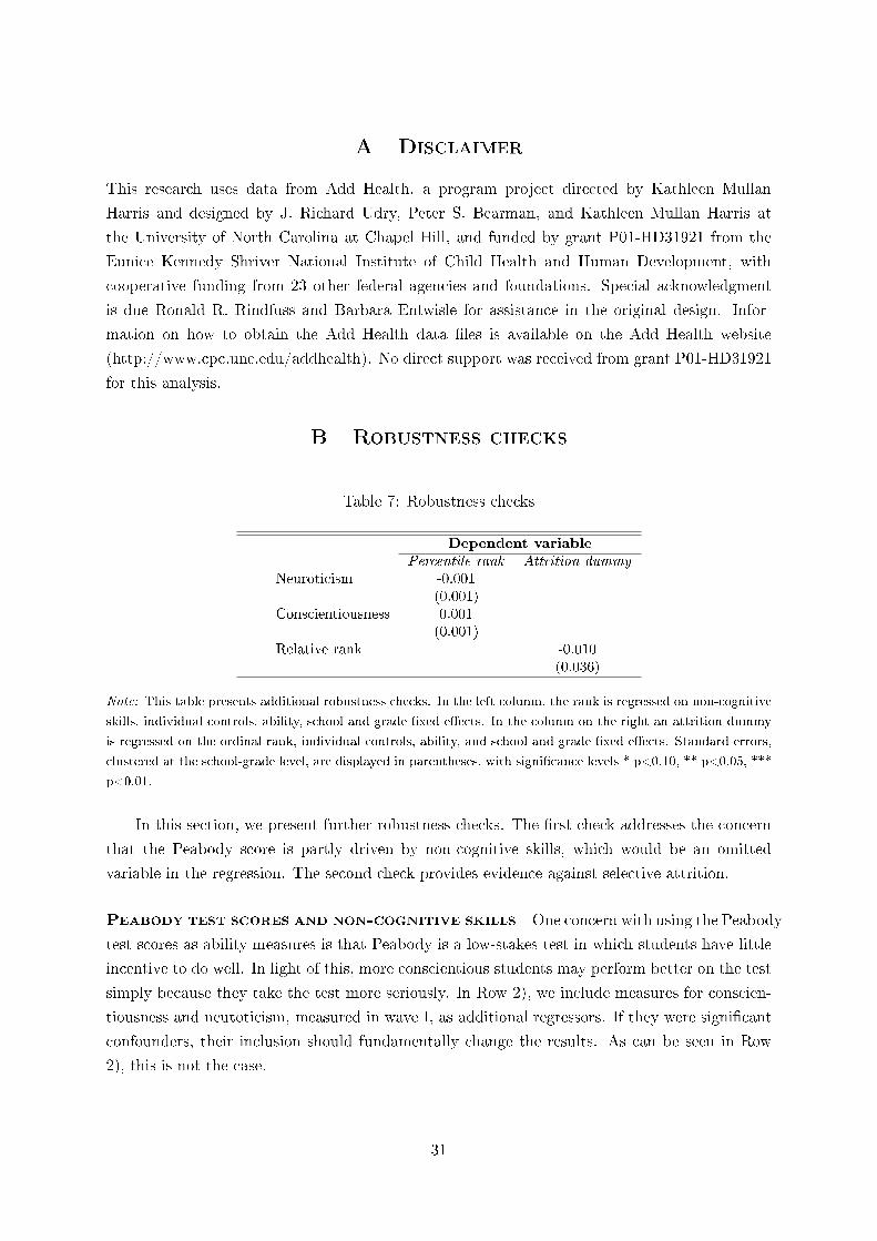
A Disclaimer
This research uses data from Add Health, a program project directed by Kathleen Mullan
Harris and designed by J. Richard Udry, Peter S. Bearman, and Kathleen Mullan Harris at
the University of North Carolina at Chapel Hill, and funded by grant P01-HD31921 from the
Eunice Kennedy Shriver National Institute of Child Health and Human Development, with
cooperative funding from 23 other federal agencies and foundations. Special acknowledgment
is due Ronald R. Rindfuss and Barbara Entwisle for assistance in the original design. Infor-
mation on how to obtain the Add Health data �les is available on the Add Health website
(http://www.cpc.unc.edu/addhealth). No direct support was received from grant P01-HD31921
for this analysis.
B Robustness checks
Table 7: Robustness checks
Dependent variable
Percentile rank Attrition dummyNeuroticism -0.001
(0.001)Conscientiousness 0.001
(0.001)Relative rank -0.010
(0.036)
Note: This table presents additional robustness checks. In the left column, the rank is regressed on non-cognitive
skills, individual controls, ability, school and grade �xed e�ects. In the column on the right an attrition dummy
is regressed on the ordinal rank, individual controls, ability, and school and grade �xed e�ects. Standard errors,
clustered at the school-grade level, are displayed in parentheses, with signi�cance levels * p<0.10, ** p<0.05, ***
p<0.01.
In this section, we present further robustness checks. The �rst check addresses the concern
that the Peabody score is partly driven by non-cognitive skills, which would be an omitted
variable in the regression. The second check provides evidence against selective attrition.
Peabody test scores and non-cognitive skills One concern with using the Peabody
test scores as ability measures is that Peabody is a low-stakes test in which students have little
incentive to do well. In light of this, more conscientious students may perform better on the test
simply because they take the test more seriously. In Row 2), we include measures for conscien-
tiousness and neutoticism, measured in wave I, as additional regressors. If they were signi�cant
confounders, their inclusion should fundamentally change the results. As can be seen in Row
2), this is not the case.
31
Selective attrition In Section 4.3, we explained that the results could be biased due to
selective attrition, for example if we are less likely to observe lower-ranked students in wave IV.
To assess the importance of selective attrition, we re-estimate the baseline model on the full
sample of wave I, and use as outcome variable an attrition dummy that equals one if the person
is not in the sample in wave IV. As shown in Panel B of Table 7, selective attrition is unrelated
to rank and should not lead to a systematic bias in our estimates.
32