A. Beuter et al. (eds.), Nonlinear Dynamics in Physiology

4

Dynamics of Excitable Cells Michael R. Guevara

4.1 Introduction

In this chapter, we describe a preparation - the giant axon of the squid - that was instrumental in allowing the ionic hasis of the action potential to be elucidated. We also provide an introduction to the voltage-clamp technique, the application of which to the squid axon culminated in the Hodgkin-Huxley equations, which we introduce. Hodgkin and Huxley were awarded the Nobel Prize in Physiology or Medicine in 1963 for this work. We also provide a brief introduction to the FitzHugh-Nagumo equations, a reduced form of the Hodgkin-Huxley equations.

4.2 The Giant Axon of the Squid

4.2.1 Anatomy ofthe Giant Axon ofthe Squid

The giant axon of the squid is one of a pair of axons that runs down the length of the mantie of the squid in the stellate nerve (Figure 4.1). When the squid wishes to move quickly ( e.g., to avoid a preda tor), it sends between one and eight act ion potentials down each of these axons to initia te contraction of the muscles in its mantie. This causes a jet of water to be squirted out, and the animal is suddenly propelled in the opposite direction. The conduction velocity of the action potentials in this axon is very high (on the order of 20 m/s), which is what one might expect for an escape mechanism. This high conduction velocity is largely due to the fact that the axon has a large diameter, a large cross-sectional area, and thus a low resistance to the longitudinal flow of current in its cytoplasm. The description of this large axon by Young in 1936 is the anatomical discovery that permitted the use of this axon in the pioneering electrophysiological work of Cole, Curtis, Marmont, Hodgkin, and Huxley in the 1940s and 1950s (see references in Cole 1968; Hodgkin 1964). The common North Atlantic squid ( Loligo pealei) is used in N orth America.

A. Beuter et al. (eds.), Nonlinear Dynamics in Physiology and Medicine© Springer Science+Business Media New York 2003

88 Guevara

Stellate ganglion

Stellate nerve with giant axon

Figure 4.1. Anatomicallocation of the giant axon of the squid. Drawing by Tom Inoue.

4.2.2 Measurement of the Transmembrane Potential

The large diameter of the axon (as large as 1000 J.Lm) makes it possible to insert an axial electrode directly into the axon (Figure 4.2A). By placing another electrode in the fluid in the bath outside of the axon (Figure 4.2B) , the voltage difference across the axonal membrane ( the transmembrane potential or transmembrane voltage) can be measured. One can also stimulate the axon to fire by injecting a current pulse with another set of extracellular electrodes (Figure 4.2B), producing an action potential that will propagate down the axon. This action potential can then be recorded with the intracellular electrode (Figure 4.2C). Note the afterhyperpolarization following the action potential. One can even roll the cytoplasm out of the axon, cannulate the axon, and replace the cytoplasm with fluid of a known composition (Figure 4.3). When the fluid has an ionic composition close enough to that of the cytoplasm, the action potential resembles that recorded in the intact axon (Figure 4.2D). The cannulated, internally perfused axon is the basic preparation that allowed electrophysiologists to sort out the ionic basis of the action potential fifty years ago.

The advantage of the large size of the invertebrate axon is appreciated when one contrasts it with a mammalian neuron from the central nervous system (Figure 4.4). These neurons have axons that are very small; indeed, the soma of the neuron in Figure 4.4, which is much larger than the axon, is only on the order of 10 J.Lm in diameter.

4.3 Basic Electrophysiology

4.3.1 Ionic Basis of the Action Potential

Figure 4.5 shows an action potential in the Hodgkin- Huxley model of the squid axon. This is a faur-dimensional system of ordinary differential equa-

4. Dynamics of Excitable Cells 89

A

B Stimulus

f------1 1 mm

r®J Squid axon fil==~~~() C3------j>-~:t EM

c

D

- mv -+50

- o

- -50

mV - +50

- o

'--------= -50

o 1 2 3 4 5 6 7 8 ms

Figure 4.2. (A) Giant axon of the squid with interna! electrode. Panel A from Hodgkin and Keynes (1956) . (B) Axon with intracellularly placed electrode, ground electrode, and pair of stimulus electrodes. Panel B from Hille (2001). (C) Action potential recorded from intact axon. Panel C from Baker, Hodgkin, and Shaw (1961) . (D) Action potential recorded from perfused axon . Panel D from Baker , Hodgkin, and Shaw (1961) .

Figure 4.3. Cannulated, perfused giant axon of the squid. From Nicholls, Martin, Wallace, and Fuchs (2001) .

tions that describes the three main currents underlying the action potential in the squid axon. Figure 4.5 also shows the time course of the conductance of the two major currents during the action potential. The fast inward sodium current UNa) is the current responsible for generating the upstroke of the action potential, while the potassium current UK) repolarizes the membrane. The leakage current (h), which is not shown in Figure 4.5, is much smaller than the two other currents. One should be aware that other neurons can have many more currents than the three used in the classic Hodgkin-Huxley description.

4.3.2 Single-Channel Recording

The two major currents mentioned above UNa and /K) are currents that pass across the cellular membrane through two different types of channels

90 Guevara

Figure 4.4. Stellate cell from rat thalamus. From Alonso and Klink (1993).

V --------------------Na

30

Q)(..)C\l

c E 20 .SQ (..)o :::l..c

-g E 10 o E (.)- 1

1

,('V 1 \ 1 \

o / '

o 2 4

t (ms)

+40

> +20 .s

(ti o ·.;:::;

c Q) -o

-20 a. Q) c

-40 ctl ..... .o E

-60 Q)

~

-80

Figure 4.5. Action potential from Hodgkin-Huxley model and the conductances of the two major currents underlying the action potential in the model. Adapted from Hodgkin (1958).

lying in the membrane. The sodium channel is highly selective for sodium, while the potassium channel is highly selective for potassium. In addition, the manner in which these channels are controlled by the transmembrane potential is very different, as we shall see later. Perhaps the most direct evidence for the existence of single channels in the membranes of cells comes from the patch-clamp technique (for which the Nobel prize in Physiology or Medicine was awarded to Neher and Sakmann in 1991). In this technique, a glass microelectrode with tip diameter on the order of 1 ţtm is brought up against the membrane of a cell. If one is lucky, there will be only one channel in the patch of membrane subtended by the rim of the electrode,


~~ _:r o~

'2 . ~ -8 L-------~--------~~------~~------~--

0 1 00 200 300 400

t (ms)

Channel - closed

Channel open

Figure 4.6. A single-channel recording using the patch-clamp technique. From Sanchez, Dani, Siemen, and Hille (1986).

and one will pick up a signal similar to that shown in Figure 4.6. The channel opens and closes in an apparently random fashion, allowing a fixed amount of current ( on the order of picoamperes) to flow through it when it is in the open state.

4.3.3 The Nernst Potential The concentrations of the major ions inside and outside the cell are very different. For example, the concentration of K+ is much higher inside the squid axon than outside of it (400 mM versus 20 mM), while the reverse is true of Na+ (50 mM versus 440 mM). These concentration gradients are set up by the sodium-potassium pump, which works tirelessly to pump sodium out of the cell and potassium into it.

A major consequence of the existence of the K+ gradient is that the resting potential of the cell is negative. To understand this, one needs to know that the cell membrane is very permeable to K+ at rest, and relatively impermeable toNa+. Consider the thought experiment in Figure 4.7. One has a bath that is divided into two chambers by a semipermeable membrane that is very permeable to the cation K+ but impermeable to the anion A-. One then adds a high concentrat ion of the salt KA into the water in the lefthand chamber, and a much lower concentration to the right-hand chamber (Figure 4.7A). There will immediately bea diffusion of K+ ions through the membrane from left to right, driven by the concentration gradient. However, these ions will build up on the right, tending to electrically repel other K+ ions wanting to diffuse from the left. Eventually, one will end up in electrochemical equilibrium (Figure 4.7B), with the voltage across the membrane in the steady state being given by the Nernst or equilibrium potential EK,

RT ([K+]o) EK = zF ln [K+]i ' (4.1)

where [K+]o and [K+]i are the external and internal concentrations of K+ respectively, R is the Rydberg gas constant, T is the temperature in degrees Kelvin, z is the charge on the ion ( + 1 for K+), and F is Faraday's constant.

92 Guevara

K+ - K+ 1

A-~:~A-1 1

-1+

K+=-=1::;:+= K+ -1+

A --::;1C:-A-_I+ _1+ -1+

Figure 4.7. Origin of the Nernst potential.

4.3.4 A Linear Membrane

Figure 4.8A shows a membrane with potassium channels inserted into it. The membrane is a lipid bilayer with a very high resistance. Let us assume that the density of the channels in the membrane, their single-channel conductance, and their mean open time are such that they have a conductance of gK millisiemens per square centimeter (mS cm- 2). The current through these channels will then be given by

(4.2)

There will thus be zero current flow when the transmembrane potential is at the Nernst potential, an inward flow of current when the transmembrane potential is negative with respect to the Nernst potential, and an outward flow of current when the transmembrane potential is positive with respect to the Nernst potential (consider Figure 4. 7B to try to understand why this should be so). (An inward current occurs when there is a flow of positive ions into the cell or a flow of negative ions out of the cell.) The electrica! equivalent circuit for equation ( 4.2) is given by the right-hand branch of the circuit in Figure 4.8B.

Now consider the dynamics of the membrane potential when it is notat its equilibrium value. When the voltage is changing, there will bea flow of current through the capacitative branch of the circuit of Figure 4.8B. The capacitance is due to the fact that the membrane is an insulator (since it is largely made up of lipids), and is surrounded on both sides by conducting fluid (the cytoplasm and the interstitial fluid). The equation of state of a capacitor is

Q = -CV, (4.3)

where Q is the charge on the capacitance, C is the capacitance, and V is the voltage across the capacitance. Differentiating both sides of this expression


c

Equivalent circuit

Figure 4.8. (A) Schematic view of potassium channels inserted into lipici bilayer. Panel A from Hille (2001). (B) Electrica! equivalent circuit of membrane and channels.

with respect to time t, one obtains

dV = _ h = _gK (V_ EK) =_V- EK dt C C T '

(4.4)

where T = C / gK = RKC is the time constant of the membrane. Here, we have also used the definition of current I = dQjdt. The solution of this one-dimensional linear ordinary differential equation is

V(t) = EK- (EK- V(O))e-tfr_ (4.5)

Unfortunately, the potassium current JK is not as simple as that postulated in equation (4.2). This is because we have assumed that the probability of the channel being open is a constant that is independent of time and voltage, and thus gK is not a function of voltage and time. This is not the case, as we shall see next .

4.4 Voltage-Clamping

4.4.1 The Voltage-Clamp Technique

While the large size of the squid axon was invaluable in allowing the transmembrane potential to be easily measured, it was really the use of this preparation in conjunction with the invention of the voltage-clamp technique that revolutionized the field. The voltage-clamp technique was pioneered by Cole, Curtis, Hodgkin, Huxley, Katz, and Marmont following the hiatus provided by the Second World War (see references in Cole 1968; Hodgkin 1964). Voltage-clamping involves placing two internal electrodes: one to measure the transmembrane potential as before, and the other to inject current (Figure 4.9). Using electronic feedback circuitry, one then

94 Guevara

Axon

1 Voltage set by experimenter

Figure 4.9. Schematic diagram illustrating voltage-clamp technique.

injects current so that a predetermined fixed voltage is maintained across the membrane. The current injected by the circuitry is then the mirror image of the current generated by the cell membrane at that potential. In addition, the effective length of the preparation is kept sufficiently short so that effects due to intracellular spread of current are mitigated: One thus transforms a problem inherently described by a partial differential equation into one reasonably well described by an ordinary differential equation.

4.4.2 A Voltage-Clamp Experiment

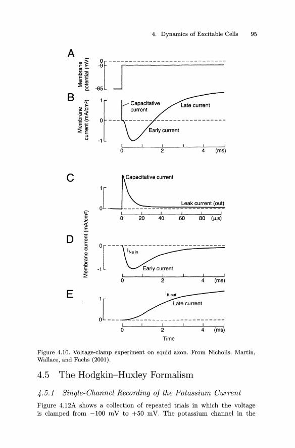
Figure 4.10B shows the clamp current during a voltage-clamp step from -65 mV to -9 mV (Figure 4.10A). This current can be broken down into the sum of four different currents: a capacitative current (Figure 4.10C), a leakage current (Figure 4.10C), a sodium current (Figure 4.10D), and a potassium current (Figure 4.10E). The potassium current turns on (activates) relatively slowly. In contrast, the sodium current activates very quickly. In addition, unlike the potassium current, the sodium current then turns off (inactivates), despite the fact that the voltage or transmembrane potential, V, is held constant.

4.4.3 Separation of the Various Ionic Currents

How do we know that the trace of Figure 4.10B is actually composed of the individual currents shown in the traces below it? This conclusion is based largely on three different classes of experiments involving ion substitution, specific blockers, and specific clamp protocols. Figure 4.11B shows the clamp current in response to a step from -65 m V to -9 m V (Figure 4.11A). Also shown is the current when all but 10% of external Na+ is replaced with an impermeant ion. The difference current (Figure 4.11C) is thus essentially the sodium current. Following addition of tetrodotoxin, a specific blocker of the sodium current, only the outward IK component remains, while following addition of tetraethylammonium, which blocks potassium channels, only the inward INa component remains.


A m> r:::: E al~

.cea E"" Q) r::::

::iEi

Of-----------------------------

~lj 8 ~

a> E r::::~ ~E .0~ E-Q) r:::: ::i!~

::::1 o

1 [ / Capacitative current

o ---

-1

4 (ms)

c

J ~ E o ~

20 80 (j.LS) 40 60

.§.

D E ~ ::::1 o Q) r:::: ~ .o E Q)

::i! o 2 4 (ms)

E

l __ Time

Figure 4.10. Voltage-clamp experiment on squid axon. From Nicholls, Martin, Wallace, and Fuchs (2001).

4.5 The Hodgkin-Huxley Formalism

4.5.1 Single-Channel Recording of the Potassium Current

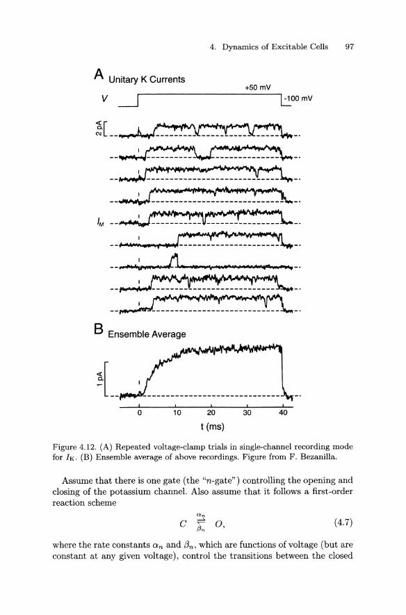
Figure 4.12A shows a collection of repeated trials in which the voltage is clamped from -100 mV to +50 mV. The potassium channel in the

96 Guevara

A

8

c

t (ms)

Figure 4.11. Effect of removal of extracellular sodium on voltage-clamp record. Adapted from Hodgkin (1958).

patch opens after a variable delay and then tends to stay open. Thus, the ensemble-averaged trace (Figure 4.12B) has a sigmoidal time course similar to the macroscopic current recorded in the axon (e.g., Figure 4.10E). It is thus clear that the macroscopic concept of the time course of activation is connected with the microscopic concept of the latency to first opening of a channel.

4.5.2 Kinetics of the Potassium Current IK The equation developed by Hodgkin and Huxley to describe the potassium current, IK, is

where !JK is the maximal conductance, and where n is a "gating" variable satisfying

Let us try to understand where this equation comes from.


A Unitary K Currents +50mV

V _j ~OOmV

B Ensemble Average

~[ __

o 10 20 30 40

t (ms)

Figure 4.12. (A) Repeated voltage-clamp trials in single-channel recording mode for lK. (B) Ensemble average of above recordings. Figure from F. Bezanilla.

Assume that there is one gate ( the "n-gate") controlling the opening and closing of the potassium channel. Also assume that it follows a first-order reaction scheme

c O, (4.7)

where the rate constants O:n and f3n, which are functions of voltage (but are constant at any given voltage), control the transitions between the closed

98 Guevara

(C) and open (O) states ofthe gate. The variable n can then be interpreted as the fraction of gates that are open, or, equivalently, as the probability that a given gate will be open. One then has

dn n 00 - n -d =an(1-n)-f3nn= ,

t Tn (4.8)

where

(4.9)

The solution of the ordinary differential equation in (4.8), when V is constant, is

(4.10)

The formula for lK would then be

(4.11)

with

dn n 00 - n dt Tn

(4.12)

where 9K is the maximal conductance. However, Figure 4.13A shows that 9K has a waveform that is not simply an exponential rise, being more sigmoidal in shape. Hodgkin and Huxley thus took n to the fourth power in equation ( 4.11), resulting in

(4.13)

Figure 4.13B shows the n 00 and Tn curves, while Figure 4.14 shows the calculated time courses of n and n4 during a voltage-clamp step.

4.5.3 Single-Channel Recording of the Sodium Current Figure 4.15A shows individual recordings from repeated clamp steps from -80 m V to -40 m V in a patch containing more than one sodium channel. Note that there is a variable latency to the first opening of a channel, which accounts for the time-dependent activation in the ensemble-averaged recording (Figure 4.15B). The inactivation seen in the ensemble-averaged recording is traceable to the fact that channels close, and eventually stay closed, in the patch-clamp recording.


A K Conductance

roi ':1~ "~

<J o

8 "' E 1:~

,,~:r, S::? (/)

.§. 20~

'tn 'tn Q)

1:~ D nco o.5 5.0 (ms)

() c: al t5 o o :::l -100 -50 o 50 "O c:

1:~ o ()o Voltage (mV) (.)

t (ms)

Figure 4.13. (A) Circles are data points for 9K calculated from experimental values of IK, V, and EK using equation (4.13). The curves are the fit using the Hodgkin-Huxley formalism. Panel A from Hodgkin (1958). (B) n= and Tn as functions of V.

4.5.4 Kinetics of the Sodium Current INa

Again, fitting of the macroscopic currents led Hodgkin and Huxley to the following equation for the sodium current, INa,

(4.14)

where m is the activation variable, and h is the inactivation variable. This implies that

) - [ ( ]3 ( ) lNa(V, t) 9Na(V, t = 9Na m V, t) h V, t = (V_ ENa) (4.15)

Figure 4.16A shows that this equation fits the 9Na data points very well. The equations directing the movement of the m-gate are very similar to

those controlling the n-gate. Again, one assumes a kinetic scheme of the form

c o, (4.16)

100 Guevara

50

- o > .s > -50

-100

1.0

0.5

0.0

o 1 2 3 4 t (ms)

Figure 4.14. Time course of n and n 4 in the Hodgkin-Huxley model.

where the rate constants O!m and f3m are functions of voltage, but are constant at any given voltage. Thus m satisfies

(4.17)

where

O!m moo = '

O!m + fJm 1

Tm = . O!m + fJm

(4.18)

The solution of equation ( 4.17) when V is constant is

m(t) = m00 - (m00 - m(O))e-tfTm. (4.19)

Similarly, one has for the h-gate

(4.20)

where the rate constants ah and fJh are functions of voltage, but are constant at any given voltage. Thus h satisfies

(4.21)


A Unitary Na Currents -40 mV

V-a~

1 -al -----N

B Ensemble Average

o 5 10 15

t (ms)

Figure 4.15. (A) Repeated voltage-clamp trials in single-channel recording mode for lNa· (B) Ensemble average of above recordings. Figure from J.B. Patlak.

where

h - O'.h 00 - O'.h + fJh'

1 Th = ·

O'.h + fJh

The solution of equation (4.21) when Vis constant is

h(t) = hoo- (hoo- h(O))e-t/Th.

(4.22)

(4.23)

102 Guevara

A Na Conductance

~:jf\;:_, 8 o 1.0

20~ 'tm

':~ (ms) -"' E o Q

CI) -50 o .s rok Voltage (mV) Q) (..") c cu 1: ~ -(..") o-::J 10.0 -o c

1:~ o (.)

5.0 'th

(ms)

10~ o o o~ o -100 -50 o 50

1 1 Voltage (mV) o 2 4

t (ms)

Figure 4.16. (A) Circles are data points for 9Na calculated from experimental values of lNa, V, and ENa using equation (4.15). The curves are the fit produced by the Hodgkin-Huxley formalism. Panel A from Hodgkin (1958). (B) m 00 , Trn,

hoo, and Th as functions of voltage.

The general formula for INa is thus

INa = .9Nam3h(V- ENa), (4.24)

with m satisfying equation (4.17) and h satisfying equation (4.21). Figure 4.16B shows m 00 , Tm, h00 , and Th, while Figure 4.17 shows the evolution of m, m 3 , h, and m 3 h during a voltage-clamp step.

4.5.5 The Hodgkin-Huxley Equations Putting together all the equations above, one obtains the Hodgkin-Huxley equations appropriate to the standard squid temperature of 6.3 degrees Celsius (Hodgkin and Huxley 1952). This is a system of four coupled nonlinear


50

- o > .s > -50

-100

1.0

o 1 2 3 4

t (ms)

Figure 4.17. Time course of m, m 3 , h, and m 3 h in the Hodgkin-Huxley model.

ordinary differential equations,

dV 1 3 4 dt = - C [(.9Nam h(V- ENa) + .9Kn (V- EK)

+ .9L(V- EL)+ fstimJ,

dm dt = am(1- m)- f3mm, (4.25)

dh dt = ah(1- h)- f3hh,

dn dt = an(1- n)- f3nn,

where

and

ENa = +55 mV, EK = -72 mV, EL= -49.387 mV, C = 1 ţ1F cm-2 .

Here fstim is the total stimulus current, which might be a periodic pulse train or a constant ( "bias") current. The voltage-dependent rate constants

104 Guevara

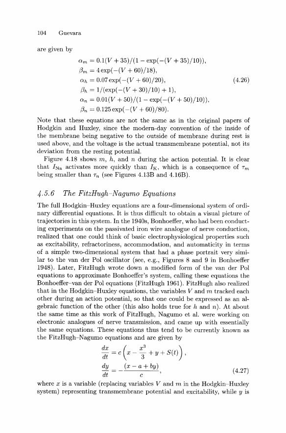
are given by

O:m = 0.1(V + 35)/(1- exp( -(V+ 35)/10)),

f3m = 4 exp( -(V+ 60)/18),

o:h = 0.07 exp( -(V+ 60)/20),

f3h = 1/(exp( -(V+ 30)/10) + 1),

O:n = O.Ol(V + 50)/(1- exp( -(V+ 50)/10)),

f3n = 0.125 exp( -(V+ 60)/80).

( 4.26)

Note that these equations are not the same as in the original papers of Hodgkin and Huxley, since the modern-day convention of the inside of the membrane being negative to the outside of membrane during rest is used above, and the voltage is the actual transmembrane potential, not its deviation from the resting potential.

Figure 4.18 shows m, h, and n during the action potential. It is clear that INa activates more quickly than IK, which is a consequence of Tm

being smaller than Tn (see Figures 4.13B and 4.16B).

4.5.6 The FitzHugh-Nagumo Equations The full Hodgkin-Huxley equations are a faur-dimensional system of ordinary differential equations. It is thus difficult to obtain a visual picture of trajectories in this system. In the 1940s, Bonhoeffer, who had been conducting experiments on the passivated iron wire analogue of nerve conduction, realized that one could think of basic electrophysiological properties such as excitability, refractoriness, accommodation, and automaticity in terms of a simple two-dimensional system that had a phase portrait very similar to the van der Pol oscillator (see, e.g., Figures 8 and 9 in Bonhoeffer 1948). Later, FitzHugh wrote down a modified form of the van der Pol equations to approximate Bonhoeffer's system, calling these equations the Bonhoeffer-van der Pol equations (FitzHugh 1961). FitzHugh also realized that in the Hodgkin-Huxley equations, the variables V and m tracked each other during an action potential, so that one could be expressed as an algebraic function of the other (this also holds true for h and n). At about the same time as this work of FitzHugh, Nagumo et al. were working on electronic analogues of nerve transmission, and carne up with essentially the same equations. These equations thus tend to be currently known as the FitzHugh-Nagumo equations and are given by

~~ = c ( x- x33 + y + S(t)) ,

dy (x-a+ by) dt c

( 4.27)

where x is a variable (replacing variables V and m in the Hodgkin-Huxley system) representing transmembrane potential and excitability, while y is


60

40

> 20

.s o -- ·---·-· --·- ---Q) Cl -20 ro -~ -40

-60

-80 o 5 10 15 20 Time (ms)

0.8

0.6

0.4

0.2 h

o o 5 10 15 20

Time (ms)

Figure 4.18. Time course of m, h, and n in the Hodgkin-Huxley model during an action potential.

a variable (replacing variables h and n in the Hodgkin-Huxley system) responsible for refractoriness and accommodation. The function S(t) is the stimulus, and a, b, and c are parameters. The computer exercises in Section 4.8 explore the properties of the FitzHugh-Nagumo system in considerable detail.

4.6 Conclusions

The Hodgkin-Huxley model has been agreat success, replicating many of the basic electrophysiological properties of the squid axon, e.g., excitability, refractoriness, and conduction speed. However, there are several discrepancies between experiment and model: For example injection of a constant bias current in the squid axon does not lead to spontaneous firing, as it does

106 Guevara

in the equations. This has led to updated versions of the Hodgkin-Huxley model being produced to account for these discrepancies (e.g., Clay 1998).

4.7 Computer Exercises: A Numerica! Study on the Hodgkin-Huxley Equations

We will use the Hodgkin-Huxley equations to explore annihilation and triggering of limit-cycle oscillations, the existence of two resting potentials, and other phenomena associated with bifurcations of fixed points and limit cycles (see Chapter 3).

The Hodgkin-Huxley model, given in equation ( 4.25), consists of a faurdimensional set of ordinary differential equations, with variables V, m, h, n. The XPP file hh.ode contains the Hodgkin-Huxley equations.* The variable V represents the transmembrane potential, which is generated by the sodium current (curna in hh.ode), the potassium current (curk), and a leak current (curleak). The variables m and h, together with V, control the sodium current. The potassium current is controlled by the variables n and V. The leak current depends only on V.

Ex. 4.7-1. Annihilation and Triggering in the Hodgkin-Huxley Equations. We shall show that one can annihilate bias-current induced firing in the Hodgkin-Huxley (Hodgkin and Huxley 1952) equations by injecting a single well-timed stimulus pulse (Guttman, Lewis, and Rinzel 1980). Once activity is so abolished, it can be restarted by injecting a strong enough stimulus pulse.

(a) Nature of the Fixed Point. We first examine the response of the system to a small perturbation, using direct numerical integration of the system equations. We will inject a small stimulus pulse to deflect the state point away from its normallocation at the fixed point. The way in which the trajectory returns to the fixed point will give us a clue as to the nature of the fixed point (i.e., node, focus, saddle, etc.). We will then calculate eigenvalues of the point to confirm our suspicions.

Start up XPP using the source file hh.ode.

The initial conditions in hh.ode have been chosen to correspond to the fixed point of the system when no stimulation is applied. This can be verified by integrating the equations numerically

*See Introduction to XPP in Appendix A.


(select Initialconds and then Go from the main XPP window). Note that the transmembrane potential (V) rests at -60 mV, which is termed the resting potential.

Let us now investigate the effect of injecting a stimulus pulse. Click on the Param button at the top of the main XPP window. In the Parameters window that pops up, the parameters tstart, duration, and amplitude control the time at which the current-pulse stimulus is turned on, the duration of the pulse, and the amplitude of the pulse, respectively (use the V, VV, /\, and /\/\ buttons to move up and down in the parameter list). When the amplitude is positive, this corresponds to a depolarizing pulse, i.e., one that tends to make V become more positive. (Be careful: This convention as to sign of stimulus current is reversed in some papers!) Conversely, a negative ampli tude corresponds to a hyperpolarizing pulse.

Change ampli tude to 10. Make an integration run by clicking on Go in this window.

You will see a nice action potential, showing that the stimulus pulse is suprathreshold.

Decrease ampli tude to 5, rerun the integration, and notice the subthreshold response of the membrane ( change the scale on the y-axis to see better if necessary, using Viewaxes from the main XPP window). The damped oscillatory response of the membrane is a clue to the type of fixed point present. Is it a node? a saddle? a focus? (see Chapter 2).

Compute the eigenvalues of the fixed point by selecting Sing Pts from the main XPP window, then Go, and clicking on YES in response to Print eigenvalues? Since the system is faurdimensional, there are four eigenvalues. In this instance, there are two real eigenvalues and one complex-conjugate pair. What is the significance of the fact that all eigenvalues have negative real part? Does this calculation of the eigenvalues confirm your guess above as to the nature of the fixed point? Do the numerica! values of the eigenvalues (printed in the main window from which XPP was originally invoked) tell you anything about the frequency of the damped subthreshold oscillation observed earlier (see Chapter 2)? Estimate the period of the damped oscillation from the eigenvalues.

108 Guevara

Let us now investigate the effect of changing a parameter in the equations.

Click on curbias in Parameters and change its value to -7. This change now corresponds to injecting a constant hyperpolarizing current of 7 J-LA/cm2 into the membrane (see Chapter 4). Run the integration and resize the plot window if necessary using Viewaxes. After a short transient at the beginning of the trace, one can see that the membrane is now resting at a more hyperpolarized potential than its original resting potential of -60 m V. How would you describe the change in the qualitative nature of the subthreshold response to the current pulse delivered at t = 20 ms? Use Sing Pts to recalculate the eigenvalues and see how this supports your answer.

Let us now see the effect of injecting a constant depolarizing current.

Change curbias to 5, and make an integration run. The membrane is now, of course, resting, depolarized to its usual value of -60 mV. What do you notice about the damped response following the delivery of the current pulse? Obtain the eigenvalues of the fixed point. Try to understand how the change in the numerica! values of the complex pair explains what you have just seen in the voltage trace.

(b) Single-Pulse Triggering. Now set curbias to 10 and remove the stimulus pulse by setting ampli tude to zero. Carry out an integration run. You should see a dramatic change in the voltage waveform. What has happened?

Recall that n is one of the four variables in the HodgkinHuxley equations. Plot out the trajectory in the (Vn)-plane: Click on Viewaxes in the main XPP window and then on 20; then enterX-axis:V, Y-axis:n, Xmin:-80, Ymin:0.3, Xmax:40, Ymax:0.8. You will see that the limit cycle ( or, more correctly, the projection of it onto the (Vn)-plane) is asymptotically approached by the trajectory. If we had chosen as our initial conditions a point exactly on the limit cycle, there would have been no such transient present. You might wish to examine the projection


of the trajectory onto other two-variable planes or view it in a three-dimensional plot (using Viewaxes and then 30, change the Z-axis variable to h, and enter O for Zmin and 1 for Zmax). Do not be disturbed by the mess that now appears! Click on Window/Zoom from the main XPP window and then on Fit. A nice three-dimensional projection of the limit-cycle appears.

Let us check to see whether anything has happened to the fixed point by our changing curbias to 10. Click on Sing pts, Go, and then YES. XPP confirms that a fixed point is stiU present, and moreover, that it is stiU stable. Therefore, if we carry out a numeri cal integrat ion run with initial conditions close enough to this fixed point, the trajectory should approach it asymptotically in time. To do this, click on Erase in the main XPP window, enter the equilibrium values of the variables V, m, h, n as displayed in the bottom of the Equilibria window into the Initial Data menu, and carry out an integration run. You will probably not notice a tiny point of light that has appeared in the 3D plot. To make this more transparent, go back and plot V vs. t, using Viewaxes and 20.

Our calculation of the eigenvalues of the fixed point and our numerica! integration runs above show that the fixed point is stable at a depolarizing bias current of 10 J.LA/cm2 • However, remember that our use of the word stable really means locally stable; i.e., initial conditions in a sufficiently small neighborhood around the fixed point will approach it. In fact, our simulations already indicate that this point cannot be globally stable, since there are initial conditions that lead to a limit cycle. One can show this by injecting a current pulse.

Change ampli tude from zero to 10, and run a simulation. The result is the startup of spontaneous activity when the stimulus pulse is injected at t = 20 ms ("single-pulse triggering"). Contrast with the earlier situation with no bias current injected.

(c) Annihilation. The converse of single-pulse triggering is annihilation. Starting on the limit cycle, it should be possible to terminate spontaneous activity by injecting a stimulus that would put the state point into the basin of attraction of the fixed point. However, one must choose a correct combination of stimulus "strength" (i.e., amplitude and duration) and timing. Search for and find a correct combination (Figure 3.20 will give you a hint as to what combination to use).

110 Guevara

(d) Supercritical Hopf Bifurcation. We have seen that injecting a depolarizing bias current of 10 MA/ cm2 allows annihilation and single-pulse triggering to be seen.

Let us see what happens as this current is increased. Put ampli tude to zero and make repeated simulat ion runs, changing curbias in steps of 20 starting at 20 and going up to 200 J1A / cm2 .

What happens to the spontaneous activity? Is there a bifurcation involved?

Pick one value of bias current in the range just investigated where there is no spontaneous activity. Find the fixed point and determine its stability using Sing pts. Will it be possible to trigger into existence spontaneous activity at this particular value of bias current? Conduct a simulation (i.e., a numerica! integration run) to back up your conclusion.

(e) Auto at Last! It is clear from the numerica! work thus far that there appears to be no limit-cycle oscillation present for bias current sufficiently small or sufficiently large, but that there is a stable limit cycle present ovcr some intermediate range of bias current ( our simulations so far would suggest somewhere between 10 and 160 J1A/cm2 ). It would be very tedious to probe this range finely by carrying out integration runs at many values of the parameter curbias, and in addition injecting pulses of various amplitudes and polarities in an attempt to trigger or annihilate activity. The thing to do here is to run Auto, man!

Open Auto by selecting File and then Auto from the main XPP window. This opens the main Auto window (It's Auto man!). Select the Parameter option in this window and replace the default choice of Pari (blockna) by curbias. In the Axes window in the main Auto menu, select hi -lo, and then, in the resulting AutoPlot window, change Xmin and Ymin to O and -80, respectively, and Xmax and Ymax to 200 and 20, respectively. These parameters control the length of the x- and y-axes of the bifurcation diagram, with the former corresponding to the bifurcation variable (bias current), and the latter to one of the four possible bifurcation variables V, m, n, h ( we ha ve chosen V). Invoke Numerica from the main Auto window, change Par Max to 200 (this parameter, together with Par Min, which is set to zero, sets the range of the bifurcation variable ( curbias) that will be investigated). Also change Nmax, which gives the maximum number of points


that Auto will compute along one bifurcation branch before stopping, to 500. Also set NPr to 500 to avoid having a lot of labeled points. Set Norm Max to 150. Leave the other parameters unchanged and return to the main Auto window. Click on the main XPP window (not the main Auto window), select ICs to bring up the Initial Data window, and click on defaul t to restore our original initial conditions (V, m, h, and n equal to -59.996, 0.052955, 0.59599, and 0.31773, respectively). Also click on default in the Parameters window. Make an integration run.

Click on Run in the main Auto window (It' s Auto man!) and then on Steady State. A branch of the bifurcation diagram appears, with the numerica! labels 1 to 4 identifying points of interest on the diagram. In this case, the point with label LAB = 1 is an endpoint (EP), since it is the starting point; the points with LAB = 2 and LAB = 3 are Hopf-bifurcation points (HB), and the point with LAB = 4 is the endpoint of this branch of the bifurcation diagram (the branch ended since Par Max was attained). The points lying on the parts of the branch between LAB = 1 and 2 and between 3 and 4 are plotted as thick lines, since they correspond to stable fixed points. The part of the curve between 2 and 3 is plotted as a thin line, indicating that the fixed point is unstable.

Click on Grab in the main Auto window. A new line of information will appear along the bottom of the main Auto window. U sing the -+ key, move sequentially through the points on the bifurcation diagram. Verify that the eigenvalues (plotted in the lower left-hand corner of the main Auto window) alllie within the unit circle for the first 4 7 points of the bifurcation diagram. At point 48 a pair of eigenvalues crosses through the unit circle, indicating that a Hopf bifurcation has occurred. A transformation has been applied to the eigenvalues here, so that eigenvalues in the left-hand complex plane (i.e., those with negative real part) now lie within the unit circle, while those with positive real part lie outside the unit circle.

Let us now follow the limit cycle created at the Hopf bifurcation point (Pt = 47, LAB = 2), which occurs at a bias current of 18.56 p,A/cm2 • Select this point with the-+ and +- keys. Then press the <Enter> key and click on Run. Note that the menu has changed. Click on Periodic. You will see a series of points

112 Guevara

(the second branch of the bifurcation diagram) gradually being computed and then displayed as circles. The open circles indicate an unstable limit cycle, while the filled circles indicate a stable limit cycle. The set of circles lying above the branch of fixed points gives the maximum of V on the periodic orbit at each value of the bias current, while the set of points below the branch of fixed points gives the minimum. The point with LAB = 5 ata bias current of 8.03 ţ.LA/cm2 is a limit point (LP) where there is a saddle-node bifurcation of periodic orbits (see Chapter 3).

Are the Hopf bifurcations sub- or supercritical (see Chapter 2)?

For the periodic branch of the bifurcation diagram, the Floquet multipliers are plotted in the lower left-hand corner of the screen. You can examine them by using Grab (use the <Tab> key to move quickly between labeled points). Note that for the stable limit cycle, all of the nontrivial multipliers lie within the unit circle, while for the unstable cycle, there is one that lies outside the unit circle. At the saddle-node bifurcation of periodic orbits, you should verify that this multiplier passes through +1 (see Chapter 3).

After all of this hard work, you may wish to keep a PostScript copy of the bifurcation diagram (using file and Postscript from the main Auto window). You can also keep a working copy of the bifurcation diagram as a diskfile for possible fu ture explorations (using File and Save diagram). Most importantly, you should sit down for a few minutes and make sure that you understand how the bifurcation diagram computed by Auto explains all of the phenomenology that you obtained from the pre-Auto (i.e., numeri cal integration) part of the exercise.

(f) Other Hodgkin-Huxley Bifurcation Parameters. There are many parameters in the Hodgkin-Huxley equations. You might try constructing bifurcation diagrams for any one of these parameters. The obvious ones to try are gna, gk, gleak, ena, ek, and eleak (see equation (4.25)).

(g) Criticat Slowing Down. When a system is close to a saddlenode bifurcation of periodic orbits, the trajectory can spend an arbitrarily long time traversing the region in a neighborhood of where the semistable limit cycle will become established at the bifurcation point. Try to find evidence of this in the system studied here.


Ex. 4.7-2. Two Stahle Resting Potentials in the Hodgkin-Huxley Equations. Under certain conditions, axons can demonstrate two stable resting potentials (see Figure 3.1 of Chapter 3). We will cornpute the bifurcation diagram of the fixed points using the modified Hodgkin-Huxley equations in the XPP file hh2sss.ode. The bifurcation parameter is now the externa! potassium concentration kout.

(a) Plotting the bifurcation diagram. This time, let us invoke Auto as directly as possible, without doing a lot of preliminary numerica! integration runs.

Make a first integration run using the source file hh2sss.ode. The transient at the beginning of the trace is due to the fact that the initial conditions correspond to a bias current of zero, and we are presently injecting a hyperpolarizing bias current of -18 ţ.LA/cm2 . Make a second integration run using as initial conditions the values at the end of the last run by clicking on Initialconds and then Last. We must do this, since we want to invoke Auto, which needs a fixed point to get going with the continuation procedure used to generate a branch of the bifurcation diagram. Start up the main Auto window. In the Parameter window enter kout for Par!. In the Axes window, enter 10, -100, 400, and 50 for Xmin, Ymin, Xmax, and Ymax, respectively. Click on Numerics to obtain the AutoNum window, and set Nmax:2000, NPr:2000, Par Min:10, Par Max:400, and Norm Max:150. Start the computation of the bifurcation diagram by clicking on Run and Steady state.

(b) Studying points of interest on the bifurcation diagram. The point with label LAB = 1 is an endpoint (EP), since it is the starting point; the points with LAB = 2 and LAB = 3 are limit points (LP), which are points such as saddle-node and saddlesaddle bifurcations, where a real eigenvalue passes through zero (see Chapter 3). The point with LAB = 4 is a Hopf-bifurcation (HB) point that we will study further later. The endpoint of this branch of the bifurcation diagram is the point with LAB = 5 (the branch ended since Par Max was attained). The points lying on the parts of the branch between LAB = 1 and 2 and between 4 and 5 are plotted as thick lines, since they correspond to stable fixed points. The parts of the curve between 2 and 3 and between 3 and 4 are plotted as thin lines, indicating that the fixed points are unstable. Note that there is a range of kout over which there are two sta-

114 Guevara

ble fixed points (between the points labeled 4 and 2).

Let us now inspect the points on the curve. Click on Grab. Verify that the eigenvalues all lie within the unit circle for the first 580 points of the bifurcation diagram. In fact, all eigenvalues are real, and so the point is a stable node.

At point 580 (LAB = 2) a single real eigenvalue crosses through the unit circle at + 1, indicating that a limit point or turning point has occurred. In this case, there is a saddle-node bifurcation of fixed points.

Between points 581 and 1086 (LAB = 2 and 3 respectively), there is a saddle point with one positive eigenvalue. The stable manifold of that point is thus of dimension three, and separates the faur-dimensional phase space into two disjoint halves.

At point 1086 (LAB = 3), a second eigenvalue crosses through the unit circle at + 1, producing a saddle point whose stable manifold, being two-dimensional, no longer divides the faurdimensional phase space into two halves. The two real positive eigenvalues collide and coalesce somewhere between points 1088 and 1089, then split into a complex-conjugate pair.

Both of the eigenvalues of this complex pair cross and enter the unit circle at point 1129 (LAB = 4). Thus, the fixed point becomes stable. A reverse Hopf bifurcation has occurred, since the eigenvalue pair is purely imaginary at this point (see Chapter 2). Press the <Esc> key to exit from the Grab function.

Keep a copy of the bifurcation diagram on file by clicking on File and Save Diagram and giving it the filename hh2sss.ode.auto.

( c) Following Periodic Orbit Emanat ing from Hopf Bifurcation Point. A Hopf bifurcation (HB) point has been found by Auto at point 1129 (LAB = 4). Let us now generate the periodic branch emanating from this HB point. Load the bifurcation diagram just computed by clicking on File and then on Load diagram in the main Auto window. The bifurcation diagram will appear in the plat window. Reduce Nmax to 200 in Numerics, select the HB point (LAB = 4) on the diagram, and generate the periodic branch by clicking on Run and then Periodic. How does the periodic branch terminate? What sort of bifurca-


tion is involved (see Chapter 3)? Plotting the period of the orbit will help you in figuring this out. Do this by clicking on Axes and then on Period. Enter 50, O, 75, and 200 for Xmin, Ymin, Xmax, and Ymax.

(d) Testing the results obtained in Auto. Return to the main XPP menu and, using direct numerica! integration, try to see whether the predictions made above by Auto (e.g., existence of two stable resting potentials) are in fact true. Compare your results with those obtained in the original study (Aihara and Matsumoto 1983) on this problem (see e.g., Figure 3.7).

Ex. 4.7-3. Reduction to a Three-Dimensional System. It is difficult to visualize what is happening in a faur-dimensional system. The best that the majority of us poor mortals can handle is a three-dimensional system. It turns out that much of the phenomenology described above will be seen by making an approximation that reduces the dimension of the equations from four to three. This involves removing the timedependence of the variable m, making it depend only on voltage.

Exit XPP and copy the file hh.ode to a new file hhminf.ode. Then edit the file hhminf.ode so that m 3 is replaced by m= 3 in the code for the equation for curna: That is, replace the line,

curna(v) = blockna*gna*mA3*h*(v-ena)

with

curna(v) = blockna*gna*minf(v)A3*h*(v-ena)

Run XPP on the source file hhminf. ode and view trajectories in 3D.

4.8 Computer Exercises: A Numerical Study on the FitzHugh-Nagumo Equations

In these computer exercises, we carry out numerica! integration of the FitzHugh-Nagumo equations, which are a two-dimensional system of ordinary differential equations.

The objectives of the first exercise below are to examine the effect of changing initial conditions on the time series of the two variables and on the phase-plane trajectories, to examine nullclines and the direction field in the phase-plane, to locate the stable fixed point graphically and numerically, to determine the eigenvalues of the fixed point, and to explore the concept of excitability. The remaining exercises explore a variety of phenomena characteristic of an excitable system, using the FitzHugh-Nagumo equations

116 Guevara

as a prototype ( e.g., refractoriness, anodal break excitation, recovery of latency and action potential duration, strength-duration curve, the response to periodic stimulation). While detailed keystroke-by-keystroke instructions are given for the first exercise, detailed instructions are not given for the rest of the exercises, which are of a more exploratory nature.

The FitzHugh-Nagumo Equations

We shall numerically integrate a simple two-dimensional system of ordinary differential equations, the FitzHugh-Nagumo equations (FitzHugh 1961). As described earlier on in this chapter, FitzHugh developed these equations as a simplification of the much more complicated-looking faur-dimensional Hodgkin-Huxley equations (Hodgkin and Huxley 1952) that describe electrica! activity in the membrane of the axon of the giant squid. They have now become the prototypical example of an excitable system, and have been used as such by physiologists, chemists, physicists, mathematicians, and other sorts studying everything from reentrant arrhythmia in the heart to controlling chaos. The FitzHugh-Nagumo equations are discussed in Section 4.5.6 in this chapter and given in equation ( 4.27). (See also Kaplan and Glass 1995, pp. 245-248, for more discussion on the FitzHugh-Nagumo equations.)

The file fhn.ode is the XPP filet containing the FitzHugh-Nagumo equations, the initial conditions, and some plotting and integrating instructions for XPP. Start up XPP using the source file fhn.ode.

Ex. 4.8-1. Numerica! Study of the FitzHugh-Nagumo equations.

(a) Time Series. Start a numerica! integration run by clicking on Ini tialconds and then Go. You will see a plot of the variable x as a function of time. Notice that x asymptotically approaches its equilibrium value of about 1.2.

Examine the transient at the start of the trace: Using Viewaxes and 2D, change the ranges of the axes by entering O for Xmin, O for Ymin, 10 for Xmax, 2.5 for Ymax. You will see that the range of t is now from O to 10 on the plot.

Now let us look at what the other variable, y, is doing. Click on Xi vs t and enter y in the box that appears at the top of the XPP window. You will note that when y is plotted as a function of t, y is monotonically approaching its steady-state value

tsee Introduction to XPP in Appendix A.


of about -0.6.

We thus know that there is a stable fixed point in the system at (x, y) ~ (1.2, -0.6). You will be able to confirm this by doing a bit of simple algebra with equation (4.27).

(b) Effect of Changing Initial Conditions. The question now arises as to whether this is the only stable fixed point present in the system. Using numerical integration, one can search for multiple fixed points by investigating what happens as the initial condition is changed in a systematic manner.

Go back and replot x as a function of t. Rescale the axes to O to 20 for t and O to 2.5 for x. Click on the ICs button at the top of the XPP window. You will see that x and y have initial conditions set to 2, as set up in the file flm.ode. Replace the the initial condition on x by -1.0. When you integrate again, you will see a second trace appear on the screen that eventually approaches the same asymptotic or steady-state value as before. Continue to modify the initial conditions until you have convinced yourself that there is only one fixed point in the system of equation (4.27).

Note: Remember that if the plot window gets too cluttered with traces, you can erase them (Erase in main XPP window).

You might also wish to verify that the variable y is also approaching the same value as before ( ~ -0.6) when the initial conditions on x and y are changed.

Reset the initial conditions to their default values. In finding the equilibria (by using Sing pts in XPP), you will see that the fixed point is stable and lies at (x*, y*) = (1.1994, -0.62426). While XPP uses numerical methods to find the roots of dx / dt = O and dyjdt =O in equation (4.27), you can very easily verify this from equation ( 4.27) with a bit of elementary algebra.

(c) Trajectory in the (xy) phase plane. We have examined the time series for x and y. Let us now look at the trajectories in the (xy) phase plane.

Change the axis settings to to X-axis: x, Y-axis: y, Xmin: -2.5, Ymin: -2 . 5, Xmax: 2. 5, Ymax: 2 . 5, and make another integratiau run. The path followed by the state-point of the system ( the

118 Guevara

trajectory) will then be displayed. The computation might proceed too quickly for you to see the direction ofmovement ofthe trajectory: However, you can figure this out, since you know the initial condition and the location of the fixed point. 'Iry several different initial conditions (we suggest the (x, y) pairs ( -1, -1), ( -1,2), (1,-1), (1,1.5)). An easy way to set initial conditions is to use the Mouse key in the Ini tialconds menu. You have probably already noticed that by changing initial conditions, the trajectory takes very different paths back to the fixed point.

To make this clear graphically, carry out simulations with the trajectory starting from an initial condition of (xo, Yo) = (1.0, -0.8) and then from (1.0, -0.9). In fact, it is instructive to plot several trajectories starting on a line of initial conditions at x = 1 (using Initialconds and then Range) with y changing in steps of 0.1 between y = -1.5 and y =O. Note that there is a critica! range of yo, in that for Yo > -0.8, the trajectory takes a very short route to the fixed point, while for y0 < -0.9, it takes a much longer route. Use Flow in the Dir. field/flow menu to explore initial conditions in a systematic way. What kind of fixed point is present (e.g., node, focus, saddle)?

(d) Nullclines and the Direction Field. The above results show that a small change in initial conditions can have a dramatic effect on the resultant evolution of the system (do not confuse this with "sensitive dependence on initial conditions").

To understand this behavior, draw the nullclines and the direction fields (do this both algebraically and using XPP). What is the sign of dx / dt in the region of the plane above the xnullcline? below the x-nullcline? How about for the y-nullcline? You can figure this out from equation (4.27), or let XPP do it for you. By examining this direction field (the collection of tangent vectors), you should be able to understand why trajectories have the shape that they do. 'Iry running a few integrations from different initial conditions set with the mouse, so that you have a few trajectories superimposed on the vector field.

(e) Excitability. The fact that small changes in initial conditions can have a large effect on the resultant trajectory is responsible for the property of excitability possessed by the FitzHugh-


Nagumo equations. Let us look at this directly.

Click on Viewaxes and then 2D. Set X-axis:t, Y-axis:x, Xmin:O.O, Ymin:-2.5, Xmax:20.0, Ymax:2.5. Set x = 1.1994 and y = -0.62426 as the new initial conditions and start an integration run. The trace is a horizontal line, since our initial conditions are now at the fixed point itself: the transient previously present has evaporated. Let us now inject a stimulus pulse. In the Param(eter) window, enter amplitude=-2.0, tstart=5.0, and duration=0.2. We are thus now set up to inject a depolarizing stimulus pulse of amplitude 2.0 and duration 0.2 time units at t = 5.0. We shall look at the trace of the auxiliary variable v, which was defined tobe equal to -x in fhn.ode. We need to look at -x, since we will now identify v with the transmembrane potential.

Using Xi vs t to plot v vs. t, you will see a "voltage waveform" very reminiscent of that recorded experimentally from an excitable cell, i.e., there is an action potential with a fast upstroke phase, followed by a phase of repolarization, and a hyperpolarizing afterpotential. Change the pulse amplitude to -1.0 and run a simulation. The response is now subthreshold. Make a phase-plane plot (with the nullclines) of the variables x and y for both the sub- and suprathreshold responses, to try to explain these two responses. Explore the range of amplitude between 0.0 and -2.0. The concept of an effective "threshold" should become clear.

Calculate the eigenvalues of the fixed point using the Sing pts menu. The eigenvalues appear in the window from which XPP was invoked. Does the nature of the eigenvalues agree with the fact that the subthreshold response resembled a damped oscillation? Predict the period of the damped oscillation from the eigenvalues and compare it with what was actually seen.

( f) Refractoriness. Modify the file fhn. ode so as to allow two successive suprathreshold stimulus pulses to be given (it might be wise to make a backup copy of the original file). Investigate how the response to the second stimulus pulse changes as the interval between the two pulses (the coupling interval) is changed. The Heaviside step-function heav(t- t0 ), which is available in XPP, is O fort < to and 1 fort> to. Is there a coupling interval below which one does not get an action potential?

120 Guevara

(g) Latency. The latency ( time from onset of stimulus pulse to upstroke of action potential) increases as the interval between two pulses is decreased. Plot latency as a function of coupling interval. Why does the latency increase with a decrease in the coupling interval?

(h) Action Potential Duration. The action potential duration ( time between depolarization and repolarization of the action potential) decreases as the coupling interval decreases. Why is this so?

(i) Strength-Duration Curve: Rheobase and Chronaxie. It is known from the earliest days of neurophysiology that a pulse of shorter duration must be of higher amplitude to produce a suprathreshold response of the membrane. Plot the threshold pulse amplitude as a function of pulse duration. Try to explain why this curve has the shape that it has. The minimum amplitude needed to provoke an action potential is termed the rheobase, while the shortest possible pulse duration that can elicit an action potential is called chronaxie.

(j) Anodal Break Response. Injecta hyperpolarizing pulse (i.e., one with a positive amplitude). Start with a pulse amplitude of 5 and increase in increments of 5. Can you explain why an action potential can be produced by a hyperpolarizing stimulus ("anodal break response")?

(k) Response to Periodic Stimulation. Investigate the various rhythms seen in response to periodic stimulation with a train of stimulus pulses delivered at different stimulation frequencies. The response of the FitzHugh-Nagumo equations to a periodic input is very complicated, and has not yet been completely characterized.

(1) Automaticity. Another basic property of many excitable tissues is automaticity: the ability to spontaneously generate action potentials. Set a = O and tmax = 50 ( click on Numerica and then Total) and run fhn.ode. What has changing the parameter a done? What is the attractor now? What has happened to the stability of the fixed point? What kind of bifurcation is involved? Changing a systematically in the range from O to 2 might assist you in answering these questions. How does the shape of the limit cycle change as a is changed?

(m) Phase-Locking. Explore the response ofthe FitzHugh-Nagumo oscillator to periodic stimulation with a periodic train of current pulses. Systematically change the frequency and amplitude of the pulse train. In another exercise (Section 5.9), phase-locking is studied in an oscillator that is simple enough to allow reduction of the dynamics to consideration of a one-dimensional map. What is the dimension of the map that would result from re-


duction of the FitzHugh-Nagumo case to a map? Can you find instances where the response of the FitzHugh-N agumo oscillator is different from that of the simpler oscillator?

Ex. 4.8-2. Two Stable Fixed Points in the FitzHugh-Nagumo Equations. In the standard version of the FitzHugh-Nagumo equations, there is only one fixed point present in the phase-space of the system. Since the x-isocline is cubic, the possibility exists for there tobe three fixed points in the FitzHugh-Nagumo equations. Try to find combinations of the parameters a, b, and c such that two stable fixed points coexist ( "bistability"). How would you have to change the FitzHugh-Nagumo equations to obtain more than two stable fixed points (i.e., multistability)?

Documents

A. Beuter et al. (eds.), Nonlinear Dynamics in Physiology